MOTION CONTROL STRATEGIES FOR NETWORKED ROBOT …robotics.mem.drexel.edu/pubs/hsieh_thesis.pdf · MOTION CONTROL STRATEGIES FOR NETWORKED ROBOT TEAMS IN ENVIRONMENTS WITH OBSTACLES

MOTION CONTROL STRATEGIES FOR NETWORKED

ROBOT TEAMS IN ENVIRONMENTS WITH

OBSTACLES

M. Ani Hsieh

A DISSERTATION

in

Mechanical Engineering and Applied Mechanics

Presented to the Faculties of the University of Pennsylvania in Partial

Fulfillment of the Requirements for the Degree of Doctor of Philosophy

2007

Vijay KumarSupervisor of Dissertation

Pedro Ponte CastanedaGraduate Group Chairperson

COPYRIGHT

M. Ani Hsieh

2007

To my mother.

iii

Acknowledgements

First and foremost, I would like to express my most sincere gratitude and admiration

to my advisor Vijay Kumar. Without his encouragement, support, and guidance,

I would never have made the decision to come to GRASP and would have never

completed this work.

My deepest thanks to the remainder of my dissertation committee, Professors

C.J. Taylor, Ali Jadbabaie, and Claire Tomlin for their comments and suggestions.

I especially want to express my gratitude to C.J. Taylor and George Pappas for

supporting me in my various endeavors throughout my time at GRASP.

Special thanks to Luiz Chaimowicz, Adam Halasz, and Savvas Loizou for the

numerous discussions, including topics that go beyond the scope of this work. Thanks

to Jonathan Fink and Nathan Michael for all their help with the indoor experiments.

Also, I would like to acknowledge everyone involved in the MARS2020 program and

the Penn Athletics Department for making Chapter 3 possible.

Additionally, I would like to thank all GRASPees whom I have had the privelege

to know and work with the last five years, especially Nora Ayanian, Dave Cappelleri,

Jim Killer, Babak Shirmohammadi, and Peng Song.

My most sincere gratitute and appreciation to my family, especially my brother

and mother, for whom all my accomplishments belong to.

Last, but always first in my heart, my deepest thanks to Anthony, for not only

iv

being my most ardent supporter, but also my most honest critic. I can’t wait to see

where this journey takes us next.

v

ABSTRACT

MOTION CONTROL STRATEGIES FOR NETWORKED ROBOT TEAMS IN

ENVIRONMENTS WITH OBSTACLES

M. Ani Hsieh

Vijay Kumar

Communication in multi-robot teams has, historically, been a means to improve con-

trol and perception. Recent advances in embedded processor technology have made

it possible to equip every robot with inexpensive off–the–shelf wireless communica-

tion capabilities. These advances have also given robots the ability to monitor and

respond to changes in the quality of their communication links. As such, progress

in multi-agent robotics and sensor networks, and particularly the convergence of the

two, will inevitably engender problems at the intersection of communication, control

and perception.

While control is necessary for successful mission execution, reliable communica-

tion is essential for coordination and cooperation in multi–robot teams. For example,

in applications such as perimeter surveillance or the cordoning off of hazardous re-

gions, robots must be capable of forming complex shapes in the plane while maintain-

ing the quality of the communication network. Thus, motion control strategies that

do not require inter–agent communication can often be beneficial since they preserve

limited bandwidth for the transmission of critical data. This is especially relevant

in teams composed of large a number of small, resource constrained agents where

bandwidth often becomes the limiting factor in agents’ abilities to communicate.

Towards this end, this thesis considers scalable motion control strategies for net-

worked robot teams that can be implemented with no inter–agent communication.

Experimental studies of strategies for maintaining end-to-end communication links

vi

for tasks like surveillance, reconnaissance, and target search and identification are

discussed in the first part of the thesis. This then motivates the work presented in

the second part: the synthesis of decentralized controllers for robot teams to form

complex patterns in two dimensions. These decentralized controllers do not require

the explicit communication of robots’ state information. Rather, agents are assumed

to be equipped with appropriate sensors, enabling them to infer relative position and

bearing information of their neighbors. The stability and convergence properties of

the controllers are presented, and the feasibility of the proposed methods is verified

via computer simulations and experimental results using two multi-robot testbeds.

vii

Contents

Acknowledgements iv

1 Introduction 1

1.1 Problem Statement . . . . . . . . . . . . . . . . . . . . . . . . . . . . 5

1.2 Maintaining Network Quality and Performance in Robot Teams . . . 6

1.3 Formation Generation and Control for Robot Swarms . . . . . . . . . 12

1.4 Organization of this work . . . . . . . . . . . . . . . . . . . . . . . . 17

2 Modeling 18

2.1 Robots . . . . . . . . . . . . . . . . . . . . . . . . . . . . . . . . . . . 18

2.1.1 Theoretical Models . . . . . . . . . . . . . . . . . . . . . . . . 18

2.1.2 Hardware . . . . . . . . . . . . . . . . . . . . . . . . . . . . . 19

2.2 Communications . . . . . . . . . . . . . . . . . . . . . . . . . . . . . 22

2.3 Controllers . . . . . . . . . . . . . . . . . . . . . . . . . . . . . . . . . 25

3 Maintaining Network Connectivity and Performance in Robot Teams 27

3.1 Multi-robot Radio Mapping . . . . . . . . . . . . . . . . . . . . . . . 29

3.1.1 Modeling . . . . . . . . . . . . . . . . . . . . . . . . . . . . . 29

3.1.2 Methodology . . . . . . . . . . . . . . . . . . . . . . . . . . . 31

3.1.3 Experimental Setup and Results . . . . . . . . . . . . . . . . . 38

viii

3.2 Reactive Controllers for Communication Link Maintenance . . . . . . 42

3.2.1 Controllers . . . . . . . . . . . . . . . . . . . . . . . . . . . . . 42

3.2.2 Link Quality Estimation . . . . . . . . . . . . . . . . . . . . . 45

3.2.3 Experimental Results . . . . . . . . . . . . . . . . . . . . . . . 47

3.2.4 Discussion . . . . . . . . . . . . . . . . . . . . . . . . . . . . . 56

3.3 Conclusion . . . . . . . . . . . . . . . . . . . . . . . . . . . . . . . . . 58

4 Scalable Motion Control Strategies for Robotic Swarms with Ob-

stacle Avoidance 61

4.1 Problem Formulation . . . . . . . . . . . . . . . . . . . . . . . . . . . 63

4.2 Methodology . . . . . . . . . . . . . . . . . . . . . . . . . . . . . . . 64

4.2.1 Assumptions . . . . . . . . . . . . . . . . . . . . . . . . . . . . 64

4.2.2 Controller Synthesis . . . . . . . . . . . . . . . . . . . . . . . 66

4.2.3 Collision Avoidance . . . . . . . . . . . . . . . . . . . . . . . . 69

4.2.4 Obstacle Avoidance . . . . . . . . . . . . . . . . . . . . . . . . 72

4.3 Safety and Stability Results . . . . . . . . . . . . . . . . . . . . . . . 74

4.4 Simulation and Experimental Results . . . . . . . . . . . . . . . . . . 81

4.4.1 Simulation Results . . . . . . . . . . . . . . . . . . . . . . . . 81

4.4.2 Experimental Results . . . . . . . . . . . . . . . . . . . . . . . 82

4.5 Extension . . . . . . . . . . . . . . . . . . . . . . . . . . . . . . . . . 85

4.5.1 Simulations . . . . . . . . . . . . . . . . . . . . . . . . . . . . 88

4.6 Conclusions and Future Work . . . . . . . . . . . . . . . . . . . . . . 88

5 Decentralized Controllers for Shape Generation with Robotic Swarms 90

5.1 Problem Formulation . . . . . . . . . . . . . . . . . . . . . . . . . . . 91

5.2 Methodology . . . . . . . . . . . . . . . . . . . . . . . . . . . . . . . 92

5.2.1 Assumptions and Definitions . . . . . . . . . . . . . . . . . . . 92

ix

5.2.2 Controller Synthesis . . . . . . . . . . . . . . . . . . . . . . . 94

5.3 Analysis . . . . . . . . . . . . . . . . . . . . . . . . . . . . . . . . . . 98

5.4 Simulations . . . . . . . . . . . . . . . . . . . . . . . . . . . . . . . . 106

5.5 Conclusions . . . . . . . . . . . . . . . . . . . . . . . . . . . . . . . . 108

6 Concluding Remarks 110

6.1 Contributions . . . . . . . . . . . . . . . . . . . . . . . . . . . . . . . 110

6.2 Future Work . . . . . . . . . . . . . . . . . . . . . . . . . . . . . . . . 113

x

List of Figures

1.1 Signal strength measurements over various distances obtained in an

environment similar to an urban park. Antennae were positioned 40

cm above the ground and the signal strength (y-axis) is normalized

to a scale of 0 - 100. . . . . . . . . . . . . . . . . . . . . . . . . . . . 9

1.2 (a) Number of transactions per interval of time between four station-

ary robots, at four distinct locations, and the Base. The number of

successful transactions between each robot and the Base drops as the

number of transmitting robots increases over time. (b) Signal strength

measurements from the robots to the Base for the same period of time. 10

2.1 The University of Pennsylvania’s MARS2020 multi-robot testbed. [14] 20

2.2 The SCARAB multi-robot testbed. . . . . . . . . . . . . . . . . . . . 21

3.1 (a) Roadmap graph G1. (b) Three different configurations that three

robots can take on the graph G1. . . . . . . . . . . . . . . . . . . . . 32

xi

3.2 (a) Radiomap graph, R, for G1 shown in Figure 3.1(a). The dashed

edges denote links for which signal strength information must be ob-

tained. (b) Three sample configurations of three robots on G1 that

can measure at least one of the edges in R. The solid vertices denote

the robots and the solid edges denote the edges that can be measured

for the given configuration. . . . . . . . . . . . . . . . . . . . . . . . . 33

3.3 (a) A sample roadmap graph G1. (b) Corresponding radiomap graph

R. . . . . . . . . . . . . . . . . . . . . . . . . . . . . . . . . . . . . . 34

3.4 (a) Graph R superimposed with G2 nodes denoted by ⊗. (b) G2 for

the G1 and R shown in Figure 3.3. . . . . . . . . . . . . . . . . . . . 35

3.5 (a) Graph R overlayed with some G3 nodes, denoted by ⊗. (b) Sub-

graph G3 for the G1 and R in Figures 3.3(a) and 3.3(b). . . . . . . . 36

3.6 (a) An overhead view of the MOUT site taken from a fixed wing UAV

at an altitude of 150 m. The area shown is approximately 90m × 120

m. (b) A manual cell decomposition of the free configuration space

for the MOUT site. . . . . . . . . . . . . . . . . . . . . . . . . . . . . 39

3.7 (a) Roadmap graph used for the site shown in Figure 3.6(a). (b)

Radiomap graph for the site shown in Figure 3.6(a). . . . . . . . . . . 41

3.8 Radio signal strength map obtained for the MOUT site. The number

on each edge is the average normalized signal strength for each position

pair. . . . . . . . . . . . . . . . . . . . . . . . . . . . . . . . . . . . . 41

3.9 (a) A satellite image of the soccer field and its surrounding. (b) De-

tailed schematic of the experimental area and its surroundings. . . . . 48

xii

3.10 (a) An overhead view of the MOUT site. The location of the Base is

denoted by © and the target locations for the team are denoted by

×. (b) The underlying communication graph for the reconnaissance

application. (c) The final positions attained by each robot and their

designated target locations, denoted by © and × respectively. . . . . 50

3.11 Robots’ distances to their respective goals over time. The data is

obtained using each robot’s raw GPS data with approximately 2–3

meters in accuracy. . . . . . . . . . . . . . . . . . . . . . . . . . . . . 50

3.12 Schematic of experimental setup and underlying communication graph

for the results shown in Figure 3.13. On the left, the dashed line de-

notes the communication link monitored by the robot. In this experi-

ment, Robot 2 was used to cause a network disturbance by transmit-

ting to the Base. . . . . . . . . . . . . . . . . . . . . . . . . . . . . . 53

3.13 Top: Number of transactions received by the Base from Robot 1 and

Robot 2 over time. Robot 2 began its transmission at around t = 130s.

Center Top: 1 denotes Robot 1 achieved the target transaction rate

and 0 otherwise. Center Bottom: Actual speed achieved by Robot

1. Positive speed denotes the robot is moving towards the goal and

negative speed denotes the robot is moving towards the Base. Bottom:

Robot 1’s distance from the goal. . . . . . . . . . . . . . . . . . . . . 54

3.14 Schematic of experimental setup and underlying communication graph

for the results shown in Figure 3.15 and 3.16. Similarly, the dashed

lines in the figure on the left denote communication links monitored

by each robot. . . . . . . . . . . . . . . . . . . . . . . . . . . . . . . . 55

xiii

3.15 Top: Signal strength measured by Robot 1 to the Base. The solid

black line denotes the minimum acceptable level. Center: Com-

manded speed based on the signal strength measurements. Positive

speed denotes Robot 1 is moving towards the goal and negative speed

denotes it is moving towards the Base. Bottom: Estimated speed

achieved by Robot 1 based on the commanded speed. Data for Robots

2, 3 and 4 are similar and thus not shown. . . . . . . . . . . . . . . . 56

3.16 (a) Top: 1 denotes the target transaction rate was achieved and 0

otherwise. Bottom: Commanded speed based on whether the target

transaction rate was achieved. Positive speed denotes Robot 1 is mov-

ing towards the goal and negative speed denotes it is moving towards

the Base. (b) Top: Actual speed achieved by Robot 1 based on the

commanded speed. Bottom: Robot 1’s distance from the goal. Data

for Robots 2, 3 and 4 are similar and thus not shown. . . . . . . . . . 57

4.1 (a) A star shape whose boundary is given by r−(a0+b0 sin(c0θ+d0)) =

0 with a0 = 20, b0 = 1, c0 = 5, and d0 = π/2. (b) The shape

navigation function for the boundary given in (a). . . . . . . . . . . . 67

4.2 Vector fields for the star shaped boundary given by r−(a0+b0 sin(c0θ+

d0)) = 0 with a0 = 20, b0 = 1, c0 = 5, and d0 = π/2. (a) Vector field

given by −∇ϕ. (b) Vector field given by −∇ × ψ. (c) Vector field

given by equation (4.3) with f(Ni) = 1 and g(Ti) = 1. . . . . . . . . . 68

4.3 Graph of σ−(w) with t1 = t2 = 2. . . . . . . . . . . . . . . . . . . . . 71

xiv

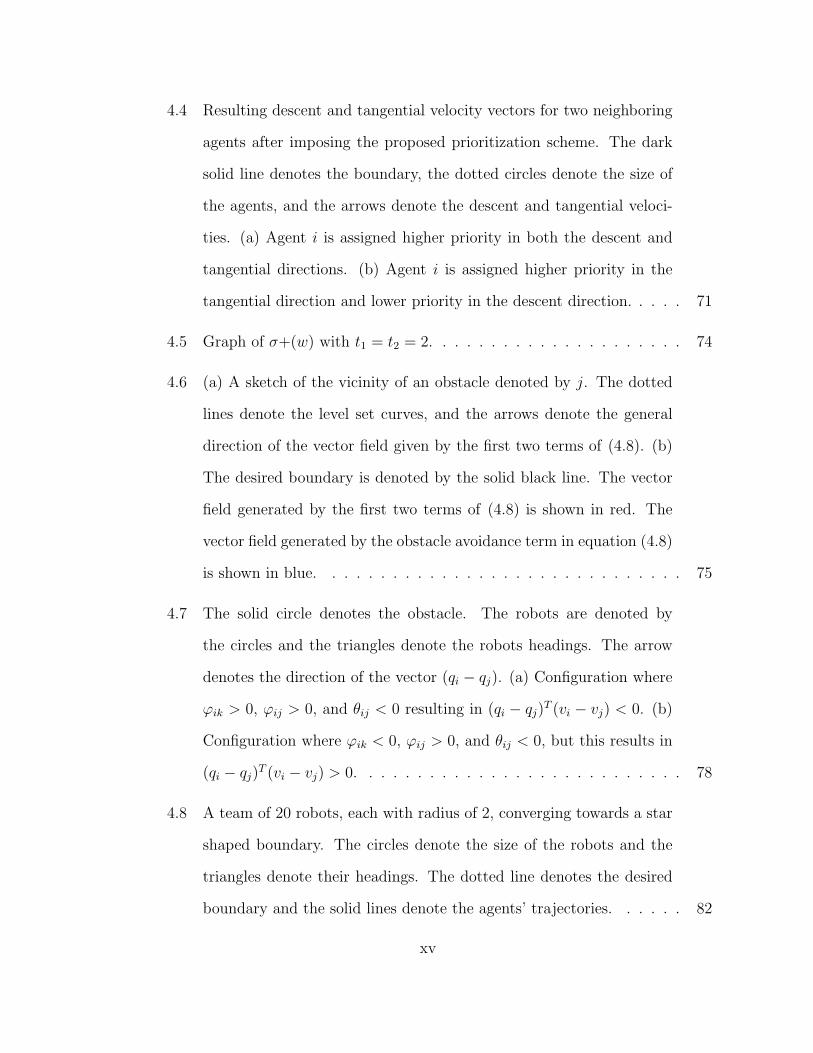
4.4 Resulting descent and tangential velocity vectors for two neighboring

agents after imposing the proposed prioritization scheme. The dark

solid line denotes the boundary, the dotted circles denote the size of

the agents, and the arrows denote the descent and tangential veloci-

ties. (a) Agent i is assigned higher priority in both the descent and

tangential directions. (b) Agent i is assigned higher priority in the

tangential direction and lower priority in the descent direction. . . . . 71

4.5 Graph of σ+(w) with t1 = t2 = 2. . . . . . . . . . . . . . . . . . . . . 74

4.6 (a) A sketch of the vicinity of an obstacle denoted by j. The dotted

lines denote the level set curves, and the arrows denote the general

direction of the vector field given by the first two terms of (4.8). (b)

The desired boundary is denoted by the solid black line. The vector

field generated by the first two terms of (4.8) is shown in red. The

vector field generated by the obstacle avoidance term in equation (4.8)

is shown in blue. . . . . . . . . . . . . . . . . . . . . . . . . . . . . . 75

4.7 The solid circle denotes the obstacle. The robots are denoted by

the circles and the triangles denote the robots headings. The arrow

denotes the direction of the vector (qi − qj). (a) Configuration where

ϕik > 0, ϕij > 0, and θij < 0 resulting in (qi − qj)T (vi − vj) < 0. (b)

Configuration where ϕik < 0, ϕij > 0, and θij < 0, but this results in

(qi − qj)T (vi − vj) > 0. . . . . . . . . . . . . . . . . . . . . . . . . . . 78

4.8 A team of 20 robots, each with radius of 2, converging towards a star

shaped boundary. The circles denote the size of the robots and the

triangles denote their headings. The dotted line denotes the desired

boundary and the solid lines denote the agents’ trajectories. . . . . . 82

xv

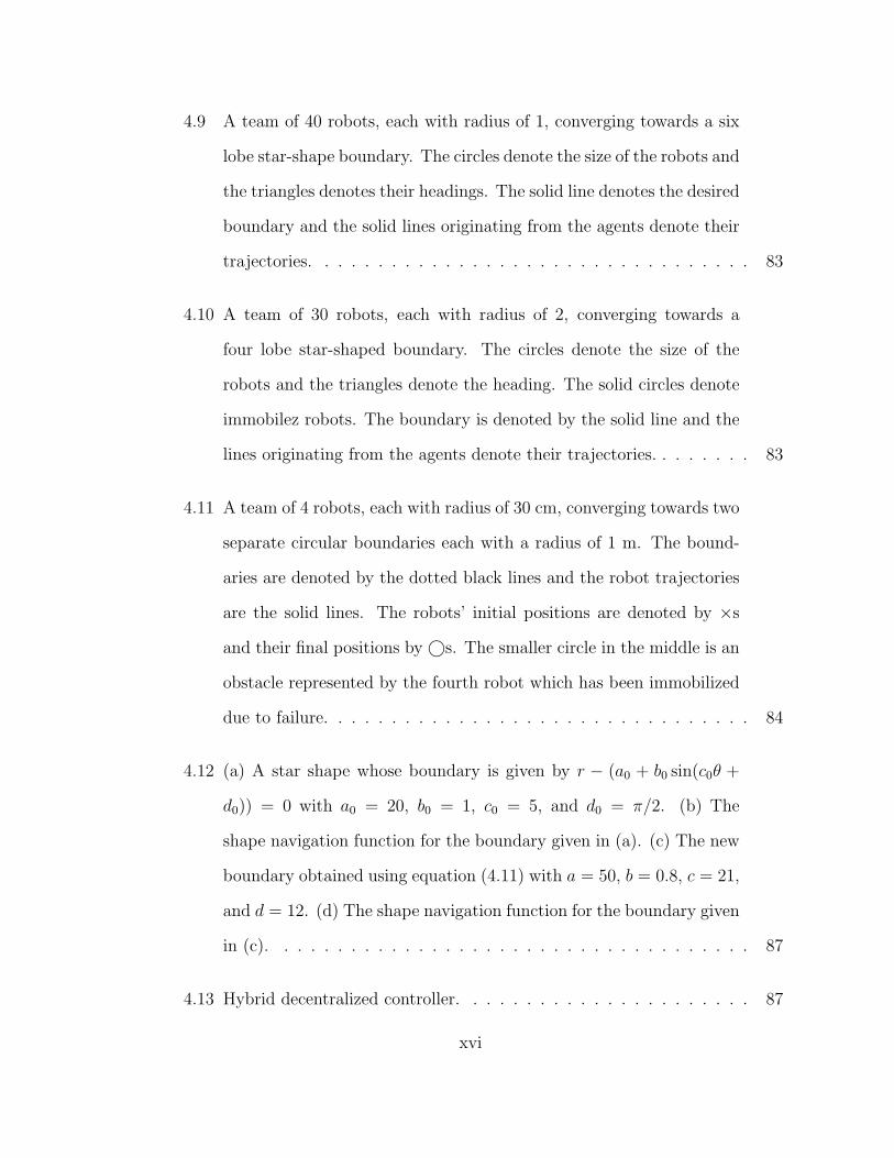
4.9 A team of 40 robots, each with radius of 1, converging towards a six

lobe star-shape boundary. The circles denote the size of the robots and

the triangles denotes their headings. The solid line denotes the desired

boundary and the solid lines originating from the agents denote their

trajectories. . . . . . . . . . . . . . . . . . . . . . . . . . . . . . . . . 83

4.10 A team of 30 robots, each with radius of 2, converging towards a

four lobe star-shaped boundary. The circles denote the size of the

robots and the triangles denote the heading. The solid circles denote

immobilez robots. The boundary is denoted by the solid line and the

lines originating from the agents denote their trajectories. . . . . . . . 83

4.11 A team of 4 robots, each with radius of 30 cm, converging towards two

separate circular boundaries each with a radius of 1 m. The bound-

aries are denoted by the dotted black lines and the robot trajectories

are the solid lines. The robots’ initial positions are denoted by ×s

and their final positions by©s. The smaller circle in the middle is an

obstacle represented by the fourth robot which has been immobilized

due to failure. . . . . . . . . . . . . . . . . . . . . . . . . . . . . . . . 84

4.12 (a) A star shape whose boundary is given by r − (a0 + b0 sin(c0θ +

d0)) = 0 with a0 = 20, b0 = 1, c0 = 5, and d0 = π/2. (b) The

shape navigation function for the boundary given in (a). (c) The new

boundary obtained using equation (4.11) with a = 50, b = 0.8, c = 21,

and d = 12. (d) The shape navigation function for the boundary given

in (c). . . . . . . . . . . . . . . . . . . . . . . . . . . . . . . . . . . . 87

4.13 Hybrid decentralized controller. . . . . . . . . . . . . . . . . . . . . . 87

xvi

4.14 A team of 13 robots each with radius of 2, converging towards a star-

shaped boundary. Eventually, a robot, denoted by the solid circle, is

immobilized in close proximity to the boundary. The circles denote the

size of the robots and the triangles denotes the heading. The boundary

is denoted by the solid black line, and the solid lines originating from

the agents denote the agents’ trajectories. . . . . . . . . . . . . . . . 89

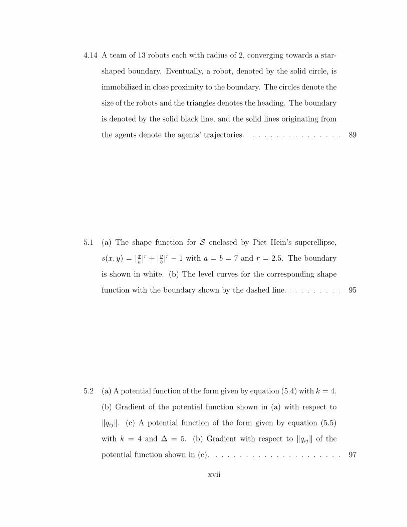
5.1 (a) The shape function for S enclosed by Piet Hein’s superellipse,

s(x, y) = |xa|r + |y

b|r − 1 with a = b = 7 and r = 2.5. The boundary

is shown in white. (b) The level curves for the corresponding shape

function with the boundary shown by the dashed line. . . . . . . . . . 95

5.2 (a) A potential function of the form given by equation (5.4) with k = 4.

(b) Gradient of the potential function shown in (a) with respect to

‖qij‖. (c) A potential function of the form given by equation (5.5)

with k = 4 and ∆ = 5. (b) Gradient with respect to ‖qij‖ of the

potential function shown in (c). . . . . . . . . . . . . . . . . . . . . . 97

xvii

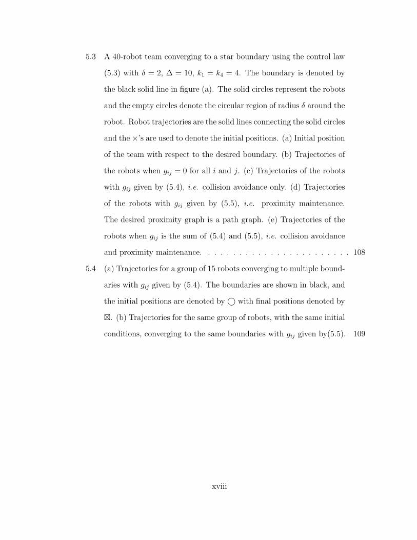
5.3 A 40-robot team converging to a star boundary using the control law

(5.3) with δ = 2, ∆ = 10, k1 = k4 = 4. The boundary is denoted by

the black solid line in figure (a). The solid circles represent the robots

and the empty circles denote the circular region of radius δ around the

robot. Robot trajectories are the solid lines connecting the solid circles

and the ×’s are used to denote the initial positions. (a) Initial position

of the team with respect to the desired boundary. (b) Trajectories of

the robots when gij = 0 for all i and j. (c) Trajectories of the robots

with gij given by (5.4), i.e. collision avoidance only. (d) Trajectories

of the robots with gij given by (5.5), i.e. proximity maintenance.

The desired proximity graph is a path graph. (e) Trajectories of the

robots when gij is the sum of (5.4) and (5.5), i.e. collision avoidance

and proximity maintenance. . . . . . . . . . . . . . . . . . . . . . . . 108

5.4 (a) Trajectories for a group of 15 robots converging to multiple bound-

aries with gij given by (5.4). The boundaries are shown in black, and

the initial positions are denoted by© with final positions denoted by

. (b) Trajectories for the same group of robots, with the same initial

conditions, converging to the same boundaries with gij given by(5.5). 109

xviii

Chapter 1

Introduction

Nikola Tesla first proposed and demonstrated the principles of wireless communica-

tion to the National Electric and Light Association in 1893. He followed this with

the exhibition of two radio remote–controlled boats in the Electrical Exhibition at

New City’s Old Madison Square Garden in 1898. Despite Tesla’s faith in military

applications of wireless communication, the technology remained a novelty until the

advent of the television remote controller in the 1950s. Nevertheless, the foundation

for all present day remote operated vehicles such as the Mars Rovers and Predator

drones, and all multi–robot systems, was laid by Tesla almost half a century before

Isaac Assimov introduced the word ”robotics” to the modern day vernacular [94–97].

In addition to the television remote control, the 1950s also saw the births of

modern robotics, and of the first multi–robot system, built by a biologist named

W. Grey Walter. Walter’s system consisted of two electronic, completely analog,

autonomous robots with rudimentary navigation and obstacle avoidance capabilities.

Much like Tesla’s original conception of radio remote-controlled vehicles, these and

other robots of the 1960s remained novelties until the late 1970s with the invention

of the robotic manipulator. This event transformed the manufacturing industry and

1

heralded the era of the automated assembly line.

Today, with the ever decreasing price to performance ratio of embedded proces-

sors and sensors, and increasingly ubiquitous wireless technology, automation has

permeated every day life with robots poised to do the same. In 2004, industrial

robots alone accounted for a $4 billion dollar market, with the personal service,

entertainment, and domestic robot sector estimated at over $3.5 billion [9]. These

advances that have made individual robots smaller, more capable, and less expensive

have also enabled the development and deployment of teams of robotic agents.

While multi-robot systems may seem like a recent paradigm shift brought on

by the latest technological advances, research in the field began almost at the con-

ception of the robotic manipulator. In the early 1980s, the focus was primarily on

the control and coordination of multiple robotic arms for cooperative grasping and

handling of large objects [8]. Then in 1986, California established the Partners for

Advanced Transit and Highways (PATH) program in an attempt to find novel ways

to address the traffic congestion problem. The program generated much interest in

the areas of automated highway systems and helped advance research in areas like

autonomous vehicle platooning and formation maintenance [91]. However, the vi-

sion, and the motivation, for multi-robot systems were not clearly set forth until the

1988 publication of “Gnat Robots: A low-intelligence, low-cost approach” by Anita

Flynn where she claimed:

With low cost and small size, we can begin to envision massive paral-lelism, using millions of small simple robots to perform tasks that mightotherwise be done with one large, expensive, complex robot. In addi-tion, we also begin to view our robots as disposable. They can be cheapenough that they are thrown away when they have finished their missionor are broken, and we do not have to worry about retrieving them fromhazardous or hard to reach places. [34]

2

Today, multi-robot systems have been deployed for tasks like environmental monitor-

ing [3,48,83], surveillance of indoor environments [78] and support for first responders

in search and rescue operations [52]. While there are many successful embodiments

of multi-robot systems with numerous applications, they are still mostly found in

the manufacturing industry where robots operate in structured environments exe-

cuting fixed tasks with no variations in operating conditions. On the other hand,

urban and unstructured envrionments provide unique challenges for the deployment

of multi-robot teams. In these environments, buildings and large obstacles pose 3-D

constraints on visibility, communication network performance is difficult to predict,

and GPS measurements can be unreliable or even unavailable.

Consider the vision of the MARS2020 program funded by the Defense Advanced

Research Projects Agency (DARPA). The collaborative effort between the General

Robotics, Automation, Sensing & Perception (GRASP) Laboratory at the Univer-

sity of Pennsylvania, Georgia Tech Mobile Robot Laboratory and the University of

Southern California’s (USC) Robotic Embedded Systems Laboratory required the

deployment of a heterogeneous team of aerial and ground autonomous robots with

the vision of providing a framework that would enable deployment by a single hu-

man operator. Once deployed, the team of autonomous air and ground robots would

cooperatively execute tasks such as surveillance, reconnaissance, and target search

and localization within an urban environment while providing high-level situational

awareness for the remote human operator. The framework would enable autonomous

robots to synthesize the desirable features and capabilities of both deliberative and

reactive control while incorporating a capability for learning, and include a software

composition methodology that incorporates both pre-composed coding and learning-

derived or automated coding software to increase the ability of autonomous robots

to function in unpredictable environments. A team of heterogeneous robots with

3

such capabilities has the potential to efficiently and accurately characterize the envi-

ronment and to exceed the performance of human agents. As such, the objectives of

the program were the development and demonstration of an architecture along with

algorithms and software tools that:

• are independent of team composition;

• are independent of team size, i.e. number of robots;

• are able to execute a wide range of tasks;

• allow a single operator to command and control the team;

• allow for interactive interrogation and/or reassignment of any robot by the

operator at the task or team level.

From our MARS2020 experience, such goals of coordinating multiple autonomous

units, and making them cooperate inherently create problems at the intersection of

communication, control and perception. While control is necessary for sucessful mis-

sion execution, reliable communication is essential for coordination and cooperation

in multi-robot teams, particularly at the level required by the MARS2020 vision.

The prevalence of wireless technology has made it possible to inexpensively outfit

every agent with some off–the–shelf wireless networking solution, however, the level

of coordination required by the MARS2020 program would mean robots must also

be able to perceive changes in their abilities to communicate, anticipate information

needs of other network users, and reposition/self-organize themselves to best ac-

quire and deliver the relevant information, and as such provide seamless situational

awareness within various types of environments.

4

1.1 Problem Statement

With this in mind, the first part of the thesis is concerned with strategies for main-

taining end-to-end communication links in a multi-robot team. Specifically, the cou-

pling of high-level planning with low-level reactive controllers for communication link

maintenance is presented along with experimental results considering the differences

between monitoring inter-agent signal strengths versus data throughput. The second

part of this thesis is concerned with the synthesis of provably correct scalable motion

control strategies for circular robots of finite size. Specifically, we are interested in

strategies that will enable a team of robots to form complex shapes in the plane

while avoiding colllisions using little to no inter-robot communication. This is rele-

vant because bandwidth is often the limiting factor in agents’ abilities to transmit

critical data in large teams. As such, robots must not only have the ability to form

complex shapes, they must do so with as little communication overhead as possible

to ensure reliable communication of crucial data with other team members or to

a remote base station. Lastly, we extend our proposed motion coordination strat-

egy to second order dynamic systems and incorporate some of the link maintenance

strategies presented in the first part to synthesize decentralized feedback controllers

for pattern generation while maintaining team connectivity.

In summary, the contributions of this thesis are two-fold: 1) experimentally ver-

ified strategies for maintaining point-to-point communication links in multi-robot

teams and 2) provably correct methods for scalable motion synthesis for large teams

of robots with obstacle avoidance. The motivations for these areas and a review of

the relevant literature are provided in the following sections.

5

1.2 Maintaining Network Quality and Performance

in Robot Teams

In recent years, the communication network has evolved from being just a medium

of information transmission to an actual sensor, where properties like connectivity

and signal strength are used to maintain the quality of the medium [7, 37, 73, 85].

Agents can use communication links to infer their individual locations with respect to

those of their neighbors and other landmarks. Simultaneously, agents may also con-

trol their position and orientation relative to other agents to sustain communication

links. We are interested in developing robotic teams that can operate autonomously

in urban and/or hazardous areas and perform tasks such as surveillance, target

search and identification, and reconnaissance all while maintaining team connectiv-

ity. These tasks are relevant in applications such as urban search and rescue, and

environmental monitoring for homeland security, to name a few. We note that while

the maintenance of network connectivity is required for useful situational aware-

ness and system responsiveness, often the very environments we wish to operate in

make this extremely challenging, especially when the mobile robots consist of small,

lightweight ground vehicles that operate very close to the ground.

The growing interest in the convergence of the areas of multi-agent robotics and

sensor networks has spurred interest in the development of networks of sensors and

robots that can perceive their environment and respond to it. Much of the research in

the mobile wireless network community has been devoted to the development of novel

algorithms to handle packet routing [1, 99], resource allocation [31], and bandwidth

management [61] for mobile nodes. However, control of mobile robot teams provides

us with the capability to shape the team’s communication needs based on continuous

evaluation of the demands on the network [7].

6

One of the earliest works studying the effects of communication on multi-agent

systems is the work by Dudek et al. where the effects of two-way, one-way, and

completely implicit communication and sensing in a leader follower task was consid-

ered [30]. This, along with other works like the one by Winfield [98], and Arkin and

Diaz [5], often assumed constant communication ranges and/or relied on line-of-sight

maintenance for communication. Other examples include the works by Pereira [67]

and Sweeney et al. [85], where decentralized controllers for concurrently moving

toward goal destinations while maintaining relative distance and line-of-sight con-

straints were respectively presented; and the discussion of the fomration of com-

munication relays between any pair of robots using line-of-sight was discussed by

Anderson et al. [4]. Although coordination strategies that rely on line-of-sight main-

tenance may significantly improve each agent’s ability to communicate, it has been

shown through simulation by Thibodeau et al. [90], that line-of-sight maintenance

strategies are often not necessary and may potentially be too restrictive. This work

showed through simulations that coordination strategies based on line-of-sight main-

tenance for cooperative mapping are overall less efficient than strategies based on

inter-agent wireless signal strengths.

Recent works that consider coordination strategies based on inter-agent signal

strength include one by Wagner and Arkin where the combination of planning and

reactive behaviors for was used for communication link maintenance in a multi-

robot team conducting reconnaissance [93]. In this work, robots are tasked to go to

different goal positions while maintaining communication links with the base station

and/or a communication relay robot. In the event the robots sense a drop in the

quality of their communication link(s), a contingency plan, i.e. a plan used to

re-establish network connectivity, is triggered. In this case, the contingency plan

re-tasked the robots to go to a location within the workspace selected a priori.

7

Simulation results were presented for teams of two to four robots. In general, goal

positions are determined and planned based on all available information including

radio transmission properties. However, most reasonably ambitious missions run

the risk of encountering situations that were not reflected in planning. In the case

of radio signal propagation in urban environments, one could rely on simulation

validation of a plan, however this would require one to be extremely conservative

in mission planning due to the difficulty in accurately predicting radio transmission

characteristics.

Navigation based on perceived wireless signal strength between robots for explo-

ration was presented by Sweeney et al. [86]. Here a null-space projection approach

was used to navigate each robot towards its goal while maintaining point-to-point

communication links. This work included simulation results for a team of four planar

robots. Powers and Arkin [73] proposed a strategy where individual agents made

control decisions based on their actual and predicted signal strength measurements

while moving towards a goal. Simulation results for teams of one to four robots

with and without the controller were presented. Although coordination strategies

based on inter-agent signal strength can significantly improve overall performance,

they do not account for the effects of team size on overall network performance. As

team size increases, bandwidth becomes a limiting factor since an acceptable level

of signal strength no longer guarantees a robot’s ability to transmit critical data.

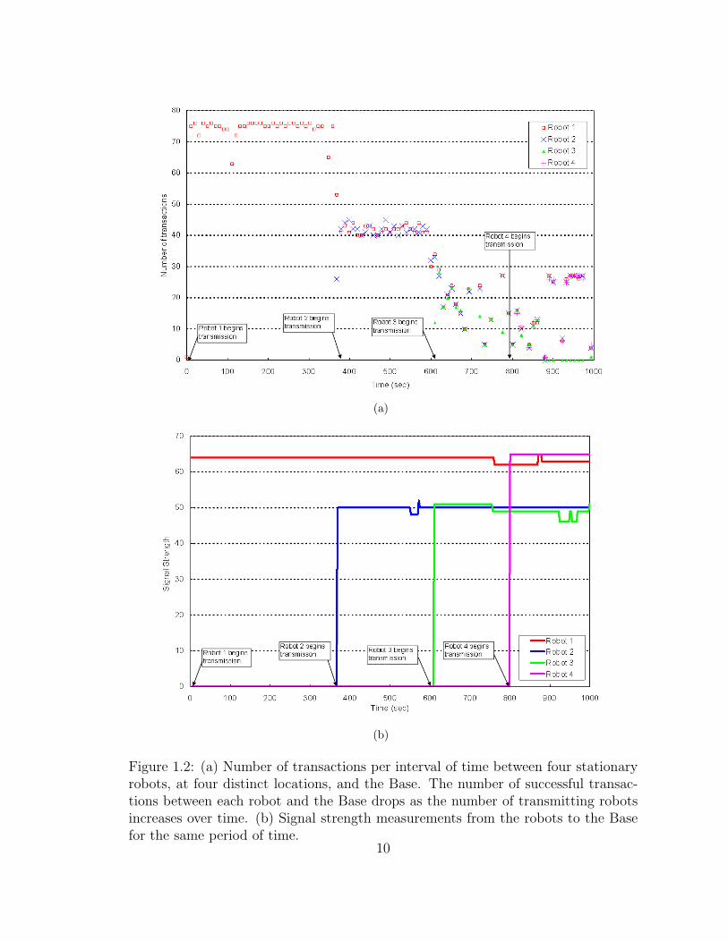
Figure 1.2(a) shows the number of transactions1 per interval of time between

four different robots, positioned at four distinct fixed locations, and a fifth station-

ary robot which we call the Base. Initially, one robot is transmitting at the maximum

data rate supported by the network. As the second, third and fourth robots succes-

sively begin their transmissions to the Base, we see not only a drop in the bandwidth

1This metric is defined more precisely later in Section 3.2.2.

8

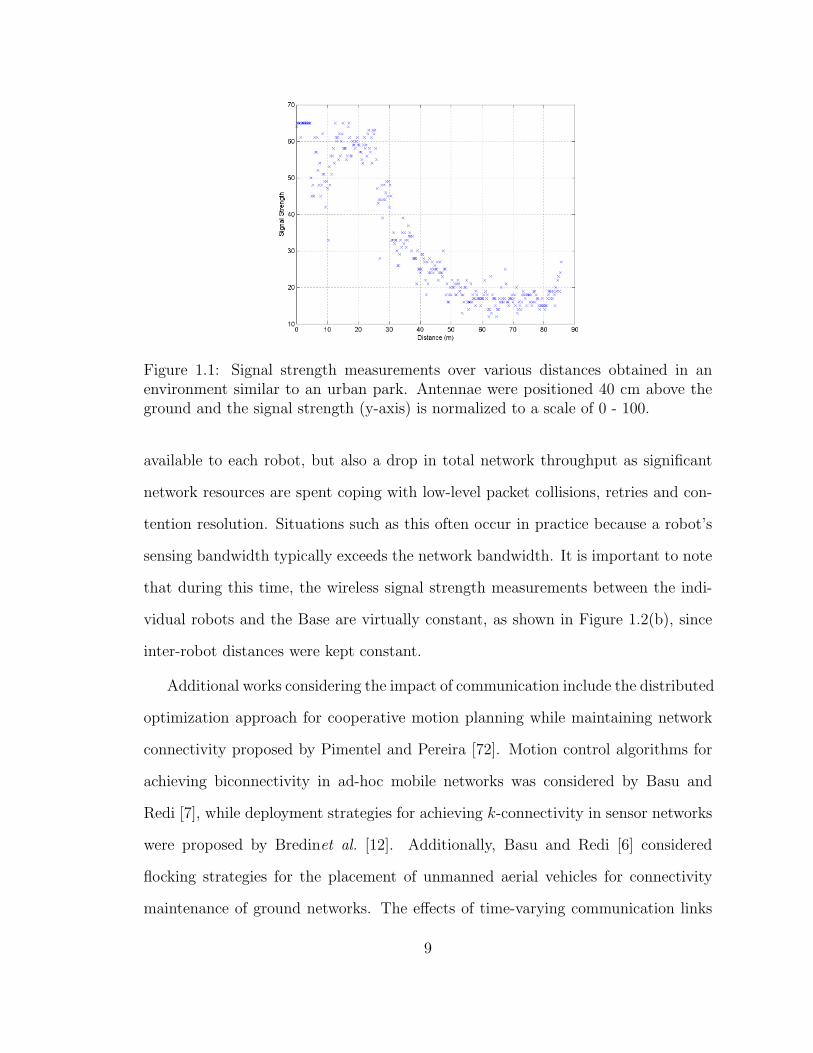
Figure 1.1: Signal strength measurements over various distances obtained in anenvironment similar to an urban park. Antennae were positioned 40 cm above theground and the signal strength (y-axis) is normalized to a scale of 0 - 100.

available to each robot, but also a drop in total network throughput as significant

network resources are spent coping with low-level packet collisions, retries and con-

tention resolution. Situations such as this often occur in practice because a robot’s

sensing bandwidth typically exceeds the network bandwidth. It is important to note

that during this time, the wireless signal strength measurements between the indi-

vidual robots and the Base are virtually constant, as shown in Figure 1.2(b), since

inter-robot distances were kept constant.

Additional works considering the impact of communication include the distributed

optimization approach for cooperative motion planning while maintaining network

connectivity proposed by Pimentel and Pereira [72]. Motion control algorithms for

achieving biconnectivity in ad-hoc mobile networks was considered by Basu and

Redi [7], while deployment strategies for achieving k-connectivity in sensor networks

were proposed by Bredinet al. [12]. Additionally, Basu and Redi [6] considered

flocking strategies for the placement of unmanned aerial vehicles for connectivity

maintenance of ground networks. The effects of time-varying communication links

9

(a)

(b)

Figure 1.2: (a) Number of transactions per interval of time between four stationaryrobots, at four distinct locations, and the Base. The number of successful transac-tions between each robot and the Base drops as the number of transmitting robotsincreases over time. (b) Signal strength measurements from the robots to the Basefor the same period of time.

10

on control performance of a mobile sensor node over a wireless network and in dis-

tributed sensing and target tracking was analyzed by Mostofi and Murray [58, 59].

The use of wireless communication for localization was presented by Howard [37]

and for localization and navigation was presented by Corke et al. [20]. Deployment

strategies for a mobile sensor network to control sensor node density were considered

by Zhang and Sukhatme [100]. An exploration methodology for a multi-robot team

to map the radio propagation characteristics of an urban environment was proposed

by Hsieh et al. [41]. Lindhe et al. studied the effects of multi-path fading and

developed a strategy of exploiting the fading for robot communications in [54].

In general, it is difficult to predict radio transmission properties a priori due to

their sensitivity to a variety of factors including transmission power, terrain charac-

teristics, and interference from other sources. Most existing propagation models as-

sume transmission distances of approximately 100–200 meters with antennae placed

high above the ground [62], and are not applicable to small, lightweight mobile nodes

operating with low transmission power. This is because, at these small scales, the

signal propagation mechanism is often dominated by the effects of reflection and

scattering making modeling especially challenging in unexplored and unstructured

environments.

In the first part of this work, we present techniques for ground vehicles connected

via a wireless network to collaboratively perform surveillance tasks while providing

situational awareness to an operator. We first show how nominal models of an

urban environment can be used to generate strategies for exploration and present

the construction of a radio signal strength map that can be used to plan multi-

robot tasks and also serve as useful perceptual information. Additionally, we present

reactive controllers for communication link maintenance. These controllers can be

used in conjunction with information gleaned from our radio signal strength maps

11

to enable our robots to adapt to changes in actual signal strength or estimated

available bandwidth. We describe techniques to aid in planning robotic missions

subject to connectivity constraints, and a reactive technology layer that maintains

those constraints that may be composed with other controllers.

1.3 Formation Generation and Control for Robot

Swarms

The advances in embedded processor and sensor technology that have made individ-

ual robots smaller, more capable, and less expensive have also enabled the develop-

ment and deployment of teams of robotic agents, where capabilities are expressed

by populations rather than super-capable individuals. As team sizes increase, it is

often difficult, if not impossible, to efficiently manage or control the team through

centralized algorithms or tele–operation. Accordingly, it makes sense to develop

strategies where robots can be programmed with simple but identical behaviors that

can be realized with limited on–board computational, communication and sensing

resources.

In nature, the emergence of complex group level behaviors from simple agent

level behaviors is often seen in the group dynamics of bee [13] and ant [74] colonies,

bird flocks [24], and fish schools [66]. These systems generally consist of large num-

bers of organisms that individually lack either the communication or computational

capabilities required for centralized control. As such when considering the deploy-

ment of large robot teams, it makes sense to consider such “swarming paradigms”

where agents have the capability to operate asynchronously and can determine their

trajectories based on local sensing and/or communication.

12

One of the earliest works to take inspiration from biological swarms for motion

generation was presented by Reynolds in 1987 [76] where he proposed a method

for generating visually satisfying computer animations of bird flocks, often referred

as boids. Almost a decade later, Vicsek et al. showed through simulations that

a team of autonomous agents moving in the plane with same speed but different

headings converge to the same heading using nearest neighbor update rules [92]. The

theoretical explanation for this observed phenomena was provided by Jadbabaie et al.

[46] and Tanner et al. [87] extended these results to provide a detailed analysis of the

stability and robustness of such flocking behaviors. Olfati-Saber then extended some

of the results in these works to address the design and analysis of distributed flocking

algorithms for robot teams in free–space and in environments with obstacles [64] .

These works show that teams of autonomous agents can stably achieve concensus

through local interactions alone, i.e. without centralized coordination, and have

attracted much attention in the multi-robot community.

Previous works in group coordination using decentralized controllers to synthe-

size geometric patterns include the works by Albayrak et al. [2] and Suzuki et al. [84].

While Albayrak et al. only considered line and circle formations [2] , more general

geometric patterns were considered by Suzuki et al. [84]. These aproaches, how-

ever, assume that each robot has full knowledge of the positions of all the other

robots. Another approach to team formation is via a leader-follower formulation.

One of the earliest synthesis of decentralized leader-follower controllers for robot

formations was proposed by Desai et al. [25]. Although the controllers were decen-

tralized, the methodology requires the assignment of different controllers and set

points to different robots, making scaling to large groups difficult. Another decen-

tralized leader-follower approach to formation control was presented by Fierro et

al. [32]. Here, the authors established the asymptotic stability of the leader-follower

13

formation control for a group of nonholonomic robots in SE(2). Leader-follower

controllers, in general, require the labeling of robots; Ogren et al. relaxed this as-

sumption in the development of coordination strategies for a group of unidentified,

holonomic robots [63].

Navigation function based approaches for multi-robot coordination include the

works by Tanner et al. [88], Loizou et al. [55], and by Dimarogonas et al. [26]. While

these works concern the motion coordination of non-point agents, they assume global

sensing capabilities. This requirement was relaxed by Dimarogonas in [27] and ex-

tended to dynamic systems in [28], however, the resulting methodologies still require

knowledge of team size which makes the addition and deletion of agents difficult.

Other similar approaches for multi-robot manipulation are presented by Song and

Kumar [81] and Pereira and Kumar [68] respectively. Chaimowicz et al. extended

these approaches to arbitrary shapes and established convergence to patterns that

approximate the desired shape [17]. With the exception of [55], the controllers

in [17, 68, 81] enabled the team to converge to the boundary of some desired two-

dimensional shape in the plane. The stability and convergence properties of these

potential field based controllers with inter-agent constraints for a class of boundaries

were analyzed by Hsieh and Kumar [40, 42]. Kalantar and Zimmer proposed a dis-

tributed switched controller to enable a swarm of underwater vehicles to uniformly

disperse within a given region, with the outter robots aligning to the desired bound-

ary using Fourier descriptors [49]. Pattern formation is achieved in [103] for a certain

class of closed curves by determining each agent’s distance with its neighbors and the

desired contour. A similar problem was considered in [47], where formation control

was formulated as a global energy minimization task over the entire collective.

Other approaches to detecting and tracking specific boundaries include the one

14

by Bertozzi’s group where the control laws are determined by solving a partial dif-

ferential. This, however, requires the communication of each agent’s position to its

nearest neighbors [11]. A similar strategy is used by Pimenta et al. to construct

potential functions for navigation in complex environments by large robot teams. In

these works, robots are modeled as fluid particles and finite element methods are

employed to obtain these navigation-like functions [69–71]. Sepulchre et al. derived

control laws to stabilize a team of kinematic particles in the plane to isolated relative

equilibria using certain types of communication interconnection topologies [79, 80].

Paley et al. extended these results to include elliptical and superelliptical orbits

and relaxed the communication interconnection topology to undirected circulant

graphs [65]. The stabilization of multiple agents to star-shaped orbits with relative

arc-length constraints was presented by Zhang et al. [101,104] In these works, bound-

ary coverage is achieved by maintaining inter-agent separation distances specified in

terms of the arc-length of the boundary of interest rather than inter–agent Euclidean

distances. Correll et al. experimentally compared three distributed algorithms for

boundary coverage for a robotic swarm [23]. In addition, they modeled a robotic

swarm as a collection of probabilistic finite state machines and presented a method-

ology for the system identification of both the linear and non-linear robotic swarm

systems for parts inspection applications [22]. Although experimental and simulation

results were shown in these works, they do not provide theoretical results for stabil-

ity and convergence. Surveillance of an environment with obstacles was achieved by

Kerr et al. by modeling individual robots in a swarm as gas particles [50]. While

much of these works may have the capability of handling more complex environ-

ments, they model robots as individual point particles with unit mass and Euclidean

dynamics, i.e. no second order effects, and as such are not realistic.

15

Belta et al presents a different approach to the shape generation/formation con-

trol problem [10]. Control abstractions for groups of planar robots were derived

along with decentralized controllers such that motion planning for the group can be

achieved in a lower dimensional space. They showed how groups of robots can be

modeled as deformable ellipses, and presented decentralized controllers that allowed

the control of the shape and position of the ellipses. The approach was extended

by building a hierarchy of ground and air vehicles which allowed groups to split and

merge [16]. Belta’s method was also extended for robots in three dimensions [57].

Formations for small teams of robots can also be achieved by modeling the team

as controlled Lagrangian systems on Jacobi shape space [102]. More recently, the

problem of positioning a team of robots to generate different shapes in two and three

dimensions was formulated as a second-order cone program [82]. Lastly, a coordina-

tion strategy that stabilizes a group of vehicles to an arbitrary desired group shape

derived from spatial networks of interconnected struts and cables, i.e. tensegrity

structures, was presented by Nabet et al. [60].

The second part of this works builds on the results of Chaimowicz [17] and Hsieh

[40,45], and, in the spirit of the works by Belta, Chaimowicz, and Michael [10,16,57],

we address the synthesis of decentralized controllers that guarantee the convergence

of the team to the boundary of some desired shape as well as the stability of the

resulting formation, all while avoiding collisions and/or maintaining inter–agent con-

straints through local interactions. While our approach is similar to the works of

Zhang et al. [101,104], we take a slightly different approach to the pattern generation

problem and consider inter–agent constraints (collision avoidance and/or proximity

maintenance) that are functions of Euclidean distances between agents rather than

arc–lengths. Furthermore, our approach enables us to control swarms of circular

robots with finite size while ensuring collision avoidance, and can be implemented

16

via sensing alone with no inter–agent communication. This may be relevant in ap-

plications like persistent surveillance where limited bandwidth must be preserved to

enable robots to communicate with each other in order to integrate and fuse the

information acquired by various sensors.

1.4 Organization of this work

The remainder of this thesis is organized as follows. Chapter 2 is a discussion of the

modeling approaches taken in this work for the communication medium, the robotic

agents, and the controllers. Chapter 3 begins with the first major contribution of

this work: experimentally verified strategies for maintaining communication links in

a multi-robot team. Here, an exploration strategy for a team of mobile robots to

collect information to populate a radio signal strength map of an urban environment

is discussed, along with low-level reactive controllers for communication link main-

tenance. Then, Chapter 4 presents motion synthesis for large teams of robots with

obstacle avoidance, the second contribution of this work. We present the synthesis of

decentralized controllers that can drive a swarm of robots to some desired boundary

curve while achieving collision and obstacle avoidance. The stability and convergence

properties of these controllers are also analyzed and discussed. Simulation and ex-

perimental results using our indoor multi–robot testbed are also presented. Finally,

Chapter 5 extends some of the methodology presented in Chapters 3 and 4 to second

order dynamic systems. Specifically, this chapter covers the synthesis and analysis

of decentralized controllers for pattern formation with inter–agent constraints. This

work concludes with a brief summary of the major contributions of this work and a

discussion on directions for future work in Chapter 6.

17

Chapter 2

Modeling

In this chapter, we provide a brief overview of the various communication, robot,

and controller models that are employed and discussed throughout this work.

2.1 Robots

2.1.1 Theoretical Models

This work is concerned with the coordination of large teams of robots, specifically

for applications such as perimeter surveillance, environmental boundary monitoring,

and/or surrounding hazardous regions while satisfying inter-robot constraints such as

collision avoidance and/or maintaining communication links. In general, we assume

a team of N planar, fully actuated robots that can be modeled by the following

kinematics,

qi = ui (2.1)

where qi = (xi, yi)T and ui denote the ith agent’s position and control input respec-

tively. The robot state is a 2× 1 state vector given by qi and the state of the team

18

of robots is given by q =[qT1 . . . q

TN

]T ∈ Q ⊂ R2N . In this situation, the state space

is equivalent to the configuration space.

In situations where the velocity response of a robot is significantly slower than

its position response, we model each robot with the following dynamics,

qi = vi (2.2a)

vi = ui. (2.2b)

Similarly, qi, vi and ui respectively denote the ith agent’s position, velocity, and

control input. Here, the configuration space, Q, is defined as Q ⊂ R2N , and the

configuration of the team of robots is given by q =[qT1 . . . q

TN

]T ∈ Q. The robot

state is a 4× 1 state vector given by xi =[qTi v

Ti

]T, with the state vector of the team

given by x =[xT1 . . .x

TN

]T ∈ X ⊂ R4N . In general, we consider all systems of N

agents whose states can be diffeomorphically transformed into (2.1) or (2.2).

2.1.2 Hardware

The experiments presented in this work were conducted using two experimental

testbeds. The first experimental testbed consists of five outdoor ground vehicles

modified from commercially available, radio controlled scale model trucks used in

the MARS2020 program. Each vehicle’s chassis is approximately 480 mm long and

350 mm high. Mounted in the center of the chassis is a Pentium III laptop com-

puter. Each vehicle contains a specially designed Universal Serial Bus (USB) device

which controls drive motors, odometry, steering servos and a camera pan mount

with input from the PC. A GPS receiver is mounted on the top of an antenna tower,

and an inertial measurement unit (IMU) is mounted between the rear wheels. A

19

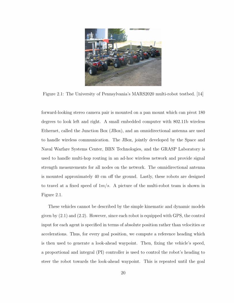
Figure 2.1: The University of Pennsylvania’s MARS2020 multi-robot testbed. [14]

forward-looking stereo camera pair is mounted on a pan mount which can pivot 180

degrees to look left and right. A small embedded computer with 802.11b wireless

Ethernet, called the Junction Box (JBox), and an omnidirectional antenna are used

to handle wireless communication. The JBox, jointly developed by the Space and

Naval Warfare Systems Center, BBN Technologies, and the GRASP Laboratory is

used to handle multi-hop routing in an ad-hoc wireless network and provide signal

strength measurements for all nodes on the network. The omnidirectional antenna

is mounted approximately 40 cm off the ground. Lastly, these robots are designed

to travel at a fixed speed of 1m/s. A picture of the multi-robot team is shown in

Figure 2.1.

These vehicles cannot be described by the simple kinematic and dynamic models

given by (2.1) and (2.2). However, since each robot is equipped with GPS, the control

input for each agent is specified in terms of absolute position rather than velocities or

accelerations. Thus, for every goal position, we compute a reference heading which

is then used to generate a look-ahead waypoint. Then, fixing the vehicle’s speed,

a proportional and integral (PI) controller is used to control the robot’s heading to

steer the robot towards the look-ahead waypoint. This is repeated until the goal

20

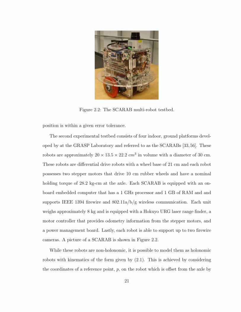
Figure 2.2: The SCARAB multi-robot testbed.

position is within a given error tolerance.

The second experimental testbed consists of four indoor, ground platforms devel-

oped by at the GRASP Laboratory and referred to as the SCARABs [33,56]. These

robots are approximately 20× 13.5× 22.2 cm3 in volume with a diameter of 30 cm.

These robots are differential drive robots with a wheel base of 21 cm and each robot

possesses two stepper motors that drive 10 cm rubber wheels and have a nominal

holding torque of 28.2 kg-cm at the axle. Each SCARAB is equipped with an on-

board embedded computer that has a 1 GHz processor and 1 GB of RAM and and

supports IEEE 1394 firewire and 802.11a/b/g wireless communication. Each unit

weighs approximately 8 kg and is equipped with a Hokuyo URG laser range finder, a

motor controller that provides odometry information from the stepper motors, and

a power management board. Lastly, each robot is able to support up to two firewire

cameras. A picture of a SCARAB is shown in Figure 2.2.

While these robots are non-holonomic, it is possible to model them as holonomic

robots with kinematics of the form given by (2.1). This is achieved by considering

the coordinates of a reference point, p, on the robot which is offset from the axle by

21

a distance of l and by translating the velocities of the reference point to commanded

linear and angular velocities, v and ω respectively, for the robot through the following

equations:

x

y

=

cos θ −l sin θ

sin θ l cos θ

v

ω

.Given a reference point p and a radius for a circle circumscribing the robot, which

we denote by r, this methodology ensures that all points on the robot lie within a

circle of radius l + r centered at p, enabling us to treat these vehicles as holonomic

circular robots with finite radius l + r.

2.2 Communications

Radio connectivity is often difficult to predict since it relies on complex propagation

mechanisms as well as other factors like the distance between the transmitter and

receiver, the three-dimensional geometry of the environment, and tranmission power.

As such, the received signal is often the sum of the various components resulting from

diffraction, scattering, reflection, transmission, and refraction of the transmitted

signal. Therefore, accurate prediction models must take into account the diverse

attenuation effects stemming from all these physical phenomena.

In the last few decades, the increase in demand of good quality and cost effective

radio systems has further emphasized the need of accurate models for predicting

radio propagation losses [62]. There are numerous prediction methods and models

in the literature today. In general, these propagation models can be categorized as

empirical, theoretical, or a combination of both. Empirical models implicitly take

into account all the environmental influences regardless of whether these can be

22

easily distinguished from one another. With enough data and tuning of the various

parameters, empirical models can often be quite accurate for a given environment.

The downside of these models, however, is that their quality is often dependent on

the accuracy of the measurements as well as the similarities between the environment

of interest and the environment where the measurements were made. Theoretical

models, on the other hand, are concerned with the physics of radio wave propagation

and are thus applicable to various different environments. However, implementations

of these models often require large databases of environmental characteristics which

can be very difficult to obtain. Additionally, given the large amount of data that

must be kept handy at all times, these models are often computationally inefficient

due to their complexity, which limits their use to mostly small outdoor environments.

While numerous models exist, they are often inadequate when applied to mobile

robot teams and/or sensor networks. This is because most existing models are ei-

ther a macrocell or a microcell propagation model. Macrocell propagation models

deal with systems whose transmission powers are in the tens of Watts and propa-

gation distances in the tens of kilometers. Under these circumstances, it is nearly

impossible to ensure line-of-sight between transmitters and receivers, and as such,

the signal propagates primarily by diffraction and reflection. Additionally, at these

scales, refraction from the atmosphere results in a significant contribution to propa-

gation loss. Microcell propagation models, on the other hand, deal with much smaller

outdoor regions, e.g. the area around a street corner. These models are generally

concerned with tranmission powers that are mostly in the milliWatt range, transmis-

sion distances ranging between 200 m to 1000 m, and base station antennae placed

approximately 3 m to 10 m above the ground. In these models, the surrounding

geometry plays a significant role when determining propagation losses.

Our work is primarily concerned with the deployment of teams of autonomous

23

robots that operate in urban environments. In these situations, radio paths are

relatively short in distance, roughly on the order of 10s or 100s of meters, with low

transmission powers. While microcell models provide an approximation, they are

often inadequate since these models generally assume fixed repeaters with antennae

approximately one to two stories above the ground, similar to mobile cell phone

networks and/or wireless data networks. On the other hand, the autonomous ground

vehicles under consideration are generally small, light-weight vehicles, often with

antennae no more than one to two feet off the ground. Under these circumstances,

ground effects such as reflection and scattering become the dominant propagation

mechanisms. As such, few, if any, existing propagation models actually match the

actual operating conditions of the robots in the field.

Despite these issues, the most common model used in the mobile robot litera-

ture [54, 86] to determine the signal strength, i.e. the measure of the strength of

a transmitted signal as it is received, is based on the following path loss or path

attenuation model:

PL = −20 log da · (1 + d/g)b + c

where PL denotes the path loss in dBµV/m, d denotes the distance to the trans-

mitting antenna, a is the basic attenuation rate for short distances often referred to

as the path loss exponent, b is the additional attenuation rate coefficient beyond the

breakpoint, g is the distance to the breakpoint, and c is a scaleable factor [37,85,90].

The path loss exponent typically ranges between 2, e.g. free space propagation, to

4, e.g. tunnel-like evironments. The breakpoint is the maximum distance before the

effects of diffraction becomes dominant with b ≈ 4.

There are many variations of the above model depending on the operating condi-

tions. For example, at distances less than the breakpoint, the model can be simplified

24

to

PL = −20 log da + c,

while at distances greater than the breakpoint, the model becomes

PL = −20 log d(a+b) + c.

In this work, outdoor experiments were conducted using a team of modified radio

controlled trucks equipped with omni-directional antennae that are no more than

two feet off the ground. Under these circumstances, the path loss exponent is closer

to 4. The interested reader is referred to [62] for further details.

2.3 Controllers

This work addresses the synthesis of controllers that can position a team of robots

along a desired boundary curve of a given shape while maintaining constraints with

other agents. In general, we assume each robot has the ability to localize itself within

some desired precision. Additionally, we assume each robot possesses a map of the

environment in which they are operating in, and, as such, potential function based

navigation strategies can be employed for navigation.

We rely on potential function based strategies to address the problem of coordi-

nating large numbers of robots. The main advantage of potential based methods is

that they allow us to simultaneously solve the path planning and control problems

simultaneously. In practice, however, these approaches require robots to have precise

localization capabilities to ensure continuity of the feedback policy. In this work, we

assume robots have either well-defined safe zones or repulsion zones to ensure col-

lision avoidance. As such, given the limitations of the hardware, it is possible for

25

us to limit computational errors in our potential function strategies resulting from

inaccurate estimation of robots’ positions by appropriately selecting these safety

zones.

Since our focus is on the coordination of large teams of robots, as such, we are

concerned with feedback controllers that are decentralized, simple to implement, and

identical across all agents, thus enabling scalability as the size of the team increases.

While each robot is equipped with a wireless communication module, we assume

no state information is exchanged among the agents. Rather, the positions of each

robot’s neighbors are inferred using range and bearing sensors. In the event a robot

must infer a neighbor’s velocity, we assume the robot is capable of doing so from

its existing sensor suite, i.e. filtering position history information for each neighbor,

rather than assume the presence of communication. Lastly, in certain special cases,

we will assume each robot has the ability to detect failed agents within its sensing

vicinity. Depending on the severity of the failure, in practice, this can be achieved

via minimal communication between the failed robot and the live ones, or through

the use of a bump sensor, and/or some high-level reasoning capabilities.

26

Chapter 3

Maintaining Network Connectivity

and Performance in Robot Teams

We consider the problem of a team of robots operating in an urban, potentially

hazardous, environment for tasks such as reconnaissance and perimeter surveillance,

where maintaining team connectivity is essential for situational awareness. In these

tasks, robots must have the ability to align themselves along the boundaries of com-

plex shapes in two dimensions while ensuring the successful transmission of critical

data. Importantly, navigation based solely on the geometry of the environment will

not always guarantee a connected communication network. In these situations, a

rough model of the radio signal propagation encoded in a radio connectivity map,

i.e. a map that gives the average signal strength measurements from one position

in the workspace to any other position, becomes extremely helpful in the planning

phase. Furthermore, since real-world environments are often very complex and dy-

namic, it is important for robots to also have the ability to respond to real-time

changes in link quality to ensure network connectivity.

Figure 1.1 shows actual signal strength measurements obtained in an environment

27

representative of an urban park using two nodes at different separation distances.

Although, there is a strong correlation between signal strength and distance, there is

also a lot of variability due to the various factors mentioned earlier [62]. These kinds

of information cannot always be accurately inferred from a radio connectivity map.

Thus, successful mission execution will require both proper deliberative planning

and suitably designed reactive behaviors to facilitate the operation of the team with

little to no direct human supervision.

Most prior works in the area of communication link maintenance leave the bur-

den of performance specification to fixed metrics, typically based on the distance

between nodes or on simulated signal strength. However, as mentioned earlier, radio

signal propagation depends on a variety of factors that are often difficult to capture

in simulation alone. Rather than rely on simulation, our approach entails the use

of radio connectivity maps for planning as well as low level reactive controllers that

respond to changes in actual signal strength or verified network bandwidth. The

goal is to develop strategies that exploit information gathered during an initial ex-

ploration phase coupled with well-designed reactive behaviors that remain minimally

disruptive to any high level deliberative plans in order to maximize the team’s ability

to provide effective situational awareness to a base station. In essence, our strategies

are based on metrics that do not rely on assumptions that may not be transferable

or realistic in the physical workspace that the team is operating within.

This chapter presents experimentally verified strategies for maintenance of point-

to-point communication links in multi-robot teams. Section 3.1 begins with the

presentation of a methodology to enable a team of robots to obtain signal strength

information used to populate a radio signal strength map for an urban environment.

Next, Section 3.2 presents low-level reactive controllers that can be used to constrain

the motion of individual agents based on two link quality measures: signal strength

28

and perceived network bandwidth. We present two sets of experimental results us-

ing these controllers in outdoor environments under different network interconnection

topologies. In the first set of experiments, the radio connectivity map was used to

determine a deployment strategy for a reconnaissance task. In the second set of

experiments, we deployed our multi-robot team to execute a perimeter surveillance

task. The reactive controllers are designed to be minimally disruptive to the over-

all deliberative plan, and provide situational awareness to a base station including

notification regarding potential failure points in the communication network.

3.1 Multi-robot Radio Mapping

This section describes a methodology to generate a deployment strategy which en-

ables a homogeneous team of mobile-robots to obtain a radio connectivity map for

an urban environment. Specifically, the methodology is described for two special

cases: i) when the team consists of two robots, and ii) when the team consists of

three robots. Experimental results obtained using a three-robot team are presented.

3.1.1 Modeling

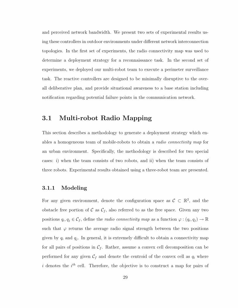
For any given environment, denote the configuration space as C ⊂ R2, and the

obstacle free portion of C as Cf , also referred to as the free space. Given any two

positions qi, qj ∈ Cf , define the radio connectivity map as a function ϕ : (qi, qj)→ R

such that ϕ returns the average radio signal strength between the two positions

given by qi and qj. In general, it is extremely difficult to obtain a connectivity map

for all pairs of positions in Cf . Rather, assume a convex cell decomposition can be

performed for any given Cf and denote the centroid of the convex cell as qi where

i denotes the ith cell. Therefore, the objective is to construct a map for pairs of

29

locations in the set Q = q1, . . . , qn1 where Q is a subset of Cf .

While it is reasonable to assume a convex decomposition exists for any given

Cf , it does not necessarily mean that the signal strength for all pairs of positions

in any two cells will be the same. However, since each cell is convex, any two

positions within the same cell will have line-of-sight, thus making it possible to

predict the signal strength for the pair given prior knowledge of the variation of

radio signal transmission characteristics with distance. Since the objective is to

develop a methodology for the construction of the radio connectivity map rather

than determining the appropriate cell decomposition, it will be assumed that the

decomposition is given.

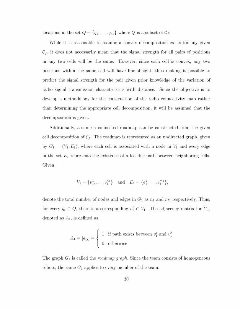
Additionally, assume a connected roadmap can be constructed from the given

cell decomposition of Cf . The roadmap is represented as an undirected graph, given

by G1 = (V1, E1), where each cell is associated with a node in V1 and every edge

in the set E1 represents the existence of a feasible path between neighboring cells.

Given,

V1 = v11, . . . , v

n11 and E1 = e1

1, . . . , em11 ,

denote the total number of nodes and edges in G1 as n1 and m1 respectively. Thus,

for every qi ∈ Q, there is a corresponding vi1 ∈ V1. The adjacency matrix for G1,

denoted as A1, is defined as

A1 = [aij] =

1 if path exists between vi1 and vj1

0 otherwise

The graph G1 is called the roadmap graph. Since the team consists of homogeneous

robots, the same G1 applies to every member of the team.

30

Next, define the radiomap graph, R = (V1, L1), such that R is used to encode

the signal strength information one would like to gather. The edge set L1 represents

signal strength measurements that must be obtained for pairs of nodes and is selected

a priori based on the task objectives, the physical environment, prior knowledge of

radio signal transmission characteristics, and may include all possible edges in G1.

The adjacency matrix AR for the radiomap graph, R, is then given by

AR = [aRij ] =

1 if signal strength between vi1

and vj1 is to be measured

0 otherwise

Given the roadmap and radiomap graphs, G1 and R, denote the multi-robot

exploration graph as Gk = (Vk, Ek), where k denotes the number of robots in the

team. The graph Gk is then constructed such that obtaining an optimal deployment

strategy for measuring the edges in L1 is equivalent to solving for a shortest path on

the graph Gk. The methodology is presented in the following section with special

attention paid to the two and three robot cases.

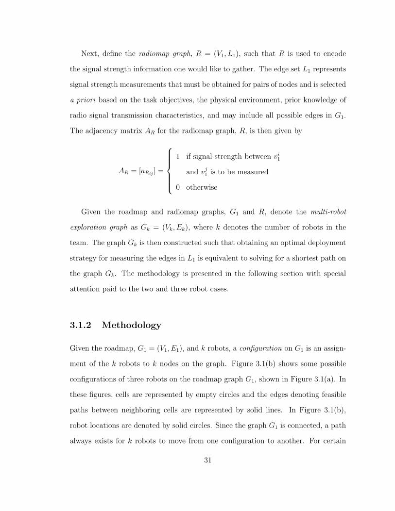
3.1.2 Methodology

Given the roadmap, G1 = (V1, E1), and k robots, a configuration on G1 is an assign-

ment of the k robots to k nodes on the graph. Figure 3.1(b) shows some possible

configurations of three robots on the roadmap graph G1, shown in Figure 3.1(a). In

these figures, cells are represented by empty circles and the edges denoting feasible

paths between neighboring cells are represented by solid lines. In Figure 3.1(b),

robot locations are denoted by solid circles. Since the graph G1 is connected, a path

always exists for k robots to move from one configuration to another. For certain

31

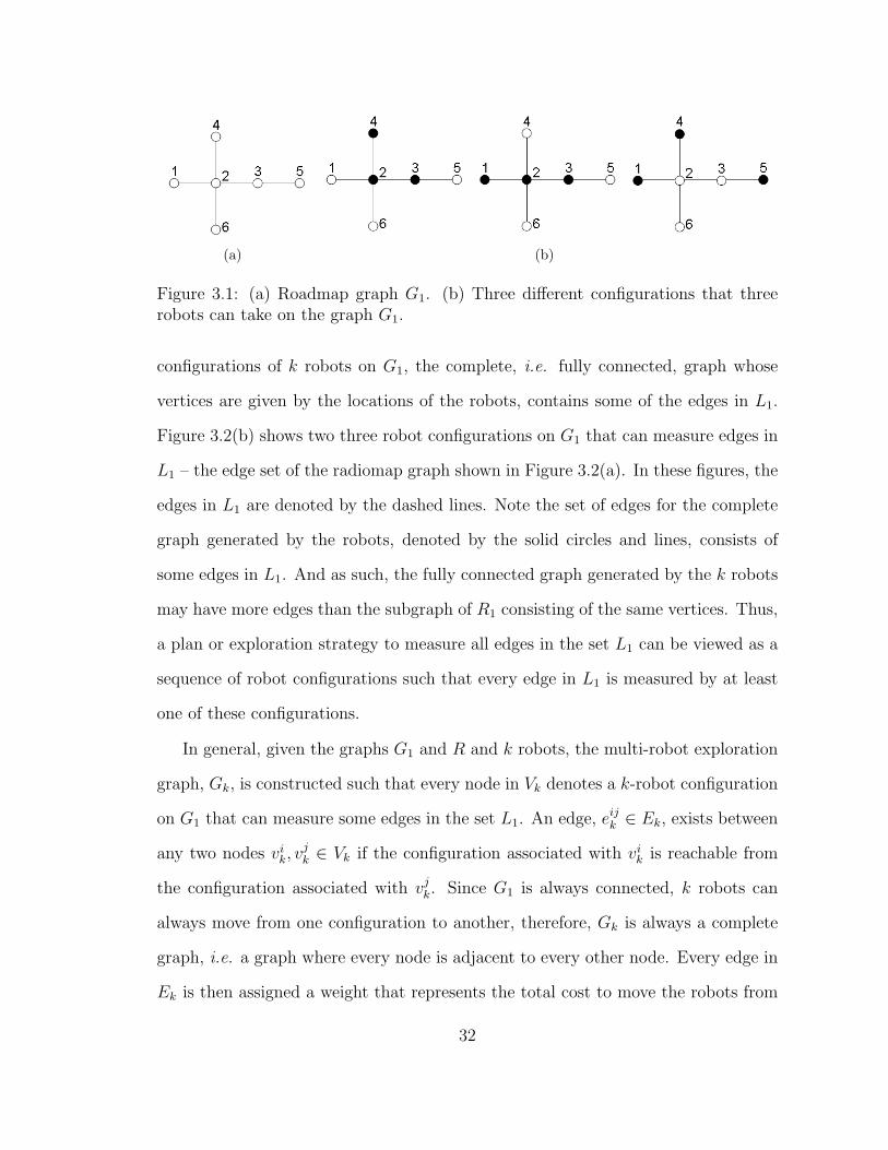
(a) (b)

Figure 3.1: (a) Roadmap graph G1. (b) Three different configurations that threerobots can take on the graph G1.

configurations of k robots on G1, the complete, i.e. fully connected, graph whose

vertices are given by the locations of the robots, contains some of the edges in L1.

Figure 3.2(b) shows two three robot configurations on G1 that can measure edges in

L1 – the edge set of the radiomap graph shown in Figure 3.2(a). In these figures, the

edges in L1 are denoted by the dashed lines. Note the set of edges for the complete

graph generated by the robots, denoted by the solid circles and lines, consists of

some edges in L1. And as such, the fully connected graph generated by the k robots

may have more edges than the subgraph of R1 consisting of the same vertices. Thus,

a plan or exploration strategy to measure all edges in the set L1 can be viewed as a

sequence of robot configurations such that every edge in L1 is measured by at least

one of these configurations.

In general, given the graphs G1 and R and k robots, the multi-robot exploration

graph, Gk, is constructed such that every node in Vk denotes a k-robot configuration

on G1 that can measure some edges in the set L1. An edge, eijk ∈ Ek, exists between

any two nodes vik, vjk ∈ Vk if the configuration associated with vik is reachable from

the configuration associated with vjk. Since G1 is always connected, k robots can

always move from one configuration to another, therefore, Gk is always a complete

graph, i.e. a graph where every node is adjacent to every other node. Every edge in

Ek is then assigned a weight that represents the total cost to move the robots from

32

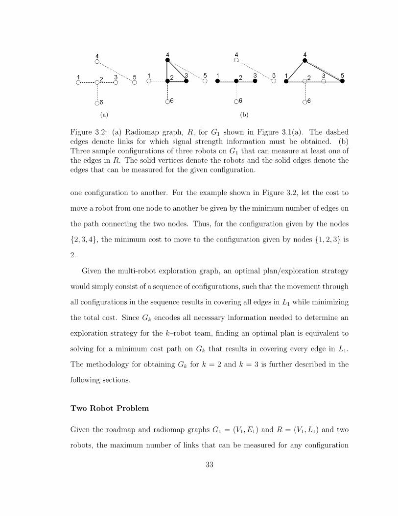
(a) (b)

Figure 3.2: (a) Radiomap graph, R, for G1 shown in Figure 3.1(a). The dashededges denote links for which signal strength information must be obtained. (b)Three sample configurations of three robots on G1 that can measure at least one ofthe edges in R. The solid vertices denote the robots and the solid edges denote theedges that can be measured for the given configuration.

one configuration to another. For the example shown in Figure 3.2, let the cost to

move a robot from one node to another be given by the minimum number of edges on

the path connecting the two nodes. Thus, for the configuration given by the nodes

2, 3, 4, the minimum cost to move to the configuration given by nodes 1, 2, 3 is

2.

Given the multi-robot exploration graph, an optimal plan/exploration strategy

would simply consist of a sequence of configurations, such that the movement through

all configurations in the sequence results in covering all edges in L1 while minimizing

the total cost. Since Gk encodes all necessary information needed to determine an

exploration strategy for the k–robot team, finding an optimal plan is equivalent to

solving for a minimum cost path on Gk that results in covering every edge in L1.

The methodology for obtaining Gk for k = 2 and k = 3 is further described in the

following sections.

Two Robot Problem

Given the roadmap and radiomap graphs G1 = (V1, E1) and R = (V1, L1) and two

robots, the maximum number of links that can be measured for any configuration

33

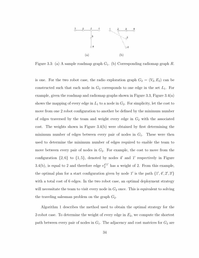
(a) (b)

Figure 3.3: (a) A sample roadmap graph G1. (b) Corresponding radiomap graph R.

is one. For the two robot case, the radio exploration graph G2 = (V2, E2) can be

constructed such that each node in G2 corresponds to one edge in the set L1. For

example, given the roadmap and radiomap graphs shown in Figure 3.3, Figure 3.4(a)

shows the mapping of every edge in L1 to a node in G2. For simplicity, let the cost to

move from one 2 robot configuration to another be defined by the minimum number

of edges traversed by the team and weight every edge in G2 with the associated

cost. The weights shown in Figure 3.4(b) were obtained by first determining the

minimum number of edges between every pair of nodes in G1. These were then

used to determine the minimum number of edges required to enable the team to

move between every pair of nodes in G2. For example, the cost to move from the

configuration 2, 6 to 1, 5, denoted by nodes 4′ and 1′ respectively in Figure

3.4(b), is equal to 2 and therefore edge e4′1′2 has a weight of 2. From this example,

the optimal plan for a start configuration given by node 1′ is the path 1′, 4′, 2′, 3′

with a total cost of 6 edges. In the two robot case, an optimal deployment strategy

will necessitate the team to visit every node in G2 once. This is equivalent to solving

the traveling salesman problem on the graph G2.

Algorithm 1 describes the method used to obtain the optimal strategy for the

2-robot case. To determine the weight of every edge in E2, we compute the shortest

path between every pair of nodes in G1. The adjacency and cost matrices for G2 are

34

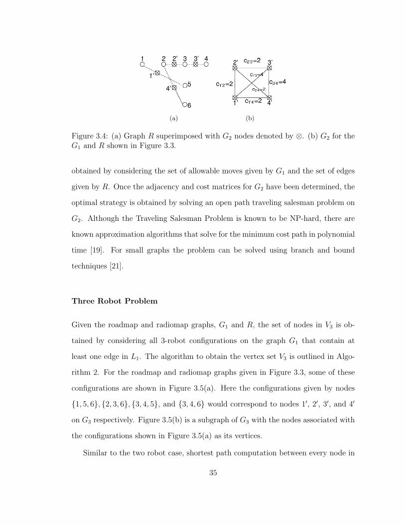
(a) (b)

Figure 3.4: (a) Graph R superimposed with G2 nodes denoted by ⊗. (b) G2 for theG1 and R shown in Figure 3.3.

obtained by considering the set of allowable moves given by G1 and the set of edges

given by R. Once the adjacency and cost matrices for G2 have been determined, the

optimal strategy is obtained by solving an open path traveling salesman problem on

G2. Although the Traveling Salesman Problem is known to be NP-hard, there are

known approximation algorithms that solve for the minimum cost path in polynomial

time [19]. For small graphs the problem can be solved using branch and bound

techniques [21].

Three Robot Problem

Given the roadmap and radiomap graphs, G1 and R, the set of nodes in V3 is ob-

tained by considering all 3-robot configurations on the graph G1 that contain at

least one edge in L1. The algorithm to obtain the vertex set V3 is outlined in Algo-

rithm 2. For the roadmap and radiomap graphs given in Figure 3.3, some of these

configurations are shown in Figure 3.5(a). Here the configurations given by nodes

1, 5, 6, 2, 3, 6, 3, 4, 5, and 3, 4, 6 would correspond to nodes 1′, 2′, 3′, and 4′

on G3 respectively. Figure 3.5(b) is a subgraph of G3 with the nodes associated with

the configurations shown in Figure 3.5(a) as its vertices.

Similar to the two robot case, shortest path computation between every node in

35

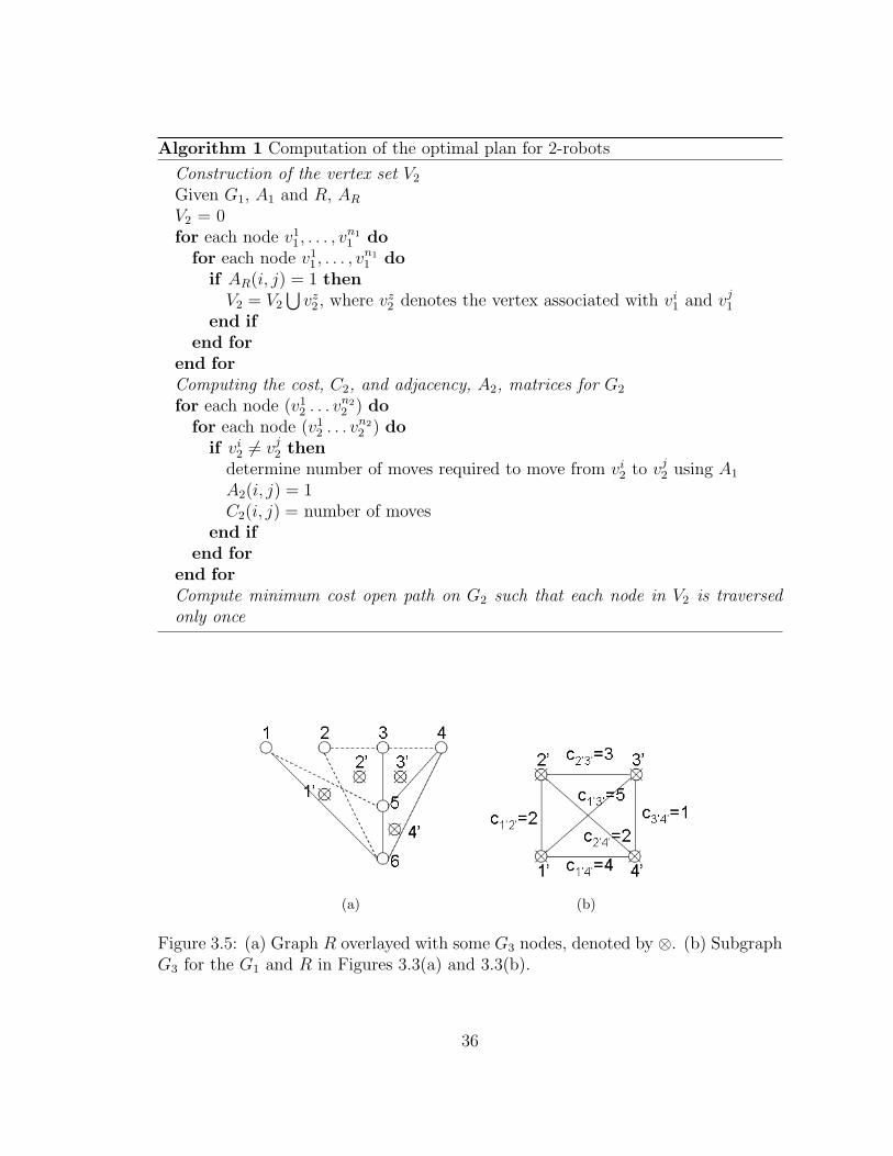
Algorithm 1 Computation of the optimal plan for 2-robots

Construction of the vertex set V2

Given G1, A1 and R, ARV2 = 0for each node v1

1, . . . , vn11 do

for each node v11, . . . , v

n11 do

if AR(i, j) = 1 thenV2 = V2

⋃vz2, where vz2 denotes the vertex associated with vi1 and vj1

end ifend for

end forComputing the cost, C2, and adjacency, A2, matrices for G2

for each node (v12 . . . v

n22 ) do

for each node (v12 . . . v

n22 ) do

if vi2 6= vj2 thendetermine number of moves required to move from vi2 to vj2 using A1

A2(i, j) = 1C2(i, j) = number of moves

end ifend for

end forCompute minimum cost open path on G2 such that each node in V2 is traversedonly once

(a) (b)

Figure 3.5: (a) Graph R overlayed with some G3 nodes, denoted by ⊗. (b) SubgraphG3 for the G1 and R in Figures 3.3(a) and 3.3(b).

36

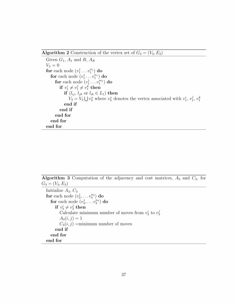
Algorithm 2 Construction of the vertex set of G3 = (V3, E3)

Given G1, A1 and R, ARV3 = 0for each node (v1

1 . . . vn11 ) do

for each node (v11 . . . v

n11 ) do

for each node (v11 . . . v

m11 ) do

if vi1 6= vj1 6= vk1 thenif (lij, ljk or lik ∈ L1) thenV3 = V3

⋃vx3 where vx3 denotes the vertex associated with vi1, vj1, vk1

end ifend if

end forend for

end for

Algorithm 3 Computation of the adjacency and cost matrices, A3 and C3, forG3 = (V3, E3)

Initialize A3, C3

for each node (v13, . . . v

n33 ) do

for each node (v13, . . . v

n33 ) do

if vi3 6= vj3 thenCalculate minimum number of moves from vi3 to vj3A3(i, j) = 1C3(i, j) =minimum number of moves

end ifend for

end for

37

G1 is required to determine the weight of every edge in E3. For the three robot case,

every edge in the set L1 may potentially be associated with more than one node

in V3. Thus, the optimal plan for the three robot case would result in a path that

contains a subset of the nodes in V3. For this example, an optimal plan starting

at the configuration given by node 1′ is the path 1′, 2′, 4′ with a total cost of 4,

and does not contain node 3′. In general, given a starting node on G3, a greedy

algorithm is used to compute a path on G3 such that traversal of each node on the

path increases the number of measured edges in L1. Thus, at any configuration, the

next configuration chosen is the one that increases the number of edges measured

in L1 and requires the least amount of moves to reach. During execution, robots

are allowed to cross each other as they switch from one configuration to another

since inter-robot collisions can be prevented via each robot’s local obstacle avoidance

routines.

3.1.3 Experimental Setup and Results

The objective of this experiment was to deploy a team of three robots to obtain a

radio signal strength map for the Military Operations on Urban Terrain (MOUT)

training site, located in Ft. Benning, Georgia, where radio signal strength data

is important for operations such as surveillance, reconnaissance, and search and

rescue. Figure 3.6(a) is an aerial surveillance picture of the MOUT site. The image

was obtained using a fixed wing UAV taken at an altitude of 150 meters. The

area shown is approximately 90 × 120 squared meters. More information on the

experiments conducted at the MOUT site can be found in [15,35,36].

38

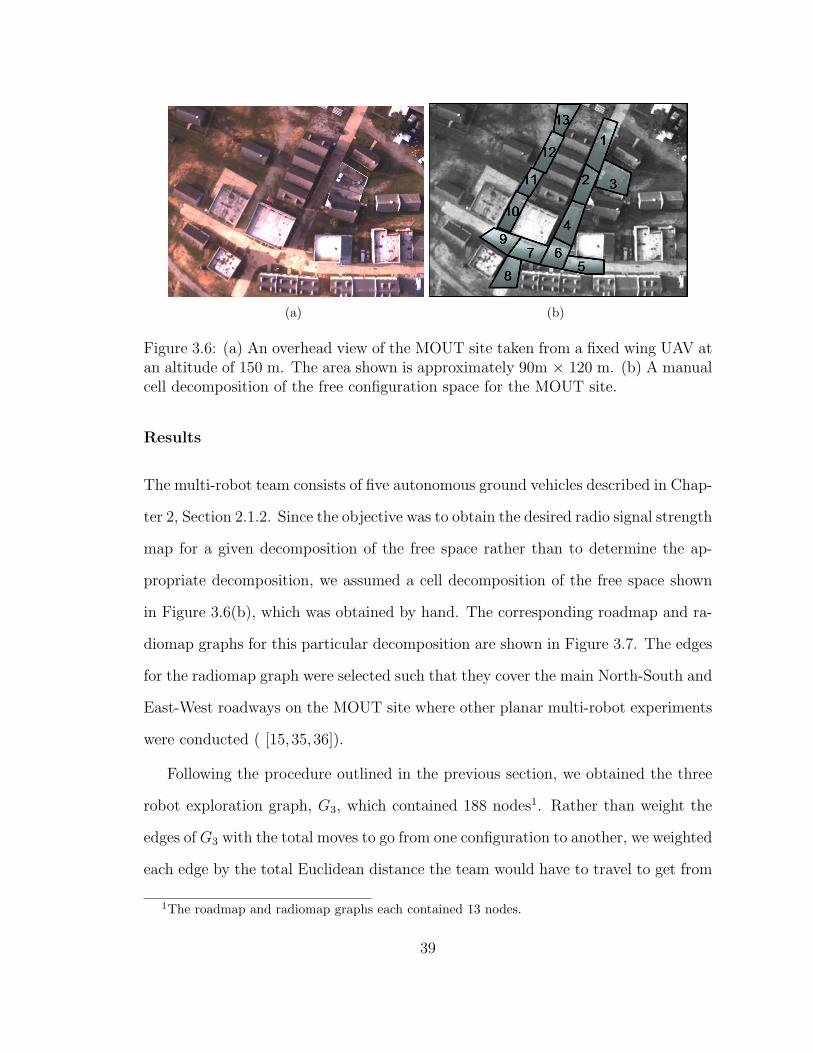
(a) (b)

Figure 3.6: (a) An overhead view of the MOUT site taken from a fixed wing UAV atan altitude of 150 m. The area shown is approximately 90m × 120 m. (b) A manualcell decomposition of the free configuration space for the MOUT site.

Results

The multi-robot team consists of five autonomous ground vehicles described in Chap-

ter 2, Section 2.1.2. Since the objective was to obtain the desired radio signal strength

map for a given decomposition of the free space rather than to determine the ap-

propriate decomposition, we assumed a cell decomposition of the free space shown

in Figure 3.6(b), which was obtained by hand. The corresponding roadmap and ra-

diomap graphs for this particular decomposition are shown in Figure 3.7. The edges

for the radiomap graph were selected such that they cover the main North-South and

East-West roadways on the MOUT site where other planar multi-robot experiments

were conducted ( [15,35,36]).

Following the procedure outlined in the previous section, we obtained the three

robot exploration graph, G3, which contained 188 nodes1. Rather than weight the

edges of G3 with the total moves to go from one configuration to another, we weighted

each edge by the total Euclidean distance the team would have to travel to get from

1The roadmap and radiomap graphs each contained 13 nodes.

39

one configuration to another to more accurately capture the cost associated with each

configuration change. The starting configuration for the 3-robot team was selected

to be at nodes 1, 2, 3 in Figure 3.7. The exploration strategy that was obtained

would deploy the robot team in the following sequence: 1, 2, 3, 1, 2, 4, 2, 3, 4,

4, 5, 6, 6, 7, 9, 6, 8, 9, 7, 8, 9, 9, 10, 11, 10, 11, 12, and 11, 12, 13.

Once this strategy was obtained, a centrally located waypoint was selected for

each cell and each robot was then assigned a set of waypoints to be traversed based on

the exploration strategy. Using GPS, the robots navigated to each of their assigned

locations. Upon arrival at each waypoint, the robots would synchronize and measure

their signal strengths to other team members. If the synchronization failed, each

robot would move on towards the next waypoint on its assigned list. To enable each

robot to return to its starting position after completion, we assigned each robot its

starting position as its last waypoint. The waypoints and cell decompositions were

manually chosen to minimize the number of failed synchronizations during execution

based on prior knowledge of the variation of signal strength with distance (See Figure

1.1). In addition, each robot was continuously logging both signal strength and

position data such that in the event of a failed synchronization the information

could be retrieved. There were no synchronization failures during the experiment.

Figure 3.8 shows the radio signal strength map constructed for the MOUT site.

The numbers by each edge are the averaged normalized signal strength measurements

obtained by the robots located at each pair of positions. On average the GPS errors

ranged from 2−3 meters to as much as 5 meters. However, the robots were generally

able to stay within the boundaries of the convex cells.

40

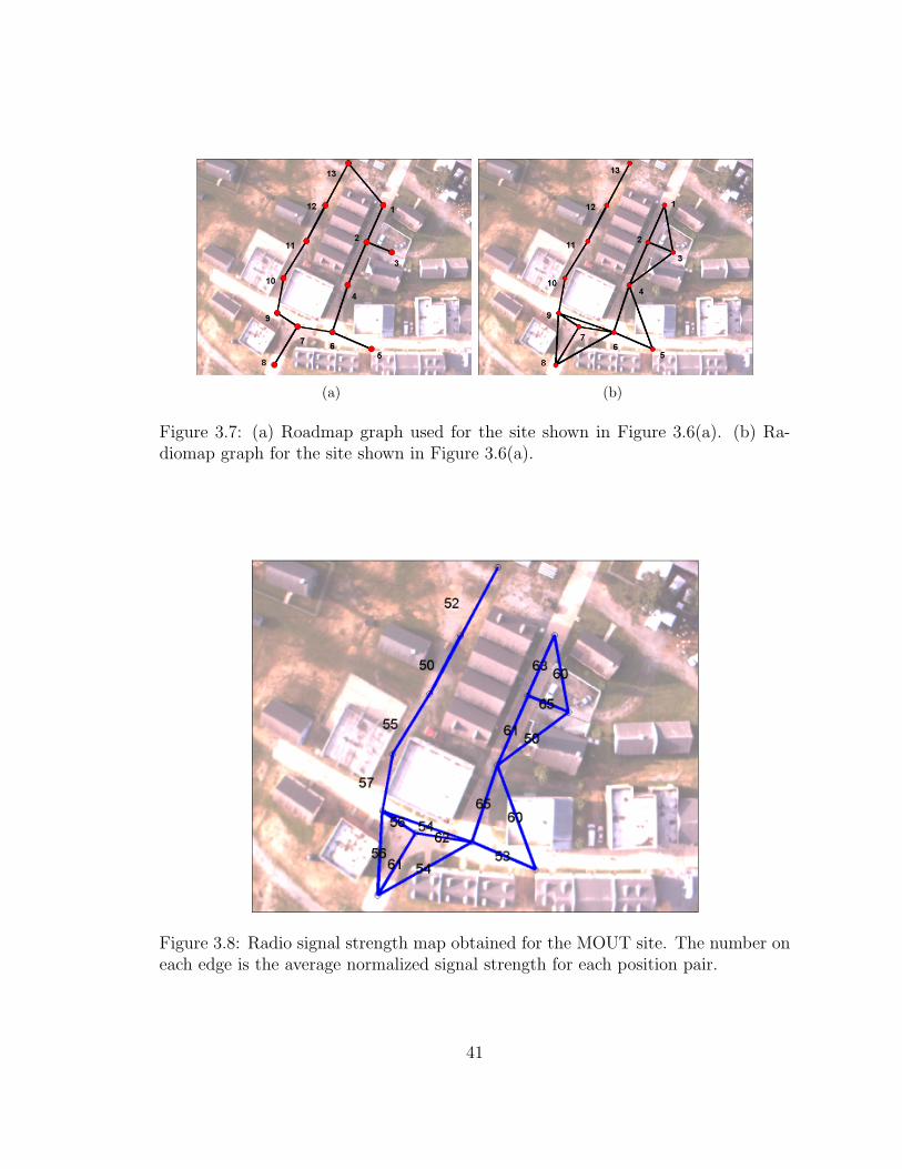
(a) (b)

Figure 3.7: (a) Roadmap graph used for the site shown in Figure 3.6(a). (b) Ra-diomap graph for the site shown in Figure 3.6(a).

Figure 3.8: Radio signal strength map obtained for the MOUT site. The number oneach edge is the average normalized signal strength for each position pair.

41

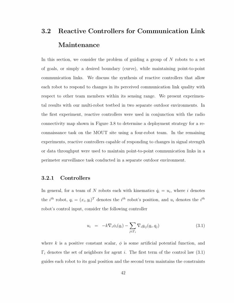
3.2 Reactive Controllers for Communication Link

Maintenance

In this section, we consider the problem of guiding a group of N robots to a set

of goals, or simply a desired boundary (curve), while maintaining point-to-point

communication links. We discuss the synthesis of reactive controllers that allow

each robot to respond to changes in its perceived communication link quality with

respect to other team members within its sensing range. We present experimen-

tal results with our multi-robot testbed in two separate outdoor environments. In

the first experiment, reactive controllers were used in conjunction with the radio

connectivity map shown in Figure 3.8 to determine a deployment strategy for a re-

connaissance task on the MOUT site using a four-robot team. In the remaining

experiments, reactive controllers capable of responding to changes in signal strength

or data throughput were used to maintain point-to-point communication links in a

perimeter surveillance task conducted in a separate outdoor environment.

3.2.1 Controllers

In general, for a team of N robots each with kinematics qi = ui, where i denotes

the ith robot, qi = (xi, yi)T denotes the ith robot’s position, and ui denotes the ith

robot’s control input, consider the following controller

ui = −k∇iφi(qi)−∑j∈Γi

∇igij(qi, qj) (3.1)

where k is a positive constant scalar, φ is some artificial potential function, and

Γi denotes the set of neighbors for agent i. The first term of the control law (3.1)

guides each robot to its goal position and the second term maintains the constraints

42

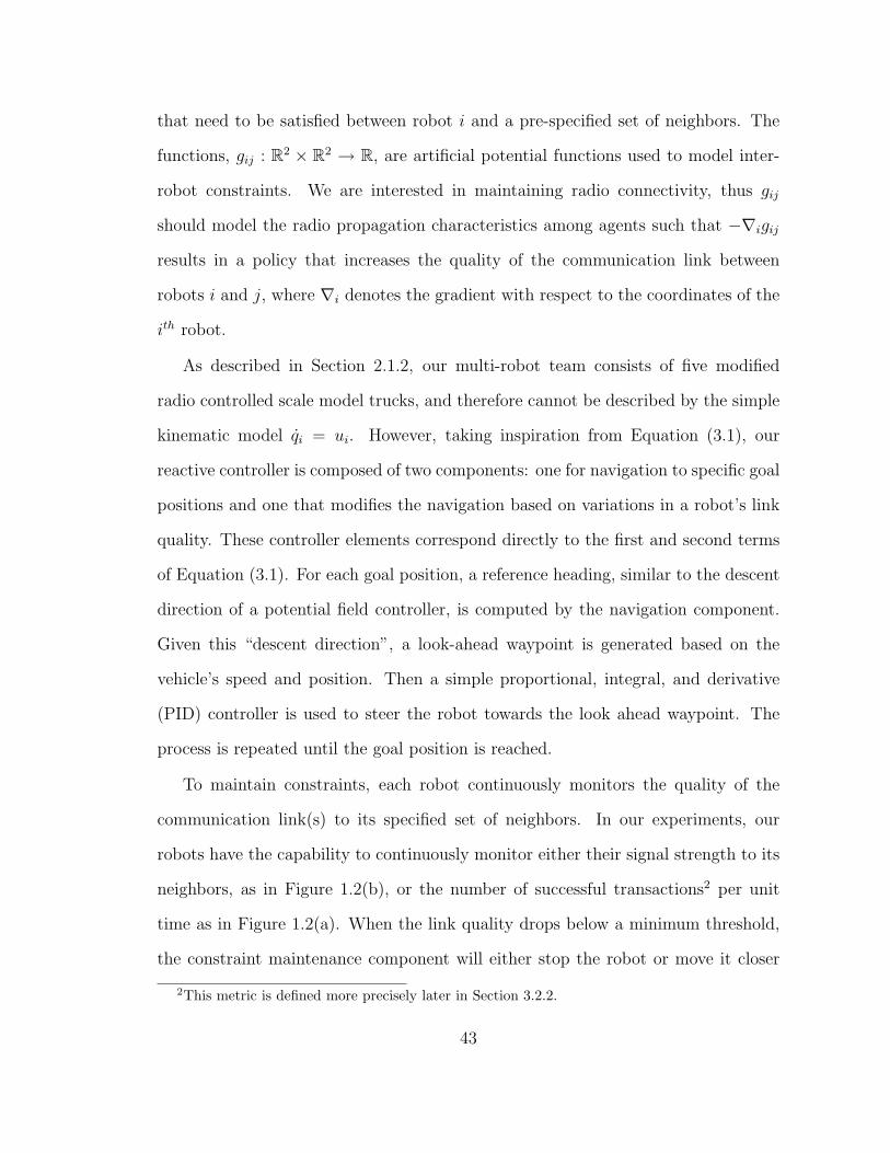
that need to be satisfied between robot i and a pre-specified set of neighbors. The

functions, gij : R2 × R2 → R, are artificial potential functions used to model inter-

robot constraints. We are interested in maintaining radio connectivity, thus gij

should model the radio propagation characteristics among agents such that −∇igij

results in a policy that increases the quality of the communication link between

robots i and j, where ∇i denotes the gradient with respect to the coordinates of the

ith robot.

As described in Section 2.1.2, our multi-robot team consists of five modified

radio controlled scale model trucks, and therefore cannot be described by the simple

kinematic model qi = ui. However, taking inspiration from Equation (3.1), our

reactive controller is composed of two components: one for navigation to specific goal

positions and one that modifies the navigation based on variations in a robot’s link

quality. These controller elements correspond directly to the first and second terms

of Equation (3.1). For each goal position, a reference heading, similar to the descent

direction of a potential field controller, is computed by the navigation component.

Given this “descent direction”, a look-ahead waypoint is generated based on the

vehicle’s speed and position. Then a simple proportional, integral, and derivative

(PID) controller is used to steer the robot towards the look ahead waypoint. The

process is repeated until the goal position is reached.

To maintain constraints, each robot continuously monitors the quality of the

communication link(s) to its specified set of neighbors. In our experiments, our

robots have the capability to continuously monitor either their signal strength to its

neighbors, as in Figure 1.2(b), or the number of successful transactions2 per unit

time as in Figure 1.2(a). When the link quality drops below a minimum threshold,

the constraint maintenance component will either stop the robot or move it closer

2This metric is defined more precisely later in Section 3.2.2.

43

to its neighbor until the quality returns to an acceptable level. When stopped, a

robot can wait for a specified time interval before attempting to move towards its

goal again. If the stopped robot perceives an increase in its link quality above the

acceptable level, it can once again attempt to move towards its goal. Such recovery

measures may be used to lessen the times a robot is caught in a spatio-temporal dip

in link quality due to dynamic changes in the environment. In other words, local

minima situations, in which a robot stopped before reaching its goal, caused by some

temporary interference in the environment. Additionally, these measures also ensure

that a robot is constantly minimizing its distance to the goal as long as all constraints

are satisfied. We have purposefully incorporated these recovery measures in some of

our experiments to highlight the reactive nature of our controller. The algorithm is

summarized in Algorithm 4. In this algorithm, the “Recover” behavior drives the

robot closer to the neighbor it is attempting to maintain its link quality with. While

we chose a binary signal derived from the link quality to control the robots since

they are designed to travel at a constant fixed speed, there is an effective deadband

in the controller given by the “Minimum” and “Acceptable” quality thresholds in

Algorithm 4.

By design, our reactive controller favors constraint satisfaction above reaching the

goal position. This is to ensure that the quality of the communication link is always

maintained, thus providing a human operator at a remote base station the ability

to monitor the various communication links in the network. At the base station,

display panels with each robot’s imagery data and/or the signal strength measured

by the various team members can be displayed. In the event the Base did not receive

new data from a particular robot, or should some particular link exhibit low signal

strength, an indication of the detected failure is relayed to the human operator. This

capability, possible because the team always remains connected, enables the operator

44

Algorithm 4 Link Quality Constrained Navigation

if LinkQuality < Minimum thenRecover;recover flag = true;

end ifif Minimum < LinkQuality ≤ Acceptable then

if recover flag thenStop and wait;recover flag = false;stopped = true;waitTime = current time;

end ifif (current time - waitTime) > MaxWaitTime then

Retry going to goal;stopped = false;

end ifend ifif LinkQuality > Acceptable then

Go to goal;end if

to decide whether or not to deploy additional robots, or to re-organize the team.

3.2.2 Link Quality Estimation

Signal strength between a sender and a receiver is a function of the transmission

power, antenna gains, and signal attenuation. Our robots are equipped with JBoxes

that, among other things, provide signal strength measurements to every node on

the network. We refer the interested reader to [89] and [75] for operational details

on the JBox.

In contrast, it is difficult for an individual robot to estimate the available band-

width at any given point in time since bandwidth is a function of the number of

nodes, the amount of traffic on the network, as well as the signal strength. In multi-

robot applications, it is often relevant to talk about bandwidth in terms of units

45

of application level data that can be transmitted, therefore we define a successful

transaction to be the transmission of one unit of application level data sent by a

sender with an acknowledgment of receipt sent by the receiver. A robot’s conserva-

tive estimate of available bandwidth is determined based on the number of successful

transactions it achieves over some interval of time.

For our experimental setup, we set one unit of application level data equal to

a JPEG image of approximately 10 KB in size. We define a successful transaction

to be the transmission of such an image by the sender followed by the receipt of

acknowledgment sent by the receiver. Then, based on the desired transaction rate,

i.e. number of successful transactions per time interval, the robot, i.e. the sender,

will periodically evaluate its connection with the receiver. The available bandwidth

controller comprises two stages of response: network usage throttling, and robot re-

positioning corresponding to the “Recover” behavior in Algorithm 4. A robot that is

streaming data over the network is capable of detecting when a network connection

is not keeping up with the load being put on it, i.e. when some messages are

dropped due to a full send buffer. When this type of application–level packet loss is

detected, the system will automatically throttle communication over this particular

network link until a prescribed threshold is hit. This threshold is determined based

on mission specifications; we typically specified video at a rate of three frames-per-

second as a requirement because this was a realistic target for the 802.11b hardware in

use, and provided sufficient video coverage to convey situational awareness. When

the network throttling mechanism bumps into the lower threshold, the controller

subsumes position control to move the robot closer to the peer it is attempting to

communicate with. This action serves to increase signal strength, which reduces the

number of low-level transmission retries caused by noise or attenuation.

All throughput estimation in this framework is conservative; we do not attempt

46

to measure maximum data rates available on the network, but rather we verify

that some prescribed minimum data throughput rate is available. This approach

minimizes the amount of network traffic related solely to throughput measurement,

and instead leverages throughput assessment on normal data traffic when such traffic

satisfies the constraint. When normal traffic is not of sufficient volume to verify

that the minimum available bandwidth constraint is met, a connection monitor will

periodically verify available throughput. This latter mechanism, which simply sends

data at a rate that verifies constraint satisfaction for a short period of time, allows

us to deploy robots that do not maintain consistent data flow back to the base

station, e.g. robots that only send event data, yet still be confident that the available

throughput would likely be available if it should be needed.

3.2.3 Experimental Results

In this section we present three sets of experimental results. The first experiment

was conducted at the MOUT site, shown in Figure 3.6(a). This experiment was

modeled after a reconnaissance application where the objective was to deploy a team

of four robots to obtain surveillance imagery at a designated location out of line-

of-sight and single-hop radio communication range with the base station. In this

experiment we used information gleaned from our radio connectivity map, shown

in Figure 3.8, to determine the deployment strategy, and coupled this with low

level reactive controllers to enable the team to respond to unforeseen changes in

signal strength. The second and third sets of experiments were conducted at one

of the University of Pennsylvania’s soccer fields. A satellite image and a schematic

of its surroundings are shown in Figure 3.9. These experiments were based on a

perimeter surveillance application in which each robot was required to send imagery

47

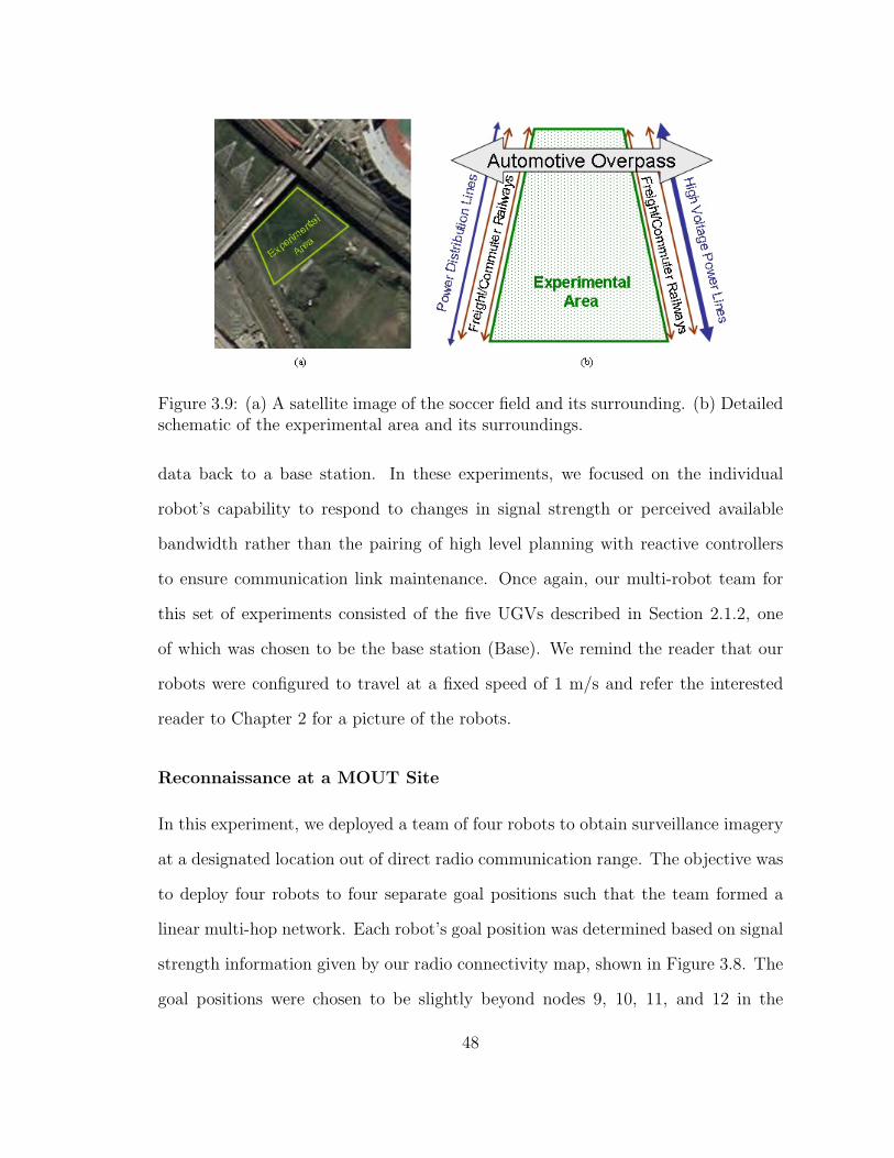
Figure 3.9: (a) A satellite image of the soccer field and its surrounding. (b) Detailedschematic of the experimental area and its surroundings.

data back to a base station. In these experiments, we focused on the individual

robot’s capability to respond to changes in signal strength or perceived available

bandwidth rather than the pairing of high level planning with reactive controllers

to ensure communication link maintenance. Once again, our multi-robot team for

this set of experiments consisted of the five UGVs described in Section 2.1.2, one

of which was chosen to be the base station (Base). We remind the reader that our

robots were configured to travel at a fixed speed of 1 m/s and refer the interested

reader to Chapter 2 for a picture of the robots.

Reconnaissance at a MOUT Site

In this experiment, we deployed a team of four robots to obtain surveillance imagery

at a designated location out of direct radio communication range. The objective was

to deploy four robots to four separate goal positions such that the team formed a

linear multi-hop network. Each robot’s goal position was determined based on signal

strength information given by our radio connectivity map, shown in Figure 3.8. The

goal positions were chosen to be slightly beyond nodes 9, 10, 11, and 12 in the

48

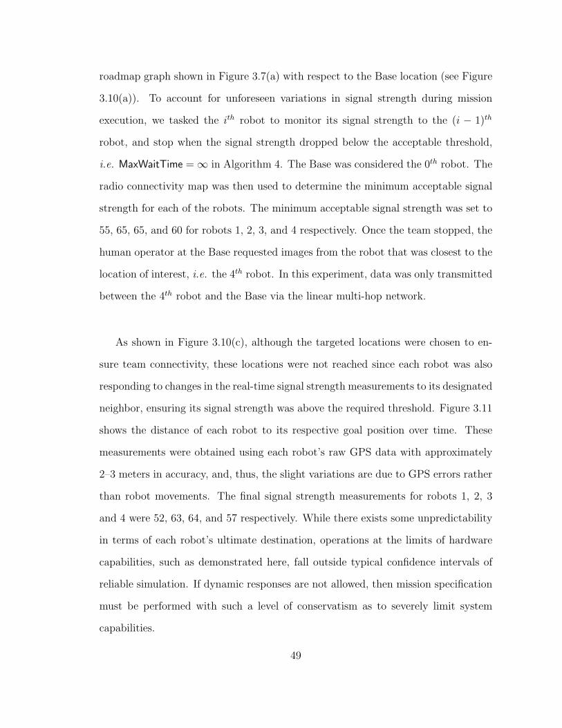
roadmap graph shown in Figure 3.7(a) with respect to the Base location (see Figure

3.10(a)). To account for unforeseen variations in signal strength during mission

execution, we tasked the ith robot to monitor its signal strength to the (i − 1)th

robot, and stop when the signal strength dropped below the acceptable threshold,

i.e. MaxWaitTime =∞ in Algorithm 4. The Base was considered the 0th robot. The

radio connectivity map was then used to determine the minimum acceptable signal

strength for each of the robots. The minimum acceptable signal strength was set to

55, 65, 65, and 60 for robots 1, 2, 3, and 4 respectively. Once the team stopped, the

human operator at the Base requested images from the robot that was closest to the

location of interest, i.e. the 4th robot. In this experiment, data was only transmitted

between the 4th robot and the Base via the linear multi-hop network.

As shown in Figure 3.10(c), although the targeted locations were chosen to en-

sure team connectivity, these locations were not reached since each robot was also

responding to changes in the real-time signal strength measurements to its designated

neighbor, ensuring its signal strength was above the required threshold. Figure 3.11

shows the distance of each robot to its respective goal position over time. These

measurements were obtained using each robot’s raw GPS data with approximately

2–3 meters in accuracy, and, thus, the slight variations are due to GPS errors rather

than robot movements. The final signal strength measurements for robots 1, 2, 3

and 4 were 52, 63, 64, and 57 respectively. While there exists some unpredictability

in terms of each robot’s ultimate destination, operations at the limits of hardware

capabilities, such as demonstrated here, fall outside typical confidence intervals of

reliable simulation. If dynamic responses are not allowed, then mission specification

must be performed with such a level of conservatism as to severely limit system

capabilities.

49

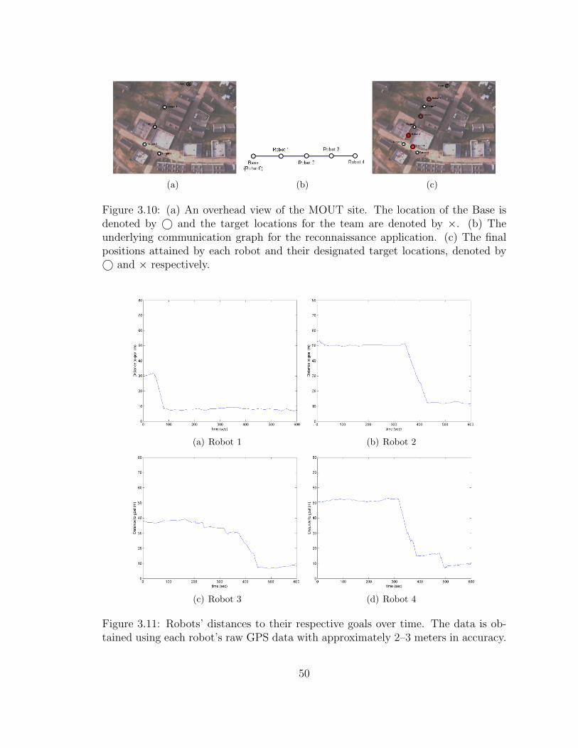
(a) (b) (c)

Figure 3.10: (a) An overhead view of the MOUT site. The location of the Base isdenoted by © and the target locations for the team are denoted by ×. (b) Theunderlying communication graph for the reconnaissance application. (c) The finalpositions attained by each robot and their designated target locations, denoted by© and × respectively.

(a) Robot 1 (b) Robot 2

(c) Robot 3 (d) Robot 4

Figure 3.11: Robots’ distances to their respective goals over time. The data is ob-tained using each robot’s raw GPS data with approximately 2–3 meters in accuracy.

50

Perimeter Surveillance Application

These next experiments were based on a perimeter surveillance application where

robots would navigate to positions on the desired perimenter and send imagery data

back to a base station. In our experiments, we tasked a team of four robots to go

to four separate goal positions where the positions were chosen to represent distinct

locations on the perimeter of interest. In addition, each robot was also tasked to

monitor its signal strength or estimated available bandwidth to the Base while con-

tinuously sending imagery data to it. Thus, every robot was sending approximately

10 KB JPEG images back to the Base, as compared to the previous experiment,

where only one robot was sending data to the Base.

At the Base, a display panel with each robot’s imagery data was provided to the

operator. In the event the display panel did not receive new data from a particular

robot over a specified interval of time, the panel would highlight the display box for

that particular robot. The objective of these experiments was to focus on an indi-

vidual robot’s ability to respond to changes in signal strength or perceived available

bandwidth. Thus, we only considered single hop network connections between each

robot and the Base. Additionally, to avoid robots being caught in a “local mini-

mum” due to dynamic changes in the environment that may affect signal strength

measurements, and to better emphasize the reactive nature of our controllers, we set

the MaxWaitTime in Algorithm 4 to a finite time.

The first such experiment conducted at this location demonstrates the reactive

controller in the presence of dynamic network disturbances. In this experiment, the

network disturbance was caused by the addition of a second robot to a network

originally used by a single robot transmitting a video stream to the Base. As shown

earlier in Figure 1.2, as new members are introduced into the team, the maximum

51

bandwidth available to each robot drops.

Figure 3.13 shows how our controller responded to the addition of the second

robot. We first deployed a single robot, Robot 1, to a goal position and required

that it continuously send imagery data to the Base while maintaining a minimum

transaction rate of 7 transactions per second. This can be seen in the top graph

of Figure 3.13 where each marker denotes the number of transactions received in

between the time of the current marker and the one before it, approximately 10 sec-

onds. The MaxWaitTime variable in Algorithm 4 was set to 30 seconds. A schematic

of the deployment strategy is shown in Figure 3.12. At around t = 60s, Robot 1

settled to a location about halfway to the goal as shown in the bottom graph of

Figure 3.13. Between t = 90s and t = 125s, the robot attempted to reach its goal

a second time and settled to a similar location shown in bottom two graphs in Fig-

ure 3.13. A second robot, Robot 2, transmitting to the Base was introduced to the

network at approximately t = 130s, as shown in the first graph of Figure 3.13. Im-

mediately, Robot 1 was no longer able to maintain the required transaction rate and

therefore began moving back towards the Base in an effort to boost its transaction

rate. This can be seen in the last graph of Figure 3.13 where the robot’s distance to

its goal starts increasing. Put simply, a robot was tasked with sending video back

to a base station as it monitored a perimeter. In the early stages of the mission,

the robot could transmit video at a high rate, but as the robot moved further away

from the base station, the rate at which it could transmit video dropped. The robot

continued moving until the transmission rate hit a pre-defined threshold. At this

point, the robot stabilized its distance from the base station in order to maintain

the minimum required transmission rate. Once another network user was added, the

first robot had to move yet closer to the base station. This response is made because

the transmission rate for a single robot is a function both of total network usage

52

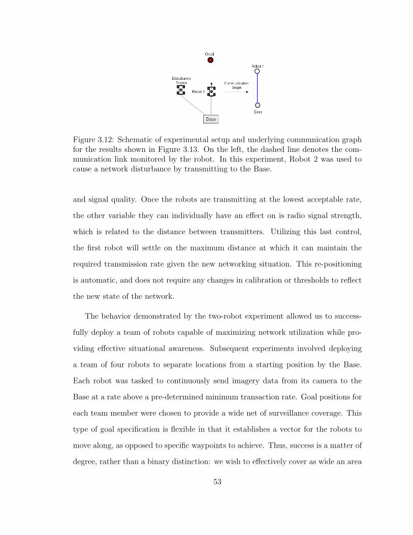
Figure 3.12: Schematic of experimental setup and underlying communication graphfor the results shown in Figure 3.13. On the left, the dashed line denotes the com-munication link monitored by the robot. In this experiment, Robot 2 was used tocause a network disturbance by transmitting to the Base.

and signal quality. Once the robots are transmitting at the lowest acceptable rate,

the other variable they can individually have an effect on is radio signal strength,

which is related to the distance between transmitters. Utilizing this last control,

the first robot will settle on the maximum distance at which it can maintain the

required transmission rate given the new networking situation. This re-positioning

is automatic, and does not require any changes in calibration or thresholds to reflect

the new state of the network.

The behavior demonstrated by the two-robot experiment allowed us to success-

fully deploy a team of robots capable of maximizing network utilization while pro-

viding effective situational awareness. Subsequent experiments involved deploying

a team of four robots to separate locations from a starting position by the Base.

Each robot was tasked to continuously send imagery data from its camera to the

Base at a rate above a pre-determined minimum transaction rate. Goal positions for

each team member were chosen to provide a wide net of surveillance coverage. This

type of goal specification is flexible in that it establishes a vector for the robots to

move along, as opposed to specific waypoints to achieve. Thus, success is a matter of

degree, rather than a binary distinction: we wish to effectively cover as wide an area

53

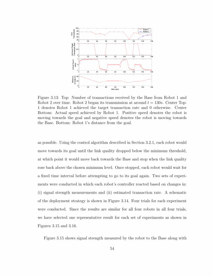
Figure 3.13: Top: Number of transactions received by the Base from Robot 1 andRobot 2 over time. Robot 2 began its transmission at around t = 130s. Center Top:1 denotes Robot 1 achieved the target transaction rate and 0 otherwise. CenterBottom: Actual speed achieved by Robot 1. Positive speed denotes the robot ismoving towards the goal and negative speed denotes the robot is moving towardsthe Base. Bottom: Robot 1’s distance from the goal.

as possible. Using the control algorithm described in Section 3.2.1, each robot would

move towards its goal until the link quality dropped below the minimum threshold,

at which point it would move back towards the Base and stop when the link quality

rose back above the chosen minimum level. Once stopped, each robot would wait for

a fixed time interval before attempting to go to its goal again. Two sets of experi-

ments were conducted in which each robot’s controller reacted based on changes in:

(i) signal strength measurements and (ii) estimated transaction rate. A schematic

of the deployment strategy is shown in Figure 3.14. Four trials for each experiment

were conducted. Since the results are similar for all four robots in all four trials,

we have selected one representative result for each set of experiments as shown in

Figures 3.15 and 3.16.

Figure 3.15 shows signal strength measured by the robot to the Base along with

54

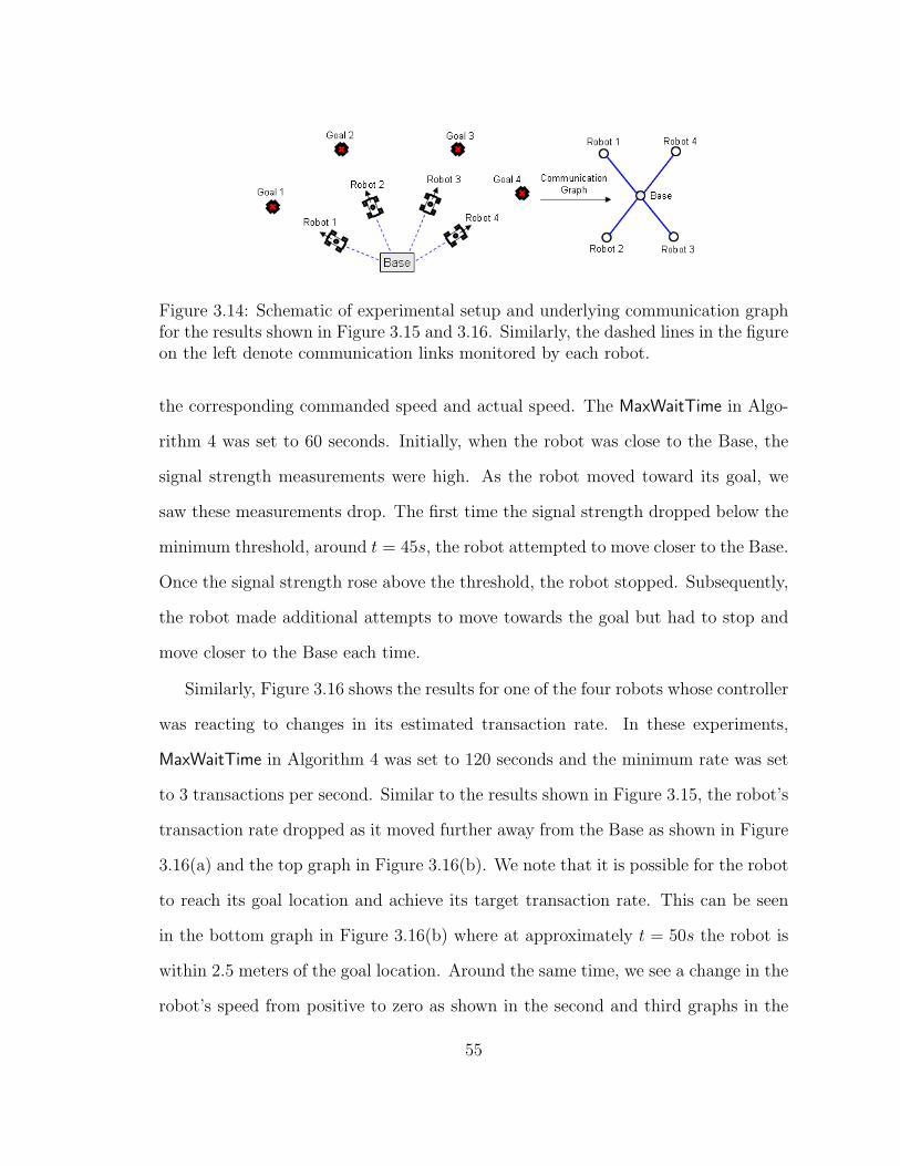
Figure 3.14: Schematic of experimental setup and underlying communication graphfor the results shown in Figure 3.15 and 3.16. Similarly, the dashed lines in the figureon the left denote communication links monitored by each robot.

the corresponding commanded speed and actual speed. The MaxWaitTime in Algo-

rithm 4 was set to 60 seconds. Initially, when the robot was close to the Base, the

signal strength measurements were high. As the robot moved toward its goal, we

saw these measurements drop. The first time the signal strength dropped below the

minimum threshold, around t = 45s, the robot attempted to move closer to the Base.

Once the signal strength rose above the threshold, the robot stopped. Subsequently,

the robot made additional attempts to move towards the goal but had to stop and

move closer to the Base each time.

Similarly, Figure 3.16 shows the results for one of the four robots whose controller

was reacting to changes in its estimated transaction rate. In these experiments,

MaxWaitTime in Algorithm 4 was set to 120 seconds and the minimum rate was set

to 3 transactions per second. Similar to the results shown in Figure 3.15, the robot’s

transaction rate dropped as it moved further away from the Base as shown in Figure

3.16(a) and the top graph in Figure 3.16(b). We note that it is possible for the robot

to reach its goal location and achieve its target transaction rate. This can be seen

in the bottom graph in Figure 3.16(b) where at approximately t = 50s the robot is

within 2.5 meters of the goal location. Around the same time, we see a change in the

robot’s speed from positive to zero as shown in the second and third graphs in the

55

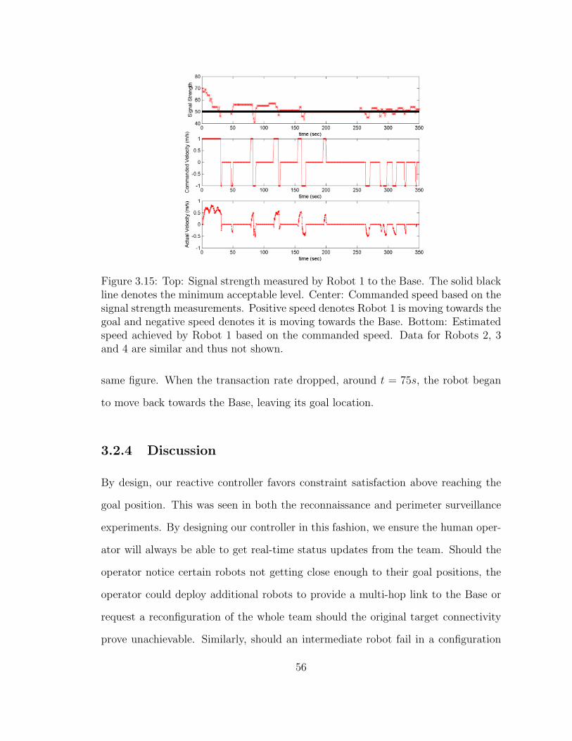
Figure 3.15: Top: Signal strength measured by Robot 1 to the Base. The solid blackline denotes the minimum acceptable level. Center: Commanded speed based on thesignal strength measurements. Positive speed denotes Robot 1 is moving towards thegoal and negative speed denotes it is moving towards the Base. Bottom: Estimatedspeed achieved by Robot 1 based on the commanded speed. Data for Robots 2, 3and 4 are similar and thus not shown.

same figure. When the transaction rate dropped, around t = 75s, the robot began

to move back towards the Base, leaving its goal location.

3.2.4 Discussion

By design, our reactive controller favors constraint satisfaction above reaching the

goal position. This was seen in both the reconnaissance and perimeter surveillance

experiments. By designing our controller in this fashion, we ensure the human oper-

ator will always be able to get real-time status updates from the team. Should the

operator notice certain robots not getting close enough to their goal positions, the

operator could deploy additional robots to provide a multi-hop link to the Base or

request a reconfiguration of the whole team should the original target connectivity

prove unachievable. Similarly, should an intermediate robot fail in a configuration

56

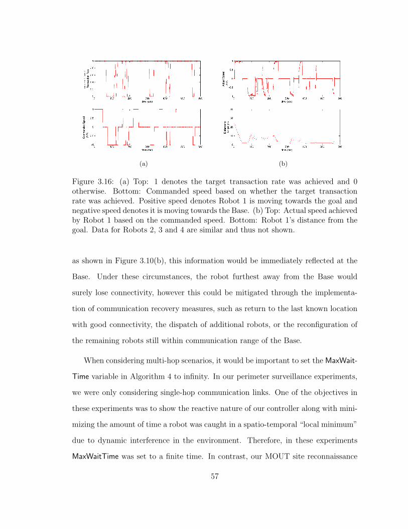
(a) (b)

Figure 3.16: (a) Top: 1 denotes the target transaction rate was achieved and 0otherwise. Bottom: Commanded speed based on whether the target transactionrate was achieved. Positive speed denotes Robot 1 is moving towards the goal andnegative speed denotes it is moving towards the Base. (b) Top: Actual speed achievedby Robot 1 based on the commanded speed. Bottom: Robot 1’s distance from thegoal. Data for Robots 2, 3 and 4 are similar and thus not shown.

as shown in Figure 3.10(b), this information would be immediately reflected at the

Base. Under these circumstances, the robot furthest away from the Base would

surely lose connectivity, however this could be mitigated through the implementa-

tion of communication recovery measures, such as return to the last known location

with good connectivity, the dispatch of additional robots, or the reconfiguration of

the remaining robots still within communication range of the Base.

When considering multi-hop scenarios, it would be important to set the MaxWait-

Time variable in Algorithm 4 to infinity. In our perimeter surveillance experiments,

we were only considering single-hop communication links. One of the objectives in

these experiments was to show the reactive nature of our controller along with mini-

mizing the amount of time a robot was caught in a spatio-temporal “local minimum”

due to dynamic interference in the environment. Therefore, in these experiments

MaxWaitTime was set to a finite time. In contrast, our MOUT site reconnaissance

57

experiment, where the objective was to deploy a multi-hop network, did not have

these recovery responses because we did not want the constant back and forth motion

to affect the robots ability to send data through the multi-hop network. Had the

reactive response been present, it is very likely the constant back and forth motion

would affect the team’s ability to reliably relay information to the Base.

In all our experiments, the minimum thresholds were chosen based on a com-

bination of previously collected data and/or specific mission requirements. In the

reconnaissance experiment, signal strength thresholds were determined based on

information gleaned from a radio connectivity map. On the other hand, when con-

sidering perceived network bandwidth, the minimum acceptable threshold was de-

termined based on hardware limitations in conjunction with acceptable transmission

rates based on mission requirements specified by the human operator.

Lastly, our reactive controllers can be easily decentralized based on the method-

ology proposed in [40], and thus scaled to large number of robots. Rather than

specifying specific goal positions for every robot in the team, [40] specifies a one-

dimensional boundary curve for the team. This, however, does not necessarily mean

the existing network would be able to handle the increase in traffic brought on by

the increase in team size.

3.3 Conclusion

In this chapter, we have presented a paradigm and algorithms for deploying a mobile

robot network with specifications on end-to-end performance. Our approach entails

the automated construction of a radio map for a partially known urban environment

which can then be used to deploy a team of robots, and control algorithms that drive

the team to designated targets on some desired boundary (curve) while maintaining

58

communication link quality.

There are two main contributions. First, we developed a method for obtain-

ing radio signal strength maps that can be used to plan multi-robot tasks and also

serve as useful perceptual information. Second, since a radio signal strength map

only serves to create a nominal model, we have shown the importance for individ-

ual robots to have the ability to monitor communication links, in particular signal

strength measurements as well as available data throughput. This method of link

quality control provides scalability in the number of robots that may be added to the

network, and an abstraction of the underlying network architecture. Since the robots

constantly strive to maximize network usage efficiency, robots may be added to, or

removed from the network without changes to any thresholds or calibration numbers.

This type of deployment characteristic is extremely important as robot team sizes

scale, as we want teams to take advantage of bandwidth when it is available, and

automatically scale back individual usage as available resources are stretched thin.

Moreover, we have also shown that channel contention between multiple nodes can

have a severe adverse effect on total network throughput. By monitoring successful

transactions, we give our robots the ability to throttle their own network usage such

that the transmission rates of each robot stabilize to levels that make efficient use of

the network.

Additionally, as shown in our perimeter surveillance experiments, in dynamic

environments where radio propagation characteristics may exhibit significant changes

over time, it is good practice for agents to always attempt to move closer to the goal

regardless of where they first come to a stop. The forward movement is the only

way to confirm that positions closer to the goal violate communication constraints,

and to ensure the agents always minimize their distance to the goal location while

remaining connected. Ideally, robotic agents should be deployed with the capability

59

of monitoring inter-agent signal strengths as well as data throughput. In general,

signal strength is a good indicator of potential connectivity while data throughput

can efficiently be used to ensure minimum actual data throughput rates. Combining

the two, good signal strength paired with unacceptably low throughput may indicate

a need for human attention to the network architecture and the demands being placed

on it. As such, the communication medium becomes a useful sensor that can be used

to monitor the effectiveness of any given multi-robot deployment.

Reactive navigation controllers such as the one presented provide a reliable foun-

dation on which to build scalable, portable, high-level tasks. The reactive controller

acts as a scenario-independent support that allows for the deployment of a robot

team to any location, regardless of prior reconnaissance. As shown in our reconnais-

sance experiment, behaviors built on such a controller inherit respect for network

constraints, thereby allowing both flexible goal specification and more deliberative

trajectory planning done with environmental models that do not necessarily capture

all static and dynamic aspects of an environment’s radio propagation characteris-

tics. Since the team always remain connected during mission execution, potential

failure points in the communication network, as perceived by individual robots, can

be relayed back to the base station to trigger contingency management routines, e.g.

deployment of additional robots or a reallocation of resources. While the strategies

presented in this work assign the highest priority to maintaining the network, appli-

cations that may benefit from a relaxation of this constraint provide a direction for

future work.

60

Chapter 4

Scalable Motion Control Strategies

for Robotic Swarms with Obstacle

Avoidance

As the size of robot teams increases, there has been a shift towards a swarming

paradigm where robots are programmed with simple but identical behaviors that

can be realized with limited on-board computational, communication and sensing

resources. Such swarming behaviors are often seen in nature, specifically in biolog-

ical systems composed of large number of organisms which individually lack either

the communication or computational capabilities required for centralized control.

Examples of such behaviors can be seen in the group dynamics of beehives [13], ant

colonies [74], bird flocks, steer herds and fish schools [66].

We are interested in deploying robotic teams for applications such as perime-

ter surveillance, monitoring of specified areas, and cooperative manipulation where

robots may need to surround an object to transport it from one location to another.

In these situations, robots may have to communicate with each other in order to

61

integrate and fuse the information acquired by various sensors and as such, limited

bandwidth must be preserved to enable the communication of crucial data between

team members and/or to a base station. This is especially critical when we con-

sider very large teams where bandwidth often becomes the limiting factor in agents’

abilities to transmit data. In these situations, robots must have the ability to ac-

complish the necessary tasks while minimizing communication overhead and operate

with little to no human supervision.

This work addresses the synthesis of decentralized controllers that guarantee the

stability and convergence of all the robots to the boundary of a specified shape

such that each robot has non-zero velocity tangential to the desired boundary. We

present a communicationless strategy where collision avoidance is achieved via a

prioritization schemed based on each robot’s relation to its immediate neighbors.

While part of our approach is similar in spirit to the gyroscopic forces proposed by

Chang and Marsden [18], we achieve collision and obstacle avoidance by modulating

each robot’s speeds independently using smooth positive scalar functions. Thus,

unlike Chang and Marsden, neighbors with higher priorities result in slowing down

a robot’s travel speed rather than exerting a gyroscopic force on the agent. While

we assume that agents are holonomic, it is possible to extend our methodology to

include non–holonomic robots. This can be achieved because we consider disk–

shaped robots, thus enabling the use of feedback linearization techniques to linearize

the non–holonomic model away from each robot’s center of rotation.

We begin with the problem formulation and provide some background to our

approach in Section 4.1. The controller synthesis is described in Section 4.2. The

safety, stability and convergence properties of the controller are discussed in Section

4.3 with simulation results presented in Section 4.4. Lastly, we provide an exten-

sion of our proposed controller to handle obstacles in close proximity to the desired

62

boundary in Section 4.5 and conclude with a discussion on directions for future work

in Section 4.6.

4.1 Problem Formulation

We consider a group of N planar, fully actuated robots each with kinematics given

by

qi = ui (4.1)

where qi = (xi, yi)T and ui denote the ith agent’s position and control input. Thus,

the robot state is a 2× 1 state vector and the state of the team of robots is given by

q =[qT1 . . . q

TN

]T ∈ Q ⊂ R2N . We assume disk-shaped agents, each with finite radius

ri.

We would like to design control inputs that will stabilize the group of N robots to

the boundary (curve) of a desired smooth, compact set, e.g. shape. We would like to

achieve this such that agents have non-zero velocities tangent to the boundary curve,

enabling them to travel along the boundary curve in a counter-clockwise direction,

all the while avoiding collisions with one another. This is relevant for applications

such as perimeter surveillance, surrounding objects for capture, or cordoning off and

containing hazardous regions after chemical spills or biological attacks.

We assume the workspace, W , is described by the set,

W = q| ‖q‖ ≤ R0,

and let ∂W denote the boundary of the workspace. For a desired smooth star shape

set, S, we denote ∂S to be the boundary of S and, similar to [40], we assume that ∂S

is described by a smooth, regular, simple, closed curve of the form s(x, y)− s0 = 0.

63

Furthermore, we assume the agents have the capability to localize themselves in some

global coordinate frame and the ability to sense the proximity of their teammates

and/or obstacles within the environment. As such, we define the neighborhood of qi

by the range and field of view of the sensing hardware and denote the set of neighbors

in this region by Γi. For collision avoidance purposes, we assume a circular influence

range, Ri, such that collision/obstacle avoidance maneuvers are active when agents

are within each other’s influence range.

The objective is to construct artificial potential functions, ϕ, for the obstacle free

environment and augment these with additional behaviors that can locally modify the

feedback policy derived from ϕ to enable the team of N agents to: 1) stabilize onto

the desired closed curve (orbit) with non-zero velocities in the orbit’s tangent space;

2) avoid collisions with other agents; and 3) avoid collision with unmodeled robot–

sized obstacles in the environment. We outline our methodology in the following

section.

4.2 Methodology

4.2.1 Assumptions

Given a smooth star shape S, a team of N robots each with radius ri > 0 and

influence range Ri > 0, we define r = maxri ∀ i ri and R = maxRi ∀ iRi. Our goal is to

synthesize decentralized controllers that will allow a team to converge to the desired

orbit with non-zero velocities in the orbit’s tanget space while avoiding collisions.

Therefore, the length of ∂S, L, naturally imposes an upper bound on the number of

robots, e.g. Nmax > 0, that can travel along the boundary with non-zero velocity.

Thus, we make the following assumptions:

64

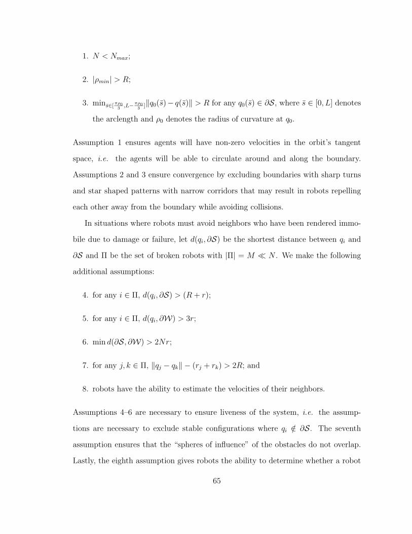
1. N < Nmax;

2. |ρmin| > R;

3. mins∈[πρ03,L−πρ0

3]‖q0(s)− q(s)‖ > R for any q0(s) ∈ ∂S, where s ∈ [0, L] denotes

the arclength and ρ0 denotes the radius of curvature at q0.

Assumption 1 ensures agents will have non-zero velocities in the orbit’s tangent

space, i.e. the agents will be able to circulate around and along the boundary.

Assumptions 2 and 3 ensure convergence by excluding boundaries with sharp turns

and star shaped patterns with narrow corridors that may result in robots repelling

each other away from the boundary while avoiding collisions.

In situations where robots must avoid neighbors who have been rendered immo-

bile due to damage or failure, let d(qi, ∂S) be the shortest distance between qi and

∂S and Π be the set of broken robots with |Π| = M N . We make the following

additional assumptions:

4. for any i ∈ Π, d(qi, ∂S) > (R + r);

5. for any i ∈ Π, d(qi, ∂W) > 3r;

6. min d(∂S, ∂W) > 2Nr;

7. for any j, k ∈ Π, ‖qj − qk‖ − (rj + rk) > 2R; and

8. robots have the ability to estimate the velocities of their neighbors.

Assumptions 4–6 are necessary to ensure liveness of the system, i.e. the assump-

tions are necessary to exclude stable configurations where qi /∈ ∂S. The seventh

assumption ensures that the “spheres of influence” of the obstacles do not overlap.

Lastly, the eighth assumption gives robots the ability to determine whether a robot

65

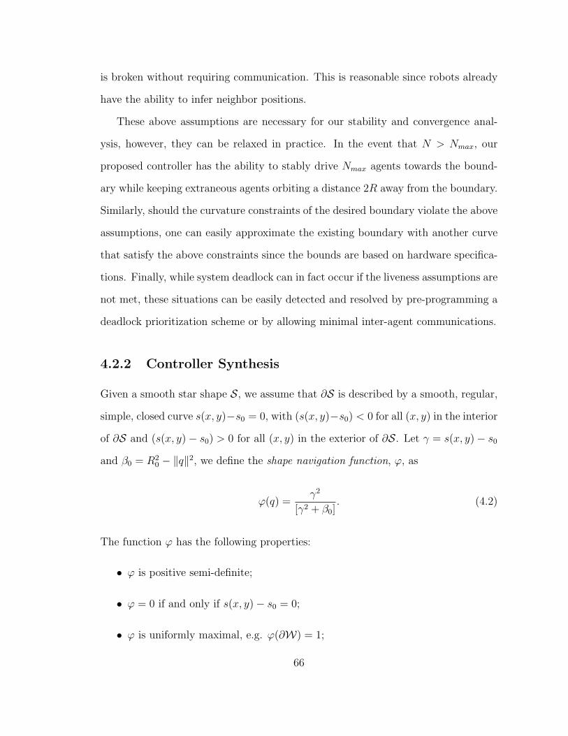
is broken without requiring communication. This is reasonable since robots already

have the ability to infer neighbor positions.

These above assumptions are necessary for our stability and convergence anal-

ysis, however, they can be relaxed in practice. In the event that N > Nmax, our

proposed controller has the ability to stably drive Nmax agents towards the bound-

ary while keeping extraneous agents orbiting a distance 2R away from the boundary.

Similarly, should the curvature constraints of the desired boundary violate the above

assumptions, one can easily approximate the existing boundary with another curve

that satisfy the above constraints since the bounds are based on hardware specifica-

tions. Finally, while system deadlock can in fact occur if the liveness assumptions are

not met, these situations can be easily detected and resolved by pre-programming a

deadlock prioritization scheme or by allowing minimal inter-agent communications.

4.2.2 Controller Synthesis

Given a smooth star shape S, we assume that ∂S is described by a smooth, regular,

simple, closed curve s(x, y)−s0 = 0, with (s(x, y)−s0) < 0 for all (x, y) in the interior

of ∂S and (s(x, y)− s0) > 0 for all (x, y) in the exterior of ∂S. Let γ = s(x, y)− s0

and β0 = R20 − ‖q‖2, we define the shape navigation function, ϕ, as

ϕ(q) =γ2

[γ2 + β0]. (4.2)

The function ϕ has the following properties:

• ϕ is positive semi-definite;

• ϕ = 0 if and only if s(x, y)− s0 = 0;

• ϕ is uniformly maximal, e.g. ϕ(∂W) = 1;

66

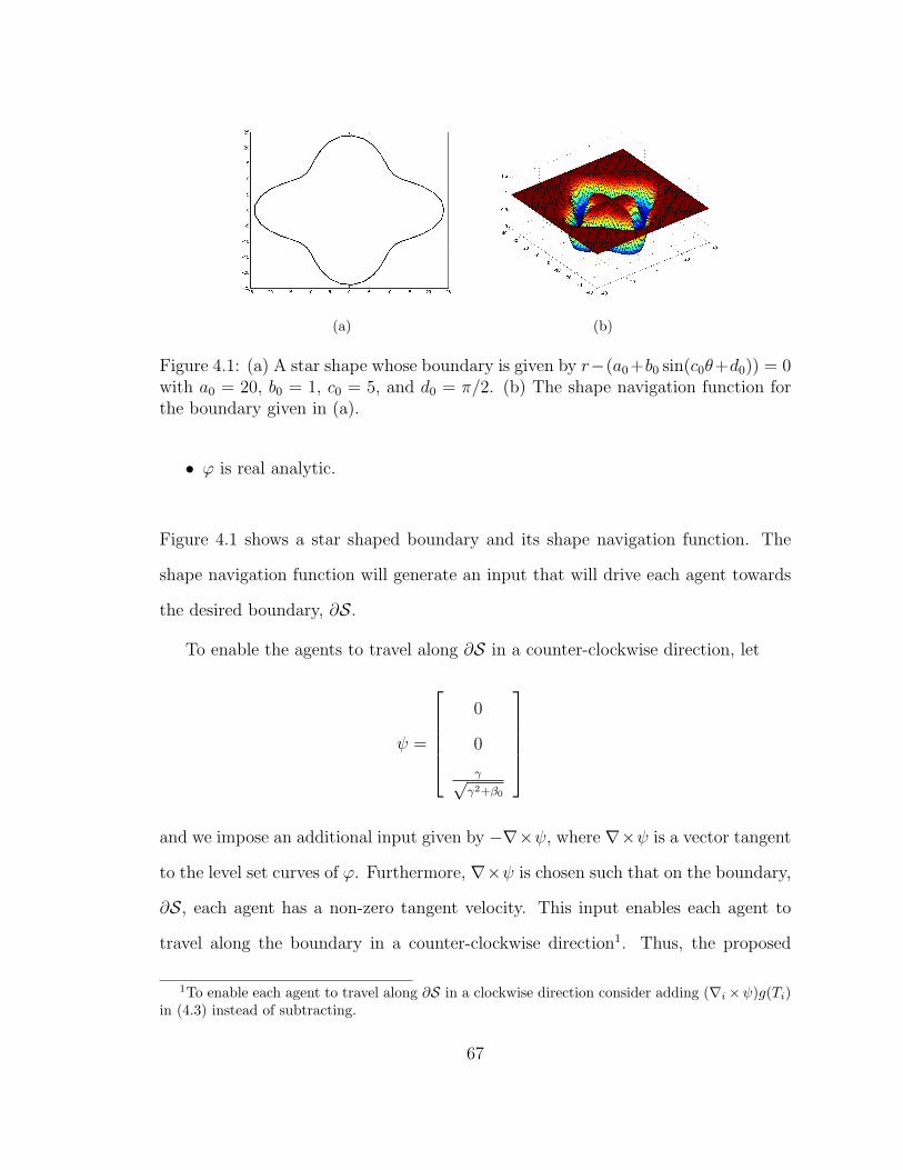
(a) (b)

Figure 4.1: (a) A star shape whose boundary is given by r−(a0 +b0 sin(c0θ+d0)) = 0with a0 = 20, b0 = 1, c0 = 5, and d0 = π/2. (b) The shape navigation function forthe boundary given in (a).

• ϕ is real analytic.

Figure 4.1 shows a star shaped boundary and its shape navigation function. The

shape navigation function will generate an input that will drive each agent towards

the desired boundary, ∂S.

To enable the agents to travel along ∂S in a counter-clockwise direction, let

ψ =

0

0

γ√γ2+β0

and we impose an additional input given by −∇×ψ, where ∇×ψ is a vector tangent

to the level set curves of ϕ. Furthermore, ∇×ψ is chosen such that on the boundary,

∂S, each agent has a non-zero tangent velocity. This input enables each agent to

travel along the boundary in a counter-clockwise direction1. Thus, the proposed

1To enable each agent to travel along ∂S in a clockwise direction consider adding (∇i×ψ)g(Ti)in (4.3) instead of subtracting.

67

(a) (b) (c)

Figure 4.2: Vector fields for the star shaped boundary given by r− (a0 + b0 sin(c0θ+d0)) = 0 with a0 = 20, b0 = 1, c0 = 5, and d0 = π/2. (a) Vector field given by−∇ϕ. (b) Vector field given by −∇ × ψ. (c) Vector field given by equation (4.3)with f(Ni) = 1 and g(Ti) = 1.

decentralized controller in an environment with no obstacles is given by:

ui = −∇iϕi · f(Ni)−∇i × ψi · g(Ti) (4.3)

where ∇i denotes differentiation with respect to agent i’s coordinates and ϕi = ϕ(qi)

and ψi = ψ(qi). The functions f(Ni) and g(Ti) are positive scalar functions used

to modulate each agent’s velocity for collision avoidance and their construction is

described in the following section. The first term of (4.3) drives the agents towards

∂S and the second term drives the agents along the level set curves of ϕ in a counter-

clockwise direction. Figures 4.2(a) and 4.2(b) show the vector fields generated by the

first and second terms of Equation (4.3) for a star-shaped boundary. Figure 4.2(c)

shows the combined vector fields for the same boundary with f(Ni) = g(Ti) = 1. In

the remainder of this paper we will refer to the first and second term of (4.3) as the

descent and tangential velocities of agent i.

68

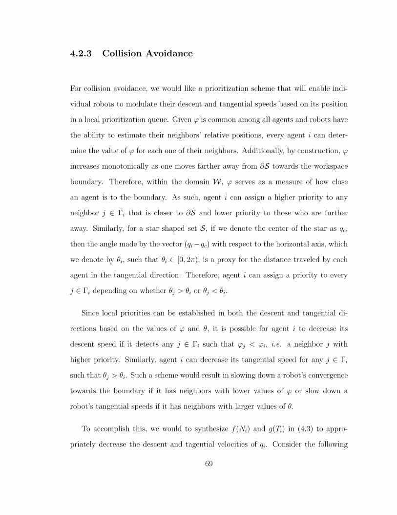
4.2.3 Collision Avoidance

For collision avoidance, we would like a prioritization scheme that will enable indi-

vidual robots to modulate their descent and tangential speeds based on its position

in a local prioritization queue. Given ϕ is common among all agents and robots have

the ability to estimate their neighbors’ relative positions, every agent i can deter-

mine the value of ϕ for each one of their neighbors. Additionally, by construction, ϕ

increases monotonically as one moves farther away from ∂S towards the workspace

boundary. Therefore, within the domain W , ϕ serves as a measure of how close

an agent is to the boundary. As such, agent i can assign a higher priority to any

neighbor j ∈ Γi that is closer to ∂S and lower priority to those who are further

away. Similarly, for a star shaped set S, if we denote the center of the star as qc,

then the angle made by the vector (qi−qc) with respect to the horizontal axis, which

we denote by θi, such that θi ∈ [0, 2π), is a proxy for the distance traveled by each

agent in the tangential direction. Therefore, agent i can assign a priority to every

j ∈ Γi depending on whether θj > θi or θj < θi.

Since local priorities can be established in both the descent and tangential di-

rections based on the values of ϕ and θ, it is possible for agent i to decrease its

descent speed if it detects any j ∈ Γi such that ϕj < ϕi, i.e. a neighbor j with

higher priority. Similarly, agent i can decrease its tangential speed for any j ∈ Γi

such that θj > θi. Such a scheme would result in slowing down a robot’s convergence

towards the boundary if it has neighbors with lower values of ϕ or slow down a

robot’s tangential speeds if it has neighbors with larger values of θ.

To accomplish this, we would to synthesize f(Ni) and g(Ti) in (4.3) to appro-

priately decrease the descent and tagential velocities of qi. Consider the following

69

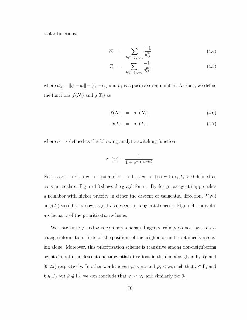
scalar functions:

Ni =∑

j∈Γi,ϕj<ϕi

−1

dp1ij(4.4)

Ti =∑

j∈Γi,θj>θi

−1

dp1ij, (4.5)

where dij = ‖qi− qj‖− (ri + rj) and p1 is a positive even number. As such, we define

the functions f(Ni) and g(Ti) as

f(Ni) = σ−(Ni), (4.6)

g(Ti) = σ−(Ti), (4.7)

where σ− is defined as the following analytic switching function:

σ−(w) =1

1 + e−t1(w−t2).

Note as σ− → 0 as w → −∞ and σ− → 1 as w → +∞ with t1, t2 > 0 defined as

constant scalars. Figure 4.3 shows the graph for σ−. By design, as agent i approaches

a neighbor with higher priority in either the descent or tangential direction, f(Ni)

or g(Ti) would slow down agent i’s descent or tangential speeds. Figure 4.4 provides

a schematic of the prioritization scheme.

We note since ϕ and ψ is common among all agents, robots do not have to ex-

change information. Instead, the positions of the neighbors can be obtained via sens-

ing alone. Moreover, this prioritization scheme is transitive among non-neighboring

agents in both the descent and tangential directions in the domains given by W and

[0, 2π) respectively. In other words, given ϕi < ϕj and ϕj < ϕk such that i ∈ Γj and

k ∈ Γj but k /∈ Γi, we can conclude that ϕi < ϕk and similarly for θi.

70

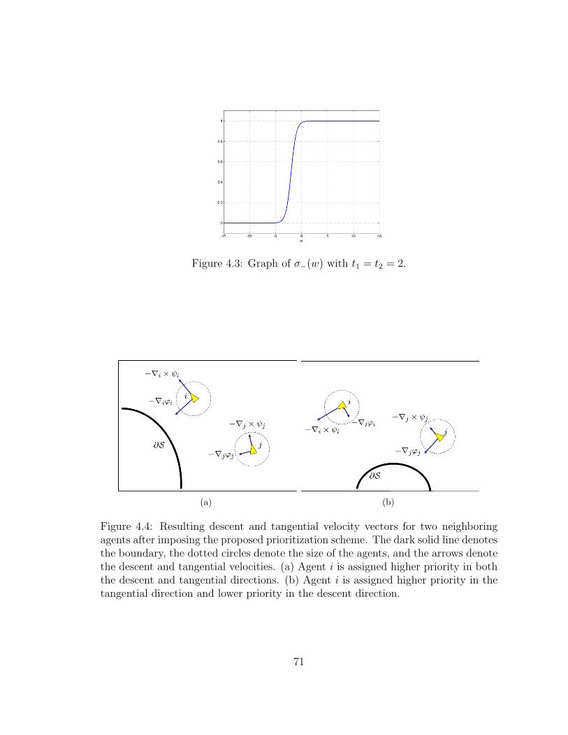
Figure 4.3: Graph of σ−(w) with t1 = t2 = 2.

(a) (b)

Figure 4.4: Resulting descent and tangential velocity vectors for two neighboringagents after imposing the proposed prioritization scheme. The dark solid line denotesthe boundary, the dotted circles denote the size of the agents, and the arrows denotethe descent and tangential velocities. (a) Agent i is assigned higher priority in boththe descent and tangential directions. (b) Agent i is assigned higher priority in thetangential direction and lower priority in the descent direction.

71

4.2.4 Obstacle Avoidance

While the proposed collision avoidance scheme ensures inter-agent collisions do not

occur, this is only guaranteed while all agents have non-zero velocities. Should an

agent fail and become immobilized, the existing methodology may result in prevent-

ing the remainder of the team to converge to the desired boundary and resulting in

a potential deadlock situation.

In this section, we extend the decentralized controller described in the previous

section to give active robots the ability to avoid circular obstacles that are compa-

rable, in size, to other robots, thus avoiding collisions with robots that have been

rendered immobile for one reason or another. This will ensure graceful degradation

of our system in the event of robot failures and gives the agents the ability to avoid

unmodeled obstacles.

Consider the following decentralized controller:

ui = −∇iϕi · f(Ni)−∇i × ψi · g(Ti)−∑

j∈Γi,‖vj‖=0

∇i × βjdp2ij

h(qi, qj) (4.8)

with 0 < p2 < p1, and βj and h(qi, qj) respectively defined as:

βj =

0

0

dij√d2ij+β0

,

h(qi, qj) =(f(Ni)σ−(ϕij)− f(Ni)σ+(θij)σ+(ϕij)

).

72

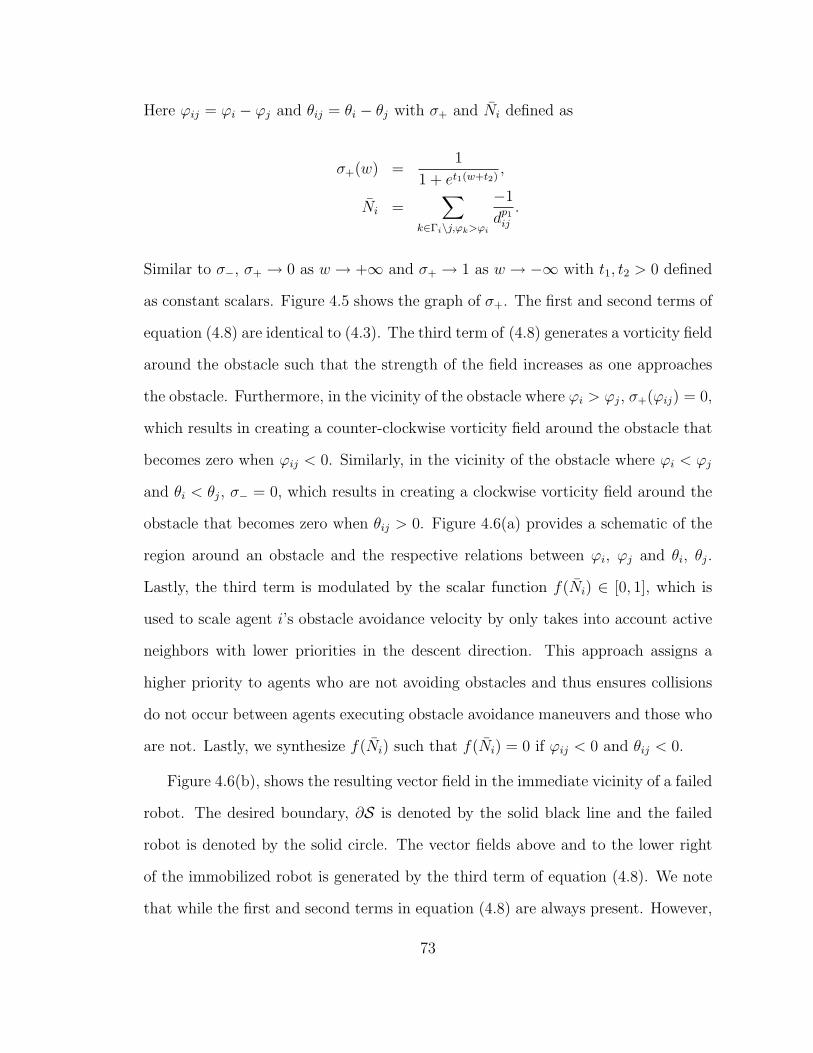
Here ϕij = ϕi − ϕj and θij = θi − θj with σ+ and Ni defined as

σ+(w) =1

1 + et1(w+t2),

Ni =∑

k∈Γi\j,ϕk>ϕi

−1

dp1ij.

Similar to σ−, σ+ → 0 as w → +∞ and σ+ → 1 as w → −∞ with t1, t2 > 0 defined

as constant scalars. Figure 4.5 shows the graph of σ+. The first and second terms of

equation (4.8) are identical to (4.3). The third term of (4.8) generates a vorticity field

around the obstacle such that the strength of the field increases as one approaches

the obstacle. Furthermore, in the vicinity of the obstacle where ϕi > ϕj, σ+(ϕij) = 0,

which results in creating a counter-clockwise vorticity field around the obstacle that

becomes zero when ϕij < 0. Similarly, in the vicinity of the obstacle where ϕi < ϕj

and θi < θj, σ− = 0, which results in creating a clockwise vorticity field around the

obstacle that becomes zero when θij > 0. Figure 4.6(a) provides a schematic of the

region around an obstacle and the respective relations between ϕi, ϕj and θi, θj.

Lastly, the third term is modulated by the scalar function f(Ni) ∈ [0, 1], which is

used to scale agent i’s obstacle avoidance velocity by only takes into account active

neighbors with lower priorities in the descent direction. This approach assigns a

higher priority to agents who are not avoiding obstacles and thus ensures collisions

do not occur between agents executing obstacle avoidance maneuvers and those who

are not. Lastly, we synthesize f(Ni) such that f(Ni) = 0 if ϕij < 0 and θij < 0.

Figure 4.6(b), shows the resulting vector field in the immediate vicinity of a failed

robot. The desired boundary, ∂S is denoted by the solid black line and the failed

robot is denoted by the solid circle. The vector fields above and to the lower right

of the immobilized robot is generated by the third term of equation (4.8). We note

that while the first and second terms in equation (4.8) are always present. However,

73

Figure 4.5: Graph of σ+(w) with t1 = t2 = 2.

by construction, f(·) and g(·) tend to zero as a robot approaches the immobilized

agent.

4.3 Safety and Stability Results

In this section, we first consider the stability and covergence properties of the con-

troller given by (4.8) for a group of N robots each with kinematics given by (4.1).

Our first proposition concerns the safety of the system, e.g. no collisions can

occur in finite time, and non-penetration between any two agents.

Proposition 4.3.1 Given ∂S, the system of N robots with kinematics (4.1), the

feedback control law (4.8) satifies (qi − qj)T (vi − vj) > 0 for all i,j pairs as dij → 0.

Proof: For any i and j, we begin with the scenario where i ∈ Γj and j ∈ Γi

and there are no immobiled neighbors in Γi and Γj. Thus, the third term of (4.8) is

74

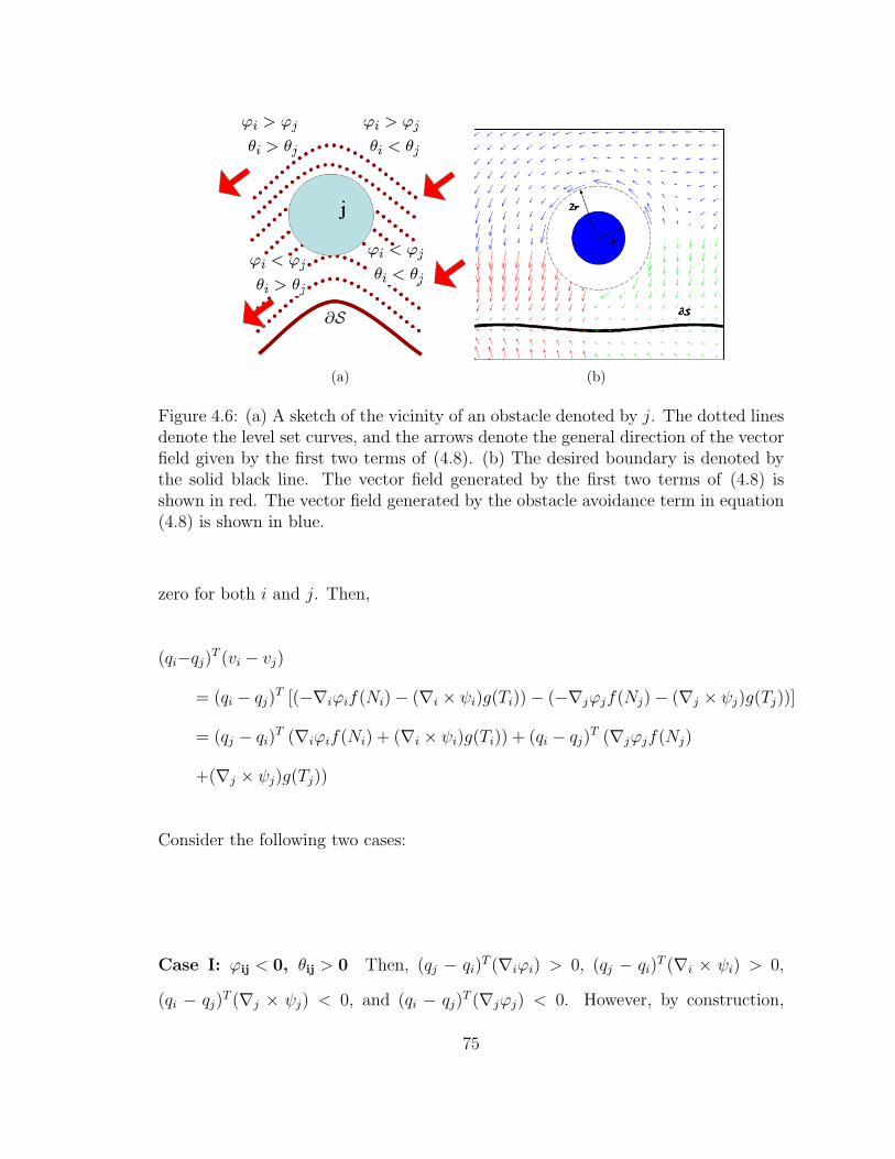
(a) (b)

Figure 4.6: (a) A sketch of the vicinity of an obstacle denoted by j. The dotted linesdenote the level set curves, and the arrows denote the general direction of the vectorfield given by the first two terms of (4.8). (b) The desired boundary is denoted bythe solid black line. The vector field generated by the first two terms of (4.8) isshown in red. The vector field generated by the obstacle avoidance term in equation(4.8) is shown in blue.

zero for both i and j. Then,

(qi−qj)T (vi − vj)

= (qi − qj)T [(−∇iϕif(Ni)− (∇i × ψi)g(Ti))− (−∇jϕjf(Nj)− (∇j × ψj)g(Tj))]

= (qj − qi)T (∇iϕif(Ni) + (∇i × ψi)g(Ti)) + (qi − qj)T (∇jϕjf(Nj)

+(∇j × ψj)g(Tj))

Consider the following two cases:

Case I: ϕij < 0, θij > 0 Then, (qj − qi)T (∇iϕi) > 0, (qj − qi)

T (∇i × ψi) > 0,

(qi − qj)T (∇j × ψj) < 0, and (qi − qj)

T (∇jϕj) < 0. However, by construction,

75

f(Ni) > f(Nj) and g(Ti) > g(Tj). Furthermore, as dij → 0, f(Nj), g(Ti)→ 0. Thus,

(qi − qj)T (vi − vj) = (qj − qi)T (∇iϕif(Ni) + (∇i × ψi)g(Ti)) > 0.

The same analysis holds when ϕij > 0 and θij < 0 by simply interchanging i and j.

Case II: ϕij < 0, θij < 0 This results in (qj−qi)T (∇iϕi) > 0, (qj−qi)T (∇i×ψi) < 0,

(qi − qj)T (∇jϕj) < 0, (qi − qj)

T (∇j × ψj) > 0. By construction, f(Nj) > f(Ni),

g(Ti) < g(Tj), thus as dij → 0, f(Nj), g(Ti)→ 0, with

(qi − qj)T (vi − vj) = (qj − qi)T (∇iϕif(Ni)) + (qi − qj)T (∇j × ψjg(Tj)) > 0.

The same analysis holds when ϕij > 0 and θij > 0 by simply interchanging i and j.

Next, consider the scenario where i ∈ Γj and j ∈ Γi, but j is immobilized, i.e.

‖vj‖ = 0. Then, as dij → 0, f(Ni), g(Ti)→ 0, resulting in

(qi − qj)T (vi − vj) = (qi − qj)T−∇i × βj

dp2ijh(qi, qj)

Regardless of whether ϕi > ϕj or vice versa, by construction (qi − qj) is always

perpendicular to ∇i× βj. Thus, (qi− qj)T (vi− vj) = 0 when i is actively avoiding j.

Once i has successfully avoided j, then (qi− qj)T (vi− vj) > 0 since i will be moving

away from j. This can be seen by setting vj and following the analysis for Case II if

ϕij > 0 or the analysis for Case I if ϕij < 0.

Our next scenario is when i ∈ Γj and j ∈ Γi and there exist a k ∈ Γi but k /∈ Γj

76

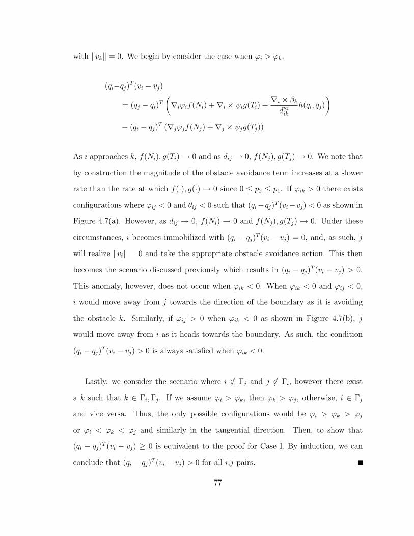
with ‖vk‖ = 0. We begin by consider the case when ϕi > ϕk.

(qi−qj)T (vi − vj)

= (qj − qi)T(∇iϕif(Ni) +∇i × ψig(Ti) +

∇i × βkdp2ik

h(qi, qj)

)− (qi − qj)T (∇jϕjf(Nj) +∇j × ψjg(Tj))

As i approaches k, f(Ni), g(Ti)→ 0 and as dij → 0, f(Nj), g(Tj)→ 0. We note that

by construction the magnitude of the obstacle avoidance term increases at a slower

rate than the rate at which f(·), g(·) → 0 since 0 ≤ p2 ≤ p1. If ϕik > 0 there exists

configurations where ϕij < 0 and θij < 0 such that (qi−qj)T (vi−vj) < 0 as shown in

Figure 4.7(a). However, as dij → 0, f(Ni) → 0 and f(Nj), g(Tj) → 0. Under these

circumstances, i becomes immobilized with (qi − qj)T (vi − vj) = 0, and, as such, j

will realize ‖vi‖ = 0 and take the appropriate obstacle avoidance action. This then

becomes the scenario discussed previously which results in (qi − qj)T (vi − vj) > 0.

This anomaly, however, does not occur when ϕik < 0. When ϕik < 0 and ϕij < 0,

i would move away from j towards the direction of the boundary as it is avoiding

the obstacle k. Similarly, if ϕij > 0 when ϕik < 0 as shown in Figure 4.7(b), j

would move away from i as it heads towards the boundary. As such, the condition

(qi − qj)T (vi − vj) > 0 is always satisfied when ϕik < 0.

Lastly, we consider the scenario where i /∈ Γj and j /∈ Γi, however there exist

a k such that k ∈ Γi,Γj. If we assume ϕi > ϕk, then ϕk > ϕj, otherwise, i ∈ Γj

and vice versa. Thus, the only possible configurations would be ϕi > ϕk > ϕj

or ϕi < ϕk < ϕj and similarly in the tangential direction. Then, to show that

(qi − qj)T (vi − vj) ≥ 0 is equivalent to the proof for Case I. By induction, we can

conclude that (qi − qj)T (vi − vj) > 0 for all i,j pairs.

77

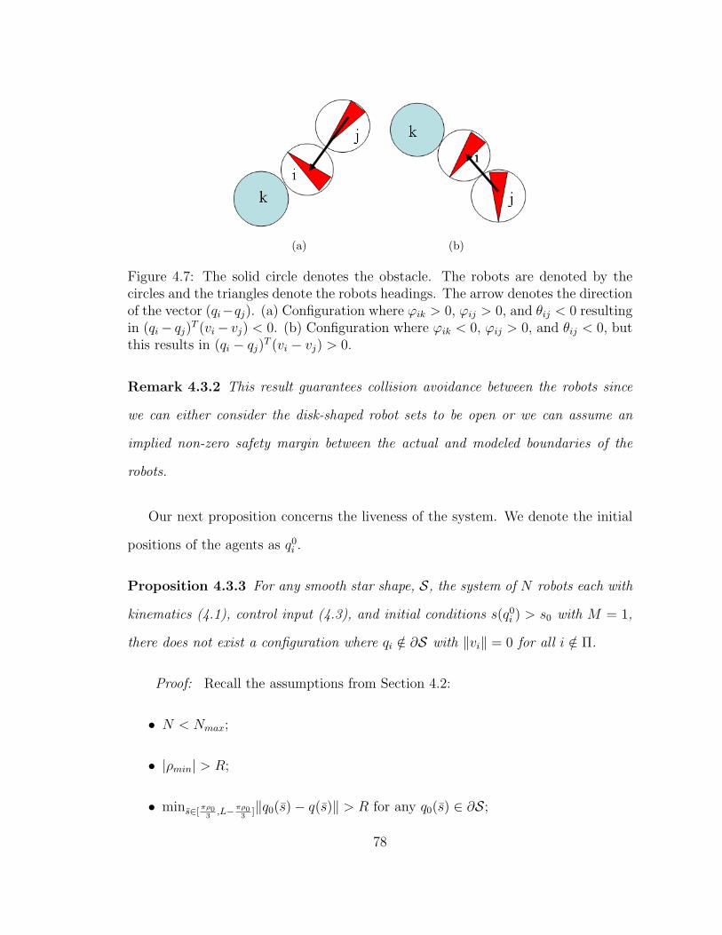
(a) (b)

Figure 4.7: The solid circle denotes the obstacle. The robots are denoted by thecircles and the triangles denote the robots headings. The arrow denotes the directionof the vector (qi−qj). (a) Configuration where ϕik > 0, ϕij > 0, and θij < 0 resultingin (qi− qj)T (vi− vj) < 0. (b) Configuration where ϕik < 0, ϕij > 0, and θij < 0, butthis results in (qi − qj)T (vi − vj) > 0.

Remark 4.3.2 This result guarantees collision avoidance between the robots since

we can either consider the disk-shaped robot sets to be open or we can assume an

implied non-zero safety margin between the actual and modeled boundaries of the

robots.

Our next proposition concerns the liveness of the system. We denote the initial

positions of the agents as q0i .

Proposition 4.3.3 For any smooth star shape, S, the system of N robots each with

kinematics (4.1), control input (4.3), and initial conditions s(q0i ) > s0 with M = 1,

there does not exist a configuration where qi /∈ ∂S with ‖vi‖ = 0 for all i /∈ Π.

Proof: Recall the assumptions from Section 4.2:

• N < Nmax;

• |ρmin| > R;

• mins∈[πρ03,L−πρ0

3]‖q0(s)− q(s)‖ > R for any q0(s) ∈ ∂S;

78

• for any i ∈ Π, d(qi, ∂S) > (R + r);

• for any i ∈ Π, d(qi, ∂W) > 3r; and

• min d(∂S, ∂W) > 2Nr.

Assume there exist is a set of agents k, . . . , l such that ‖vi‖ = 0 for all i ∈ k, . . . , l.

Let qmin = arg mini ϕ(qi). If ϕ(qmin) 6= 0, then there must exist a j ∈ Γmin and

j ∈ k, . . . , l such that ϕj < ϕi. Since ϕi is the minimum in the set k, . . . , l, this

means qmin was stopped because ϕj > ϕi, however this would violate the conditions

|ρmin| > R and mins∈[πρ03,L−πρ0

3]‖q0(s) − q(s)‖ > R. Similarly, in the tangential

direction, let qmax = arg maxi θi. Since qmax has the maximum θ in the set k, . . . , l,

qmax was stopped because there exists a j ∈ Γmax such that θj < θmax. However,

this would violate the condition N < Nmax. If qmin ∈ Π, for the set of agents to be

immobilized, this would require either d(qmin, ∂S) <= (R + r), d(qmin, ∂W) <= 3r,

min d(∂S, ∂W) < 2Nr, which violates our assumptions. Thus, there always exists

at least one agent whose velocity is non–zero.

Our next proposition concerns the convergence of the system to the desired

boundary.

Proposition 4.3.4 For any smooth star shape, S, the system of N robots each with

kinematics (4.1), control input (4.3), and initial conditions s(q0i ) > s0 for all i with

no obstacles, the system converges asymptotically to ∂S.

Proof: To show that the system converges asymptotically to ∂S, we first

consider the stability of the proposed controller. Consider the following positive

semi-definite function:

V (q) =∑i

ϕ(qi). (4.9)

79

Since D is compact, then by continuity of V , the level sets of ϕ are compact subsets

of W . Then the time derivative of V is given by

V =∑i

∇ϕ(qi)T qi

=∑i

∇iϕ(qi)T (−∇iϕif(Ni)− (∇i × ψ)g(Ti))

By construction, ∇ϕ is orthogonal to ∇×ψ, therefore the above equation simplifies

to

V =∑i

−‖∇iϕi‖2fi(Ni). (4.10)

Since f(·) ∈ [0, 1], V ≤ 0. Thus, the system N agents with kinematics (4.1) and

feedback control (4.8) is stable and approaches the largest invariant set inside ΩI =

q ∈ Q|V (q) = 0.

By Proposition 4.3.3, the closed loop system does not admit stationary points,

i.e. points where q = 0 as long as s(qi) > s0 for all i = 1, . . . , N . Since there can be

no stationary points, we conclude that V = 0 in (4.10) if and only if ∇iϕi = 0 for

all i. For a star shape, with ϕ given by (4.2), ∇ϕ = 0 if and only if q ∈ ∂S ∈ W .

Thus, the system of N robots converges asymptotically to ∂S.

The above proposition can be extended to include the obstacle avoidance case,

i.e. the controller given by (4.8) if we assume |Π| = M = 1.

Proposition 4.3.5 For any smooth star shape, S, the system of N robots each with

kinematics (4.1), control input (4.8), M = 1, and initial conditions s(q0i ) > s0 for

all i, the system converges asymptotically to ∂S.

Proof: We begin by first showing stability. Consider the function given by

80

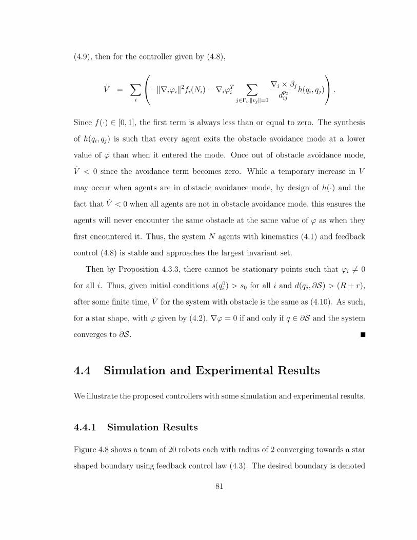
(4.9), then for the controller given by (4.8),

V =∑i

−‖∇iϕi‖2fi(Ni)−∇iϕTi

∑j∈Γi,‖vj‖=0

∇i × βjdp2ij

h(qi, qj)

.

Since f(·) ∈ [0, 1], the first term is always less than or equal to zero. The synthesis

of h(qi, qj) is such that every agent exits the obstacle avoidance mode at a lower

value of ϕ than when it entered the mode. Once out of obstacle avoidance mode,

V < 0 since the avoidance term becomes zero. While a temporary increase in V

may occur when agents are in obstacle avoidance mode, by design of h(·) and the

fact that V < 0 when all agents are not in obstacle avoidance mode, this ensures the

agents will never encounter the same obstacle at the same value of ϕ as when they

first encountered it. Thus, the system N agents with kinematics (4.1) and feedback

control (4.8) is stable and approaches the largest invariant set.

Then by Proposition 4.3.3, there cannot be stationary points such that ϕi 6= 0

for all i. Thus, given initial conditions s(q0i ) > s0 for all i and d(qj, ∂S) > (R + r),

after some finite time, V for the system with obstacle is the same as (4.10). As such,

for a star shape, with ϕ given by (4.2), ∇ϕ = 0 if and only if q ∈ ∂S and the system

converges to ∂S.

4.4 Simulation and Experimental Results

We illustrate the proposed controllers with some simulation and experimental results.

4.4.1 Simulation Results

Figure 4.8 shows a team of 20 robots each with radius of 2 converging towards a star

shaped boundary using feedback control law (4.3). The desired boundary is denoted

81

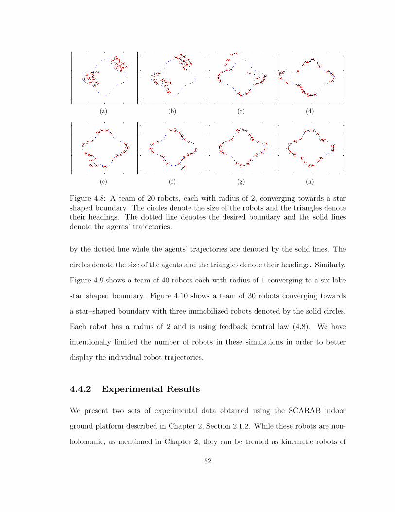
(a) (b) (c) (d)

(e) (f) (g) (h)

Figure 4.8: A team of 20 robots, each with radius of 2, converging towards a starshaped boundary. The circles denote the size of the robots and the triangles denotetheir headings. The dotted line denotes the desired boundary and the solid linesdenote the agents’ trajectories.

by the dotted line while the agents’ trajectories are denoted by the solid lines. The

circles denote the size of the agents and the triangles denote their headings. Similarly,

Figure 4.9 shows a team of 40 robots each with radius of 1 converging to a six lobe

star–shaped boundary. Figure 4.10 shows a team of 30 robots converging towards

a star–shaped boundary with three immobilized robots denoted by the solid circles.

Each robot has a radius of 2 and is using feedback control law (4.8). We have

intentionally limited the number of robots in these simulations in order to better

display the individual robot trajectories.

4.4.2 Experimental Results

We present two sets of experimental data obtained using the SCARAB indoor

ground platform described in Chapter 2, Section 2.1.2. While these robots are non-

holonomic, as mentioned in Chapter 2, they can be treated as kinematic robots of

82

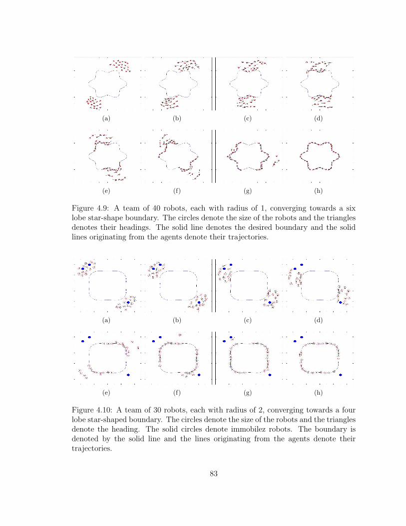
(a) (b) (c) (d)

(e) (f) (g) (h)

Figure 4.9: A team of 40 robots, each with radius of 1, converging towards a sixlobe star-shape boundary. The circles denote the size of the robots and the trianglesdenotes their headings. The solid line denotes the desired boundary and the solidlines originating from the agents denote their trajectories.

(a) (b) (c) (d)

(e) (f) (g) (h)

Figure 4.10: A team of 30 robots, each with radius of 2, converging towards a fourlobe star-shaped boundary. The circles denote the size of the robots and the trianglesdenote the heading. The solid circles denote immobilez robots. The boundary isdenoted by the solid line and the lines originating from the agents denote theirtrajectories.

83

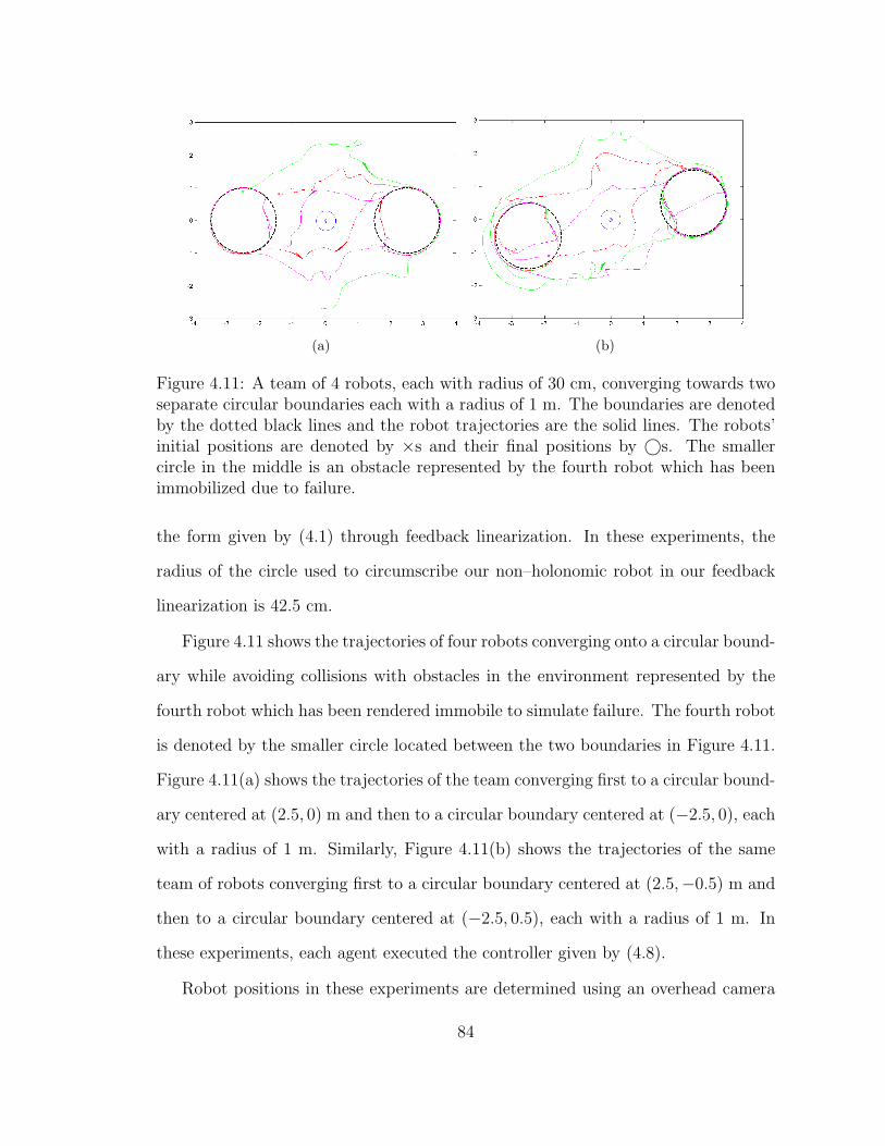
(a) (b)

Figure 4.11: A team of 4 robots, each with radius of 30 cm, converging towards twoseparate circular boundaries each with a radius of 1 m. The boundaries are denotedby the dotted black lines and the robot trajectories are the solid lines. The robots’initial positions are denoted by ×s and their final positions by ©s. The smallercircle in the middle is an obstacle represented by the fourth robot which has beenimmobilized due to failure.

the form given by (4.1) through feedback linearization. In these experiments, the

radius of the circle used to circumscribe our non–holonomic robot in our feedback

linearization is 42.5 cm.

Figure 4.11 shows the trajectories of four robots converging onto a circular bound-

ary while avoiding collisions with obstacles in the environment represented by the

fourth robot which has been rendered immobile to simulate failure. The fourth robot

is denoted by the smaller circle located between the two boundaries in Figure 4.11.

Figure 4.11(a) shows the trajectories of the team converging first to a circular bound-

ary centered at (2.5, 0) m and then to a circular boundary centered at (−2.5, 0), each

with a radius of 1 m. Similarly, Figure 4.11(b) shows the trajectories of the same

team of robots converging first to a circular boundary centered at (2.5,−0.5) m and

then to a circular boundary centered at (−2.5, 0.5), each with a radius of 1 m. In

these experiments, each agent executed the controller given by (4.8).

Robot positions in these experiments are determined using an overhead camera

84

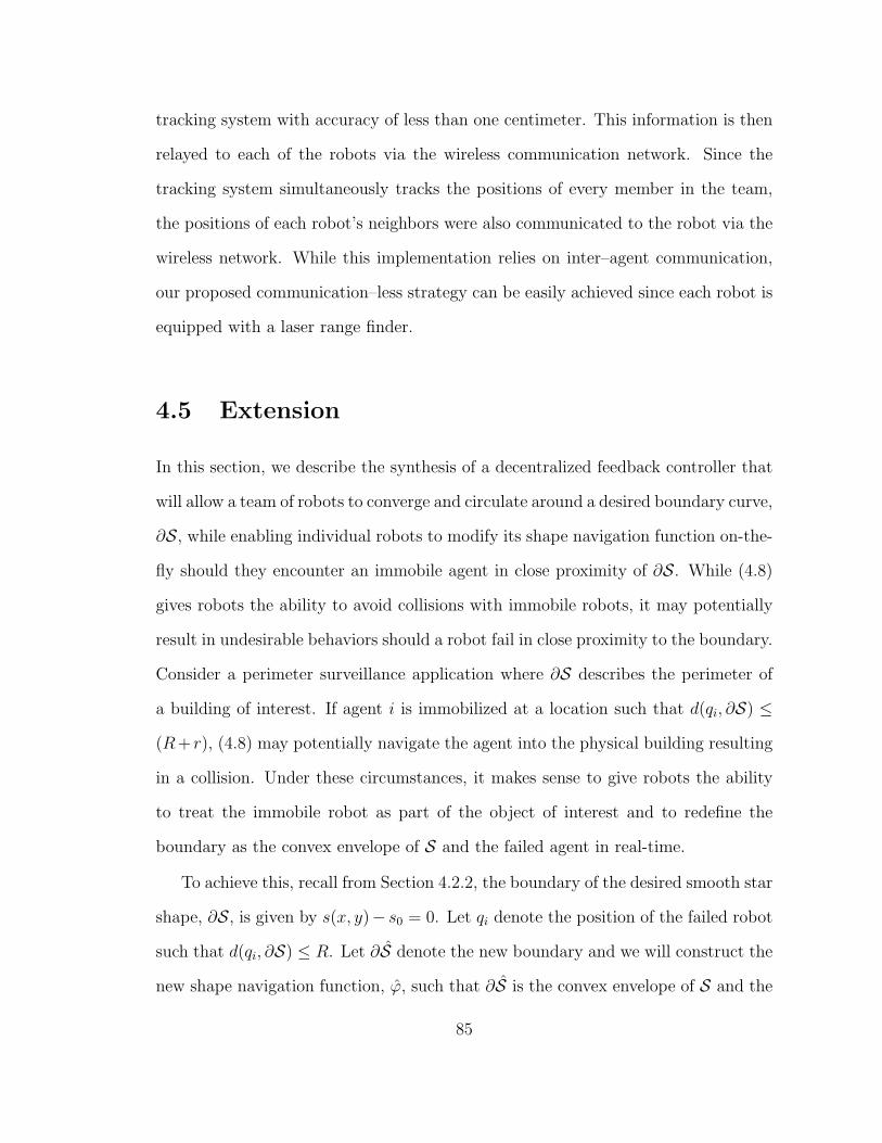
tracking system with accuracy of less than one centimeter. This information is then

relayed to each of the robots via the wireless communication network. Since the

tracking system simultaneously tracks the positions of every member in the team,

the positions of each robot’s neighbors were also communicated to the robot via the

wireless network. While this implementation relies on inter–agent communication,

our proposed communication–less strategy can be easily achieved since each robot is

equipped with a laser range finder.

4.5 Extension

In this section, we describe the synthesis of a decentralized feedback controller that

will allow a team of robots to converge and circulate around a desired boundary curve,

∂S, while enabling individual robots to modify its shape navigation function on-the-

fly should they encounter an immobile agent in close proximity of ∂S. While (4.8)

gives robots the ability to avoid collisions with immobile robots, it may potentially

result in undesirable behaviors should a robot fail in close proximity to the boundary.

Consider a perimeter surveillance application where ∂S describes the perimeter of

a building of interest. If agent i is immobilized at a location such that d(qi, ∂S) ≤

(R+ r), (4.8) may potentially navigate the agent into the physical building resulting

in a collision. Under these circumstances, it makes sense to give robots the ability

to treat the immobile robot as part of the object of interest and to redefine the

boundary as the convex envelope of S and the failed agent in real-time.

To achieve this, recall from Section 4.2.2, the boundary of the desired smooth star

shape, ∂S, is given by s(x, y)− s0 = 0. Let qi denote the position of the failed robot

such that d(qi, ∂S) ≤ R. Let ∂S denote the new boundary and we will construct the

new shape navigation function, ϕ, such that ∂S is the convex envelope of S and the

85

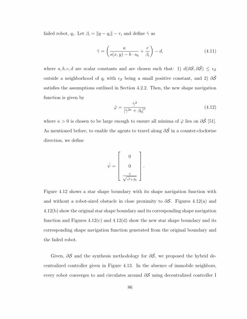
failed robot, qi. Let βi = ‖q − qi‖ − ri and define γ as

γ =

(a

s(x, y)− b · s0

+c

βi

)− d, (4.11)

where a, b, c, d are scalar constants and are chosen such that: 1) d(∂S, ∂S) ≤ εS

outside a neighborhood of qi with εS being a small positive constant, and 2) ∂S

satisfies the assumptions outlined in Section 4.2.2. Then, the new shape navigation

function is given by

ϕ =γ2

[γ2κ + β0]κ(4.12)

where κ > 0 is chosen to be large enough to ensure all minima of ϕ lies on ∂S [51].

As mentioned before, to enable the agents to travel along ∂S in a counter-clockwise

direction, we define

ψ =

0

0

γ√γ2+β0

.

Figure 4.12 shows a star shape boundary with its shape navigation function with

and without a robot-sized obstacle in close proximity to ∂S. Figures 4.12(a) and

4.12(b) show the original star shape boundary and its corresponding shape navigation

function and Figures 4.12(c) and 4.12(d) show the new star shape boundary and its

corresponding shape navigation function generated from the original boundary and

the failed robot.

Given, ∂S and the synthesis methodology for ∂S, we proposed the hybrid de-

centralized controller given in Figure 4.13. In the absence of immobile neighbors,

every robot converges to and circulates around ∂S using decentralized controller I

86

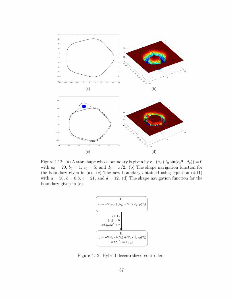
(a) (b)

(c) (d)

Figure 4.12: (a) A star shape whose boundary is given by r−(a0+b0 sin(c0θ+d0)) = 0with a0 = 20, b0 = 1, c0 = 5, and d0 = π/2. (b) The shape navigation function forthe boundary given in (a). (c) The new boundary obtained using equation (4.11)with a = 50, b = 0.8, c = 21, and d = 12. (d) The shape navigation function for theboundary given in (c).

Figure 4.13: Hybrid decentralized controller.

87

in Figure 4.13, i.e. control input (4.3). Each robot then updates its control input to

controller II in Figure 4.13 based on the first time it detects the immobile neighbor.

Once a failed robot is detected in close proximity of ∂S, the new shape navigation

function, ϕ, is activated and the old shape navigation function, ϕ, discarded. We

note this controller only switches once and the switch occurs the first time the failed

robot is detected. Lastly, to ensure avoidance of failed robots away from the desired

boundary, the third term in equation (4.8) can be included.

The stability and convergence results in Section 4.3 can be extended for the

control input described in Figure 4.13. Since the particular controller switches from

one shape navigation function to another and the switch only occurs once, the time

derivative for the positive semi–definite function V given by (4.9) is simply given by

(4.10), where ϕ denotes the appropriate shape function. Furthermore, in the event

more and more robots fail in close proximity to the boundary, ∂S can be updated

incrementally.

4.5.1 Simulations

We illustrate this controller in this simulation with 13 robots converging to the

same star–shaped boundary as the one shown in Figure 4.10. As the team begins to

approach the boundary, one robot is immobilized in close proximity to the boundary.

In this figure the broken robot is denoted by the solid circle.

4.6 Conclusions and Future Work

In this chapter, we have presented an efficient decentralized approach for a team

of robots to converge and track the boundary of a desired two-dimensional shape

while avoiding collisions. The algorithm can be used to deploy multiple robots to do

88

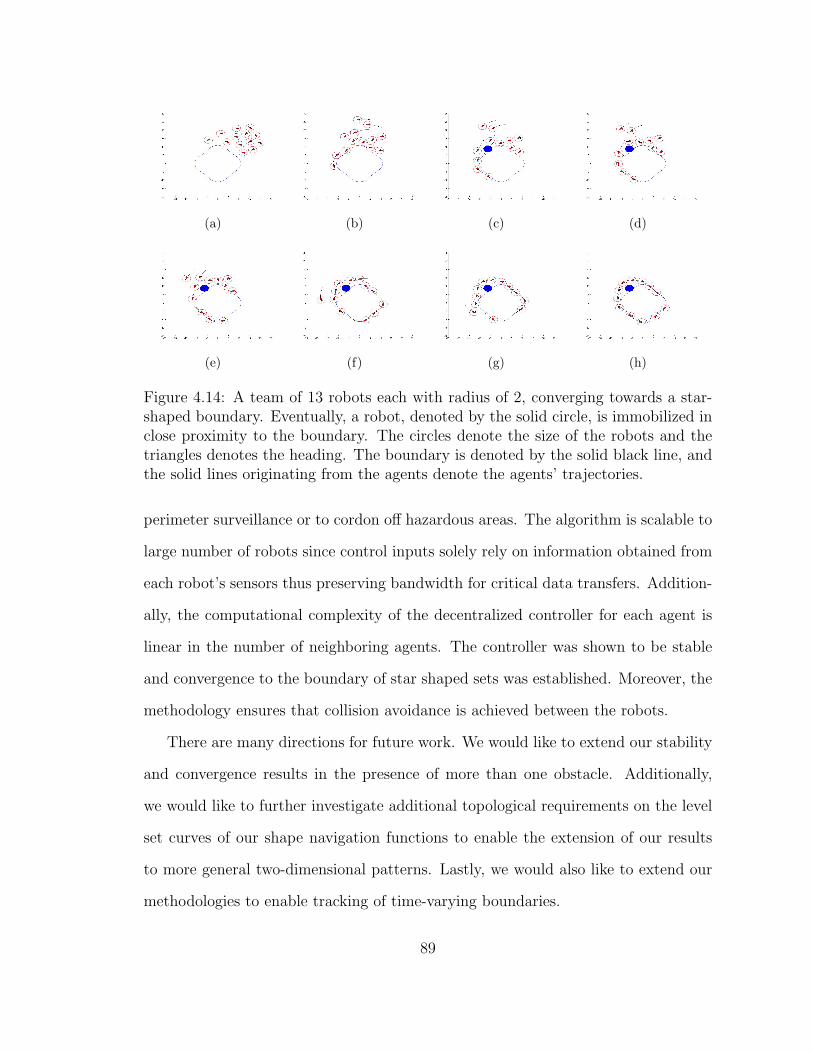
(a) (b) (c) (d)

(e) (f) (g) (h)

Figure 4.14: A team of 13 robots each with radius of 2, converging towards a star-shaped boundary. Eventually, a robot, denoted by the solid circle, is immobilized inclose proximity to the boundary. The circles denote the size of the robots and thetriangles denotes the heading. The boundary is denoted by the solid black line, andthe solid lines originating from the agents denote the agents’ trajectories.

perimeter surveillance or to cordon off hazardous areas. The algorithm is scalable to

large number of robots since control inputs solely rely on information obtained from

each robot’s sensors thus preserving bandwidth for critical data transfers. Addition-

ally, the computational complexity of the decentralized controller for each agent is

linear in the number of neighboring agents. The controller was shown to be stable

and convergence to the boundary of star shaped sets was established. Moreover, the

methodology ensures that collision avoidance is achieved between the robots.

There are many directions for future work. We would like to extend our stability

and convergence results in the presence of more than one obstacle. Additionally,

we would like to further investigate additional topological requirements on the level

set curves of our shape navigation functions to enable the extension of our results

to more general two-dimensional patterns. Lastly, we would also like to extend our

methodologies to enable tracking of time-varying boundaries.

89

Chapter 5

Decentralized Controllers for

Shape Generation with Robotic

Swarms

Similar to the previous chapter, this chapter considers motion control strategies for

robotic swarms in applications such as surveillance monitoring of specified areas, sur-

rounding large objects for capture or for manipulation, and cordoning off hazardous

regions after chemical spills or biological terrorist attacks. The work presented here

is an initial attempt to extend the results presented in the previous chapter to second

order systems.

This chapter builds on the results of Chaimowicz et al. [17] and Hsieh et al. [40]

and considers not only the pattern generation problem, but the pattern generation

problem with inter–agent constraints. This work is similar in spirit to the works by

Belta, Chaimowicz, and Michael [10, 16, 57], where we address the synthesis of de-

centralized controllers that guarantees the convergence of the team to the boundary

of some desired shape as well as the stability of the resulting formation, all the while

90

maintaining inter-agent constraints through local interactions.

We formulate the problem in Section 5.1 and present our methodology in 5.2.

The stability and convergence properties of the controller are discussed in Section

5.3 with simulation results presented in Section 5.4. This chapter concludes with

Section 5.5.

5.1 Problem Formulation

Assume a swarm of N planar fully actuated robots each with the following dynamics,

qi = vi (5.1a)

vi = ui (5.1b)

where qi = (xi, yi)T , vi, and ui respectively denote the ith agent’s position, velocity,

and control input. Thus, the robot state is a 4 × 1 state vector xi =[qTi v

Ti

]T. We

define the configuration space as Q ⊂ R2N , and the configuration of the swarm of

robots as given by q =[qT1 . . . q

TN

]T ∈ Q. Similarly, the state space vector is given

by x =[xT1 . . .x

TN

]T ∈ X ⊂ R4N . In general, we consider all systems of N agents

whose individual dynamics can be transformed into (5.1) via some diffeomorphic

state transformation.

Our goal is to design control inputs that will drive the group of N robots to

the boundary (curve) of a desired smooth, compact set, i.e. shape, while main-

taining inter-robot constraints. This is relevant for applications such as perimeter

surveillance or surrounding an object for capture and/or transportation. Thus, the

controller synthesis problem for pattern generation is to find a controller that can

drive the team to the desired boundary while:

91

[P1] avoiding collisions with other agents, and/or

[P2] maintaining specified proximity constraints with other agents, such as for com-

munication maintenance.

We outline our methodology in the following section.

5.2 Methodology

5.2.1 Assumptions and Definitions

For a given desired shape, S, whose boundary is denoted by ∂S, assume ∂S is a two

dimensional planar curve in an obstacle–free workspace that can be described by an

implicit function, s(x, y) = 0. In general, we will assume that the boundary curves

of interest are regular closed, simple, smooth planar curves enclosing star shaped

sets. The regular and simple assumptions are necessary to ensure that the closed

curves do not self intersect [29].

In situations where it is important that the team maintains a connected com-

munication network or specific team members remain within a prescribed range of

one another to enable grasping of objects for transportation/manipulation, we will

further require the team to maintain a desired interconnection topology. We use a

proximity graph, G = (V , E), to model the inter-robot constraints, where V and E

denote the set of vertices and edges of G. Each robot is then represented by a vertex

in V and proximity relations between pairs of robots are represented by the edges in

E . As such, for any two robots represented by a, b ∈ V , we say a and b are adjacent or

neighbors, denoted by a ∼ b, if a is in the neighborhood of b and b is in the neighbor-

hood of a, and as such the edge (a, b) ∈ E . In our analysis, robot i’s neighborhood

is defined as the ball given by Bi = q| ‖qi − q‖ ≤ d, where d > 0 denotes the

92

interaction range. For the constraints under consideration, we choose d = δ for col-

lision avoidance and d = ∆ for proximity maintenance such that δ < ∆. In practice,

whether for collision avoidance or proximity maintenance, this prescribed range can

be determined based on the communication and/or sensing hardware, performance

requirements within a given environment, and/or experimental results. Thus, for

any proximity graph G, the the N ×N adjacency matrix is defined as:

Aij =

1 if j ∈ Γi

0 otherwise.

Given a set of inter-agent constraints, we encode the information in a desired

proximity graph, Gd, such that every inter-agent constraint is represented by an edge.

Thus, the graph Gd represents the desired interconnection topology and we denote its

associated adjacency matrix as Ad. We will assume that the desired proximity graph

is always a subgraph of the initial proximity graph to ensure the team initializes in

a feasible configuration.

Lastly, since our goal is to synthesize decentralized controllers that will allow a

team of robots to converge to the boundary while satisfying inter-agent constraints,

we note that given d > 0, the length of ∂S naturally imposes an upper bound on

the number of robots, denoted by e.g. Nmax > 0, that can fit on the boundary.

Similarly, the length of the boundary will naturally impose a lower bound, Nmin, on

the number of robots that can effectively cover the desired boundary given a fixed

sensing range.1

1Given an interaction range or a fixed sensing radius d > 0, Nmin and Nmax can be determinedpurely geometrically. To accomplish this, begin by selecting an initial point on ∂S and placinga circle of radius d centered at this point. Next, select another point on ∂S by going along theboundary in a counter-clockwise direction. Select this next point such that a circle of radius dcentered at this second point is tangent to the first circle. By repeating this process, one willbe able to generate a sequence of circles centered at points on the boundary that are tangent to

93

In this work, we are primarily concerned with convergence to the desired bound-

ary and as such we will make the following additional assumptions:

1. N < Nmax;

2. |ρmin| > δ, where ρmin denotes the smallest radius of curvature of ∂S;

3. mins∈[πρ02,L−πρ0

2]‖q0(s)− q(s)‖ > δ for any q0(s) ∈ ∂S, where s ∈ [0, L] denotes

the arclength and ρ0 denotes the radius of curvature at q0.

Assumption 1 ensures all agents with finite interaction range will be able to converge

to the desired boundary while satisfying all constraints. Assumptions 2 and 3 ensure

convergence by excluding boundaries with sharp turns and star shapes with narrow

passages, e.g. hourglass shapes, that may result in robots repelling each other away

from the boundary when avoiding collisions. These are similar to those presented

in Chapter 4 and as such, we refer the reader to Chapter 4 for the more detailed

discussion on them.

5.2.2 Controller Synthesis

Shape Functions

For a desired shape, S, we define the shape function, f : R2 → R, such that f is

positive semi-definite in Q and for all (x, y) ∈ ∂S, i.e. points on the curve s(x, y) = 0,

f(x, y) = 0. In general, for any parameterization s(x, y) = 0, f = (s(x, y))2 is a

candidate shape function. For star shapes, we choose f = s2 such that

1. s(x, y) is at least twice differentiable on Q; and

one another. Since the boundary and the d are both finite, one can continue this process untilone can no longer fit a circle centered at a point on ∂S without intersecting any of the previouscircles. Thus, the number of tangent circles drawn at the end of the process gives Nmax. A similarprocedure can be used to determine Nmin.

94

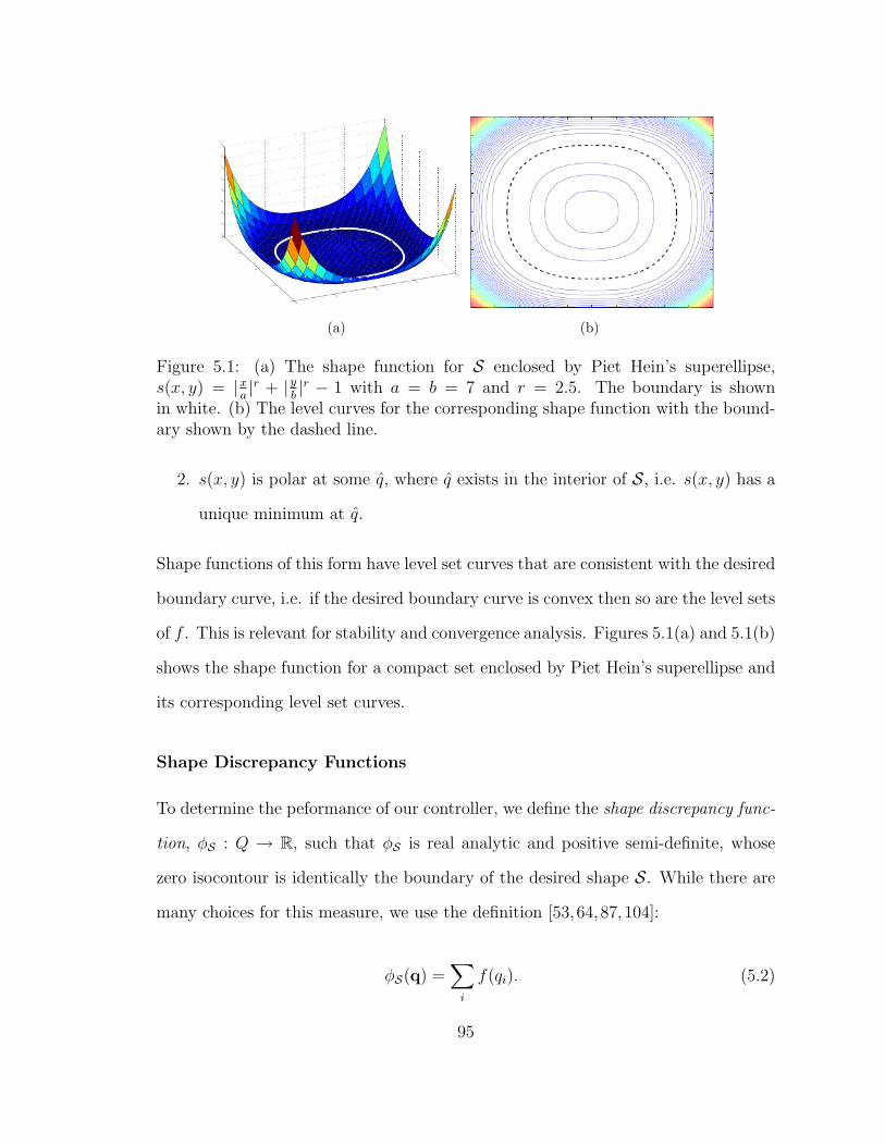
(a) (b)

Figure 5.1: (a) The shape function for S enclosed by Piet Hein’s superellipse,s(x, y) = |x

a|r + |y

b|r − 1 with a = b = 7 and r = 2.5. The boundary is shown

in white. (b) The level curves for the corresponding shape function with the bound-ary shown by the dashed line.

2. s(x, y) is polar at some q, where q exists in the interior of S, i.e. s(x, y) has a

unique minimum at q.

Shape functions of this form have level set curves that are consistent with the desired

boundary curve, i.e. if the desired boundary curve is convex then so are the level sets

of f . This is relevant for stability and convergence analysis. Figures 5.1(a) and 5.1(b)

shows the shape function for a compact set enclosed by Piet Hein’s superellipse and

its corresponding level set curves.

Shape Discrepancy Functions

To determine the peformance of our controller, we define the shape discrepancy func-

tion, φS : Q → R, such that φS is real analytic and positive semi-definite, whose

zero isocontour is identically the boundary of the desired shape S. While there are

many choices for this measure, we use the definition [53,64,87,104]:

φS(q) =∑i

f(qi). (5.2)

95

Thus, the shape discrepancy function provides a measure of how close the team is

to ∂S.

Controller

For the system of N robots with dynamics given by equation (5.1), consider the

following feedback policy for each robot

ui = −∇if(qi)− c vi −∑

j s.t. Adij=1

∇igij(‖qij‖) (5.3)

where c > 0 is a constant scalar and qij = qi − qj. The first term of (5.3) drives

the agent towards the desired curve while the second term adds damping to the

system. The function gij(‖qij‖) in the third term is an artificial potential function

whose gradient models the interactions between each robot and its neighbors in the

neighborhood given by Bi. In the remainder of the paper, we will denote gij(‖qij‖) as

simply gij. Lastly, ∇i denotes the partial derivatives with respect to the coordinates

of the ith robot.

For collision avoidance, i.e. [P1] in Section 5.1, consider the following candidate

function for gij:

gij =1

(‖qij‖)k1(5.4)

where the postive even scalar k1 is chosen such that the interaction forces are negli-

gible when ‖qij‖ > δ and repulsive when 0 < ‖qij‖ ≤ δ, thus ensuring collisions do

not occur. Similarly, when the maintenance of a specific proximity graph is required,

i.e. [P2], consider the following candidate function:

gij =1

(∆− ‖qij‖)k2(5.5)

96

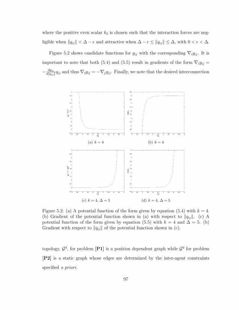
where the positive even scalar k2 is chosen such that the interaction forces are neg-

ligible when ‖qij‖ < ∆− ε and attractive when ∆− ε ≤ ‖qij‖ ≤ ∆, with 0 < ε < ∆.

Figure 5.2 shows candidate functions for gij with the corresponding ∇igij. It is

important to note that both (5.4) and (5.5) result in gradients of the form ∇igij =

− dgijd‖qij‖qij and thus ∇igij = −∇jgij. Finally, we note that the desired interconnection

(a) k = 4 (b) k = 4

(c) k = 4, ∆ = 5 (d) k = 4, ∆ = 5

Figure 5.2: (a) A potential function of the form given by equation (5.4) with k = 4.(b) Gradient of the potential function shown in (a) with respect to ‖qij‖. (c) Apotential function of the form given by equation (5.5) with k = 4 and ∆ = 5. (b)Gradient with respect to ‖qij‖ of the potential function shown in (c).

topology, Gd, for problem [P1] is a position dependent graph while Gd for problem

[P2] is a static graph whose edges are determined by the inter-agent constraints

specified a priori.

97

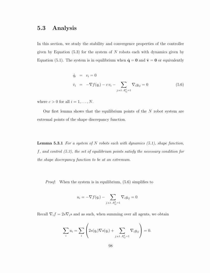
5.3 Analysis

In this section, we study the stability and convergence properties of the controller

given by Equation (5.3) for the system of N robots each with dynamics given by

Equation (5.1). The system is in equilibrium when q = 0 and v = 0 or equivalently

qi = vi = 0

vi = −∇f(qi)− c vi −∑

j s.t. Adij=1

∇igij = 0 (5.6)

where c > 0 for all i = 1, . . . , N .

Our first lemma shows that the equilibrium points of the N robot system are

extremal points of the shape discrepancy function.

Lemma 5.3.1 For a system of N robots each with dynamics (5.1), shape function,

f , and control (5.3), the set of equilibrium points satisfy the necessary condition for

the shape discrepancy function to be at an extremum.

Proof: When the system is in equilibrium, (5.6) simplifies to

ui = −∇f(qi)−∑

j s.t. Adij=1

∇igij = 0

Recall ∇if = 2s∇is and as such, when summing over all agents, we obtain

∑i

ui =∑i

2s(qi)∇s(qi) +∑

j s.t. Adij=1

∇igij

= 0.

98

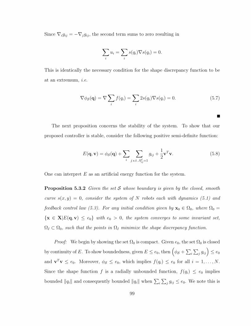
Since ∇igij = −∇jgij, the second term sums to zero resulting in

∑i

ui =∑i

s(qi)∇s(qi) = 0.

This is identically the necessary condition for the shape discrepancy function to be

at an extremum, i.e.

∇φS(q) = ∇∑i

f(qi) =∑i

2s(qi)∇s(qi) = 0. (5.7)

The next proposition concerns the stability of the system. To show that our

proposed controller is stable, consider the following positive semi-definite function:

E(q,v) = φS(q) +∑i

∑j s.t. Adij=1

gij +1

2vTv. (5.8)

One can interpret E as an artificial energy function for the system.

Proposition 5.3.2 Given the set S whose boundary is given by the closed, smooth

curve s(x, y) = 0, consider the system of N robots each with dynamics (5.1) and

feedback control law (5.3). For any initial condition given by x0 ∈ Ω0, where Ω0 =

x ∈ X|E(q,v) ≤ e0 with e0 > 0, the system converges to some invariant set,

ΩI ⊂ Ω0, such that the points in ΩI minimize the shape discrepancy function.

Proof: We begin by showing the set Ω0 is compact. Given e0, the set Ω0 is closed

by continuity of E. To show boundedness, given E ≤ e0, then(φS +

∑i

∑j gij

)≤ e0

and vTv ≤ e0. Moreover, φS ≤ e0, which implies f(qi) ≤ e0 for all i = 1, . . . , N .

Since the shape function f is a radially unbounded function, f(qi) ≤ e0 implies

bounded ‖qi‖ and consequently bounded ‖qi‖ when∑

i

∑j gij ≤ e0. We note this is

99

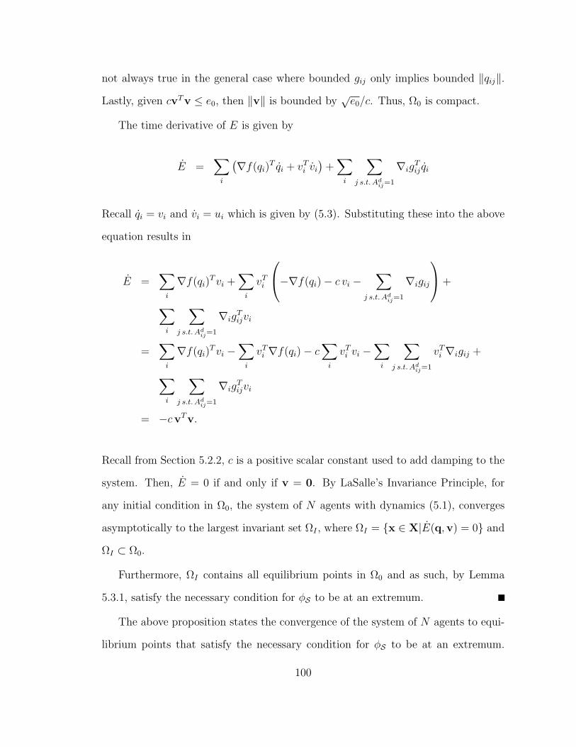
not always true in the general case where bounded gij only implies bounded ‖qij‖.

Lastly, given cvTv ≤ e0, then ‖v‖ is bounded by√e0/c. Thus, Ω0 is compact.

The time derivative of E is given by

E =∑i

(∇f(qi)

T qi + vTi vi)

+∑i

∑j s.t. Adij=1

∇igTij qi

Recall qi = vi and vi = ui which is given by (5.3). Substituting these into the above

equation results in

E =∑i

∇f(qi)Tvi +

∑i

vTi

−∇f(qi)− c vi −∑

j s.t. Adij=1

∇igij

+

∑i

∑j s.t. Adij=1

∇igTijvi

=∑i

∇f(qi)Tvi −

∑i

vTi ∇f(qi)− c∑i

vTi vi −∑i

∑j s.t. Adij=1

vTi ∇igij +

∑i

∑j s.t. Adij=1

∇igTijvi

= −cvTv.

Recall from Section 5.2.2, c is a positive scalar constant used to add damping to the

system. Then, E = 0 if and only if v = 0. By LaSalle’s Invariance Principle, for

any initial condition in Ω0, the system of N agents with dynamics (5.1), converges

asymptotically to the largest invariant set ΩI , where ΩI = x ∈ X|E(q,v) = 0 and

ΩI ⊂ Ω0.

Furthermore, ΩI contains all equilibrium points in Ω0 and as such, by Lemma

5.3.1, satisfy the necessary condition for φS to be at an extremum.

The above proposition states the convergence of the system of N agents to equi-

librium points that satisfy the necessary condition for φS to be at an extremum.

100

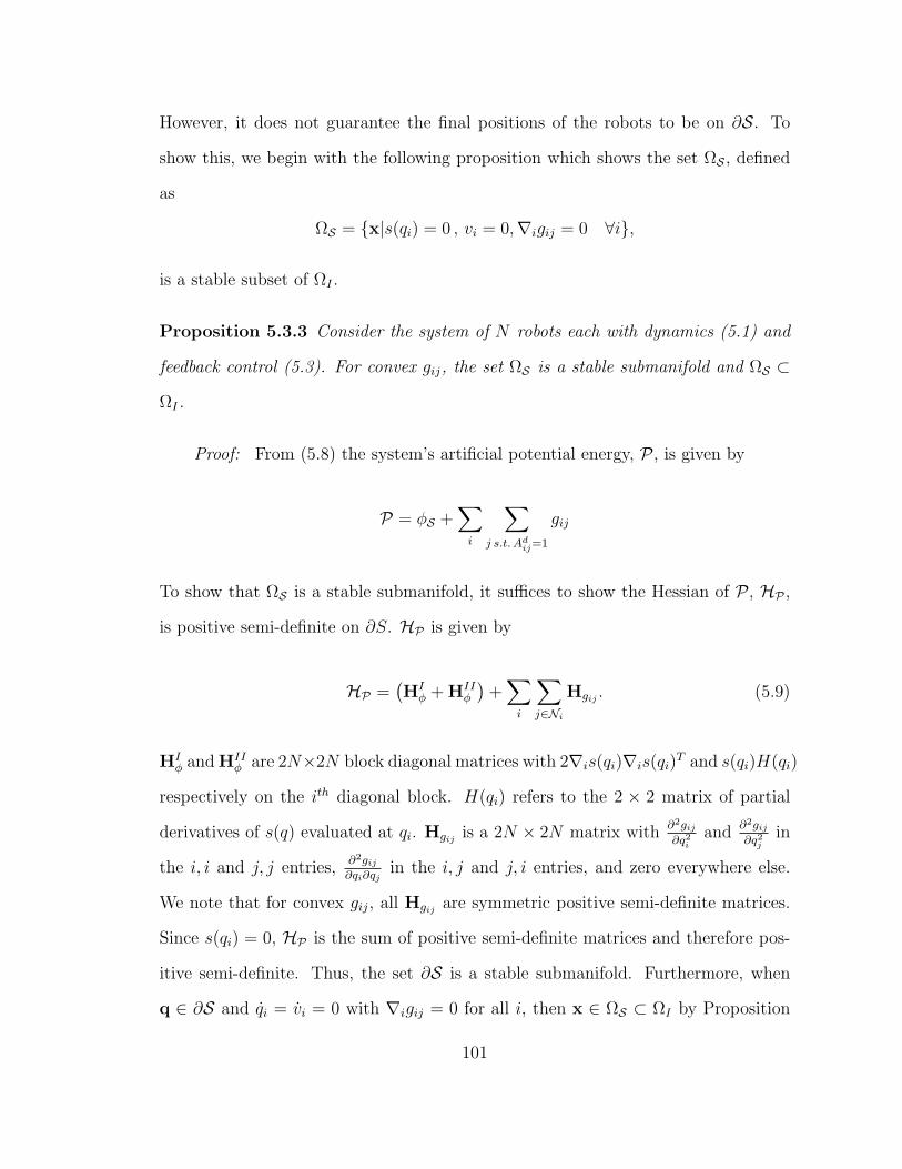
However, it does not guarantee the final positions of the robots to be on ∂S. To

show this, we begin with the following proposition which shows the set ΩS , defined

as

ΩS = x|s(qi) = 0 , vi = 0,∇igij = 0 ∀i,

is a stable subset of ΩI .

Proposition 5.3.3 Consider the system of N robots each with dynamics (5.1) and

feedback control (5.3). For convex gij, the set ΩS is a stable submanifold and ΩS ⊂

ΩI .

Proof: From (5.8) the system’s artificial potential energy, P , is given by

P = φS +∑i

∑j s.t. Adij=1

gij

To show that ΩS is a stable submanifold, it suffices to show the Hessian of P , HP ,

is positive semi-definite on ∂S. HP is given by

HP =(HIφ + HII

φ

)+∑i

∑j∈Ni

Hgij . (5.9)

HIφ and HII

φ are 2N×2N block diagonal matrices with 2∇is(qi)∇is(qi)T and s(qi)H(qi)

respectively on the ith diagonal block. H(qi) refers to the 2 × 2 matrix of partial

derivatives of s(q) evaluated at qi. Hgij is a 2N × 2N matrix with∂2gij∂q2i

and∂2gij∂q2j

in

the i, i and j, j entries,∂2gij∂qi∂qj

in the i, j and j, i entries, and zero everywhere else.

We note that for convex gij, all Hgij are symmetric positive semi-definite matrices.

Since s(qi) = 0, HP is the sum of positive semi-definite matrices and therefore pos-

itive semi-definite. Thus, the set ∂S is a stable submanifold. Furthermore, when

q ∈ ∂S and qi = vi = 0 with ∇igij = 0 for all i, then x ∈ ΩS ⊂ ΩI by Proposition

101

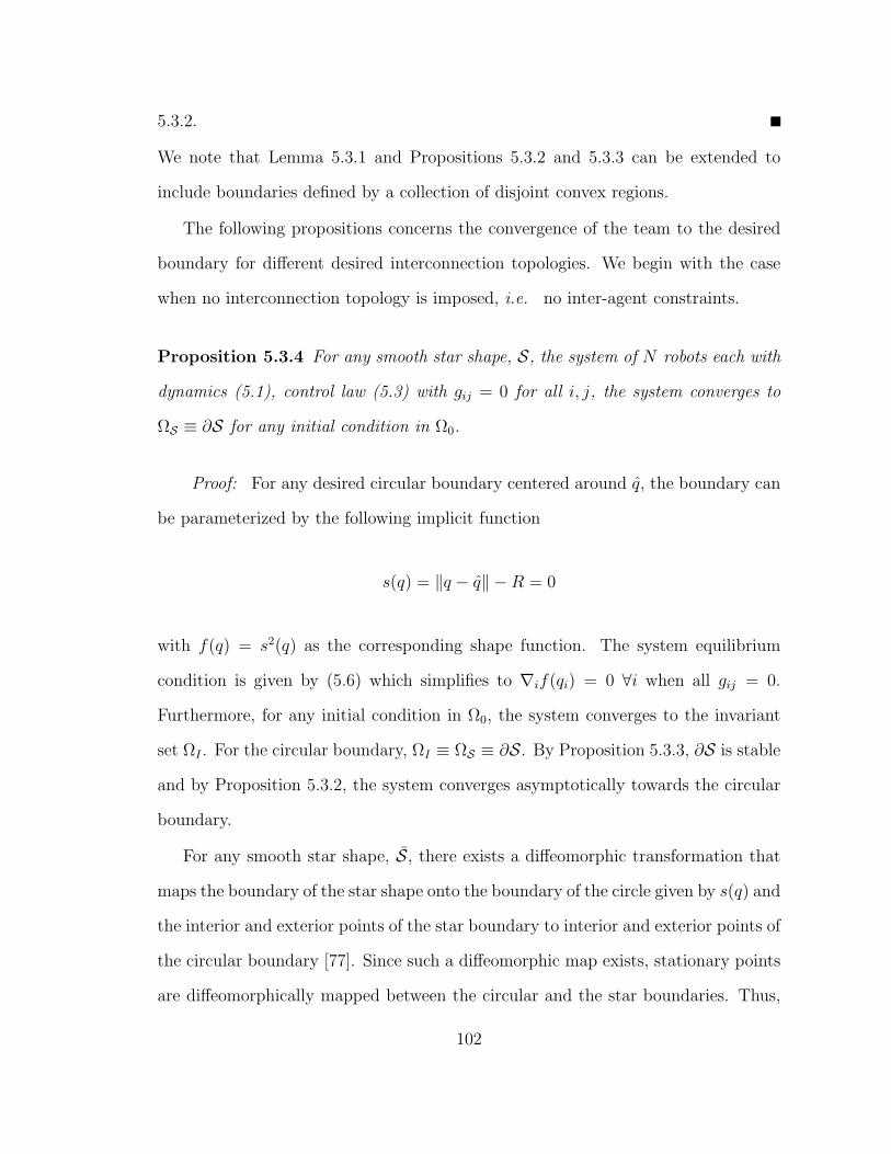
5.3.2.

We note that Lemma 5.3.1 and Propositions 5.3.2 and 5.3.3 can be extended to

include boundaries defined by a collection of disjoint convex regions.

The following propositions concerns the convergence of the team to the desired

boundary for different desired interconnection topologies. We begin with the case

when no interconnection topology is imposed, i.e. no inter-agent constraints.

Proposition 5.3.4 For any smooth star shape, S, the system of N robots each with

dynamics (5.1), control law (5.3) with gij = 0 for all i, j, the system converges to

ΩS ≡ ∂S for any initial condition in Ω0.

Proof: For any desired circular boundary centered around q, the boundary can

be parameterized by the following implicit function

s(q) = ‖q − q‖ −R = 0

with f(q) = s2(q) as the corresponding shape function. The system equilibrium

condition is given by (5.6) which simplifies to ∇if(qi) = 0 ∀i when all gij = 0.

Furthermore, for any initial condition in Ω0, the system converges to the invariant

set ΩI . For the circular boundary, ΩI ≡ ΩS ≡ ∂S. By Proposition 5.3.3, ∂S is stable

and by Proposition 5.3.2, the system converges asymptotically towards the circular

boundary.

For any smooth star shape, S, there exists a diffeomorphic transformation that

maps the boundary of the star shape onto the boundary of the circle given by s(q) and

the interior and exterior points of the star boundary to interior and exterior points of

the circular boundary [77]. Since such a diffeomorphic map exists, stationary points

are diffeomorphically mapped between the circular and the star boundaries. Thus,

102

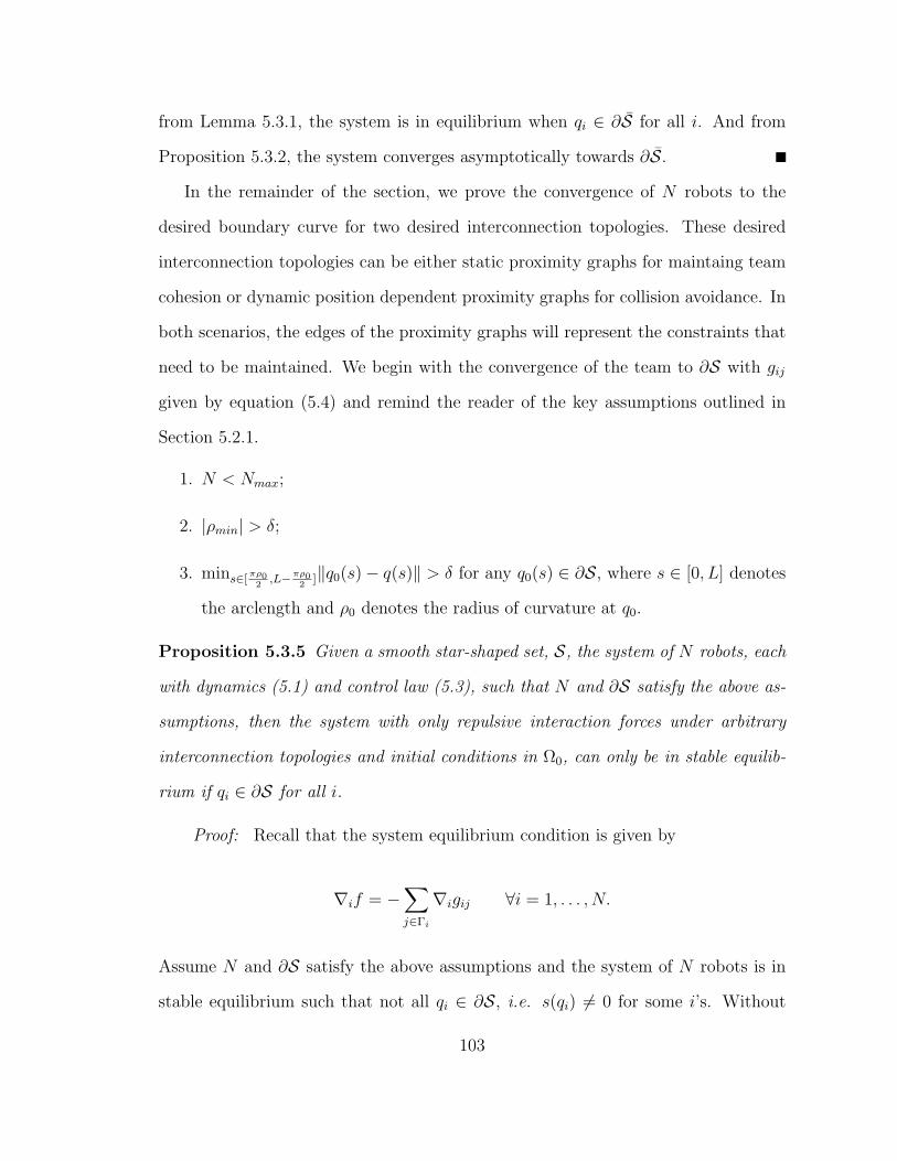
from Lemma 5.3.1, the system is in equilibrium when qi ∈ ∂S for all i. And from

Proposition 5.3.2, the system converges asymptotically towards ∂S.

In the remainder of the section, we prove the convergence of N robots to the

desired boundary curve for two desired interconnection topologies. These desired

interconnection topologies can be either static proximity graphs for maintaing team

cohesion or dynamic position dependent proximity graphs for collision avoidance. In

both scenarios, the edges of the proximity graphs will represent the constraints that

need to be maintained. We begin with the convergence of the team to ∂S with gij

given by equation (5.4) and remind the reader of the key assumptions outlined in

Section 5.2.1.

1. N < Nmax;

2. |ρmin| > δ;

3. mins∈[πρ02,L−πρ0

2]‖q0(s)− q(s)‖ > δ for any q0(s) ∈ ∂S, where s ∈ [0, L] denotes

the arclength and ρ0 denotes the radius of curvature at q0.

Proposition 5.3.5 Given a smooth star-shaped set, S, the system of N robots, each

with dynamics (5.1) and control law (5.3), such that N and ∂S satisfy the above as-

sumptions, then the system with only repulsive interaction forces under arbitrary

interconnection topologies and initial conditions in Ω0, can only be in stable equilib-

rium if qi ∈ ∂S for all i.

Proof: Recall that the system equilibrium condition is given by

∇if = −∑j∈Γi

∇igij ∀i = 1, . . . , N.

Assume N and ∂S satisfy the above assumptions and the system of N robots is in

stable equilibrium such that not all qi ∈ ∂S, i.e. s(qi) 6= 0 for some i’s. Without

103

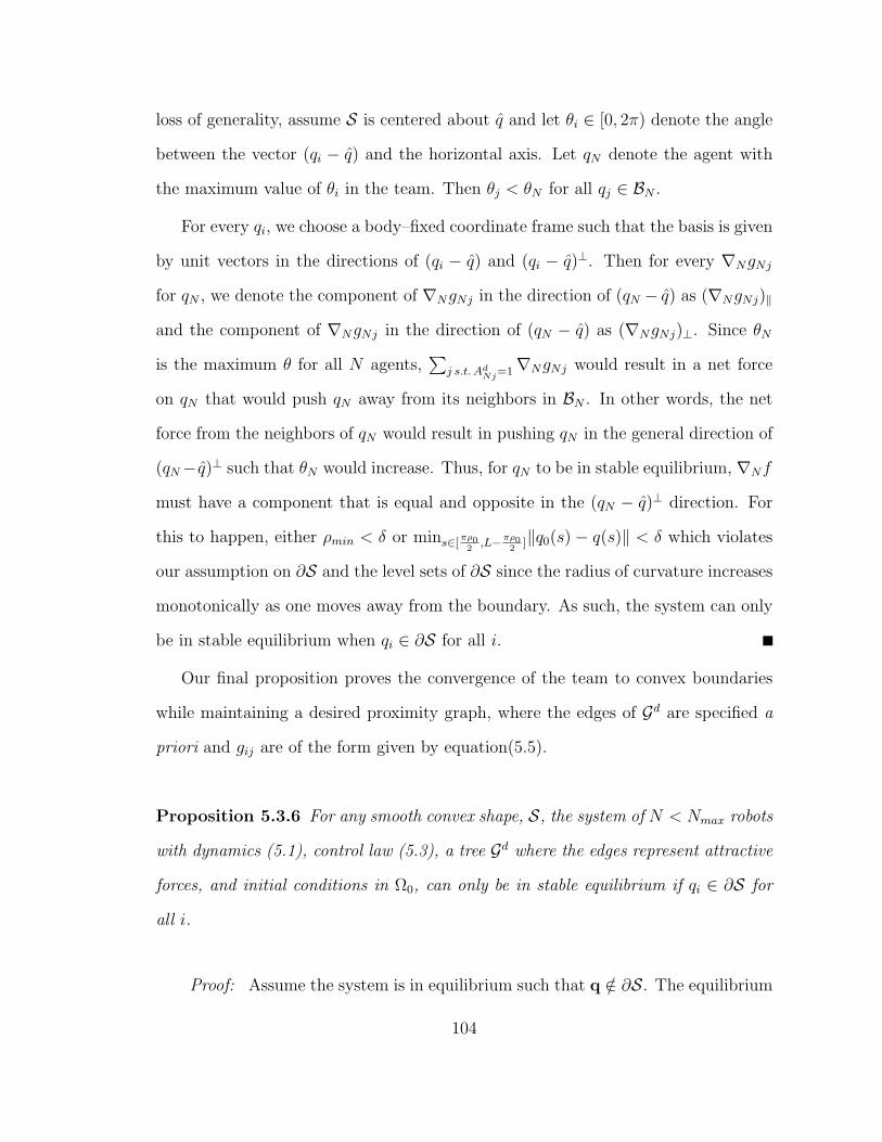
loss of generality, assume S is centered about q and let θi ∈ [0, 2π) denote the angle

between the vector (qi − q) and the horizontal axis. Let qN denote the agent with

the maximum value of θi in the team. Then θj < θN for all qj ∈ BN .

For every qi, we choose a body–fixed coordinate frame such that the basis is given

by unit vectors in the directions of (qi − q) and (qi − q)⊥. Then for every ∇NgNj

for qN , we denote the component of ∇NgNj in the direction of (qN − q) as (∇NgNj)‖

and the component of ∇NgNj in the direction of (qN − q) as (∇NgNj)⊥. Since θN

is the maximum θ for all N agents,∑

j s.t. AdNj=1∇NgNj would result in a net force

on qN that would push qN away from its neighbors in BN . In other words, the net

force from the neighbors of qN would result in pushing qN in the general direction of

(qN− q)⊥ such that θN would increase. Thus, for qN to be in stable equilibrium, ∇Nf

must have a component that is equal and opposite in the (qN − q)⊥ direction. For

this to happen, either ρmin < δ or mins∈[πρ02,L−πρ0

2]‖q0(s) − q(s)‖ < δ which violates

our assumption on ∂S and the level sets of ∂S since the radius of curvature increases

monotonically as one moves away from the boundary. As such, the system can only

be in stable equilibrium when qi ∈ ∂S for all i.

Our final proposition proves the convergence of the team to convex boundaries

while maintaining a desired proximity graph, where the edges of Gd are specified a

priori and gij are of the form given by equation(5.5).

Proposition 5.3.6 For any smooth convex shape, S, the system of N < Nmax robots

with dynamics (5.1), control law (5.3), a tree Gd where the edges represent attractive

forces, and initial conditions in Ω0, can only be in stable equilibrium if qi ∈ ∂S for

all i.

Proof: Assume the system is in equilibrium such that q /∈ ∂S. The equilibrium

104

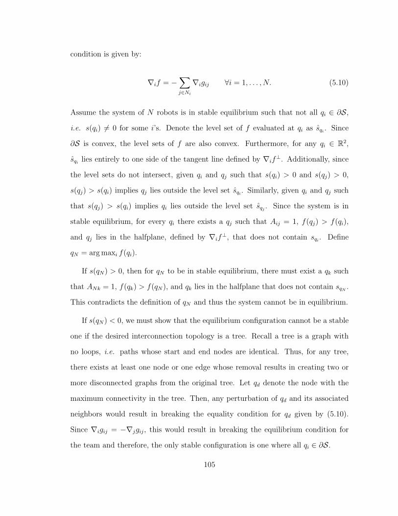
condition is given by:

∇if = −∑j∈Ni

∇igij ∀i = 1, . . . , N. (5.10)

Assume the system of N robots is in stable equilibrium such that not all qi ∈ ∂S,

i.e. s(qi) 6= 0 for some i’s. Denote the level set of f evaluated at qi as sqi . Since

∂S is convex, the level sets of f are also convex. Furthermore, for any qi ∈ R2,

sqi lies entirely to one side of the tangent line defined by ∇if⊥. Additionally, since

the level sets do not intersect, given qi and qj such that s(qi) > 0 and s(qj) > 0,

s(qj) > s(qi) implies qj lies outside the level set sqi . Similarly, given qi and qj such

that s(qj) > s(qi) implies qi lies outside the level set sqj . Since the system is in

stable equilibrium, for every qi there exists a qj such that Aij = 1, f(qj) > f(qi),

and qj lies in the halfplane, defined by ∇if⊥, that does not contain sqi . Define

qN = arg maxi f(qi).

If s(qN) > 0, then for qN to be in stable equilibrium, there must exist a qk such

that ANk = 1, f(qk) > f(qN), and qk lies in the halfplane that does not contain sqN .

This contradicts the definition of qN and thus the system cannot be in equilibrium.

If s(qN) < 0, we must show that the equilibrium configuration cannot be a stable

one if the desired interconnection topology is a tree. Recall a tree is a graph with

no loops, i.e. paths whose start and end nodes are identical. Thus, for any tree,

there exists at least one node or one edge whose removal results in creating two or

more disconnected graphs from the original tree. Let qd denote the node with the

maximum connectivity in the tree. Then, any perturbation of qd and its associated

neighbors would result in breaking the equality condition for qd given by (5.10).

Since ∇igij = −∇jgij, this would result in breaking the equilibrium condition for

the team and therefore, the only stable configuration is one where all qi ∈ ∂S.

105

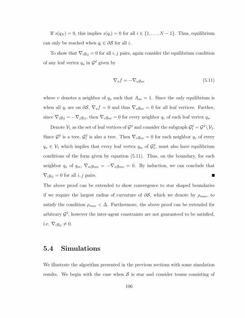
If s(qN) = 0, this implies s(qi) = 0 for all i ∈ 1, . . . , N − 1. Thus, equilibrium

can only be reached when qi ∈ ∂S for all i.

To show that ∇igij = 0 for all i, j pairs, again consider the equilibrium condition

of any leaf vertex qu in Gd given by

∇uf = −∇uguv (5.11)

where v denotes a neighbor of qu such that Auv = 1. Since the only equilibrium is

when all qi are on ∂S, ∇uf = 0 and thus ∇uguv = 0 for all leaf vertices. Further,

since ∇igij = −∇jgij, then ∇vguv = 0 for every neighbor qv of each leaf vertex qu.

Denote V1 as the set of leaf vertices of Gd and consider the subgraph Gd1 = Gd\V1.

Since Gd is a tree, Gd1 is also a tree. Then ∇vguv = 0 for each neighbor qv of every

qu ∈ V1 which implies that every leaf vertex qm of Gd1 , must also have equilibrium

conditions of the form given by equation (5.11). Thus, on the boundary, for each

neighbor qn of qm, ∇mgmn = −∇ngmn = 0. By induction, we can conclude that

∇igij = 0 for all i, j pairs.

The above proof can be extended to show convergence to star shaped boundaries

if we require the largest radius of curvature of ∂S, which we denote by ρmax, to

satisfy the condition ρmax < ∆. Furthermore, the above proof can be extended for

arbitrary Gd, however the inter-agent constraints are not guaranteed to be satisfied,

i.e. ∇igij 6= 0.

5.4 Simulations

We illustrate the algorithm presented in the previous sections with some simulation

results. We begin with the case when S is star and consider teams consisting of

106

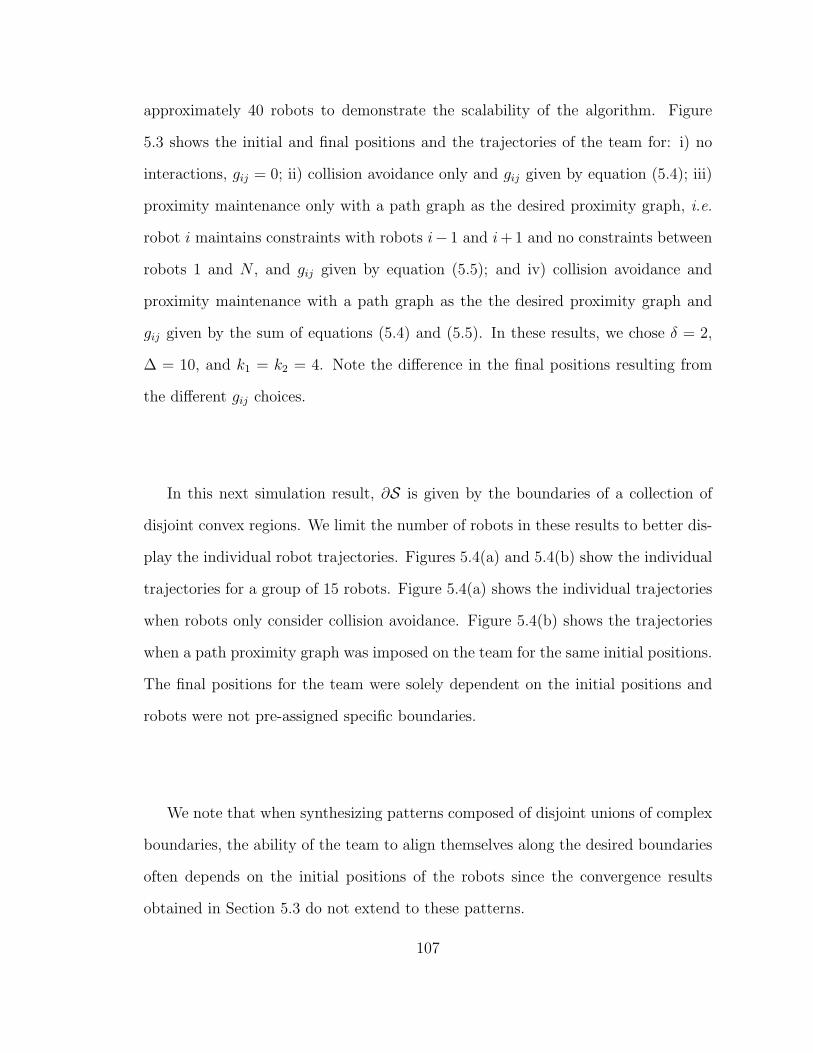
approximately 40 robots to demonstrate the scalability of the algorithm. Figure

5.3 shows the initial and final positions and the trajectories of the team for: i) no

interactions, gij = 0; ii) collision avoidance only and gij given by equation (5.4); iii)

proximity maintenance only with a path graph as the desired proximity graph, i.e.

robot i maintains constraints with robots i− 1 and i+ 1 and no constraints between

robots 1 and N , and gij given by equation (5.5); and iv) collision avoidance and

proximity maintenance with a path graph as the the desired proximity graph and

gij given by the sum of equations (5.4) and (5.5). In these results, we chose δ = 2,

∆ = 10, and k1 = k2 = 4. Note the difference in the final positions resulting from

the different gij choices.

In this next simulation result, ∂S is given by the boundaries of a collection of

disjoint convex regions. We limit the number of robots in these results to better dis-

play the individual robot trajectories. Figures 5.4(a) and 5.4(b) show the individual

trajectories for a group of 15 robots. Figure 5.4(a) shows the individual trajectories

when robots only consider collision avoidance. Figure 5.4(b) shows the trajectories

when a path proximity graph was imposed on the team for the same initial positions.

The final positions for the team were solely dependent on the initial positions and

robots were not pre-assigned specific boundaries.

We note that when synthesizing patterns composed of disjoint unions of complex

boundaries, the ability of the team to align themselves along the desired boundaries

often depends on the initial positions of the robots since the convergence results

obtained in Section 5.3 do not extend to these patterns.

107

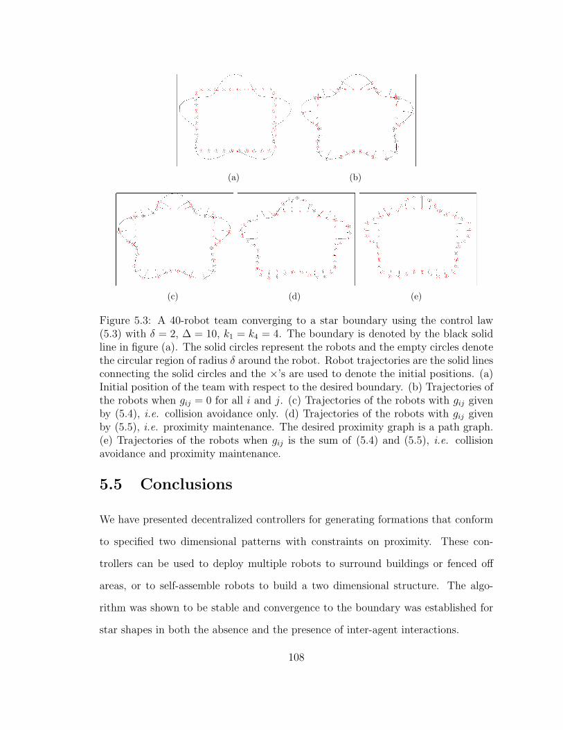
(a) (b)

(c) (d) (e)

Figure 5.3: A 40-robot team converging to a star boundary using the control law(5.3) with δ = 2, ∆ = 10, k1 = k4 = 4. The boundary is denoted by the black solidline in figure (a). The solid circles represent the robots and the empty circles denotethe circular region of radius δ around the robot. Robot trajectories are the solid linesconnecting the solid circles and the ×’s are used to denote the initial positions. (a)Initial position of the team with respect to the desired boundary. (b) Trajectories ofthe robots when gij = 0 for all i and j. (c) Trajectories of the robots with gij givenby (5.4), i.e. collision avoidance only. (d) Trajectories of the robots with gij givenby (5.5), i.e. proximity maintenance. The desired proximity graph is a path graph.(e) Trajectories of the robots when gij is the sum of (5.4) and (5.5), i.e. collisionavoidance and proximity maintenance.

5.5 Conclusions

We have presented decentralized controllers for generating formations that conform

to specified two dimensional patterns with constraints on proximity. These con-

trollers can be used to deploy multiple robots to surround buildings or fenced off

areas, or to self-assemble robots to build a two dimensional structure. The algo-

rithm was shown to be stable and convergence to the boundary was established for

star shapes in both the absence and the presence of inter-agent interactions.

108

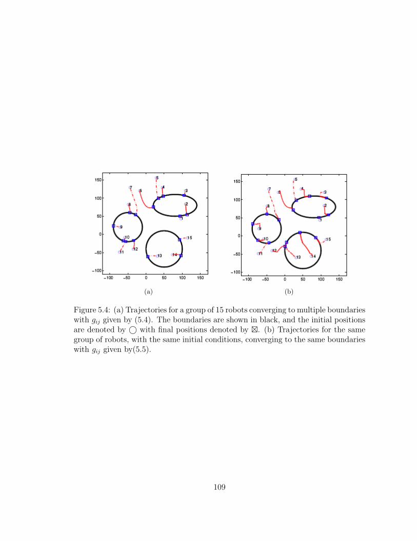
(a) (b)

Figure 5.4: (a) Trajectories for a group of 15 robots converging to multiple boundarieswith gij given by (5.4). The boundaries are shown in black, and the initial positionsare denoted by © with final positions denoted by . (b) Trajectories for the samegroup of robots, with the same initial conditions, converging to the same boundarieswith gij given by(5.5).

109

Chapter 6

Concluding Remarks

Communication in multi–robot research has historically been used to achieve finer

fidelity control and/or perception. While the ubiquity of wireless technology has

enabled us to outfit every robot with the necessary networking tools, it also intro-

duces additional challenges in terms of how best to coordinate the team to maintain

the quality of the communication medium while executing various tasks. This is

mostly due to the difficulty in properly predicting and modeling the radio propaga-

tion mechanisms in the various environments we wish to operate in. This suggests

rather than treating communication solely as a means to improve control and percep-

tion, it is necessary to endow robots with the capability to perceive changes in their

abilities to communicate and respond to them accordingly. As such, the problem of

coordinating multiple autonomous agents to cooperatively achieve a common goal is

inherently a problem at the intersection of communication, control, and perception.

6.1 Contributions

The contributions of this thesis are two fold:

110

Experimentally validated strategies for maintaining communication links

We presented a paradigm and algorithms for the deployment of a team of mobile

robots with strategies for maintaining point-to-point communication links based on

signal strength and/or estimated available bandwidth. First, a methodology is pro-

posed for the automated construction of a radio signal strength map for a partially

known urban environment. We showed how information gleaned from a radio sig-

nal strength map can be used to plan future multi-robot tasks. Coupling this with

low-level reactive controllers that give robots the ability to monitor their commu-

nication links, in particular signal strength measreuments as well as available data

throughput, we can ensure the maintenance of overall network quality during mission

deployment. Experimental results in three representative urban environments were

presented [38,39,41,44].

This work highlights the limitations of the proposed strategies. By design, our

strategies favor constraint satisfaction above reaching goal positions. While such a

strategy allows for real–time status updates from the team and enable the human

operator to deploy additional robots or request a reconfiguration of the whole team

should the original task prove unachievable, the reliance on such contingency strate-

gies may result in serious limitations when deployed in the field. Such considerations

motivated the second contribution of this work: communication–less motion control

strategies.

Provaby correct methods for scalable motion synthesis for teams of robots

Here, we presented two provably correct methods to synthesis communication-less

motion coordination strategies to enable a team of robots to converge onto a desired

boundary curve. First, potential functions, i.e. shape navigation functions, were

synthesized such that all minima within the workspace lie exactly on the desired

111

boundary curve. Decentralized feedback controllers were then derived from these

shape functions to drive the team towards the boundary. These controllers are

decentralized in the sense that agents do not need to communicate each other’s state

information. Rather, we assume each robot is equipped with range and bearing

sensors to enable it to infer neighbors’ relative distance and bearing information.

For our first method, collision avoidance was achieved by modulating each agent’s

descent and orbiting speeds following a local prioritization scheme. Obstacle avoid-

ance was then achieved by introducing a rotational component around the obstacle.

When an obstacle was in close proximity to the boundary, a methodology was pre-

sented to synthesize a new shape navigation function to achieve obstacle avoidance.

In our second method, we extended the shape convergence controller to a system

of particles with second order dynamics. Here, collision avoidance and proximity

maintenance among neighbors were achieved through the use of inter–agent artificial

potential functions.

Both these approaches are efficient and can be used to deploy large robotic teams

to perform perimeter surveillance tasks or to cordon off hazardous areas. Our al-

gorithms are scalable to large number of robots since control inputs rely solely on

local information obtained from each robot’s sensors, thus preserving bandwidth for

critical data transfers. The controllers were shown to be stable and convergence to

the boundary of star shaped sets was established. Lastly, the methodology ensures

that collision and obstacle avoidance are achieved between kinematic robots of finite

size [40, 42,43].

112

6.2 Future Work

There are a few directions for future work that is of particular interest. First we

would like to incorporate some machine learning techniques to the mapping and

exploration of radio signal strength data for a given environment. By incorporating

machine learning with the low-level reactive controllers capable of responding to

changes in signal strength and/or estimated available bandwidth, it may be possible

to concurrently map the propagation characteristics while executing other activities.

Additionally, this may enable the team to find the most optimal configuration for

any given task at all times.

Next, we would like to extend our convergence proofs in the obstacle avoidance

case presented in Chapter 4 to a finite number of obstacles. Furthermore, we would

like to investigate additional topological properties to ensure the proper synthesis

of shape navigation functions when robots fail in close proximity to the desired

boundary. This can in turn provide some ideas for real–time estimation the shape

navigation functions.

Another direction for future work is the extension of the pattern generation con-

troller discussed in Chapter 5 to two dimensional surfaces. This is relevant in ap-

plications such as self-assembly or surface inspection, such as airplanes or ships.

A similar direction is to extend the results in Chapters 4 and 5 to time-varying

boundaries which is relevant in applications like containing oil-spills and monitoring

changing environmental boundaries. Finally, we would like to extend the conver-

gence results discussed in Chapters 4 and 5 to boundaries given by the union of

disjoint convex sets.

In conclusion, we acknowledge the need to implement sensing on individual robots

113

to obtain local state information. It may not be reasonable to expect small, resource-

constrained robots to be able to sense their individual states. However, it is difficult

to get robots to perform tasks like pattern generation in a fixed coordinate frame

without a hardware (or software) solution to the localization problem. The impor-

tant point is that the robots need only local state information and the algorithm is

completely decentralized.

114

Bibliography

[1] Carlos Aguero, Pedro de-las Heras-Quiros, Jose M. Canas, and Vicente Matal-

lan. Pera: Ad-hoc routing protocol for mobile robots. In Proceedings of the

11th International Conference on Advanced Robotics, pages 694–702, Coimbra,

Portugal, July 2003.

[2] O. Albayrak. Line and Circle Formation of Distributed Autonomous Mobile

Robots with Limited Sensor Range. PhD thesis, Naval Postgraduate School,

Monterey, CA, June 1996.

[3] Amarss. Amarss - networked minirhizotron planning and initial deployment.

http://research.cens.ucla.edu/, 2006.

[4] S. O. Anderson, R. Simmons, and D. Goldberg. Maintaining line of sight

communications networks between planetray rovers. In Proceedings of the 2003

IEEE/RSJ Intl. Conference on Intelligent Robots and Systems, pages 2266–

2272, Las Vegas, NV, October 2003.

[5] R. Arkin and J. Diaz. Line-of-sight constrained eploration for reactive multia-

gent robotic teams. In AMC 7th International Workshop on Advanced Motion

Control, 2002.

115

[6] P. Basu and J. Redi. Coordinated flocking of uavs for improved connectivity

of mobile ground nodes. In Proceedings of IEEE MILCOM 2004, 2004.

[7] P. Basu and J. Redi. Movement control algorithms for realization of fault-

tolerant ad-hoc robot networks. IEEE Network, 18(4), July-August 2004.

[8] George Bekey. Autonomous Robots: From Biological Inspiration to Implemen-

tation and Control. MIT Press, 2005.

[9] George Bekey, Robert Ambrose, Vijay Kumar, Art Sanderson, Brian Wilcox,

and Yuan Zheng. Wtec panel report on international assessment of research and

development in robotics. http://www.wtec.org/robotics/, January 2006.

[10] Calin Belta, Guilherme A. S. Pereira, and Vijay Kumar. Abstraction and con-

trol of swarms of robots. In International Symposium of Robotics Research’03,

2003.

[11] A. Bertozzi, Mathieu Kemp, and Daniel Marthaler. Determining environmen-

tal boundaries: Asynchronous communication and physical scales. In Cooper-

ative Control, 2004.

[12] Jon Bredin, Erik Demaine, Mohammad Hajiaghayi, and Daniela Rus. Deploy-

ing sensor nets with guaranteed capacity and fault tolerance. In Proceedings

of Mobihoc 2005, Urbana-Champaign, Illinois, May 2005.

[13] N. F. Britton, N. R. Franks, S. C. Pratt, and T. D. Seeley. Deciding on a new

home: how do honeybees agree? Proc R Soc Lond B, 269, 2002.

[14] L. Chaimowiccz, A. Cowley, D. Gomez-Ibanez, B. Grocholsky, M. A. Hsieh,

H. Hsu, J. F. Keller, V. Kumar, R. Swaminathan, and C. J. Taylor. Deploying

116

air-ground multi-robot teams in urban environments. In Proceedings of the

2005 International Workshop on Multi-Robot Systems, 2005.

[15] L. Chaimowicz, B. Grocholsky, J.F. Keller, V. Kumar, and C.J. Taylor. Ex-

periments in multirobot air-ground coordination. In Proc. IEEE International

Conference on Robotics and Automation, New Orleans, LA, April 2004.

[16] L. Chaimowicz and V. Kumar. Aerial sheperds: Coordination among uavs

and swarms of robots. In Proceedings of the 7th International Symposium on

Distributed Autonomous Robotic Systems (DARS2004), pages 231 – 240, 2004.

[17] L. Chaimowicz, N. Michael, and V. Kumar. Controlling swarms of robots

using interpolated implicit functions. In Proceedings of the 2005 International

Conference on Robotics and Automation (ICRA05), Barcelona, Spain, 2005.

[18] D. E. Chang, S. Shadden, J. E. Marsden, and R. Olfati-Saber. Collision avoid-

ance for multiple agent systems. In Proc. IEEE Conference on Decision and

Control, Maui, Hawaii, 2003.

[19] William Cook. Traveling salesman homepage. http://www.tsp.gatech.edu/.

[20] Peter Corke, Ronald Peterson, and Daniela Rus. Networked robots: Flying

robot navigation using a sensor net. In Proceedings of the Eleventh Interna-

tional Symposium of Robotics Research (ISRR), Springer Tracts on Advanced

Robotics (STAR). Springer-Verlag, October 2003.

[21] T.H. Cormen, C.E. Leiserson, and R.L. Rivest. Introduction to Algorithms.

MIT Press, 1990.

117

[22] Nikolaus Correll and Alcherio Martinoli. System identification of self-

organizing robotic swarms. In Proc. 8th Int. Symp. on Distributed Autonomous

Robotic Systems (DARS) 2006, pages 31–40, Rio de Janeiro, Brazil, 2006.

[23] Nikolaus Correll, Samuel Rutishauser, and Alcherio Martinoli. Comparing co-

ordination schemes for miniature robotic swarms: A case study in boundary

coverage of regular structures. In Proc. 10th International Symposium on Ex-

perimental Robotics (ISER) 2006, Rio de Janeiro, Brazil, 2006.

[24] I. D. Couzin, J. Krause, R. James, G. D. Ruxton, and N. R. Franks. Collective

memory and spatial sorting in animal groups. Journal of Theoretical Biology,

218, 2002.

[25] Jaydev P. Desai, James P. Ostrowski, and Vijay Kumar. Modeling and control

of formations of nonholonomic mobile robots. IEEE Transactions on Robotics

and Automation, 17(6):905–908, 2001.

[26] D. V. Dimarogonas, S. G. Loizou, K. J. Kyriakopoulos, and M. M. Zavlanos.

Decentralized feedback stabilization and collision avoidance of multiple agents.

Technical Report 01-04, NTUA, Athens, Greece, 2004.

[27] Dimos V. Dimarogonas and Kostas J. Kyriakopoulos. A feedback control

scheme for multiple independent dynamic non-point agents. International

Journal of Control, 79(12):1613–1623, December 2006.

[28] Dimos V. Dimarogonas and Kostas J. Kyriakopoulos. Decentralized navigation

functions for multiple robotic agents with limited sensing capabilities. Journal

of Intelligent and Robotic Systems, 48(3):411–433, March 2007.

118

[29] M. P. do Carmo. Differential Geometry of Curves and Surfaces. Prentic-Hall

Inc., 1976.

[30] G. Dudek, M. Jenkin, E. Milios, and D. Wilkes. Experiments in sensing

and communication for robot convoy navigation. In Proceedings of the 2003

IEEE/RSJ Intl. Conference on Intelligent Robots and Systems, pages 268–273,

1995.

[31] Angela Feistel and Slawomir Stanczak. Dynamic resource allocation in wire-

less ad-hoc networks based on QS-CDMA . In The 16th IEEE International

Symposium on Personal, Indoor and Mobile Radio Communications (PIMRC),

Berlin, September 2005. accepted.

[32] R. Fierro, P. Song, A. Das, and V. Kumar. Cooperative control of robot

formations. In R. Murphey and P. Paradalos, editors, Cooperative Control and

Optimization: Series on Applied Optimization, pages 79–93. Kluwer Academic

Press, 2002.

[33] J. Fink, N. Michael, and V. Kumar. Composition of vector fields for multi-

robot manipulation via caging. In Proc. 2007 Robotics: Science and Systems

III, Atlanta, GA, June 2007.

[34] Anita M. Flynn. Gnat robots: a low-intelligence low-cost approach. In Tech-

nical Digest. IEEE Solid-State Sensor and Actuator Workshop, pages 63 – 66,

6-9 June 1988.

[35] B. Grocholsky, S. Bayraktar, V. Kumar, C.J. Taylor, and G. Pappas. Syn-

ergies in feature localization by air-ground robot teams. In 9th International

Symposium on Experimental Robotics (ISER’04), 2004.

119

[36] B. Grocholsky, J. F. Keller, V. Kumar, and G. Pappas. Cooperative air and

ground surveillance: A scalable approach to the detection and localization of

targets by a network of uavs and ugvs. IEEE Robotics & Automation Magazine,

Sept. 2006.

[37] A. Howard, S. Siddiqi, and G. S. Sukhatme. An experimental study of local-

ization using wireless ethernet. In 4th International Conference on Field and

Service Robotics, July 2003.

[38] M. A. Hsieh, A. Cowley, J. F. Keller, L. Chaimowicz, B. Grocholsky, V. Ku-

mar, C. J. Talyor, Y. Endo, R. Arkin, B. Jung, D. Wolf, G. Sukhatme, and

D. C. MacKenzie. Adaptive teams of autonomous aerial and ground robots for

situational awareness. Accepted to the Journal of Field Robotics, To Appear.

[39] M. A. Hsieh, A. Cowley, V. Kumar, and C. J. Taylor. Towards the deployment

of a mobile robot network with end-to-end performance guarantees. In Inter-

national Conference on Robotics and Automation (ICRA) 2006, Orlando, FL,

April 2006.

[40] M. A. Hsieh and V. Kumar. Pattern generation with multiple robots. In

International Conference on Robotics and Automation (ICRA) 2006, Orlando,

FL, April 2006.

[41] M. A. Hsieh, V. Kumar, and C. J. Taylor. Constructing radio signal strength

maps with multiple robots. In Proc. IEEE International Conference on

Robotics and Automation, New Orleans, LA, April 2004.

[42] M. A. Hsieh, S. Loizou, and V. Kumar. Stabilization of multiple robots on

stable orbits via local sensing. In Proceedings of the International Conference

on Robotics and Automation (ICRA) 2007, Rome, Italy, April 2007.

120

[43] M. Ani Hsieh, L. Chaimowicz, and V. Kumar. Decentralized controllers for

shape generation with robotic swarms. Submitted to Robotica, Conditionally

Accepted.

[44] M. Ani Hsieh, A. Cowley, V. Kumar, and C. J. Taylor. Maintaining network

connectivity and performance in robot teams. Accepted to the Journal of Field

Robotics, To Appear.

[45] M. Ani Hsieh, S. Loizou, and V. Kumar. Stabilization of multiple robots on

stable orbits with obstacle avoidance via local sensing. Submitted to Transac-

tions on Robotics, Under Review.

[46] Ali Jadbabaie, J. Lin, and A.S. Morse. Coordination of groups of mobile

autonomous agents using nearest neighbor rules. IEEE Transactions on Auto-

matic Control, July 2003.

[47] M. Jenkin and G. Dudek. The paparazzi problem. In Proc. IEEE/RSJ In-

ternational Conference on Intelligent Robots and Systems (IROS) 2000, pages

2042–2047, Takamatsu, Japan, October 2000.

[48] William Kaiser, Gregory Pottie, Mani Srivastava, Gaurav S. Sukhatme, John

Villasenor, and Deborah Estrin. Networked infomechanical systems (nims) for

ambient intelligence. In Ambient Intelligence, pages 83–114. Springer, 2005.

[49] Shahab Kalantar and Uwe R. Zimmer. Distributed shape control of homoge-

neous swarms of autonomous underwater vehicles. to appear in Autonomous

Robots (intl. journal), 2006.

121

[50] Wesley Kerr and Diana Spears. Robotic simulation of gases for a surveillance

task. In IEEE/RSJ International Conference on Intelligent Robots and Systems

(IROS) 2005, Edmonton, Alberta, Canada, August 2005.

[51] D.E. Koditschek and E. Rimon. Robot navigation functions on manifolds with

boundary. Advances in Applied Math, 11, 1990.

[52] Keith Kotay, Ron Peterson, and Daniela Rus. Experiments with robots and

sensor networks for mapping and navigation. In International Conference on

Field and Service Robotics, Port Douglas, Australia, July 2005.

[53] Naomi Ehrich Leonard and Edward Fiorelli. Virtual leaders, artificial poten-

tials and coordinated control of groups. In Proceedings of the IEEE Interna-

tional Conference on Decision and Control, pages 2968–2973, Orlando, FL,

December 2001.

[54] Magnus Lindhe, Karl Henrik Johansson, and Antonio Bicchi. An experimental

study of exploiting multipath fading for robot communications. In Robotics:

Systems and Science III, Atlanta, GA, June 2007.

[55] S. G. Loizou and K. J. Kyriakopoulos. A feedback based multiagent navigation

framework. International Journal of Systems Science, 2006.

[56] N. Michael, J. Fink, and V. Kumar. Experimental testbed for large teams

of cooperating robots and sensors. IEEE Robotics and Automation Magazine,

2007. Submitted.

[57] Nathan Michael, Calin Belta, and Vijay Kumar. Controlling three dimen-

sional swarms of robots. In IEEE International Conference on Robotics and

Automation (ICRA) 2006, pages 964–969, Orlando, FL, April 2006.

122

[58] Y. Mostofi, T. Chung, R. Murray, and J. Burdick. Communication and sens-

ing trade offs in decentralized mobile sensor networks: A cross-layer design

approach. In 4th International Conference on Information Processing in Sen-

sor Networks (IPSN), Los Angeles, CA, April 2005.

[59] Y. Mostofi and R. Murray. Effect of time-varying fading channels on the control

performance of a mobile sensor node. In Proc. of IEEE 1st International

Conference on Sensor and Ad Hoc Communications and Networks (Secon),

Santa Clara, CA, October 2004.

[60] Benjamin Nabet and Naomi E. Leonard. Shape control of a multi-agent system

using tensegrity structures. In IFAC Workshop on Lagrangian and Hamiltonian

Methods for Nonlinear Control, 2006.

[61] Klara Nahrstedt, Samarth H. Shah, and Kai Chen. Cross-layer architectures

for bandwidth management in wireless networks. In Resource Management in

Wireless Networking, 2004.

[62] A. Neskovic, N. Neskovic, and G. Paunovic. Modern approaches in model-

ing of mobile radio systems propagation environment. IEEE Communications

Surveys, Third Quarter, 2000.

[63] P. Ogren, E. Fiorelli, and N. E. Leonard. Formations with a mission: Stable

coordination of vehicle group maneuvers. In Proc. 15th International Sympo-

sium on Mathematical Theory of Networks and Systems, pages 267–278, Au-

gust 2002.

[64] Reza Olfati-Saber. Flocking for multi-agent dynamic systems: Algorithms and

theory. IEEE Trans. on Automatic Control, 51(3):401–420, March 2006.

123

[65] D. Paley, N. E. Leonard, and R. J. Sepulchre. Collective motion of self-

propelled particles: Stabilizing symmetric formations on closed curves. In

Submitted to 45th IEEE Conference on Decision and Control, San Diego, CA,

2006.

[66] J. K. Parrish, S. V. Viscido, and D. Grunbaum. Self-organized fish schools:

An examination of emergent properties. Biol. Bull., 202, June 2002.

[67] G. A. S. Pereira, A. K. Das, V. Kumar, and M. F. M. Campos. Decentralized

motion planning for multiple robots subject to sensing and communication

constraints. In Proceedings of the Second Multi-Robot Systems Workshop, pages

267–278, Washington, DC, March 2003.

[68] G. A. S. Pereira, V. Kumar, and M. F. M. Campos. Decentralized algorithms

for multi-robot manipulation via caging. The International Journal of Robotics

Research (IJRR), 23(7), July-August 2004.

[69] L. C. A. Pimenta, A. R. Fonseca, G. A. S. Pereira, R. C. Mesquita, E. J. Silva,

W. M. Caminhas, and M. F. M. Campos. On computing complex navigation

functions. In Proc. 2005 Intl. Conf. on Robotics and Automation (ICRA05),

pages 3463–3468, Barcelona, Spain, April 2005.

[70] L. C. A. Pimenta, A. R. Fonseca, G. A. S. Pereira, R. C. Mesquita, E. J.

Silva, W. M. Caminhas, and M. F. M. Campos. Robot navigation based on

electrostatic field computation. IEEE Transactions on Magnetics, 42(4), April

2006.

[71] L. C. A. Pimenta, M. L. Mendes, R. C. Mesquita, and G. A. S. Pereira. Fluids

in electrostatic fields: An analogy for multirobot control. IEEE Transactions

on Magnetics, 43(4), April 2007.

124

[72] Bruno S. Pimentel and Mario F. M. Campos. Cooperative communication in

ad hoc networked mobile robots. In Proceedings of the 2003 IEEE/RSJ Intl.

Conference on Intelligent Robots and Systems, pages 2876–1881, Las Vegas,

NV, October 2003.

[73] M. Powers and T. Balch. Value-based communication preservation for mobile

robots. In 7th International Symposium on Distributed Autonomous Robotic

Systems, 2004.

[74] S. C. Pratt. Quorum sensing by encounter rates in the ant temnothorax al-

bipennis. Behavioral Ecology, 16(2), 2005.

[75] J. Redi, W. Watson, and V. Shurbanov. Energy conserving reception protocols

for ad hoc networks. In Proceedings of MILCOM 2002, October 2002.

[76] C. W. Reynolds. Flocks, herds and schools: A distributed behavioral model.

In Proceedings of the 14th annual conference on Computer Graphics (SIG-

GRAPH’87), pages 25–34. ACM Press, 1987.

[77] E. Rimon and D. E. Koditschek. Exact robot navigation using artificial poten-

tial functions. IEEE Transactions on Robotics and Automation, 8(5):501–518,

October 1992.

[78] Paul E. Rybski, Sascha A. Stoeter, Michael D. Erickson, Maria Gini, Dean F.

Hougen, and Nikolaos Papanikolopoulos. A team of robotic agents for surveil-

lance. In Agents’2000, Barcelona, Spain, June 2000.

[79] R. Sepulchre, D. Paley, and N. E. Leonard. Stabilization of planar collective

motion, part i: All-to-all communication. Accepted for publication in IEEE

Transactions on Automatic Control, 2005.

125

[80] R. Sepulchre, D. Paley, and N. E. Leonard. Stabilization of planar collec-

tive motion with limited communication. Submitted to IEEE Transactions on

Automatic Control, 2006.

[81] P. Song and V. Kumar. A potential field based approach to multi-robot manip-

ulation. In Proc. IEEE Intl. Conf. On Robotics and Automation, Washington,

DC, May 2002.

[82] J. Spletzer and R. Fierro. Optimal positioning strategies for shape changes in

robot teams. In Proceedings of the IEEE International Conference on Robotics

and Automation, pages 754–759, Barcelona, Spain, April 2005.

[83] Gaurav S. Sukhatme, Amit Dhariwal, Bin Zhang, Carl Oberg, Beth Stauf-

fer, and David A. Caron. The design and development of a wireless robotic

networked aquatic microbial observing system. In Environmental Engineering

Science, 2006.

[84] I. Suzuki and M. Yamashita. Distributed anonymous mobile robots: Formation

of geometric patterns. SIAM Journal on Computing, 1999.

[85] J. Sweeney, T. J. Brunette, Y. Yang, and R. A. Grupen. Coordinated teams

of reactive mobile platforms. In Proceedings of the International Conference

on Robotics and Automation (ICRA), pages 99–304, Washington, DC, 2002.

[86] John D. Sweeney, Roderic A. Grupen, and Prashant Shenoy. Active qos flow

maintenance in controlled mobile networks. In Proceedings of the Fourth Inter-

national Symposium on Robotics and Automation (ISRA), Queretaro, Mexico,

August 2004. IEEE.

126

[87] Herbert G. Tanner, Ali Jadbabaie, and George J. Pappas. Flocking in fixed

and switching networks. In Transactions on Automatic Control, 2007.

[88] Herbert G. Tanner and Amit Kumar. Formation Stabilization of Multiple

Agents Using Decentralized Navigation Functions. MIT Press, 2005.

[89] BBN Technologies. BBN JBox Informal Manual. BBN Technologies, 2003.

[90] B. J. Thibodeau, A. H. Fagg, and B. N. Levine. Signal strength coordination

for cooperative mapping. Technical report, Department of Computer Science,

University of Massachusetts, Amherst, 2004.

[91] Massayoshi Tomizuka. Advanced vehicle control systems (avcs) research for

automated highway systems in california path. In Proceedings of the IEEE

Vehicle Navigation and Information Systems Conference, pages PLEN41 – 45,

31 Aug.-2 Sept. 1994.

[92] T. Vicsek, A. Czirok, E. Ben-Jacob, I. Cohen, and O. Shochet. Novel type of

phase transition in a system of self-driven particles. Physical Review Letters,

75(6):1226–9, 1995.

[93] A. R. Wagner and R. C. Arkin. Communication-sensitive multi-robot recon-

naissance. In Proceedings of the IEEE International Conference on Robotics

and Automation (ICRA), pages 2480–2487, 2004.

[94] Wikipedia. Asimov. en.wikipedia.org/wiki/Asimov.

[95] Wikipedia. Nikola tesla. en.wikipedia.org/wiki/Nikola_Tesla.

[96] Wikipedia. Remote control. en.wikipedia.org/wiki/Remote_control.

[97] Wikipedia. Robot. en.wikipedia.org/wiki/Robot.

127

[98] A. F. T. Winfield. Distributed sensing and data collection via broken ad hoc

wireless connected network of mobile robots. In G. Bekey L. E. Parker and

J. Barhen, editors, Distributed Autonomous Robotic Systems 4, pages 273–282.

Springer-Verlag, 2000.

[99] Yuan Xue and Klara Nahrstedt. Providing fault-tolerant ad-hoc routing service

in adversarial environments. Wireless Personal Communications, Special Issue

on Security for Next Generation Communications, 2004.

[100] Bin Zhang and Gaurav S. Sukhatme. Controlling sensor density using mobility.

In The Second IEEE Workshop on Embedded Networked Sensors, pages 141 –

149, May 2005.

[101] F. Zhang, D. M. Fratantoni, D. Paley, J. Lund, and N. E. Leonard. Control

of coordinated patterns for ocean sampling. International Journal of Control,

80(7):1186–1199, 2007.

[102] F. Zhang, M. Goldgeier, and P. S. Krishnaprasad. Control of small formations

using shape coordinates. In Proc. of 2003 International Conf. of Robotics and

Automation, pages 2510–2515, Taipei, Taiwan, 2003. IEEE.

[103] F. Zhang and N. E. Leonard. Coordinated patterns of unit speed particles on

a closed curve. Systems and Control Letters (submitted), 2006.

[104] F. Zhang and N. E. Leonard. Coordinated patterns of unit speed particles on

a closed curve. Systems and Control Letters, 56(6):397–407, 2007.

128