Monopoly and monopoly behavior Alexandre Mateus Sara Levy Tiago Ratinho

Welcome message from author
This document is posted to help you gain knowledge. Please leave a comment to let me know what you think about it! Share it to your friends and learn new things together.
Transcript
Monopolyand monopoly behavior
Alexandre MateusSara Levy
Tiago Ratinho
2
Monopoly
• We’ve seen the behaviour of a competitive industry, a market structure characterised by a great number of small firms
• Now, we consider the opposite extreme and study the behaviour of a market structure with only one firm in the industry MONOPOLY
• The level of price is chosen in order to maximize its profits
• The monopolist can choose the price and let the consumers pick the quantity or it can choose the quantity and see what price the consumers wish to pay for it.
3
Maximizing Profits
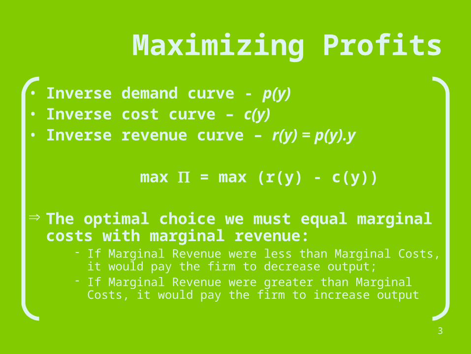
• Inverse demand curve - p(y)• Inverse cost curve – c(y)• Inverse revenue curve – r(y) = p(y).y
max = max (r(y) - c(y))
The optimal choice we must equal marginal costs with marginal revenue:
If Marginal Revenue were less than Marginal Costs, it would pay the firm to decrease output;
If Marginal Revenue were greater than Marginal Costs, it would pay the firm to increase output
4
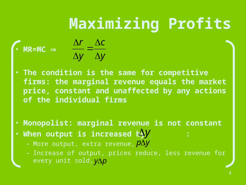
• MR=MC
• The condition is the same for competitive firms: the marginal revenue equals the market price, constant and unaffected by any actions of the individual firms
• Monopolist: marginal revenue is not constant• When output is increased by :
– More output, extra revenue,– Increase of output, prices reduce, less revenue for every
unit sold,
Maximizing Profits
y
c
y
r
y
py
py
5
Maximizing Profits
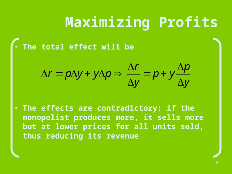
• The total effect will be
• The effects are contradictory: if the monopolist produces more, it sells more but at lower prices for all units sold, thus reducing its revenue
y
pyp
y
rpyypr
6
Maximizing Profits
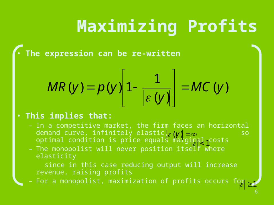
• The expression can be re-written
• This implies that:– In a competitive market, the firm faces an horizontal
demand curve, infinitely elastic, so optimal condition is price equals marginal costs
– The monopolist will never position itself where elasticity since in this case reducing output will increase revenue,
raising profits– For a monopolist, maximization of profits occurs for
)()(
11)()( yMC
yypyMR
)(y1
1
7
Linear Demand Curve and Monopoly
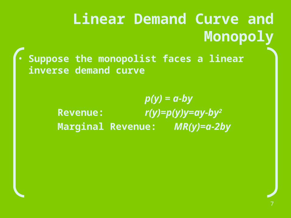
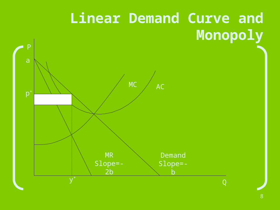
• Suppose the monopolist faces a linear inverse demand curve
p(y) = a-byRevenue: r(y)=p(y)y=ay-by2
Marginal Revenue: MR(y)=a-2by
8
Linear Demand Curve and Monopoly
Q
P
DemandSlope=-b
MRSlope=-2b
a
MC ACp*
y*
9
Markup Pricing
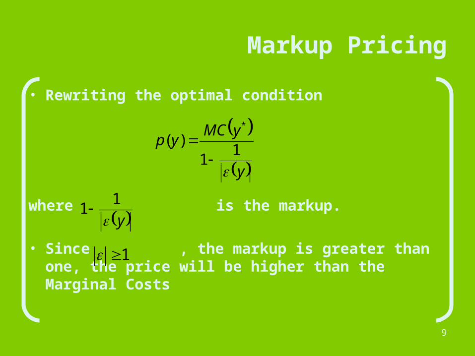
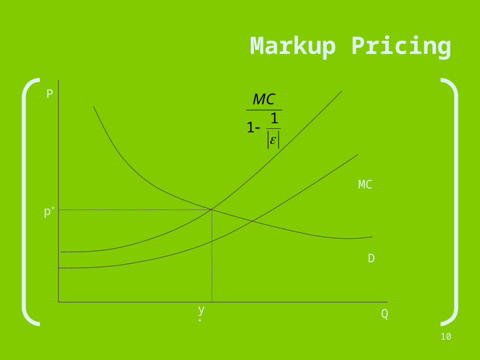
• Rewriting the optimal condition
where is the markup.
• Since , the markup is greater than one, the price will be higher than the Marginal Costs
y
yMCyp
1
1)(
*
y1
1
1
10
Markup Pricing
Q
P
p*
y*
D
MC
1
1
MC
11
The Impact of Taxes on a Monopolist
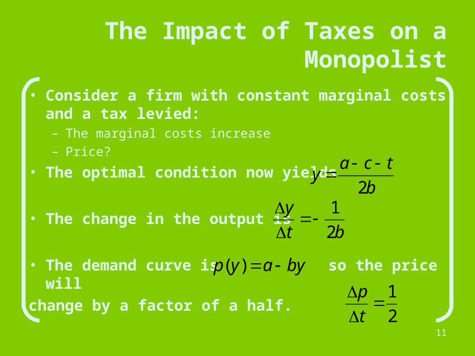
• Consider a firm with constant marginal costs and a tax levied:– The marginal costs increase– Price?
• The optimal condition now yields
• The change in the output is
• The demand curve is so the price will
change by a factor of a half.
b
tcay
2
bt
y
2
1
byayp )(
2
1
t
p
12
The Impact of Taxes on a Monopolist
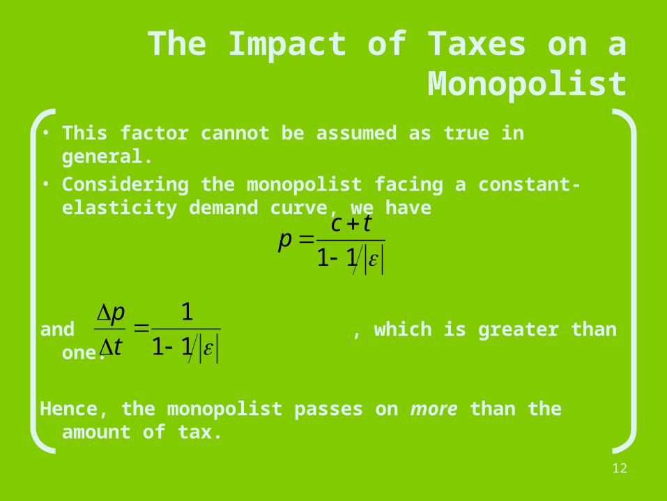
• This factor cannot be assumed as true in general.
• Considering the monopolist facing a constant-elasticity demand curve, we have
and , which is greater than one.
Hence, the monopolist passes on more than the amount of tax.
11
tc
p
11
1
t
p
13
The Impact of Taxes on a Monopolist
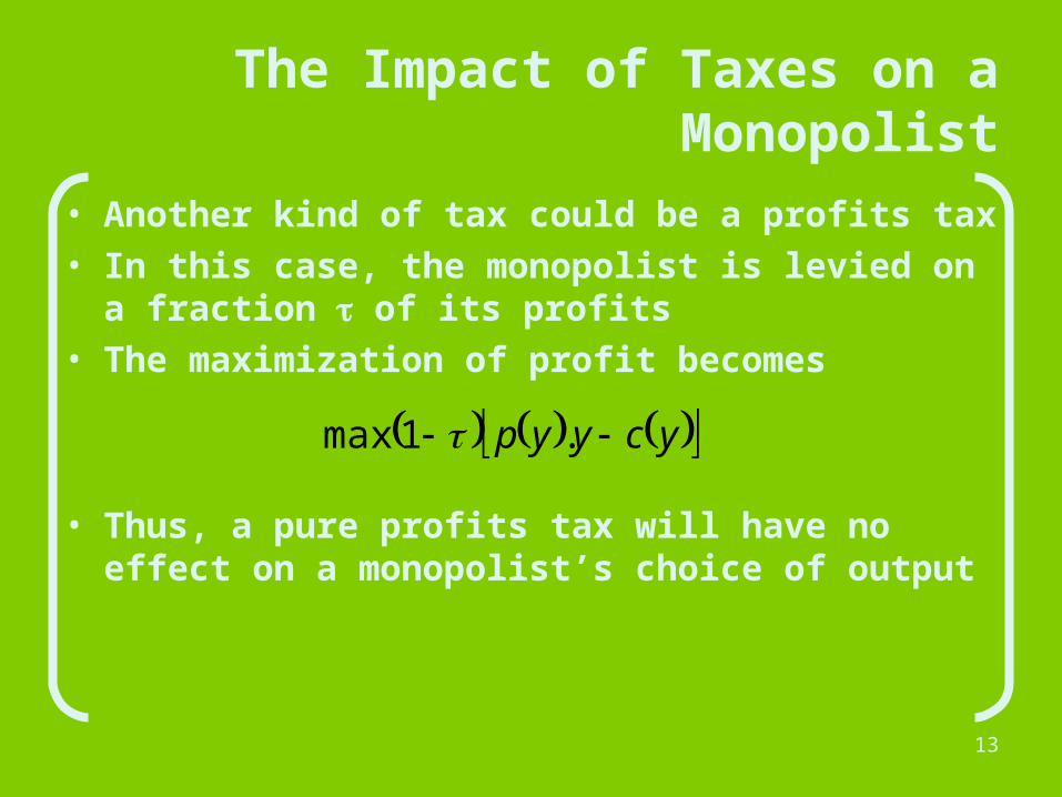
• Another kind of tax could be a profits tax• In this case, the monopolist is levied on a
fraction of its profits• The maximization of profit becomes
• Thus, a pure profits tax will have no effect on a monopolist’s choice of output
ycyyp .1max
14
Inefficiency of Monopoly
• The monopolist operates with prices greater than Marginal Costs prices higher and output lower than in a competitive environment consumers typically be worse
• In contrast, firms will be better under monopoly, as they can manipulate the price in order to increased profits
• An economic arrangement is Pareto efficient if there is no way to make anyone better without making anyone worse, so
Is the monopoly Pareto Efficient?
15
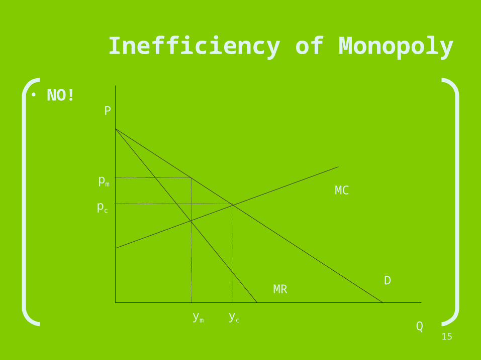
Inefficiency of Monopoly
• NO!
Q
P
ym yc
MC
DMR
pc
pm
16
Inefficiency of Monopoly
• Since p > Marginal Costs extra output could be sold at a price lower than the market price, but still higher than MC each side gets better
• The monopoly is not Pareto efficient because the monopolist cannot lower the price of the extra units without lowering the prices of all units
17
Deadweight Loss of the Economy
• Measure how inefficient is a monopoly variations of producers’ and consumers’ surpluses by imposing a perfect competition to a monopoly situation
18
Deadweight Loss of the Economy
Q
P
y*
MC
pc
p*
MRD
AB
C
19
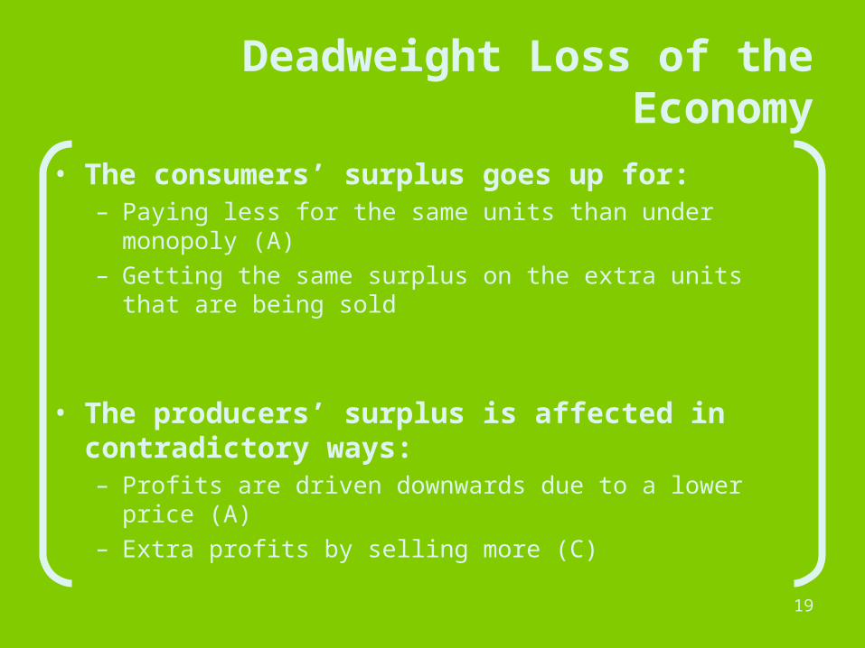
Deadweight Loss of the Economy
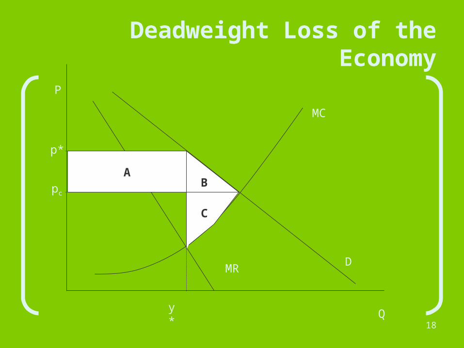
• The consumers’ surplus goes up for:– Paying less for the same units than under monopoly (A)– Getting the same surplus on the extra units that are
being sold
• The producers’ surplus is affected in contradictory ways:– Profits are driven downwards due to a lower price (A)– Extra profits by selling more (C)
20
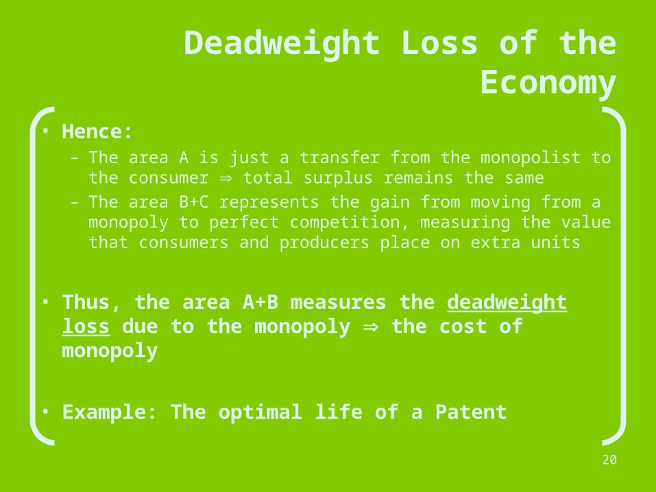
Deadweight Loss of the Economy
• Hence:– The area A is just a transfer from the monopolist to the
consumer total surplus remains the same– The area B+C represents the gain from moving from a
monopoly to perfect competition, measuring the value that consumers and producers place on extra units
• Thus, the area A+B measures the deadweight loss due to the monopoly the cost of monopoly
• Example: The optimal life of a Patent

Natural Monopoly
22
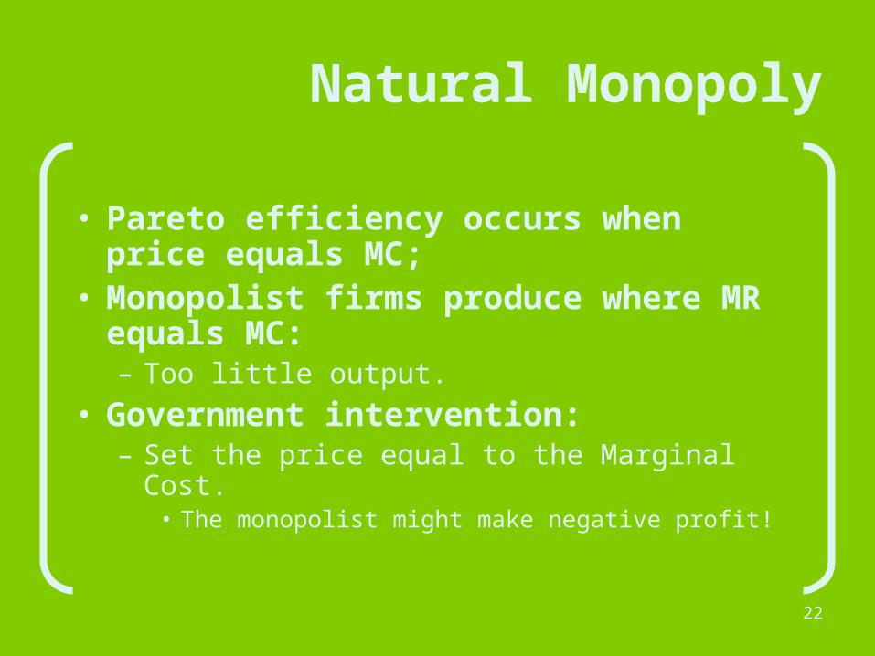
Natural Monopoly
• Pareto efficiency occurs when price equals MC;
• Monopolist firms produce where MR equals MC: – Too little output.
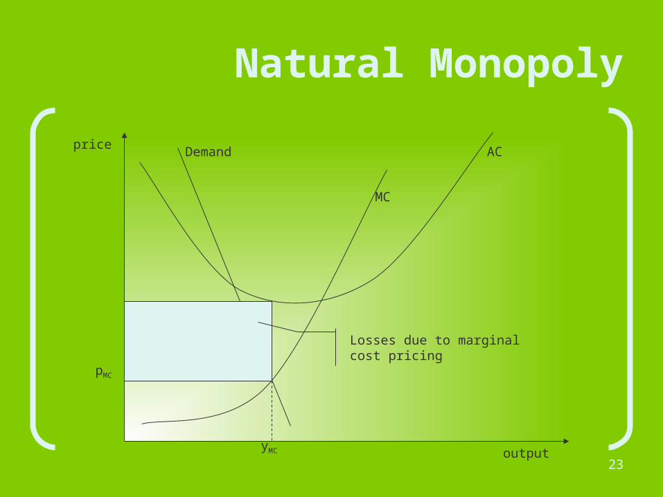
• Government intervention:– Set the price equal to the Marginal Cost.
• The monopolist might make negative profit!
23output
price
MC
ACDemand
yMC
pMC
Natural Monopoly
Losses due to marginal cost pricing
24
Natural Monopoly
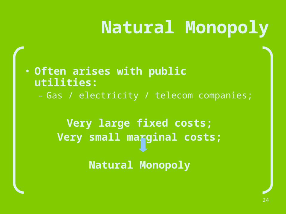
• Often arises with public utilities:– Gas / electricity / telecom companies;
Very large fixed costs;Very small marginal costs;
Natural Monopoly
25
Problem
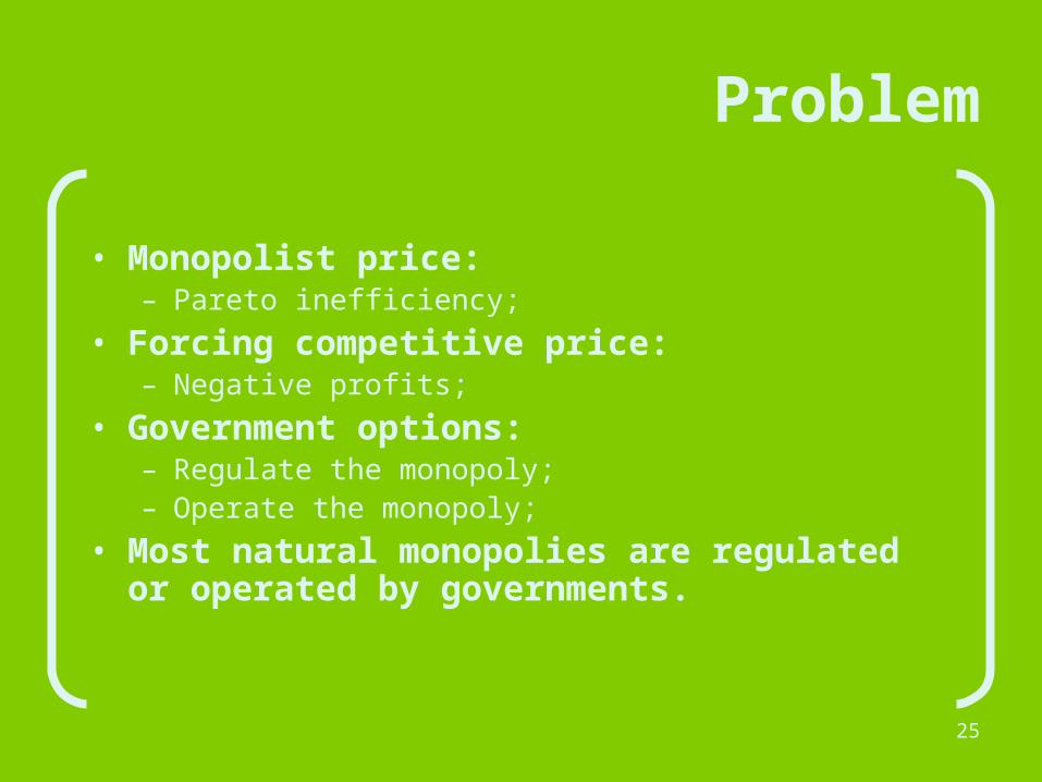
• Monopolist price:– Pareto inefficiency;
• Forcing competitive price:– Negative profits;
• Government options:– Regulate the monopoly;– Operate the monopoly;
• Most natural monopolies are regulated or operated by governments.
26
Government regulation
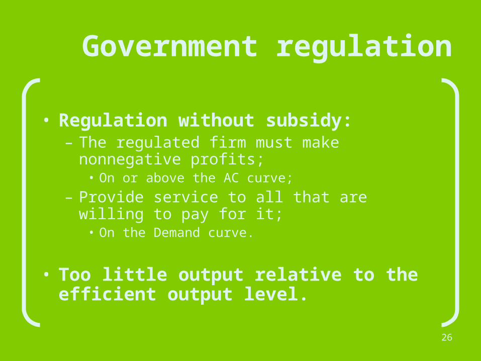
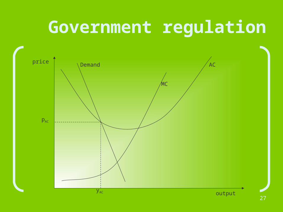
• Regulation without subsidy:– The regulated firm must make
nonnegative profits;• On or above the AC curve;
– Provide service to all that are willing to pay for it;
• On the Demand curve.
• Too little output relative to the efficient output level.
27output
price
MC
ACDemand
yAC
pAC
Government regulation
28
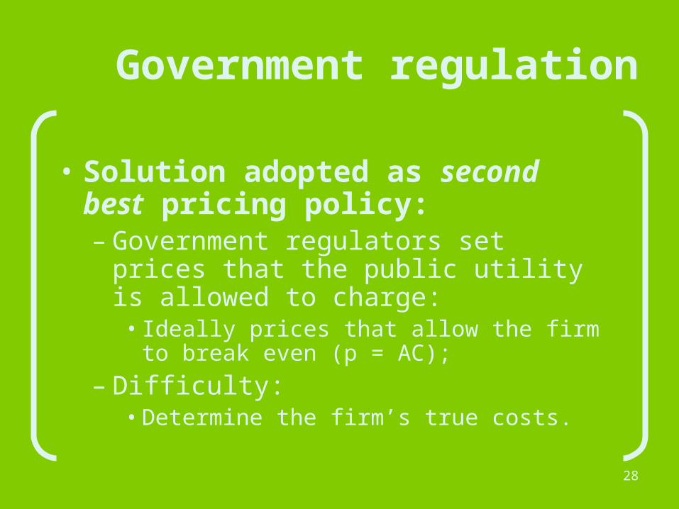
Government regulation
• Solution adopted as second best pricing policy:– Government regulators set prices
that the public utility is allowed to charge:• Ideally prices that allow the firm to
break even (p = AC);
– Difficulty:• Determine the firm’s true costs.

29
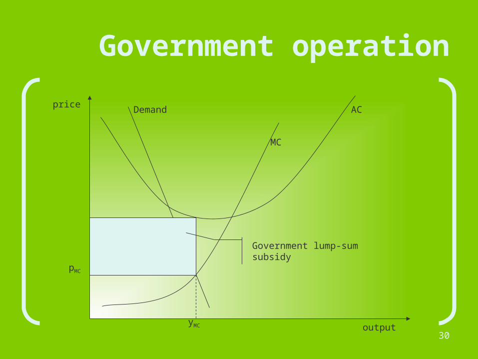
Government operation
• Operate at the point where the price equals the marginal costs (p=MC);
• Provide a lump-sum subsidy to keep the firm in operation.
• Difficulty:– Determine the firm’s true costs;
30output
price
MC
ACDemand
yMC
pMC
Government operation
Government lump-sum subsidy
What causes monopolies?
32
What causes monopolies?
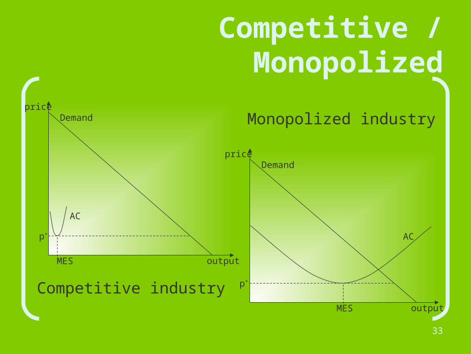
• When is an industry competitive and when is it monopolized?– In general it depends on the relationship
between the Demand and the Average Cost curves;
– Crucial factor:• Size of the Minimum Efficient Scale (MES)
relative to the size of demand. MES = level of output that minimizes average cost
33
Competitive / Monopolized
output
priceDemand
AC
MES
p*
Competitive industryoutput
priceDemand
AC
MES
p*
Monopolized industry
34
Competitive / Monopolized
• Average Cost curve:– Shape determined by the underlying
technology;• Important to determine if the industry is
competitive or monopolized:– Relation between the MES and the size of the
market;
• Economic policy:– Can influence the size of the market;
35
Other reasons
• Cartel:– Different firms in the same industry collude;
• Restrict output;• Raise prices;• Generate more profit;
– Illegal!
• Historical accident:– One large firm that entered the market first;– Cost advantage to discourage other firms to
enter the market.

Monopoly behavior
37
Introduction
• Competitive market:– A firm raises the price above the market price:
• Costumers desert it in favor of its competitors;
• Monopolized market:– Monopolist firm raises the price:
• Looses some customers, but not all.
• Most firms stand somewhere between these extremes.
• Firm with some degree of monopoly has more options:– More complex pricing and marketing strategies;– Some degree of differentiation.
Price discrimination
39
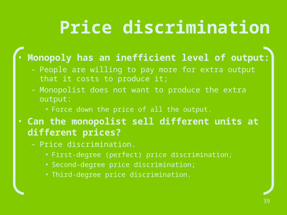
Price discrimination
• Monopoly has an inefficient level of output:– People are willing to pay more for extra output that it
costs to produce it;– Monopolist does not want to produce the extra output:
• Force down the price of all the output.
• Can the monopolist sell different units at different prices?– Price discrimination.
• First-degree (perfect) price discrimination;• Second-degree price discrimination;• Third-degree price discrimination.
First-degree price discrimination
41
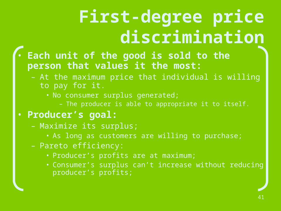
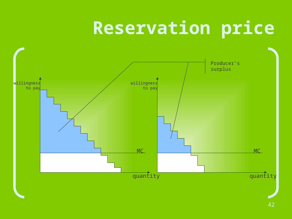
First-degree price discrimination
• Each unit of the good is sold to the person that values it the most:– At the maximum price that individual is willing to pay for
it.• No consumer surplus generated;
– The producer is able to appropriate it to itself.
• Producer’s goal:– Maximize its surplus;
• As long as customers are willing to purchase;– Pareto efficiency:
• Producer’s profits are at maximum;• Consumer’s surplus can’t increase without reducing
producer’s profits;
42
quantity
willingnessto pay
MC
quantity
willingnessto pay
MC
Reservation price
Producer’s surplus
43
Perfect price discriminator producer
• Produces at an output level where price equals Marginal Cost;– Price MC
• someone willing to pay more for an extra unit than it costs to produce it;
– Price < MC • Negative profit;
44
Different perspective
• So far:– “selling each unit as the maximum price
someone is willing to pay for it”
• Another perspective:– Selling a fixed amount of the good at a
“take it or leave it” price.
45
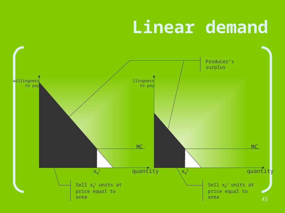
Linear demand
quantity
willingnessto pay
MC
x02quantity
willingnessto pay
MC
x01
Producer’s surplus
Sell x01 units at price
equal to areaSell x0
2 units at price equal to area
Second degree price discrimination
47
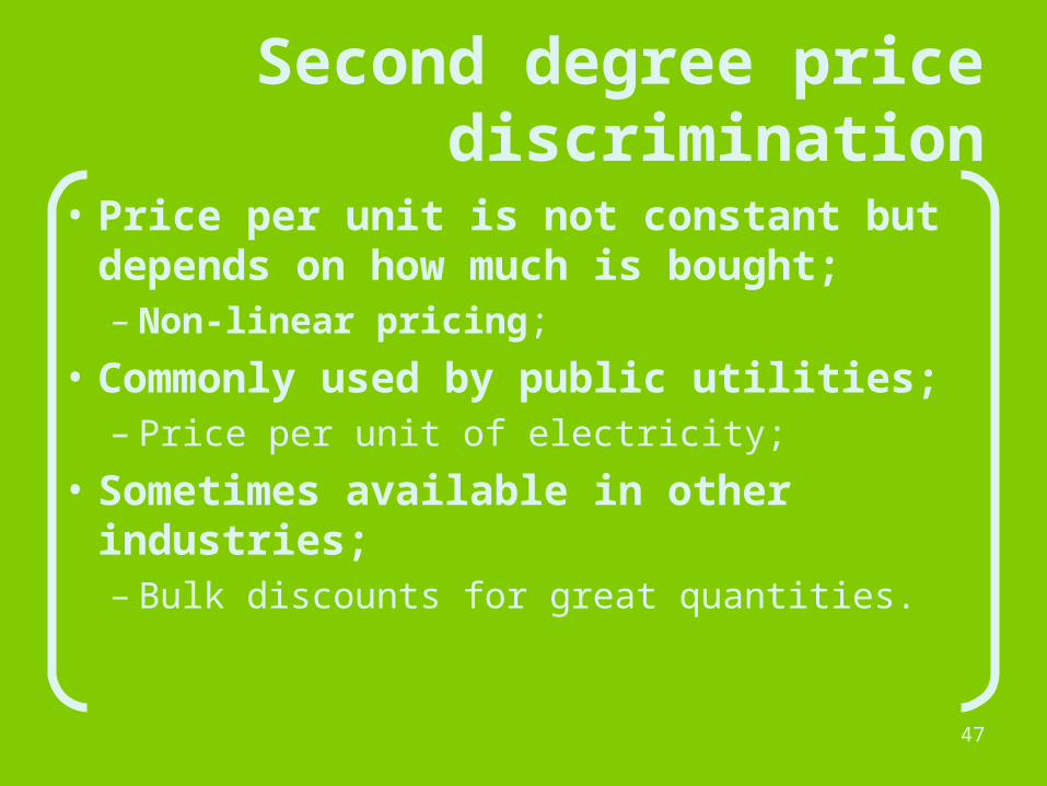
Second degree price discrimination
• Price per unit is not constant but depends on how much is bought;– Non-linear pricing;
• Commonly used by public utilities;– Price per unit of electricity;
• Sometimes available in other industries;– Bulk discounts for great quantities.
48
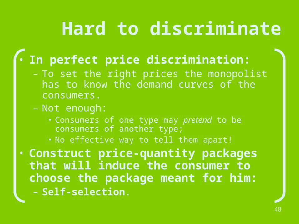
Hard to discriminate
• In perfect price discrimination:– To set the right prices the monopolist has to
know the demand curves of the consumers.– Not enough:
• Consumers of one type may pretend to be consumers of another type;
• No effective way to tell them apart!
• Construct price-quantity packages that will induce the consumer to choose the package meant for him:– Self-selection.
49
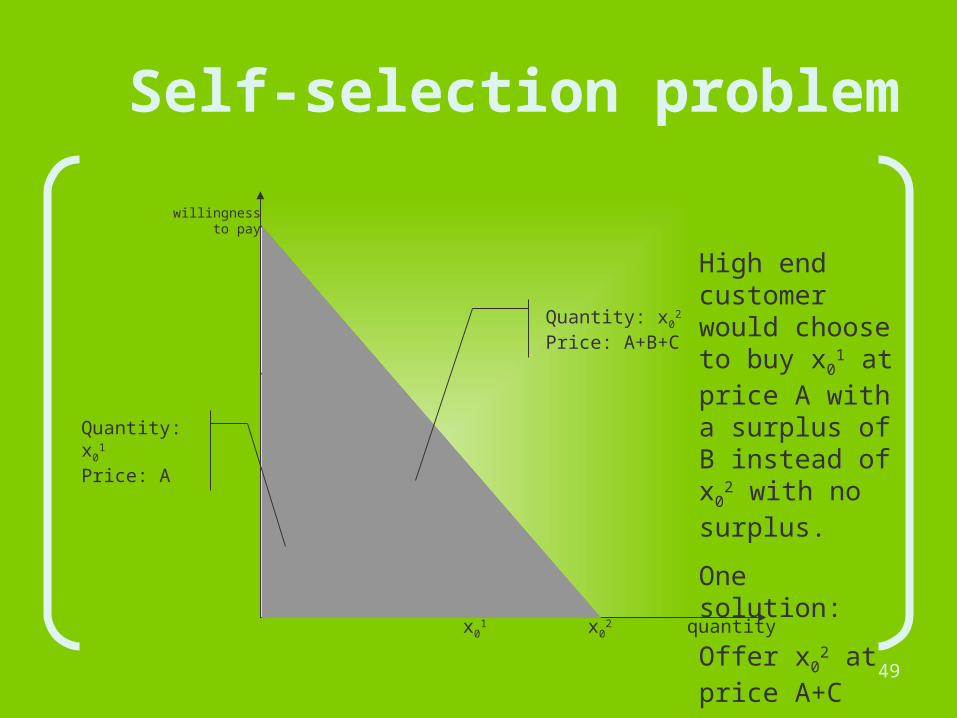
Self-selection problem
quantity
willingnessto pay
x01
A
C
B
x02
Quantity: x02
Price: A+B+C
Quantity: x01
Price: A
High end customer would choose to buy x0
1 at price A with a surplus of B instead of x0
2 with no surplus.
One solution:
Offer x02 at price
A+C
50
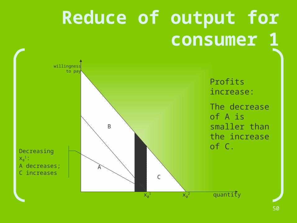
Reduce of output for consumer 1
quantity
willingnessto pay
x01
A
C
B
x02
Decreasing x01:
A decreases;C increases
Profits increase:
The decrease of A is smaller than the increase of C.
51
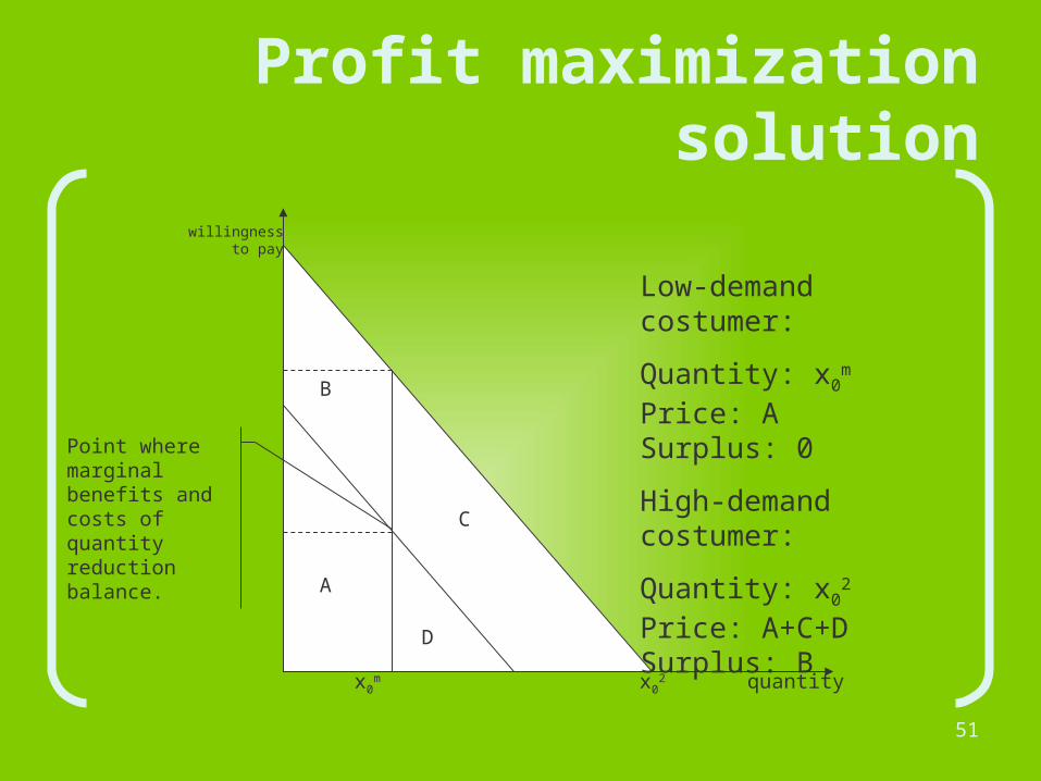
Profit maximization solution
quantity
willingnessto pay
x0m
A
C
B
x02
D
Point where marginal benefits and costs of quantity reduction balance.
Low-demand costumer:
Quantity: x0m
Price: ASurplus: 0
High-demand costumer:
Quantity: x02
Price: A+C+DSurplus: B
52
In practice
• Self-selection encouraged by adjusting the quality of the good instead of its quantity.
• Example:– Airline companies:
• Business tickets:– No restrictions;
• Other tickets:– Stay over Saturday night, buy 14 days in advance, etc;
– Business travelers are willing to pay for business tickets;– Tourists consider the restrictions acceptable;– Company profits more than by selling tickets at a flat
price.

Third degree price discrimination
54
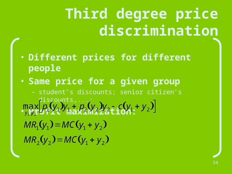
Third degree price discrimination
• Different prices for different people• Same price for a given group
– student’s discounts; senior citizen’s discounts,...;
• Profit maximization:
55
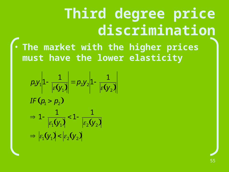
Third degree price discrimination
• The market with the higher prices must have the lower elasticity
p1y111
y1 p2y21
1
y2 IF p1 p2
1 1
1 y1 1 1
2 y2 1 y1 2 y2
56
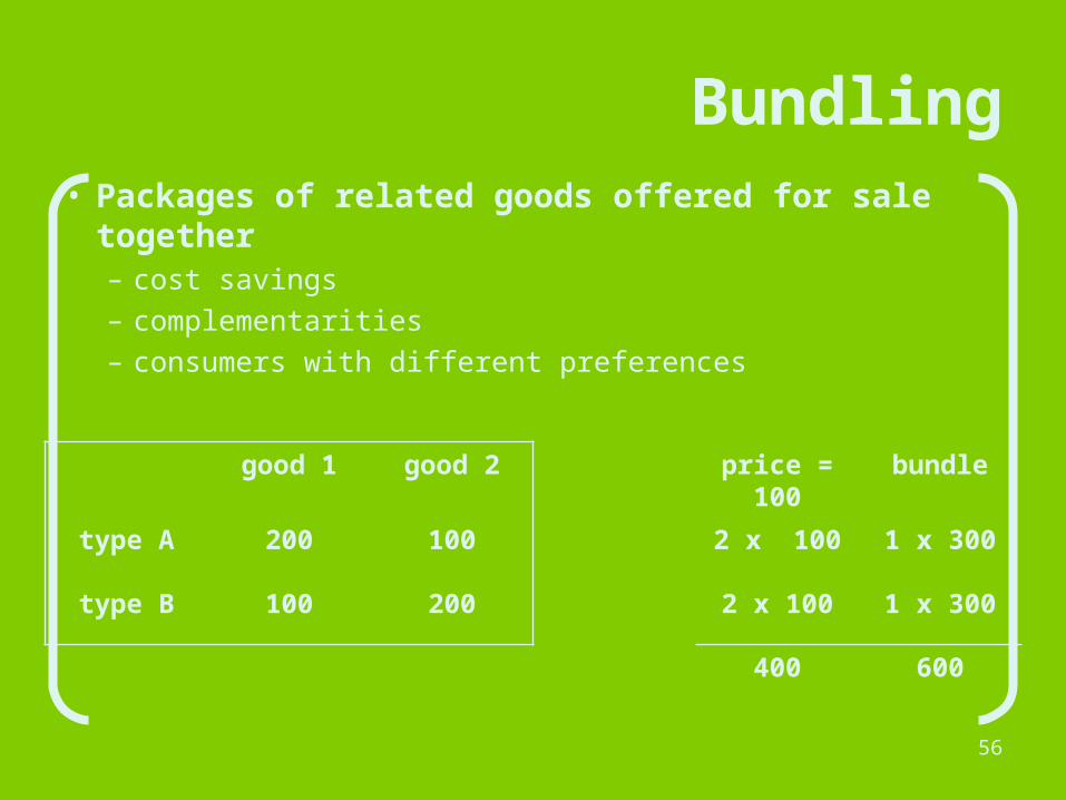
Bundling• Packages of related goods offered for sale
together– cost savings – complementarities– consumers with different preferences
good 1 good 2 price = 100
bundle
type A 200 100 2 x 100 1 x 300
type B 100 200 2 x 100 1 x 300
400 600
57
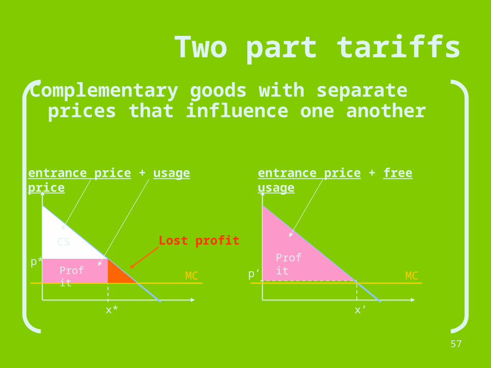
Two part tariffsComplementary goods with separate
prices that influence one another
p*
x*
MC
CS Lost profit
Profit p’
x’
MC
Profit
entrance price + usage price entrance price + free usage
58
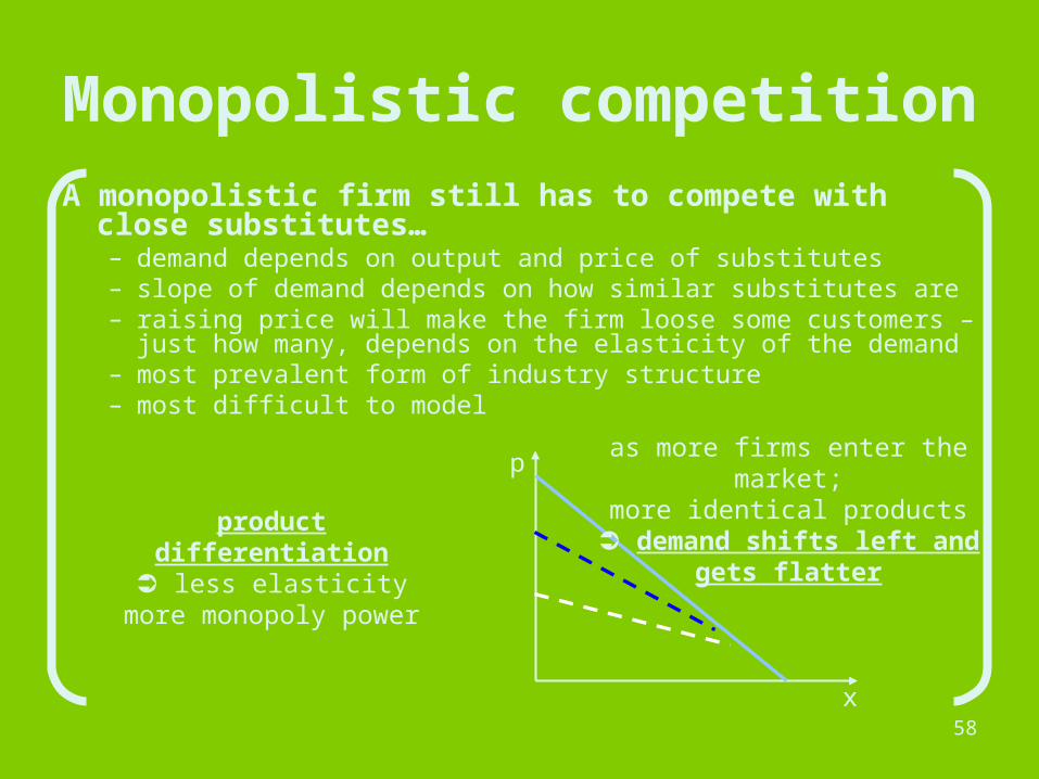
Monopolistic competitionA monopolistic firm still has to compete with
close substitutes…– demand depends on output and price of substitutes – slope of demand depends on how similar substitutes are– raising price will make the firm loose some customers – just
how many, depends on the elasticity of the demand– most prevalent form of industry structure– most difficult to model
product differentiation➲ less elasticity
more monopoly power
p
x
as more firms enter the market;more identical products
➲ demand shifts left andgets flatter
59
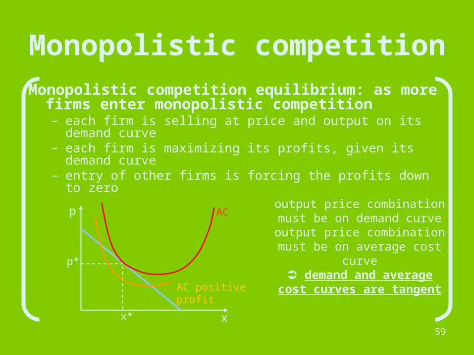
Monopolistic competitionMonopolistic competition equilibrium: as more
firms enter monopolistic competition– each firm is selling at price and output on its demand
curve– each firm is maximizing its profits, given its demand
curve– entry of other firms is forcing the profits down to zero
p
x
output price combination must be on demand curve
output price combination must be on average cost curve
➲ demand and average cost curves are tangent
AC
p*
x*
AC positive profit
60
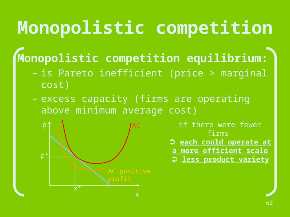
Monopolistic competition
Monopolistic competition equilibrium: – is Pareto inefficient (price > marginal cost)– excess capacity (firms are operating above
minimum average cost)
p
x
if there were fewer firms ➲ each could operate at a
more efficient scale➲ less product variety
AC
p*
x*
AC positive profit

61
Product differentiation
Monopolistic competition equilibrium: – doesn’t promote product differentiation– example of ice-cream vendors
– vendors tend to move close to each other in order to ”steal” the other’s market share without loosing their own customers
Related Documents