Modeling Propeller Aerodynamics and Slipstream Effects on ...Modeling Propeller Aerodynamics and Slipstream Effects on Small UAVs in Realtime Michael S. Selig∗ University of Illinois

AIAA Atmospheric Flight Mechanics 2010 Conference 2010-7938 2-5 Aug 2010, Toronto, Ontario, Canada

Copyright © 2010 by the author. Published by the American Institute of Aeronautics and Astronautics, Inc., with permission.

Modeling Propeller Aerodynamics and Slipstream

Effects on Small UAVs in Realtime

Michael S. Selig∗

University of Illinois at Urbana-Champaign, Urbana, IL 61801, USA

This paper focuses on strong propeller effects in a full six degree-of-freedom (6-DOF) aerodynamic modeling of small UAVs at high angles of attack and high sideslipin maneuvers performed using large control surfaces at large deflections for aircraftwith high thrust-to-weight ratios. For such configurations, the flight dynamics can bedominated by relatively large propeller forces and strong propeller slipstream effectson the downstream surfaces, e.g., wing, fuselage and tail. Specifically, the propellerslipstream effects include propeller wash flow speed effects, propeller wash lag inspeed and direction, flow shadow effects and several more that are key to capturingflight dynamics behaviors that are observed to be common to high thrust-to-weightratio aircraft. The overall method relies on a component-based approach, whichis discussed in a companion paper, and forms the foundation of the aerodynamicsmodel used in the RC flight simulator FS One. Piloted flight simulation results for asmall RC/UAV configuration having a wingspan of 1765 mm (69.5 in) are presentedhere to highlight results of the high-angle propeller/aircraft aerodynamics modelingapproach. Maneuvers simulated include knife-edge power-on spins, upright power-onspins, inverted power-on pirouettes, hovering maneuvers, and rapid pitch maneuversall assisted by strong propeller-force and propeller-wash effects. For each case, theflight trajectory is presented together with time histories of aircraft state data duringthe maneuvers, which are discussed.

Nomenclature

A = propeller disc areaa = airfoil lift curve slope (2π)CQ = propeller torque coefficient (Q/ρn2D5)CT = propeller thrust coefficient (T/ρn2D4)D = propeller diameterI = mass moment of inertiaJ = propeller advance ratio based on VN

k = constant, semi-empirical correction coefficientM = pitching moment about y-axis (positive nose up)m = jet flow parameter (V∞N/Vdisc,N )mj = mass flow rateN = yawing moment about z-axis (positive nose right)n = propeller rotational speed (revs/sec)Nj = propeller normal force due to angle of attack (method 2)NP = propeller yawing moment due to angle of attackp, q, r = body-axis roll, pitch and yaw rate

∗Associate Professor, Department of Aerospace Engineering, 104 S. Wright St. Senior Member AIAA.http://www.ae.illinois.edu/m-selig

1 of 23

American Institute of Aeronautics and Astronautics

PN = propeller normal force due to angle of attack (method 1)Q = propeller axial torqueR = propeller radiusT = propeller axial thrustV = flow velocityw = propeller induced velocityw0 = propeller induced velocity at hover, reference speedX,Y,Z = inertial coordinatesx, y, z = body-axis coordinates, +x out nose, +y out right wing, +z downRPM = propeller rotational speed (revs/min)TED = trailing edge downTEL = trailing edge leftTEU = trailing edge up

Subscripts

N = normal componentR = relative component

Symbols

α = angle of attack (arctan(w/u))β = sideslip angle (arcsin(v/V ))δa = aileron deflection [(δa,r − δa,l)/2], right +TEU, left +TEUδe = elevator deflection, +TEDδr = rudder deflection, +TELηs = dynamic pressure ratio for flow shadow (shielding) effectΩ = propeller rotational speed (rad/sec)φ, θ, ψ = bank angle, pitch angle, heading angleρ = air densityσ = propeller solidity (blade area/disc area)

I. Introduction

Over the past 20 yrs, advances in propeller-driven propulsion and light-weight materials and electronicshave led to current-day RC/UAV fixed-wing aircraft configurations with thrust-to-weight ratios of nearly 2:1.This level of performance combined with large control surfaces and lifting surfaces immersed in high-speedpropeller wash has produced a “new breed” of ultra-agile aircraft that can be flown over an envelope thatranges from conventional fixed-wing cruise flight to a stop-and-stare hover attitude, and nearly anythingaerobatic in between. This extreme performance presents new challenges in propeller/airframe modelingand simulation.

Methods for modeling propeller aerodynamics in cruise flight are well known and literature on the subjectabounds, e.g., see Ref. 1. Challenges exist, however, in modeling the transition from level cruise flight tohover, including unsteady effects. More generally, propeller aerodynamics at any flight condition, that is, anyaircraft attitude and speed, must be addressed to capture full-envelope flight dynamics, which can occur inupsets or ultra-agile/aerobatic maneuvers. Also, propeller modeling must include direct propeller forces andmoments as well as propeller wash effects on downstream surfaces and vice versa. Finally, all of these effectsmust be combined in a “seamless” and computationally-efficient methodology when applied in a realtimepiloted simulation environment.

This paper discusses an approach to modeling propeller aerodynamics covering the aforementioned rangeof issues for application in a realtime full-envelope simulation environment for ultra-agile RC/UAV con-figurations. The propeller methodology described here is included as one element of a larger full-envelopesimulation framework that is discussed in a companion paper.2 As such, some overlap between the twopapers exists.

2 of 23

American Institute of Aeronautics and Astronautics

0 0.25 0.50 0.75 1.000

0.25

0.50β

c/R

r/R

c/R

0

20

40

β (deg)

Front View

Side View

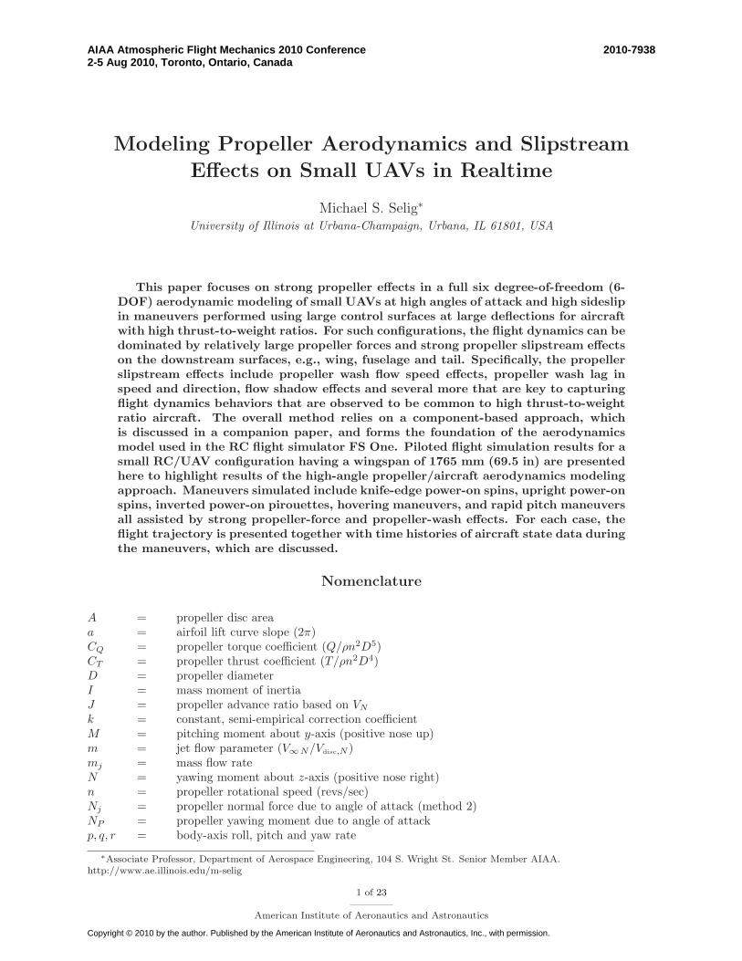
Figure 1. APC Sport 14×8 geometric characteristics and photographic projections.

II. Propeller Forces and Moments

For the normal working state (steady axial-flow conditions), the propeller thrust and torque are given by

T = ρn2D4CT (1)

Q = ρn2D5CQ (2)

where the thrust and torque coefficients are determined through lookup tables on the advance ratio given by

J =VN

nD(3)

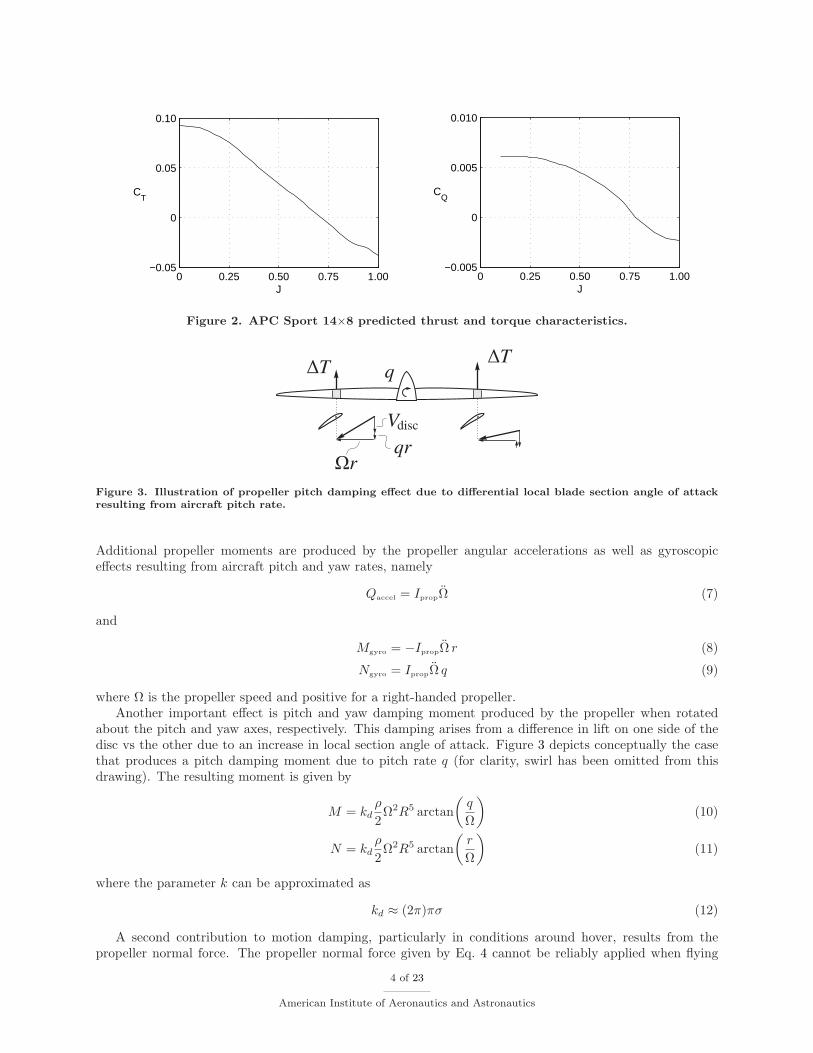
where VN is the normal component of the relative flow at the propeller disc. The propeller thrust andtorque coefficients (Eqs. 1 and 2) are determined from blade element momentum theory, in particular, usingthe code PROPID.3–5 For this analysis, the propeller chord and twist distributions are determined fromdigitized photographic projections of the top and side views as shown in Fig. 1. These data together withcorresponding propeller airfoil data are used to determine the resulting coefficient CT and CQ data. Figure 2shows these predictions for the propeller shown in Fig. 1.

Apart from the basic propeller aerodynamics expressed in Eqs. 1 and 2, a number of other factors mustbe considered for any general motion and propeller attitude. These include propeller normal force PN andP-factor (yawing moment) NP when the flow is not axial, i.e. when the propeller is at an angle of attack tothe flow. These effects are given by1

PN =σqA

2

Cl +aJ

2πln

[

1 +

(

π

J

)2]

+π

JCd

α (4)

NP =−σqAR

2

2π

3JCl +

a

2

[

1 −

(

J

π

)2

ln

(

1 +

[

π

J

]2)]

−π

JCd

α (5)

where the average lift coefficient Cl is expressed as

Cl =

(

3J

2π

)[

2

σqA

J

πT + Cd

]

(6)

3 of 23

American Institute of Aeronautics and Astronautics

0 0.25 0.50 0.75 1.00−0.05

0

0.05

0.10

J

CT

0 0.25 0.50 0.75 1.00−0.005

0

0.005

0.010

J

CQ

Figure 2. APC Sport 14×8 predicted thrust and torque characteristics.

Figure 3. Illustration of propeller pitch damping effect due to differential local blade section angle of attackresulting from aircraft pitch rate.

Additional propeller moments are produced by the propeller angular accelerations as well as gyroscopiceffects resulting from aircraft pitch and yaw rates, namely

Qaccel = IpropΩ (7)

and

Mgyro = −IpropΩ r (8)

Ngyro = IpropΩ q (9)

where Ω is the propeller speed and positive for a right-handed propeller.Another important effect is pitch and yaw damping moment produced by the propeller when rotated

about the pitch and yaw axes, respectively. This damping arises from a difference in lift on one side of thedisc vs the other due to an increase in local section angle of attack. Figure 3 depicts conceptually the casethat produces a pitch damping moment due to pitch rate q (for clarity, swirl has been omitted from thisdrawing). The resulting moment is given by

M = kd

ρ

2Ω2R5 arctan

(

q

Ω

)

(10)

N = kd

ρ

2Ω2R5 arctan

(

r

Ω

)

(11)

where the parameter k can be approximated as

kd ≈ (2π)πσ (12)

A second contribution to motion damping, particularly in conditions around hover, results from thepropeller normal force. The propeller normal force given by Eq. 4 cannot be reliably applied when flying

4 of 23

American Institute of Aeronautics and Astronautics

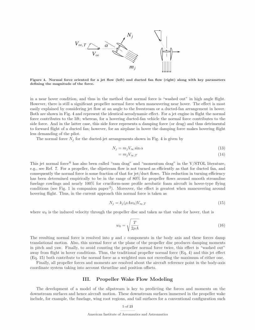
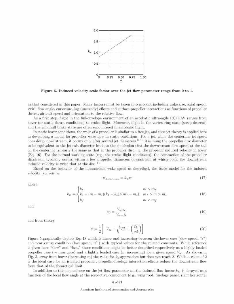
Figure 4. Normal force oriented for a jet flow (left) and ducted fan flow (right) along with key parametersdefining the magnitude of the force.

in a near hover condition, and thus in the method that normal force is “washed out” in high angle flight.However, there is still a significant propeller normal force when maneuvering near hover. The effect is mosteasily explained by considering jet flow at an angle to the freestream or a ducted-fan arrangement in hover.Both are shown in Fig. 4 and represent the identical aerodynamic effect. For a jet engine in flight the normalforce contributes to the lift; whereas, for a hovering ducted-fan vehicle the normal force contributes to theside force. And in the latter case, this side force represents a damping force (or drag) and thus detrimentalto forward flight of a ducted fan; however, for an airplane in hover the damping force makes hovering flightless demanding of the pilot.

The normal force Nj for the ducted-jet arrangements shown in Fig. 4 is given by

Nj = mjV∞ sinα (13)

= mjV∞,T (14)

This jet normal force6 has also been called “ram drag” and “momentum drag” in the V/STOL literature,e.g., see Ref. 7. For a propeller, the slipstream flow is not turned as efficiently as that for ducted fan, andconsequently the normal force is some fraction of that for jet/duct flows. This reduction in turning efficiencyhas been determined empirically to be in the range of 80% for propeller flows around smooth streamlinefuselage cowlings and nearly 100% for cruciform-nose profile aerobatic foam aircraft in hover-type flyingconditions (see Fig. 1 in companion paper2). Moreover, the effect is greatest when maneuvering aroundhovering flight. Thus, in the current approach this normal force is taken as

Nj = kj(ρAw0)V∞,T (15)

where w0 is the induced velocity through the propeller disc and taken as that value for hover, that is

w0 =

√

T

2ρA(16)

The resulting normal force is resolved into y and z components in the body axis and these forces damptranslational motion. Also, this normal force at the plane of the propeller disc produces damping momentsin pitch and yaw. Finally, to avoid counting the propeller normal force twice, this effect is “washed out”away from flight in hover conditions. Thus, the traditional propeller normal force (Eq. 4) and this jet effect(Eq. 15) both contribute to the normal force as a weighted sum not exceeding the maximum of either one.

Finally, all propeller forces and moments are resolved about the aircraft reference point in the body-axiscoordinate system taking into account thrustline and position offsets.

III. Propeller Wake Flow Modeling

The development of a model of the slipstream is key to predicting the forces and moments on thedownstream surfaces and hence aircraft motion. These downstream surfaces immersed in the propeller wakeinclude, for example, the fuselage, wing root regions, and tail surfaces for a conventional configuration such

5 of 23

American Institute of Aeronautics and Astronautics

0 0.25 0.50 0.75 1.000

0.5

1.0

1.5

2.0

m

kw

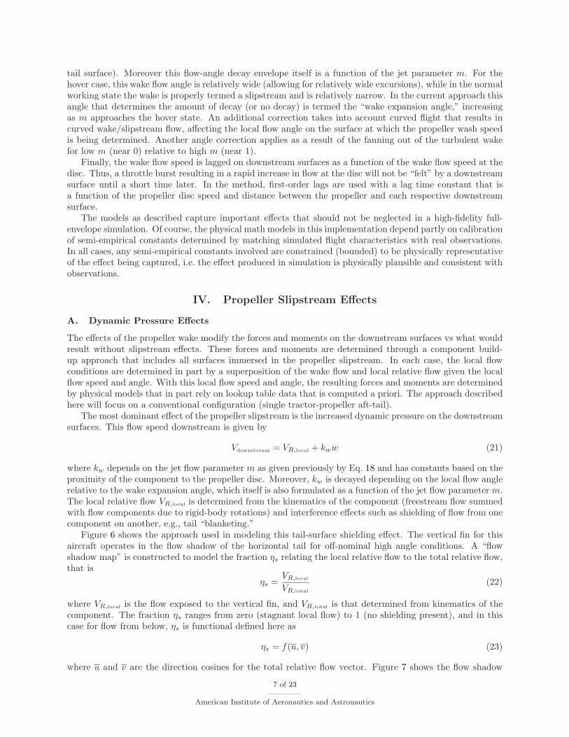
Figure 5. Induced velocity scale factor over the jet flow parameter range from 0 to 1.

as that considered in this paper. Many factors must be taken into account including wake size, axial speed,swirl, flow angle, curvature, lag (unsteady) effects and surface-propeller interactions as functions of propellerthrust, aircraft speed and orientation to the relative flow.

As a first step, flight in the full-envelope environment of an aerobatic ultra-agile RC/UAV ranges fromhover (or static thrust conditions) to cruise flight. Moreover, flight in the vortex ring state (steep descent)and the windmill brake state are often encountered in aerobatic flight.

In static hover conditions, the wake of a propeller is similar to a free jet, and thus jet theory is applied herein developing a model for propeller wake flow in static conditions. For a jet, while the centerline jet speeddoes decay downstream, it occurs only after several jet diameters.8–10 Assuming the propeller disc diameterto be equivalent to the jet exit diameter leads to the conclusion that the downstream flow speed at the tailon the centerline is nearly the same as that at the propeller disc, i.e. the propeller induced velocity in hover(Eq. 16). For the normal working state (e.g., the cruise flight conditions), the contraction of the propellerslipstream typically occurs within a few propeller diameters downstream at which point the downstreaminduced velocity is twice that at the disc.11

Based on the behavior of the downstream wake speed as described, the basic model for the inducedvelocity is given by

wdownstream = kww (17)

where

kw =

ks m < ms

ks + (m−ms)(kf − ks)/(mf −ms) mf > m > ms

kf m > mf

(18)

and

m =V∞N

Vdisc,N

(19)

and from theory

w =1

2

[

−V∞ +

√

V 2∞ +

(

2T

ρA

)]

(20)

Figure 5 graphically depicts Eq. 18 which is linear and increasing between the hover case (slow speed, “s”)and near cruise condition (fast speed, “f”) with typical values for the related constants. While referenceis given here “slow” and “fast,” these conditions might be better described respectively as a highly loadedpropeller case (m near zero) and a lightly loaded case (m increasing) for a given speed V∞. As shown inFig. 5, away from hover (increasing m) the value for ks approaches but does not reach 2. While a value of 2is the ideal case for an isolated propeller, propeller-fuselage interaction effects reduce the downstream flowfrom that of the theoretical limit.

In addition to this dependence on the jet flow parameter m, the induced flow factor kw is decayed as afunction of the local flow angle at the respective component (e.g., wing root, fuselage panel, right horizontal

6 of 23

American Institute of Aeronautics and Astronautics

tail surface). Moreover this flow-angle decay envelope itself is a function of the jet parameter m. For thehover case, this wake flow angle is relatively wide (allowing for relatively wide excursions), while in the normalworking state the wake is properly termed a slipstream and is relatively narrow. In the current approach thisangle that determines the amount of decay (or no decay) is termed the “wake expansion angle,” increasingas m approaches the hover state. An additional correction takes into account curved flight that results incurved wake/slipstream flow, affecting the local flow angle on the surface at which the propeller wash speedis being determined. Another angle correction applies as a result of the fanning out of the turbulent wakefor low m (near 0) relative to high m (near 1).

Finally, the wake flow speed is lagged on downstream surfaces as a function of the wake flow speed at thedisc. Thus, a throttle burst resulting in a rapid increase in flow at the disc will not be “felt” by a downstreamsurface until a short time later. In the method, first-order lags are used with a lag time constant that isa function of the propeller disc speed and distance between the propeller and each respective downstreamsurface.

The models as described capture important effects that should not be neglected in a high-fidelity full-envelope simulation. Of course, the physical math models in this implementation depend partly on calibrationof semi-empirical constants determined by matching simulated flight characteristics with real observations.In all cases, any semi-empirical constants involved are constrained (bounded) to be physically representativeof the effect being captured, i.e. the effect produced in simulation is physically plausible and consistent withobservations.

IV. Propeller Slipstream Effects

A. Dynamic Pressure Effects

The effects of the propeller wake modify the forces and moments on the downstream surfaces vs what wouldresult without slipstream effects. These forces and moments are determined through a component build-up approach that includes all surfaces immersed in the propeller slipstream. In each case, the local flowconditions are determined in part by a superposition of the wake flow and local relative flow given the localflow speed and angle. With this local flow speed and angle, the resulting forces and moments are determinedby physical models that in part rely on lookup table data that is computed a priori. The approach describedhere will focus on a conventional configuration (single tractor-propeller aft-tail).

The most dominant effect of the propeller slipstream is the increased dynamic pressure on the downstreamsurfaces. This flow speed downstream is given by

Vdownstream = VR,local + kww (21)

where kw depends on the jet flow parameter m as given previously by Eq. 18 and has constants based on theproximity of the component to the propeller disc. Moreover, kw is decayed depending on the local flow anglerelative to the wake expansion angle, which itself is also formulated as a function of the jet flow parameter m.The local relative flow VR,local is determined from the kinematics of the component (freestream flow summedwith flow components due to rigid-body rotations) and interference effects such as shielding of flow from onecomponent on another, e.g., tail “blanketing.”

Figure 6 shows the approach used in modeling this tail-surface shielding effect. The vertical fin for thisaircraft operates in the flow shadow of the horizontal tail for off-nominal high angle conditions. A “flowshadow map” is constructed to model the fraction ηs relating the local relative flow to the total relative flow,that is

ηs =VR,local

VR,total

(22)

where VR,local is the flow exposed to the vertical fin, and VR,total is that determined from kinematics of thecomponent. The fraction ηs ranges from zero (stagnant local flow) to 1 (no shielding present), and in thiscase for flow from below, ηs is functional defined here as

ηs = f(u, v) (23)

where u and v are the direction cosines for the total relative flow vector. Figure 7 shows the flow shadow

7 of 23

American Institute of Aeronautics and Astronautics

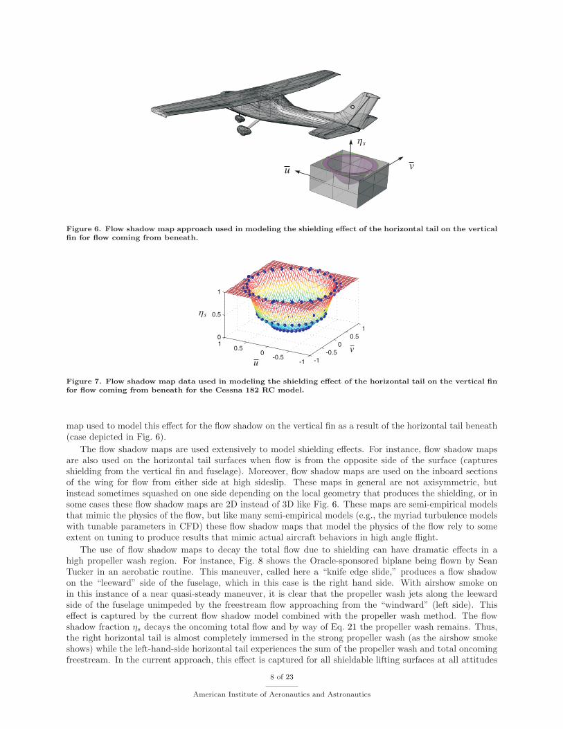
Figure 6. Flow shadow map approach used in modeling the shielding effect of the horizontal tail on the verticalfin for flow coming from beneath.

Figure 7. Flow shadow map data used in modeling the shielding effect of the horizontal tail on the vertical finfor flow coming from beneath for the Cessna 182 RC model.

map used to model this effect for the flow shadow on the vertical fin as a result of the horizontal tail beneath(case depicted in Fig. 6).

The flow shadow maps are used extensively to model shielding effects. For instance, flow shadow mapsare also used on the horizontal tail surfaces when flow is from the opposite side of the surface (capturesshielding from the vertical fin and fuselage). Moreover, flow shadow maps are used on the inboard sectionsof the wing for flow from either side at high sideslip. These maps in general are not axisymmetric, butinstead sometimes squashed on one side depending on the local geometry that produces the shielding, or insome cases these flow shadow maps are 2D instead of 3D like Fig. 6. These maps are semi-empirical modelsthat mimic the physics of the flow, but like many semi-empirical models (e.g., the myriad turbulence modelswith tunable parameters in CFD) these flow shadow maps that model the physics of the flow rely to someextent on tuning to produce results that mimic actual aircraft behaviors in high angle flight.

The use of flow shadow maps to decay the total flow due to shielding can have dramatic effects in ahigh propeller wash region. For instance, Fig. 8 shows the Oracle-sponsored biplane being flown by SeanTucker in an aerobatic routine. This maneuver, called here a “knife edge slide,” produces a flow shadowon the “leeward” side of the fuselage, which in this case is the right hand side. With airshow smoke onin this instance of a near quasi-steady maneuver, it is clear that the propeller wash jets along the leewardside of the fuselage unimpeded by the freestream flow approaching from the “windward” (left side). Thiseffect is captured by the current flow shadow model combined with the propeller wash method. The flowshadow fraction ηs decays the oncoming total flow and by way of Eq. 21 the propeller wash remains. Thus,the right horizontal tail is almost completely immersed in the strong propeller wash (as the airshow smokeshows) while the left-hand-side horizontal tail experiences the sum of the propeller wash and total oncomingfreestream. In the current approach, this effect is captured for all shieldable lifting surfaces at all attitudes

8 of 23

American Institute of Aeronautics and Astronautics

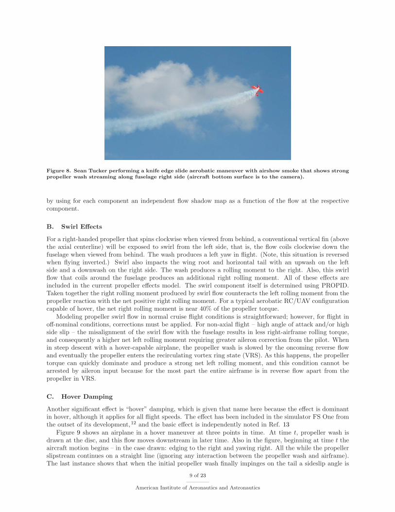
Figure 8. Sean Tucker performing a knife edge slide aerobatic maneuver with airshow smoke that shows strongpropeller wash streaming along fuselage right side (aircraft bottom surface is to the camera).

by using for each component an independent flow shadow map as a function of the flow at the respectivecomponent.

B. Swirl Effects

For a right-handed propeller that spins clockwise when viewed from behind, a conventional vertical fin (abovethe axial centerline) will be exposed to swirl from the left side, that is, the flow coils clockwise down thefuselage when viewed from behind. The wash produces a left yaw in flight. (Note, this situation is reversedwhen flying inverted.) Swirl also impacts the wing root and horizontal tail with an upwash on the leftside and a downwash on the right side. The wash produces a rolling moment to the right. Also, this swirlflow that coils around the fuselage produces an additional right rolling moment. All of these effects areincluded in the current propeller effects model. The swirl component itself is determined using PROPID.Taken together the right rolling moment produced by swirl flow counteracts the left rolling moment from thepropeller reaction with the net positive right rolling moment. For a typical aerobatic RC/UAV configurationcapable of hover, the net right rolling moment is near 40% of the propeller torque.

Modeling propeller swirl flow in normal cruise flight conditions is straightforward; however, for flight inoff-nominal conditions, corrections must be applied. For non-axial flight – high angle of attack and/or highside slip – the misalignment of the swirl flow with the fuselage results in less right-airframe rolling torque,and consequently a higher net left rolling moment requiring greater aileron correction from the pilot. Whenin steep descent with a hover-capable airplane, the propeller wash is slowed by the oncoming reverse flowand eventually the propeller enters the recirculating vortex ring state (VRS). As this happens, the propellertorque can quickly dominate and produce a strong net left rolling moment, and this condition cannot bearrested by aileron input because for the most part the entire airframe is in reverse flow apart from thepropeller in VRS.

C. Hover Damping

Another significant effect is “hover” damping, which is given that name here because the effect is dominantin hover, although it applies for all flight speeds. The effect has been included in the simulator FS One fromthe outset of its development,12 and the basic effect is independently noted in Ref. 13

Figure 9 shows an airplane in a hover maneuver at three points in time. At time t, propeller wash isdrawn at the disc, and this flow moves downstream in later time. Also in the figure, beginning at time t theaircraft motion begins – in the case drawn: edging to the right and yawing right. All the while the propellerslipstream continues on a straight line (ignoring any interaction between the propeller wash and airframe).The last instance shows that when the initial propeller wash finally impinges on the tail a sideslip angle is

9 of 23

American Institute of Aeronautics and Astronautics

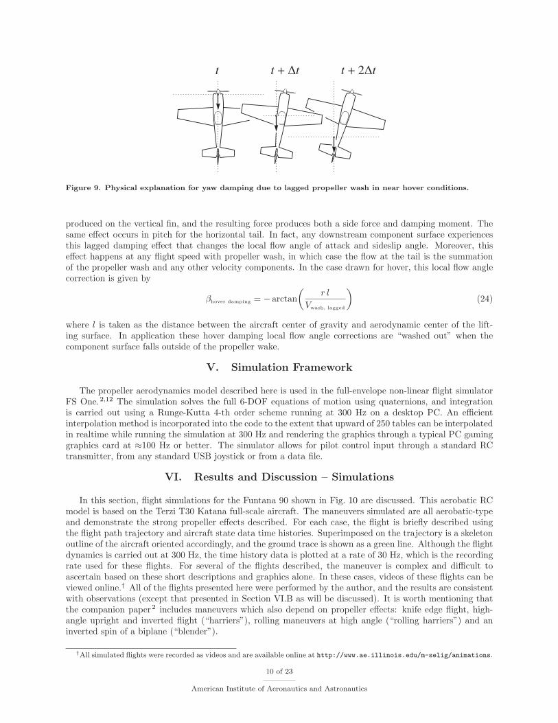
Figure 9. Physical explanation for yaw damping due to lagged propeller wash in near hover conditions.

produced on the vertical fin, and the resulting force produces both a side force and damping moment. Thesame effect occurs in pitch for the horizontal tail. In fact, any downstream component surface experiencesthis lagged damping effect that changes the local flow angle of attack and sideslip angle. Moreover, thiseffect happens at any flight speed with propeller wash, in which case the flow at the tail is the summationof the propeller wash and any other velocity components. In the case drawn for hover, this local flow anglecorrection is given by

βhover damping = − arctan

(

r l

Vwash, lagged

)

(24)

where l is taken as the distance between the aircraft center of gravity and aerodynamic center of the lift-ing surface. In application these hover damping local flow angle corrections are “washed out” when thecomponent surface falls outside of the propeller wake.

V. Simulation Framework

The propeller aerodynamics model described here is used in the full-envelope non-linear flight simulatorFS One.2,12 The simulation solves the full 6-DOF equations of motion using quaternions, and integrationis carried out using a Runge-Kutta 4-th order scheme running at 300 Hz on a desktop PC. An efficientinterpolation method is incorporated into the code to the extent that upward of 250 tables can be interpolatedin realtime while running the simulation at 300 Hz and rendering the graphics through a typical PC gaminggraphics card at ≈100 Hz or better. The simulator allows for pilot control input through a standard RCtransmitter, from any standard USB joystick or from a data file.

VI. Results and Discussion – Simulations

In this section, flight simulations for the Funtana 90 shown in Fig. 10 are discussed. This aerobatic RCmodel is based on the Terzi T30 Katana full-scale aircraft. The maneuvers simulated are all aerobatic-typeand demonstrate the strong propeller effects described. For each case, the flight is briefly described usingthe flight path trajectory and aircraft state data time histories. Superimposed on the trajectory is a skeletonoutline of the aircraft oriented accordingly, and the ground trace is shown as a green line. Although the flightdynamics is carried out at 300 Hz, the time history data is plotted at a rate of 30 Hz, which is the recordingrate used for these flights. For several of the flights described, the maneuver is complex and difficult toascertain based on these short descriptions and graphics alone. In these cases, videos of these flights can beviewed online.† All of the flights presented here were performed by the author, and the results are consistentwith observations (except that presented in Section VI.B as will be discussed). It is worth mentioning thatthe companion paper2 includes maneuvers which also depend on propeller effects: knife edge flight, high-angle upright and inverted flight (“harriers”), rolling maneuvers at high angle (“rolling harriers”) and aninverted spin of a biplane (“blender”).

†All simulated flights were recorded as videos and are available online at http://www.ae.illinois.edu/m-selig/animations.

10 of 23

American Institute of Aeronautics and Astronautics

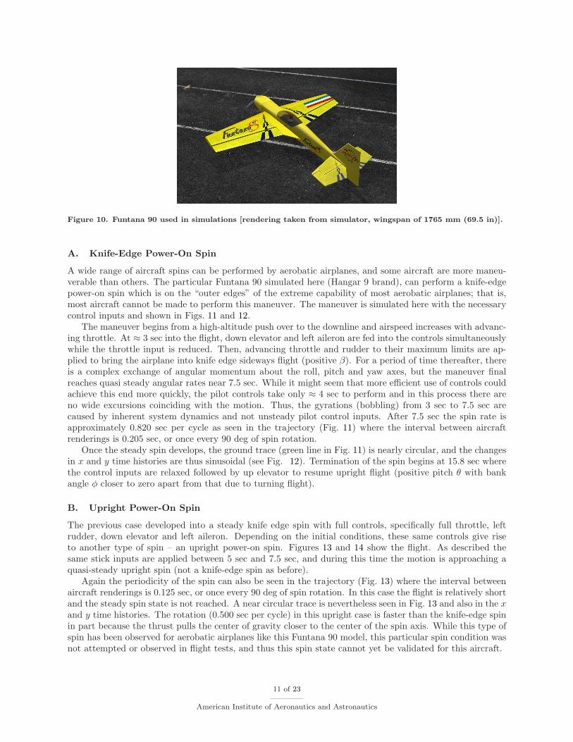
Figure 10. Funtana 90 used in simulations [rendering taken from simulator, wingspan of 1765 mm (69.5 in)].

A. Knife-Edge Power-On Spin

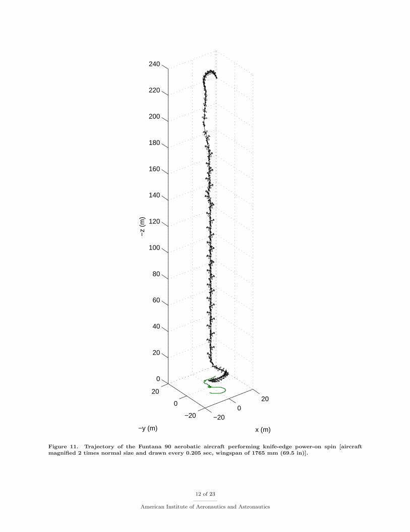
A wide range of aircraft spins can be performed by aerobatic airplanes, and some aircraft are more maneu-verable than others. The particular Funtana 90 simulated here (Hangar 9 brand), can perform a knife-edgepower-on spin which is on the “outer edges” of the extreme capability of most aerobatic airplanes; that is,most aircraft cannot be made to perform this maneuver. The maneuver is simulated here with the necessarycontrol inputs and shown in Figs. 11 and 12.

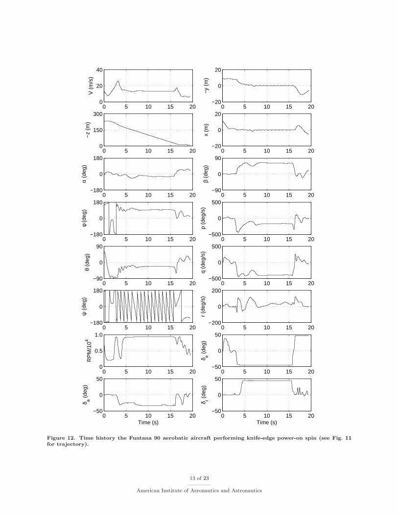
The maneuver begins from a high-altitude push over to the downline and airspeed increases with advanc-ing throttle. At ≈ 3 sec into the flight, down elevator and left aileron are fed into the controls simultaneouslywhile the throttle input is reduced. Then, advancing throttle and rudder to their maximum limits are ap-plied to bring the airplane into knife edge sideways flight (positive β). For a period of time thereafter, thereis a complex exchange of angular momentum about the roll, pitch and yaw axes, but the maneuver finalreaches quasi steady angular rates near 7.5 sec. While it might seem that more efficient use of controls couldachieve this end more quickly, the pilot controls take only ≈ 4 sec to perform and in this process there areno wide excursions coinciding with the motion. Thus, the gyrations (bobbling) from 3 sec to 7.5 sec arecaused by inherent system dynamics and not unsteady pilot control inputs. After 7.5 sec the spin rate isapproximately 0.820 sec per cycle as seen in the trajectory (Fig. 11) where the interval between aircraftrenderings is 0.205 sec, or once every 90 deg of spin rotation.

Once the steady spin develops, the ground trace (green line in Fig. 11) is nearly circular, and the changesin x and y time histories are thus sinusoidal (see Fig. 12). Termination of the spin begins at 15.8 sec wherethe control inputs are relaxed followed by up elevator to resume upright flight (positive pitch θ with bankangle φ closer to zero apart from that due to turning flight).

B. Upright Power-On Spin

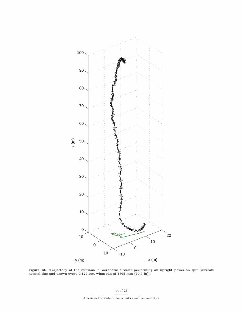
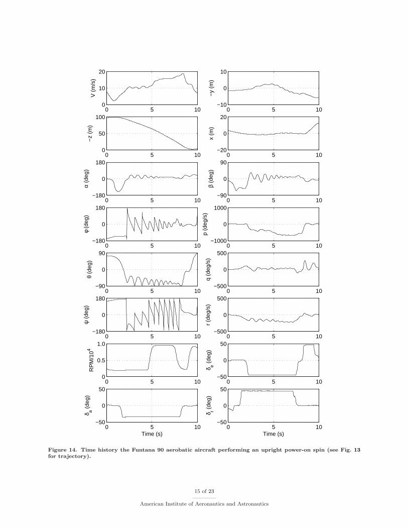
The previous case developed into a steady knife edge spin with full controls, specifically full throttle, leftrudder, down elevator and left aileron. Depending on the initial conditions, these same controls give riseto another type of spin – an upright power-on spin. Figures 13 and 14 show the flight. As described thesame stick inputs are applied between 5 sec and 7.5 sec, and during this time the motion is approaching aquasi-steady upright spin (not a knife-edge spin as before).

Again the periodicity of the spin can also be seen in the trajectory (Fig. 13) where the interval betweenaircraft renderings is 0.125 sec, or once every 90 deg of spin rotation. In this case the flight is relatively shortand the steady spin state is not reached. A near circular trace is nevertheless seen in Fig. 13 and also in the xand y time histories. The rotation (0.500 sec per cycle) in this upright case is faster than the knife-edge spinin part because the thrust pulls the center of gravity closer to the center of the spin axis. While this type ofspin has been observed for aerobatic airplanes like this Funtana 90 model, this particular spin condition wasnot attempted or observed in flight tests, and thus this spin state cannot yet be validated for this aircraft.

11 of 23

American Institute of Aeronautics and Astronautics

−200

20

−20

0

20

0

20

40

60

80

100

120

140

160

180

200

220

240

x (m)−y (m)

−z

(m)

Figure 11. Trajectory of the Funtana 90 aerobatic aircraft performing knife-edge power-on spin [aircraftmagnified 2 times normal size and drawn every 0.205 sec, wingspan of 1765 mm (69.5 in)].

12 of 23

American Institute of Aeronautics and Astronautics

0 5 10 15 20−50

0

50

Time (s)

δ a (de

g)

0 5 10 15 20−50

0

50

Time (s)

δ r (de

g)

0 5 10 15 200

0.5

1.0

RP

M/1

04

0 5 10 15 20−50

0

50

δ e (de

g)

0 5 10 15 20−180

0

180

ψ (

deg)

0 5 10 15 20−200

0

200

r (d

eg/s

)

0 5 10 15 20−90

0

90

θ (d

eg)

0 5 10 15 20−500

0

500

q (d

eg/s

)

0 5 10 15 20−180

0

180

φ (d

eg)

0 5 10 15 20−500

0

500p

(deg

/s)

0 5 10 15 20−180

0

180

α (d

eg)

0 5 10 15 20−90

0

90

β (d

eg)

0 5 10 15 200

150

300

−z

(m)

0 5 10 15 20−20

0

20

x (m

)

0 5 10 15 200

20

40

V (

m/s

)

0 5 10 15 20−20

0

20

−y

(m)

Figure 12. Time history the Funtana 90 aerobatic aircraft performing knife-edge power-on spin (see Fig. 11for trajectory).

13 of 23

American Institute of Aeronautics and Astronautics

−10

0

10

20

−10

0

10

0

10

20

30

40

50

60

70

80

90

100

x (m)−y (m)

−z

(m)

Figure 13. Trajectory of the Funtana 90 aerobatic aircraft performing an upright power-on spin [aircraftnormal size and drawn every 0.125 sec, wingspan of 1765 mm (69.5 in)].

14 of 23

American Institute of Aeronautics and Astronautics

0 5 10−50

0

50

Time (s)

δ a (de

g)

0 5 10−50

0

50

Time (s)

δ r (de

g)

0 5 100

0.5

1.0

RP

M/1

04

0 5 10−50

0

50

δ e (de

g)

0 5 10−180

0

180

ψ (

deg)

0 5 10−500

0

500

r (d

eg/s

)

0 5 10−90

0

90

θ (d

eg)

0 5 10−500

0

500

q (d

eg/s

)

0 5 10−180

0

180

φ (d

eg)

0 5 10−1000

0

1000p

(deg

/s)

0 5 10−180

0

180

α (d

eg)

0 5 10−90

0

90

β (d

eg)

0 5 100

50

100

−z

(m)

0 5 10−20

0

20

x (m

)

0 5 100

10

20

V (

m/s

)

0 5 10−10

0

10

−y

(m)

Figure 14. Time history the Funtana 90 aerobatic aircraft performing an upright power-on spin (see Fig. 13for trajectory).

15 of 23

American Institute of Aeronautics and Astronautics

−10

−5

0

5

−30−25

−20−15

−10−5

05

10

0

5

10

15

20

25

−y (m)x (m)

−z

(m)

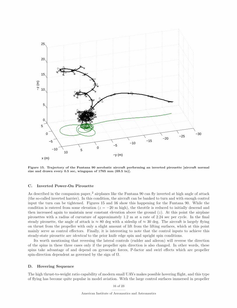
Figure 15. Trajectory of the Funtana 90 aerobatic aircraft performing an inverted pirouette [aircraft normalsize and drawn every 0.5 sec, wingspan of 1765 mm (69.5 in)].

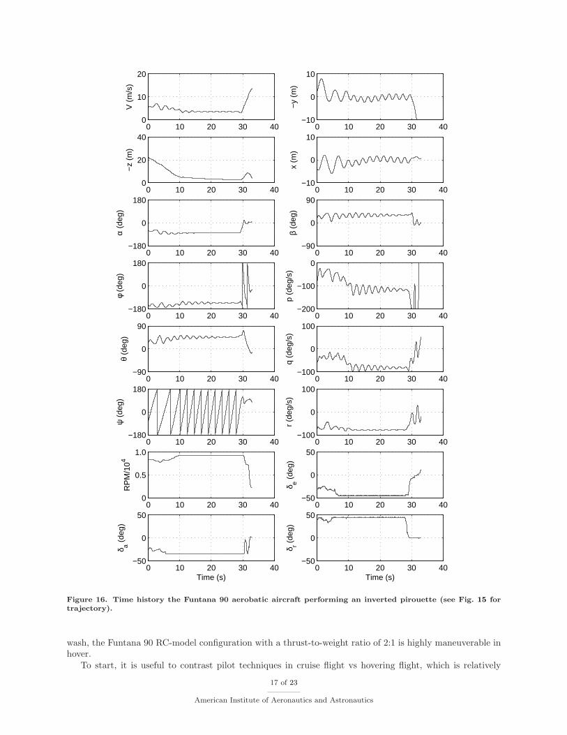
C. Inverted Power-On Pirouette

As described in the companion paper,2 airplanes like the Funtana 90 can fly inverted at high angle of attack(the so-called inverted harrier). In this condition, the aircraft can be banked to turn and with enough controlinput the turn can be tightened. Figures 15 and 16 show this happening for the Funtana 90. While thecondition is entered from some elevation (z = −20 m high), the throttle is reduced to initially descend andthen increased again to maintain near constant elevation above the ground (z). At this point the airplanepirouettes with a radius of curvature of approximately 1.2 m at a rate of 2.24 sec per cycle. In the finalsteady pirouette, the angle of attack is ≈ 80 deg with a sideslip of ≈ 30 deg. The aircraft is largely flyingon thrust from the propeller with only a slight amount of lift from the lifting surfaces, which at this pointmainly serve as control effectors. Finally, it is interesting to note that the control inputs to achieve thissteady-state pirouette are identical to the prior knife edge spin and upright spin conditions.

Its worth mentioning that reversing the lateral controls (rudder and aileron) will reverse the directionof the spins in these three cases only if the propeller spin direction is also changed. In other words, thesespins take advantage of and depend on gyroscopic forces, P-factor and swirl effects which are propellerspin-direction dependent as governed by the sign of Ω.

D. Hovering Sequence

The high thrust-to-weight ratio capability of modern small UAVs makes possible hovering flight, and this typeof flying has become quite popular in model aviation. With the large control surfaces immersed in propeller

16 of 23

American Institute of Aeronautics and Astronautics

0 10 20 30 40−50

0

50

Time (s)

δ a (de

g)

0 10 20 30 40−50

0

50

Time (s)

δ r (de

g)

0 10 20 30 400

0.5

1.0

RP

M/1

04

0 10 20 30 40−50

0

50

δ e (de

g)

0 10 20 30 40−180

0

180

ψ (

deg)

0 10 20 30 40−100

0

100

r (d

eg/s

)

0 10 20 30 40−90

0

90

θ (d

eg)

0 10 20 30 40−100

0

100

q (d

eg/s

)

0 10 20 30 40−180

0

180

φ (d

eg)

0 10 20 30 40−200

−100

0

p (d

eg/s

)

0 10 20 30 40−180

0

180

α (d

eg)

0 10 20 30 40−90

0

90

β (d

eg)

0 10 20 30 400

20

40−

z (m

)

0 10 20 30 40−10

0

10

x (m

)

0 10 20 30 400

10

20

V (

m/s

)0 10 20 30 40

−10

0

10

−y

(m)

Figure 16. Time history the Funtana 90 aerobatic aircraft performing an inverted pirouette (see Fig. 15 fortrajectory).

wash, the Funtana 90 RC-model configuration with a thrust-to-weight ratio of 2:1 is highly maneuverable inhover.

To start, it is useful to contrast pilot techniques in cruise flight vs hovering flight, which is relatively

17 of 23

American Institute of Aeronautics and Astronautics

new and being advanced by high-performance RC models. In normal cruise flight, as noted in Ref. 6, theelevator and rudder are displacement controls used to set a trim position. The ailerons, however, are a ratecontrol used to set the roll rate. In hovering flight, however, the elevator, rudder and ailerons all becomerate controls. Moreover, in hover, the aircraft is never in vertical trim; it is always unstable, tending to moveoff of perfect vertical alignment. Thus, the two modes of flight (cruise vs hover) are quite different, and itrequires a change in piloting strategy (mental thinking and control inputs) when switching between the two.Another, observation involving pilot strategy is that pilots in hover regularly pulse the throttle command.This technique allows a pilot to continuously gauge the control power (maneuver power) of the airplane andthus anticipate and maneuver through any dynamic response. Of course, while these modes of flight aredistinctly different, flying back and forth between these two regimes becomes second nature for experiencedpilots.

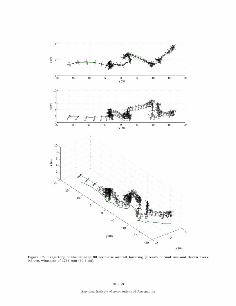
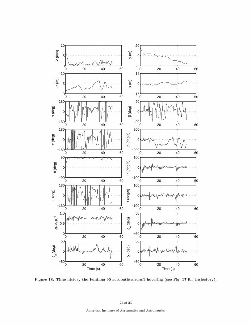
As shown in Fig. 17, the trajectory plot is cluttered because of the near stationary flight for certainperiods in the sequence. There are three main hovering stages that make up this full hovering sequence. Forthe entire time history shown in Fig. 18, the airplane pitch is ≈ 90 deg – pointed straight up. Also, for theentire sequence, small inputs on elevator and rudder are used to maintain the 90-deg hovering attitude andmaintain a sense of pitch and yaw control power at any given point in time.

In the first stage from 2.7 to 13.4 sec, the control strategy was to maintain the aircraft orientationas ‘top-side’ to the pilot, i.e. near zero roll rate (p) while keeping the aircraft in top-view position fromthe perspective of the pilot. In this position, without any aileron input, the aircraft will roll left due topropeller torque and the counteracting, but smaller, aerodynamic torques from downstream surfaces. Thus,to maintain the orientation, right aileron pulses are used continuously to zero the net rolling moment. Asdescribed, these inputs are also pulsed (see spikes in δa) to maintain a constant sense of control power.During this period of time, the x-y position changes little because the aircraft is in hover.

The second stage of hover begins when the airplane reaches the position −y = −2.5 m (see side view inFig. 17). During this time, which begins around 20 sec, no aileron input (δa) is applied, and the airplaneenters a slow torque roll at a rate of p ≈ −100 deg/sec. Only rudder and elevator deflections are applied tomaintain the 90-deg vertical pitch.

Finally, for the third stage, the airplane moves to the position −y = −10 m (see side view in Fig. 17)and is allowed to climb to a height of 6.7 m. At this point, the airplane is allow to descend vertically andenter the propeller vortex ring state. When this happens, hovering in this regime is difficult for the pilot,and the control inputs are excited by the pilot while managing the rapid increase in roll rate. This descentthrough the vortex ring state happens three times ending at 50 sec, and each time the roll rate increasesafter starting from near zero.

E. Power-Effects Sequence

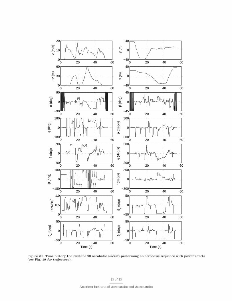
In this last sequence (Figs. 19 and 20), a number power-effects maneuvers are presented. These effects andothers will be described. For the first few seconds,‡ the airplane moves as the propeller is ‘started’ andthe control surfaces are ‘wiggles,’ which are ritual acts for a pilot. As the airplane rests on the ground theangle of attack and side slip are ill-defined as seen by the ‘chatter’ in the initial and final data in their timehistories.

After takeoff the airplane is rolled inverted with cross-controls on aileron and rudder (t = 6.4 sec). At10 sec, a burst of throttle and down elevator are used to rapidly pitch the aircraft vertical (see Fig. 19),followed by a 180-deg roll at 12.6 sec. As the airplane climbs, the throttle is reduced and the airspeed slowsto near zero. At this point in the climb where z peaks (17.2 sec), a burst of throttle and down elevator areused to pitch the airplane straight down rather than entering a tail slide condition. At the bottom of thedownline at 19.5 sec, elevator and throttle are again used to rapidly pitch the airplane. These rapid pitchmaneuvers (also seen in q and θ) are a result of strong propeller wash effects impinging on the horizontaltail with appropriate surface deflections.

‡In the simulation at t = 0 sec the airplane is placed on the ground which includes random elevation perturbations tosimulate bumpy ground. The airplane thus rocks in roll (p) when the sequence begins. At 1 sec, throttle is pulsed to ‘start’ theengine and the propeller accelerates, which produces another small wing rock (p). At 3.2 sec, the control surfaces (sticks) arewiggled, and again the wing rocks – this time due to the inertia of the aileron motions and tail wag from tail wheel motion tiedto the rudder.

18 of 23

American Institute of Aeronautics and Astronautics

The next significant propeller-effects maneuver begins after climbing to the position near x = −30 m(30 sec). At this point, full throttle, full right rudder, full down elevator and some left aileron are used toenter a near-zero-pitch inverted turning descent. At this point if throttle were reduced the aircraft wouldenter a flat spin, but with continued full throttle to show propeller effects the airplane pitches over (near42 sec) and is flown to a landing (see Fig. 19) at the pilot position.

VII. Conclusions

As described in this paper, traditional propeller effects and new effects from strong propeller wash areimportant in simulating flight dynamics over the full ±180 deg high-angle full-envelope flight considered here.These propeller effects include not only the traditionally considered thrust, torque and normal force but alsoimportant slipstream and momentum effects that dominate in low-speed to hovering conditions. In particular,there are several damping forces and moments that affect the handling qualities in and around slow-speedand hovering flight. Piloted flight simulation results for a small RC/UAV configuration demonstrate thatthese important effects drive the flight dynamics in a number of maneuvers, which was shown here withknife-edge power-on spins, upright power-on spins, inverted power-on pirouettes, hovering maneuvers, andrapid pitch maneuvers that were all assisted by strong propeller-force and propeller-wash effects. The overallapproach that factors in many considerations is made viable by incorporating this propeller model in a largeraerodynamics component-based simulation framework that is discussed in a companion paper.

Acknowledgments

The author would like to thank Brian W. Fuesz and Chris A. Lyon for programming the framework ofthe simulator that includes the methods described in this paper. Also, the aircraft design and developmentgroup at Horizon Hobby is gratefully acknowledged for partly supporting the initial development of thesimulator. The author wishes to acknowledge Pritam P. Sukumar for his efforts in assisting in preparationof some of the plots included in this paper.

References

1McCormick, B. W., Aerodynamics, Aeronautics, and Flight Mechanics, John Wiley & Sons, New York, 2nd ed., 1995.2Selig, M. S., “Modeling Full-Envelope Aerodynamics of Small UAVs in Realtime,” AIAA Paper 2010–7635, August 2010.3Hibbs, B. and Radkey, R. L., “Calculating Rotor Performance with the Revised PROP Computer Code,” Tech. rep.,

Wind Energy Research Center, Rockwell International, Golden, CO, RFP-3508, UC-60, 1983.4Selig, M. S. and Tangler, J. L., “Development and Application of a Multipoint Inverse Design Method for Horizontal

Axis Wind Turbines,” Wind Engineering, Vol. 19, No. 5, 1995, pp. 91–105.5Selig, M. S., “PROPID - Software for Horizontal-Axis Wind Turbine Design and Analysis,”

http://www.ae.illinois.edu/m-selig/propid.html, 1995–.6Etkin, B. and Reid, L. D., Dynamics of Flight – Stability and Control , John Wiley & Sons, New York, 2nd ed., 1995.7Guerrero, I., Londenberg, K., Gelhausen, P., and Myklebust, A., “A Powered Lift Aerodynamic Analysis for the Design

of Ducted Fan UAVs,” AIAA Paper 2003–6567, September 2003.8Abramovich, G. N., The Theory of Turbulent Jets, The MIT Press, Cambridge, MA, 1963.9Schetz, J. A., Injection and Mixing in Turbulent Flow), series = AIAA Progress in Astronautics and Aeronautics,

publisher = AIAA, Reston, VA, year = 1980,.10Kuhn, R. E., Margason, R. J., and Curtis, P., Jet Induced Effects: The Aerodynamics of Jet and Fan Powered V/STOL

Aircraft in Hover and Transition, AIAA Progress in Astronautics and Aeronautics, AIAA, Reston, VA, 2006.11Veldhuis, L. L. M., Propeller Wind Aerodynamic Interference, Ph.D. thesis, Department of Aerospace Engineering, Delft

University of Technology, The Netherlands, 2005.12“FS One, Precision RC Flight Simulator,” Software Developed by InertiaSoft, Distributed by Horizon Hobby, Champaign,

IL, 2006.13Frank, A., McGrew, J. S., Valenti, M., Levine, D., and How, J. P., “Hover, Transition, and Level Flight Control Design

for a Single-Propeller Indoor Airplane,” AIAA Paper 2007–6318, August 2007.

19 of 23

American Institute of Aeronautics and Astronautics

−5

0

5

−20−15−10−505101520−y (m)

x (m

)

−20−15−10−5051015200

2

4

6

8

10

−y (m)

−z

(m)

−5

0

5

−20

−15

−10

−5

0

5

10

15

20

0

2

4

6

8

10

x (m)

−y (m)

−z

(m)

Figure 17. Trajectory of the Funtana 90 aerobatic aircraft hovering [aircraft normal size and drawn every0.5 sec, wingspan of 1765 mm (69.5 in)].

20 of 23

American Institute of Aeronautics and Astronautics

0 20 40 60−50

0

50

Time (s)

δ a (de

g)

0 20 40 60−50

0

50

Time (s)

δ r (de

g)

0 20 40 600

0.5

1.0

RP

M/1

04

0 20 40 60−50

0

50

δ e (de

g)

0 20 40 60−180

0

180

ψ (

deg)

0 20 40 60−100

0

100

r (d

eg/s

)

0 20 40 60−90

0

90

θ (d

eg)

0 20 40 60−100

0

100

q (d

eg/s

)

0 20 40 60−180

0

180

φ (d

eg)

0 20 40 60−200

0

200p

(deg

/s)

0 20 40 60−180

0

180

α (d

eg)

0 20 40 60−90

0

90

β (d

eg)

0 20 40 600

5

10

−z

(m)

0 20 40 60−15

0

15

x (m

)

0 20 40 600

5

10

V (

m/s

)

0 20 40 60−20

0

20

−y

(m)

Figure 18. Time history the Funtana 90 aerobatic aircraft hovering (see Fig. 17 for trajectory).

21 of 23

American Institute of Aeronautics and Astronautics

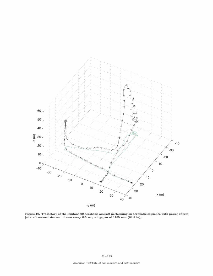
Figure 19. Trajectory of the Funtana 90 aerobatic aircraft performing an aerobatic sequence with power effects[aircraft normal size and drawn every 0.5 sec, wingspan of 1765 mm (69.5 in)].

22 of 23

American Institute of Aeronautics and Astronautics

0 20 40 60−50

0

50

Time (s)

δ a (de

g)

0 20 40 60−50

0

50

Time (s)

δ r (de

g)

0 20 40 600

0.5

1.0

RP

M/1

04

0 20 40 60−50

0

50

δ e (de

g)

0 20 40 60−180

0

180

ψ (

deg)

0 20 40 60−300

0

300

r (d

eg/s

)

0 20 40 60−90

0

90

θ (d

eg)

0 20 40 60−300

0

300

q (d

eg/s

)

0 20 40 60−180

0

180

φ (d

eg)

0 20 40 60−300

0

300p

(deg

/s)

0 20 40 60−90

0

90

α (d

eg)

0 20 40 60−45

0

45

β (d

eg)

0 20 40 600

30

60

−z

(m)

0 20 40 60−40

0

40

x (m

)

0 20 40 600

10

20

V (

m/s

)

0 20 40 60−40

0

40

−y

(m)

Figure 20. Time history the Funtana 90 aerobatic aircraft performing an aerobatic sequence with power effects(see Fig. 19 for trajectory).

23 of 23

American Institute of Aeronautics and Astronautics