Modeling of an Automotive Air Conditioning Compressor ... · Modeling of an Automotive Air Conditioning Compressor Based on Experimental Data Joseph Hale Darr Department of Mechanical

Modeling of an Automotive Air Conditioning Compressor Based on Experimental Data

ACRCTR-14

For additional information:

Air Conditioning and Refrigeration Center University of Illinois Mechanical & Industrial Engineering Dept. 1206 West Green Street Urbana,IL 61801

(217) 333-3115

J. H. Darr and R. R. Crawford

February 1992

Prepared as part of ACRC Project 09 Mobile Air Conditioning Systems

R. R. Crawford, Principal Investigator

The Air Conditioning and Refrigeration Center was founded in 1988 with a grant from the estate of Richard W. Kritzer, the founder of Peerless of America Inc. A State of Illinois Technology Challenge Grant helped build the laboratory facilities. The ACRC receives continuing support from the Richard W. Kritzer Endowment and the National Science Foundation. Thefollowing organizations have also become sponsors of the Center.

Acustar Division of Chrysler Allied-Signal, Inc. Amana Refrigeration, Inc. Bergstrom Manufacturing Co. Caterpillar, Inc. E. I. du Pont de Nemours & Co. Electric Power Research Institute Ford Motor Company General Electric Company Harrison Division of GM ICI Americas, Inc. Johnson Controls, Inc. Modine Manufacturing Co. Peerless of America, Inc. Environmental Protection Agency U. S. Army CERL Whirlpool Corporation

For additional information:

Air Conditioning & Refrigeration Center Mechanical & Industrial Engineering Dept. University of Illinois 1206 West Green Street Urbana 1L 61801

2173333115

Modeling of an Automotive Air Conditioning Compressor Based on Experimental Data

Joseph Hale Darr

Department of Mechanical and Industrial Engineering University of lllinois at Urbana-Champaign, 1992

Abstract

The objective of the current study was to develop a model for the steady-state

performance of a reciprocating automotive air conditioning compressor. The model equations

were composed of analytical equations based on simple energy and mass balances in addition

to simple relations developed from experimental data. Since the model equations are simple in

form, they can easily be solved sequentially yielding a reasonable solution time. Furthermore,

the analytical equations contained physical parameters which can be varied to provide

simulations of various compressor geometries. The constant parameters used in the empirical

relations were obtained from a least squares analysis of experimental data. The experimental

data used for parameter estimation were obtained from a mobile air conditioning system test

facility which utilized R -134a as the refrigerant. It is believed that the modeling algorithm

presented can easily be extended to other reciprocating compressors with a minimal amount of

experimental data. Furthermore, the algorithm is capable of producing a model that is accurate

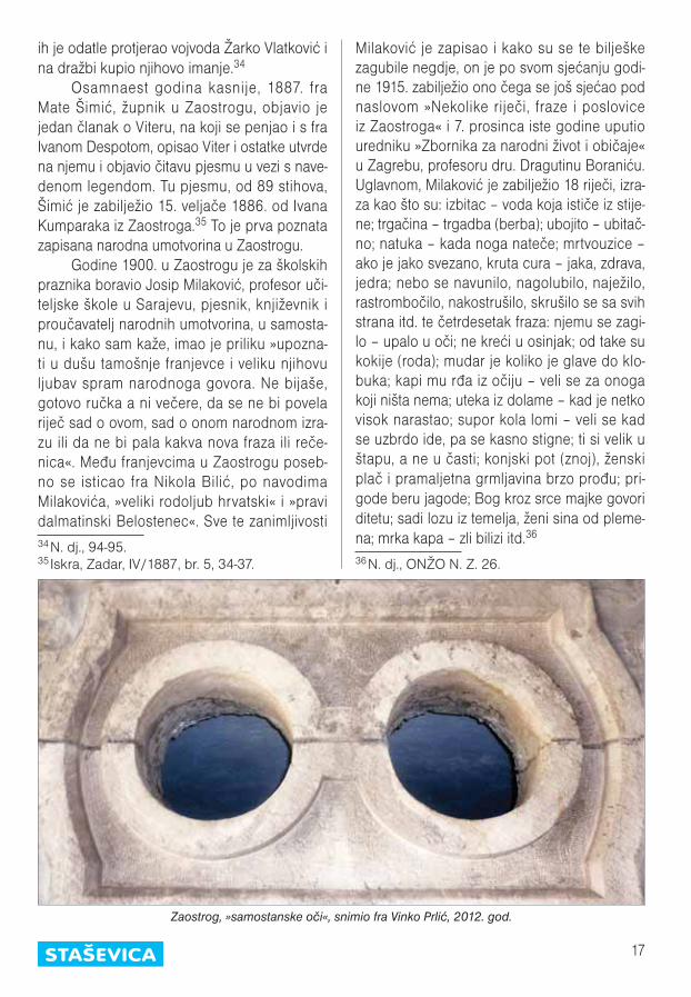
over a broad range of conditions. The model's performance was verified by comparison of

simulation results with experimental data. When provided the suction refrigerant state,

discharge refrigerant pressure, compressor speed and ambient air temperature, the model

proved capable of predicting the discharge refrigerant enthalpy, the required compressor power

and the refrigerant mass flow rate with reasonable accuracy.

iii

Table of Contents

Chapter Page

Nomenclature ............................................................................................. vi

1. Introduction and Objectives ......................................................................... 1

2. Literature Review .................................................................................... 4 2.1. Introduction ................................................................................. 4 2.2. Research ..................................................................................... 4 2.3. Conclusions ................................................................................ 12

3. Analytical Equation Development ................................................................. 14 3. 1. Introduction ....................................................... : ........................ 14 3.2. General Model Description ............................................................. 14 3.3. Compressor Capacity ..................................................................... 16 3.4. Power ....................................................................................... 21 3.5. Discharge State ............................................................................ 23

4. Experimental Procedure and Data ................................................................. 26 4.1. Introduction ................................................................................ 26 4.2. Facilities Outline ........................................................................... 26 4.3. Experimental Procedure .................................................................. 28 4.4. Experimental Results ..................................................................... 30 4.5. Additional Calculations ................................................................... 33

5. Empirical Equation Development and Parameter Estimation Using Least Squares Methods ..................................................................... 41

5.1. Introduction ................................................................................ 41 5.2 Isentropic Volumetric Efficiency ....................................................... .41 5.3 Isentropic Work Efficiency ............................................................ .45 5.4 Compressor Heat Loss ................................................................... 49

6. Steady-State Compressor Model Equations and Results ....................................... 54 6.1 Introduction ........................ '" .......................................... , . " ....... 54 6.2 Model Equations and Solutions .......................................................... 54 6.3 Steady-State Model Performance ....................................... " ............... 57

7. Conclusions and Recommendations .............................. " .............................. 60 7.1 Conclusions ......................... " ..................................................... 60 7.2 Recommendations ......................................................................... 61

References ................................................................................................ 63

Appendix A. Experimental Facility ................................................................. 66

Appendix B. Multi-Variable Linear Least-Squares Analysis Program ......... '" .............. 70

Appendix C. Refrigerant Properties ................................................................ 74

Appendix D. Turbine Flow Meter Calibration ...................................................... 76

v

Nomenclature

hs Suction Refrigerant Specific Enthalpy

h<t Discharge Refrigerant Specific Enthalpy

h<t-s Discharge Refrigerant Specific Enthalpy at Constant Entropy

L\h Enthalpy Rise Across the Compressor

Ih Refrigerant Mass Flow Rate

N Compressor Speed

Ps Suction Refrigerant Pressure

Pd Discharge Refrigerant Pressure

Q,hell Compressor Heat Loss

r Clearance Fraction

Ss Suction Refrigerant Specific Entropy

Ta Ambient Air Temperature Surrounding the Compressor

Te Representative Compressor Shell Temperature

UA Overall Heat Transfer Coefficient

Vs Suction Refrigerant Specific Volume

Vd-s Discharge Refrigerant Specific Volume at Constant Entropy

V cl Clearance Volume

V disp Compressor Displacement

V s Suction Stroke Refrigerant Volume

V s Suction Refrigerant Volumetric Flow Rate

V s-s Isentropic Suction Refrigerant Volumetric Flow Rate

We Work of Compression

We-s Isentropic Work of Compression

We Compressor Power

1lel Clearance Volumetric Efficiency

vi

Nomenclature Continued

11v-s Isentropic Volumetric Efficiency

11w-s Isentropic Work Efficiency

t Jackshaft Torque

vii

Chapter 1

Introduction and Objectives

Historically, much of the automotive air conditioning industry has been dominated by

chlorofluorocarbon (CFC) refrigerants, particularly R-12 (dichlorodifluoromethane).

However, CFC refrigerants are suspected of causing harm to the environment. They are

believed to be partially responsible for the depletion of the earth's ozone layer. Therefore, due

to this concern, there has been a recent effort to find alternative refrigerants to CFC's.

One replacement candidate for R-12 is R-134a (1,1,1,2-tetrafluoroethane). However,

R-134a cannot simply be used to replace R-12 in existing systems. R-12 and R-134a possess

different thermodynamic and physical properties in addition to different lubricant and material

compatibilities. Many design changes must be incorporated to bring the performance and

efficiency of new R-134a systems up to those of past R-12 systems. Furthermore, with the

increased use of microprocessors in automobiles, additional improvements in air conditioning

system performance can be achieved through the use of optimal or adaptive control algorithms.

To facilitate design changes, aid in system performance optimization and allow for the

development of advanced control algorithms, reasonably accurate mobile air conditioning

system models need to be developed.

If a mobile air conditioning model is to be useful, it must simulate the system under

transient conditions. Mobile air conditioning systems almost always operate under transient

conditions. These transients are primarily induced by changes in the compressor speed

(proportional to engine speed), changes in the inlet air conditions of the evaporator and

condenser, and cycling of the compressor to avoid evaporator frosting. To facilitate the

1

development of transient simulation models, it is often useful to start with the development of a

steady-state model.

The present study is a segment of a mobile air conditioning transient modeling

investigation being conducted by the Air Conditioning and Refrigeration Center (ACRC) at the

University of lllinois at Urbana-Champaign. The transient system model under development is

based on simple analytical equation forms derived from basic conservation of mass, energy,

and momentum equations. This helps maintain a reasonable system simulation time by

avoiding the complexities of a finite element approach. In addition, the final model equations

will contain physical system parameters such as the compressor displacement and condenser

area in addition to parameters estimated from experimental data.

By varying the physical parameters within the system model, system performance

optimization can be performed without the use of exhaustive experimental efforts.

Furthermore, by analyzing the effect of each system parameter on overall system performance,

potential improvements to system components can be prioritized. This prioritization can

indicate which areas of mobile air conditioning research will provide the greatest increase in

system performance. This will aid in the difficult task of deciding where to devote research

efforts. In addition, the system model can be used to analyze and develop optimal and adaptive

system control algorithms for increased transient system performance.

Since the system model equations contain parameters based on experimental data, the

specific model developed is system dependent. However, more important than the numbers

from the current system model is the modeling algorithm presented. The equation forms

should be valid, independent of the system. Only the parameter magnitudes will change from

system to system. Hopefully, the algorithm used to develop the current model can easily be

2

applied to a wide variety of systems with a minimal amount of experimental data for parameter

estimation.

The complete system model under development is composed of individual component

models which are each developed separately. The objective of the current study is to develop a

modeling algorithm for an automotive air conditioning compressor. The compressor model

development follows all of the system model guidelines outlined above. To facilitate the

development of a transient compressor model, a steady-state model is developed ftrst. This

report contains details concerning the development of a steady-state compressor model with

suggestions provided for future development of a transient form.

The experimental data required for parameter estimation and model veriftcation are

provided by a mobile air conditioning test facility utilizing R-134a as the working refrigerant.

Relevant details of the experimental facility and the experimental procedure in addition to the

experimental data are presented within this report.

3

Chapter 2

Literature Review

2.1 Introduction

A great deal of literature exists on the steady-state and transient analysis of vapor­

compression cycles. However, there is little work involving automotive air conditioning

applications. The goal of the present study is to develop a steady-state compressor model for

use in a complete system simulation. It is expected that the completed steady-state model will

be extended to develop a transient version. Since little research has been done in this area,

insight from similar works involving different system simulations will be investigated.

2.2 Research

Cecchini and Marchal (1991) developed a general steady-state system simulation model

based on experimental data. They attempted to develop component models in which the

component could be characterized by a small number of parameters estimated from a few

experimental data points. The compressor model utilized a polytropic-based expression for

predicting the discharge refrigerant state similar in form to the reversible polytropic work of

compression. The polytropic exponent was defined as an input parameter to the model. The

steady-state refrigerant mass flow rate was estimated using an equation based on the pressure

ratio and polytropic exponent with the compressor displacement and the clearance fraction as

equation parameters. Although the model accounted for different compressor geometries, none

of the model equations contained a reference to the compressor speed. It was unclear what

assumptions were made about heat loss from the compressor and how the compressor power

was determined. No details concerning the development of the compressor model equations

4

were provided. The system model was verified through the use of experimental data. For an

air-to-air system, the model was able to predict the compressor power within ± 10%.

Furthermore, when the model was used to simulate an air-to-water heat pump, the compressor

power was predicted to within ± 7%.

Chi and Didion (1982) presented a simulation model of a heat pump. The heat pump

utilized a hermetic reciprocating compressor. The model equations were developed using a

polytropic approach. A simulation of a 4-ton residential air-to-air heat pump operating in the

cooling mode was performed with R-22 as the working fluid. The simulated start-up transients

were compared to experimental data. The predicted results compared reasonably well with the

simulated results .

Davis and Scott (1972) proposed a simulation of an automotive air conditioning system

in conjunction with a vehicle compartment simulation. The model simulated an automotive

type reciprocating compressor and predicted the refrigerant discharge state and the shaft work.

The refrigerant mass flow rate was defined as an input parameter to the compressor model and

was determined by a thermostatic expansion valve model in the system simulation. The

compressor was modeled as isentropic using ideal gas relationships. In addition, a refrigerant

leakage coefficient, and the mechanical efficiency were designated as input parameters to the

model. The compressor model also accounted for work done in the suction and discharge

valves by relating the work to the associated pressure drops empirically. The suction valve

pressure drop was estimated as a fraction of the total suction pressure and the discharge valve

pressure drop was estimated from an ideal gas relation. The model did not account for

differences in compressor size or speed. In addition, no experimental verification or simulation

results were presented.

5

Davis and Scott (1976) outlined a hermetic compressor model for use in a system

simulation. The steady-state compressor model included heat transfer within the compressor

shell and pressure drop in the suction and discharge passages. In addition, the model included

the electric motor dynamics and allowed for the modeling of different compressor sizes and

speeds. The model required that the mechanical and volumetric efficiencies specified as input

parameters. These parameters were to be determined from experimental data. No experimental

verification or simulation results were presented.

Dhar and Sodel (1979) discussed a vapor-compression system simulation model

utilizing a hermetically sealed reciprocating compressor. They assumed that the compression

process is polytropic, that the compressor operates at a constant speed, and that the pressure

drop in the suction and discharge valves is negligible. Although no equations were given, they

claimed that the refrigerant mass flow rate and the work done by the compressor on the

refrigerant could "easily be derived as a function of compressor geometry, suction and

discharge pressure ratios, refrigerant leakage rate, compressor speed and the specific heat ratio

of the refrigerant." The discharge state refrigerant enthalpy was determined by adding the

work done by the compressor on the refrigerant to the suction refrigerant enthalpy. Then, an

overall efficiency was used to determine the rate of energy released from the compressor due to

friction and other losses in addition to the work input to the compressor. The model also

included calculations of the internal heat transfers within the compressor shell. Furthermore,

the model included a detailed analysis of the oil-refrigerant interaction in the compressor sump.

Refrigerant property calculations were performed using curve fits of refrigerant property tables.

In Part II of the paper, simulation results of the start-up transient for a window air conditioner

were presented. No experimental verification was provided.

Domanski and McLinden (1990) outlined a rudimentary steady-state compressor model

included as part of a generic system simulation model, CYCLEIl. The compressor model

6

provided three options: an isentropic compressor, a polytropic compressor and a hennetic

polytropic compressor including internal heat transfer and volumetric efficiency. The heat

transfer equations for the hennetic compressor were based on simple energy balances with heat

transfer coefficients based on Prandtl and Reynolds Number correlations. The refrigerant state

after compression was determined from the reversible polytropic work of compression and a

user defined polytropic efficiency. The polytropic efficiency was defined as the ratio of the

polytropic work of compression to the energy transferred to the refrigerant during

compression. The polytropic exponent was defined using the polytropic efficiency and the

isentropic index, 'Y. The isentropic index was determined from an ideal gas relationship instead

of the ratio of specific heat capacities. Domanski and McLinden chose a polytropic process

rather than an isentropic process for simulations claiming that the polytropic efficiency was

more constant than the isentropic efficiency which varies with pressure ratio. The volumetric

efficiency was detennined from an equation based on the pressure ratio and polytropic

exponent with constant "experience factors" included for leakage and clearance volume effects.

No equation was provided for predicting the overall power input to the compressor which was

composed of power transferred to the refrigerant and heat loss. In addition~ the model

provided no provisions for different compressor speeds or sizes. Furthennore, no

experimental verification was provided, only simulation results comparing the perfonnance of

different refrigerants.

Ellison et al. (1979) presented an overview of the Oak Ridge National Heat Pump

Model. This model simulates the steady-state perfonnance of a hennetic compressor operating

at a constant speed. The model required perfonnance and efficiency parameters as well as heat

transfer infonnation obtained from experimental data as input parameters. Tables were.

presented comparing a few experimental points with simulation results.

7

Hai and Squarer (1974) presented a detailed model for simulating multi-cylinder

reciprocating compressors. The governing differential equations were developed from ideal

gas relationships and were based on incremental changes in the crankshaft angle. In addition,

the model used differential equations to model the valve dynamics throughout the compression

cycle. The model equations were capable of predicting the compressor torque in addition to

refrigerant mass flow rate. However, there was no prediction of the discharge refrigerant state.

The compression cycle was simulated for a constant compressor speed. The cycle averages

were compared to three experimental data points. The refrigerant mass flow rate corresponded

reasonably well with the experimental data. However, the predicted cycle average torque did

not compare as favorably.

James and James (1986) provided a transient model of a heat pump utilizing a water

cooled hermetic compressor operating at a constant speed. To model the internal heat transfers,

the compressor was divided into zones. A mass and energy balance was then used on each

zone. However, the actual compression cylinder was assumed to be only one zone.

Furthermore, many of the internal heat transfers were ignored. The internal heat transfers that

were modeled were complicated by the lack of heat transfer coefficients. The refrigerant mass

flow rate through the compressor was determined using a constant volumetric efficiency which

was a model input parameter. James and James expressed an interest in relating this efficiency

to pressure ratio at a later date. The work of compression was determined using an integration

of the polytropic process. The polytropic exponent was designated as a model input parameter.

Since no polytropic efficiency was used, the polytropic equation provided only the reversible

work done on the refrigerant. The predicted work of compression does not include frictional

and other losses within the compressor. In addition, it was assumed that there was no net heat

loss from the compressor. Therefore, a simple energy balance was used to predict the

discharge refrigerant state. The only transient equations provided involved the internal heat

transfer equations. These transients were due solely to the thermal capacities of the compressor

8

components. No experimental verification of the model's performance was provided.

However, a computer code listing of the system model program was included.

MacArthur (1984) modeled a hermetic compressor for use in a heat pump in great

detail. The transient model was based on an energy balance on the compressor cylinder and

included the throttling process of the refrigerant passing through the suction and discharge

valves. The model also considered the heat transfer to the cylinder walls and the thermal

capacity of the compressor components. The compression process was assumed to be

polytropic. The input parameters to the model included compressor displacement, clearance

factor, compression efficiency, heat transfer coefficients and thermal masses. Simulation

results for the steady-state refrigerant mass flow rate in addition to the transient response of the

discharge refrigerant temperature and mass flow rate during start-up were presented. No

experimental verification was provided.

Murphy and Goldschmidt (1985) perfonned a study of the start-up transients found in a

residential air conditioner. Although the objective was to model start-up transients, the

constant speed hermetic compressor was modeled using steady-state equations. To account for

friction and other losses in the compressor power detennination, a modified form of a power

equation for an ideal compressor was used. The resulting expression for compressor power

was a linear function of only the suction and discharge refrigerant pressures. A least squares

analysis was used to detennine the equation constants. In a similar manner, the refrigerant

mass flow rate was expressed as a function of the refrigerant pressure ratio and the suction

refrigerant density. Again, the equation constants were obtained from a least squares analysis.

When the compressor power was simulated under system start up, the predicted power was

observed to follow the same trends as the experimentally measured values. However, the

predicted power was significantly lower than the experimental values although the steady-state

values were the same. This indicates that there are other significant transient factors besides the

9

refrigerant suction and discharge pressures which influence the compressor power. Murphy

and Goldschmidt offered two explanations for this discrepancy between the predicted and

experimental values. First, during start up, the oil could foam and cause increased flow

resistance through the compressor. Second, there is additional superheating of the suction

refrigerant in the hermetic compressor shell due to the initially hot components within the shell.

This additional superheat would not appear in the experimentally measured suction pressure.

This is a likely explanation since the internal heat transfer within the compressor shell was

ignored in the model. The authors concluded that steady-state compressor models used for

quasi steady-state transient simulations provide good trends during start up, but provide poor

qualitative numbers.

Prakash and Sing (1974) presented a detailed model of an open reciprocating

compressor where events taking place in the compression cylinder were linked to incremental

changes in the crank shaft angle. Ideal gas relations were used to develop time dependent

differential equations for each part of the compression process. The model equations ignored

all work loss to friction. Correlations extracted from the literature were utilized to model the

the heat transfer within the compression cylinder. No simulation results or verification were

provided.

Sami et al. (1987) presented a model for simulating the dynamic response of heat

pumps. A reciprocating compressor was modeled using time dependent differential equations

derived from ideal gas relations. All time derivative terms of the compressor model involved

refrigerant mass, refrigerant pressure and piston displacement. No transients due to thermal

capacities were included. The model included equations for refrigerant pressure drop as it

passes through the suction and discharge valves. In addition, since the model equations

contained terms with areas and piston displacement rates, different size compressors and

different compressor speeds could be simulated. No attempts were made to model the internal

10

heat transfer of the compressor. The net heat loss from the compressor was modeled with a

simple temperature differential approach with a heat transfer coefficient determined from an

existing correlation. The model also included refrigerant property calculations which accounted

for the effects of oil on the thermodynamic properties of R-12 and R-22. A quasi steady-state

transient simulation of a vapor-compression refrigerating system was performed and compared

to the simulations of Yasuda et al. (1982). The predicted compressor power agreed

reasonably well between the two simulations. In addition, the start-up transients were

compared to the experimental data found in Hamel (1982). The predicted compressor

refrigerant discharge temperature deviated from the experimental values during the start-up

transients. However, the discharge temperature agreed reasonably well with the experimental

values at steady state. The predicted refrigerant discharge pressure agreed with the

experimental data in both the transient and steady-state portions of the simulation. No other

comparisons directly involving the compressor were given. Based on the presence of the

piston displacement derivative in the governing equations, it is believed that the solution time

step would be rather small. This may lead to extremely long computational times for a

reasonable length simulation. No indication of computational time requirements were

presented.

Sami and Duong (1991) extended the system simulation model of Sami et al. (1987) by

incorporating changes to the heat exchanger models. The compressor model remained the

same. However, this time a water-to-water heat pump was simulated using R-134a and R-12

as the working fluids. The refrigerant property calculations were performed for pure

refrigerant only. The equations of state were formulated by McLinden et al. (1990) using a

modified Benidict-Webb-Rubin equation of state. The steady-state performance of the model

was verified with experimental data for a three-ton water-to-water heat pump operating in the

heating mode. Although the heat pump contained a variable speed compressor, the

experimental data was recorded with the compressor operating at a constant speed. The

11

predicted steady-state system capacity agrees well with the experimental values for R-134a In

addition, the predicted steady-state COP agrees with the experimental values within ±5% for

both R-134a and R-12. This indicates that the compressor model is independent of the

refrigerant used. Quasi steady-state simulations of start-up transients were performed for both

R-12 and R-134a. The transient performance of both refrigerants were compared graphically.

2.3 Conclusions

There are many fundamental differences between the majority of the compressor

models reviewed in this chapter and the requirements of the present study. Most of the

research reviewed is concerned with the modeling of hermetic compressors for heat pump

applications. When modeling hermetic compressors, it is essential that the heat transfer

occurring between the motor and the oil, in addition to the refrigerant and other components

within the compressor shell, are accounted for. For most of the models reviewed, a great deal

of the modeling effort was dedicated to modeling these heat transfers. However, the current

study involves an open compressor where the internal heat transfers may not hold as much

importance and therefore may require a much different model form. In addition, many of the

compressors modeled contained only a single cylinder. The compressor of the present study

contains ten (five double-acting) compression cylinders. Again, this may affect the model

equation forms. Furthermore, the compressor used in the present study can be operated over a

wide range of compressor speeds. However, many of the models reviewed simulated the

compressor at a constant speed. It is believed that the compressor speed has a strong effect on

the compressor performance. Therefore, it is suspected that the accuracy of many of the

models presented would suffer greatly if the simulation results were compared to experimental

data for a range of compressor speeds.

12

Several of the papers reviewed contained studies of system start-up transients. In

these transient investigations, the compressor speed is set and all other external system input

variables remain constant These studies are concerned chiefly with refrigerant migration. In

contrast, one of the long term goals of the present study is to simulate transients during the

normal operation of the air conditioning system. These transients would be induced by

changes in the inlet air conditions of the heat exchangers or dynamic changes of compressor

speed The changes of heat exchanger inlet air conditions would result in dynamic changes of

the suction or discharge refrigerant states and thus lead to compressor dynamics. These

compressor dynamics are vastly different than those encountered during system start-up.

Other reviewed research modeled the transient behavior of the compressor using an

incremental crankshaft angel approach. However, this does not appear to be a practical

approach for the current study. Events occurring in the compression cylinders are relatively

fast. When these events are compared to the behavior of the complete system, it can be

assumed that they occur instantaneously. Therefore, such mathematical detail is unnecessary

when the compressor model is part of a system simulation. This type of detailed analysis

would lead to excessive computational times for a reasonable length system simulation.

Finally, it was observed that almost all of the compressor simulations presented

required information obtained from experimental data. In addition, many of the simulations

presented lacked experimental verification.

13

Chapter 3

Analytical Equation Development

3.1 Introduction

The general requirements of the steady-state compressor model are outlined in this

chapter. The input and output requirements of the model are established. Furthermore, the

development of steady-state compressor model equations and relations are described within this

chapter. Basic analytical equations or empirical modeling strategies are derived for predicting

the refrigerant mass flow rate, required compressor power, and the discharge refrigerant

enthalpy as functions of specified input variables and parameters.

3.2 General Model Description

The compressor used in the current study is a multi-cylinder, swash-plate, reciprocating

compressor with reed valves on the suction and discharge ports (See Appendix A). However,

for modeling purposes, the compressor will be treated as a single-cylinder reciprocating

compressor with characteristics equivalent to the sum of the multiple cylinders. Furthermore,

the model will explicitly ignore the compressor's internal geometry (valve passages, etc.)

except for the compression cylinder volumes.

Before equations can be developed, the desired input and output relationship of

variables and model parameters must be established. The model schematic found in Figure 3.1

illustrates the input and output relationship of the parameters and variables for the steady-state

compressor model. The model input variables are

Ps = suction refrigerant pressure,

14

Input

hs = suction refrigerant specific enthalpy,

Pd = discharge refrigerant pressure,

N = compressor speed,

Ta = ambient air temperature surrounding the compressor.

Physical Empirical Parameters Parameters

'Xtisp Vel Cl, C2, •••

! ! ! ! Ps ~

hs ~ Variables ~ ~

N .-Ta .-

'-m OUtput

.-W Variables e

.-hd

Figure 3.1. Steady-State Compressor Model Input and Output Relationships

The model output variables are

Ih = steady-state refrigerant mass flow rate,

Vic = compressor power,

hd = discharge refrigerant specific enthalpy.

In addition, there are two input physical (geometric) parameters

V disp = compressor displacement or suction stroke swept volume,

V cl = clearance volume.

The model also requires the input of empirical parameters estimated from experimental data.

These parameters are discussed in later chapters.

15

Enthalpy is utilized in conjunction with pressure to define the suction and discharge

refrigerant states. Enthalpy is chosen because it is always independent of refrigerant phase.

This is important when specifying suction refrigerant states that are near saturation. Once the

pressure and enthalpy are known, simple thermodynamic relationships can be used to

determine other state variables such as temperature and specific volume.

Note that to predict IiI, the steady-state compressor model requires the knowledge of the

discharge refrigerant pressure. The compressor must know the pressure at which its

compressed refrigerant is discharged. This has a direct bearing on the compressor capacity as

well as the required compressor power. Even if the compressor model were simplified to the

case of an ideal isentropic compression process, the discharge refrigerant pressure would have

to be known to determine the outlet state and would obviously affect the isentropic work of

compression.

The steady-state compressor model consists of three basic submodels: capacity,

power, and discharge state. Each submodel can be solved sequentially starting with capacity.

The capacity model predicts refrigerant mass flow rate. The power model is used to predict the

required compressor power. Finally, the discharge state model estimates the refrigerant

discharge enthalpy.

3.3 Compressor Capacity

The compressor capacity component of the model is utilized to predict the steady-state

refrigerant mass flow rate through the compressor. The general modeling approach is to define

an isentropic volumetric efficiency. From this relation, the actual suction refrigerant

volumetric flow rate and thus the refrigerant mass flow rate can be predicted.

16

Before an isentropic volumetric efficiency is defined, the characteristics of an ideal

isentropic compressor should be discussed. An ideal isentropic process is one that is both

adiabatic and reversible. For an ideal isentropic compressor, given the suction refrigerant state

and the discharge pressure, the discharge refrigerant state is defined by the entropy of the

suction state and the discharge pressure. There is no heat transfer between the refrigerant and

the ambient. In addition, there are no irreversibilities such as pressure drop across the suction

or discharge valves and mechanical friction.

For an isentropic reciprocating compressor, the isentropic suction volumetric flow rate

can be written as

v s-s = 'Tlcl N V disp (3.1)

where 'Tlcl is the clearance volumetric efficiency for an isentropic compressor as defined in

Stoecker and Jones (1986, pp. 208).

The clearance volumetric efficiency depends only upon the isentropic re-expansion of

the gas trapped in the clearance volume after the piston discharge stroke. It ignores such

effects as suction and discharge valve pressure drop, heating of the suction refrigerant from the

compressor walls and other factors affecting the actual volumetric flow rate.

An expression for the clearance volumetric efficiency of a reciprocating compressor can

easily be derived from the pressure-volume diagram found in Figure 3.2. This derivation

assumes that the cylinder's suction and discharge ports are regulated by simple pressure

activated valves such as reed valves. In Figure 3.2, V m is the maximum volume in the

compression cylinder when the piston is at the bottom of its stroke. The clearance volume,

V ct. is the minimum volume in the cylinder which occurs when the piston is at the top of its

stroke. When the piston is at the top of its stroke, there will be a small amount of gas trapped

in the clearance volume which was not discharged in the previous cycle. This gas is at the

17

discharge pressure, Pd. As the piston moves downward, the gas trapped in the clearance

volume expands until its pressure is equal to the suction line pressure, Ps. This corresponds to

Pressure

Volume

Piston ••••

Figure 3.2. Pressure-Volume Relationship For an Isentropic Compressor

a cylinder volume Vi. As the cylinder volume increases further, the suction valve opens,

drawing refrigerant into the cylinder until the end of the suction stroke. The piston then

reverses direction, decreasing the cylinder volume and compressing the refrigerant. When the

compressed refrigerant reaches the discharge pressure, the discharge valve opens and the

refrigerant is discharged from the cylinder during the remainder of the stroke.

18

Since the compressor is assumed to be ideal, no thermodynamic work occurs in the

portions of the cycle where the discharge or suction valves are open and refrigerant is being

discharged or drawn into the cylinder. This is a result of both the refrigerant pressure and

specific volume remaining constant. As a result, the compression stroke is an isentropic

process in addition to the suction stroke.

The volume of gas moved through the compressor for each stroke of the piston is V s.

The clearance volumetric efficiency can then be expressed as

Vs Vrn - Vi 111----c -Vdisp - Vrn - Vcl (3.2)

The clearance fraction is defined as

_ Vel Vel r - ---

- Vdisp - Vrn - Vcl (3.3)

Equation 3.2 can be combined with Equation 3.3 and rearranged algebraically to a more

common form:

y l1cl = 1 - r (" 1 - 1)

vel

Note that the clearance fraction is simply a geometric property of the compressor.

(3.4)

Since the mass of refrigerant contained in Vcl is the same as that contained in Vi, and it

is assumed that the expansion of the clearance volume refrigerant is isentropic, then

(3.5)

19

where v s is the suction refrigerant specific volume and v d-s is the discharge refrigerant specific

volume at the suction entropy and the discharge pressure. Therefore, the clearance volumetric

efficiency of an ideal isentropic compressor is

Vs llcl = 1 - r (- - 1)

vd-s (3.6)

The two specific volumes, v s and v dos, can be determined from the model input variables with

the simple thermodynamic relationships

Vs = f(Ps,hs)

Ss = f (P s,hs)

vd-s = f(Pd,Ss)

where Ss is the suction refrigerant entropy.

(3.7)

(3.8)

(3.9)

For a real compressor, the actual volumetric flow rate will be less than the

corresponding isentropic volumetric flow rate for a given operating point. The most important

factors affecting this difference typically include suction and discharge valve pressure drop,

valve and piston ring leakage, and cylinder wall and compressor port heat transfer with the

suction and discharge refrigerant. Furthermore, one would expect the volumetric efficiency of

a real compressor to have a dependence upon compressor speed due to fluid acceleration effects

and cross correlations to compressor pressure ratios, piston ring leakage, and valve pressure

drops. This is most important in automotive compressor applications where the compressor

encounters a wide and varying range of speeds.

To predict the actual volumetric flow rate, an isentropic volumetric efficiency is defmed

as

_ Vs llv-s = -.-

Vs-s (3.10)

20

· . where V s is the actual suction volumetric flow rate and V s-s is the suction volumetric flow rate

of an ideal isentropic compressor operating at the same speed, suction refrigerant state, ambient

temperature and discharge pressure. The dimensionless variable l1v-s accounts for the

differences between the actual volumetric efficiency and the clearance volumetric efficiency

mentioned above.

It is desired to use Equation 3.10 to predict V s for the compressor. With the given

input variables and parameters, V s-s can easily be determined from the equations given above.

However, an analytical expression for l1v-s is difficult to obtain. Therefore, a functional

relationship of 11 v-s to other model variables should be determined empirically from

experimental data and will be addressed in later chapters.

If the suction refrigerant volumetric flow rate is known, the steady-state refrigerant

mass flow rate can be predicted. The refrigerant mass flow rate through the compressor can be

determined from the suction volumetric flow rate and the suction specific volume as follows:

(3.11)

3.4 Power

The required power input to the compressor can be predicted from the power model.

The work of compression is predicted through the use of an isentropic work efficiency

approach. Then, the predicted work of compression is combined with the capacity model to

predict the compressor power.

21

The isentropic work of compression is defined as the required work per unit mass to

compress the refrigerant from the given suction refrigerant state to the specified discharge

pressure with an ideal isentropic process. The isentropic work of compression can be written

as

we-s = hd-s - hs (3.12)

where hs is the suction refrigerant enthalpy and hd-s is the discharge refrigerant enthalpy at

constant entropy calculated from the thermodynamic relation

(3.13)

An isentropic compression process is both adiabatic and reversible. However, the

actual compression process contains both heat transfer and irreversibilities. To account for the

difference between the actual and the isentropic work of compression, a dimensionless

isentropic work efficiency is defined as

_ We-s l1w-s = We

where We is the actual work of compression.

(3.14)

To utilize Equation 3.14 to predict the actual work of compression from the isentropic

work of compression, the efficiency needs to be known. One would not expect the isentropic

work efficiency to be a constant as is sometimes assumed in the literature. Instead, one would

expect the isentropic work efficiency to have a functional relationship to system variables that

relate to compressor irreversibilities. These irreversibilities typically arise from mechanical

friction, internal heat transfer, and fluid friction (pressure drop). The functional dependence

of l1w-s on the other model variables can be determined from experimental data and will be

addressed in later chapters.

22

If the work of compression is known, the capacity model can be used to predict the

required compressor power. This can be expressed as

(3.15)

3.5 Discharge State

The steady-state compressor model must be able to predict the refrigerant discharge

state. Since the discharge pressure is an input variable, the discharge refrigerant enthalpy must

be determined. Figure 3.3 shows a control volume around the compressor upon which the

First Law of Thermodynamics can be imposed. This results in an expression for the discharge

refrigerant enthalpy,

h<t = We -. Oshell + hs m

where Oshell is the heat loss rate from the compressor shell to the ambient.

Control Volume

~\-~hell

..

J

Figure 3.3. Control Volume For Energy Analysis

(3.16)

To utilize Equation 3.16 in predicting the refrigerant discharge enthalpy, the

compressor shell heat loss rate must be predicted. However, the compressor shell heat loss is

23

a complicated variable to predict. There are many possible energy transfer paths within the

compressor which complicate modeling attempts. Figure 3.4 provides a simplified flow

diagram for some of the possible energy transfer paths through the compressor. This

simplified schematic lumps the compressor system into two control volumes, the compressor

and the refrigerant. The compressor control volume consists of all the physical parts (housing,

cylinders, swash plate, etc.) of the compressor and the refrigerant control volume is simply the

refrigerant traveling through the compressor. The power input to the compressor is split

between the two control volumes. There is a component generating heat in the compressor and

a component transferring work to the refrigerant. The split of this energy transfer is unknown.

Furthermore, there is heat transfer between the compressor and the suction and discharge

refrigerants. In addition, since there may be thermal gradients within the compressor control

volume, there will be heat transfer from one part of the control volume to another. Similarly,

there is energy entering the refrigerant control volume with the incoming refrigerant. After

exchanging heat with the compressor control volume and receiving a portion of the input

power, the resulting net energy is carried out of the refrigerant control volume with the

refrigerant stream. Finally, there is a heat loss from the compressor control volume to the

ambient.

The difficulty in modeling the compressor shell heat loss lies in ·the

determination of the dominant energy transfer paths of which the compressor shell heat loss is

composed. Unfortunately, there are more energy transfers than there are control volumes and

thus the heat transfer paths cannot be determined analytically from conservation of energy. In

addition, the internal heat transfer quantities cannot be measured directly and the heat transfer

paths cannot be accurately determined experimentally. Therefore, the dominant heat transfer

paths can only be estimated from the experimental data. This analysis will be addressed in a

later chapter. However, some expected trends can be discussed. First, it is possible that the

energy transfer to the compressor control volume from the input power is dominated by friction

24

and would therefore have a strong dependence on compressor speed. Furthermore, if the

dominant heat transfer path is from the frictional heat generation to the ambient, then one would

expect the compressor shell heat loss rate to be independent of the ambient temperature and

only depend upon frictional terms such as compressor speed. If it is assumed that the

compressor control volume is at a constant temperature, only the compressor control volume

temperature should vary, but not the heat transfer rate. In contrast, if the compressor shell heat

loss is dominated by refrigerant-compressor heat transfer, then the compressor heat loss rate

would depend on the ambient temperature (ignoring heat conducted from the compressor by its

supports). A equation form of

flshell = VA L\ T (3.17)

would be expected. The L\ T term would be a temperature difference between some

representative compressor temperature (a function of refrigerant temperatures perhaps) and the

ambient air temperature while VA would be the overall heat transfer coefficient.

Suction Refrigerant

Discharge

Figure 3.4. Simplified Compressor Energy Transfer Path Schematic

25

Chapter 4

Experimental Procedure and Data

4.1 Introduction

This chapter contains a brief outline of the experimental test facility in addition to the

experimental procedure utilized for data acquisition. Tables of experimentally measured

variables are provided. Furthermore, equations for determining additional model variables

from the experimental data and tables of these calculation results are presented.

4.2 Facilities Outline

This section contains a brief outline of the test facility. For a more detailed description,

see Appendix A.

Experimental data were obtained through the use of a mobile air conditioning system

test facility utilizing R-134a as the working refrigerant. The test facility contains an entire

mobile air conditioning system operated with controlled external variables. The condenser and

evaporator are enclosed within air loops where the temperature, humidity and velocity of the air

across the heat exchangers can be controlled. The pressure drop between the condenser and

evaporator is set with a metering valve. In addition, the compressor pulley is driven by a

variable-speed electric motor. This electric motor drives a jackshaft which is coupled to the

compressor through a V -belt and a pair of pulleys. An enclosure of foam board insulation was

constructed around the compressor to provide control over the compressor ambient air

temperature and velocity. The compressor ambient air temperature and velocity are controlled

through the use of a common hair dryer blowing into the compressor enclosure. A manual

26

switch is available to operate the compressor's electromagnetic clutch since the normal pressure

activated switch has been disconnected.

Experimental data were recorded through the use of a computer-based data acquisition

system. The system test facility has a wide variety of instrumentation. Every major

component in the refrigeration loop has pressure and temperature measurements on its

refrigerant inlet and outlet ports. The volumetric air flow rate is measured on both heat

exchanger air loops in addition to temperature and humidity measurements.

N [RPM]

t [in lb]

t Ps [psi]

m [lb/hr] Ts [Of]

Figure 4.1. Schematic of the Compressor With Experimentally Measured Variables

For compressor modeling, eight variables were recorded. Figure 4.1 shows a

schematic of the compressor with the related experimentally measured variables and their units.

The suction and discharge refrigerant pressures, P s and P d, were measured with gauge

pressure transducers on the inlet and outlet ports of the compressor. The atmospheric

pressure, read from a barometer, was added to these pressures to give the absolute refrigerant

pressures. In addition, the suction and discharge refrigerant temperatures, Ts and Td, were

measured with thermocouple probes immersed in the fluid streams. The ambient air

27

temperature surrounding the compressor, Ta, was determined using the average of two

thermocouples located in the compressor enclosure. Furthermore, the steady-state refrigerant

mass flow rate, Ih, was measured with a turbine flow meter located in the liquid line between

the condenser and the expansion valve. The compressor speed, N, was recorded through a

speed transducer located on the jackshaft coupled to the compressor pulley. A correction was

made for the difference in pulley diameters on the compressor and the jackshaft. Furthermore,

the jackshaft is equipped with a torque transducer for measuring the jackshaft torque, t.

4.3 Experimental Procedure

Experimental data were acquired for a wide range of system conditions. This range

included both normal and extreme system operating points. This wide range of data is essential

for the compressor model to be valid over the widest possible range of conditions. The wide

range of data also ensures that the subsequent empirical parameter estimation always involves

interpolation and not extrapolation of the data.

To obtain the desired range of experimental data, there were five independent system

variables that were varied: compressor speed (1000 to 4000 RPM), evaporator airflow rate

(100 to 200 SCFM), condenser airflow rate (500 to 1500 SCFM), metering valve position (4.0

to 10.0) and ambient air temperature and velocity (High and Low Settings). Obviously,

changing compressor speed directly affects the compressor performance. However, the

changes in heat exchanger airflow rates affect the compressor suction and discharge pressures

and temperatures. Varying the expansion valve changes the evaporator refrigerant outlet state

and therefore affects the amount of superheat entering the compressor. In addition, changing

the ambient air conditions of the compressor provides different heat transfer characteristics for

the compressor shell.

28

For steady-state data, the independent system variables were set and the system was

allowed to come to steady state. Once steady-state operation was achieved, system data were

recorded every four seconds for one minute. This group of data (fifteen samples) were

averaged to provide one set of steady-state variables. For a new steady-state condition, the

independent system variables were changed and the system was again allowed to come to

steady state.

Although the independent system variables were varied to achieve the widest possible

range of conditions, there were some restraints on the possible independent variable

combinations. To avoid damage to the compressor, the independent system variables were not

varied in such a way that the compressor discharge state exceeded 400 psig or 250 OF. These

limits were recommended by the compressor manufacturer.

The final model empirical parameters are based on a relatively small set of data (61

steady-state points). However, the variable ranges of the fmal data set are verified by a much

larger set of data (approximately 400 points). The variable ranges of the final data set span the

ranges of the preliminary set. This preliminary data set was acquired over a long period of time

under a wide variety conditions. There are several reasons for basing the model parameters on

the final set of data. First, the majority of the data points in the preliminary data set contained

refrigerant mass flow rates obtained from a condenser energy balance. At the time the data was

recorded, the turbine flow meter had not been accurately calibrated and its readings were

suspect. Therefore, the refrigerant mass flow rate had to be estimated from a condenser energy

balance. However, it is believed that the calibrated turbine flow meter provides a much more

accurate indication of the steady-state refrigerant mass flow rate than the condenser energy

balance. Furthermore, the final set of data was all recorded within one week. It was hoped

that by using data recorded in a small time span, problems with instrumentation drift and

compressor wear could be eliminated. In addition, the relatively small time span would not

29

allow for significant refrigerant or oil leakage and allow for a data set with consistent

refrigerant and oil charge. Since the preliminary data set was consistent with the final data set,

the preliminary data set was utilized for initial model form development prior to acquisition of

the fmal data set. This provided a much larger data base for determining equation forms with

the final equation parameters estimated from the smaller set.

4.4 Experimental Results

Table 4.1 lists the averaged measured variables of the final data set. The data are

grouped into distinct sets identified by the fIrst character of the test number. Within these sets,

compressor speed is the only independent system variable that was varied. The states of the

other four independent system variables for each group of data are indicated in Table 4.2. Note

that these variables are not listed in Table 4.1 since they do not directly indicate compressor

performance and are not used in the model development. Instead, their net influence on the

compressor is characterized by the measured variables found within Table 4.1.

Table 4.1 Experimental Data

Test Ps Ts Pd Td Ta Ih 't N

Number psia OF psia OF OF lb/hr inlb RPM

A-I 47.0 47.5 200.0 150.5 122.7 263.6 154.7 997.3

A-2 40.2 42.6 225.0 174.3 125.1 305.3 154.3 1499.3

A-3 36.6 39.3 243.8 191.4 126.0 334.0 148.0 2007.0

A-4 34.5 37.5 261.3 199.3 126.1 352.4 142.9 2497.4

A-5 33.1 35.5 275.5 215.1 127.2 367.0 137.3 3004.7

A-6 32.1 33.7 282.7 224.8 127.0 374.8 129.0 3502.7

A-7 31.5 32.5 290.1 232.5 127.8 381.7 122.5 4010.6

30

Table 4.1 Continued

Test Ps Ts Pd Td Ta Ih t N

Number psia of psia of of lb/hr in lb RPM

B-1 49.5 46.9 218.0 154.6 128.8 277.7 162.8 1001.5

B-2 42.6 42.2 249.7 178.1 129.0 322.7 162.8 1495.6

B-3 39.0 39.6 272.9 196.6 128.8 346.2 157.1 1999.9

B-4 36.7 36.8 292.9 202.5 128.3 367.8 151.9 2498.9

B-5 35.5 34.8 308.7 219.1 128.0 380.1 146.0 2997.3

B-6 34.5 32.7 321.0 227.1 129.1 391.7 138.8 3503.7

B-7 34.0 31.1 330.2 233.3 129.3 399.7 132.2 3997.9

c- 1 54.0 48.6 266.5 165.4 128.0 293.0 183.8 984.0

C-2 48.2 43.9 317.3 192.2 129.3 346.4 187.3 1484.4

C- 3 45.2 41.8 356.4 207.3 129.7 377.4 181.6 1990.2

C-4 43.3 40.6 394.2 221.6 130.2 402.8 175.7 2495.5

C- 5 38.4 35.5 351.4 227.1 130.7 401.0 156.1 3000.7

C-6 37.0 33.9 371.1 235.0 130.7 413.1 150.6 3495.5

C-7 36.9 33.9 383.4 241.9 131.2 422.2 142.7 4000.3

D-l 42.9 39.1 180.7 139.0 117.0 227.8 144.9 999.5

D-2 36.2 32.3 202.6 160.7 117.6 268.2 144.5 1504.3

D-3 32.8 27.5 217.0 176.3 117.8 308.8 140.2 2004.9

D-4 30.7 23.9 231.4 181.7 117.8 325.7 134.5 2503.3

D-5 29.5 22.1 239.6 198.3 119.4 336.1 129.9 2999.2

D-6 28.8 19.8 248.3 205.8 118.6 346.0 122.7 3517.0

D-7 28.2 18.7 254.5 213.1 118.9 351.6 116.1 4003.6

E-l 46.1 41.1 199.4 144.9 123.7 260.4 151.6 997.9

E-2 38.7 33.2 222.7 165.6 120.9 301.9 150.4 1513.1

E-3 35.1 28.1 240.2 179.2 121.5 324.1 144.7 2000.1

E-4 33.1 25.2 256.8 187.8 120.9 341.7 138.5 2507.4

E-5 31.8 22.5 269.2 202.5 121.8 355.8 133.2 3004.3

E-6 31.3 21.4 282.8 210.0 121.6 367.7 127.0 3513.1

E-7 30.7 20.5 295.0 217.7 121.4 375.0 121.2 4011.3

F-l 50.0 44.1 246.4 158.2 122.2 274.7 173.9 992.7

F-2 44.5 38.1 292.5 181.9 124.0 328.3 175.3 1492.8

31

Table 4.1 Continued

Test Ps Ts Pd Td Ta m t N

Number psia of psia of of lb/hr in lb RPM

F- 3 41.4 34.4 328.2 194.9 125.2 358.8 169.6 2002.4

F-4 40.2 33.1 363.2 209.8 125.2 384.4 165.1 2502.1

F-5 39.4 31.9 387.5 225.7 126.7 400.3 159.2 3001.7

F-6 34.5 25.4 339.0 221.5 126.7 391.8 138.0 3538.4

F-7 34.0 24.3 349.5 226.0 126.9 399.4 132.1 3998.1

G - 1 39.5 31.5 156.0 123.3 105.6 207.7 134.5 1000.1

G-2 30.5 18.1 190.5 156.7 105.0 277.3 135.2 2005.5

G- 3 27.7 12.1 213.5 178.4 104.7 316.1 127.8 3006.1

G-4 26.6 9.3 226.0 192.6 105.5 345.0 116.7 4002.5

H - 1 36.2 53.1 158.9 156.0 114.8 183.6 127.3 1007.2

H-2 27.2 46.4 186.4 198.2 115.0 227.5 118.5 2013.5

H- 3 24.3 47.8 204.5 229.1 117.1 240.2 109.6 3008.1

1 - 1 40.9 32.4 166.3 137.2 162.5 216.8 133.8 1000.5

1 - 2 30.9 19.9 198.0 169.8 161.8 278.9 129.5 2008.3

1-3 28.3 14.6 219.9 190.1 159.1 315.6 122.0 3004.6

1 - 4 26.7 11.5 233.1 206.1 159.9 333.8 110.2 4004.6

J-l 41.6 33.4 178.3 140.9 164.6 230.6 138.5 1002.2

J-2 33.1 21.1 224.0 169.6 164.8 308.7 136.8 2003.6

J-3 30.3 16.2 254.5 194.5 162.2 341.0 128.2 3014.3

J-4 29.3 13.8 272.6 207.2 161.2 358.3 115.5 4004.1

K- 1 39.7 36.3 169.7 135.7 107.0 215.9 139.7 1009.9

K-2 28.4 23.8 235.8 203.5 117.2 309.4 127.2 3002.0

L-l 42.4 36.5 191.5 140.7 110.2 222.9 149.2 1000.1

L-2 29.7 31.6 279.5 218.6 115.8 303.5 132.8 2990.2

32

Table 4.2 Experimental Data Set Legend

Test Condenser Evaporator Valve Compressor

Set CFM CFM Position Heater

A High High 7.0 Low

B Medium High 7.0 Low

C Low High 7.0 Low

D High Low 7.0 Low

E Medium Low 7.0 Low

F Low Low 7.0 Low

G High High 10.0 Low

H High High 4.0 Low

I High High 7.0 High

J Medium High 7.0 High

K High High 5.0 Low

L Medium High 5.0 Low

4.5 Additional Calculations

In addition to the experimentally measured variables, other experimental variables were

used in the model development. These additional variables were calculated from the eight

measured variables for each steady-state data point

Additional state variables of the suction and discharge refrigerant were determined

using fundamental thermodynamic relationships:

hs = f(Ts,Ps)

Ss = f(Ts,Ps)

Vs = f(Ts,Ps)

33

(4.1)

(4.2)

(4.3)

(4.4)

Occasionally, when the suction refrigerant is very near saturation, the measured temperature

and pressure correspond to a slightly subcooled liquid. In these circumstances, the suction

refrigerant enthalpy, entropy and specific volume were determined from the measured pressure

and an assumed quality of 1.0. State variables for the isentropic discharge refrigerant were

also calculated from fundamental thennodynamic relationships:

vd-s = f(Pd,Ss)

hd-s = f(Pd,Ss)

(4.5)

(4.6)

The thermodynamic functions of Equations 4.1 to 4.6 were evaluated for pure R-134a.

No corrections were made for the effects of oil on the thermodynamic properties of the

refrigerant. For more information concerning the calculation of the refrigerant thermodynamic

properties, see Appendix C.

The required compressor power was calculated using the relation

We = 't N (0.80) (4.7)

where the torque, 't, is the measured compressor drive jackshaft torque. Since the compressor

speed is recorded, the ratio of the pulley diameters, 0.80, must be used to keep the torque and

speed variables consistent. The work of compression was calculated from the compressor

power and the refrigerant mass flow rate:

w. W

_---.C. e - . m (4.8)

The isentropic work of compression and the isentropic work efficiency were calculated from

we-s = hd-s - hs (4.9)

1"1 _ We-s 'IW-S- We

(4.10)

The First Law of Thermodynamics was utilized to calculate the heat loss from the compressor:

(4.11)

34

For the compressor used in the current study

V disp = 10.370 in3

Vel = 0.243 in3

These two values were used to calculate the clearance fraction

r=~=0.0234 vdisp

(4.12)

(4.13)

(4.14)

Using the clearance fraction, the clearance volumetric efficiency was calculated using

1 Vs 'llel = - r (- - 1) Vd-s

(4.15)

Once the clearance volumetric efficiency was determined, the isentropic suction volumetric

flow rate could be calculated from

v s-s = 'llc1 N V disp (4.16)

The actual suction volumetric flow rate was determined from

(4.17)

The isentropic volumetric efficiency was then calculated using

~ 'llv-s = . Vs-s

(4.18)

The results of these calculations can be found in Tables 4.3 and 4.4.

Table 4.3 Calculated Variables I

Test hs I1d Vs Ss vd-s l1d-s We We

Number Btu Btu ft3 Btu ft3 Btu Btu Btu lb lb lb lb R lb lb hr lb

A-I 109.46 124.88 1.030 0.2239 0.250 122.76 4984.2 18.91

A-2 108.96 130.03 1.214 0.2258 0.223 125.02 7472.7 24.47

A- 3 108.55 133.84 1.332 0.2266 0.207 126.30 9593.5 28.72

A-4 108.33 135.26 1.416 0.2273 0.193 127.37 11523.6 32.70

A-5 108.03 139.03 1.470 0.2274 0.183 127.93 13324.0 36.31

35

Table 4.3 Continued

Test hs lld Vs Ss Vd-s lld-s We We

Number Btu Btu ft3 Btu ft3 Btll Btu Btu 1b lb lb lb R lb 1b hr 1b

A-6 107.74 141.41 1.513 0.2274 0.178 128.16 14597.3 38.95

A-7 107.54 143.24 1.538 0.2273 0.172 128.35 15864.0 41.56

B-1 109.16 124.91 0.978 0.2225 0.224 122.71 5264.1 18.96

B-2 108.68 129.85 1.140 0.2242 0.197 125.00 7861.4 24.36

B-3 108.41 133.96 1.245 0.2252 0.181 126.46 10147.7 29.31

B-4 108.02 134.72 1.320 0.2255 0.168 127.29 12256.0 33.32

B-5 107.70 138.77 1.363 0.2255 0.158 127.76 14134.4 37.18

B-6 107.34 140.55 1.396 0.2253 0.151 127.95 15702.0 40.09

B-7 107.06 141.97 1.415 0.2250 0.146 128.04 17063.1 42.69

C - 1 109.17 125.14 0.892 0.2210 0.178 123.58 5842.5 19.94

C-2 108.61 130.40 0.998 0.2218 0.148 125.65 8976.9 25.91

c- 3 108.39 133.01 1.067 0.2226 0.131 127.13 11670.8 30.93

C-4 108.29 135.65 1.115 0.2231 0.117 128.36 14157.6 35.15

C- 5 107.60 139.29 1.252 0.2239 0.135 127.85 15125.1 37.72

C-6 107.38 140.82 1.297 0.2241 0.127 128.46 17000.0 41.15

C-7 107.39 142.37 1.302 0.2242 0.123 128.81 18437.9 43.67

D-l 108.00 122.82 1.121 0.2227 0.274 121.14 4675.9 20.52

D-2 107.11 127.48 1.323 0.2239 0.246 122.93 7022.2 26.19

D-3 106.41 130.97 1.456 0.2243 0.229 123.79 9075.4 29.39

D-4 105.84 131.77 1.545 0.2243 0.214 124.38 10874.8 33.39

D-5 105.57 135.91 1.604 0.2245 0.207 124.79 12580.2 37.43

D-6 105.18 137.58 1.638 0.2241 0.198 124.90 13941.6 40.30

D-7 105.01 139.31 1.673 0.2242 0.193 125.15 15016.2 42.71

E- 1 108.16 123.30 1.040 0.2217 0.245 121.45 4884.6 18.75

E-2 107.10 127.77 1.235 0.2227 0.220 123.07 7347.6 24.34

E- 3 106.33 130.63 1.354 0.2229 0.203 123.86 9348.5 28.85

E-4 105.90 132.24 1.432 0.2231 0.189 124.57 11216.5 32.83

E-5 105.47 135.79 1.483 0.2229 0.180 124.89 12922.2 36.32

E-6 105.29 137.29 1.506 0.2228 0.170 125.28 14412.1 39.19

36

Table 4.3 Continued

Test hs 11d Vs Ss vd-s lld-s We We

Number Btu Btu ft3 Btu ft3 Btu Btu Btu 1b lb Ib Ib R lb 1b hr 1b

E-7 105.17 138.96 1.535 0.2229 0.162 125.72 15707.5 41.88

F - 1 108.52 124.24 0.959 0.2210 0.194 122.92 5574.8 20.29

F-2 107.65 128.63 1.074 0.2213 0.161 124.64 8453.0 25.75

F-3 107.13 130.62 1.149 0.2216 0.142 125.78 10969.1 30.57

F-4 106.94 133.46 1.182 0.2217 0.127 126.73 13338.3 34.70

F-5 106.77 137.27 1.207 0.2217 0.118 127.31 15429.4 38.54

F-6 105.82 138.18 1.370 0.2222 0.138 126.46 15770.7 40.25

F-7 105.66 139.05 1.388 0.2221 0.133 126.67 17052.1 42.69

G -1 106.67 120.16 1.201 0.2215 0.316 119.08 4343.5 20.92

G- 2 104.69 127.04 1.536 0.2221 0.258 121.25 8753.8 31.56

G- 3 103.72 131.72 1.673 0.2218 0.228 122.09 12406.3 39.24

G-4 103.39 134.95 1.737 0.2218 0.215 122.62 15079.9 43.71

H-1 111.45 128.45 1.397 0.2326 0.337 125.82 4140.5 22.55

H-2 110.71 138.03 1.864 0.2364 0.295 129.78 7708.3 33.88

H-3 111.20 145.33 2.106 0.2395 0.274 132.68 10644.2 44.31

1 - 1 106.75 123.20 1.158 0.2210 0.295 119.39 4323.8 19.94

1 - 2 105.02 130.16 1.521 0.2225 0.249 121.87 8397.3 30.11

1-3 104.17 134.57 1.648 0.2223 0.222 122.70 11835.3 37.50

1 - 4 103.70 138.27 1.738 0.2224 0.209 123.26 14251.6 42.70

J - 1 106.89 123.49 1.140 0.2210 0.274 120.02 4483.5 19.45

J-2 105.07 128.81 1.415 0.2214 0.216 122.28 8854.9 28.69

J-3 104.31 134.21 1.538 0.2214 0.188 123.44 12478.5 36.59

J-4 104.03 136.96 1.583 0.2214 0.174 124.03 14935.2 41.69

K-l 107.67 122.59 1.211 0.2234 0.294 120.99 4555.6 21.10

K-2 106.03 137.48 1.682 0.2261 0.213 125.68 12333.2 39.86

L- 1 107.50 122.63 1.128 0.2219 0.256 121.21 4819.0 21.62

L-2 107.50 139.82 1.637 0.2284 0.181 128.67 12824.2 42.25

37

Table 4.4 Calculated Variables II

Test We-s llw-s Oshell llcl 'Is Vs-s llv-s We

Number Btu Btu ft3 ft3 Hp lb hr min min

A-I 13.30 0.7035 919.9 0.9266 4.543 5.546 0.8191 1.959

A-2 16.06 0.6562 1039.9 0.8961 6.180 8.062 0.7665 2.937

A-3 17.75 0.6181 1147.3 0.8724 7.416 10.508 0.7058 3.770

A-4 19.03 0.5821 2034.7 0.8516 8.314 12.764 0.6514 4.529

A-5 19.90 0.5481 1946.0 0.8348 8.988 15.053 0.5971 5.237

A-6 20.42 0.5244 1975.6 0.8237 9.454 17.314 0.5460 5.737

A-7 20.82 0.5009 2233.7 0.8145 9.785 19.603 0.4992 6.235

B-1 13.55 0.7146 890.1 0.9214 4.526 5.537 0.8173 2.069

B-2 16.32 0.6701 1030.2 0.8879 6.131 7.970 0.7692 3.090

B-3 18.05 0.6157 1304.4 0.8620 7.184 10.346 0.6944 3.988

B-4 19.27 0.5784 2434.4 0.8392 8.089 12.584 0.6428 4.817

B-5 20.06 0.5395 2323.8 0.8218 8.635 14.782 0.5841 5.555

B-6 20.62 0.5143 2691.5 0.8074 9.111 16.976 0.5367 6.171

B-7 20.98 0.4914 3110.1 0.7968 9.425 19.117 0.4930 6.706

C-l 14.41 0.7226 1163.5 0.9061 4.356 5.351 0.8141 2.296

C-2 17.04 0.6578 1427.4 0.8655 5.764 7.710 0.7477 3.528

C- 3 18.74 0.6059 2381.4 0.8324 6.711 9.942 0.6750 4.587

C-4 20.07 0.5711 3134.2 0.8009 7.484 11.995 0.6239 5.564

C- 5 20.25 0.5370 2413.5 0.8058 8.369 14.511 0.5767 5.944

C-6 21.09 0.5124 3186.3 0.7843 8.929 16.452 0.5427 6.681

C-7 21.42 0.4905 3665.4 0.7745 9.165 18.592 0.4929 7.246

D-l 13.14 0.6400 1299.5 0.9276 4.255 5.564 0.7647 1.838

D-2 15.82 0.6040 1559.7 0.8972 5.911 8.100 0.7298 2.760

D-3 17.38 0.5915 1491.3 0.8746 7.493 10.523 0.7121 3.567

D-4 18.54 0.5552 2428.3 0.8543 8.388 12.834 0.6536 4.274

D-5 19.22 0.5135 2383.4 0.8415 8.987 15.145 0.5934 4.944

D-6 19.72 0.4893 2732.5 0.8298 9.446 17.513 0.5393 5.479

D-7 20.15 0.4718 2954.9 0.8203 9.805 19.710 0.4975 5.902

38

Table 4.4 Continued

Test We-s l1w-s CJshell l1cl Vs Vs-s l1v-s We

Number Btu Btu ft3 ft3 Hp 1b hr min min

E-l 13.29 0.7088 940.5 0.9240 4.513 5.534 0.8156 1.920

E-2 15.97 0.6560 1108.5 0.8919 6.215 8.098 0.7674 2.888

E- 3 17.53 0.6078 1473.0 0.8673 7.313 10.410 0.7025 3.674

E-4 18.67 0.5688 2215.4 0.8462 8.154 12.734 0.6404 4.408

E-5 19.41 0.5345 2135.4 0.8299 8.793 14.962 0.5877 5.079

E-6 19.99 0.5102 2645.4 0.8158 9.231 17.199 0.5367 5.664

E-7 20.55 0.4907 3034.9 0.8020 9.592 19.306 0.4969 6.173

F-l 14.40 0.7097 1257.0 0.9077 4.393 5.407 0.8124 2.191

F-2 16.99 0.6598 1564.4 0.8675 5.874 7.772 0.7559 3.322

F-3 18.64 0.6099 2541.3 0.8340 6.872 10.022 0.6857 4.311

F-4 19.79 0.5703 3144.9 0.8051 7.571 12.090 0.6263 5.242

F-5 20.54 0.5330 3219.8 0.7834 8.054 14.113 0.5707 6.064

F-6 20.64 0.5126 3096.1 0.7907 8.948 16.790 0.5329 6.198

F-7 21.01 0.4921 3713.6 0.7792 9.240 18.695 0.4942 6.702

G - 1 12.41 0.5935 1542.2 0.9343 4.157 5.608 0.7413 1.707

G-2 16.56 0.5246 2554.8 0.8839 7.099 10.638 0.6673 3.440

G- 3 18.36 0.4680 3556.3 0.8516 8.813 15.364 0.5736 4.876

G-4 19.23 0.4399 4191.7 0.8338 9.986 20.029 0.4986 5.927

H -1 14.38 0.6376 1017.8 0.9263 4.275 5.599 0.7635 1.627

H-2 19.08 0.5631 1491.2 0.8753 7.069 10.576 0.6684 3.029

H- 3 21.48 0.4847 2446.0 0.8436 8.430 15.229 0.5536 4.183

1-1 12.64 0.6337 758.6 0.9313 4.183 5.592 0.7482 1.699

1-2 16.85 0.5597 1384.9 0.8801 7.072 10.607 0.6668 3.300

1-3 18.53 0.4942 2241.2 0.8496 8.667 15.320 0.5658 4.651

1-4 19.56 0.4582 2712.0 0.8284 9.666 19.908 0.4855 5.601

J - 1 13.13 0.6750 657.5 0.9259 4.382 5.568 0.7869 1.762

J-2 17.21 0.6000 1527.7 0.8699 7.278 10.460 0.6958 3.480

J-3 19.13 0.5227 2282.7 0.8319 8.739 15.049 0.5807 4.904

J-4 20.00 0.4798 3134.9 0.8108 9.450 19.483 0.4850 5.870

39

Table 4.4 Continued

Test we-s llw-s Oshell llcl Vs Vs-s llv-s We Number Btu Btu ft3 ft3 Hp

1b hr min min

K -1 13.32 0.6310 1334.1 0.9270 4.357 5.618 0.7754 1.790

K-2 19.66 0.4932 2600.4 0.8385 8.676 15.106 0.5743 4.847

L-1 13.70 0.6340 1446.7 0.9202 4.192 5.523 0.7591 1.894

L-2 21.17 0.5011 3016.1 0.8117 8.284 14.566 0.5687 5.040

40

Chapter 5

Empirical Equation Development and Parameter Estimation Using

Least Squares Methods

5.1 Introduction

Analytical steady-state model equations were derived in Chapter 3. However, there

were more unknown variables than equations. To solve the model equations for the desired

output variables, additional equations need to be added to the set. Unfortunately, obtaining

analytical expressions for some of the model variables is not practical. Therefore, equations

relating these variables to the other model variables must be derived from the experimental data.

In this chapter, empirical equation forms relating the unknown model variables to the

other model variables are proposed. The unknown equation parameters are then determined

from a least squares analysis of the experimental data. For performing this least squares

analysis, a multi-variable linear least squares computer program is implemented. Computer

code for this program can be found in Appendix B. The empirical equation forms are

developed one term at a time so that the significance of each addition can be investigated.

5.2 Isentropic Volumetric Efficiency

Equation 3.10 provides a definition for the isentropic volumetric efficiency, 1lv-s. This

expression contains three variables: 1lv-s, V s, V s-s. It is desired to use this equation for

estimating the compressor suction refrigerant volumetric flow rate, V s. Analytical expressions

for the isentropic suction volumetric flow rate, Vs-s, were developed in Chapter 3. However,

41

an analytical expression for 'Tlv-s is difficult to obtain. Therefore, an expression relating 'Tlv-s to

the other model variables must be derived from the experimental data.

I i

20 : .................. h·~··················· .. ··t···· ....... ············r····················· .................... .

~ ~ ~ : : ! l i !

c:l 15 'S .......

4=

: : : ...................... ! ......... h············i········ .. ······ ............................. ! ................... . :: : !! ! :: : :: : :! !

~'" .> 10 .................. ) ...................... ~ ....................... i .................. J. .................. . l l ~.,. i iiI .p, i i i... i i

! r I I ···················1.····················1···················· .. T·····················T··················· 5 : : : : : : i : : : : :

! ~ ~ ~

o 5 10 15 20 25

V ,ft3/min s-s

Figure 5.1. Experimental vs Isentropic Suction

Rate

Refrigerant Volumetric Flow

Figure 5.1 illustrates the relationship between V s and V s-s for the experimental data.

The ratio between these two variables is 'Tlv-s. A ftrst attempt at modeling this relationship

would be to call 'Tlv-s a constant This would result in an equation form of

'Tlv-s = al (5.1)

where the constant parameter a 1 can be estimated from the experimental data using a least

squares ftt From the least squares analysis of the data, it was determined that

al = 0.6438 (5.2)

42

If a comparison is made between the experimental efficiencies and the values predicted

from Equations 5.1 and 5.2, an indication of how well the empirical equation models the actual

variable can be made. A comparison of this type results in a maximum absolute difference of

0.1753, a root-mean-squared (RMS) error of 0.1049, and a maximum percentage error of

32.7%.

Imposing a curve fit with the form of Equation 5.1 implies a straight line relationship

between the two variables of Figure 5.1. However, the ratio between these two variables is

clearly not constant. Obviously, there are additional variables involved. Therefore, the

functional relationship of llv-s to the other model variables must be investigated further.

In Chapter 3, it was stated that the volumetric efficiency of a real compressor would be

expected to have a dependence on the compressor speed due to fluid acceleration effects and

cross correlations to system pressure ratios, piston ring leakage and valve pressure drops.

Therefore, it seems natural to explore the dependence of llv-s on the compressor speed. Figure

5.2 shows the dependence of llv-s on compressor speed for the experimental data. As can be

seen, llv-s is a nearly linear function of compressor speed. As the compressor speed increases,

llv-s decreases. This is an expected trend since increasing compressor speed leads to increases

in fluid acceleration, higher piston ring leakage rates and increased valve pressure drop. If llv-s

is written as a linear function of compressor speed,

llv-s = a2 + a3 N (5.3)

least squares analysis can again be utilized to determine the constant equation parameters.

From the least squares analysis

a2 = 0.8889 (5.4)

a3 = - 1.0025 x 10-4 RPM-I (5.5)

43

'" I ;. ~

! 0.9

:::::ff:l::::::I=::::::I:::::f~l= 0.8

0.7

0.6

0.5

0.4

0.3

0.2

0.1

=fr::::·i=fffF ·········T···········T············r···········r···········r···········r···········r·········

·········T···········T············r··········T···········T············r···········r········· ··········r············r·············r···········r···· ........ "/" ............ "1" ............ "/" ......... .

··· .... ····,.··············t·· .. ··········t········ .. · .. ··t··············t········· .... ut··············t··········· i : : : : ! : iii i ! i i

500 1000 1500 2000 2500 3000 3500 4000 4500

N, Compressor Speed, RPM

Figure 5.2. Experimental Isentropic Volumetric Efficiency vs Compressor

Speed

1

0.9

0.8

0.7

] 0.6 u :.a

J: 0.5 ~

'" I

0.4 ;. ~

0.3

0.2

0.1

........ ;. ........... ;. ........... : ........... : ............. ;···········:···········i···u ...... : ................ . : : : : : : : : : : : : : : : :

········1···········1···········1···········1···········I···········I···········I··········;.········i······· i ~ i ! i l iii

....... J ........... ~ ........... ~ ........... l ........... ~ ........... ~ ......... i ........... L ........... : ...... . ! iii i! i!

....... .l. .......... l ........... l ........... L ......... l .......... ! ........... i .......... .l ........... L .... . ~! j ~ ~ ~! ~ i ! iii iii

········r······· ...... r .. · .. ······ .. ~···········f·········· : · .. ········!······· .. ··~···········f··-···-····I······· : : :: :::: f ~ iii ~ i ~

••...... t .•••• • •• ·.·;. ••••••••••• i ........ ·· ···········t···········i···· .. ···· .. ;···········i···········i······· ill ! l i ! ! ! i ! ! ! ! ! ! i !

•••••••• j. ••••••••• u;. ............ n········t···········t···········i···········i··· ...... ··t···········i·····-· : : : : : : : : : i i ! i i ! ! i !

........ ~ .......... ! ............ ~ ............ ~ .......... J ........... ~ ........... J ........... L .......... i ...... . j ~ ~ l j i j j ! !! i ! iii

....... : ........... ; ........... i ............. i······· ..... i .. ·········i ........... i ............ i ........ --.i ...... . ~ I ! ~ l ~ l ~ l

o 0.1 0.2 0.3 0.4 0.5 0.6 0.7 0.8 0.9 1

11 , Experimental v-s

Figure 5.3. Predicted vs Experimental Isentropic Volumetric Efficiency

44

Adding this dependence on compressor speed to the empirical equation reduces the

maximum absolute difference from 0.1753 to 0.0474, the RMS error from 0.1049 to 0.0180,

and the maximum percentage error from 32.7 % to only 6.4 %. Figure 5.3 shows a

comparison of l1v-s from the empirical equation to the experimental values. As can be seen, the

curve fit models the experimental data reasonably well.

Attempts were made to add additional terms involving other system variables to

Equation 5.3. These additional terms included refrigerant suction to discharge pressure ratios,

the difference between the discharge and suction refrigerant pressures, temperature dependent

terms, nonlinear functions of compressor speed, valve pressure drop terms based on the

suction and discharge volumetric flow rates and many others. However, these additional terms

were not found to significantly improve the ability to predict l1v-s. Therefore, the additional

scatter found in Figure 5.2 could not be further correlated successfully.

5.3 Isentropic Work Efficiency

Equation 3.14 provides the definition for the compressor isentropic work efficiency,

l1w-s. It is desired to use this ratio to predict the actual work of compression, We, from the

isentropic work of compression, We-so Although analytical expressions for We-s were derived

in Chapter 3, a function relating l1w-s to the other model variables does not exist Therefore, an

analytical expression for l1w-s must be derived from the experimental data.

Figure 5.4 shows the relationship between the isentropic work of compression and the

actual work of compression for the experimental data. The ratio between these two variables is

the isentropic efficiency. This ratio is often assumed to be a constant Assuming a constant

work efficiency, we can fit an equation of the form

45

1lw-s = bi (5.6)

From the least squares analysis of the experimental data, it is detennined that

bi = 0.5701 (5.7)

This approximation has a maximum absolute difference of 0.1525, a RMS error of 0.0737,

and a maximum percentage error of 29.6% when compared to the experimental data.

40 . . . u ............... h·f···· .. · .. ···· .... ········r·················· .. ···r············ .. ····· .. i····················

i I ~ ! f f l ~

................... .1 ...................... .1 ...................... ! ....................... 1.. ................. .

----J. !-J.#j~;-i i.e II. _ i : : _: :

! ..:.:.- ! ! i i- I I

................... ················ .... ···1 .. ·· .. ··········· .. ·· .. ··1·······················c···················· ~ i i ~

10

I I I I ~ iii

o 10 20 30 40 50

w ,Btu/lb c

Figure 5.4. Isentropic vs Experimental Work of Compression

Further examination of Figure 5.4 indicates that the isentropic efficiency is not a

constant, but has some variable dependence. One would suspect that the isentropic efficiency

would be a function of compressor speed, since increasing compressor speed leads to

increased mechanical friction and heat generation. Mechanical friction is an irreversibility and

heat generation provides non-adiabatic conditions, both of which lead to non-isentropic

operation of the compressor. Figure 5.S shows the relationship of the isentropic efficiency to

compressor speed. As can be seen, the isentropic efficiency has a reasonably linear

46

dependence on compressor speed. As the compressor speed increases, the efficiency

decreases. Therefore, one would expect better success at predicting the isentropic efficiency

with a function of the form

llw-s = 1>2 + b3 N (5.8)

The parameters 1>2 and b3 can be determined from a least squares analysis of the experimental

data:

b2 = 0.7306

b3 = -6.5609 x 10-5 RPM-1

'f' ~

t="

1

0.9 .......................... i .............. j ............... j •• un.·······i····· ... ·un·i··.·-.· .. ·····i ..... ···· ..

........... l ............ ..l. ........... J ............ 1. .......... ..1. ............. 1... .......... .1.. ........ . 0.8

0.7

0.6

0.5

0.4

0.3

0.2

0.1

.......... t ........... .l.. .......... ..1. ............ .l.. .......... ..1. ............. 1... ......... ..1. ......... .

±i=!:~:=:i~:~I~:=f ......... J ........... ..1. ............. I... ......... ..I. ........... ..1. ............. 1... ......... ..1. ......... .

~ i ~ ~ ~ ~ j : : : : : : :

~+t:~t=1=·lT:I=~ 500 1000 1500 2000 2500 3000 3500 4000 4500

N, Compressor Speed, RPM

(5.9)

(5.10)

Figure 5.5. Isentropic Work Efficiency vs Compressor Speed

The addition of a compressor speed term significantly improves the empirical fit of llw-s.

Adding the additional term reduces the maximum absolute difference from 0.1525 to 0.0743,

the RMS error from 0.0737 to 0.0293, and the maximum percentage error from 29.6 % to

14.2 %.

47

Although this provides a good estimation of l1w-s, it is still desired to fmd a better fit by

the addition of extra terms to Equation 5.8 if possible. One would expect these additional

terms to involve other variables that relate to compressor irreversibilities. One such variable is

the suction refrigerant specific volume, Vs. As the suction specific volume increases, the

pressure drop in the suction port and suction valves increases for a given mass flow rate. This

leads to an increase in the work of compression and thus a decrease in l1w-s. Therefore, a

function of the form

l1w-s = b4 + bs N + b6 Vs

was investigated. A least squares analysis of the experimental data produces

b4 = 0.8405

bS = -4.8711 x 10-S RPM-} lb

b6 = -0.1105 ft3

(5.11)

(5.12)

(5.13)

(5.14)

Adding this dependence on Vs to the empirical equation further reduces the maximum

absolute difference from 0.0743 to 0.0655, the RMS error from 0.0293 to 0.0211, and the

maximum percentage error from 14.2 % to 11.0 % when compared to the experimental data.

Figure 5.6 shows a comparison of l1w-s from the developed empirical function and the

experimental value. As can be seen, the curve fit is capable of predicting the isentropic

efficiency reasonably well.

Attempts were made to add additional terms involving other system variables to

Equation 5.11. However, these additional terms were not found to significantly improve the

curve fit of l1w-s. Furthermore, attempts were made at adding frictional work terms to the

isentropic work of compression to predict the actual work of compression. However, this

attempt did not result in improvements over Equation 5.11 for predicting the work of

48

compression. Therefore, Equation 5.11 was chosen as the functional form for predicting 11w-s

and thus the work of compression.

0.8

0.7

] 0.6 0 :a £ 0.5

~: 0.4 ~

0.3

0.2

0.1

o 0.1 0.2 0.3 0.4 0.5 0.6 0.7 0.8 0.9 1

11 , Experimental w-s

Figure 5.6. Predicted vs Experimental Isentropic Work Efficiency

5.4 Compressor Heat Loss

In Chapter 3, it was stated that the discharge state of the compressor can be determined

if the net heat loss from the compressor is known. However, an analytical expression for the

net compressor heat loss is not available. Therefore, the heat loss equation form needs to be

based on the experimental data.

A first attempt at modeling the compressor heat loss was to use a rate equation approach

based on an overall heat transfer coefficient. This involved an equation form

~ell = UA (Tc - T~ (5.15)

49

where UA is the overall heat transfer coefficient, Tc is a representative compressor shell

temperature and T a is the ambient air temperature surrounding the compressor. However, Tc is

an unknown variable. Since the actual temperature varies widely over the compressor surface,

a representative shell temperature could not be easily measured. Therefore, attempts were

made to model T c using various linear combinations of the suction and discharge refrigerant

temperatures in addition to the compressor speed. Unfortunately, models of this form did not

provide satisfactory results.

A second attempt at modeling the compressor heat loss was to use the simplified heat

transfer path model of the compressor developed in Section 3.5. The heat transfer for each

path in the model was written using basic heat transfer relations with heat transfer coefficients,

etc. as unknown parameters. These parameters were modeled as constants and as functions of

other model variables such as refrigerant mass flow rate. Least squares analysis of the

experimental data was utilized to determine the unknown equation parameters. However,

models of this form again did not adequately predict the compressor heat loss.

A final and satisfactory attempt at modeling the compressor heat loss was to use a

purely empirical approach. In Chapter 3, it was stated that the difficulty in predicting the

compressor heat loss lies in the determination of the dominant energy transfer path.

Furthermore, if the dominant energy path is composed of friction generated heat, then the net

heat loss would have a strong dependence on the compressor speed. In addition, if the

dominant source is from the refrigerant, a strong dependence of the heat loss on the ambient

temperature would be expected. Therefore, it was suspected that the empirical equation should

be a linear combination of Ts, Td, Ta and N. However, it was determined that an equation of

the form

Qshell = Cl ~ + C2 Ta (5.16)

50

provides the best model of the compressor heat loss. From a least squares analysis of the

experimental data, the equation parameters were determined to be

Bm Cl = 69.4284 hr RPMO.5

...B.tIL C2 = - 9.6823 hr OF

(5.17)

(5.18)

The magnitude of these parameters indicate that the heat loss from the compressor is

dominated by friction generated heat with an additional, but smaller, component arising from

heat transfer between the refrigerant and the ambient. Since the suction and discharge

refrigerant temperatures do not provide a significantly better model, they were not included in

the final equation form. Their insignificance can be easily illustrated by plotting the error

between the predicted and the experimental compressor heat loss against the suction and

discharge refrigerant temperatures. This is done in Figures 5.7 and 5.8. As can be seen, there

is no correlation between the model error and these variables.

Figure 5.9 shows the predicted compressor heat loss plotted against the experimentally

determined values. When the predicted values are compared to the experimental data, there is a

maximum absolute difference of 926.4 Btu/hr, a RMS error of 419.1 Btu/hr, and a maximum

percentage error of 64.7%.

Although the uncertainty in predicting the compressor heat loss is rather large, it

should still lead to a reasonable prediction of the refrigerant discharge state. The heat loss from

the compressor is usually less than 20% of the input power. Therefore, when the predicted

heat loss is combined with the predicted compressor power for an energy balance, the

uncertainty in the compressor power prediction dominates.

51

i 1000

~

"""' "5 5 500

.~

i ] 0

~ --~ -500

-"8 ~

-1000

0

•

i

:.

!: .i • !

• •

•

•

u .............. ) .............. ••••••••• .. ••••• .. •••••••••••••• .. •••• .. ······1···················.················

·1· I· r·.·· r I 10 20 30

T of s'

40 50 60

Figure 5.7. Compressor Heat Loss Model Error vs Suction Refrigerant Temperature

500

o

•

120

:::

:.i •

.

!:! •

• i

• • • •

-!~II··:I·-j:l; ! ! .! ! ! ! ! ! !.!. l !

140 160 180 200 220 240 T

d, OF

260

Figure 5.S. Compressor Heat Loss Model Error vs Discharge Refrigerant

Temperature

52

4000 I '-,_"',"'r---r:-

i i.', i ....... n· .. ····· .. ·i··· .. ········· .. ········i-············ ...•..... ········ .... · .. ········-i········ .. ··········

I ~ •• ~ .• t~ · I ····················I··;·~··~········· ~······;··;·········I··~···················I·········· ......... .

~.. j I I : : : :

1000 :··.;·~~··········1············· .... ······1·······················1···················· ! i ! i

I I I I o 1000 2000 3000 4000 5000 .

~hell' Experimental, B tu/hr

Figure 5.9. Predicted vs Experimental Compressor Heat Loss

53

Chapter 6

Steady-State Compressor Model Equations and Results

6.1 Introduction

A general description and requirements for the steady-state compressor model were

outlined in Chapter 3. In addition, analytical model equations were developed. In Chapter 5,

additional empirical model equations were developed. The analytical and empirical equations

can be combined into one set, yielding a steady-state compressor model. These equations are

presented in this chapter. The model equations can easily be solved sequentially for the output

variables. The experimental variables are used as input to the completed model and the results

are compared to the experimental data.

6.2 Model Equations and Solutions

As defined in Chapter 3, the input variables of the model are

Ta ·

In addition, there are two physical parameters that are provided:

V disp = 10.370 in3

Vel = 0.243 in3

54

(6.1)

(6.2)

From the given input variables, additional refrigerant state variables and isentropic discharge

refrigerant state variables can be determined from basic thermodynamic relationships (See

Appendix C):

Ss = f(Ts,Ps)

Vs = f(Ts,Ps)

vd-s = f(Pd,Ss)

hd-s = f(Pd,Ss)

(6.3)

(6.4)

(6.5)

(6.6)

To estimate the steady-state refrigerant mass flow rate, the isentropic suction refrigerant

volumetric flow rate can fIrst be determined using

r - Vel -Vdisp

Vs Tlcl = 1 - r (- - 1)

vd-s

v s-s = Tlcl N V disp

(6.7)

(6.8)

(6.9)

The isentropic volumetric effIciency can be calculated from the empirical relation derived in

Chapter 5

Tlv-s =AI +A2N

where

Al = 0.8889

A2 = - 1.0025 x 10-4 RPM-I

(6.10)

(6.12)

(6.13)

are empirical parameters provided to the model. Using the volumetric effIciency and the

isentropic volumetric flow rate, the actual suction refrigerant volumetric flow rate can be

calculated from . . Vs = Tlv-s Vs-s (6.14)

Finally, the predicted steady-state refrigerant mass flow rate can be determined:

. V" m =---'" Vs

(6.15)

55

The required compressor power can be predicted by fIrst calculating the isentropic work

of compression:

wc-s = htt-s - hs

Next, the empirical relation derived in Chapter 5

1lw-s = BI + B2 N + B3 Vs

can be used in conjunction with the given empirical parameters

BI = 0.8405

B2 = -4.8711 x 10-5 RPM-I Ib

B3 = -0.1105 ft3

(6.16)

(6.17)

(6.18)

(6.19)

(6.20)

to calculate the isentropic work effIciency. From this effIciency and the isentropic work of

compression, the actual work of compression can be predicted:

wc-s Wc=--

1lw-s (6.21)

Finally, using the predicted refrigerant mass flow rate and the predicted work of compression,

the required compressor power can be estimated:

( 6.22)

The refrigerant discharge enthalpy can be estimated by fIrst calculating the compressor

heat loss. The compressor heat loss is calculated from the empirical relation

where the equation parameters

Bm CI = 69.4284 hr RPMo.5

....BtlL C2 = - 9.6823 hr OF

(6.23)

(6.24)

(6.25)

56

are model inputs. Then, the rise in refrigerant enthalpy through the compressor can be

estimated from

All = Vi c -. fJshell m

(6.26)

Once the rise in enthalpy is calculated, the suction refrigerant enthalpy can be added to predict

the discharge refrigerant enthalpy:

(6.27)

The model equations presented above were solved sequentially using a program written

in True BASICTM. The thermodynamic relations were evaluated using the subroutines

referenced in Appendix C. The results of this simple simulation are presented in the next

section.

6.3 Steady-State Model Performance

If the variables from the experimental data are used as inputs to the model, the model's

overall ability to predict the desired output variables can be assessed. The pr~dicted model

output variables can be compared to the experimentally determined ones.

Figure 6.1 shows a comparison of the predicted and the experimental steady-state

refrigerant mass flow rate. The compressor model does a relatively good job of predicting the

refrigerant mass flow rate. When the predicted values are compared to the experimental values,

there is a maximum absolute error of 14.7 lb/hr, a RMS error of 7.4 lb/hr and a maximum

percentage error of 6.4%.

57

Similarly, Figure 6.2 shows a comparison of the predicted and the experimental

compressor power. Again, the model predicts the experimental values relatively well. The

predicted values have a maximum absolute error of 0.481 Hp, a RMS error of 0.115 Hp and a

maximum percentage error of 11.5% when compared to the experimental values.

To examine how well the compressor model predicts the refrigerant discharge state, the

rise in enthalpy across the compressor can be investigated. Since enthalpy is a relative

property, analysis of its absolute value gives little insight into the significance of modeling

errors. Instead, the relative change in enthalpy between the discharge and the suction

refrigerant is a better indication of the model's performance. Figure 6.3 shows a comparison

between the predicted and the experimental rise in enthalpy across the compressor. When the

predicted values are compared to the experimental values, there is a maximum absolute error of

1.80 Btu/lb, a RMS error of 0.84 Btu/lb and a maximum percentage error of 9.0%.

400

~ 300 ..... ] u :e £ 200

·8

100

o 100 200 300 400 500

m, Experimental, lb/hr

Figure 6.1. Predicted vs Experimental Refrigerant Mass Flow Rate

58

o 1 2 3 4 5 . W c' Experimental, Hp

Figure 6.2. Predicted vs Experimental Compressor Power

40

35

30 .rJ

i 25 ~

] 20

~ 15

~ 10

5

0 0 5 10 15 20 25 30 35 40

db, Experimental, Btu/lb

Figure 6.3. Predicted vs Experimental Rise in Enthalpy Across the

Compressor

59

Chapter 7

Conclusions and Recommendations

7.1 Conclusions

The objective of the current study was to develop a model for the steady-state

perfonnance of an automotive air conditioning compressor. The model equations were

composed of both analytical equations based on simple energy and mass balances in addition to

simple relations developed from experimental data. The model equations are simple in fonn

and can easily be solved sequentially yielding a reasonable solution time. Embodied within the

analytical equations are physical parameters which can be varied to provide simulations of

different size compressors. The constant parameters used in the empirical relations were

obtained from a least-squares analysis of experimental data. These experimental data were

obtained from a mobile air conditioning test facility which utilized R-134a as the refrigerant.

Although the model contains empirical constants, it is believed that the modeling algorithm

presented can easily be extended to other reciprocating compressors with a minimal amount of

experimental data. Furthennore, the algorithm presented is capable of producing a model that

is accurate over a broad range of conditions. This was verified by comparison with

experimental data. In addition, it was found that the compressor speed has a strong effect on

compressor perfonnance. The model equations were able to capture this effect successfully

since the compressor speed appeared often in many of the empirical relations. Furthennore,

the compressor efficiencies were observed to vary over a wide range. However, these

efficiencies were easily modeled from the experimental data. In contrast, the compressor heat

loss was relatively difficult to model. Despite errors in modeling the compressor heat loss, the

model was capable of predicting the discharge refrigerant enthalpy reasonably well. When

provided the suction refrigerant state, discharge refrigerant pressure, compressor speed and

60

ambient air temperature, the model proved capable of predicting the discharge refrigerant

enthalpy, the required compressor power and the refrigerant mass flow rate with reasonable

accuracy.

7.2 Recommendations

There are several areas where improvements should be made for future research. First,

the effects of compressor oil on the thermodynamic properties of the refrigerant should be

investigated. Compressor oil comprises a significant amount of the fluid circulating throughout

the system. In the present study, the effects of compressor oil are not included in the

refrigerant thermodynamic property calculations. At the present time, information regarding

the magnitude of these effects is not available. Accounting for the effects of oil is further

complicated by the difficulty in determining the amount of oil circulating with the refrigerant.

Adding correction factors to the refrigerant thermodynamic property calculations could possibly

result in significant improvements to the accuracy of the developed model. A second

improvement would result through developing a better method for controlling the ambient air

temperature and velocity surrounding the compressor. Better control over these variables

would improve the ability to single out their effects on compressor performance when

examining the experimental data. Finally, if improvements to the accuracy of the model are

desired, further attempts at modeling the pressure drop in the suction and discharge valves

could be made. However, this would require devising a method of measuring the pressure

drops experimentally to verify the model's performance.

The validity of the modeling algorithm presented could be further verified by applying it

to data obtained from a different air conditioning test facility. Within the ACRC, there is a

second mobile air conditioning test facility which utilizes R-12 as the working refrigerant.

Although there are fundamental differences between this test facility and the one used for the

61

current study, data collected from the second test facility should yield a respectable model when

the modeling algorithm is applied.

Future research in this area should include an investigation of the transient performance

of the compressor. Although system start-up transients are important, system transients

induced by changes in compressor speed and changes in the suction and discharge refrigerant

states should be investigated. To develop and verify transient models with experimental data, a

new method for measuring the refrigerant mass flow rate needs to be developed. Due to

changing mass storage in the condenser and evaporator during system transients, the

refrigerant mass flow rate measured on the liquid line no longer corresponds with the mass

flow rate through the compressor. One possibility is to measure the transient refrigerant mass

flow rate through the compressor with a venturi on the suction or discharge refrigerant lines.

This method has been reported to work on similar facilities.

The development of a transient compressor model should be a relatively easy task. If

the mass storage in the compressor is assumed to be negligible, the only model transient would

involve the heat capacity of the compressor components. A simple lumped parameter model

for the heat loss from the compressor might provide a reasonably accurate model.

Furthermore, since it was determined in the steady-state analysis that errors in modeling the

heat loss from the compressor do not drastically affect the ability to predict the refrigerant

discharge enthalpy, the thermal transients could most likely be ignored. Then, the steady-state

model could simply be used for a quasi steady-state transient model. For a transient simulation

of this type, the inputs to the compressor model would change with each time step based on the

output from the other system component models. However, for each set of model inputs

supplied at each time step, the steady-state equations would be solved to update the model

output variables. Therefore, the model would simulate the compressor as if it were at steady

state at the end of each simulation time step.

62

References

ASHRAE. 1989, 1989 ASHRAE HVAC Handbook., American Society of Heating, Refrigerating, and Air-Conditioning Engineers, Inc., Chapter 24.

ASHRAE. 1987. 1989 ASHRAE Handbook--Fundamentals, I-P ed., American Society of Heating, Refrigerating, and Air-Conditioning Engineers, Inc.

Cecchini, C., and Marchal, D., "A Simulation Model of Refrigerating and Air Conditioning Equipment Based on Experimental Data", ASHRAE Transactions, Vol. 97, Part 2, 1991, In Print.

Chi, J., and Didion, D., "A Simulation Model of the Transient Performance of a Heat Pump", International Journal of Refrigeration, Vol. 5, No.3, May 1982, pp 176-184.

Davis, G.L., Chianese, F., and Scott,T.C., "Computer Simulation of Automotive Air Conditioning - Components, Systems, and Vehicle", 1972 SAE Congress, Detroit, Paper 720077.

Davis, G.L., and Scott,T.C., "Component Modeling Requirements for Refrigerator System Simulation", Proceedings of the 1976 Purdue Compressor Technology Conference, Purdue University, pp. 401-408.

Dhar, M., and Sodel, W., "Transient Analysis of a Vapor Compression Refrigeration System: Part 1- The Mathematical Model", 15th International Congress of Refrigeration, Vol. 2, Venice, Sept. 23-29, 1979, pp. 1035-1048.

Dhar, M., and Sodel, W., "Transient Analysis of a Vapor Compression Refrigeration System: Part 2 - Computer Simulation and Results", 15th International Congress of Refrigeration, Vol. 2, Venice, Sept. 23-29, 1979, pp. 1049-1067.

Domanski, A. Porti, and McLinden, Mark O. "A Simplified Cycle Simulation Model for the Performance Rating of Refrigerants and Refrigerant Mixtures" Purdue Refrigeration Conference, Purdue University, 1990, pp. 466-475.

Ellison, R.D., F.A. Creswick, C.K. Rice, W.L.Jackson, and S.K. Fischer, "Heat Pump Modeling: A Progress Report", 4th Annual Heat Pump Technology Conference, Oklahoma State University, April 1979, pp. (II-I) - (11-9).

63

Hai, S. M., and Squarer, D., "Computer Simulation of Multi Cylinder Compressors", Procedings of the 1974 Purdue Compressor Technology Conference, Purdue University, Session TA2, p. 178-185.

James, K.A., James, R. W., and Dunn, A., "A Critical Survey of Dynamic Mathematical Models of Refrigeration Systems and Heat Pumps and Their Components", Institute of Environmental Engineers, South Bank Polytechnic, Technical Memorandum No. 97, March 1986.

James, K.A. and James, R. W., "Dynamic Analysis of a Heat Pump Using Established Modelling Techniques", Institute of Environmental Engineers, South Bank Polytechnic, Technical Memorandum No. 98, October 1986.

Kempiak, M.J., "Three-Zone Modeling of a Mobile Air Conditioning Condenser", Master's Thesis, University of Illinois at Urbana-Champaign, 1991.

MacArthur, J.W., "Analytical Representation of the Transient Interactions in Vapor Compression Heat Pumps," ASHRAE Transactions, Vol. 90, Part 1B, 1984, pp.982-996.

McLinden, M.D., Gallagher, J.S., Weber, L.A., Morrison, G., Ward, D., Goodwin, A.R.H., Moldover, M.R., Schmidt, J.W., Chae, H.B., Bruno, T.J., Ely, J.F., and Huber, M.L., "Measurement and Formulation of the Thermodynamic Properties of Refrigerant 134a (1,1,1,2 - Tetrafluoroethane) and 123 (1,1 - Dichloro - 2,2,2 - Trifluoroethane)", ASHRAE Transactions, Vol. 96, Part I, 1990, pp. 263-283.

Michael, T.A., "Design of an Automotive Air Conditioning Test Stand for Screening and Transient Studies", Master's Thesis, University of Dlinois at Urbana-Champaign, 1989.

Murphy, W.E., and Goldschmidt, V.W., "Cyclic Characteristics of a Typical Residential Air Conditioner - Modeling of Start-Up Transients", ASHRAE Transactions, Vol. 91, Part 2a, 1985, pp. 427-444.

Prakish, R., and R.Sing. "Mathematical Modeling and Simulation" , Procedings of the 1974 Purdue Compressor Technology Conference, Purdue Research Foundation, 1974, pp. 274 - 286

Sami, S.M., and Duong, T.N., "Dynamic Performance of Heat Pumps Using Refrigerant R-134a", ASHRAE Transactions, Vol. 93, Part 2, 1987.

Sami, S.M., et. al., "Prediction of the Transient Response of Heat Pumps", ASHRAE Transactions, Vol. 97, Part 2, 1991, In Print.

64

Siambekos, C.T., "Two-Zone Modeling of a Mobile Air Conditioning Plate Fin Evaporator", Master's Thesis, University of Illinois at Urbana-Champaign, 1991.

Siewert, H.G., "Automotive Air-Conditioning Compressors", ASHRAE Transactions, Vol. 89, Part 1b, 1983, pp. 622-629.

Stoecker, W.F., and Jones, J.W., Refrigeration and Air Conditioning, 2nd ed., McGraw-Hill, New York, 1986, pp. 205-220.

Stoecker, W.F., Design o/Thermal Systems, McGraw-Hill, New York, 1980.

Yasuda, Y., Touber, s. and Machielsen, "Simulation Model of a Vapor Compression Refrigeration System", ASHRAE Transactions, Vol. 89, Part 2a, No. 2787, 1990, pp. 263-283.

65

Appendix A

Experimental Facility

The mobile air conditioning test facility used to generate data for the present study is

currently located in the fIrst floor of the Mechanical Engineering Laboratory on the campus of

the University of Dlinois at Urbana-Champaign. The test facility is part of an ongoing research

project being conducted by the Air Conditioning and Refrigeration Center (ACRC) at the

University of Dlinois. This test facility is utilized to investigate the steady-state and transient

performance of automotive air conditioning systems under a wide variety of operating

conditions.

The mobile air conditioning test facility was initially designed by Michael (1989). The

constructed system was fIrst described in detail by Kempiak (1991). Several additions and

modifications were made to this basic system to broaden the range of data generation and to

facilitate data collection. These modifications in addition to an update of the entire system

documentation can be found in Siambekos (1991). Since the facility documentation was

updated by Siambekos, modifications have been made to the refrigerant liquid line between the

condenser and the evaporator in addition to the construction of a containment box surrounding

the compressor. All other aspects of the experimental system remain the same as described in

detail by Siambekos. This Appendix contains a brief description of the modified system.

Figure A.1 shows a schematic of the overall test facility and instrumentation in its

present state. This schematic contains two major modifications to the system found in Figure

F.1 of Siambekos. The fIrst of these modifications is the rearrangement of the refrigerant

liquid line between the condenser and the evaporator. The sight glass on the liquid line was

moved closer to the exit of the condenser. The sight glass is used primarily to verify that

66

subcooled liquid is exiting the condenser. In the fonner configuration, other liquid line

components were placed between the sight glass and the condenser exit. These extra

components have pressure drops associated with them and may lead to "flashing" of the

refrigerant before it passes through the sight glass. In certain circumstances, this would

provide a false indication of the condenser exit refrigerant state. Furthennore, longer sections

of straight piping were placed before and after the turbine meter to ensure that the refrigerant

flow regime was stable. In addition, the metering valve was moved closer to the inlet of tlie

evaporator. This was done to reduce the heat loss from the liquid line by lowering the average

temperature difference between the liquid line refrigerant and the ambient. This provides a

better basis for the constant enthalpy liquid line assumption used in other investigations.

The second major modification to the test facility was the addition of a containment box

surrounding the compressor. This enclosure was constructed of lin. foam board insulation to

provide control over the compressor ambient air temperature and velocity. The front face of the

enclosure is constructed of plexi glass to retain visibility of the compressor. The compressor

ambient air temperature and velocity are controlled through the use of a common hair dryer

blowing into the top of the compressor enclosure. The heated air exits the enclosure through

openings in the bottom provided for the compressor drive belt. The enclosure provides a

consistent air flow across the compressor and protects it from uncontrolled fluctuations in the

ambient air of the lab. This greatly simplifies the task of modeling the heat loss from the

compressor. Currently, the temperature and velocity cannot be set independently and the hair

dryer has only three states: off, low and high. The ambient air temperature within the

enclosure is measured with two thennocouples located in the open space. These

thennocouples are protected from radiation effects by small pieces of aluminum foil placed on

their tips.

67

The compressor used in the present study is Model Number E9DH-19D629-AA

provided by the Ford Motor Company. It is a swash plate type reciprocating compressor with

reed valves on the suction and discharge ports of the five double acting cylinders. The

combined compressor displacement is 10.370 in3 with a combined clearance volume of 0.234

in 3. The main compressor shaft is coupled to the drive pulley through 12 VDC

electromagnetic clutch. A 12 VDC supply is connected to the electromagnetic clutch and

controlled by a manual switch. Under normal automotive applications, the clutch is controlled

with a pressure activated switch connected to the accumulator.

68

HAIR DRYER

~ COMPRESSOR

INVERTER

TORQUE AND SPEED

SENSOR

ACCUMULATOR DEHYDRATOR

®@

ELECfRIC HEATER

SIGHT GLASS

TURBINE METER

FILTER DRYER

Figure A.I Experimental System Schematic

69

BLOWER

®PRESSURE

® TEMPERA TIJRE

®HUMIDITY

@TTEMPERATIJRE CHANGE

@PRESSURE CHANGE

BLOWER

Appendix B

Multi-Variable Linear Leasts-Squares Analysis Program

! This program perfonns a least squares fit of a variable using a multi-variable function ! defined within the program ! ! This program is written in the computer language True BASICTM ! Version 2.02 for the Macintosh computer ! ! Written by Joseph H. Darr ! OPTION NOLET ! ! Variables: ! !

nobs - number of observations ncoef - number of coefficients for fit nvar - number of variables in DATA fIle XIO - array of independent variable values X20 - array of independent variable values yO - array of dependent variable values ycO - array of dependent values calculated from fit f(,) - array of evaluated function points

! !

coefO- array of curve fit coefficients

! Open Input and Output Files ! OPEN #1: NAME "OUTPUT",CREATE "NEWOLD" OPEN #2: NAME 'DATA",ACCESS INPUT, ORO TEXT ! Erase #1 ! ! Set scope of data and number of coefficients ! nobs = 100 {Note: these are just example numbers } ncoef= 5 nvar=6 ! ! Initialize, zero, and redimension all arrays to scope of problem just defmed. ! DIM Xl (l),X2(I),X3(l),X4( I),X5(l),y(I),yc(I),f(l ,I),coef(l),DATA(l, 1) MAT XI=zer(nobs) MAT X2=zer(nobs) MAT X3=zer(nobs) MAT X4=zer(nobs) MAT X5=zer(nobs) MAT y=zer(nobs) MAT yc=zer(nobs) MAT f=zer(nobs,ncoet) MAT coef=zer(ncoet) MAT DATA=zer(nobs,nvar)

70

! ! Read Curvefit Data From File ! MAT INPUT #2: DATA ! ! Assign Matrix Data to Variables ! FORA=1 TO NOBS

Y(A) = DATA(A,I) Xl(A) = DATA(A,2) !X2(A) = DATA(A,3) !X3(A) = DATA(A,4) !X4(A) =DATA(A,5) !X5(A) = DATA(A,6)

NEXT A ! ! Fill array of function values - These are the variables of the curve fit equation ! FOR i=1 to nobs

f(i,l) = Xl(i)A2 f(i,2) = X2(i) f(i,3) = X3(i) f(i,4) = X4(i) f(i,5) = X4(i)

NEXTi ! ! Call subroutine to perfonn least squares fit. Inputs are function values (t), ! dependent values (y); outputs are coefficients in coef and calculated dependent ! values in yc. Dett is a determinant that can be used to flag ill-conditioning. ! CALL ls(f,y,yc,coef,dett) ! ! Print Coefficients To Output File ! PRINT #1: "coefficients ... " FOR 1=1 TO NCOEF

PRINT #1: "C";I,COEF(I) NEXT I PRINT #1: ! ! Print Coefficients To Screen ! PRINT "coefficients ... " FOR 1= 1 TO ncoef

PRINT "C";I,coef(I) NEXT I PRINT ! ! Print Output to Output File ! PRINT #1, USING ">###If#l#l#l#l#": "Point", "Actual", "Predicted", "ABS Diff',"% Error" PRINT #1 FORi=1 tonobs

PRINT #1, USING "######.###" :i,y(i),yc(i),abs(y(i)-yc(i»,abs(y(i)-yc(i»*I00/y(i)

71

NEXTi ! ! Find goodness of fit indicators ! ! New variable: maxdiff -- maximum absolute difference between predicted and experimental ! maxdiff=O MAXPERCENT = 0 nnse=O sum=O ! FOR i=l to nobs

IF abs(y(i)-yc(i»>maxdiff then LET maxdiff=abs(y(i)-yc(i» IF ABS«y(i)-yc(i»*l00IY(I»>MAXPERCENT THEN LET MAXPERCENT=ABS«y(i)­

yc(i»*l00IY(I) sum = sum + (y(i)-yc(i»J\2

NEXTi ! nnse = (surn/nobs)J\O.5 ! PRINT #1: PRINT #l:"Max absolute difference: ";maxdiff PRINT #l:"Max Error: ";MAXPERCENT;"%" PRINT #l:"Root Mean Square Error: ";nnse ! PRINT "Max absolute difference: ";maxdiff PRINT "Max Error: ";MAXPERCENT;"%" PRINT "Root Mean Square Error: ";nnse ! PRINT ! CLOSE #1 CLOSE #2 END ! SUB Is(f(,),yO,ycO,coefO,detr)

! title: LS-Least Squares Routine ! subroutine to do least squares fit using nonna! equations ! c 0 pedersen ! univ of ill ! ! inputs ! f(nobs,ncoef) = array of function values evaluated

at the observation points y(nobs) = array of dependent variable values

! nobs= number of observations ! ncoef= number of coefficients in fit ! output ! coef(ncoef) = array of coefficients

yc(nobs) = calculated values of fit corresponding to y detr = the value of the determinant of ftf (indicates

condition and possible bad fit)

72

DIM ft(10,50) DIM ftf( 10, 10) ,fty ( 1O),ftfinv( 10,10) LET ncoef=size(coet) ! number of coefficients in model LET nobs=size(y) ! number of observations (data points). ! resize and initialize MAT yc=zer(nobs) MAT ft=zer(ncoef,nobs) MAT ftf=zer(ncoef,ncoet) MAT fty=zer(ncoet) MAT coef=zer(ncoet) MAT ftfinv=zer(ncoef,ncoet) ! ! set up normal equation system ! MAT ft=trn(t) MAT ftf=ft*f MAT fty=ft*y ! ! solve the linear system ! MAT ftfinv=inv(ftt) MAT coef=ftfmv*fty ! ! calculate the fit at obs points ! MAT yc=f*coef LET detr=det(ftt)

END SUB

73

Appendix C

Refrigerant Properties

Basic thermodynamic relationships were used to obtain refrigerant properties from

various state variables in both the experimental data manipulation and in the final model

implementation. These thermodynamic functions were evaluated using computer based

subroutines. McLinden et al. (1990) have determined the property data for R-134a by the fit of

the modified Benedict-Webb-Rubin (MBWR) equation of state to experimental data. The

FORTRAN version of the property subroutines implementing the MBWR equation of state

were obtained from the National Institute of Standards and Technology (NIST). These

subroutines have been converted to, and are now utilized in True BAS IC™. The properties are

all in IF units (pressure in psia, temperature in OF, density in Ib/ft3, enthalpy in Btu/lb, and

entropy in BTU/lb-R). The refrigerant quality can also be used as an input or calculated in the

appropriate subroutines.

These thermodynamic subroutines are contained in a library which can be

declared at the beginning of each True BASIC™ program. This library allows the code for the

subroutines to be omitted from each main program. Only the subroutine calls will appear in

the main program.

The thermodynamic properties calculated from these subroutines do not account for the

effects of oil dissolved in the refrigerant on the refrigerant properties. At the present time,

information regarding the magnitude of these effects is not available. In addition, it is very

difficult to determine the amount of oil circulating with the refrigerant in the experimental

facility. Ignoring the effects of oil on the refrigerant is most costly when working with the

experimental data. Adding correction factors to the subroutines could possibly result in

74

significant improvements to the accuracy of the developed model. However, it is not believed

that changes in the routines of this nature would lead to a different model form, but only

remove some of the scatter in the experimental data from which it was derived.

75

Appendix D

Turbine Flow Meter Calibration

Accurate determination of the refrigerant mass flow rate is essential to the development

of the mobile air conditioning system model. The experimental refrigerant mass flow rate is

used not only in the compressor model development, but in the condenser and evaporator

modeling as well. Currently, the refrigerant mass flow rate is measured with the use of a

turbine flow meter. However, previous test indicated that the refrigerant mass flow rate

measured with the turbine meter did not agree with the refrigerant mass flow rate determined

from an energy balance on the condenser. Further investigation indicated that the turbine meter

calibration was the major source of this error. The turbine meter was calibrated for R-134a by

the manufacturer. However, it is believed that the manufacturer performed an accurate water

calibration and then simply corrected the calibration for density. This is believed to be a major

error since both the viscosity and density of the liquid refrigerant varies with temperature in

addition to being significantly different from that of water. Therefore, it was necessary to

perform an actual calibration with R-134a to provide satisfactory measurement of the

refrigerant mass flow rate.

The turbine flow meter used in the current test facility is manufactured by Sponsler

(Model No. SPl/4-353B-A-RF) with a flow range of 0.1 - 1.5 gpm (0.0063 - 0.0946 L/s). A

Sponsler modulated carrier amplifier (Model No. SP717) is connected to the turbine meter to

generate a 12-35 VDC square wave proportional to the modulation of a carrier frequency by an

RF pickup coil in the turbine meter. The square wave output is connected to a Sponsler multi­

fuction rate indicator/totalizer (Model No. SP2900). This rate indicator/totalizer is capable of

converting the square wave pulse to a two-wire 4-20 rnA output proportional to the refrigerant

flow rate. The meter has a claimed linearity of ± 0.25% over the specified flow range and a

76

repeatability of ± 0.1 % or better over the nominal rated flow range. It has a temperature limit

of 750°F (399°C). The pressure drop across the flow meter is estimated to be less than 2 psi

(14 kPa).

The turbine meter was calibrated with the use of a separate project within the ACRC

(ACRC-05). This calibration facility contained a refrigerant flow circuit where liquid

refrigerant could be pumped through a test section at a known rate. Both the refrigerant

temperature and pressure could be controlled independently. The pressure was controlled by a

nitrogen pressurized bladder and the temperature was controlled with an electrical resistive

heater and small chiller system. The subcooled refrigerant was circulated through the test

section with a positive displacement pump. The calibration facility was equipped with a

computer based data acquisition system. Consequently, pressure and temperature of the

refrigerant entering the test section could be recorded with a thermocouple probe and a pressure

transducer. In addition, the mass flow rate of the refrigerant exiting the test section was

measured with a Micro Motion Model D12 mass flow meter. This flow meter measures the

mass flow rate directly (instead of volume) using the "Coriolis Effect". This provides a mass

flow rate measurement independent of temperature, pressure, density, viscosity and velocity

profile. The claimed accuracy is ± 0.2% of the flow rate.

To calibrate the turbine flow meter, the entire turbine, modulated carrier amplifier, and

rate indicator/totalizer were connected exactly as they would be in the mobile air conditioning

test facility. The rate indicator/totalizer was configured such that the 4-20 rnA output was

directly proportional to the turbine frequency except for an offset from zero. A shunt resistor

was used to convert the current signal to a voltage. This voltage could then be recorded by the

computer based data acquisition system. The turbine flow meter was installed in the test

section of the calibration facility and a series of tests were conducted. The positive

displacement pump was utilized to vary the refrigerant flow rate for a series of different

77

pressures, temperatures and oil concentrations in the refrigerant. The turbine meter voltage,

refrigerant mass flow rate as measured by the Micro Motion flow meter, refrigerant pressure

and temperature were recorded for the series of tests. The recorded data can be found in Table

0.1.

! -. ~ i, ,.

! ! ! ~-! ! ! ! ! ...... J .......... J ........... L ...... J ........... L ........ J ........... L .......... J ........... i ...... .

--jj~1-+-t-jl·--I--i-o 1 2 3 4 5 6 7 8 9 10

Turbine Meter Voltage, Volts

Figure D.I. Measured Refrigerant Mass Flow Rate vs the Recorded Turbine

Meter Voltage

Figure 0.1 shows the relationship between the measured refrigerant mass flow rate and

the voltage output from the turbine meter. If a simple straight line fit through this data were

used for the calibration, there would be a 22.6 lb/hr RMS error between the predicted and the

measured refrigerant mass flow rates. The scatter in the data of Figure 0.1 is believed to be a

result of changing density and viscosity among the data points. A closer analysis indicates that

the data found in Figure 0.1 are characterized by a series of straight lines passing through a

common point. The slope of this line changes with the refrigerant density and viscosity. Since

78

density and viscosity are both strong functions of temperature, one would expect the slope to

vary with temperature as well. An analysis of the data indicated that the slope of the lines did

depend mainly on the refrigerant temperature. The refrigerant pressure and oil concentration

had little effect on this slope. Therefore, a new calibration with a correction for temperature

was proposed. This calibration was performed using a least squares analysis of the

experimental data.

/

b

/

/ /

/

\ L = Slope

Series of Lines Passing Through a Common Point

Voltage

Figure D.2. Curve Fit Problem Schematic

Figure D.2 shows a schematic of the curve fit problem. The equation for a single line

can be written as

Ih - a = L (V - b) (D.1)

where a and b are the offsets from the origin and L is the slope of the line. If the slope is

allowed to be a linear function of temperature, then

L=c-dT (D.2)

and the curve fit equation becomes

Ih - a = (c - d T) (V - b) (D.3)

This expression can be rearranged algebraically:

79

m = (a - be) + (c) V + (bd) T - (d) TV (D.4)

Linear least squares analysis can now be used to determine the coefficients in Equation 0.4.

From the least squares analysis

a = -1.7368 [lb/hr] (D.5)

b = 1.0404 [Volts] (D.6)

c = 103.20 [lb/hr-Volt] (D.7)

d = 0.18032 [lb,lhr-Volt-oF] (D. 8)

These coefficients combined with Equation 0.4 were implemented on the mobile air

conditioning test facility to determine the refrigerant mass flow rate from the recorded turbine

meter voltage and refrigerant temperature.

Figure 0.3 shows a comparison of the refrigerant mass flow rate determined from the

calibrated Sponsler turbine meter to the flow rate measured by the Micro Motion meter. As can

be seen, the calibrated Sponsler turbine meter and the Micro Motion meter agree reasonably

well. When the two meters were compared, there was a RMS error of only 2.6 lb/hr between

their readings.

80

700

~600 -~ £ ~500

.S ~400 E-c ... ~ 300

8-C'J')

]200 ~ ~ 100 U

0 0 100 200 300 400 500 600 700

Mirco Motion Refrigerant Mass Flow Rate, lb/hr

Figure D.3. Comparison of Refrigerant Mass Flow Rate Meters

Table D.I Turbine Flow Meter Calibration Data

Point V Ii1 P T Point V Ii1 P T

volts lb/hr psia Cf' volts lb/hr psia Cf'

1 2.234 100.0 190.0 100.0 11 8.210 604.8 215.3 108.8

2 2.806 149.6 188.4 104.7 12 8.812 656.8 220.0 108.8

3 3.467 205.3 190.1 105.5 13 2.365 106.2 280.5 129.0

4 4.018 251.5 191.9 106.6 14 2.995 155.1 281.2 128.3

5 4.646 300.7 193.7 108.0 15 3.551 199.7 282.3 128.7

6 5.292 356.6 196.8 109.0 16 4.202 250.7 283.9 129.1

7 5.850 401.0 199.5 108.9 17 4.803 298.9 285.9 128.7

8 6.390 451.5 202.9 108.8 18 5.506 355.4 289.1 127.8

9 7.065 505.8 206.9 108.7 19 6.047 402.9 290.5 125.0

10 7.577 550.1 210.5 108.9 20 6.661 452.1 293.5 124.7

81

Table D.I Continued

Point V m P T Point V m P T

volts lb/hr psia Of' volts lb/hr psia Of'

21 7.280 504.6 297.4 124.2 51 5.005 349.7 190.7 77.8

22 7.805 547.4 300.8 123.9 52 5.636 405.2 194.0 77.9

23 8.416 598.3 305.3 123.4 53 6.168 453.2 197.4 78.0

24 9.018 646.5 309.8 123.2 54 6.789 509.3 201.5 78.0

25 2.219 98.3 245.9 120.6 55 7.241 548.8 204.7 78.2

26 2.907 150.3 277.6 122.2 56 7.817 600.0 209.2 78.2

27 3.605 199.8 266.5 132.3 57 8.662 669.6 216.4 78.5

28 4.272 252.0 262.7 133.2 58 2.190 101.6 127.1 80.1

29 4.894 301.6 261.3 132.6 59 2.759 150.6 128.9 79.9

30 5.552 354.3 262.8 132.0 60 3.336 201.1 151.7 80.2

31 6.178 404.2 264.7 131.2 61 3.879 249.0 152.4 80.1

32 6.757 454.0 267.2 129.8 62 4.511 305.1 154.6 80.0

33 7.433 506.3 270.9 129.0 63 5.118 358.3 157.2 80.1

34 7.997 556.2 274.8 128.1 64 5.634 406.2 160.0 80.2

35 9.085 645.6 282.8 126.5 65 6.121 446.9 162.7 80.3

36 2.699 122.4 311.6 153.0 66 6.785 506.1 167.1 80.6

37 3.023 150.2 306.3 149.0 67 7.231 547.4 170.1 80.6

38 3.728 203.7 304.2 147.5 68 7.764 592.2 174.3 80.9

39 4.409 253.5 303.9 147.3 69 8.250 638.9 177.8 80.8

40 5.004 300.9 304.6 147.0 70 2.391 119.5 184.9 79.1

41 5.636 350.0 305.4 146.3 71 2.769 152.1 185.7 79.1

42 6.354 404.8 314.4 147.7 72 3.305 199.3 187.0 79.1

43 7.132 457.7 319.9 149.7 73 3.861 248.5 188.7 79.0

44 7.648 493.9 328.6 152.9 74 4.510 306.1 191.2 79.0

45 8.051 520.0 334.3 155.5 75 5.045 353.2 193.5 78.9

46 2.191 102.5 180.9 77.7 76 5.585 401.4 196.4 79.1

47 2.816 156.0 182.3 77.6 77 6.119 448.0 199.4 78.9

48 3.363 204.4 183.8 77.6 78 6.697 502.2 203.2 79.2

49 3.876 249.2 185.5 77.8 79 7.230 547.4 206.7 79.3

50 4.521 307.4 188.3 77.7 80 7.805 600.2 211.2 79.4

82