Military Airborne and Maritime Application for …prod.sandia.gov/techlib/access-control.cgi/2004/044764.pdf · Military Airborne and Maritime Application for Cooperative Behaviors

SANDIA REPORT SAND2004-4764 Unlimited Release Printed September 2004

Military Airborne and Maritime Application for Cooperative Behaviors John T. Feddema, Rush D. Robinett III, Raymond H. Byrne Prepared by Sandia National Laboratories Albuquerque, New Mexico 87185 and Livermore, California 94550 Sandia is a multiprogram laboratory operated by Sandia Corporation, a Lockheed Martin Company, for the United States Department of Energy’s National Nuclear Security Administration under Contract DE-AC04-94AL85000.

1

Issued by Sandia National Laboratories, operated for the United States Department of Energy by Sandia Corporation.

NOTICE: This report was prepared as an account of work sponsored by an agency of the United States Government. Neither the United States Government, nor any agency thereof, nor any of their employees, nor any of their contractors, subcontractors, or their employees, make any warranty, express or implied, or assume any legal liability or responsibility for the accuracy, completeness, or usefulness of any information, apparatus, product, or process disclosed, or represent that its use would not infringe privately owned rights. Reference herein to any specific commercial product, process, or service by trade name, trademark, manufacturer, or otherwise, does not necessarily constitute or imply its endorsement, recommendation, or favoring by the United States Government, any agency thereof, or any of their contractors or subcontractors. The views and opinions expressed herein do not necessarily state or reflect those of the United States Government, any agency thereof, or any of their contractors. Printed in the United States of America. This report has been reproduced directly from the best available copy. Available to DOE and DOE contractors from

U.S. Department of Energy Office of Scientific and Technical Information P.O. Box 62 Oak Ridge, TN 37831 Telephone: (865)576-8401 Facsimile: (865)576-5728 E-Mail: [email protected] ordering: http://www.doe.gov/bridge

Available to the public from

U.S. Department of Commerce National Technical Information Service 5285 Port Royal Rd Springfield, VA 22161 Telephone: (800)553-6847 Facsimile: (703)605-6900 E-Mail: [email protected] order: http://www.ntis.gov/help/ordermethods.asp?loc=7-4-0#online

mailto:[email protected]

http://www.doe.gov/bridge

mailto:[email protected]

http://www.ntis.gov/help/ordermethods.asp?loc=7-4-0#online

SAND2004-4764 Unlimited Release

Printed September 2004

Military Airborne and Maritime Applications for Cooperative Behaviors

John T. Feddema, Raymond H. Byrne Intelligent Systems Sensors and Controls Department

Rush D. Robinett III

Energy, Infrastructure, and Knowledge Systems Center

Sandia National Laboratories P.O. Box 5800

Albuquerque, NM 87185-1003

Abstract As part of DARPA’s Software for Distributed Robotics Program within the Information Processing Technologies Office (IPTO), Sandia National Laboratories was tasked with identifying military airborne and maritime missions that require cooperative behaviors as well as identifying generic collective behaviors and performance metrics for these missions. This report documents this study. A prioritized list of general military missions applicable to land, air, and sea has been identified. From the top eight missions, nine generic reusable cooperative behaviors have been defined. A common mathematical framework for cooperative controls has been developed and applied to several of the behaviors. The framework is based on optimization principles and has provably convergent properties. A three-step optimization process is used to develop the decentralized control law that minimizes the behavior’s performance index. A connective stability analysis is then performed to determine constraints on the communication sample period and the local control gains. Finally, the communication sample period for four different network protocols is evaluated based on the network graph, which changes throughout the task. Using this mathematical framework, two metrics for evaluating these behaviors are defined. The first metric is the residual error in the global performance index that is used to create the behavior. The second metric is communication sample period between robots, which affects the overall time required for the behavior to reach its goal state.

3

Acknowledgements We would like to thank Dr. Doug Gage, DARPA Program Manager for the Software for Distributed Robotics Program, for the opportunity to work on this challenging problem and for his technical guidance and support throughout the project.

4

Contents Abstract ................................................................................................................................................. 3 Acknowledgments............................................................................................................................4 Contents ..............................................................................................................................................5 Tables ...............................................................................................................................................6 Figures ...............................................................................................................................................7 I. Introduction.............................................................................................................................9 II. History of Swarming.............................................................................................................9 III. Top Swarming Missions ....................................................................................................13 IV. Generic Behaviors................................................................................................................16 V. Common Mathematical Framework .............................................................................23 V.1. Example 1: Spreading Apart along a Line – A Containment Behavior .24 V.2. Example 2: Coverage of a Two-Dimensional Space.....................................27 V.3. Example 3: Coverage of a Two-Dimensional Space with Constraints ..29

V.4. Example 4: Forming an Ellipse with Constraints – A Containment Behavior ..................................................................................................................................30

V.5. Example 5: Converging on the Source of a Plume – 2D Case ..................32 V.6. Example 6: Converging on the Source of a Plume – 3D Case ..................33 VI. Behavior Metrics ..................................................................................................................36 VII. Conclusions ............................................................................................................................44

5

Tables Table 1. CINC/Service UAV Mission Prioritization Matrix – 2000.. ............................................................... 15 Table 2. SOCOM UAV Mission Prioritization Matrix – 2000............................................................................ 15 Table 3. Reusable generic behaviors that can be applied to top 8 swarming missions................................... 16 Table 4. Lagrangian for various physical phenomena.... ....................................................................................... 23

6

Figures Figure 1. Massed swarming attack. ......................................................................................................................... 10 Figure 2. Dispersed swarming attack. ..................................................................................................................... 10 Figure 3. Anti-swarm bait tactic used by Alexander the Great to defeat the Scythians. Unmanned systems in the middle of the enemy are used as bait to attract swarming enemy. The Calvary, which is hiding behind the light infantry screen, flanks and attacks the swarming enemy............................................ 13 Figure 4. Ambush (Attack) example of sequencing of cooperative behaviors. ................................................ 17 Figure 5. Vector search. ............................................................................................................................................... 18 Figure 6. Expanding square search. .......................................................................................................................... 18 Figure 7. Track line search: either Track Search Return (TSR) or Track Search Non-Return (TSN) patterns. ............................................................................................................................................................................ 19 Figure 8. Parallel sweep search is often used to search large regions. Search legs are parallel to the long sides of the rectangular search region. ....................................................................................................................... 19 Figure 9. Coordinated creeping line search. Vessel provides direction to aircraft. Aircraft should pass directly over vessel at the center of each search leg. ............................................................................................... 20 Figure 10. A contour search is typically only performed by a single manned aircraft. ................................. 20 Figure 11. Map-assisted aural electronic beacon search. ..................................................................................... 21 Figure 12. Time-assisted aural electronic beacon search. .................................................................................... 21 Figure 13. Parachute flare search. ............................................................................................................................. 22 Figure 14. One-dimensional control problem. The top line is the initial state. The second line is the desired final state. Vehicles 1 and 4 are boundary conditions. Vehicles 2 and 3 spread out along the line using only the position of their left and right neighbors. .................................................................................... 24 Figure 15. Four robot vehicles are shown guarding a perimeter denoted by the blue line segments. When an intrusion detection sensor denoted by the numbered circles alarms, one robot vehicle attends to the alarm (vehicle near sensor 33) while the others spread apart along the perimeter so that each vehicle is midway between its neighbors. ............................................................................................................................... 25 Figure 16. Robot vehicles used to perform perimeter surveillance task. .......................................................... 26 Figure 17. Hopping landmine robots are filling breach left by enemy vehicle. When a robot is breached, the robots will hop towards the missing robot and settle when each robot is midway between its neighbors. ...................................................................................................................................................................... 26 Figure 18. Hopping landmine robots used in self-healing minefield tests.. ..................................................... 27 Figure 19. (Left) Initial configuration of robots. (Right) Desired final configuration. ................................. 27 Figure 20. Plot of 20 vehicles’ trajectories started from a clustered position with the goal of spreading out uniformly through the space (blue * indicates initial position, red marks indicate trajectory, and black + indicate final position). .............................................................................................................................................. 29

7

Figure 21. Plot of 20 vehicles’ trajectories started from a clustered position with the goal of spreading apart uniformly through a hallway with a side corridor (blue * indicates initial position, red marks indicate trajectory, and black + indicate final position). ........................................................................................ 29 Figure 22. Robot vehicles used in an indoor communication/navigation network. ...................................... 30 Figure 23. Robot path planner drives vehicles towards ellipse while staying away from obstacles, denoted by red line, and the other vehicles. ............................................................................................................................. 31 Figure 24. Multiple vehicles converging on a rotating plume. ........................................................................... 32 Figure 25. Miniature robot used in the plume localization experiment that located a block of dry ice. ... 33 Figure 26. Nekton Research underwater vehicle used to locate synthetic plume source. ............................ 35 Figure 27. Underwater synthetic plume test results. ........................................................................................... 35 Figure 28. Discrete time control block diagram of N-vehicle interaction problem. ...................................... 38 Figure 29. Stability region for the N=2 vehicle case. ........................................................................................... 40 Figure 30. Stability region for the N=10000 vehicle case. .................................................................................. 40 Figure 31. Graph of ad hoc communication network. Nodes with connecting lines can communication with each other. .............................................................................................................................................................. 41 Figure 32. Communication sample period for TDMA linear and polylogarithmic broadcasts when

1.0=L

Rc and τ=0.1s. .................................................................................................................................................... 42

Figure 33. Communication sample period for TDMA and CSMA reconfigurable coloring when

1.0=L

Rc , τ=0.1s,and ε=1. .......................................................................................................................................... 43

Figure 34. Communication overhead for reconfigurable coloring when 1.0=L

Rc , τ=0.1s, and ε=1. ...... 44

8

I. Introduction Coordinated military maneuvers are not a new military concept. In fact, coordinated military maneuvers date back thousands of years [1-2]. What is new is the development of coordinated maneuvers for unmanned robotic vehicles for land, air, and sea. Recent success with unmanned air vehicles (UAVs) in U.S. conflicts has invigorated military-funded research in unmanned systems (e.g. Unmanned Ground Vehicles (UGVs), Unmanned Underwater Vehicles (UUVs), and Unmanned Surface Vehicles (USVs)). While much of the research on unmanned systems is still dedicated to autonomy of a single vehicle, there has been some fundamental research in cooperative robotic behaviors. In particular, the primary goal of DARPA’s Software for Distributed Robotics Program, through which this project is funded, is to develop military relevant cooperative behaviors that coordinate “swarms” of up to one hundred robotic vehicles. Over the past several years, the academic research community has developed many cooperative robotic behaviors that have been either simulated in software or demonstrated on small numbers of robot vehicles [3-12]. Many researchers proclaim that their algorithms are relevant to military missions such as intelligence, surveillance and reconnaissance; however, very little detail is given on the actual military applications. The objective of this report is to tabulate military airborne and maritime missions that require cooperative behaviors to coordinate unmanned air, surface, and underwater vehicles. These missions have been identified by examining military doctrine for manned systems and recently issued roadmaps and master plans for unmanned vehicles. In addition, we attempt to begin to define performance metrics for these missions that can be used to evaluate the effectiveness of cooperative behavior algorithms. To meet these objectives, the following questions will be addressed in this report.

• What are the prioritized military cooperative missions needed for air and sea? • Are there general military missions applicable to land, air, and sea? • Are there reusable cooperative behaviors that apply across multiple missions? • Can we categorize these behaviors? • Is there a common mathematical framework that can be used to describe all behaviors? • What metrics can be used to compare similar behaviors?

In the following section, the history of cooperative behaviors in warfare or “swarming” will be discussed. Section III lists the top swarming missions for land, air, and sea. Section IV suggests generic, reusable cooperative behaviors that can be used to satisfy these missions. Section V develops a common mathematical framework that can be used to create many of the generic behaviors listed in Section IV. Finally, Section VI discusses measures of effectiveness that can be used to evaluate behaviors. II. History of Swarming Cooperative behavior amongst warriors and manned military platforms (horses or motorized vehicles), most recently called “swarming,” has a long and extensive history. Arquilla and Ronfeldt’s book [1] provides an interesting perspective of the history of warfare and possible future directions. Arquilla describes four paradigms of warfare throughout history:

1. The melee was the era of hand-to-hand combat in which every man looked after only himself. 2. Next came the period of massing when soldiers fought in rank and column formations, much like

the British soldiers fought during the revolutionary war. 3. After World War I came the era of maneuver-based fighting, which has been the current

strategy of the U.S. military until recently. 4. Swarming is the new emerging paradigm for future conflicts involving terrorist suppression.

Edwards [2] classified swarming into two categories. The first category is called massed swarms and is the more prevalent in history. Figure 1 illustrates a massed swarm. A massed swarm begins as a single unified entity, then surrounds the enemy, and concludes with a convergent attack. The second type of swarming is called dispersed swarming (see Figure 2). In a dispersed swarm, the attacking entities never mass before or after an attack. This is similar to guerrilla warfare or terrorist activities. Edwards

9

suggests that this dispersed swarm is the future of warfare for the United States. U.S. soldiers will be distributed throughout the world, only coming together for smaller regional conflicts and then dispersing again.

= enemy

= unmanned system

= enemy

= unmanned system

= enemy

= unmanned system

= enemy

= unmanned system

Figure 1. Massed swarming attack.

= enemy

= unmanned system

= enemy

= unmanned system

Figure 2. Dispersed swarming attack. The swarming paradigm is interesting in that there have been many examples throughout history where swarming has occurred, especially in ancient times. Edwards [2] gives several examples of swarming in the pre-modern (horse-archer) era including:

10

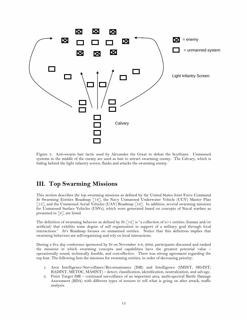
1. Scythians vs. Macedonians, Central Asian Operations of Alexander the Great, 329-327 B.C.. Scythians effectively used swarming horse-archers (“Parthian tactics”) to fight Alexander. Even though the horse-archers had great mobility and long-range arrow fire, Alexander eventually won using the anti-swarm “bait” tactic shown in Figure 3.

2. Parthian horse archers defeated the Romans in the Battle of Carrhae, 53 B.C.. Roman Legionaries carried a gladius (a short sword) and javelin, which was no match for the mounted archers who swarmed around the Romans and killed them with their bow and arrows.

3. At the Battle of Dorylaeum in 1097, the swarming Turkish horse archers initially surrounded the Crusaders and were on the verge of winning when another Crusader detachment arrived and surrounded the Turks, causing the battle to turn into a melee. The Crusaders won.

4. Mongol horse archers in the Battle of Liegnitz in 1241 were the ultimate swarmers. If they could not encircle the enemy, they used a feigned withdrawal. Mongol Toumens defeated their enemies using superior mobility and battlefield intelligence. Communication between groups included horns and flaming arrows. Mongol spies were always sent ahead as merchants.

More recent swarming cases include:

1. The woodland Indians surrounded and defeated a U.S. Army camp at St. Clair’s Defeat in 1791. 2. Napoleon’s operational swarming of the French during the Ulm Campaign in 1805. Napoleon

used four or five corps arranged in diamond formations. Each corp would fight and pin an entire opposing army for at least 24 hours, just enough time for sister corps to converge.

3. The German’s use of U-boat “Wolfpack” tactics during the Battle of the Atlantic is a naval example of swarming. Between 1939 and 1945, packs of five or more U-boats would converge on a convoy of transport ships and their destroyer escorts at night, independently attacking from multiple directions. The first boat to sight the convoy would begin shadowing it over the edge of the horizon by day, closing at dusk.

4. In 1993, Somalians swarmed towards the two U.S. helicopter crashes and the sound of firefights. Somalians converged on every street corner, shooting at the U.S. Commandos that were trying to escape. Somali civilians acted as sensors, pointing out the position of the U.S. Commandos. The Somalians had better situational awareness.

According to Edwards [2], the advantages of swarming are as follows.

1. It provides the unnerving psychological effect of being surrounded. 2. Dispersion of swarming units reduces vulnerability to WMD (Weapons of Mass Destruction).

r

4. ive at peace operations since while soldiers are dispersed around the world

shoul

er). In o r ust be good at these three factors. In the author’s

ll be re-entering this era of

3. It is good for COunterINsurgency (COIN) missions. COIN missions include physical “covedown” over a geographical area and pick up battlefield intelligence missed by airborne and spaceborne sensors. It maybe more effectthey may be performing peace-keeping activities.

d be noted that throughout history not all swarming tactics resulted in wins. After studying Ithistorical battles, Edwards suggests that three factors for successful swarming are

1. Elusiveness (mobility or concealment). 2. Superior situational awareness.

e firepow2. Standoff capability (longer rangrde to successfully swarm, unmanned systems m

opinion, one of the most difficult factors to satisfy will be concealment and “superior situational awareness.” As noted in an Army Science Board Study [13], perception of the environment is still the long pole in the tent for all unmanned systems; therefore, until the perception problem is solved, it will be difficult to achieve superior situational awareness on an autonomous platform.

rquilla [1] and Edwards [2] both suggest that the United States military wiAswarming as exemplified by the recent trend towards Network-Centric distributed small-unit forces. Even a recent article from MSNBC News illustrates the recent infatuation with swarming behaviors:

U.S. military aims to paralyze enemy Using 'swarm tactics,' Pentagon hopes for swift victorySWARM TACTICS

11

Of the 250,000 U.S. troops arrayed against Iraq, about 130,000 are in Kuwait. That would be the

91 war over the same ground, using so-called do

SNBC News, March 17, 2003

Note that the word “simultaneous” is crucial for military operations. Arquilla [1] also mentions that

note, it is also important to understand anti-swarming tactics. If swarming is to be the future of

main launching pad for a ground invasion, to include about 30,000 British troops. Franks is to command U.S. forced from his base in Qatar. The overall scenario would differ from the 19"swarm tactics" - simultaneous, coordinated attacks by air, conventional forces and commanunits, designed to confuse and overrun Iraqi defenders - would replace that war's five-week softening-up by airstrikes. M

communication was key to many advances in combat tactics. For example, early swarming attacks were signaled with flags, flaming arrows, or horns. As a final military operations, then the enemy may also use the same tactic. In fact, the anti-swarm tactics that Alexander used over 23 centuries ago are similar to modern U.S. counterinsurgency doctrine. U.S. Army Field Manual (FM) 90-8, Counterguerrila Operations, instructs soldiers to “locate, fix and engage.” Manuals FMs 7-10, 7-20, and 7-30 order soldiers to “find, fix, and finish” the guerrilla. The two techniques to engage elusive foes are either to block positions along likely escape routes or to encircle and cut off all ground escape routes and slowly contract the circle. One or more units in an encirclement can remain stationary while others drive the guerrilla force against them.

12

= enemy

= unmanned system

Light Infantry Screen

Calvary

Figure 3. Anti-swarm bait tactic used by Alexander the Great to defeat the Scythians. Unmanned systems in the middle of the enemy are used as bait to attract swarming enemy. The Calvary, which is hiding behind the light infantry screen, flanks and attacks the swarming enemy.

III. Top Swarming Missions This section describes the top swarming missions as defined by the United States Joint Force Command J9 Swarming Entities Roadmap [14], the Navy Unmanned Underwater Vehicle (UUV) Master Plan [15], and the Unmanned Aerial Vehicles (UAV) Roadmap [16]. In addition, several swarming missions for Unmanned Surface Vehicles (USVs), which were generated based on concepts of Naval warfare as presented in [8], are listed. The definition of swarming behavior as defined by J9 [14] is “a collection of n>1 entities (human and/or artificial) that exhibits some degree of self organization in support of a military goal through local interactions.” J9’s Roadmap focuses on unmanned entities. Notice that this definition implies that swarming behaviors are self-organizing and rely on local interactions. During a five day conference sponsored by J9 on November 4-8, 2002, participants discussed and ranked the missions in which swarming concepts and capabilities have the greatest potential value – operationally sound, technically feasible, and cost-effective. There was strong agreement regarding the top four. The following lists the missions for swarming entities, in order of decreasing priority:

1. Area Intelligence/Surveillance/Reconnaissance (ISR) and Intelligence (IMINT, SIGINT, RADINT, METOC, MASINT) – detect, classification, identification, neutralization, and salvage.

2. Point Target ISR – continued surveillance of an important area, multi-spectral Battle Damage Assessment (BDA) with different types of sensors to tell what is going on after attack; traffic analysis.

13

3. Communications / Navigation / Mapping – update of IPB; swarming supplementation of communication networks; and precision mapping of an area (surface or sub-surface).

4. Swarming Attacks 5. Defense / Protection – submarine warfare includes tagging by swarms, potential counter to

swarming boats; defensive operations for surface forces (flank protection). 6. Delay / Fix / Block 7. Deception Operations – UGV attack to emulate an attack pattern to cover an attack at another

point, decoys with swarm, jamming over whelm receivers for areas. 8. Search and Rescue (SAR) and Combat Search and Rescue – Applying swarms of UxVs to find

and/or retrieve personnel or other assets.

In addition to these missions, other possible unique or special applications of swarming entities were listed but not considered as primary missions. These include:

1. Clandestine or lethal obstacle clearance (minefields, toxic agents, bio hazards). 2. Recovery of objects, elements, or samples (e.g. ore, soil samples) in special environments. 3. Tracking and/or tagging operations (long-term surveillance) over wide areas or with many

targets (i.e., all the containers within a given port or ports within a region; ore shipments). 4. Airfield denial or aerial exclusion zones. 5. Urban operations: communications relays, surveillance, reconnaissance, tagging, and mapping. 6. Distributed, robust (graceful degradation) "phased-array" or multi-aspect sensors and/or

communications. 7. Subterranean operations / contained water body operations / subterranean "fluid” operations. 8. Logistics (user defined quantity, on demand, point or "home" delivery). 9. Undersea search and survey – mine counter measures, object sensing, and oceanography. 10. Navigation/Communication – On demand, subsurface data exchange between swarming entities. 11. Submarine track and trail – detect, classify, track, detect, support training, anti-submarine

warfare. 12. Recon – detect, classification, identification, neutralization, and salvage.

The UUV Master Plan [15] also defines four high priority missions:

1. Maritime reconnaissance – ISR, extending the reach into denied areas, and enabling missions in the littorals.

2. Undersea search and survey – mine counter measures, object sensing, and oceanography. 3. Communication/Navigation Aids – clandestine communication and navigation relay function,

data retrieval and exchange with subsea systems (buoys, arrays, etc.) 4. Submarine track and trail – detect, classify, track, detect, support training, anti-submarine

warfare. Several interesting perspective on Naval warfare are given in Hughes [17]. Weapon range and lethality have increased the size of the no man’s land between the fleets. Scouts and screens occupy the intervening space. Based on this fact, it appears that the first use of unmanned naval systems should be as scouts and screens. There is also a trend towards spreading forces out while using command and control to concentrate firepower from dispersed formations. The advantages of dispersion are 1) reduced signature and probability of detection by enemy, 2) reduced chances of mass destruction by WMD, and 3) break up of enemy assets. On the other hand, the advantages of massing are 1) collaborative support, and 2) increased striking power. Based on Hughes [17], the following missions are suggested as swarming Naval USV missions:

1. Maritime reconnaissance – ISR in no man zone between fleets, extending the reach into denied areas, and enabling missions in the littorals.

2. Maritime search and rescue 3. Communication/Navigation Aids – clandestine communication and navigation relay function. 4. In-port security and perimeter defense – e.g. USS Cole 5. Fleet escort

The UAV Roadmap [16] lists many missions for unmanned air vehicles (see Tables 1 and 2); however, it does not describe many missions that require large swarming numbers. Shaw [18] explains that manned

14

aircraft rarely fly combat missions in numbers greater than 2 or 4. Two fighter aircraft (called a Section) is considered by most military doctrines to be the ideal mutual supporting element. Manned aircraft rarely fly in groups greater than 4 (a Division consists of 2 Sections). Problems with larger numbers includes:

• Increased probability of detection (wider RADAR cross-section). Surprise is nine-tenths of air combat success.

• Divided attention of pilot to keep track of wingman. • Formation tactics usually result in reduced aircraft performance. • Increased communication (problems with attendant task loading and greater probability of

electronic detection). For these reasons, swarming UAVs have not been viewed as a high priority.

Table 1. CINC/Service UAV Mission Prioritization Matrix – 2000. Predator Global

Hawk TUAV VTUAV IPLs

Reconnaissance 1 1 1 1 1 Signals Intelligence 3 2 7 4 4 Mine Countermeasures 7 12 4 5 10 Target Designation 2 11 3 2 - Battle Management 8 7 5 7 - Chem-Bio Recon 10 10 6 9 5 Counter CC&D 4 5 8 11 - Electronic Warfare 6 4 9 10 7 Combat SAR 5 8 10 8 8 Comm/Data Relay 9 3 2 3 2 Information Warfare 11 6 11 6 - Digital Mapping 12 9 12 12 - * IPL = Integrated Priority List

Table 2. SOCOM UAV Mission Prioritization Matrix – 2000. Predator Global

Hawk TUAV VTUAV

Reconnaissance - 5 7,8 7,8 Signals Intelligence - 7 15 11 Mine Countermeasures 10 12 11 11 Target Designation 6 6 6,14 6,14 Battle Management 7 8 16 16 Chem-Bio Recon 1 1 1 1 Counter CC&D - 10 18 18 Electronic Warfare - - 19 19 Combat SAR - 11 17 17 Comm/Data Relay 4,11 3 4,13 4,13 Information Warfare 8 9 5 5 Digital Mapping 5 4 - - PSYOP (broadcast/leaflets) 2 2 2 2 Covert Sensor Emplacement 2 - 3 3 Decoy/Pathfinder - - 9 9 Team Resupply 9 - 10 10 Battle Damage Assessment 12 - 12 12 GPS Pseudolite - 13 - - Weather - 14 - -

However, one application where multiple UAVs does make sense is DARPA’s Net Fires program. In this program, multiple Precision Attach Missiles (PAMs) and Loitering Attack Missiles (LAMs) may be used

15

to attack multiple moving ground targets. As part of this project, Sandia has looked at the cooperative behaviors required for this mission. A separate report was written to discuss the cooperative behaviors used to control these missiles [19].

IV. Generic Behaviors As shown in the previous section, there are many possible military missions for cooperative unmanned systems. In this section, we will only consider the top 8 missions as identified by the U.S. Joint Force Command. Given these missions, the next questions to ask are:

• Are there generic behaviors that can be reused regardless of whether the mission is on land, sea, or air?

• Can we categorize these behaviors?

According to Edwards [2], the four stages of swarming are locate, converge, attack, and disperse. These stages occur in succession during the evolving conflict. It should be noted that these same stages have been identified by other researchers when describing the swarming of insects [20]. While these four stages are certainly evident in a conflict, we suggest that additional stages are required to perform the top 8 missions. We suggest that these missions could be accomplished with 9 generic swarming behaviors as shown in the columns in Table 3. The categorization of these behaviors is based on algorithms that the authors have developed and algorithms that have been found in the literature. This categorization is not unique, and as additional algorithms are developed, these algorithms may fall into one of these categories or new behavior categories may need to be formed.

Table 3. Reusable generic behaviors that can be applied to top 8 swarming missions. An ‘x’ indicates that the cooperative behavior may be used in a mission. A ‘c’ stands for combat.

Missions/Coop. Behaviors

For

mat

ion

Map

ping

/Sur

vey C

over

age

Con

tain

men

t

Con

verg

ing

Sear

ch

Det

ect/

Tra

ck

Pur

suit

Eva

sion

Area ISR x x x Point ISR x x x x Comm/Navigation/Mapping x x x x Swarming Attacks x x x x x x x x x Defense/Protection x x x Delay/Fix/Block x x x Deception Operations x x x (Combat) Search and Rescue x x x c

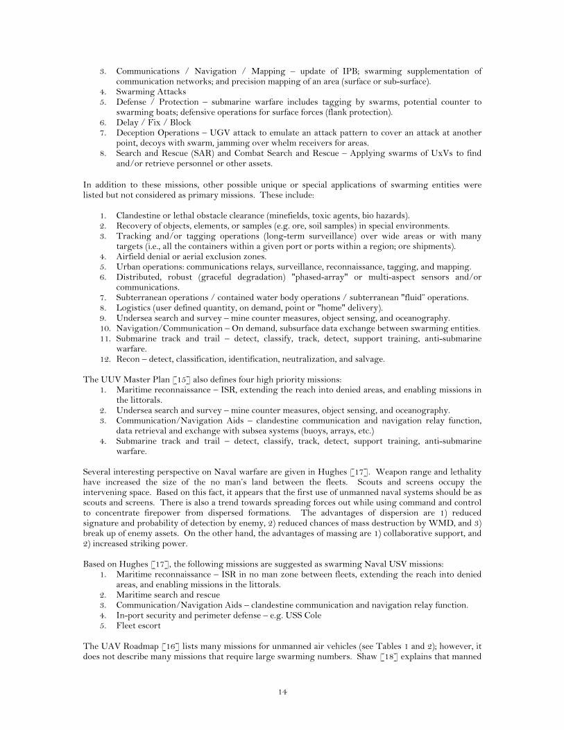
* Localization is not listed as a behavior because it is an essential part of all behaviors. These behaviors are typically instantiated sequentially over the mission. For example in a swarming attacks mission as shown in Figure 4, the group of unmanned vehicles might perform the following tasks. First, the group of unmanned vehicles might first drive in formation to the planned location of an ambush. Formation behaviors allow a single operator to guide multiple entities to a desired end point while staying in a specified geometric formation. Over the past several years, many researchers have developed formation behaviors [21-25].

Drive in Formation to Location X

16

Map area A around Location X Search Area B around Location X and/or

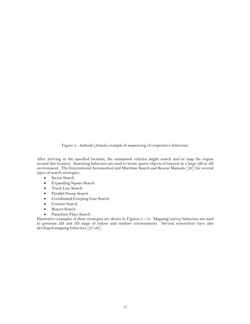
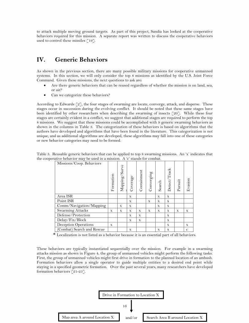
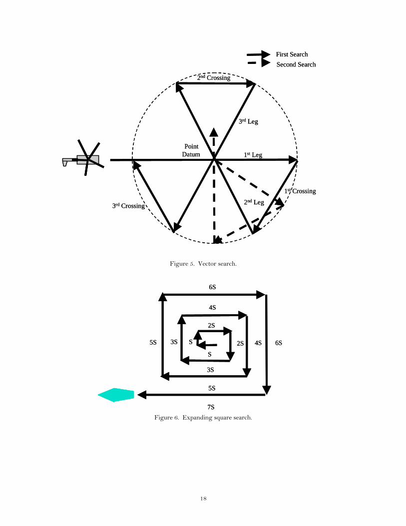
Figure 4. Ambush (Attack) example of sequencing of cooperative behaviors. After arriving at the specified location, the unmanned vehicles might search and/or map the region around this location. Searching behaviors are used to locate sparse objects of interest in a large 2D or 3D environment. The International Aeronautical and Maritime Search and Rescue Manuals [26] list several types of search strategies:

• Sector Search • Expanding Square Search • Track Line Search • Parallel Sweep Search • Coordinated Creeping Line Search • Contour Search • Beacon Search • Parachute Flare Search

Illustrative examples of these strategies are shown in Figures 5 - 13. Mapping/survey behaviors are used to generate 2D and 3D maps of indoor and outdoor environments. Several researchers have also developed mapping behaviors [27-29].

17

1st Leg

2nd Leg

1st Crossing

2nd Crossing

3rd Leg

3rd Crossing

First Search

Second Search

Point Datum 1st Leg

2nd Leg

1st Crossing

2nd Crossing

3rd Leg

3rd Crossing

First Search

Second Search

Point Datum

Figure 5. Vector search.

S

S

2S

2S

3S

3S

4S

4S

5S

5S

6S

6S

7S

S

S

2S

2S

3S

3S

4S

4S

5S

5S

6S

6S

7S

Figure 6. Expanding square search.

18

0.5STrack of Missing Aircraft

0.5S

Track Search Return (TSR)

STrack of Missing Aircraft

S

Track Search Non-return (TSN)


0.5S



0.5S



S



S


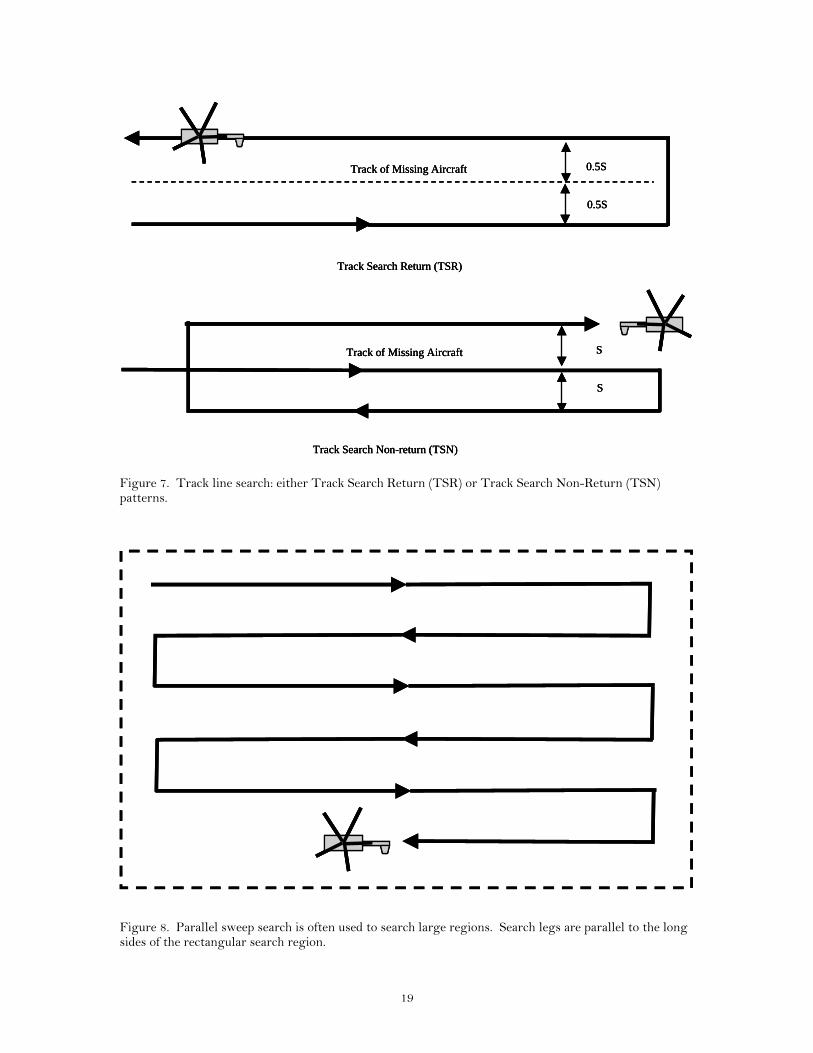
Figure 7. Track line search: either Track Search Return (TSR) or Track Search Non-Return (TSN) patterns.

Figure 8. Parallel sweep search is often used to search large regions. Search legs are parallel to the long sides of the rectangular search region.

19

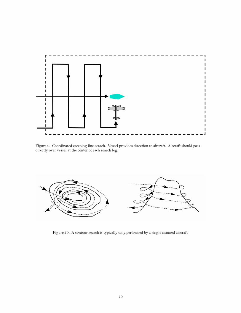
Figure 9. Coordinated creeping line search. Vessel provides direction to aircraft. Aircraft should pass directly over vessel at the center of each search leg.

Figure 10. A contour search is typically only performed by a single manned aircraft.

20

Max Range of Signal

Location of ELT

Descending

Signal Fades

Signal Heard

Signal Fades

Signal Heard

Max Range of Signal

Location of ELT

Descending

Signal Fades

Signal Heard

Signal Fades

Signal Heard

Figure 11. Map-assisted aural electronic beacon search.

Location of ELT

Signal HeardStart Timing

Signal FadesCheck TimeTurn 180

Signal FadesCheck TimeTurn 180 Signal Heard

Start Timing

½ TimeTurn 90


½ Time

Location of ELT

Signal HeardStart Timing


Signal FadesCheck TimeTurn 180 Signal Heard

Start Timing

½ TimeTurn 90


½ Time

21

Figure 12. Time-assisted aural electronic beacon search.

Figure 13. Parachute flare search.

ext, the group of unmanned vehicles might cover or contain the region. The word coverage refers to

nce dispersed, the unmanned vehicles might detect and track intruders as they enter the region. This

inally, the unmanned vehicles might converge, pursue, or evade from the intruders depending whether

Ship’s Relative Wind

Ship’s Track

Burn-out Burn-out

Flare Flare

Ship’s Relative Wind

Ship’s Track

Burn-out Burn-out

Flare Flare

Ndispersing the unmanned vehicles throughout the entire region. For UGVs, this means to disperse in two dimensions. For UUVs and UAVs, this means to disperse in three dimensions. The word containment implies to disperse the unmanned vehicles over a subspace of dimension at least one less than the space of interest. For UGVs, this means to disperse along a one-dimensional curve around the two dimensional area. For UUVs and UAVs, this means to disperse along the two-dimensional surface surrounding the three-dimensional volume. Ocooperative behavior requires that multiple unmanned vehicles share information on their observations to obtain a better estimate of the intruder’s position. Distributed Kalman or information filters are often used to provide optimal estimates [30]. Fthe group is winning or losing the current battle. Convergent behaviors cause multiple unmanned vehicles to simultaneously gather together or converge around the target of interest. In contrast, multiple vehicles will not simultaneously converge on the target in a cooperative pursuit. Instead, one vehicle might chase the target while other vehicles might “head the target off at the pass.” Often game theory techniques are used to develop cooperative pursuit behaviors that maximize the probability of capture or kill [31]. Evasion behaviors are used to escape from the enemy. The goal of this behavior is to maximize the probability of escape. Examples of evasive behaviors include 1) dispersing unpredictably in all directions, and 2) acting as sacrificial decoys so as to increase chances that a select few (possibly manned) escape. This behavior may be one of the easiest collective behaviors in that dispersing unpredictably is relatively easy to do.

22

V. Common Mathematical Framework

this section, a common mathematical framework that can be used to describe a number of cooperative

his mathematic framework is motivated by the fact that most of the laws in physics and mechanics can

Table 4. Lagrangian for various physical phenomena [32].

Phenomenon Lagrangian

Inbehaviors is developed. This mathematical framework is applied to three of the generic behaviors listed in the previous section: containment, coverage, and converging. The authors believe that this same framework could be applied to the other behaviors, although this has not been proven at the time of this publication. Tbe derived by finding the maximum or minimum of some performance index, in this case, called the Lagrangian integral. In Table 4, notice that the Lagrangian of each phenomenon is a function of some gradient term squared. In the analysis that follows, you will notice that each behavior’s performance index is also a function of some gradient term squared.

Classical Mechanics

Vtq ⎞⎛ ∂1

m −⎟⎠

⎜⎝ ∂

2

2

Flexible String or Compressible Fluid

Diffusion Equation

⎥⎥⎦

⎤

⎢⎢⎣

⎡∇•∇−⎟

⎠⎞

⎜⎝⎛∂∂

qqct

q 22

2

1 ρ

K−∇•∇− *ψψ

Schrodinger Equation

Electromagnetic Equations

Kh

−∇•∇− *

2ψψ

m

K−∇•∇∑=

nnn

qq4

14

Boltmann Law

K−⎟⎠⎞

⎜⎝⎛∂∂ 2

4Eq

ollowing this same optimization approach, a three-step process for developing cooperative control gorithms has been developed [48]. These three steps are as follows:

l entities. . Partition and eliminate terms in the performance index so that only terms of local neighbors are

performance index.

understands the problem well enough that it can be posed as a global ptimization problem. This step can be relatively difficult, but as the examples in the remainder of this

Fal 1. Define a global performance index as a function of parameters from al2included. 3. The local control law is the gradient (or the product of the inverse Hessian and gradient) of the partitioned The first step requires that oneosection will show, that with the right simplifying assumptions, rather simple equations can be used to solve difficult problems.

23

The second step, partitioning the performance index, is often used in parallel optimization to reduce the omputation time for large-scale problems [33]. In this case, the second step is used to reduce

dex using either a first-order eepest descent algorithm or second order method such as the Newton’s Method [34].

in practice. Six xamples are given with details on the problem formulation and the task that was performed.

.1. Example 1: Spreading Apart along a Line – A Containment Behavior

ly spread part along a straight line using only information from the neighboring robots on the right and left. In

ccommunications between robots and to increase robustness of the distributed system. The control law that would result from step 1 would require that every robot be able to communicate with all the other robots. As the number of robots increase to 100s and 1000s, the time delay necessary for communication would make the resulting control infeasible. Instead, partitioning the performance index and eliminating terms to include only terms of local neighbors results in a control law that only requires communication with nearest neighbors, thus greatly reducing communication delay. Also, using nearest neighbors that change throughout the motion adds an element of robustness. The mathematical formulation of the partition does not specify that robot number 10 must communicate with robot number 6. Instead, the mathematical formulation specifies a group of nearest neighbors that can change based on external forces and environmental conditions. This creates an element of self-organization that allows the system to change and evolve. If a robot fails, a new set of nearest neighbors is formed. The third step is to solve for the extremum of the partitioned performance inst The remainder of this section will be spent showing how these three steps have been usede V This first example is a simple one-dimensional problem. The goal is for multiple robots to evenaFigure 14, the first and last robots are assumed to be stationary while the ones in between are to spread apart a distance d away from each other.

2

3

4

t= 0

x

1

t= tf

x

1 2 3 4

Figure 14. One-dimensional control problem. The top line is the initial state. The second line is the desired final state. Vehicles 1 and 4 are boundary conditions. Vehicles 2 and 3 spread out along the line

he optimization steps are as follows.

lem, the objective is to

using only the position of their left and right neighbors. T Step 1. Specified as an optimization prob

)(min xvx

(1)

where the global performance index is

24

21

112

1)( ∑ ⎟

⎠⎞⎜

⎝⎛ −−=

−

=+

n

iii xxdxv , (2)

is the position of robot i, ix [ ]Tnxxx ...1= are the positions of all the robots, and d is the desired dis The goal is to m

tep 2. This problem is easily partitioned amongst the interior n-2 robots. The distributed objective is to

tance between each robot. inimize the sum of squared errors in distances between every robot. S

1,...2)(min −=∀ nixvi (3) xi

where the partitioned performance index is 2

1

2

1 2

1

2

1 ⎛)( ⎟⎠⎞⎜

⎝⎛ −−+⎟

⎠⎞⎜

⎝−−= +− iiiii xxdxxdxv . (4)

Because of the additive form of Equation (2), simultaneously solving Equation (3) for eac

tep 3. A steepest descent control law for the partitioned performance index is given by

h robot is the same as minimizing the global performance index in Equation (2). Therefore, in this case, no terms were eliminated. This is not necessarily true for the other example problems below. S

( ) ( ) ( ) 10,)(1 ≤<∇−=+ αα kxvkxkx ii , i (5) where

( ) 1111 if2)( +−−+ <<+−=∇ iiiiiii xxxxxxxv . (6)

when ( )112

1−+ += iii xxx0)( =∇ xviNote that . Therefore, the vehicles will disperse along the line until

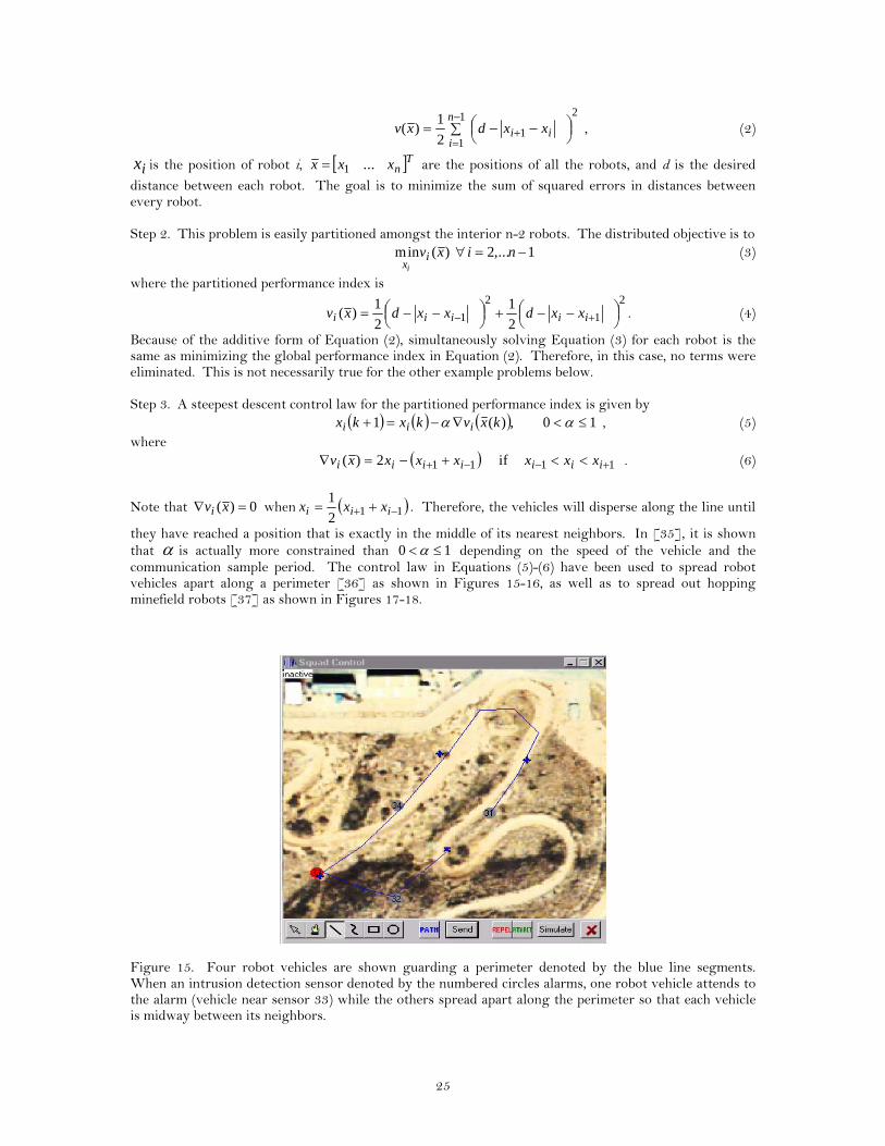
exactly in the mithey have reached a position that is ddle of its nearest neighbors. In [35], it is shown that α is actually more constrained than 10 ≤<α depending on the speed of the vehicle and the communication sample period. The control Equations (5)-(6) have been used to spread robot vehicles apart along a perimeter [36] as shown in Figures 15-16, as well as to spread out hopping minefield robots [37] as shown in Figures 17-18.

law in

igure 15. Four robot vehicles are shown guarding a perimeter denoted by the blue line segments. FWhen an intrusion detection sensor denoted by the numbered circles alarms, one robot vehicle attends to the alarm (vehicle near sensor 33) while the others spread apart along the perimeter so that each vehicle is midway between its neighbors.

25

Figure 16. Robot vehicles used to perform perimeter surveillance task.

Breach

Hopping landmine robots

Enemy Breach Vehicle

igure 17. Hopping landmine robots are filling breach left by enemy vehicle. When a robot is reached, F b

the robots will hop towards the missing robot and settle when each robot is midway between its neighbors.

26

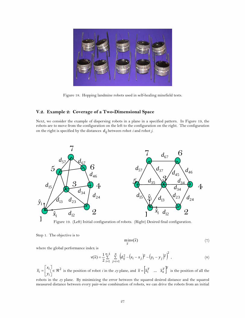
Figure 18. Hopping landmine robots used in self-healing minefield tests.

V.2. Example 2: Coverage of a Two-Dimensional Space Next, we consider the example of dispersing robots in a plane in a specified pattern. In Figure 19, the robots are to move from the configuration on the left to the configuration on the right. The configuration on the right is specified by the distances between robot i and robot j. ijd

Figure 19. (Left) Initial configuration of robots. (Right) Desired final configuration.

5

1

3 24d

12d

13d

1̂x

1̂y

2

4

23d34d

15d

57d6

7 67d

46d5

1

3

24d

12d

13d

1̂x

1̂y

2

4 34d

15d

45d

35d

57d

7 6 67d

37d46d

34d

23d

Step 1. The objective is to

)(min xvx

(7)


( ) ( )( )21

1 1

222

2

1)( ∑ ∑ −−−−=

−

= +=

n

i

n

ijjijiij yyxxdxv , (8)

2ℜ∈⎥⎦

⎤⎢⎣

⎡=

i

ii y

xx is the position of robot i in the xy plane, and [ ]TT

nT xxx ...1= is the position of all the

robots in the xy plane. By minimizing the error between the squared desired distance and the squared measured distance between every pair-wise combination of robots, we can drive the robots from an initial

27

pattern to the desired specified pattern. Notice that the global performance index does not specify the orientation or final absolute position of the group of robots. Step 2. The global performance index is over constrained since it is possible to achieve the same minimum solution without having to minimize the error between every pair-wise combination. The same minimum solution can be achieved by only minimizing the error between neighboring robots. The distributed objective is to

nixvixi

,...,1)(min =∀ (9)

where the partitioned performance index is

( ) ( )( 2222

21

)( ∑ −−−−=∈NNj

jijiiji yyxxdxv ) (10)

and NN stands for nearest neighbor. Step 3. The steepest descent control law for the partitioned performance index is given by

( ) ( ) ( ) 10,)(1 ≤<∇−=+ αα kxvkxkx iii (11) where

2ℜ∈

⎥⎥⎥⎥

⎦

⎤

⎢⎢⎢⎢

⎣

⎡

∂∂∂∂

=∇

i

i

i

i

i

y

vx

v

v , (12)

( ) ( )[ ]( jiNNj

jijiiji

i xxyyxxdx

xv−∑ −−−−−=

∂∂

∈

2222)( ) , (13)

( ) ( )[ ] ( jiNNj

jijiiji

i yyyyxxdy

xv−∑ −−−−−=

∂∂

∈

2222)( ) . (14)

Note that when 0=∇ iv ( ) ( ) NNjyyxxd jijiij ∈−+−= for222 . In [38], the connective stability of

this control law is proven using a vector Liapunov technique. The control law in Equations (11)-(14) has been used to spread apart the hopping minefield robots as shown in Figure 20. In this case, the specified

distances are all equal and the number of nearest neighbors used for control is three. ijd

28

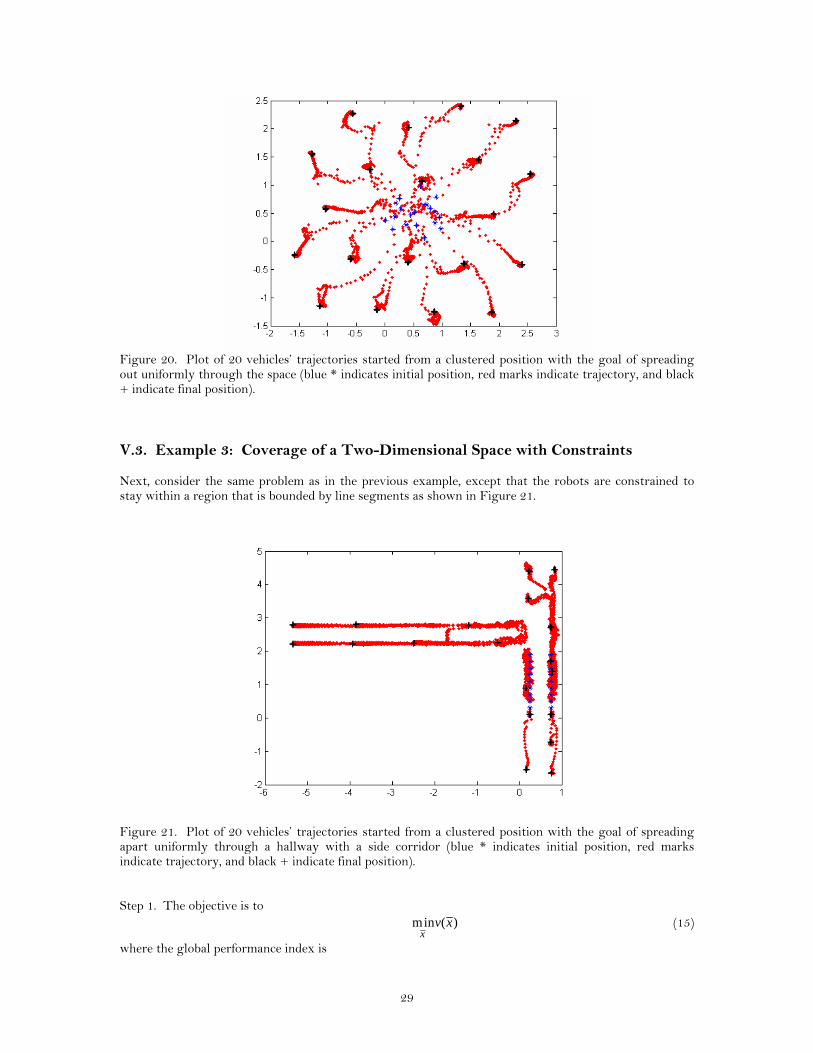
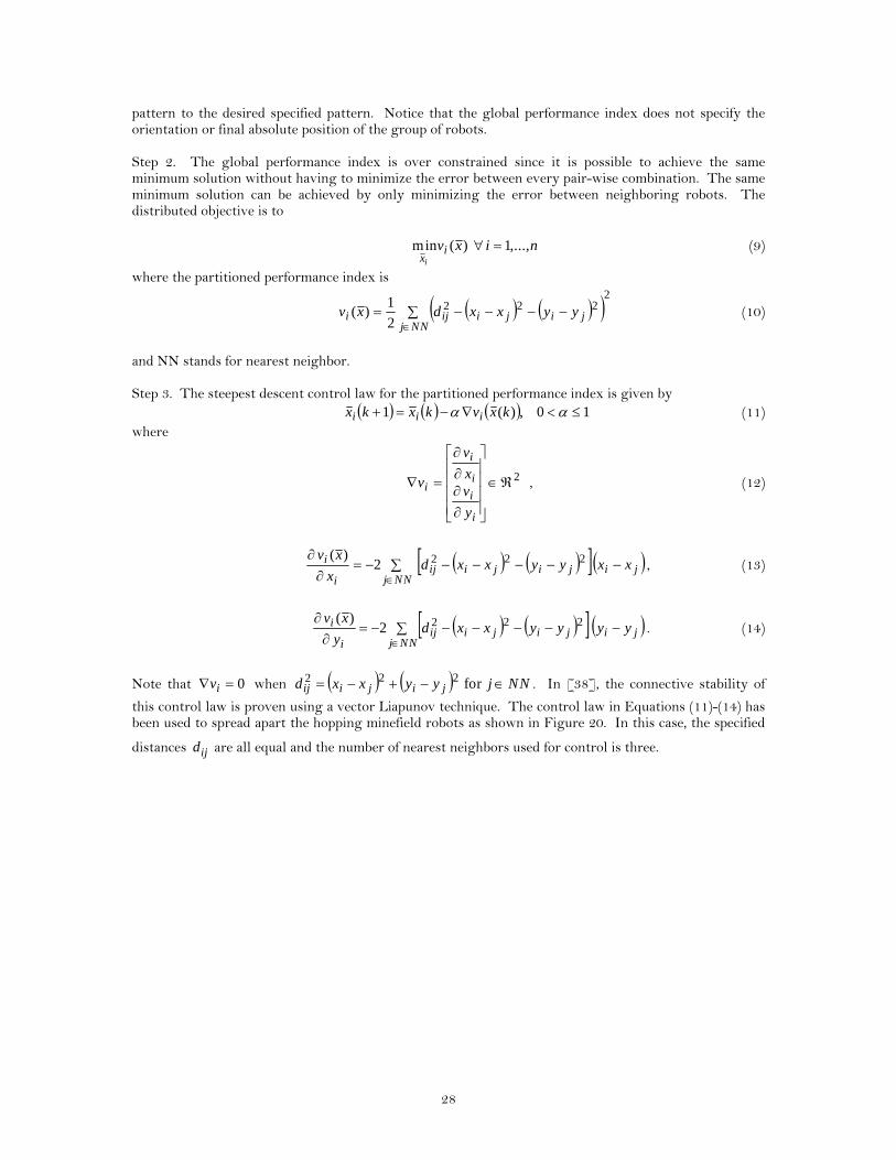
Figure 20. Plot of 20 vehicles’ trajectories started from a clustered position with the goal of spreading out uniformly through the space (blue * indicates initial position, red marks indicate trajectory, and black + indicate final position). V.3. Example 3: Coverage of a Two-Dimensional Space with Constraints Next, consider the same problem as in the previous example, except that the robots are constrained to stay within a region that is bounded by line segments as shown in Figure 21.

Figure 21. Plot of 20 vehicles’ trajectories started from a clustered position with the goal of spreading apart uniformly through a hallway with a side corridor (blue * indicates initial position, red marks indicate trajectory, and black + indicate final position). Step 1. The objective is to

)(min xvx

(15)


29

21

1 1

22

2

1)( ∑ ∑ ⎟

⎠⎞

⎜⎝⎛ −−=

−

= +=

n

i

n

ijjiij xxdxv (16)

subject to nibxA i ,...,1=∀≤ (17)

where and . Equation (17) specifies the boundary conditions of m straight-line segments.

2×ℜ∈ mA mb ℜ∈

Step 2. The distributed objective is to

ixvixi

∀)(min (17)


( 22

22

2

1

2

1)( −

∈∈−∑Λ+∑ ⎟

⎠⎞

⎜⎝⎛ −−= lil

NOlNNjjii bxAxxdxv ) . (18)

Here, the inequality constraints in Equation (17) have been added as a weighted penalty function that is the sum of the inverse squared perpendicular distances between robot i and the nearest obstacle (NO) line segments l. The is a scalar used to vary the importance of obstacle avoidance. As before, NN stands for the set of nearest neighbors. Similarly, the set NO is the set of nearest obstacles.

Λ

Step 3. The steepest descent control law is

( ) ( ) ( ) 10,)(1 ≤<∇−=+ αα kxvkxkx iii (19) where

( ) ( 3222)( −

∈∈−∑Λ−−⎟

⎠⎞

⎜⎝⎛ −−∑−=∇ lil

Tl

NOljiji

NNii bxAAxxxxdxv ) (20)

The control law in Equations (19) and (20) has been used to spread out the robot vehicles in a hallway as shown in Figure 21. The nearest obstacles are determined from IR proximity sensors. The specified distance d between vehicles was chosen to be within the 10 meter acoustic range of the sensors on top of the vehicle (see Figure 22) [39]. Again, the number of nearest neighbors used for control is three.

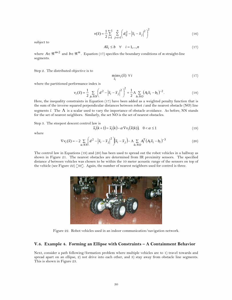
Figure 22. Robot vehicles used in an indoor communication/navigation network. V.4. Example 4. Forming an Ellipse with Constraints – A Containment Behavior Next, consider a path following/formation problem where multiple vehicles are to 1) travel towards and spread apart on an ellipse, 2) not drive into each other, and 3) stay away from obstacle line segments. This is shown in Figure 23.

30

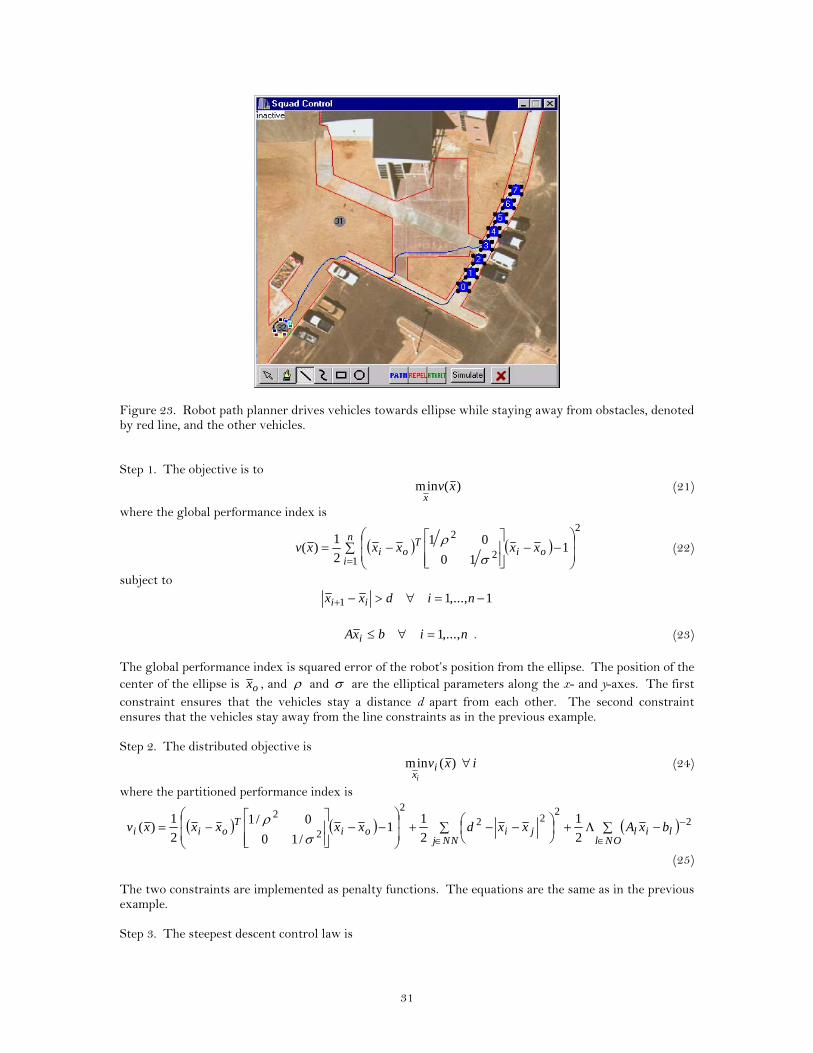
Figure 23. Robot path planner drives vehicles towards ellipse while staying away from obstacles, denoted by red line, and the other vehicles. Step 1. The objective is to

)(min xvx

(21)


( ) ( )2

12

21

10

012

1)( ∑ ⎟

⎟

⎠

⎞

⎜⎜

⎝

⎛−−

⎥⎥⎦

⎤

⎢⎢⎣

⎡−=

=

n

ioi

Toi xxxxxv

σρ (22)

subject to 1,...,11 −=∀>−+ nidxx ii

nibxA i ,...,1=∀≤ . (23)

The global performance index is squared error of the robot’s position from the ellipse. The position of the center of the ellipse is ox , and ρ and σ are the elliptical parameters along the x- and y-axes. The first constraint ensures that the vehicles stay a distance d apart from each other. The second constraint ensures that the vehicles stay away from the line constraints as in the previous example. Step 2. The distributed objective is

ixvixi

∀)(min (24)


( ) ( ) ( 22

222

2

2

2

1

2

11

/10

0/12

1)( −

∈∈−∑Λ+∑ ⎟

⎠⎞

⎜⎝⎛ −−+

⎟⎟

⎠

⎞

⎜⎜

⎝

⎛−−

⎥⎥⎦

⎤

⎢⎢⎣

⎡−= lil

NOlNNjjioi

Toii bxAxxdxxxxxv

σρ )

(25) The two constraints are implemented as penalty functions. The equations are the same as in the previous example. Step 3. The steepest descent control law is

31

( ) ( ) ( ))(1 kxvkxkx iii ∇−=+ α (26) where

( ) ( ) ( )

( ) ( ) 322

2

2

2

2

2

/10

0/11

10

012)(

−

∈∈−∑Λ−−⎟

⎠⎞

⎜⎝⎛ −−∑−

−⎥⎥⎦

⎤

⎢⎢⎣

⎡⎟⎟

⎠

⎞

⎜⎜

⎝

⎛−−

⎥⎥⎦

⎤

⎢⎢⎣

⎡−=∇

lilTl

NOljiji

NNj

oioiT

oii

bxAAxxxxd

xxxxxxxvσ

ρσ

ρ

(27)

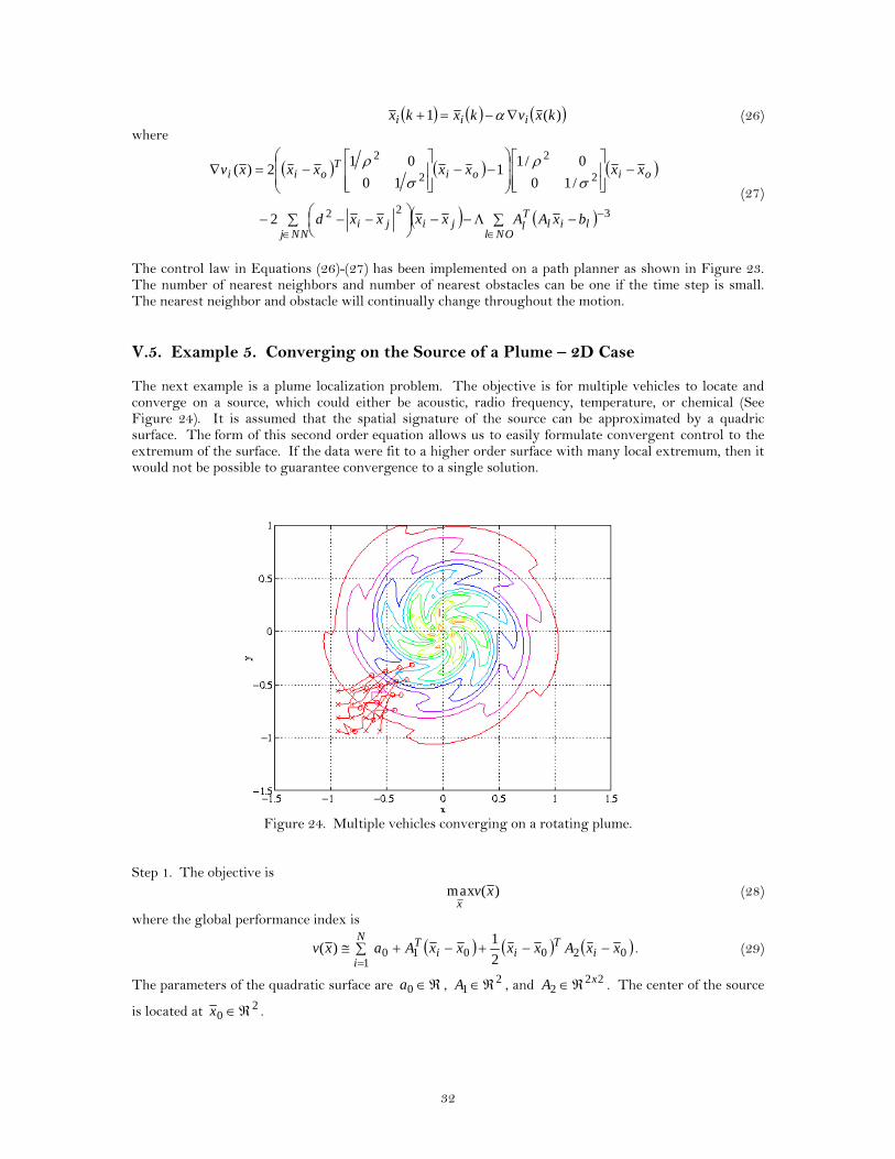
The control law in Equations (26)-(27) has been implemented on a path planner as shown in Figure 23. The number of nearest neighbors and number of nearest obstacles can be one if the time step is small. The nearest neighbor and obstacle will continually change throughout the motion. V.5. Example 5. Converging on the Source of a Plume – 2D Case The next example is a plume localization problem. The objective is for multiple vehicles to locate and converge on a source, which could either be acoustic, radio frequency, temperature, or chemical (See Figure 24). It is assumed that the spatial signature of the source can be approximated by a quadric surface. The form of this second order equation allows us to easily formulate convergent control to the extremum of the surface. If the data were fit to a higher order surface with many local extremum, then it would not be possible to guarantee convergence to a single solution.

Figure 24. Multiple vehicles converging on a rotating plume.

Step 1. The objective is

)(max xvx

(28)


( ) ( ) ( 0200101 2

1)( xxAxxxxAaxv i

Tii

TN

i−−+−+∑≅

=) . (29)

The parameters of the quadratic surface are ℜ∈0a , , and . The center of the source

is located at

21 ℜ∈A 22

2xA ℜ∈

20 ℜ∈x .

32

Step 2. The distributed objective is ixvi

xi

∀)(max (30)


( ) ( ) ( ijiT

ijijTii

NNji xxAxxxxAaxv −−+−+∑≅

∈210 2

1)( ) (31)

Each vehicle determines it’s own estimate of the quadratic surface using information from its nearest neighbors. An alternative approach is to use data from as many neighbors as possible and calculate a least-squares estimate of the quadratic coefficients. References [40-41] describe the least squares fitting algorithm in more detail. Step 3. The second order Newton’s method control law is

( ) ( ))(1

)(

121

kxikx

iii AAkxkx −−=+ α (32)

where the quadratic coefficients are determined from the solution to the nearest neighbor equations

( ) ( ) ( ) ( ) NNjxxAxxxxAaxv ijTi

Tijij

Tiiji ∈∀−−+−+= 210 2

1 (33)

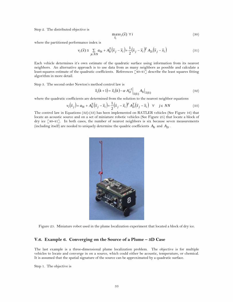
The control law in Equations (32)-(33) has been implemented on RATLER vehicles (See Figure 16) that locate an acoustic source and on a set of miniature robotic vehicles (See Figure 25) that locate a block of dry ice [40-41]. In both cases, the number of nearest neighbors is six because seven measurements (including itself) are needed to uniquely determine the quadric coefficients and . iA1 iA2

Figure 25. Miniature robot used in the plume localization experiment that located a block of dry ice. V.6. Example 6. Converging on the Source of a Plume – 3D Case The last example is a three-dimensional plume localization problem. The objective is for multiple vehicles to locate and converge in on a source, which could either be acoustic, temperature, or chemical. It is assumed that the spatial signature of the source can be approximated by a quadratic surface. Step 1. The objective is

33

)(max xvx

(34)


( ) ( ) ( 0200101 2

1)( xxAxxxxAaxv i

Tii

TN

i−−+−+∑≅

=) . (35)

The parameters of the quadratic surface are ℜ∈0a , , and . The center of the source

is located at

31 ℜ∈A 33

2xA ℜ∈

30 ℜ∈x .

Step 2. The distributed objective is

ixvixi

∀)(max (36)


( ) ( ) ( ijiT

ijijTii

NNji xxAxxxxAaxv −−+−+∑≅

∈210 2

1)( ) (37)

Each vehicle determines it’s own estimate of the quadratic surface using information from its nearest neighbors. Step 3. The second order Newton’s method control law is

( ) ( ))(1

)(

121

kxikx

iii AAkxkx −−=+ α (38)

where the quadratic coefficients are determined from the solution to the nearest neighbor equations

( ) ( ) ( ) ( ) NNjxxAxxxxAaxv ijTi

Tijij

Tiiji ∈∀−−+−+= 210 2

1 (39)

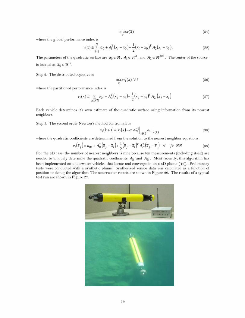
For the 3D case, the number of nearest neighbors is nine because ten measurements (including itself) are needed to uniquely determine the quadratic coefficients and . Most recently, this algorithm has been implemented on underwater vehicles that locate and converge in on a 3D plume [42]. Preliminary tests were conducted with a synthetic plume. Synthesized sensor data was calculated as a function of position to debug the algorithm. The underwater robots are shown in Figure 26. The results of a typical test run are shown in Figure 27.

iA1 iA2

34

Figure 26. Nekton Research underwater vehicle used to locate synthetic plume source.

Figure 27. Underwater synthetic plume test results. These six examples demonstrate the utility of this three-step process for creating locally optimal distributed controls for multiple robotic vehicles. The resulting control laws are robust and only require sharing of information between nearest neighbors. The robustness is the result of the self-organizing nature of the control where nearest neighbors are continually changing throughout the motions. If a vehicle is lost or dies, another set of nearest neighbors can be used to complete the task. By using penalty functions to approximate constraints, the control laws are in a form that is identical to the potential field control laws often used for controlling single and multiple robots. The main difference is the switching of potential fields based on the nearest neighbors and the nearest obstacles. VI. Behavior Metrics In this section, two metrics are developed for comparing similar cooperative behaviors. The first metric is the global performance index described in the previous section. The second metric is the time required to converge to the behavior’s final state. There are many other possible metrics that need to be investigated in the future. These include the algorithm’s robustness to failure, required on-board computing, and required sensing. There are also behavior-specific metrics that need further investigation. For example, the probability of detection and false alarm rates are important metrics that must be evaluated for a search behavior. In the cooperative Net Fires report [19], the system-level cumulative probability of detection was evaluated for different search patterns.

35

Based on the analysis in the previous section, the most obvious metric for measuring the performance of a cooperative behavior is the global performance index used to create the behavior. For example in the containment behavior for spreading out on a line, the global performance index defined in Equation (2) can be used to measure the effectiveness of the distributed control law. Because of the partitioning step used to determine local behaviors, the global performance index will often not be zero. This implies that the best distributed control behaviors will partition the problem and choose local neighbor interactions such that the global performance index is minimized. The global performance indices described in the previous section are not a function of time. Instead, they minimize the final goal position of the robots. Another metric that is much more difficult to evaluate is the time required to converge to the behavior’s final state. Because many of the interactions between vehicles depend on information that is shared over a radio, this metric depends heavily on the communication overhead and network configuration time. The communication bandwidth and latency will greatly affect the stability and performance of the system. Within this project, previous analysis regarding stable control of multiple vehicles using large-scale decentralized control techniques [35] has been extended to include the communications aspects of the problem. A stability analysis shows that the local feedback control gains of the robotic vehicles must be decreased if the communication sample period is increases. Therefore, there is a tight coupling between communications and controls that cannot be ignored. In general, a system will be more responsive and have shorter settling times if the feedback control gains are as large as possible and the communication sample period is as short as possible. This section evaluates the resulting communication sample period of four different communication protocols: a Time Division Multiple Access (TDMA) linear broadcast, a TDMA polylogarithmic broadcast, a TDMA coloring algorithm, and a Collision Sense Multiple Access (CSMA) coloring algorithm. The selection of the best protocol depends on the density of the robot vehicles and the communication radius of each vehicle. Throughout this section, the one-dimensional dispersion example from the previous section is used to illustrate the design methodology. In [35], it is shown that α in Equation (5) is actually more constrained than 10 ≤<α depending on the speed of the vehicle and the communication sample period. Therefore, the next question to ask is that of connective stability. Under what conditions will the overall system be globally asymptotically stable even under structural perturbations? Analysis of connective stability is based upon the concept of vector Liapunov functions, which associates several scalar functions with a dynamic system in such a way that each function guarantees stability in different portions of the state space. The objective is to prove that there exist Liapunov functions for each of the individual subsystems and then prove that the vector sum of these Liapunov functions is a Liapunov function for the entire system. To simplify matters, we will assume that the control function has already been chosen and the closed loop dynamics of the discrete time system can be written as

( ) ( ) { }.,...,1,,~),(1: Nixkgxkgkx iiii ∈+=+S (40)

where ( ) nkx ℜ∈ is the state of (e.g., x, y position, orientation, and linear and angular velocities of all

vehicles) at time , is the state of the i

S

Tk∈ ( ) ini kx ℜ∈ th subsystem at time . The function

describes the local dynamics of , and the function represents

the dynamic interaction of with the rest of the system . The interconnection function can be written as

iS Tk∈

ii nni Tg ℜ→ℜ×: iS inn

i Tg ℜ→ℜ×:~

iS S

( ) ( ) { }Nixexexekgxkg NiNiiii ,...,1,...,,,~,~2211 ∈= (41)

where ji nnij Be

×∈ , and the elements of the fundamental interconnection matrix ( )ijeE = are

( ) ( ) ( )( )( ) ( )(⎪⎩

⎪⎨⎧

=.,,~,0

,,~,1

piqj

piqj

pqij uxtginoccurnotdoesx

uxtginoccursxe ) (42)

36

where { }jnq∈ and . { }inp∈

The structural perturbations of S are introduced by assuming that the elements of the fundamental interconnection matrix that are one can be replaced by any number between zero and one, i.e.

⎩⎨⎧

==

=.0,0

1],1,0[

ij

ijij e

ee (43)

Therefore, the elements represent the strength of coupling between the individual subsystems. A

system is connectively stable if it is stable in the sense of Liapunov for all possible

ije

( )ijeE = [43]. In

other words, if a system is connectively stable, it is stable even if an interconnection becomes decoupled, i.e. , or if interconnection parameters are perturbed, i.e. . This is potentially very

powerful, as it proves that the system will be stable even if an interconnection is lost through communication failure.

0=ije 10 << ije

For linear systems, the discrete time dynamics may be written as

( ) ( ) ( ) { NikxAekxAkxN

jjijijiiii ,...,1,1:

1∈∑+=+

=S } , (44)

and the Liapunov function for each individual subsystems is ( ) ( ) 21ii

Tiii xHxxv = where is a positive

definite matrix. For the system S to be connectively stable, the following test matrix iH

( )ijwW must be

an M-matrix (i.e., all leading principal minors must be positive) [44]:

=

⎩⎨⎧

≠−=

=jie

jiw

ijij

iij ,

,

ξξ

(45)

where ( )*

111

iMi

Hλξ −−= , ( )ij

TijMij AA21λξ = , and , IHAHA iiii

Tii −=− ** ( )•mλ and ( )•Mλ are the

minimum and maximum eigenvalues of the corresponding matrices, and the superscript * denotes the Hermitian operator. For the linear dispersion example, we will model the vehicle dynamics as a discrete time integrator with a position feedback loop (see Figure 28). The proportional control gain is , and the sampling period is

T. pK

1

1

1 −

−

− z

TzpK

+

+ + -

)(1 sY

)(1 sU

)(1 sX

1

γ

γ

+

+ )(2 sY

1

1

1 −

−

− z

TzpK

+ - )(2 sU

)(2 sX37

Figure 28. Discrete time control block diagram of N-vehicle interaction problem.

The sampling period is both the communication and position update sample time. The state equations of the system are

( ) ( ) ( ) ( )( ) ( ) ( ) ( ) ( ) { }( ) ( ) ( ) ( )kTxKkxTKkx

NikTxKkTxKkxTKkx

kTxKkxTKkx

NpNpN

ipipipi

pp

1

11

211

11

1,...,2,11

11:

−

+−

+−=+

−∈++−=+

+−=+

γ

γγ

γS

(46)

Note that when comparing Equation (46) to Equations (5) and (6), it is evident that and

. If Equation (46) is forced to be exactly equivalent to Equations (5) and (6), then

TK p=α2

TK pγα = 21=γ and

2TK p=α . The following stability test is less restrictive, and the interaction gain γ is less constrained.

If , the resulting test matrix is 10 ≤< TK p

⎥⎥⎥⎥⎥⎥

⎦

⎤

⎢⎢⎢⎢⎢⎢

⎣

⎡

−−

−−−

−

=

TKTK

TK

TKTK

TKTKTK

TKTK

W

pp

p

pp

ppp

pp

γγ

γγγ

γ

00

00

00

L

OM

M

L

, (47)

and if , the test matrix is 21 ≤< TK p

38

( )( )

( )

( )⎥⎥⎥⎥⎥⎥

⎦

⎤

⎢⎢⎢⎢⎢⎢

⎣

⎡

−−−

−−−−−

−−

=

TKTK

TK

TKTK

TKTKTK

TKTK

W

pp

p

pp

ppp

pp

200

020

2

002

γγ

γγγ

γ

L

OM

M

L

(48)

For N=2, the test matrix is an M-matrix, and the system is connectively stable if

⎪⎩

⎪⎨

⎧

≤<−

≤<< 21,1

210,1

TKTK

TK

pp

p

γ (49)

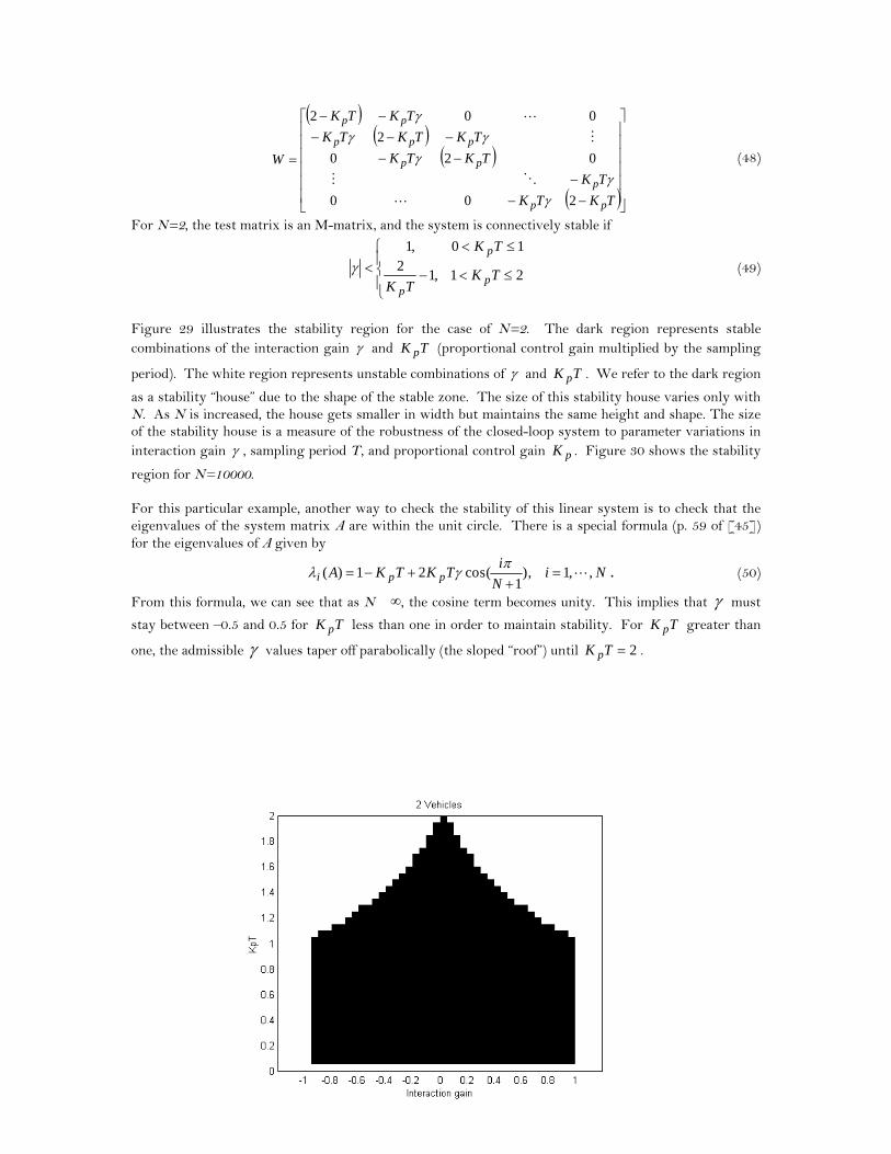
Figure 29 illustrates the stability region for the case of N=2. The dark region represents stable combinations of the interaction gain γ and (proportional control gain multiplied by the sampling

period). The white region represents unstable combinations of

TK p

γ and . We refer to the dark region

as a stability “house” due to the shape of the stable zone. The size of this stability house varies only with N. As N is increased, the house gets smaller in width but maintains the same height and shape. The size of the stability house is a measure of the robustness of the closed-loop system to parameter variations in interaction gain

TK p

γ , sampling period T, and proportional control gain . Figure 30 shows the stability

region for N=10000. pK

For this particular example, another way to check the stability of this linear system is to check that the eigenvalues of the system matrix A are within the unit circle. There is a special formula (p. 59 of [45]) for the eigenvalues of A given by

NiN

iTKTKA ppi ,,1),

1cos(21)( L=

++−=

πγλ . (50)

From this formula, we can see that as N �∞, the cosine term becomes unity. This implies that γ must

stay between –0.5 and 0.5 for less than one in order to maintain stability. For greater than

one, the admissible

TK p TK p

γ values taper off parabolically (the sloped “roof”) until 2=TK p .

39

Figure 29. Stability region for the N=2 vehicle case.

Figure 30. Stability region for the N=10000 vehicle case. Several conclusions can be drawn from this stability analysis. First, asymptotic stability of vehicle positions depends on vehicle responsiveness , communication sampling period T, and vehicle

interaction gain

pK

γ . If the vehicle is too fast (large ) or the sample period is too long (large T) then

the vehicles will go unstable. There is a dependence on interaction gain for stability as well. Second, the interaction gains can be used to bunch the vehicles closer together or spread them out. Third, the stability region shrinks as the number of vehicles, N, increases but only to a defined limit.

pK

As noted, the communication sample period greatly affects the stability of the system. As defined in the equations above, this sample period is the time it takes for every node to communicate once. In this section, we will evaluate the communication sample period of four different communication schemes: a Time Division Medium Access (TDMA) linear broadcast, a TDMA polylogarithmic broadcast, a TDMA coloring algorithm, and a Collision Sense Medium Access (CSMA) coloring algorithm. All of these schemes assume that each node has a unique identification number. The TDMA schemes also assume that each node has a synchronized clock that is used to notify each node when it may transmit a message. The CSMA scheme first checks the communication channel for a collision before transmitting a packet. In order to determine this sample period, one important parameter associated with an ad hoc communication network is the degree of the network. The degree of the network is defined as the maximum number of nodes that any node can communicate with given a limited communication range.

40

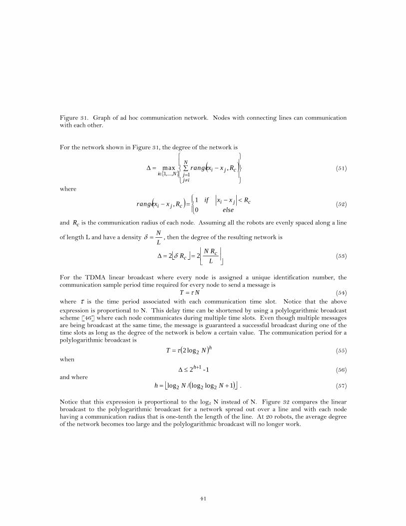
Figure 31. Graph of ad hoc communication network. Nodes with connecting lines can communication with each other. For the network shown in Figure 31, the degree of the network is

{ }(

⎪⎭

⎪⎬

⎫

⎪⎩

⎪⎨

⎧

∑ −=Δ

≠=∈

N

ijj

cjiNi

Rxxrange1,...,1

,max ) (51)

where

( )⎪⎩

⎪⎨⎧ <−=−

else

RxxifRxxrange cji

cji0

1, (52)

and is the communication radius of each node. Assuming all the robots are evenly spaced along a line

of length L and have a density

cR

L

N=δ , then the degree of the resulting network is

⎣ ⎦ ⎥⎦

⎥⎢⎣

⎢==Δ

L

RNR c

c 22 δ (53)

For the TDMA linear broadcast where every node is assigned a unique identification number, the communication sample period time required for every node to send a message is

NT τ= (54) where τ is the time period associated with each communication time slot. Notice that the above expression is proportional to N. This delay time can be shortened by using a polylogarithmic broadcast scheme [46] where each node communicates during multiple time slots. Even though multiple messages are being broadcast at the same time, the message is guaranteed a successful broadcast during one of the time slots as long as the degree of the network is below a certain value. The communication period for a polylogarithmic broadcast is

( )hNT 2log2τ= (55) when

1-2 1+≤Δ h (56) and where

( )⎣ ⎦1loglog/log 222 += NNh . (57) Notice that this expression is proportional to the log2 N instead of N. Figure 32 compares the linear broadcast to the polylogarithmic broadcast for a network spread out over a line and with each node having a communication radius that is one-tenth the length of the line. At 20 robots, the average degree of the network becomes too large and the polylogarithmic broadcast will no longer work.

41

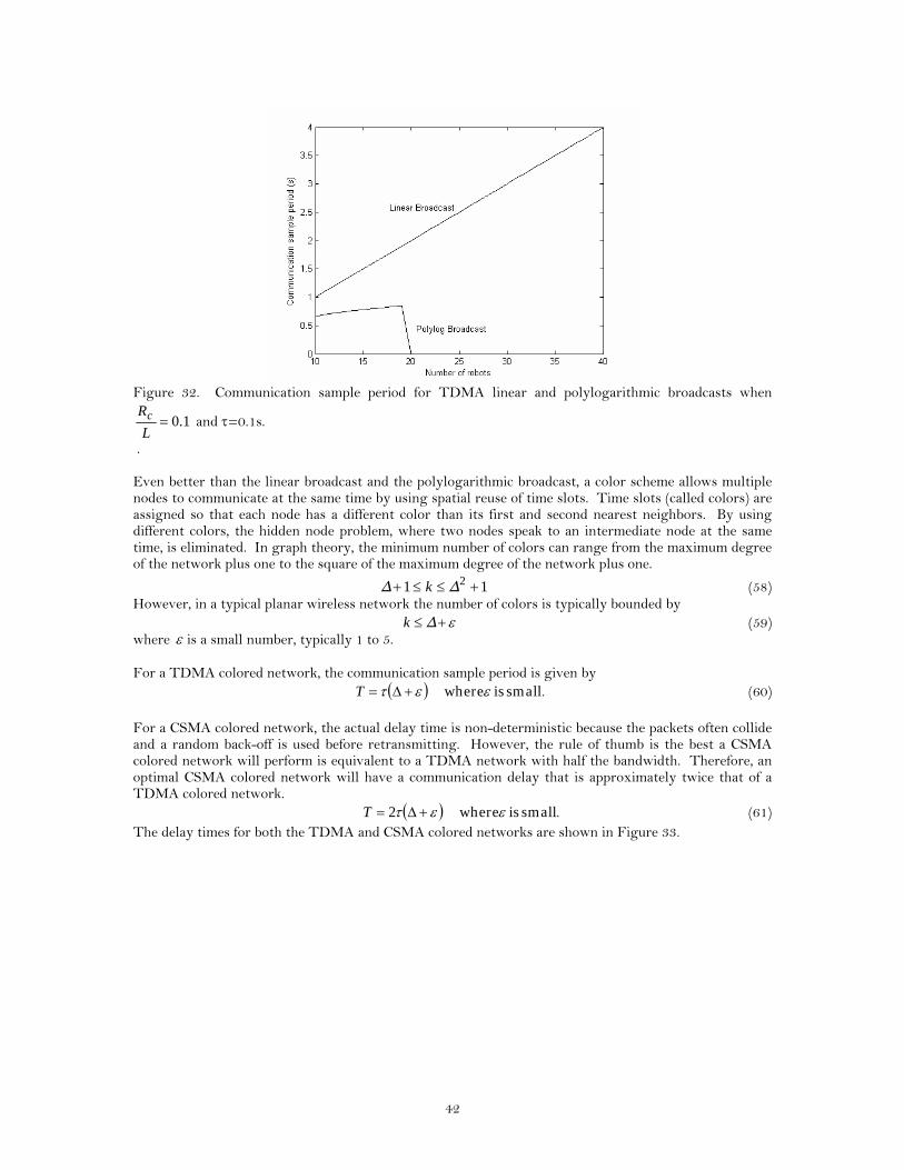
Figure 32. Communication sample period for TDMA linear and polylogarithmic broadcasts when

1.0=L

Rc and τ=0.1s.

. Even better than the linear broadcast and the polylogarithmic broadcast, a color scheme allows multiple nodes to communicate at the same time by using spatial reuse of time slots. Time slots (called colors) are assigned so that each node has a different color than its first and second nearest neighbors. By using different colors, the hidden node problem, where two nodes speak to an intermediate node at the same time, is eliminated. In graph theory, the minimum number of colors can range from the maximum degree of the network plus one to the square of the maximum degree of the network plus one.

11 2 +≤≤+ ΔkΔ (58) However, in a typical planar wireless network the number of colors is typically bounded by

ε+≤ Δk (59) where ε is a small number, typically 1 to 5. For a TDMA colored network, the communication sample period is given by

( ) small is whereεετ +Δ=T . (60) For a CSMA colored network, the actual delay time is non-deterministic because the packets often collide and a random back-off is used before retransmitting. However, the rule of thumb is the best a CSMA colored network will perform is equivalent to a TDMA network with half the bandwidth. Therefore, an optimal CSMA colored network will have a communication delay that is approximately twice that of a TDMA colored network.

( ) small is where2 εετ +Δ=T . (61) The delay times for both the TDMA and CSMA colored networks are shown in Figure 33.

42

Figure 33. Communication sample period for TDMA and CSMA reconfigurable coloring when

1.0=L

Rc , τ=0.1s,and ε=1.

Notice that both the TDMA and CSMA colored networks have a shorter communication sample period compared to both linear and polylogarithmic broadcasts. The disadvantage of the colored networks is that there is an initialization time that is required to determine the color of each node whenever the network topology changes. Both the linear broadcast and the polylogarithmic broadcast have the advantage that they do not require a network initialization time. Using an algorithm by [47], this initialization time is the time required to broadcast their own identification number, their 1st nearest neighbor lists (after which each node can determine 2nd nearest neighbor), and k+2 additional messages for coloring. Since time slots are typically not assigned before hand, this initialization process occurs using CSMA protocols, and it should be performed whenever the topology of the network changes, i.e. when robots move. The resulting initialization time is given by

( ) ( )( )[ ] 222tinit εεετ +Δ++Δ++Δ= (62)

where ε is small. This initialization time is plotted as a function of the number of robots in Figure 34. Adding the initialization time in Figure 34 to the communication sample period in Figure 33, we see that a linear or polylogarithmic broadcast has a shorter sample period than the colored network for this

particular example where 1.0=L

Rc . However, as L

Rc decreases, there is a point where the colored

networks, even with continual initialization, will out perform the linear and polylogarithmic broadcasts.

43

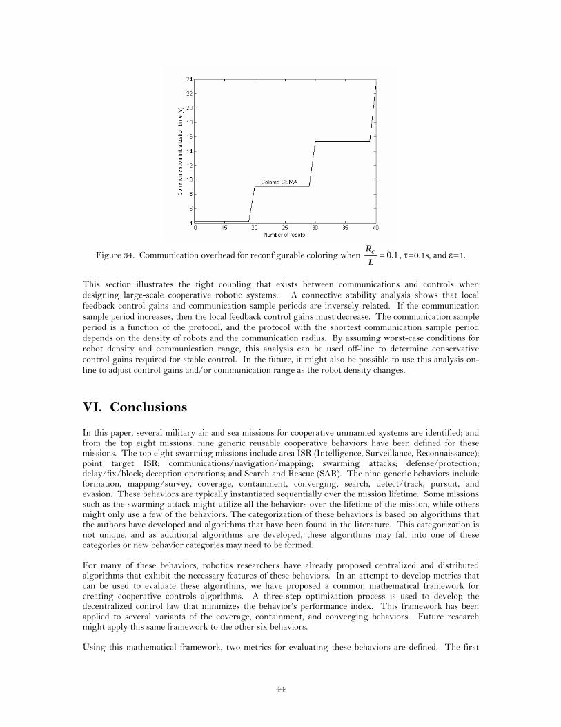
Figure 34. Communication overhead for reconfigurable coloring when 1.0=L

Rc , τ=0.1s, and ε=1.

This section illustrates the tight coupling that exists between communications and controls when designing large-scale cooperative robotic systems. A connective stability analysis shows that local feedback control gains and communication sample periods are inversely related. If the communication sample period increases, then the local feedback control gains must decrease. The communication sample period is a function of the protocol, and the protocol with the shortest communication sample period depends on the density of robots and the communication radius. By assuming worst-case conditions for robot density and communication range, this analysis can be used off-line to determine conservative control gains required for stable control. In the future, it might also be possible to use this analysis on-line to adjust control gains and/or communication range as the robot density changes. VI. Conclusions

In this paper, several military air and sea missions for cooperative unmanned systems are identified; and from the top eight missions, nine generic reusable cooperative behaviors have been defined for these missions. The top eight swarming missions include area ISR (Intelligence, Surveillance, Reconnaissance); point target ISR; communications/navigation/mapping; swarming attacks; defense/protection; delay/fix/block; deception operations; and Search and Rescue (SAR). The nine generic behaviors include formation, mapping/survey, coverage, containment, converging, search, detect/track, pursuit, and evasion. These behaviors are typically instantiated sequentially over the mission lifetime. Some missions such as the swarming attack might utilize all the behaviors over the lifetime of the mission, while others might only use a few of the behaviors. The categorization of these behaviors is based on algorithms that the authors have developed and algorithms that have been found in the literature. This categorization is not unique, and as additional algorithms are developed, these algorithms may fall into one of these categories or new behavior categories may need to be formed. For many of these behaviors, robotics researchers have already proposed centralized and distributed algorithms that exhibit the necessary features of these behaviors. In an attempt to develop metrics that can be used to evaluate these algorithms, we have proposed a common mathematical framework for creating cooperative controls algorithms. A three-step optimization process is used to develop the decentralized control law that minimizes the behavior’s performance index. This framework has been applied to several variants of the coverage, containment, and converging behaviors. Future research might apply this same framework to the other six behaviors. Using this mathematical framework, two metrics for evaluating these behaviors are defined. The first

44

metric is the residual error in the global performance index that is used to create the behavior. The second metric is communication sample period between robots, which affects the overall time required for the behavior to reach its goal state. For the second metric, a connective stability analysis is performed to determine constraints on the communication sample period and the local control gains. The communication sample period is evaluated for four different network protocols: Time Division Medium Access (TDMA) linear broadcast, a TDMA polylogarithmic broadcast, a TDMA coloring algorithm, and a Collision Sense Medium Access (CSMA) coloring algorithm. The communication sample period is a function of the protocol, and the protocol with the shortest communication sample period depends on the density of robots and the communication radius. By assuming worst-case conditions for robot density and communication range, this analysis can be used off-line to determine conservative control gains and communication sample periods required for stable control. A simple example of dispersion on a line was given in this report. Future research is needed to extend this analysis to other tasks such as dispersion in the plane. In the future, it might also be possible to use this analysis on-line to adjust control gains and/or communication range as the robot density changes. This is an area of future research. There are many other possible metrics that need to be investigated in the future. These include the algorithm’s robustness to failure, required on-board computing, and required sensing. There are also behavior-specific metrics that need further investigation. For example, the probability of detection and false alarm rates are important metrics that must be evaluated for a search behavior. The portions of the last two sections of this paper have been published in [48-49].

45

References [1] S. Edwards, Swarming on the Battlefield: Past, Present, and Future, RAND, 2000. [2] J. Arquilla & D. Ronfeldt, Swarming & The Future of Conflict, RAND, 2000. [3] H. Yamaguchi, “A Cooperative Hunting Behavior by Mobile Robot Troops,” Proceedings of the 1998

Conference on Robotics & Automation, Leuven, Belgium, May 1998, 3204-3209. [4] F.R. Noreils, “Multi-Robot Coordination for Battlefield Strategies,” Proceedings of the 1992 IEEE.RSJ

International Conference on Intelligent Robots and Systems, Raleigh, NC, July 1992, 1777-1784. [5] D. F. Hougen, M.D. Erickson, P.E. Rybski, S.A. Stoeter, M. Gini, N. Papanikolopoulos, “Autonomous

Mobile Robots and Distributed Exploratory Missions,” Distributed Autonomous Robotic Systems 4, ed. L.E. Parker, G. Bekey, J. Barhen, Springer-Verlag 2000, pp. 221-230.

[6] B. Brumitt and M. Hebert, “Experiments in Autonomous Driving with Concurrent Goals and Multiple Vehicles,” Proceedings of the 1998 International Conference on Robotics & Automation, Leuven, Belgium, May 1998, pp.1895-1902.

[7] T. Kaga, J. Starke, P. Molnar, M. Schanz, and T. Fukuda, “Dynamic Robot-Target Assignment – Dependence of Recovering from Breakdowns on the Speed of the Selection Process,” Distributed Autonomous Robotic Systems 4, ed. L.E. Parker, G. Bekey, J. Barhen, Springer-Verlag 2000, pp. 325-334.

[8] J.E. Hurtado, R.D. Robinett, C.R. Dohrmann, S.Y. Goldsmith, “Distributed Sensing and Cooperating Control for Swarms of Robotic Vehicles,” Proc. IASTED Conference Control & Applications, Honolulu, Hawaii, Aug. 12-14, 1998.

[9] J.S. Jennings, G. Whelan, W.F. Evans, “Cooperative Search and Rescue with a Team of Mobile Robotis,” Proc. IEEE International Conference of Advanced Robotics, Monterey, CA, 1997.

[10] S. Goldsmith, J. Feddema, R. Robinett, “Analysis of Decentralized Variable Structure Control for Collective Search by Mobile Robots,” SPIE98, Proc. Sensor Fusion and Decentralized Control in Robotic Systems, Boston, November 1-6, 1998.

[11] Y. Uny Cao, Alex S. Fukunaga, and Andrew B. Kahng, “Cooperative Mobile Robotics: Antecedents and Directions,” Proceedings of the 1995 IEEE/RSJ IROS Conference, 226-234.

[12] L.E. Parker, “Current State of the Art in Distributed Autonomous Mobile Robotics,” Distributed Autonomous Robotic Systems 4, ed. L.E. Parker, G. Bekey, J. Barhen, Springer-Verlag 2000, pp. 3-12.

[13] National Research Council of the National Academies, Technology Development for Army Unmanned Ground Vehicles, The National Academies Press, 2002.

[14] Swarming Entities Roadmap resulting from U.S. Joint Forces Command Joint Experimentation (J9) Swarming Conference, November 4-8, 2002.

[15] The Navy Unmanned Undersea Vehicle (UUV) Master Plan, April 20, 2000. [16] Unmanned Aerial Vehicles Roadmap,

http://www.globalsecurity.org/intell/library/reports/2001/uavr0401.htm, April 2001. [17] W.P. Hughes Jr., Fleet Tactics and Coastal Combat, 2nd Ed., Naval Institute Press, 2000. [18] R.L. Shaw, Fighter Combat: Tactics and Maneuvering, Naval Institute Press, 1985. [19] J.B. Rigdon, R.C. Brittain, J.T. Feddema, Simulation of Cooperative Net Fires, Sandia National

Laboratories Technical Report SAND2004-1385, April 2004. [20] E. Bonabeau, M. Dorigo, G. Theraulaz, Swarm Intelligence: From Natural to Artificial Systems,

Oxford University Press, 1999. [21] Q. Chen, and J.Y.S. Luh, "Coordination and Control of a Group of Small Mobile Robots,"

Proceedings of the IEEE International Conference on Robotics and Automation, Vol. 3, 1994, pp. 2315-2320.

[22] H. Yamaguchi, and T. Arai, "Distributed and Autonomous Control Method for Generating Shape of Multiple Mobile Robot Group," Proceedings of the IEEE International Conference on Intelligent Robots and Systems, Vol. 2, 1994, pp.800-807.

[23] H. Yamaguchi, J.W. Burdick, “Asymptotic Stabilization of Multiple Nonholonomic Mobile Robots Forming Group Formations,” Proceedings of the 1998 Conference on Robotics & Automation, Leuven, Belgium, May 1998, 3573-3580.

[24] F. E. Schneider, D. Wildermuth, H.-L. Wolf, “Motion Coordination in Formations of Multiple Robots Using a Potential Field Approach,” Distributed Autonomous Robotic Systems 4, ed. L.E. Parker, G. Bekey, J. Barhen, Springer-Verlag 2000, pp. 305-314.

46

[25] J.P. Desai, V. Kumar, J.P. Ostrowski, “Modeling and Control of Formations of Nonholonomic Mobile Robots,” IEEE Transactions on Robotics and Automation, Vol. 17, No. 6, December 2001, pp. 905-908.

[26] International Aeronautical and Maritime Search and Rescue (IAMSAR) Manual, Volume III (Mobile Facilities), ICAO Publications, 1998.

[27] D. Fox, W. Burgard, H. Kruppa, and S. Thrun, “A Probabilistic Approach to Collaborative Multirobot Localization,” Autonomous Robots, Vol. 8, No. 3, pp. 325-344, 2000.

[28] M. DiMarco, A. Garulli, A. Giannitrapani, and A. Vicino, “Simultaneous Localization and Map Building for a Team of Cooperating Robots: A Set Membership Approach,” IEEE Transactions on Robotics and Automation, Vol. 19, No. 2, April 2003, pp. 238-249.

[29] S. Thrun, C. Martin, Y. Liu, D. Hahnel, R. Emery-Montemerlo, D. Chakrabarti, and W. Burgard, “A Real-Time Expectation-Maximization Algorithm for Acquiring Multiplanar Maps of Indoor Environments with Mobile Robots, IEEE Transactions on Robotics and Automation, Vol. 20, No. 3, June 2004, pp. 433-442.

[30] A.G.O. Mutambara, Decentralized Estimation and Control for Multisensor Systems, CRC Press, 1998. [31] R. Vidal, O. Shakernia, H.J. Kim, D.H. Shim, and S. Sastry, “Probabilistic Pursuit-Evasion

Games: Theory, Implementation, and Experimental Evaluation, IEEE Transactions on Robotics and Automation, Vo. 18, No. 5, pp. 662-669.

[32] B.R. Frieden, Physics from Fisher Information, Cambridge University Press, 1998. [33] Y. Censor, S.A. Zenios, Parallel Optimization: Theory, Algorithms, and Applications, Oxford

University Press, 1997. [34] D.G. Luenberger, Linear and Nonlinear Programming, 2nd Edition, Addison Wesley Publishing

Company, 1984. [35] J.T. Feddema, C. Lewis, D.A. Schoenwald, “Decentralized Control of Cooperative Robotic

Vehicles: Theory and Application,” IEEE Transactions on Robotics and Automation, Vo. 18, No. 5, pp. 852-864.

[36] C. Lewis, J.T. Feddema, P. Klarer, “Robotic Perimeter Detection System,” Proceedings of SPIE Vol. 3577, Boston, MA, November 3-5, 1998, pp. 14-21.

[37] D.J. Schmitt, et. al., “Intelligent Mobile Land Mine (IMLM) System, Sandia National Laboratories Report SAND2003-1186, July 2003.

[38] J.T. Feddema, D.A. Schoenwald, “Stability Analysis of Decentralized Cooperative Controls,” Multi-Robot Systems: From Swarms to Intelligent Automata, ed. A.C. Shultz and L.E. Parker, Kluwer Academic Publishers, pp. 133-122, 2002.

[39] J.T. Feddema, D.A. Schoenwald, “Distributed Communication/Navigation Robot Vehicle Network,” Proceedings of World Automation Congress, Orlando, Florida, June 9-13, 2002.

[40] R.D. Robinett III, J.E. Hurtado, “Stability and Control of Collective Systems,” Proceedings of John L. Junkins Astrodynamics Symposium, College Station, Texas, May 23-24, 2003.

[41] R.H. Byrne, D.R. Adkins, S.E. Eskridge, J.J. Harrington, E.J. Heller, J.E. Hurtado, “Miniature Mobile Robots for Plume Tracking and Source Localization Research,” Journal of Micromechatronics, Vol. 1, No. 3, pp. 253-261, 2002.

[42] R.H. Byrne, S.E. Eskridge, J.E. Hurtado, E.L. Salvage, “Algorithms and Analysis of Underwater Vehicle Plume Tracing,” Sandia National Laboratories Report SAND2003-2643, July 2003.

[43] D. D. Siljak, Decentralized Control of Complex Systems, Academic Press, 1991. [44] M.E. Sezer and D.D. Siljak, “Robust Stability of Discrete Systems,” Int. J. Control, Vol. 48, No. 5,

pp. 2055-2063, 1988. [45] G. D. Smith, Numerical Solution of Partial Differential Equations: Finite Difference Methods, Third

Edition, Oxford University Press, 1985. [46] S. Basagni, D. Bruschi, and I. Chlamtac, “A Mobility-Transparent Deterministic Broadcast

Mechanism for Ad Hoc Networks,” IEEE/ACM Transactions on Networks, Vol. 7, No. 6, December 1999, pp. 799-807.

[47] I. Chlamtac and S.S. Pinter, “Distributed Nodes Organization Algorithm for Channel Access in a Multihop Dynamic Radio Network,” IEEE Transactions on Computers, Vol. C-36, No. 6, June 1987, pp. 728-737.

[48] J.T. Feddema, R.D. Robinett, R.H. Byrne, “An Optimization Approach to Distributed Controls of Multiple Robotic Vehicles,” IEEE/RSJ International Conference on Intelligent Robots and Systems, Workshop on Control and Cooperation of Intelligent Miniature Robots, Las Vegas, Nevada, October 31, 2003.

47

[49] J.T. Feddema, “Communication and Control of Large Scale Cooperative Systems,” Proc. Of the American Nuclear Society 10th International Conference on Robotics and Remote Systems for Hazardous Environments, Gainesville, Florida, March 28-31, 2004.

48

Distribution 1 Dr. Douglas Gage DARPA Information Processing Technology Office 3701 North Fairfax Drive Alexandria, VA 22203-1714 1 Judith Hase Judd Science & Technology Associates 4100 Fairfax Drive, Suite 910 Alexandria, VA 22203 1 MS1002 Philip Heermann, 15230 10 MS1003 John Feddema, 15211 5 MS1003 Ray Byrne, 15211 1 MS1004 Ray Harrigan, 15221 1 MS1005 Kelly Jorgensen, 15222 1 MS1125 Phil Bennett, 15252 1 MS1007 Larry Shipers, 15272 1 MS1010 Steve Roehrig, 15200 5 MS0741 Rush Robinett, 6200 1 MS9018 Central Technical Files, 8945-1 2 MS0899 Technical Library, 9616

49

Military Airborne and Maritime Application for …prod.sandia.gov/techlib/access-control.cgi/2004/044764.pdf · Military Airborne and Maritime Application for Cooperative Behaviors

Documents