Microscopic picture – change in charge density when field is applied 3). Dielectric phenomena E (r) Change in electronic charge density Note dipolar.

• Microscopic picture – change in charge density when field is applied

3). Dielectric phenomena

E

(r) Change in electronic charge density

Note dipolar character

r

No E fieldE field on

- +

(r) Electronic charge density

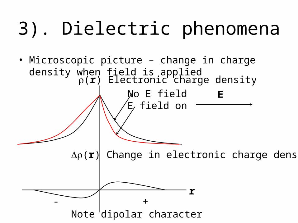
Dipole Moments of Atoms• Total electronic charge per atom

Z = atomic number

• Total nuclear charge per atom

• Centre of mass of electric or nuclear charge distribution

• Dipole moment Zea

space all

el )d( Ze rr

0 if d )(

d )()( Ze a Ze

nucspace all

el

space all

elnucelnuc

rrrr

rrrrrr

space all

nuc )d( Ze rr

space all

el/nuc

space all

el/nuc

el/nuc )d(

d )(

rr

rrr

r

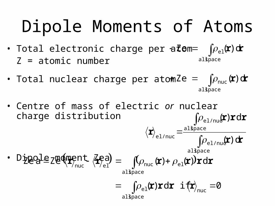
Electrostatic potential of point dipole• +/- charges, equal magnitude, q, separation a• axially symmetric potential (z axis)

a/2

a/2

r+

r-rq+

q-

x

z

p

-o

r1

r1

4

q)(

r

2

o2

o

2

2

22

222

r4

cos p

r

cos

4

qa

cos2r

a

r

1

21

cos r

a

2r

a1r

r

1

cos r

a

2r

a1r

cos r a2

arr

r

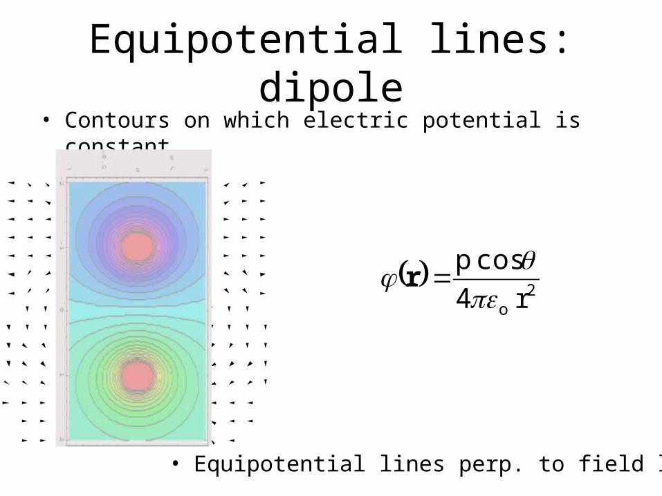
Equipotential lines: dipole• Contours on which electric potential is constant

2

o r4

cos p

r

• Equipotential lines perp. to field lines

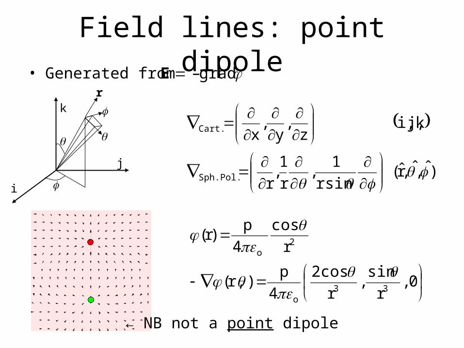
Field lines: point dipole• Generated from

),,r( sin r

1,

r

1,

r

kj,i, z

,y

,x

Sph.Pol.

Cart.

ˆˆˆ

0,,)(

)(

r

sin

r

2cos

4

pr,

r

cos

4

pr

33o

2o

r

i

j

k

grad – E

← NB not a point dipole

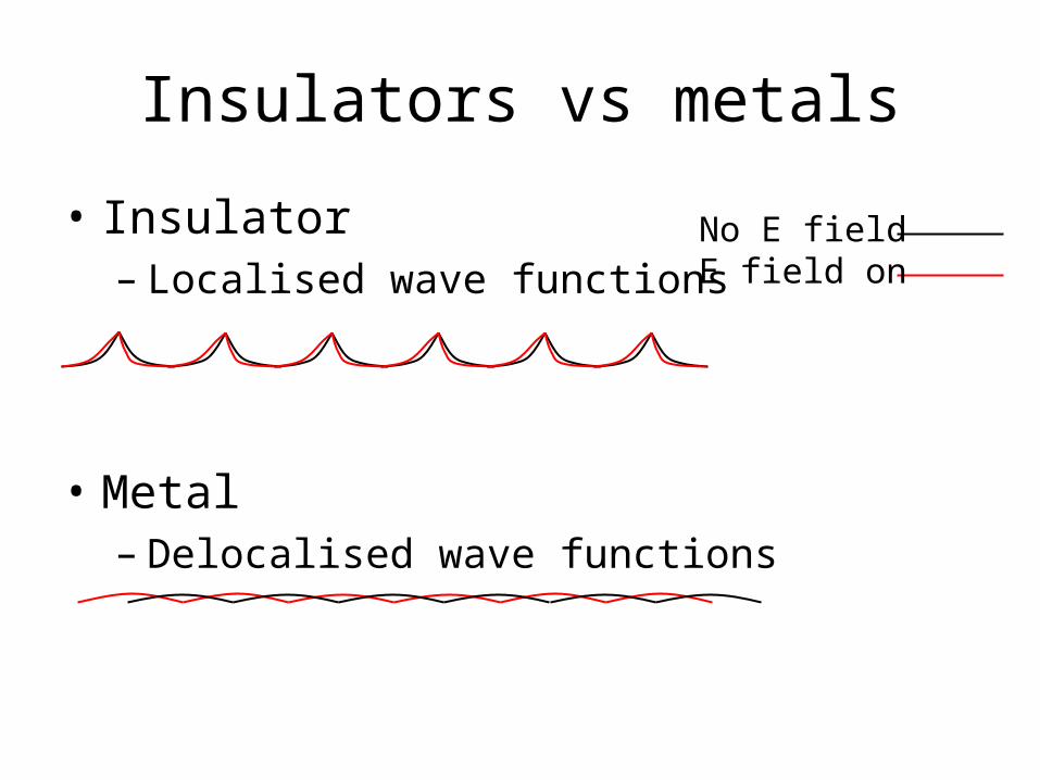
Insulators vs metals

• Insulator– Localised wave functions

• Metal– Delocalised wave functions

No E fieldE field on

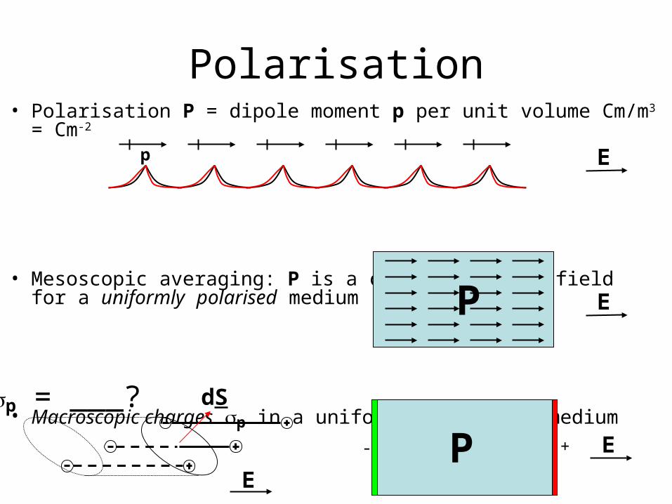
• Polarisation P = dipole moment p per unit volume Cm/m3 = Cm-2

• Mesoscopic averaging: P is a constant vector field for a uniformly polarised medium

• Macroscopic charges p in a uniformly polarised medium

Polarisation

P- +

p E

P E

E

dS

E

p = ___?

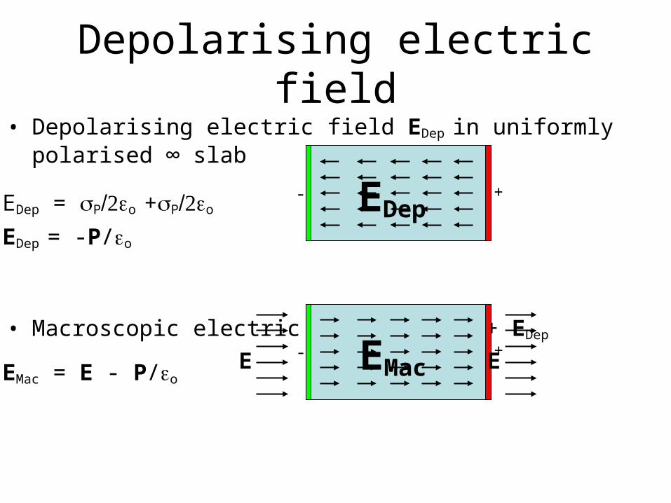
Depolarising electric field• Depolarising electric field EDep in uniformly polarised ∞ slab

• Macroscopic electric field EMac= E + EDep

EDep- +

EMac- +EE

EDep = Po +Po

EDep = -P/o

EMac = E - P/o

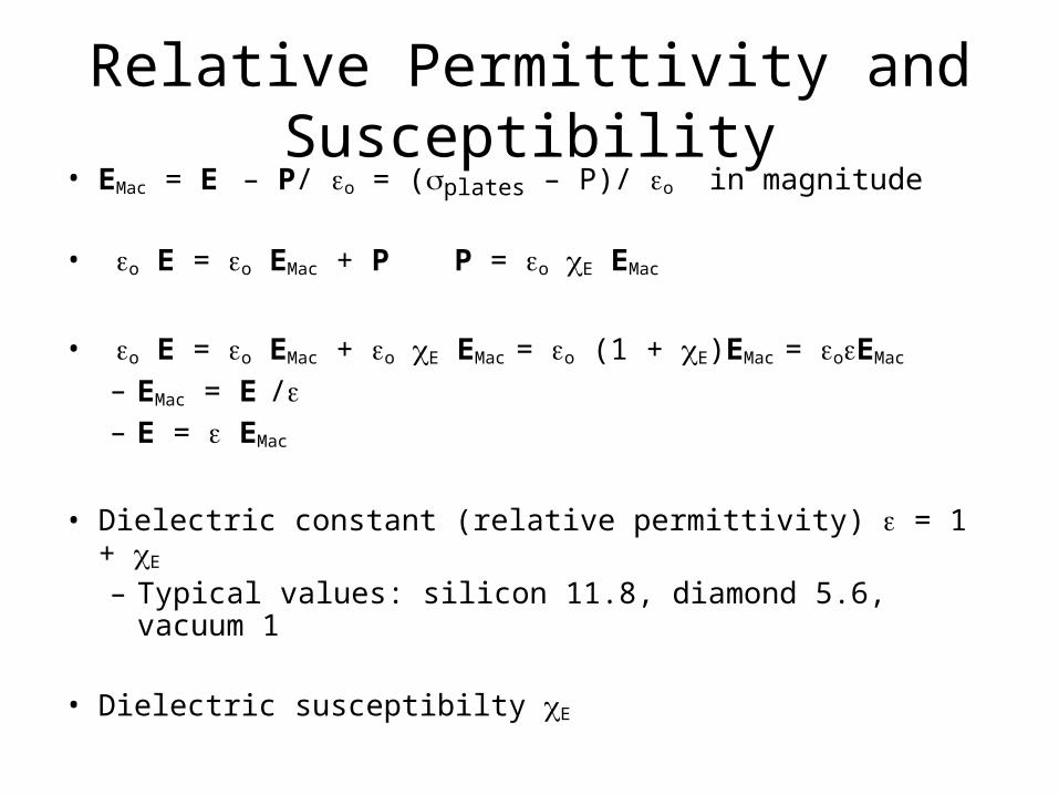
Relative Permittivity and Susceptibility• EMac = E – P/ o = (plates – P)/ o in magnitude • o E = o EMac + P P = o E EMac

• o E = o EMac + o E EMac = o (1 + E)EMac = oEMac

– EMac = E /– E = EMac

• Dielectric constant (relative permittivity) = 1 + E

– Typical values: silicon 11.8, diamond 5.6, vacuum 1

• Dielectric susceptibilty E

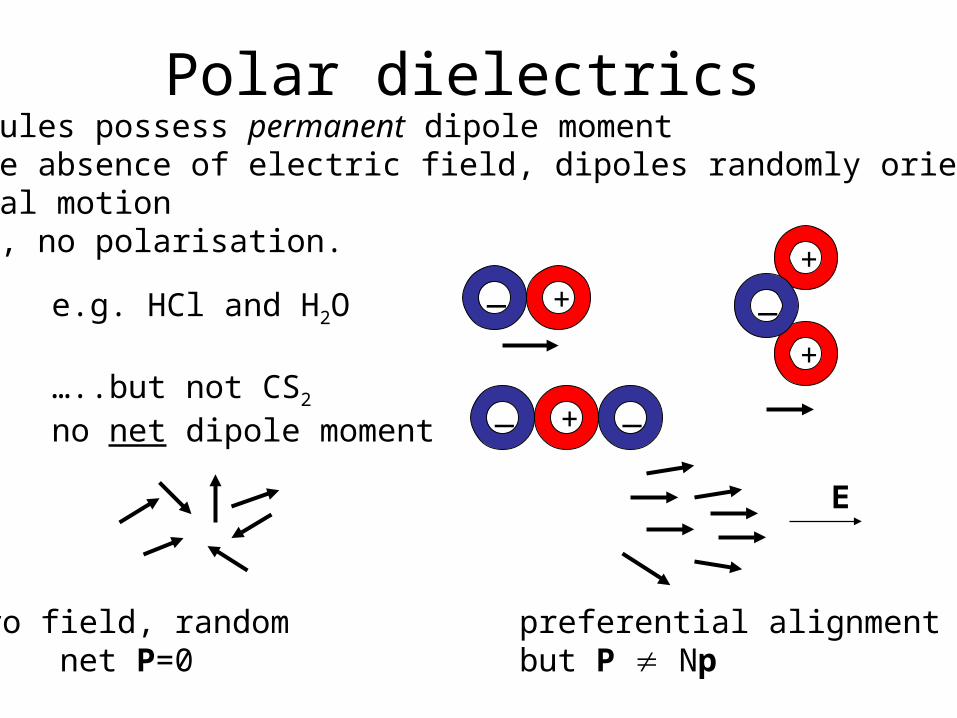
Polar dielectrics• molecules possess permanent dipole moment • in the absence of electric field, dipoles randomly oriented by

thermal motion• hence, no polarisation.

e.g. HCl and H2O

…..but not CS2

no net dipole moment

+

+

+

+_

__

_

E

zero field, random preferential alignment net P=0 but P Np

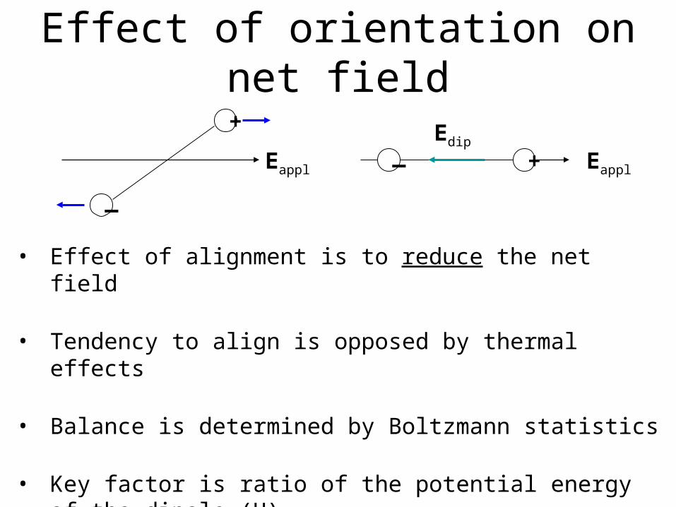
Effect of orientation on net field

• Effect of alignment is to reduce the net field

• Tendency to align is opposed by thermal effects

• Balance is determined by Boltzmann statistics

• Key factor is ratio of the potential energy of the dipole (U) to the temperature (T), which enters as exp(-U/kT)

Eappl + _ Eappl

_

+ Edip

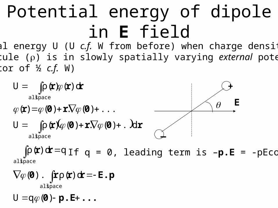
Potential energy of dipole in E field• Potential energy U (U c.f. W from before) when charge density

of molecule () is in slowly spatially varying external potential(No factor of ½ c.f. W)

E

_

+

...p.E0

E.prr r0

rr

r0r0r

0r0r

rrr

)(qU

)dρ().(

q)dρ(

d...)(.)()ρ(U

...)(.)()(

)d()ρ(U

space all

space all

space all

space all

If q = 0, leading term is –p.E = -pEcos

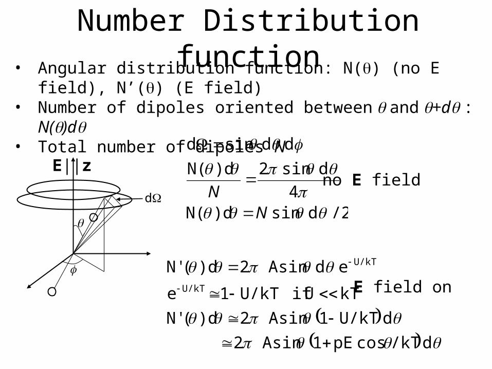
Number Distribution function• Angular distribution function: N() (no E field), N’() (E field)• Number of dipoles oriented between and +d : N()d• Total number of dipoles N

/2d sin )dN(4

d sin 2)dN(

dd sind

NN

d /kTcos pE1 sin A 2

d U/kT1 sin A 2)d(N'

kTU if U/kT1e

e d sin A 2)d(N'U/kT

U/kT

d

E||zno E field

E field on

• Total number of dipoles N

Number Distribution function

4 / A

A4)d(N'

kT

d cos sin pE A 2d sin A 2)d(N'

)d(N'

π

0

π

0

N

N

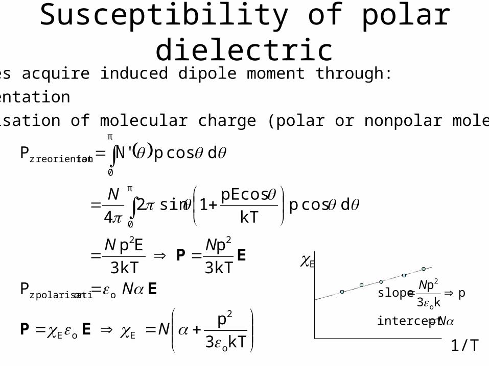
Susceptibility of polar dielectric

kT3

p

P

3kT

p

3kT

Ep

d cos p kT

pEcos1 sin 2

4

d cos p N'P

o

2

EoE

oonpolarisati z

22

π

0

π

0

ionreorientat z

N

N

N N

N

E P

E

EP

• Molecules acquire induced dipole moment through:

- reorientation

- polarisation of molecular charge (polar or nonpolar molecules)

E

1/T

N

N

intercept

p k3

pslope

o

2

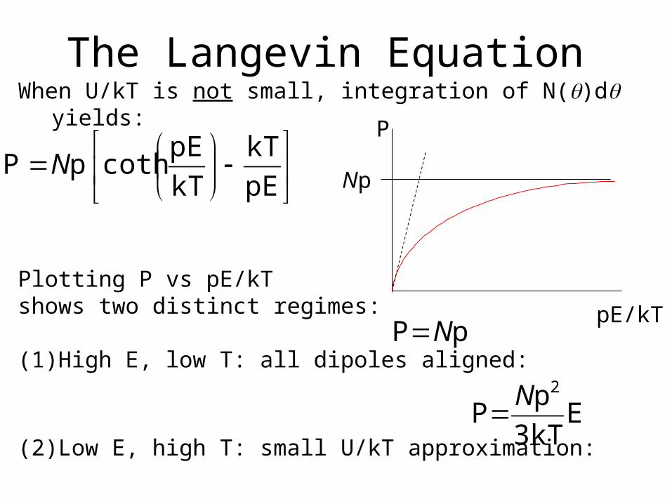
The Langevin Equation When U/kT is not small, integration of N()d yields:

Plotting P vs pE/kTshows two distinct regimes:

(1) High E, low T: all dipoles aligned:

(2) Low E, high T: small U/kT approximation: E3kT

pP

2N

pE

kT

kT

pEcoth pP N

pP N

pE/kT

Np

P

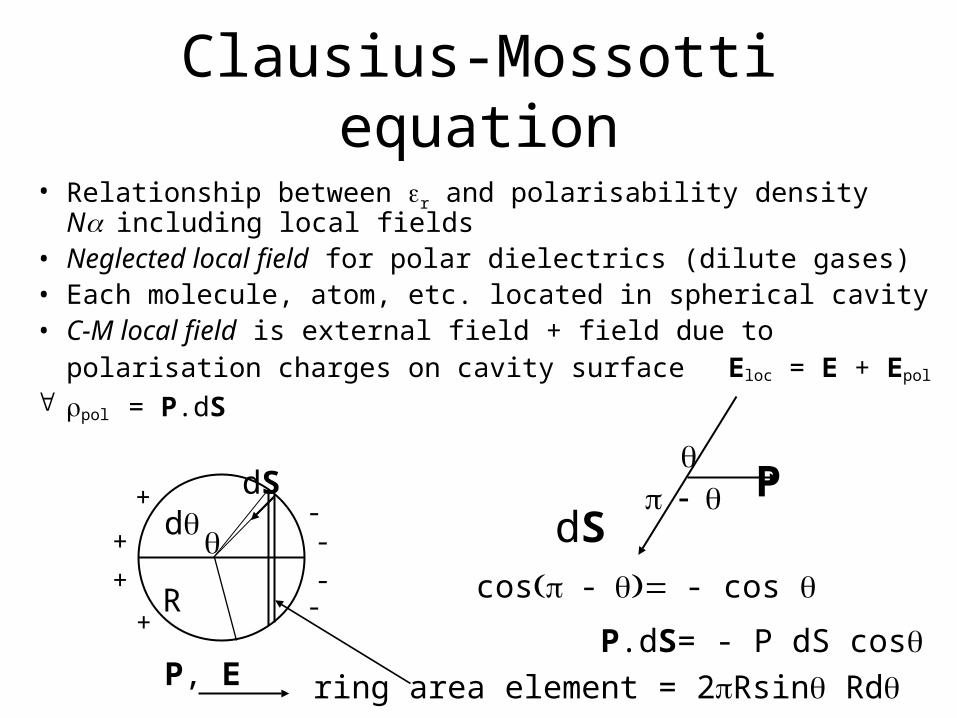
Clausius-Mossotti equation

• Relationship between r and polarisability density Nincluding local fields

• Neglected local field for polar dielectrics (dilute gases)• Each molecule, atom, etc. located in spherical cavity• C-M local field is external field + field due to polarisation

charges on cavity surface Eloc = E + Epol

pol = P.dS

d

R

P, E

dS

-

-

-

-

+

+

+

+

cos-- cos

P.dS= - P dS cosring area element = 2Rsin Rd

PdS

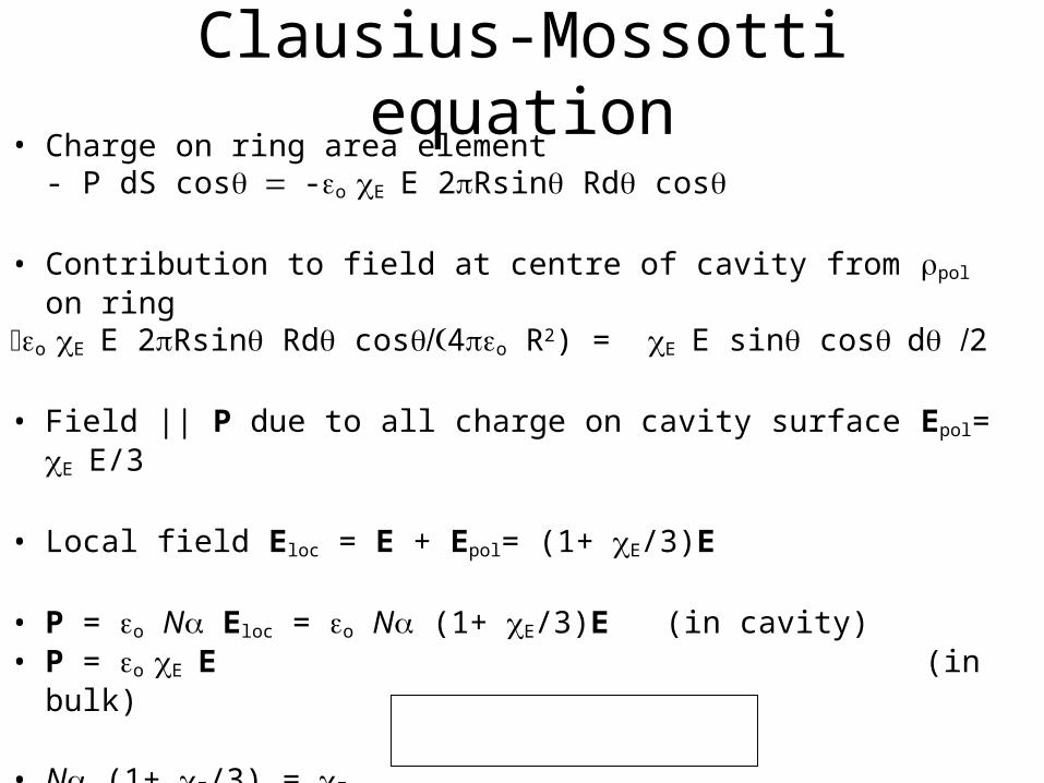
Clausius-Mossotti equation• Charge on ring area element

- P dS cos-o EE 2Rsin Rd cos

• Contribution to field at centre of cavity from pol on ringo EE 2Rsin Rd cos4o R2) = EE sin cosd 2

• Field || P due to all charge on cavity surface Epol= EE/3

• Local field Eloc = E + Epol= (1+ E/3)E

• P = o N Eloc = o N (1+ E/3)E (in cavity)• P = o EE (in bulk)

• N (1+ E/3) = E• N = E / (1+ E/3) N/3 = (r – 1)/(r + 2) since r = 1 + E

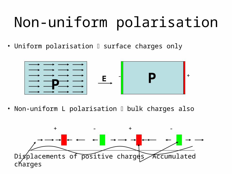
Non-uniform polarisation

• Uniform polarisation surface charges only

• Non-uniform L polarisation bulk charges also

Displacements of positive charges Accumulated charges

P- +

PE

+ +- -

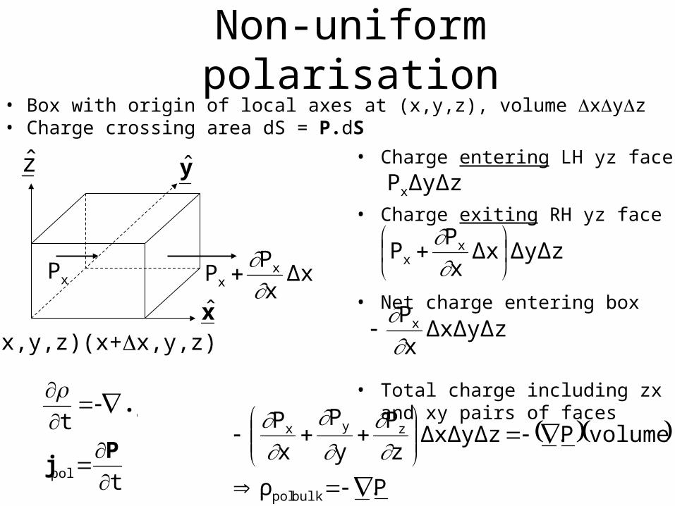
Non-uniform polarisation• Box with origin of local axes at (x,y,z), volume xyz • Charge crossing area dS = P.dS

(x,y,z)x

yz

(x+x,y,z)

Δxx

PP x

x

xP

• Charge entering LH yz face

• Charge exiting RH yz face

• Net charge entering box

• Total charge including zx and xy pairs of faces

ΔyΔzPx

ΔxΔyΔzx

Px

P.ρ

volumeP.ΔxΔyΔzz

P

y

P

x

P

bulk pol

zyx

ΔyΔzΔxx

PP x

x

t

t

pol

Pj

.j

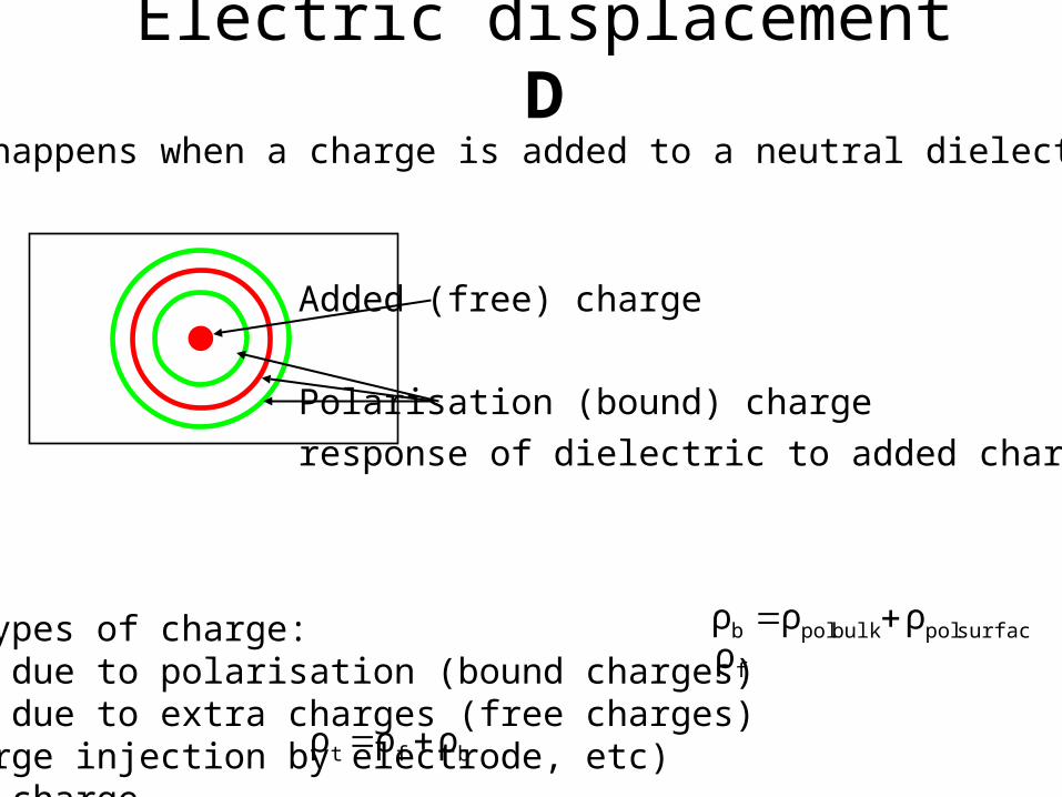
Electric displacement D• What happens when a charge is added to a neutral dielectric ?

• Two types of charge: • Those due to polarisation (bound charges)• Those due to extra charges (free charges) (charge injection by electrode, etc)• Total charge

Added (free) charge

Polarisation (bound) charge

response of dielectric to added charge

fρsurface polbulk polb ρρρ

bft ρρρ

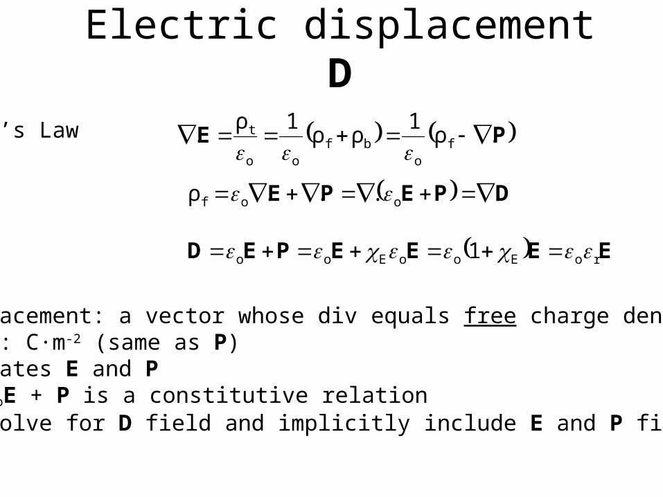
Electric displacement D

• Gauss’s Law

• Displacement: a vector whose div equals free charge density• Units: C·m-2 (same as P)• D relates E and P• D = oE + P is a constitutive relation• Can solve for D field and implicitly include E and P fields

PE .ρ1

ρρ1ρ

. fo

bfoo

t

EEEEPED roEooEoo 1

DPEPE ....ρ oof

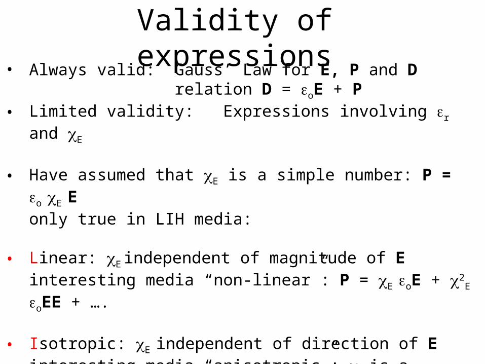
Validity of expressions• Always valid: Gauss’ Law for E, P and D

relation D = oE + P• Limited validity: Expressions involving r and E

• Have assumed that E is a simple number: P = o E Eonly true in LIH media:

• Linear: E independent of magnitude of E interesting media “non-linear”: P = E oE + 2

E oEE + ….

• Isotropic: E independent of direction of E interesting media “anisotropic”: E is a tensor (generates vector)

• Homogeneous: uniform medium (spatially varying r)

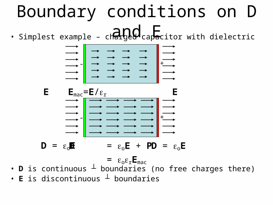
Boundary conditions on D and E• Simplest example – charged capacitor with dielectric

• D is continuous ┴ boundaries (no free charges there)• E is discontinuous ┴ boundaries

- +

D = oE D = oE + P

= orEmac

D = oE

- +

E Emac=E/r E

Boundary conditions on D• We know that

• Absence of free charges at boundaryD1 cos1 S – D2 cos2 S = 0D1 cos1 = D2 cos2

D1┴ = D2 ┴

Perpendicular component of D is continuous

• Presence of free charges at boundaryD1 cos1 S – D2 cos2 S = S f

D1┴ = D2 ┴

+ f

Discontinuity in perpendicular component of D is free charge areal density

dv.ddvv

f

Sv

f

SD D

D

.

.

0 S

.dSD

dv.dv

f

S SD

1

2

(E1,D1)

(E2,D2)2

1

S

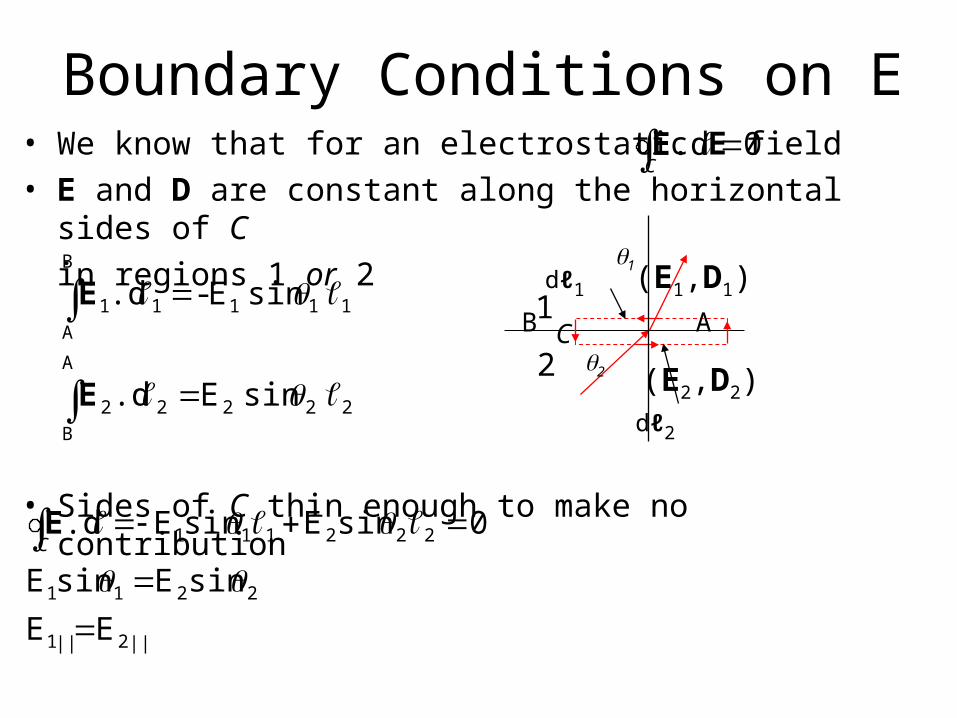
Boundary Conditions on E• We know that for an electrostatic E field• E and D are constant along the horizontal sides of C

in regions 1 or 2

• Sides of C thin enough to make no contribution

• Parallel component of E is continuous across boundary

0.d C E

222

A

B

22

111

B

A

11

sin E .d

sin E- .d

E

E 1

2 (E2,D2)

(E1,D1)

2

1dℓ1

dℓ2

C AB

||||

0

21

2211

222111

EE

sinEsinE

sinEsinE.d

CE

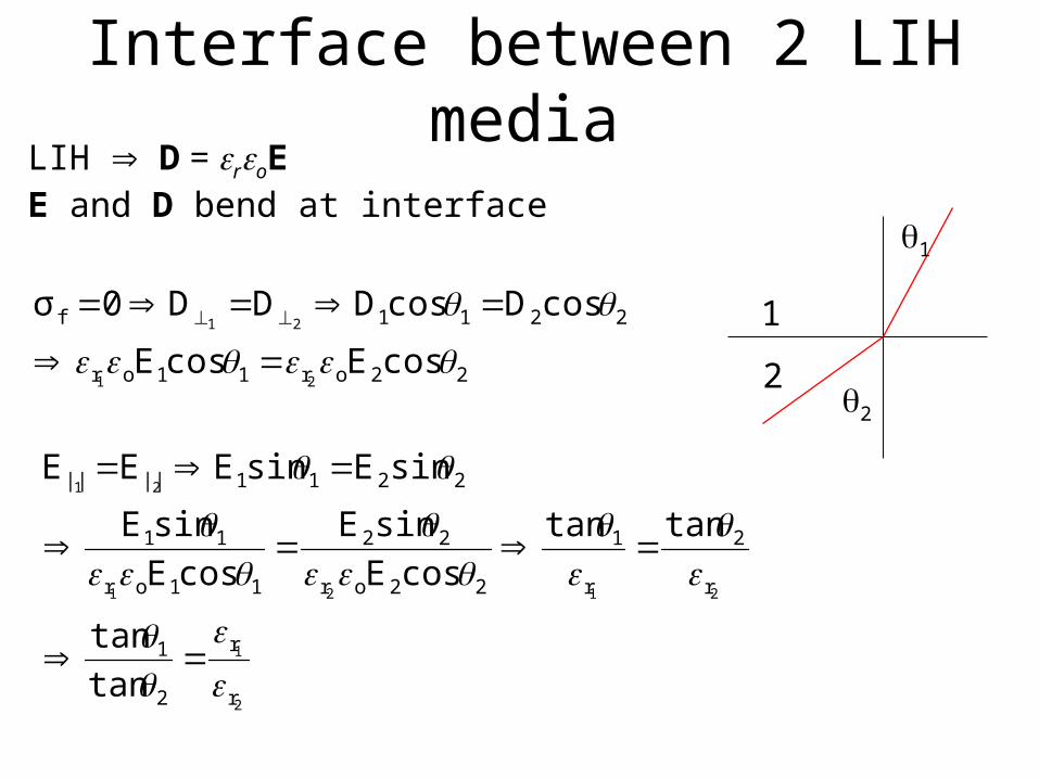
Interface between 2 LIH mediaLIH D = roEE and D bend at interface

22or11or

2211f

cosEcosE

cosDcosDDD0σ

21

21

2

1

2121

21

r

r

2

1

r

2

r

1

22or

22

11or

11

2211||||

tan

tan

tantan

cosE

sinE

cosE

sinE

sinEsinEEE

1

2

1

2

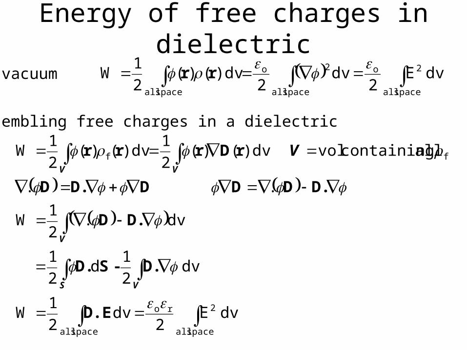
Energy of free charges in dielectric

space all

2o

space all

2o

space all

dvE2

dv2

)dv()(2

1W

rr• In vacuum

• Assembling free charges in a dielectric

dv E2

dv 2

1W

dv 2

1d

2

1

dv.2

1W

....

all containing vol )dv(.)(2

1)dv()(

2

1W

space all

2ro

space all

f

f

D.E

D.- SD.

D.D

D.DD DD.D

rDrrr

S V

V

VV

V

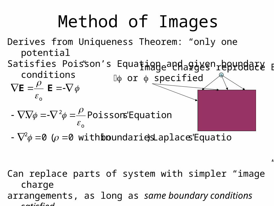
Method of ImagesDerives from Uniqueness Theorem: “only one potential Satisfies Poisson’s Equation and given boundary conditions”

Can replace parts of system with simpler “image” charge arrangements, as long as same boundary conditions satisfiedMethod exploits:

(1) Symmetry(2) Gauss’s Law

Equation sLaplace'boundaries within0

Equation sPoisson'.

.

o

o

)( 0

2

2

EE or specified

Image charges reproduce BC

Basic Image Charge ExampleConsider a point charge near an infinite, grounded, conducting plate: induced -ve charge on plate; potential zero at plate surface

Complex field pattern, combining radial (point charge +Q) and planar (conducting plate) symmetries, can also be viewed as half of pattern of 2 point charges (+Q and -Q)of equal magnitude and opposite sign!

+Q +Q -Q

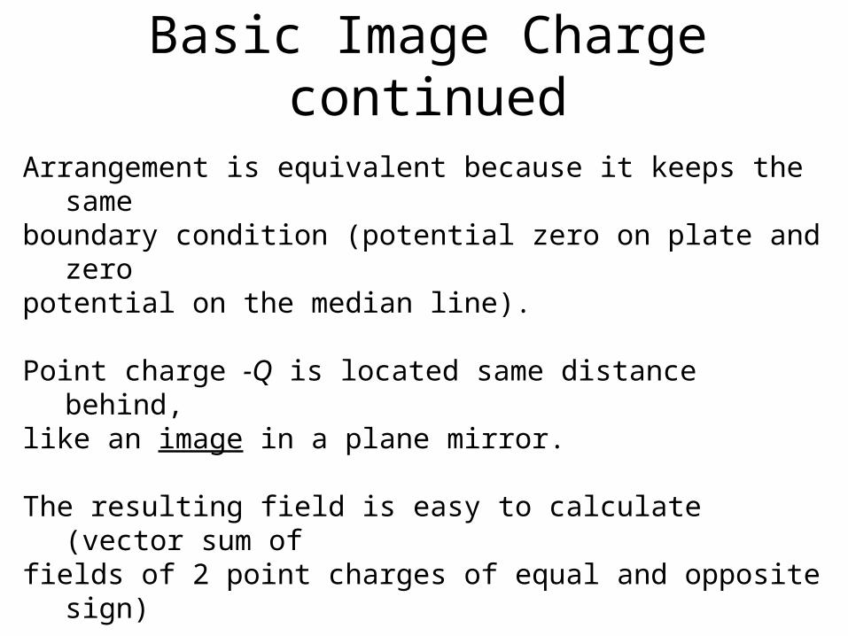
Basic Image Charge continued

Arrangement is equivalent because it keeps the same boundary condition (potential zero on plate and zero potential on the median line).

Point charge -Q is located same distance behind, like an image in a plane mirror.

The resulting field is easy to calculate (vector sum of fields of 2 point charges of equal and opposite sign)

Field lines must be normal to surface of conductor

Also easy to calculate the induced -ve charge on plate!

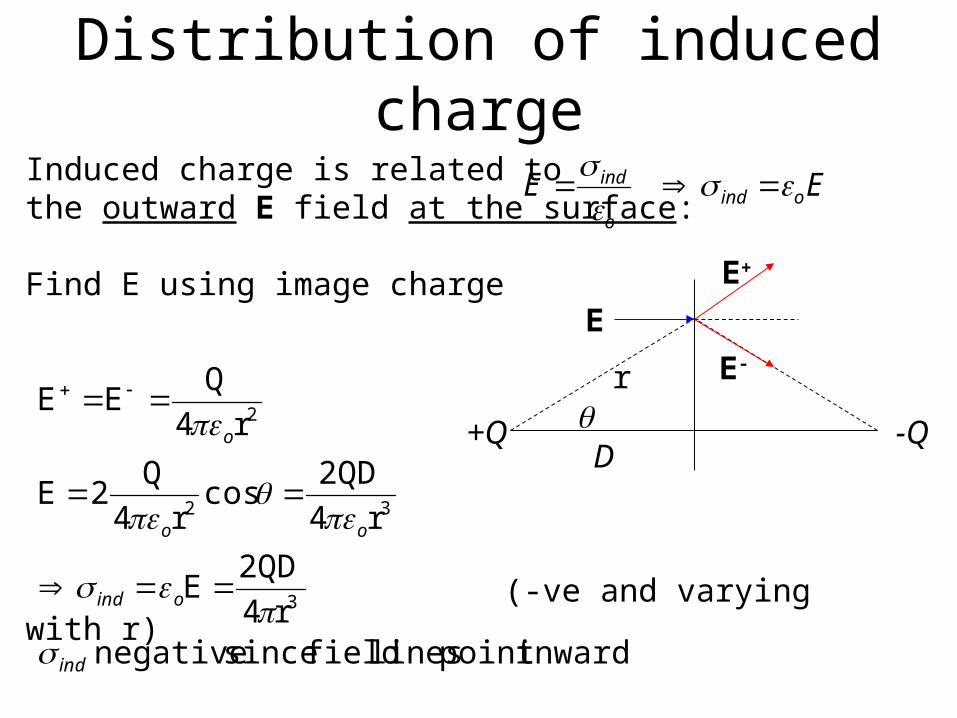
Distribution of induced charge

Induced charge is related to the outward E field at the surface:

Find E using image charge

(-ve and varying with r)

E ind

o

ind oE

inwards point lines field since negative r

2QDE

r

2QDcos

r

QE

r

QEE

3

32

2

ind

oind

oo

o

4

442

4

D+Q -Q

E

E+

E-

r

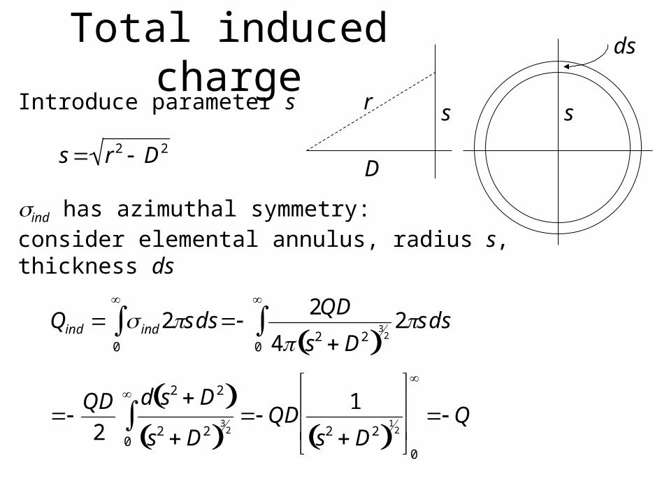
Total induced chargeIntroduce parameter s

ind has azimuthal symmetry:consider elemental annulus, radius s, thickness ds

s r2 D2

Qind ind 2sds0

2QD

4 s2 D2 3

22sds

0

QD

2

d s2 D2 s2 D2

32QD

1

s2 D2 1

2

0

0

Q

ds

r

D

s s

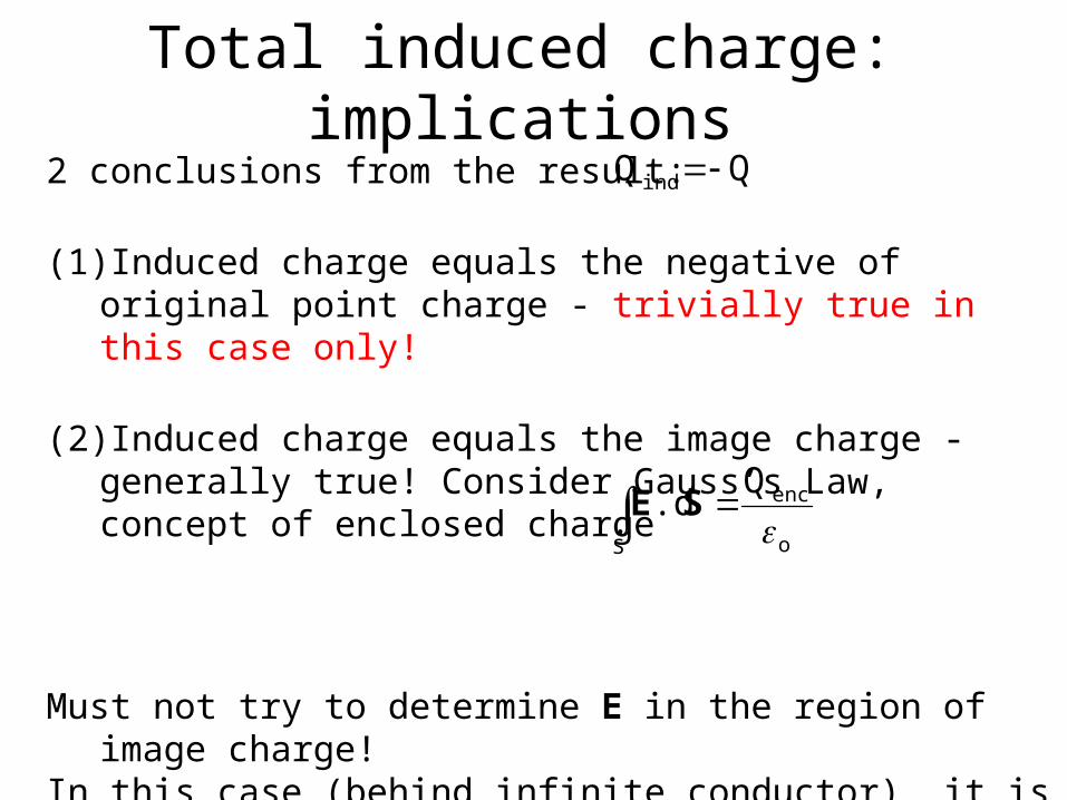
Total induced charge: implications2 conclusions from the result:

(1) Induced charge equals the negative of original point charge - trivially true in this case only!

(2) Induced charge equals the image charge - generally true! Consider Gauss’s Law, concept of enclosed charge

Must not try to determine E in the region of image charge!In this case (behind infinite conductor) it is zero, which is not the answer the image charge would yield

QQind

S o

encQ.d

SE

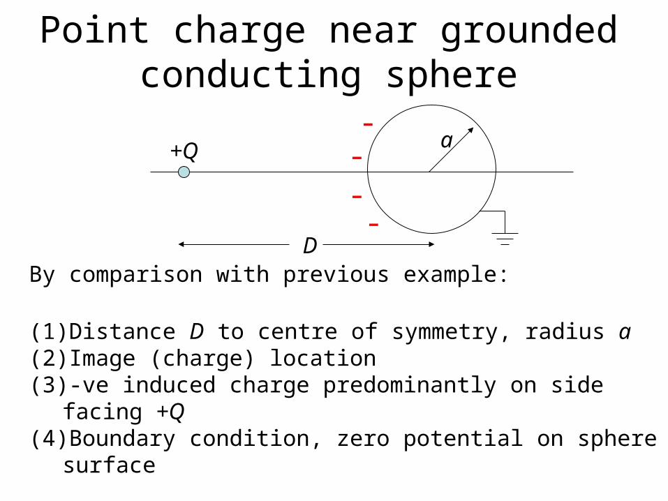
Point charge near grounded conducting sphere

By comparison with previous example:

(1) Distance D to centre of symmetry, radius a(2) Image (charge) location(3) -ve induced charge predominantly on side facing +Q(4) Boundary condition, zero potential on sphere surface

Expect image charge will be a point charge on centre line,left of centre of sphere, magnitude not equal to Q, call it Q

D

+Q a-

---

Point charge near grounded conducting sphere

Q distance b from centre, =0 at symmetry points P1 and P2

Q

D

P2 P1Q

b

Gauss by Q'Q DaQ' and D

ab solving

P at

P at

ind

2

2

1

04

1

04

1

ba

Q

aD

Q

ba

Q

aD

Q

o

o

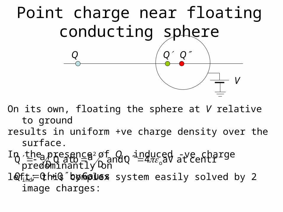
Point charge near floating conducting sphere

On its own, floating the sphere at V relative to ground results in uniform +ve charge density over the surface.In the presence of Q, induced -ve charge predominantly on left; this complex system easily solved by 2 image charges:

Gaussby QQ Q

centre ataV 4Qand Dab at QD

aQ

ind

o

2

Q

V

Q Q

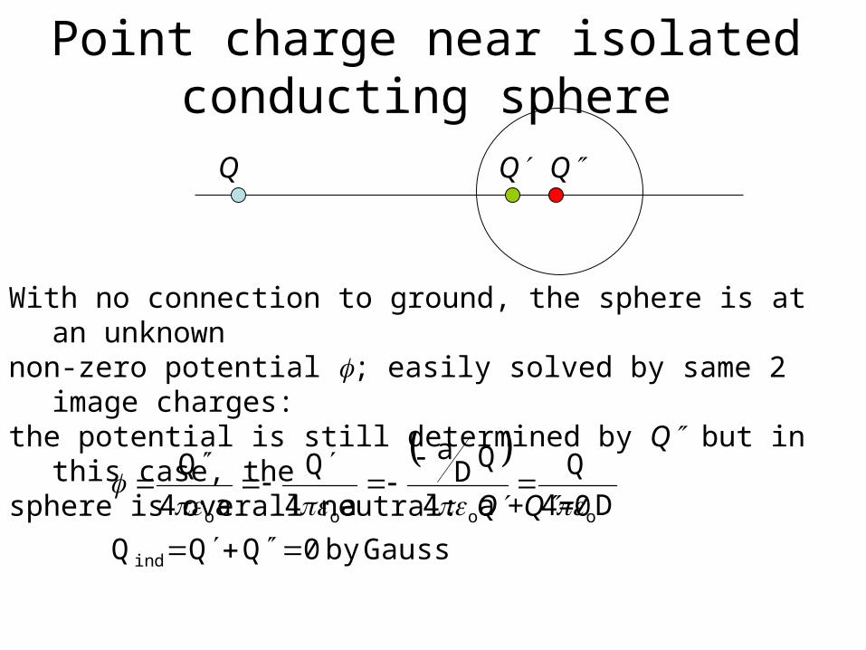
Point charge near isolated conducting sphere

With no connection to ground, the sphere is at an unknownnon-zero potential ; easily solved by same 2 image charges: the potential is still determined by Q but in this case, the sphere is overall neutral: Q+Q=0

(same potential as if sphere was absent!)

Gaussby 0QQ Q

D4

Q

a4

QDa

a4

Q

a4

Q

ind

oooo

Q Q Q

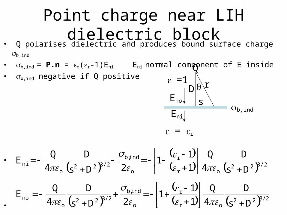
Point charge near LIH dielectric block• Q polarises dielectric and produces bound surface charge b,ind

• b,ind = P.n = o(r-1)Eni Eni normal component of E inside

• b,ind negative if Q positive

•

•

Q

Ds

r

Eni

Enob,ind

=1

= r

3/222

or

r

o

indb,3/222

oni

Ds

D

4

Q

1

11

2Ds

D

4

QE

3/222

or

r

o

indb,3/222

ono

Ds

D

4

Q

1

11

2Ds

D

4

QE

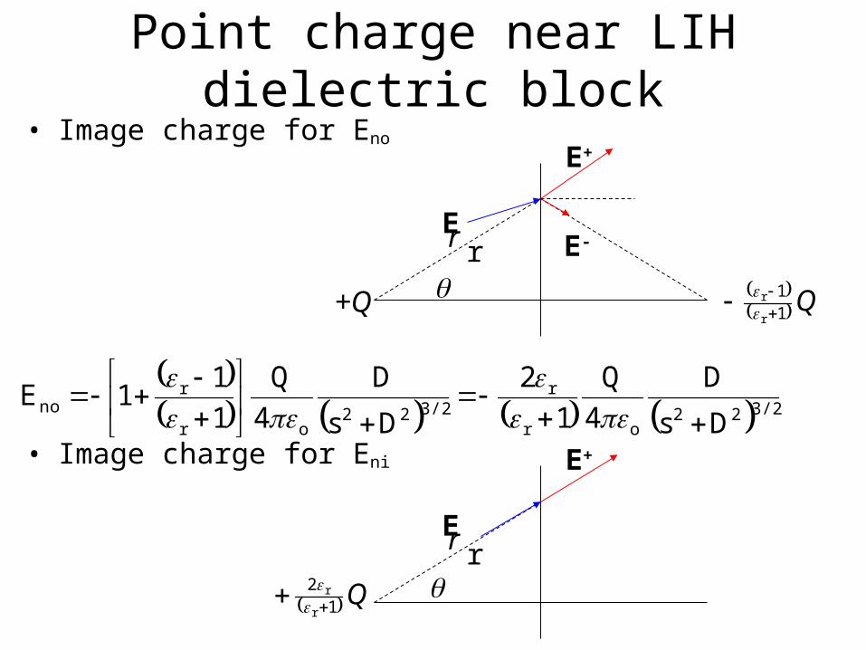
Point charge near LIH dielectric block• Image charge for Eno

• Image charge for Eni

+Q

rE

E+

E-

r

Q1

1

r

r

rE

E+

r

3/222

or

r3/222

or

rno

Ds

D

4

Q

1Ds

D

4

Q

1

11E

2

Q1r

r

2

Point charge near LIH dielectric block

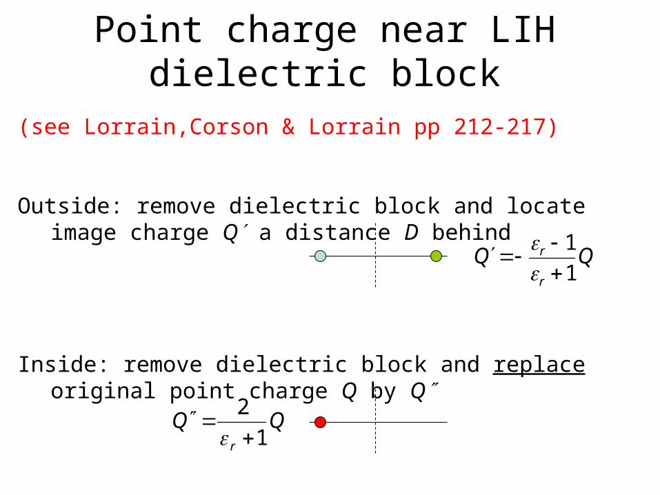
(see Lorrain,Corson & Lorrain pp 212-217)

Outside: remove dielectric block and locate image charge Q a distance D behind

Inside: remove dielectric block and replace original point charge Q by Q

Q r 1

r 1Q

QQr 1

2

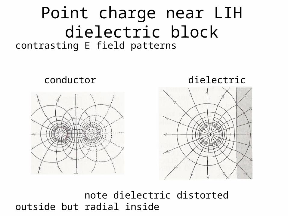
Point charge near LIH dielectric blockcontrasting E field patterns

conductor dielectric

note dielectric distorted outside but radial inside