methodology for the geochemical monitoring of an active ...

BRGM

methodology forthe geochemical monitoring

of an active volcanoin a dormant phase

Lamongan (East Java)

J.-C. BaubronExpert to the Volcanologicai Survey of Indonesia (Bandung)

with the collaboration ofJ.-C. Sabroux

Advisory VolcartologistB. Bourdon

assistantand MM. Yustinus Sulisto and Suryono

Merapi Volcanologicai Laboratory - Yogyakarta

September 198888 DT 035 ANA

BUREAU DE RECHERCHES GEOLOGIQUES ET MINIERESDIRECTION DE LA TECHNOLOGIE

Département AnalyseB.P. 6009 - 45060 ORLÉANS CEDEX 2 - France - Tél.: (33) 38.64.34.34

DIRECTORATE GENERAL OF GEOLOGY AND MINERAL RESOURCESGEOLOGICAL AND MINERAL SURVEY PROJECT - ADB.LN 641 INO

(Agreement n° 813/76/DDX 188}Volcanologicai Survey of Indonesia

Jalan Diponegoro 57 - BANDUNG 40122 INDONESIA

SUMMARY

Abstract

1 . Presentation

2. Method of surveillance

3. Monitoring instruments

4. Method of analysis

Pages

5 . Results

5.1. Traverses where no cracks

appeared in 02-1988

- Kenek-1

- West Ranu Pandan

5.2. Traverses close to the cracks

- Tjurah Buntu

- Gunung Kendeng

5

5

39

6. General interpretation

6.1. Flows of gas

6.2. Profiles

6.3. Concentrations

6.4. Thermal springs and mofettes

64

64

68

68

72

7. Conclusion

8. Recommendations

75

75

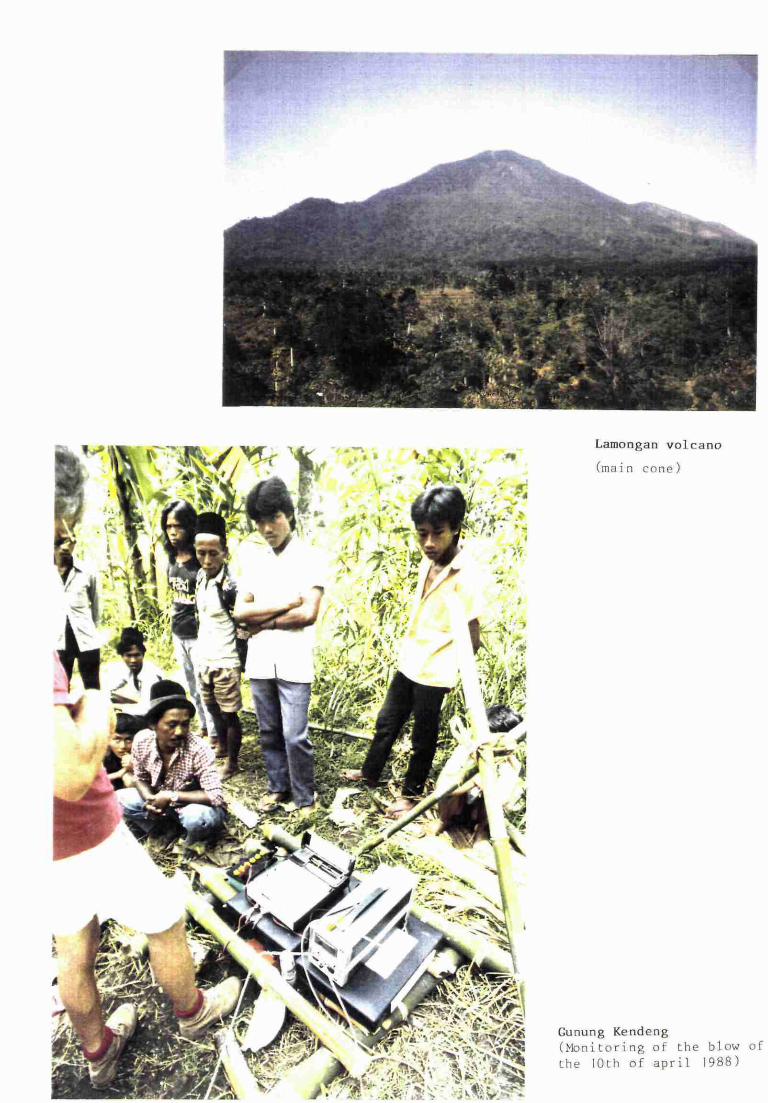
Lamongan volcano

(main cône)

Gunung Kendeng

(Monitoring of the blow of

the lOth of april 1988)

ABSTRACT

A three month geochernical survey of three components of

soil atmospheres (CO2, Rn, and He) carried out on the

western foot of the Lamongan volcano (E-Java) shows that the

thermal leak discovered six months before was still active.

The amount of gas escaping, now about 5 50 T per day of

CO2 from an area of 35 km^ , has increased strongly since

September 1987 and appears to be closely linked to the

seismicity. The February 1988 swarm is probably the cause of

the large increase observed.

The geochernical gas equilibrium leads to the conclusion

that the process involved is a hot water system expanding

upward into the upper crust. The remaining low levels of He.

suggest that the cause of this is more likely to be a deep

seismic event, rather than a dyke intrusion.

- 1 -

1. PRESENTATION

The Lamongan volcano, distinguished by the numerous

maars and eruptive vents located on its lower slopes,

presently in a dormant phase with only some low temperature

furaaroles in the summit crater, has been investigated for

its potential hazards in 1987 and 1988 (M. Aubert,

J.C. Baubron and D. Westercamp, 1988, Report in progress).

These results, obtained in September 1987, show that in

a large area located at the western foot of the main cone,

some of the anomalies observed give gas concentrations large

enough to indicate a regional thermal leak.

Most of the fissures of the 1978 and 1985 seismic

crisis were located in this zone. This target was also the

epicentre of the February 1988 swarm, which has focussed

attention on its present behaviour. For this purpose, the

surveillance of the cold outgassing through the ground

should be an effective method for estimating the volcanic

activity, locating the most active area, and possibly for

distinguishing the surficial effects (seasonal variations,

hot water movements near the surface) of the deep activity,

i.e. a magmatic intrusion into the upper crust.

2. METHOD OF SURVEILLANCE

Analyses have been made in four areas in the

surroundings of the site of the February 1988 crisis and at

the presumed limits of the affected area.

_ 1 _

The analyses were run once a month for 3 months on :

- Two areas previously investigated

. Where a narrow fault with an important gas leak

was revealed in September 1987. This is the

Kenek-1 traverse in the southern part of the

seismically active area where many cracks appeared

during the 1985 seismic swarm.

. In the northern part, across a recent roughly

NNW-SSE fault system of the volcano. This is the

W. RANÜ PANDAN traverse. No anomaly was observed

there in September 1987.

- Two areas where new cracks appeared during the crisis

of last February. These are namely the TJURAH-BUNTU

traverse, across a crack field, and the GUNüNG KENDENG

traverse, near the blow hole of the 10th April, 1988.

This type of surveillance is done using two kinds of

measurement :

. Concentrations of soil gases along traverses.

. Gas flow measurements on observed anomalies.

In addition, analyses of mofettes or gases from thermal

springs are compared with the previous work.

3. MONITORING INSTRUMENTS

Three components of the soil atmosphere are used;

carbon dioxide, radon and helium.

Why are these gases useful?

Carbon dioxide: Every thermal event in the crust will

induce degassing of the heated rocks, creating CO^ . For

instance, 0.5% of carbonates in the rocks over the area

affected by the heating, gives about 10® tonnes of CO2 for a

thickness of 10 km. Magmatic CO2 is not taken into account.

Radon: Radon is the direct daughter of radium and has

no intrinsic velocity. It is carried away by the underground

water, and there is a direct relationship between radon

activity and water temperature. As radon has a short

half-life (3.8 days), the investigations give information in

the range of about 100 metres below the surface.

Helium: This is the magmatic tracer. Helium is a

product of the uranium decay chain: every alpha particle

will give a helium atom. As it has the smallest atomic

radius of the rare gases, it has the highest intrinsic velocity

and it forms no compounds with other elements.

In practise, all the data published, and my own results

show that on an active volcanic field, the anomalous concen¬

trations of He fall in the range of 7 to 10 ppm or more (the

atmospheric concentration of helium is 5.2 ppm).

Thus, a gas survey based on these three components will

give information on three possible levels in the crust where

any magmatic intrusion would create distinctive anomalies:

- High activities of Rn will indicate a shallow thermal

anomaly, such as a hydrothermal convection cell.

- 4 -

Large CO2 concentrations, corrected for the surficial

biological contribution and related to a low Rn anomaly

will indicate a medium to deep thermal anomaly.

High concentrations of He (more than 7 ppm) will

indicate a deep thermal event.

4. METHOD OF ANALYSIS

- Sampling is done through a steel probe, 1 cm in diame¬

ter, with an internal teflon tube, driven into the soil

at a depth of 0.7 metres. The sampling interval is

usually 10 metres.

- Carbon dioxide is analysed with a field I.R. spectro¬

meter, so results are obtained on the spot, which can

be useful for choosing the next sampling point. In the

range 1% to 100%, the accuracy is typically 1%.

- Radon is analysed by alpha counting of ZnS-coated bulbs

filled with soil gas after elimination of the aerosols:

. First, on the spot in order to give an approximate

idea of the activity.

. Second, 3 hours later for accurate calculation of

the radon activity.

- Helium is analysed that evening, using a specific

mass-spectrometer after inflating a teflon bag of

0.5 litre of gas in the field.

_ =;

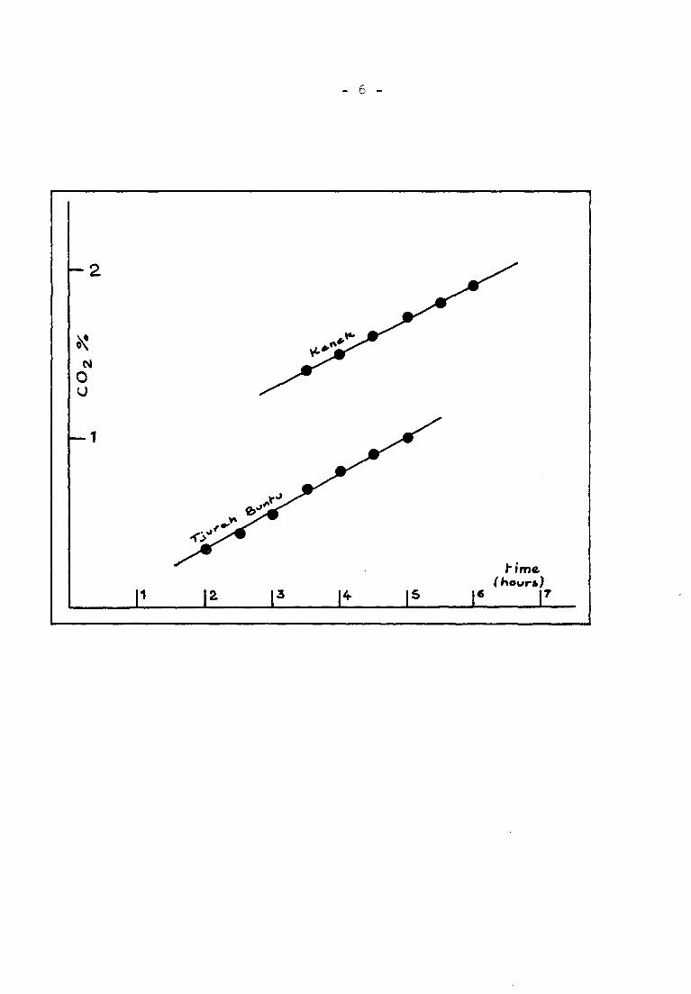
- Gas flow measurements are made in the following way:

. Half a container of about 150 1 and 0.6 m' is laid

down on a scraped area of ground, the open side

toward the soil .

. Gas samples are taken every half hour for 6 hours.

The graph of concentration against time usually gives a

straight line between T^, + 2 h and T^ + 6 h, which can be

taken as the mean increase per time unit. Flows are then

easily calculated.

5. RESULTS

5.1. Traverses where no cracks appeared in February

1968

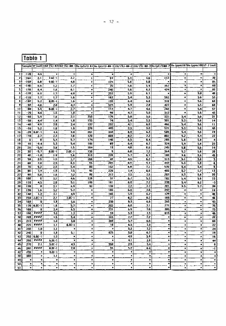
5.1.1. KENEK-1

This N-S traverse is located across the southern branch

of the track from Ranu Lamongan to Gunung An jar. The

negative sites are on the northern side, zero being at the

side of the track. It probably crosses a N 80 tectonic

direction active in 1985.

The trace of a fault found on this traverse in

September 1987 (Table 1 - Figure 1) was characterised by a

maximum CO^ concentration of 5% against a local background

of about 1%.

The general feature shows a continuous decrease of gas

concentrations from the anomaly to the limits of the

traverse, which can be explained as indicating a deep

convective cell, located near the zero point, whose effects

die away with distance from this point.

- 6 -

- 7 -

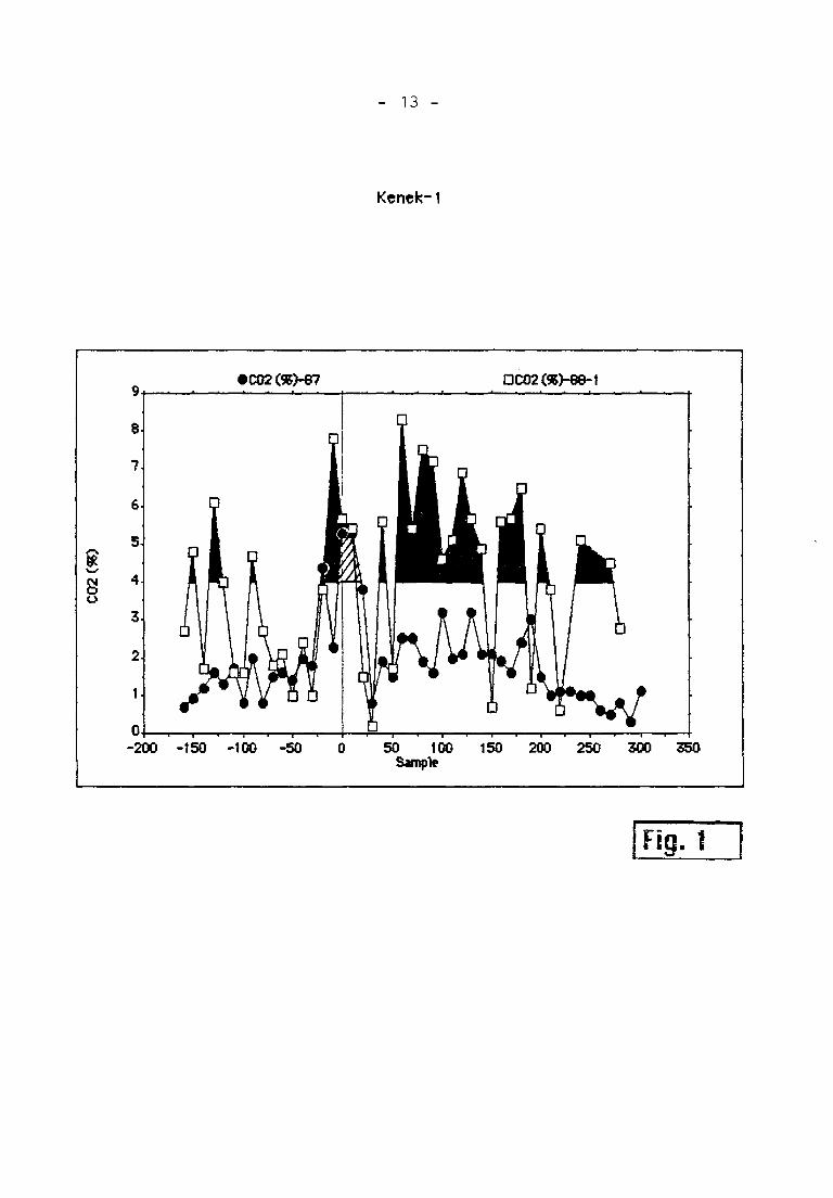
The self -potential measurements (SP) made in September

1987 (M. Aubert - Figure 2.1) show a slight decrease of

potential from north to south, with a small positive anomaly

(+ 50 mv ) near the 150-200 m sites.

This can be interpreted as a small convection cell in a

general groundwater transfer toward the north from the zero

point, in agreement with the topography.

We point out that the SP anomaly ends on its north side

where the sharp CO2 anomaly begins. This illustrates the

fact that the SP anomaly is located on the wetter soil where

the gas cannot exude because of lower permeability.

In March 1988 (Figure 2.2) the same SP traverse showed

a contrasting shape: the general elefctric signal is one

order of magnitude lower, with reduced noise; the trend to

the north is similar but there is a sharp negative anomaly

near the zero point, combined with a good positive anomaly

between the 50 and 100 sites.

The heavy rains explain the decrease of the electric

signal and the lower background, but the negative anomaly

associated with the positive anomaly is most probably

related to a convective cell in a fissure. This is probably

the 1987 system rejuvenated by the seismic swarm of February

1988.

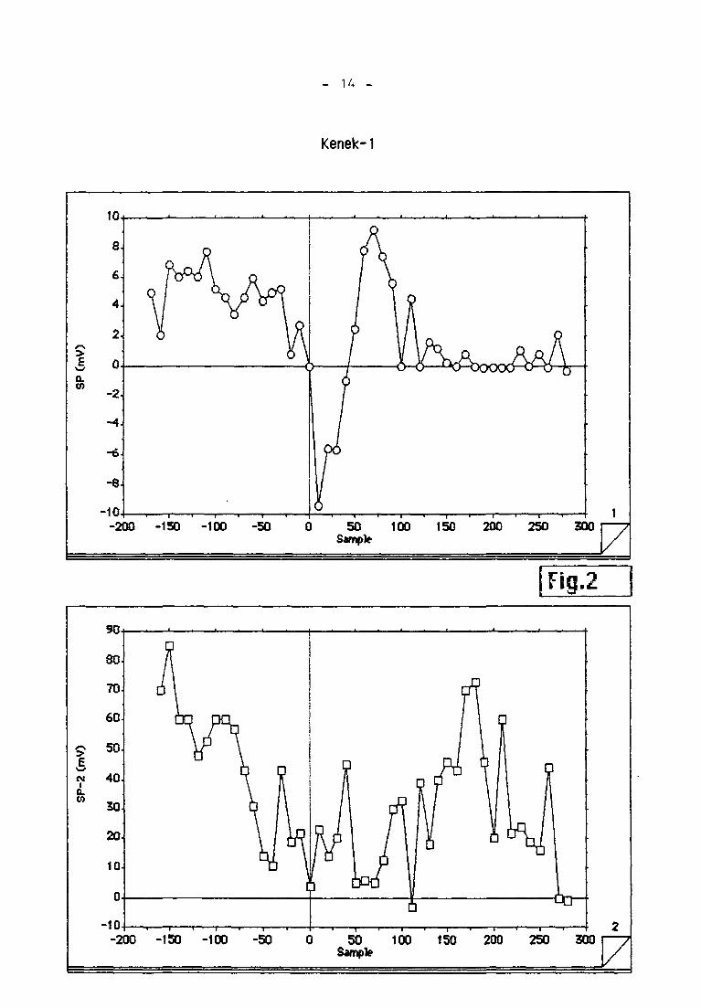
In March 1988 (Figures 1 and 3) the same traverse shows

a large increase of CO2 - traverse 88-1. In this figure, it

can be seen that the new profile is an homothetic

translation towards higher levels of CO2. The low values in

the first profile correspond to the lowest values in the new

one, in particular the negative anomalies near the "30" and

"-30" sites.

It should be noted that the highest increase is located

between the "50" and "200" sites, where the positive SP

anomaly was located in September 1987. Moreover, the highest

1988 concentrations of CO2 are linked with the positive

1988 SP anomaly.

It can be assumed that the convective cell found in

September 1987 is still operating and its intensity has

increased .

The same traverse, repeated once more in April (88-2,

Figure 3) shows that there has been a further increase.

While the highest values show a slight increase, the lowest

values display a large one.

The last measurements, made in May (88-3, Figure 4)

show the same increase again, but now there are almost no

samples with low levels. The highest CO2 value is strictly

connected with the positive SP anomaly.

It can be concluded that the surficial effect of the

deep thermal leak thus revealed continued for the three

months of survey. Soil CO2 measurements appear to be a good

instrument for appreciating the changes in the thermal

discharge from the ground, even when the absolute levels are

low (i.e. no apparent manifestation).

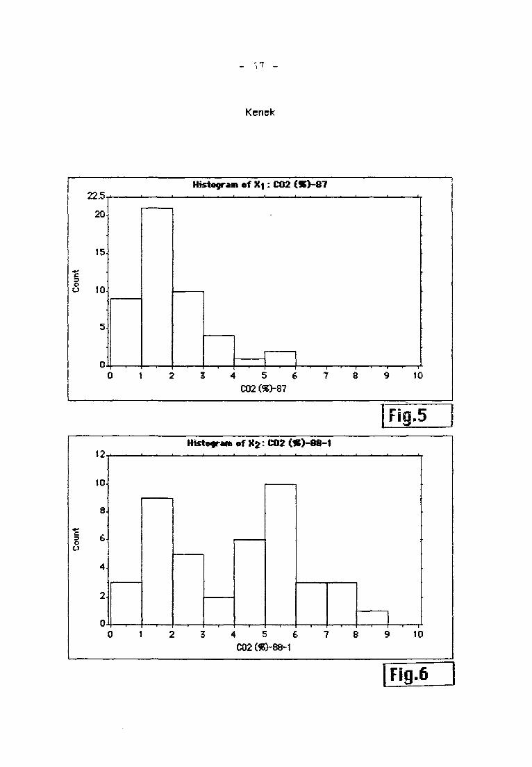
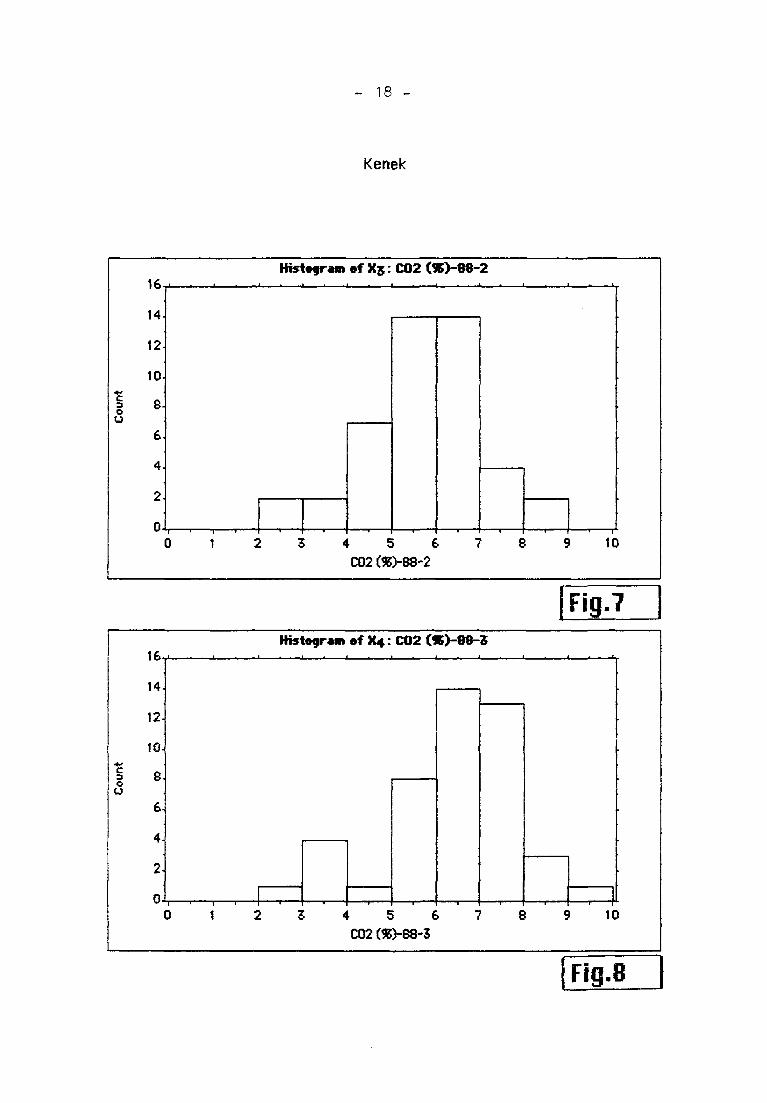
This phenomenon can also be observed with frequency

analysis, the mode increases regularly (Figures 5, 6, 7, 8).

- 9 -

The evolution of the histograms from 87 to 88-3 indi¬

cates that whereas the mode (45% of the data are between 1

and 2% cf CO2 ) was connected with the biogenic output in

September 1987, the distribution became bimcdal for the

first recording of 1988 : 22% of the samples remain between

1 and 2% of CO2 but 24% went up to 5 to 6%. The latter peak

is linked with the thermal leak.

The last two charts show the continuing increase: the

mode increases from the 5 to 7% CO2 level (60% of the

samples) to the 6 to 8% level in only a month.

This explains why the biogenic concentrations are in

the range of 1 to 2% and the surface effect of the thermal

leak about 4 to 5%. At the end of our experiments, most cf

the sites were within the thermal anomaly.

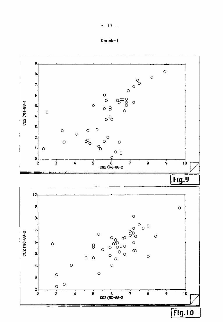
The close relationship between the successive

concentrations of CO2 is confirmed by the diagram where CO2

concentrations for the first month are plotted versus the

CO2 concentrations for the succeeding months (Figures 9

10). The correlation coefficients are respectively 0.82 and

0.74 for 88-1, 2 and 3.

As the result is a straight line, it can be concluded

that the increase of CO2 is proportional to the CO2

concentration. In this example, we have:

CO2 (t + 1) = CO2 (t) X 1.1

t = expressed in months.

CO2 = percentage of CO2

This implies that during a period of seismic activity

gas emanation increases exponentially with time. In this

case, dangerous levels (100% CO2 ) will be reached in less

than 2 years of seismic activity, from an initial background

level of about 3 to 4%.

- 10 -

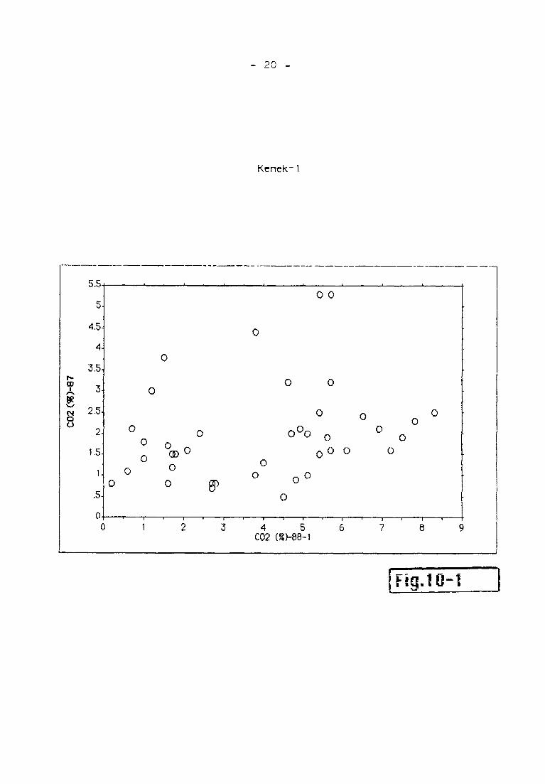
Data of September 1987 plotted against those of March

1988 show greater scatter (Figure 10-1): apart from the

September sites of high concentration, which have not moved

up, the sites of lowest concentration increase at the rate

of 1.6 a month, which is much higher than the rate measured

subsequently. But this was during the climax of the seismic

crisis .

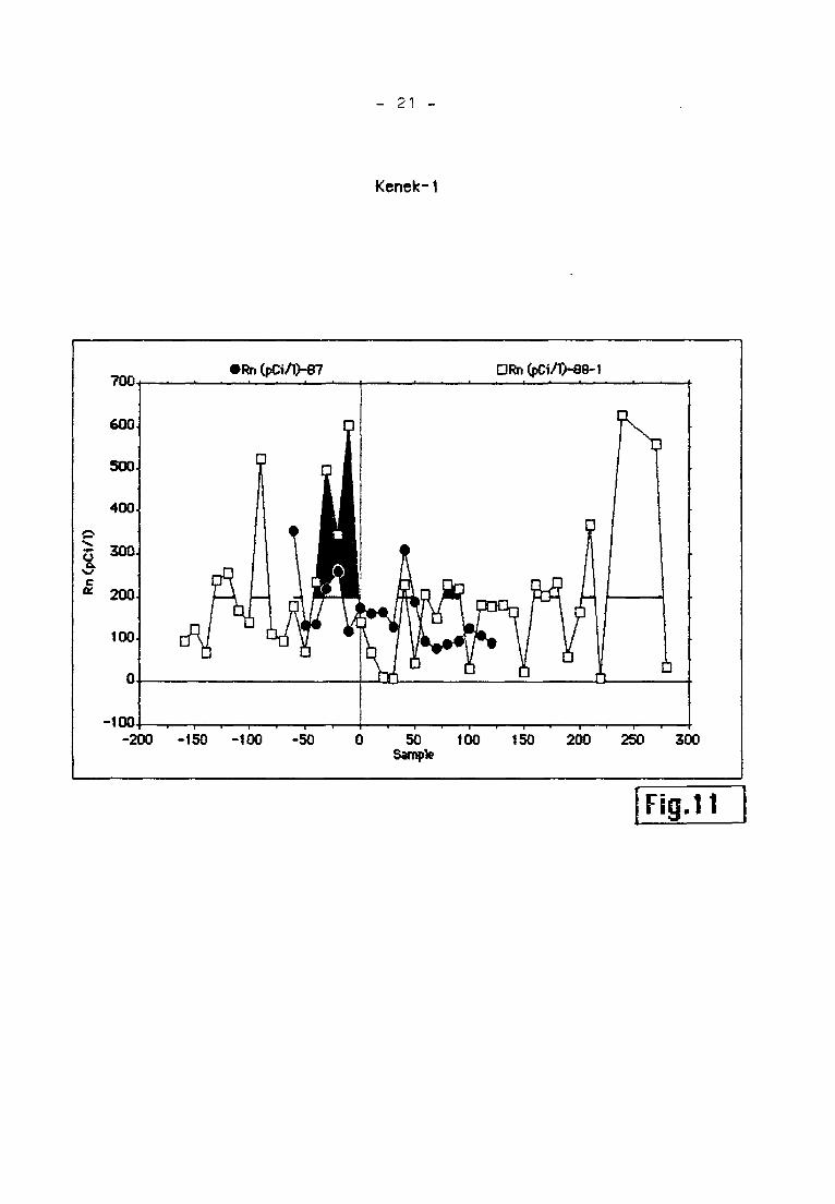
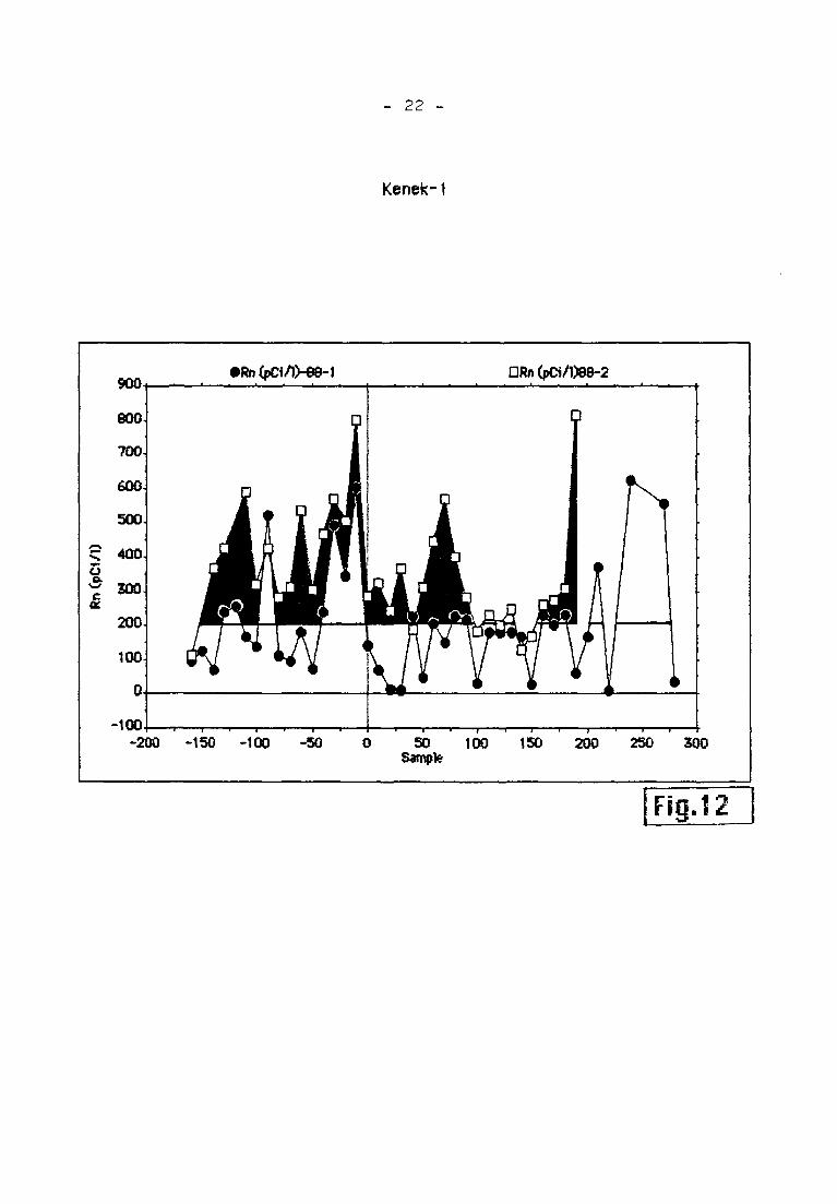
The radon spectrum shows the same relationship, the

main difference is that Rn maxima are on the edges of the

CO2 anomalies (Figures 11, 12). This was discernible in

September 1987 with the low activities but is much clearer

with the data obtained in March 1988.

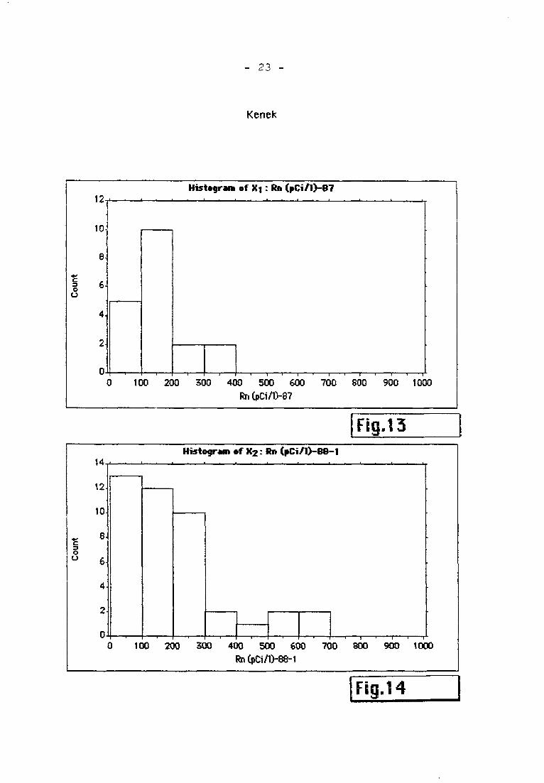
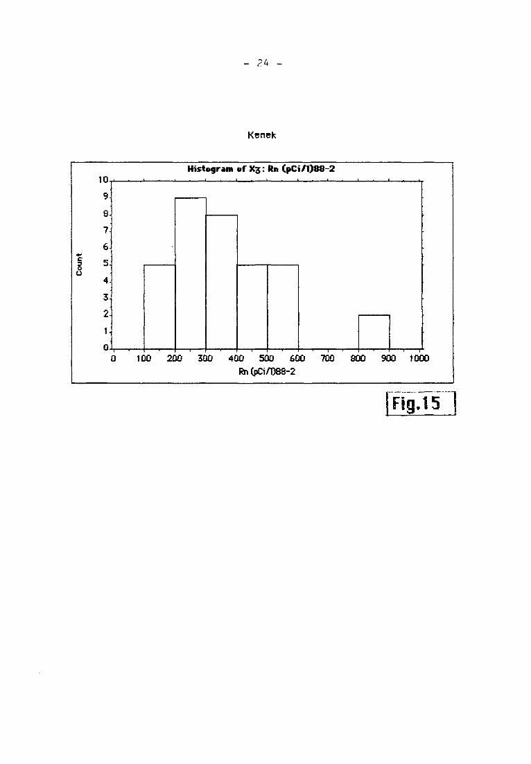
As for CO2, Rn activities rose to high levels: during

the investigations of 1988 I 600 to 800 pCi/litre. These

increases can be seen in the variation of the histograms,

most cf the samples have activities higher than

150 pCi/litre which is the common anomaly threshold (Figures

13, 14, 15).

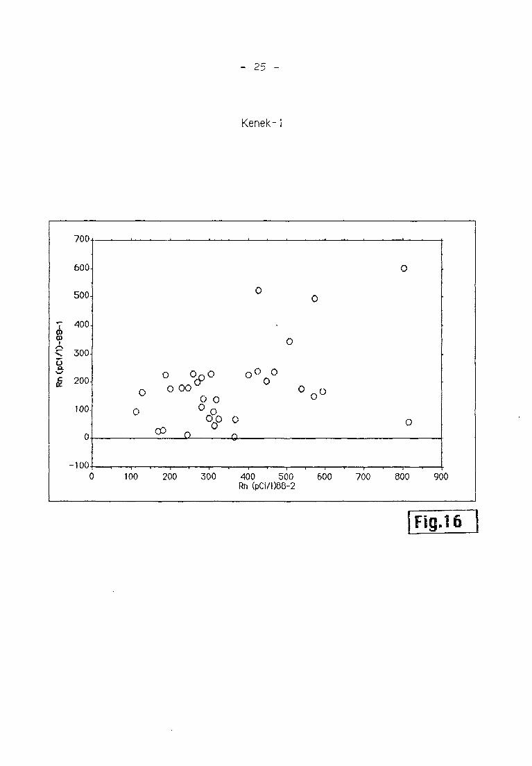
The diagram plotting the activities of radon, 88-1

versus 8S-2 (Figure 16) shows the increasing relationship,

which is in the form of:

Rn (T^ 1) = Rn ( T^ ) x 1.3

This is the same function as the relationship found

with the rises in CO2, i.e. an exponential increase cf Rn

activities with time.

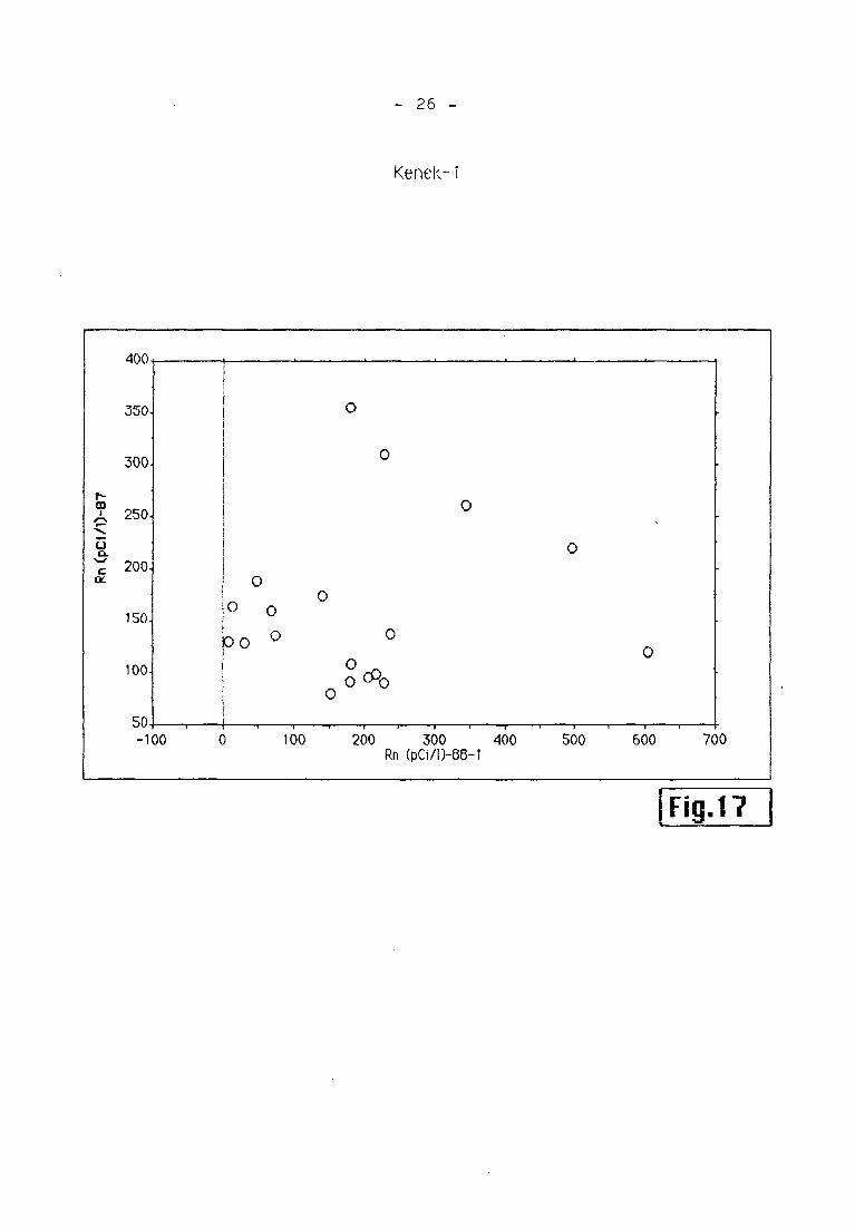
Data from the samples of last September 1987 plotted

against those of March 1988 (Figure 17) cannot be explained,

the seasonal changes in the climatic parameters probably

gave too many individual variations.

11 -

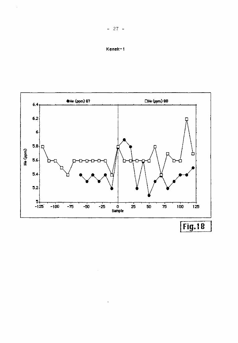
The He line chart (Figure 18) illustrates the point

that the levels are always in a low range, 0.2 ppm higher

than the results obtained in September 1987, but still

lacking any high concentration which would indicate a

magmatic component.

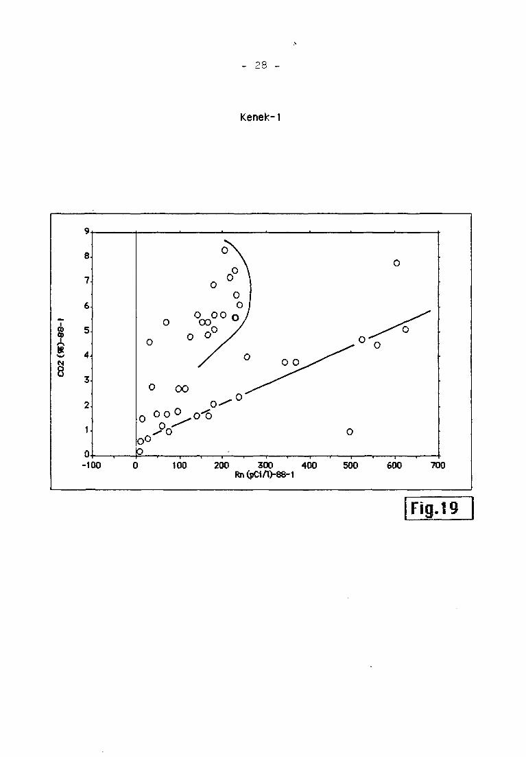
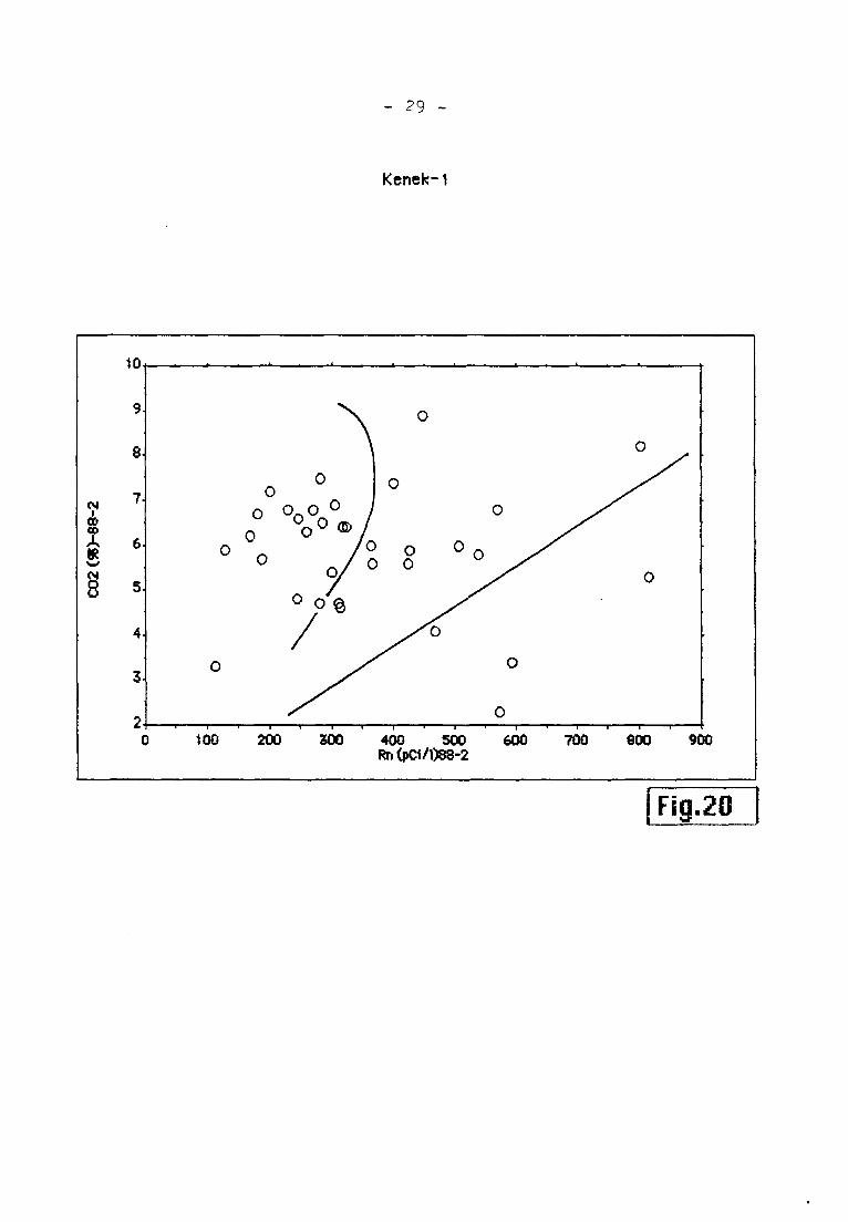
The diagrams plotting the CO2 concentrations versus Rn

activities show a two fold relationship (Figures 19, 20):

- The upper area (high CO2 relative to the medium Rn

values) corresponds to the highest He concentration of

the traverse.

- The lowest area (on a straight line) corresponds to

normal He.

With this kind of diagram, the places where the soil

atmosphere anomaly is produced by deep gases can be

distinguished from the samples where the gases are connected

with shallow ground water: this can be either originally

deep water from which the deep gases have previously been

extracted or rain water with a relative high horizontal

velocity (high radon) and/or an input of surficial

(biogenic) and deep CO2 after lateral transfer.

It can also reflect simply soil moisture: CO2 and He

escape more easily where the soil pores are not saturated

with water. In these sites, Rn activity is high because of

the direct relationship between Rn and water content. This

can explain the approximately inverse relationship between

He and Rn as shown on Figure 20.1.

The flow measurements show the same increase as seen in

the concentrations. The mean flow is about 0.4 l.m~^.h~^ of

CO2 (0.3 in April 22nd, 0.45 in May 6th).

12

Table 1

I

2

3

4

5

ft

7

a

9

IQ

II

12

13

)4

IS

16

17

18

19

20

21

22

23

24

2S

26

27

28

29

30

31

32

33

34

35

36

37

3B

39

40

41

42

43

44

45

4ft

47

40

49

50

51

Sttniple

-I/O

-160

-150

-140

130

-120

-no

-100

-90

-80

-70

-6U

-50

-40

-3D

-20

-10

0

10

20

30

40

50

60

70

80

100

MO

120

130

140

ISO

160

170

IBO

190

200

210

220

230

240

250

260

270

2H0

290

380

«

SP (iiiu)

4.9

2.1

6.0"

6.0

6.4

ft.O

7.7

5.2

4.6

3.5

4.6

5.9

4.4

4.9

5.2

B.OE-I

2.7

0

-9.4

-5.6

-5.7

-1.0

2.5

7.0

9.2

TA

5.6

0

L 4.5

0

1.6

1.2

2.0E-I

0

8.0E-t

0

####

1Ht»M

«###

#*#*

1.0

0

B.OE-t

####

2.1

«###

,

,

COZ CüJ-g?

B

^7.0E-I

9.or-ï

1.2

1.6

1.3

1.7

a.oE-i

2.0

B.OE-1

1.5

1.6

1.4

2.0

1.8

4.4

2.3

5.3

5.3

3.H

8.0E-I

1.9

1.5

2.5

2.5

1.9

" i'.ft

í:¿

2.0

3.1

3.2

2.1

2.1

1.9

1.6

2.4

3.0

1.5

1.0

t.I

1.1

1.0

1.0

6.0E-I

5.0c- 1

8.0F-1

3.0E-1

1.1

,

,

,

COZ(%)-Bi 1

2./

4.9'

1.7

6.1

4.0

1.6

1.6

4.7

2.7

1.0

2.1

1.0

2.4

1.0

3.0

7.8

5.7

5.4

1.5

2.0E-I

5.6

1.7

0.3

5.4

7.5

7.2

4.6

5.1

6.9

5.7

4.9

7.0E-1

5.6

5.7

6.5

1.2

5.4

3.8

6.0E-I

,

S.l

4.5

2.R

*

On (pCi/l)-fl7

1

355

135

137

220

261

120

174

160

164

130

.110

188

95

00

90

98'

12R

189

92

Hn (pCi/ll-HB-l

«

97

123

70

240

257

167

139

523

113

96

179

74

237

495

344

603

140

69

13

9

22B

47

205

152

228

2Í7"

31

toi

170

180

165

27

230

202

231

59

165

369

10

625

550

.tfi

,

,

,

,

C02 (%)-8H-2

3.3

5.6'

b.6

5.6

5.9

3.4

6.4

5.9

4.7

4.7

5.8

5.4

4.1

2.3

6.0

8.2

6.5

6.4

4.8

6.0

5.7

4.6

O.Q

6.8

_JA_

7.5"

6.7

6.0

7.2

6.6

5.9

6.2

6.3

6.8

6.9

5.3

7.2

5.7

6.5

5.3

5.0

4.9

4.1

2.5

5.2

a

«

«

C02 |%)-BB-3

3.0

5^0"

5.9

6.3

ft.1

5.3

6.0

2.8

4.6

5.0

5.U

5.5

6.0

3.0

6.3

7.2

8.4

6.7

8.0

7.2

6.7

6.2

9.7

7.1

^B.U

7.V

S.3

7.2

7.7

7.0

6.2

6.2

6.6

7.1

7.0

7.3

7.2

6.5

7-L

7.2

6.7

5.9

3.R

3.4

6.4

On (pCi/OBB-2

UÏ

u

ShI

424

592

318

427

282

312

53/

301

466

571

SOS

802

285

324

245

364

IBO

313

447

570

400

702

182

230

?ni

247

129

160

260

271

305

815

Ile (ppm) 87

5.4

5.3

5.4

5.3

5.4

5.2

5.8

5.9

5.8

5.2

5.6

5.1

5.3

5.4

5.2

5.3

5.4

5.4

5.5

-

He (ppm) 88

5.8

5.6

5.6

5.5

5.4

5.6

5.6

5.6

5.6

5.6

5.6

5.4

5.8

5.6

5.6

5.6

5.6

5.6

5.8

5.4

5.7

5.6

5.6

6.2

5.7

-n

SP-2 (mil)

7£

85

ftll

60

4H

53

60

60

57

43

3)

14

11

43

19

22

4

23

14

20

45

5

6

5

13^

~30

33

-3

39

IB

40

46

43

70

73

46

20

60

22

24

19

16

44

0

-1

m

*

- 13 -

Kenek- 1

9j

8.

7.

¿.

5.

4-

3

2

1

0

-200 -150

(%h&?

H

1 BH J

-100 -50 0 50 100

Sanóle

D(aï2(«)-e8-1

150 200 250 300 350

Fig. t

14 -

Kenek-1

>

£

CO

10-r

8.

£.

4.

2.

0.

-2.

-4.

-6-

-8

-10.

-200 -150 -100 -50 C) 50

Sample

100

1

150 200 250

1

300

/

Fig.2

>

E

ot

I

0.

CO

15 -

Kenek-1

CD

>1

ta

C02

IOh

9.

8.

7.

6.

5.

4

3.

Is)1.

0

-2(

(«)-88-1

DO -150 -100 -50 £

DC02 (SÇ)-e8-2

) 50

SaiT^>1e

100 150 200 250 300

ng. 5

- 16 -

Kenek- 1

ZOO

IOh

9

8

7.

6

5.

4

3.

2.

(«>88-2

-20) -150 -100 -50 £

DC02 («)-8e-3

) 50

Sample

too 150 200 250 300

Fig.4

- 17 -

Kenek

Hist«9rmi of Xi : C02 (fS)-87

22 5,

20.

15.

c

O

a 10.

5.

0.

j

1

012345678

C02 (S5)-87

9 10

Fig.5

12,

10

8.

1 'o

4.

2.

0.

Histo^TMii X2: C02 (fK)-88-1

[) 1 2 3 4t 5 6 7 8 9 IC

C02 («)-88-1

>

Fig.6 1

18 -

Kenek

Count

Histeçram «f X3: C02 («)-88-2

14

12

10.

8-

6.

4.

2

0.

01 23456789 10

C02 («)-88-2

Fíg.7

c

s

o

o

16

14

12.

10

8

6.

4

2.

n.

HistogrAin of X4: C02 («)-88-3

T1111

4 5 6 7

C02 («)-88-3

9 10

Fig.8

- 19 -

Kenek- 1

1

8

a»1

3

9

8.

7

6

5

4.

3

2.

1.

0

^

0

o

0

0

0

1 1 1 1

i 3 4

00

0

o

0

'-^ 4) 0 00-0

0 9 0

o 0

o

CPQ 0 0

o 0

o1 1 1 '

5 6 7

C02 («)-88-2

0

1

8

o

9 10

/

1 Fig.9

CM1

ODOD

A

g

CM

O

u

IOj

9.

8.

7

6

5.

4.

3

0

f

0

o

0

0 ^

i 3 4

0

o

0 0

8 , o°?oo °

o 0 "" 0

O

O

5 6 7

C02(«)-88-3

0

0

0

8

0

9 10

/

ÍFlg.lQ

- 20 -

Kenek- 1

1^

001

^"W/

002

55

5-

4.5

4-

3.5.

3.

2.b.

2.

1.5.

1.

.b.

0.

0

0

O

0

o

0

0

1

0

0

0 o

O

0 ^

1 1

2 3

0 0

0

0 0

On 0^ 0

^ ^ 0 O

QUO 0

0

0 ^0o

0

1 . 1 . 1 . I r r T

4 5 6 7 8 ç

C02 (?.)-88-1

)

Fig.io-i

- 21 -

Kenek-1

700 J

600

St».

400

1 300.a.

c

"^ 200.

100.

0.

-100.

-2(

(pCi/l)-e7

30 -150 -100 -50 C

DRn (pCi/l)-88-1

1

' 1

i

I 50

Sample

100 150 200 250 300

Fig.11

- 22

Kenek- 1

9(»H

800

7tK).

600.

500

s *°°u

(pCi/1)-^-1 DRn (fCiñ)eB-2

200

100.

0.

-100.' I1 I I Ir- -I111- -I11-

-200 -150 -103 -50 0 50 100 150 200 250 300

Sample

Fig. 12

- 23 -

Kenek

Count

Hisioçrom of Xl : Rn (pCi/1)-87

10.

8.

6.

4.

2.

01 1 11111111prr'

0 100 200 300 400 500 600 700 800 900 1000

Rn (pCi/1)-87

Fig.î3

Count14,

12-

10.

8

6

4.

2

n.

Histoçrom of X2: Rn (pCi/1)-88 -1

11111r"-

100 200 300 400 500 600 700 800 90> 1000

Rn (pCi/l)-88-1

Fig.14

- 24 -

Kenek

Count

10,

9.

8

7.

6

5.

4.

3.

2.

1.

0.

0 100

Histogram of X3: Rn (pCi/1)88-2

200 300 400 500 600 70)

Rn (pCi/l)88-2

&X)

,

900 1000

Fig.l 5 1

- 25 -

Kenek-

700

-89-1Oo.-^

c

0¿

600

500

400

300

200

100

-100

0

o

oo 00

oô qO o

o

03

o o

op O

%^

J2_

o

O 100 200 300 400 500 600 700 800 900

Rn (pCi/l)88-2

Fig.l 6

26 -

Kenek-

81

uCL

C

OL

350.

300.

2.50.

200.

150.

100-

50.

0

û 0

OO °

1,i,r

o

0

0

0

o cô0

11 1

0

-111

0

>1 1

.

0

'

1!

-100 0 100 200 300 400 500 600 700

Rn (pCi/l)-88-1

Fig.l 7

- 27

Kenek-1

6 4i

62

6

5.8

1f 5.6z

5.4.

5.2

5

-125 -IM

(ppm) 87

-75 -50 -25 0

Sw^le

25

DHe (ppm) 88

50 75 1(H3 125

Fig.18

- 28 -

Kenek- 1

Fig.l9

104

- 29 -

Kenek- 1

CM)

OD

OD

A

cs

8

9.

8

7-

6

5.

4

3.

O

0

00

0° \°°Vo/° 0

0 /o 0

0 o4o

o

I Ir- -I11 111r-

100 200 300 400 5CN3 600

Rn (pC1/i:e8-2

700 800 9CH3

Fig.20

iO -

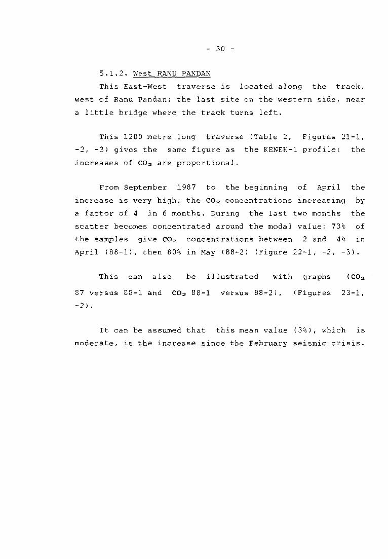
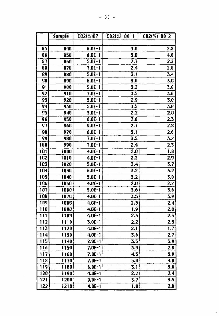
5.1.2. West RANU PANDAN

This East-West traverse is located along the track,

west of Ranu Pandan; the last site on the western side, near

a little bridge where the track turns left.

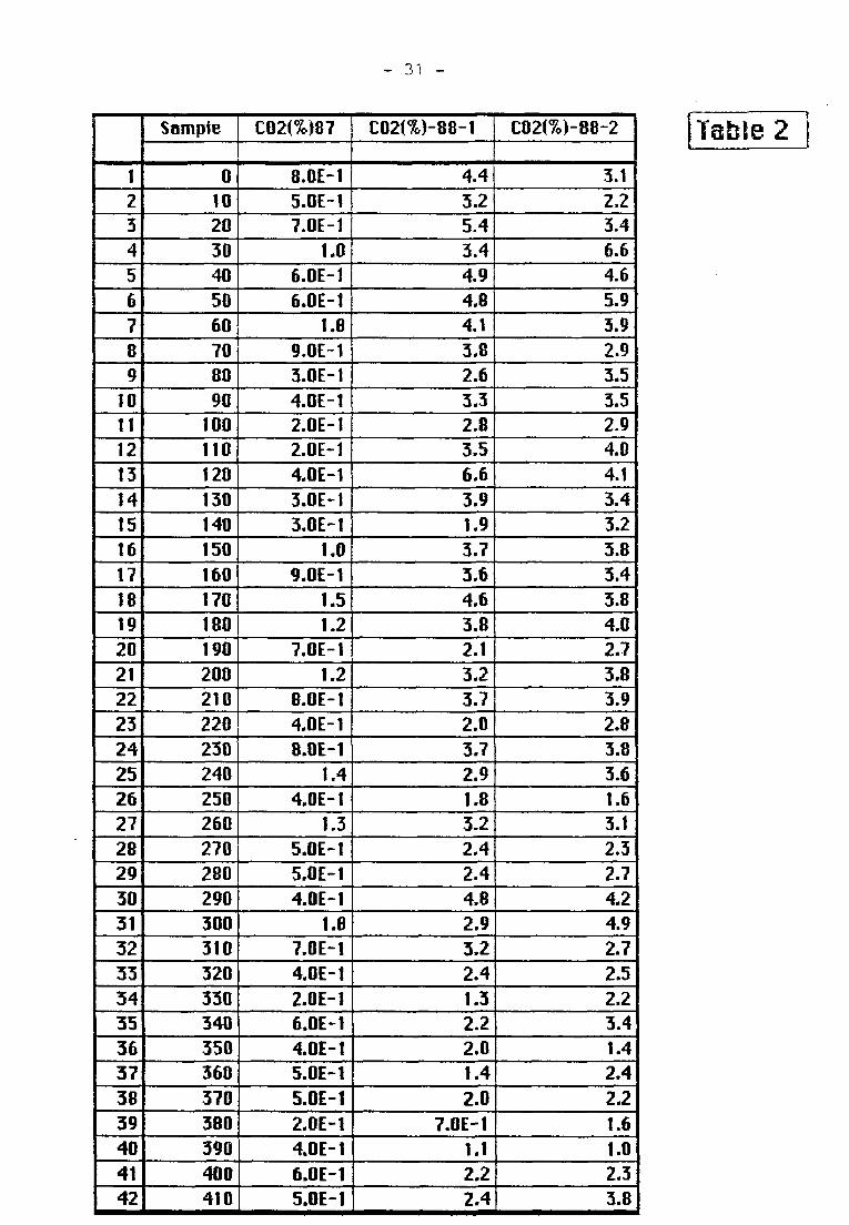
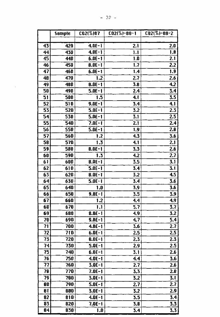
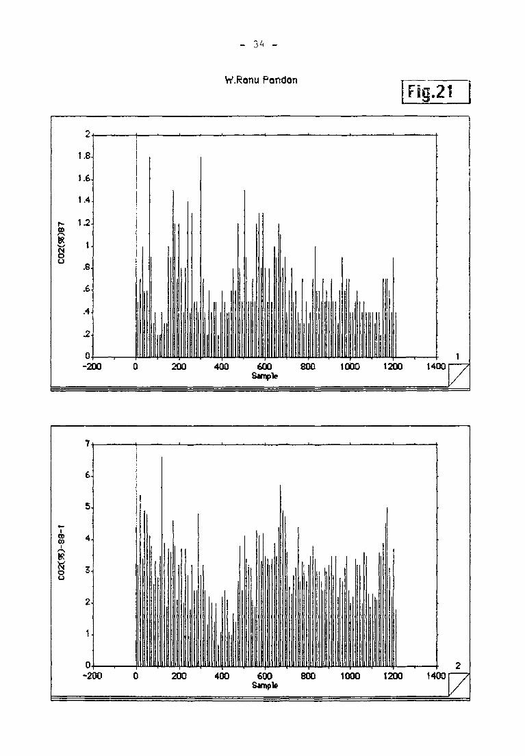
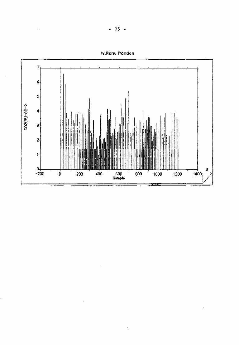
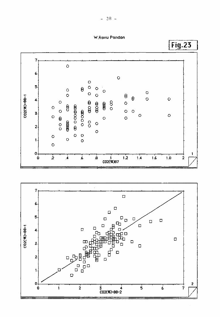
This 1200 metre long traverse (Table 2, Figures 21-1,

-2, -3) gives the same figure as the KENEK-1 profile: the

increases of CO2 are proportional.

From September 1987 to the beginning of April the

increase is very high; the CO2 concentrations increasing by

a factor of 4 in 6 months. During the last two months the

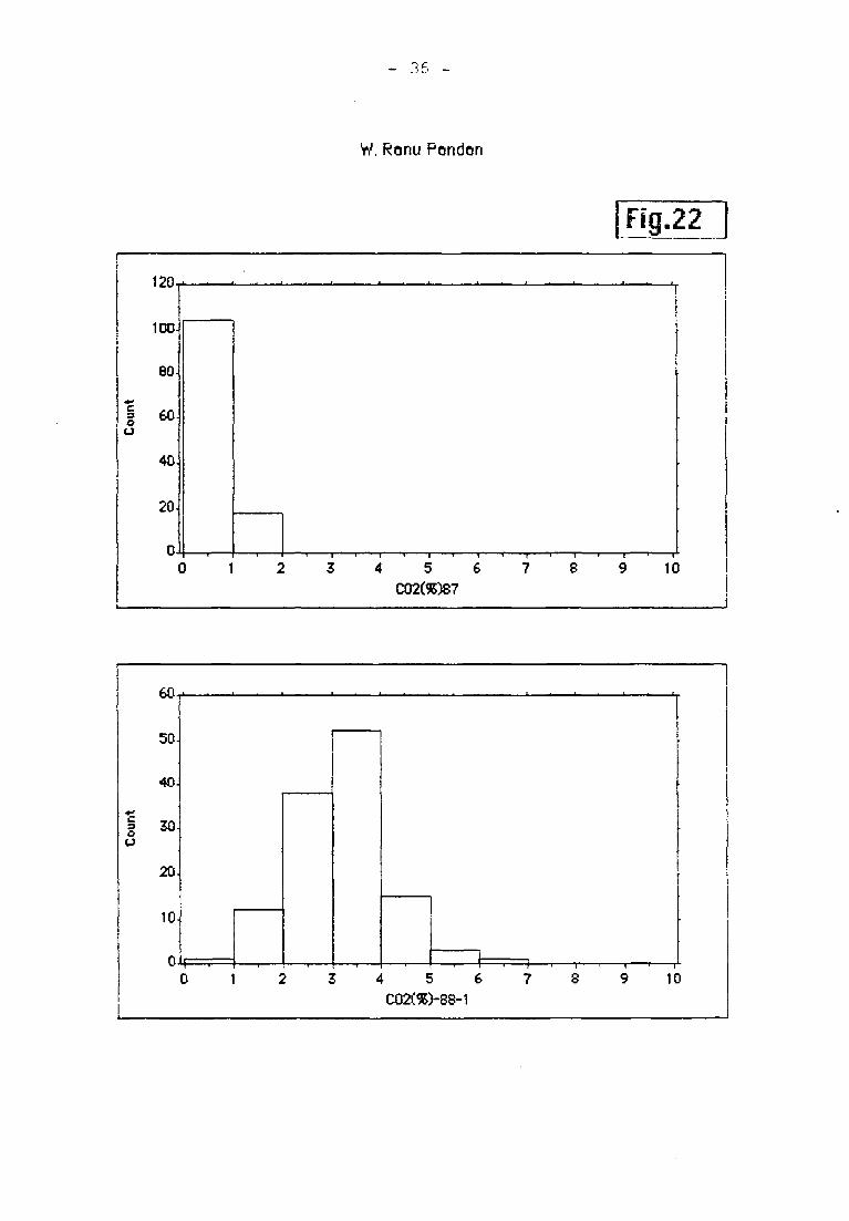
scatter becomes concentrated around the modal value: 73% of

the samples give CO2 concentrations between 2 and 4% in

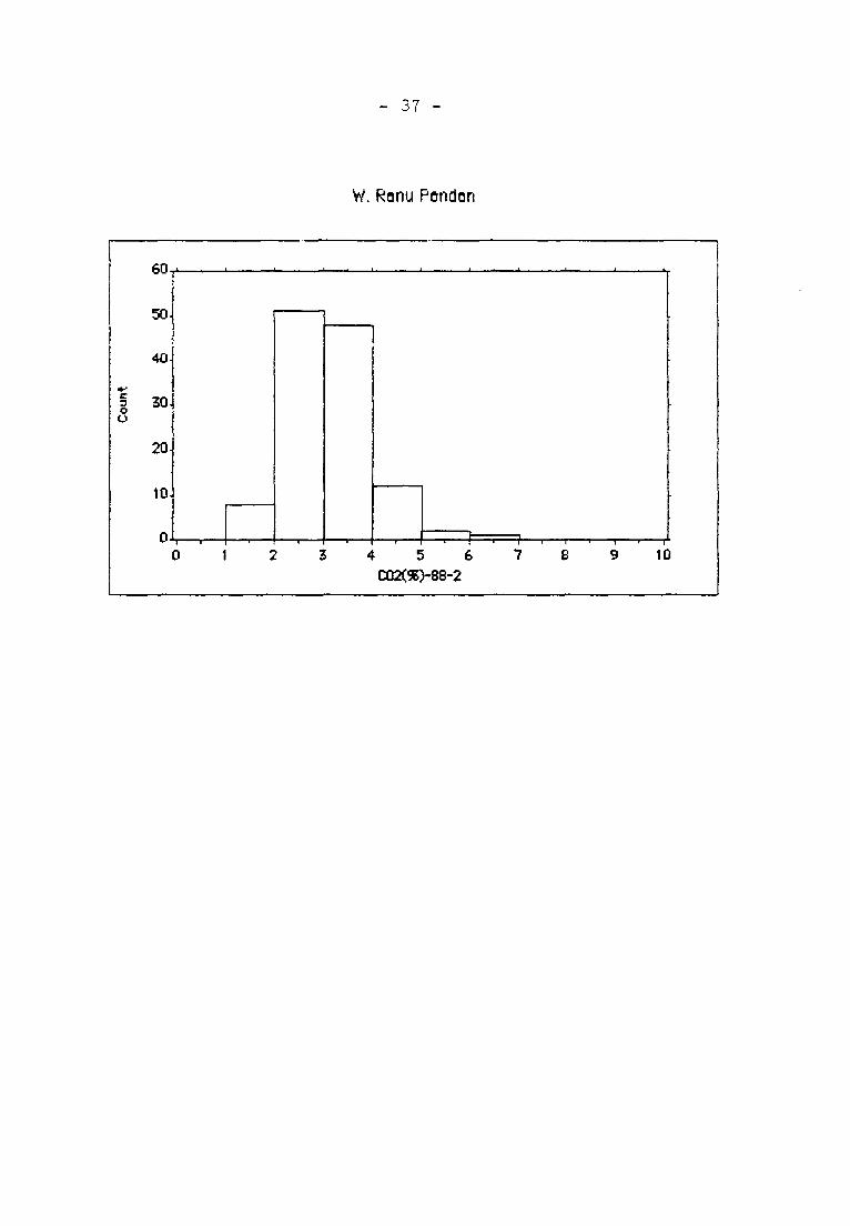
April (88-1), then 80% in May (88-2) (Figure 22-1, -2, -3).

This can also be illustrated with graphs ( CO2

87 versus 88-1 and CO2 88-1 versus 88-2), (Figures 23-1,

-2) .

It can be assumed that this mean value (3%), which is

moderate, is the increase since the February seismic crisis.

- 31 -

1

2

3

4

5

6

7

8

9

10

11

12

13

14

15

16

17

18

19

20

21

22

23

24

25

26

27

28

29

30

31

32

33

34

35

36

37

38

39

40

41

42

Sample

0

10

20

30

40

50

60

70

80

90

100

110

120

130

140

150

160

170

180

190

200

210

220

230

240

250

260

270

280

290

300

310

320

330

340

350

360

370

380

390

400

410

C02(%)87

8.0E-1

5.0E-1

7.0E-1

1.0

6.0E-1

6.0E-1

1.8

9.0E-1

3.0E-1

4.0E-1

2.ÜE-1

2.0E-1

4.0E-1

3.0E-1

3.0E-1

1.0

9.0E-1

1.5

1.2

7.0E-1

1.2

8.0E-1

4.0E-1

8.0E-1

1.4

4.0E-1

1.3

5.0E-1

5.0E-1

4.0E-1

1.8

7.ÜE-1

4.0E-1

2.0E-1

6.0E-1

4.DE-1

5.0E-1

5.0E-1

2.0E-1

4.0E-1

6.0E-1

5.0E-1

C02(%)-88-l

4.4

3.2

5.4

3.4

4.9

4.8

4.1

3.8

2.6

3.3

2.8

3.5

6.6

3.9

1.9

3.7

3.6

4.6

3.8

2.1

3.2

3.7

2.0

3.7

2.9

1.8

3.2

2.4

2.4

4.8

2.9

3.2

2.4

1.3

2.2

2.0

1.4

2.0

7.ÜE-1

1.1

2.2

2.4

C02(%)-88-2

3.1

2.2

3.4

6.6

4.6

5.9

3.9

2.9

3.5

3.5

2.9

4.0

4.1

3.4

3.2

3.8

3.4

3.8

4.0

2.7

3.8

3.9

2.8

3.8

3.6

1.6

3.1

2.3

2.7

4.2

4.9

2.7

2.5

2.2

3.4

1.4

2.4

2.2

1.6

1.0

2.3

3.8

¡Tablez

- 32

43

44

45

46

47

48

49

50

51

52

53

54

55

56

57

58

59

60

61

62

63

64

65

66

67

68

69

70

71

72

73

74

75

76

77

78

79

80

81

82

83

84

Sample

420

430

440

450

460

470

480

490

500

510

520

530

540

550

560

570

580

590

600

610

620

630

640

650

660

670

680

690

700

710

720

730

740

750

760

770

780

790

800

810

820

830

C02(%)87

4.0E-1

4.0E-1

6.0E-1

8.0E-1

6.0E-1

1.2

8.0E-1

5.0E-1

1.5

9.0E-1

5.0E-1

5.0E-1

7.0E-1

5.0E-1

1.2

1.3

8.0E-1

1.3

8.0E-1

5.0E-1

8.0E-1

5.0E-1

1.0

9.0E-1

1.2

1.1

8.0E-1

9.0E-1

4.0E-1

6.0E-1

8.0E-1

5.0E-1

6.QE-1

4.0E-1

3.0E-1

7.0E-1

3.0E-1

5.0E-1

3.0E-1

4.QE-1

7.0E-1

1.0

C02(%)-88-l

2.1

\.\

1.0

1.7

1.4

2.7

3.8

2.4

4.1

3.4

3.2

3.1

2.1

1.9

4.3

4.1

3.3

4.2

3.5

3.4

3.2

3.4

3.9

3.5

4.4

5.7

4.9

4.7

3.6

2.5

2.3

2.9

3.1

4.4

2.7

3.3

3.2

2.7

3.2

3.5

3.8

3.4

C02(%)-88-2

2.0

1.8

2.1

2.2

1.9

2.6

4.2

3.4

3.5

4.1

2.3

2.5

2.4

2.8

3.6

2.1

2.6

2.7

3.1

3.1

4.5

3.6

3.6

3.9

4.9

3.7

3.2

5.4

2.7

2.5

2.3

2.5

2.6

3.6

2.6

2.8

3.1

2.7

2.9

3.4

3.3

3.3

33 -

85

86

87

88

89

90

91

92

93

94

95

96

97

98

99

100

101

102

103

104

105

106

107

108

109

110

111

112

113

114

115

116

117

118

119

120

121

122

Sample

840

850

860

870

880

890

900

910

920

930

940

950

960

970

980

990

1000

1010

1020

1030

1040

1050

1060

1070

1080

1090

1100

1110

1120

1130

1140

1150

1160

1170

1180

1190

1200

1210

C02(%)87

6.0E-1

6.0E-1

5.0E-1

7.0E-1

5.0E-1

6.0E-1

5.0E-1

7.0E-1

5.0E-1

5.0E-1

3.0E-1

6.0E-1

9.0E-1

6.0E-1

7.0E-1

7.0E-1

4.0E-1

4.0E-1

5.0E-1

6.0E-1

5.0E-1

4.0E-1

5.0E-1

4.0E-1

4.0E-1

4.0E-1

4.0E-1

3.0E-1

4.0E-1

4.0E-1

2.0E-1

7.0E-1

7.0E-1

7.0E-1

6.0E-1

4.0E-1

9.0E-1

4.ÜE-1

C02(%)-88-l

3.0

3.0

2.7

2.4

3.1

3.0

3.2

3.5

2.9

3.5

2.2

2.8

2.7

3.1

3.5

2.4

2.0

2.2

3.4

3.2

3.2

2.0

3.6

3.5

2.3

1.9

2-3

2.2

2.1

3.6

3.5

3.9

4.5

5.0

3.1

2.2

3.7

1.8

C02(%)-88-2

2.8

4.0

2.2

2.8

3.4

3.0

3.6

3.6

3.0

3.0

2.0

2.3

2.8

2.6

3.2

2.3

1.8

2.9

3.7

3.2

3.0

2.2

3.6

3.9

2.4

2.0

2.3

2.3

1.7

2.7

3.9

2.8

3.9

4.0

3.6

2.4

3.5

2.8

- 3A -

W.Ronu Pondon

Fig.21

r^

00

Su

2^

1.8.

1.6.

1.4

1.2.

1

.8.

.6.

.4.

2.

0.

-2tM3 200 400 600 8tK) 1000 12ÍXI 1400

Sample

- 35 -

W.Ranu Pandan

- 36 -

W. Ronu Pondon

Fíg.22

120,

100.

80

1 60.u

40.

20.

0.u.* 1 I

0 1 2

1 1

3

1 I 1 1

4 5 6

C02(SC)87

7 8

1

9

' 1

10

- 37 -

W. Ronu Pondon

Counf

£rO ,' >^^L, ^111.

50

40.

30

20.

10

û 1

0 12 3 4 5 6

C02CSÇ)-88-2

1(

7

1r^'

8

11

9

'

10

- 38 -

W.Ronu Pondon

Flg.25

I

o»

8

CM

O

CJ

£ 1 12

C02(%)87

I

OD

o

u

3 4

C02(9K>88-2

5.2. Traverses close to the cracks

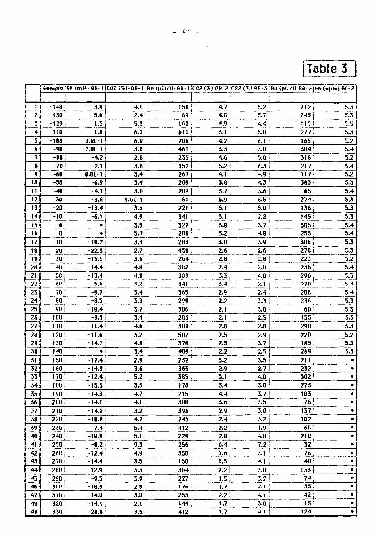
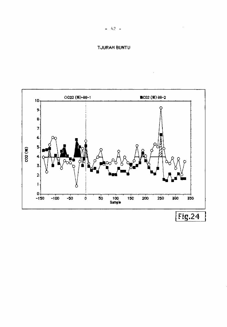
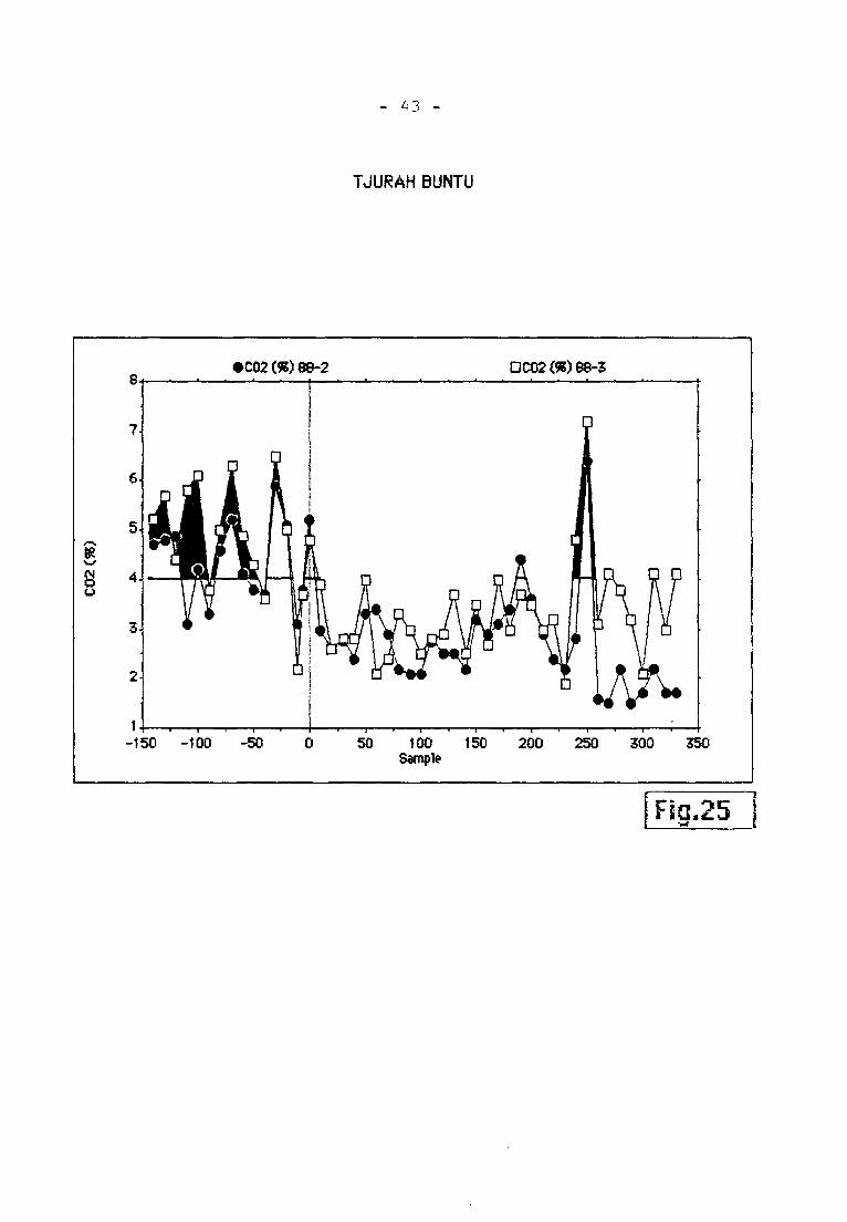
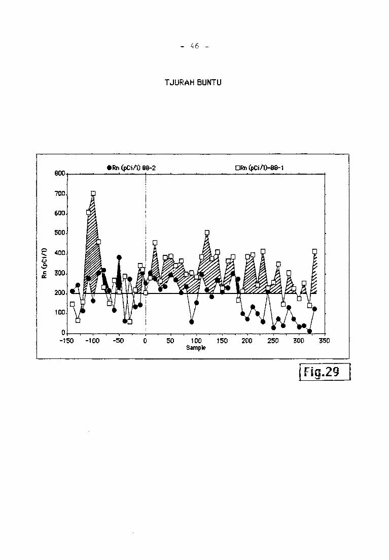
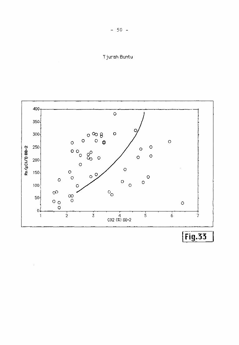
5.2.1. TJURAH BUNTU

This N-S traverse crosses the cracks of last February.

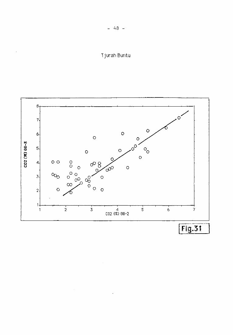
Measurements were made along it three times (Table 3,

Figures 24, 25). Once again the relationships are the same,

but here, although the level was high in March (88-1), a

slight decrease occured in April (88-2), and a small

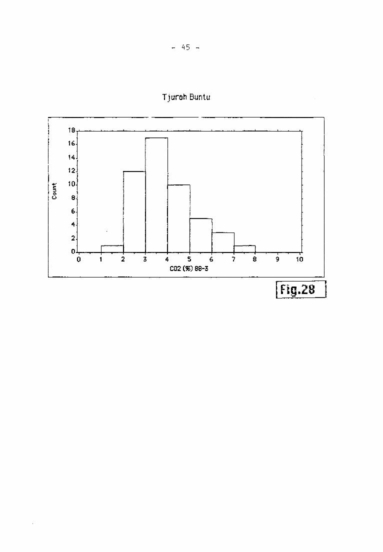
increase at the beginning of May (88-3). This can also be

seen in the frequency analysis (bar graphs.

Figures 26, 27, 28), where 49% of the samples were in the 3

to 4% space the first month, 37% in the 2 to 3% space the

second month and 35% in the 3 to 4% space again in the last

month .

In detail, the northern side of the traverse (negative

sites) shows a permanent increase. It should be noted that

the part of the traverse where the cracks occurred is the

part with the mean lowest CO2 concentrations and where the

instability is most apparent. Reaction with the open cracks

is possible.

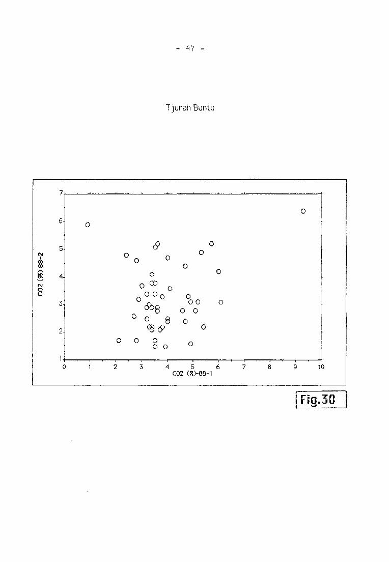
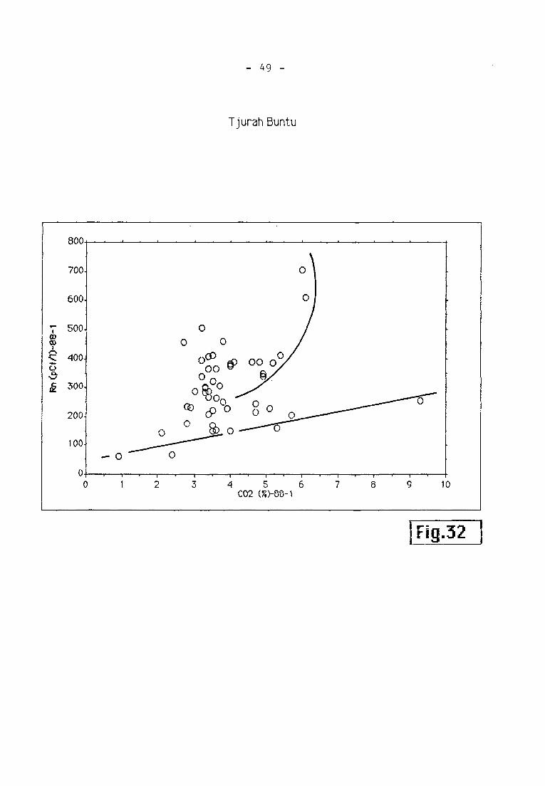
As before, Rn activities are connected with CO2 concen¬

trations. Rn frequency diagrams show the same decrease

between 88-1 and 88-2 as that displayed by CO2 (Figures 29,

30, 31, 32, 33).

However the highest Rn activities are found in the

sites where the low concentrations of CO2 are low. Moreover,

near site -100, the CO2 concentration increases as the Rn

activity decreases.

He is always quite low: 5.4 to 5.5 ppm only.

- 40 -

COa flows vary from 0.5 in the first month tc 0.3 then

to 0.4 in the last month (expressed as litres per hour per

square metre). The place where the measurements were made is

located near the -100 m site.

In this traverse, the depressed zones correspond to the

areas where the cracks are located. This has also been

observed at a smaller scale. The cracks are open systems

connected with the free atmosphere where the atmospheric

component is the most important in the gas mixture.

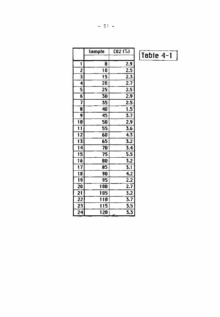
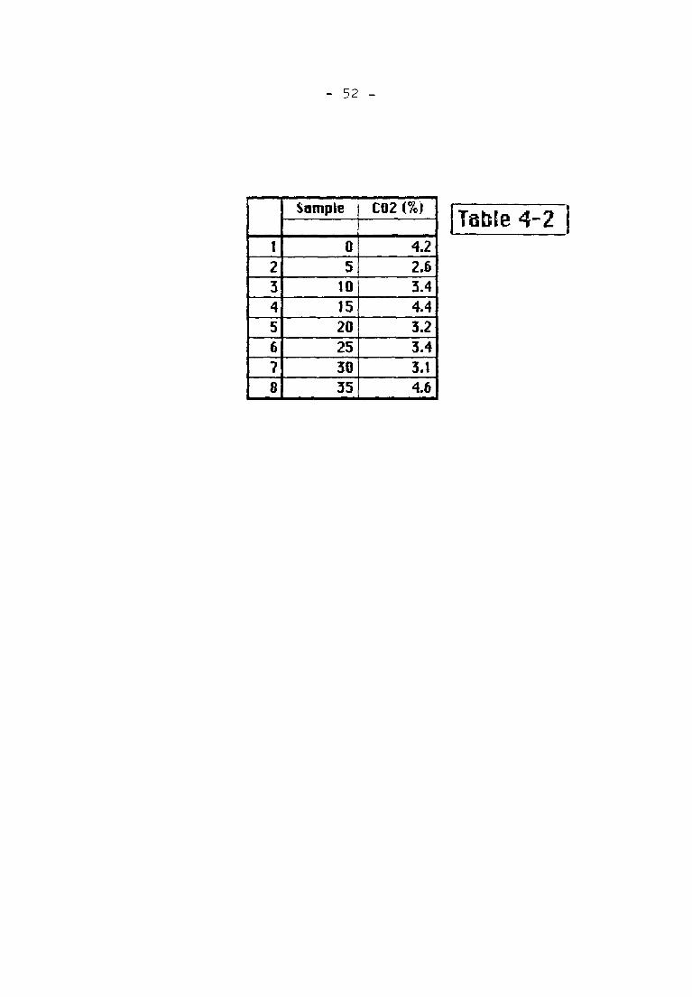
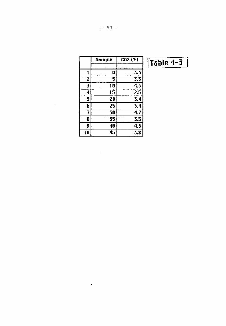
To verify this possibility, some CO2 mapping was done

along the perpendicular track which crosses the traverse

near the 90 site.

These measurements allow us to define some trends of

high and low CO2 levels, which are roughly N 80, i.e. the

direction identified on the ground where the fissures were

still evident (Tables 4-1, -2, -3) (Figure 34).

- 41 -

)

2

4

5

6

7

8

9

ta

tl

12

13

14

15

16

17

18

19

211

21

22

23

24

25

26

2?

2tt

29

30

31

32

33

34

35

36

3?

38

39

40

41

Al43

44

45

4A

47

48

49

Somplo

1 -14(1

-t30j

-120'

-lUI

-100

-90

-BD

-70

-60

-50

-40

-30

-20

-10

-fi

0

10

20

30

4tl

50

6R

70

BO

9U

lOQ

110

120

130

140

150

160

170

180

190

20U

210

220

230

240

250

260

270

280

290

300

310

32D

330

SP (mM>-Q8 1

3.8

5.6

1.5

1.0

-3.0E-1

-2.0E-1

-4.2

-2.1

8.0E-1

-6.9

-4.1

-3.6

-13.4

-6.1

-1Ü.2

-22.3

-15.5

-14.4

-13.4

-5.fi

-9.7

-8.5

-10.4

-9.3

-11.4

-n.6

-14.t

-17.4

-14.9

-12.4

-15.5

-14.3

-14.1

-14.2

-10.8

-7.4

-10.9

-8.2

^12.4

-14.4

-12.9

-9.5

-10.9

-14.0

-14.1

-20.8

C02 («.1-88-1

4.0

2.4

5.3

6.1

6.0

3.8

2.0

3.6

3.4

3.4

3.0

9.0E-1

3.5

4.9

3,5

5.7

3.3

2.7

3.6

4,0

4.0

3,2

3,4

3.3

3.7

3.4

4.6

3.2

4.0

3.4

2,9

3.6

5,2

3.5

4,7

4.t

3,2

4,7

5.4

5.1

9.3

4.9

3.5

3,3

3,9

2.B

3.8

2.1

3.5

Hn (pCi/M-B8-t

150

69

160

611

706

46t

235

152

267

209

287

61

221

34t

322

206

203

450

264

302

309

34!

365

299

306

206

380

507

376

409

232

365

365

170

215

380

396

245

412

229

256

J5a

150

304

227

176

253

144

412

cas i%) 9B-i

4.7

4.0

4.9~l

3.1

4.2

3,3

4.6

5.2

4.1

3.8

3.7

5.9

5.1

3,1

3.8

5.2

3.0

2.6

2.8

2,4

3,3

3.4

2,9

2,2

2,1

2,t

2.8

2.5

2.5

2.2

3.2

2.9

3.1

3,4

4.4

3.6

2.9

2.4

2.2

2.8

6.4

1.6

2.2

1.5

1.7

2.2

1.7

1,7

C03 (%) «9-3

5,2

5.7

4.4

5.0

6.1

3.0

5,0

6.3

4.9

4.3

3.6

6,5

5.0

2.2

3.7

4,8

3.9

2.6

2.8

2.8

4.0

2.1

2.4

3.3

3.0

2.5

2.8

2.9

3,7

2,5

3.5

2.7

4.0

3.0

3.7

3.5

3.0

3.2

1.9

4,0

7,2

3,1

4.1

3,8

3,2

2.1

4,1

S.D

4.1

Table 3

Rn (pti/O R6 ^

212

245

tl5

277

165

304

31B

217

117

383

65

274

136

145

305

253

306

278

223

236

296

770

206

236

60

1

2

55

90

220

185

269

211

232

302

273

103

76

137

102

60

210

32

76

40

133

74

35

42

15

124

He<ppm|60-2j

1

5.3

5.3

- 5.5

5.3

5,2

5.4

5.2

5,4

5.2

5.3

5.4

5.3

5.3

5.3

5,4

5.4

5.3

5.3

5.2

5.4

5.3

5.:<

5.4

5,3

5.3

_ 5.3

5.3

5,2

5,3

5,3

.

- k2

TJURAH BUNTU

C02

IOh

9

8

7.

6.

5.

4.

3.

2

1.

0.

\ Í

-150 -100

OC02 («)-88-1

1

\ 1 ^

0 î

!

-50 0 50 100

Sample

150

(95) 88-2

200 250 300 350

Feg,24

- A3 -

TJURAH BUNTU

(se) 88-2 DC02 (95) 88-3.

-111<- -I1 I1r -111 Ir-1

-150 -100 -50 0 50 1(K) 150 200 250 300 350

Sample

Fîg.25

A4 -

Tjuroh Buntu

Count

25-

20

15

10

5.

0. 1 J

0 1 :> 3 4 5 é

C02 (S?)-88-1

> 7 8

11

9

, 11 r

IC)

Pig.26

Count20 ' - .

18.

16

14.

12.

10

8

6-

4.

2

0

0 1 2 3 4 5

C02 m 88-2

7 8 9 10

Fig.27

-45 -

18t

16

14.

12

10.

2 8.

6.

4.

2.

0.

Tjuroh Buntu

01 23456789 IC

C02 (S5) 88-3

)

FÊg.28

- A6

TJURAH BUNTU

800 j

700.

600.

500.

Ç 400.

a.

2 300.

200.

100.

0.

-150

(pCi/1) 88-2

É

-100 -50 0

/^^

50 100

Sample

DRn (pCi/1)-88-l

^wu150 200 250

^

N300

f

350

Fig.29

A7 -

Tjurah Buntu

CM

00

00

CM

o

o

7

6.

5.

4.

3-

2.

1.

C

0

) 1

c9 0

0 0 °0 o

0

o 0

o ô 0

o^ô 0^ 00 0

*8 0 0° 0 9 0

0 0 0 ô 0 "

2 3-1567

C02 (%)-80-l

0

8 9 1 0

¡Flg.58

- 48 -

Tjurah Buntu

I

00

00

o

u

6.

,

0 o

%

0

0

^ 0

^°o

00/0

X

0

o

ô8^^0 0

Cto

0 _

0 0

11

0

o

1

0

0 y^

0 yy

0^°0

0

1 1 1

y".0

C02 (%) 80-2

ng.3t ]

- 49

Tjurah Buntu

800

700

600J

1

88-Ô

&

500

400

300

200

100

0

- o

-11r- -11r

4 5 6

C02 (?.)-08-1

I

9 10

FiS-32

- 50 -

Tjurah Buntu

CM1

00

00

ôu.N^

c

ct

400

350.

300.

250.

200.

150-

100.

50-

0

1

o

cP

Oo

0

0 0

0 0

0

0

0

0

0 y

00

0

2

0 /

o/ooog 0 y

0 © // o c.

0 /

^ 0 / 0 0

y^ 0

X ° 0 °o_o

1 1 1 1 1

3 4 5

C02 (%) 08-2

0

0

1 '

6 7

[Fig.35

- 51 -

1

2

3

4

5

6

7

8

9

10

It

12

13

14

15

16

17

18

19

20

21

22

23

24

Sample

0

10

15

20

25

30

35

40

45

50

55

60

65

70

75

80

85

90

95

100

105

110

115

120

C02 (%)

2.9

2.5

2.3

2.7

2.5

2.9

2.5

1.5

3.7

2.9

3.6

4.3

3.2

3.4

5.5

3.2

3.1

4.2

2.2

2.7

3.2

3.7

3.5

. 3.3

Table 4-1

52 -

1

2

3

4

5

6

7

8

Sample

0

5

10

15

20

25

30

35

COZ (%)

4.2

2.6

3.4

4.4

3.2

3.4

3.1

4.6

Teble 4-2

- 53 -

1

2

3

4

5

6

7

8

9

10

Sample

0

5

10

15

20

25

30

35

40

45

COZ (%)

3.3

3.3

4.3

2.5

3.4

3.4

4.7

3.5

4.3

3.8

Tsble 4-5 1

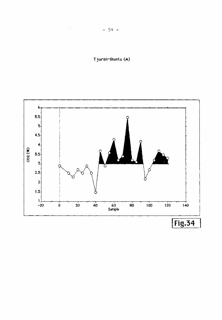
- 54

Tjurah-Buntu (A)

6

5.5

5

4.5

4

\^

CM ^-^

2.5

2.

1.5.

1 I1 11111 I1111111

-20 0 20 40 60 80 100 120 140

Sample

Fig.34

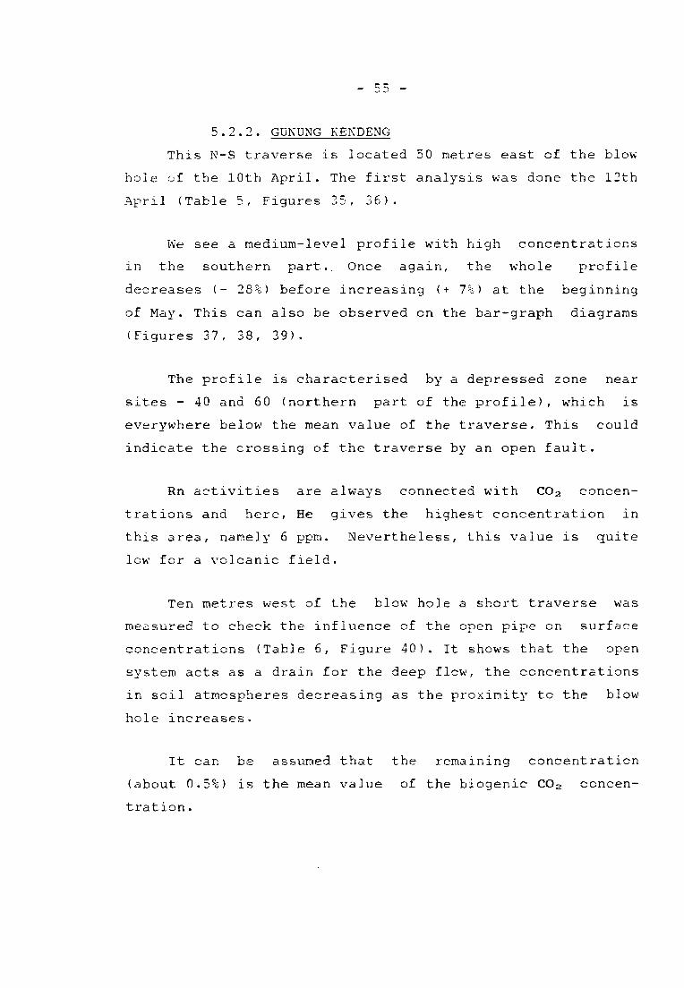
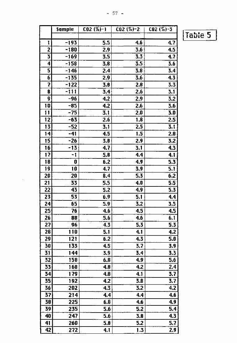
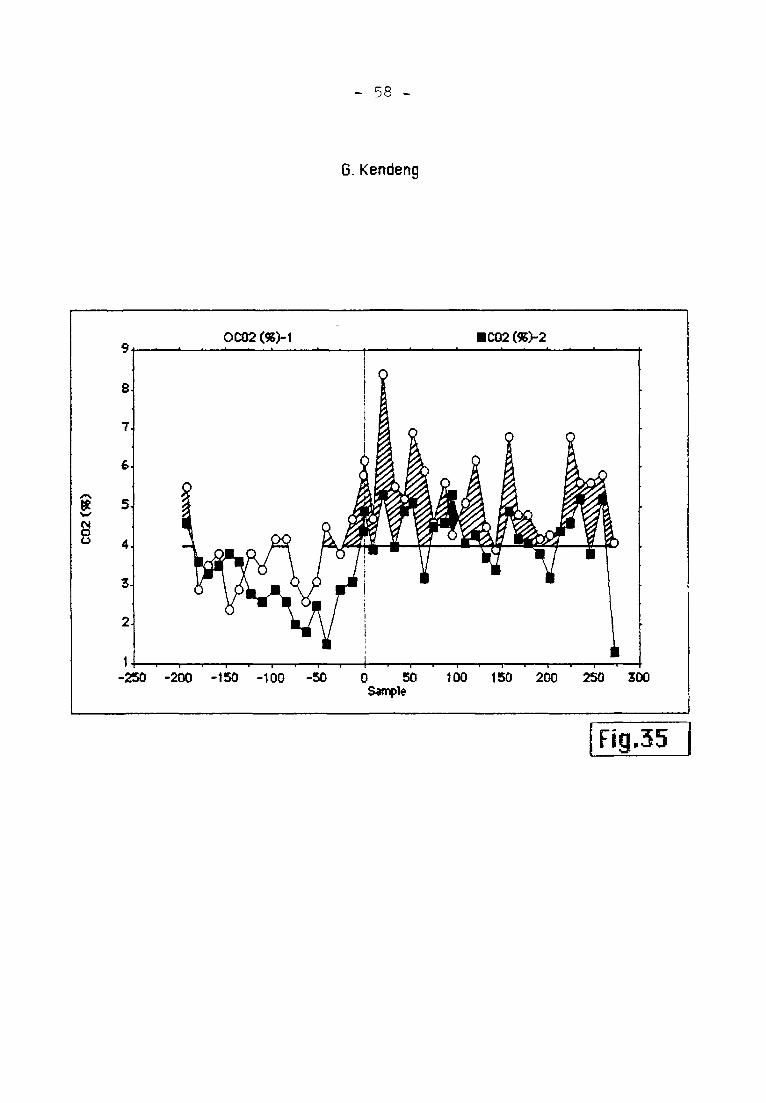
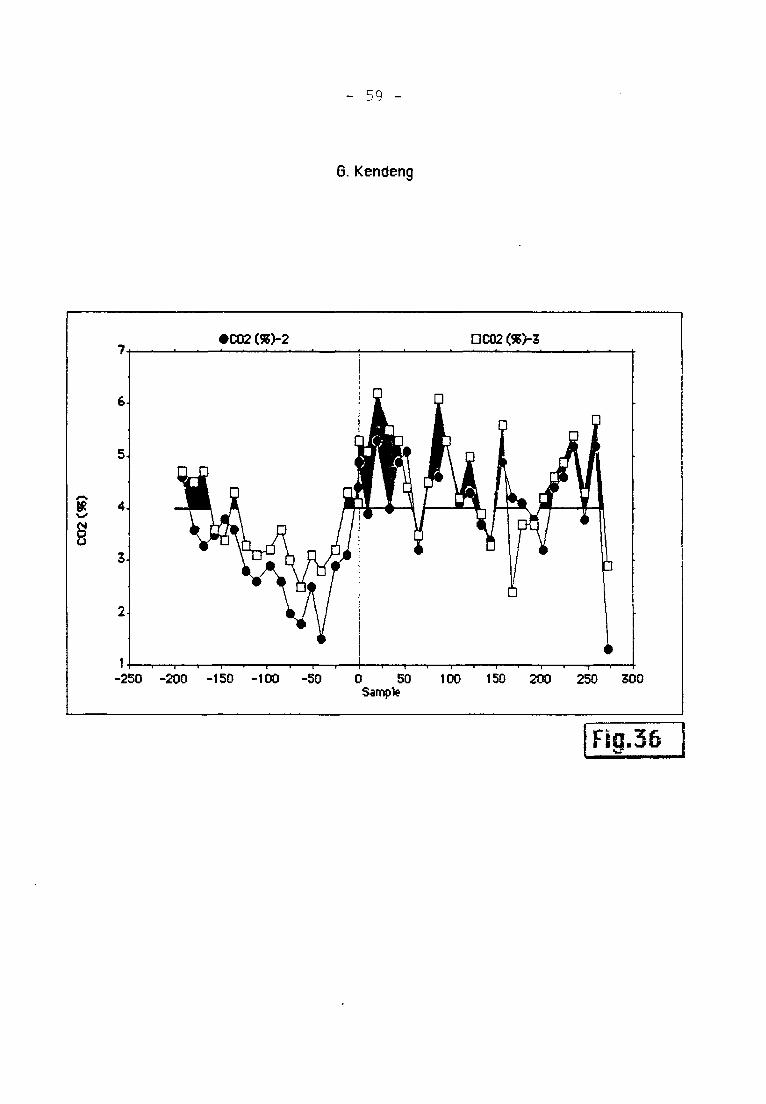
5.2.2. GUNUNG KENDENG

This N-S traverse is located 50 metres east cf the blow

hole of the 10th April . The first analysis was done the 12th

April (Table 5, Figures 35, 36).

We see a medium-level profile with high concentrations

in the southern part.. Once again, the whole profile

decreases (- 28%) before increasing (+ 7%) at the beginning

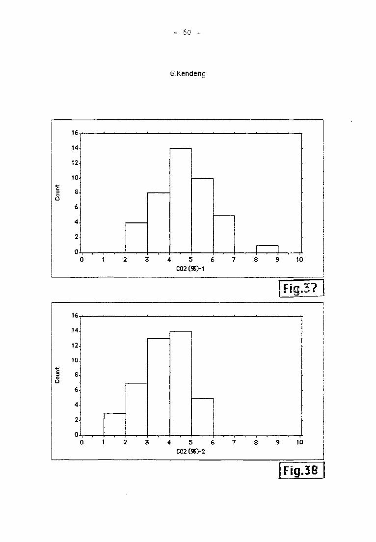
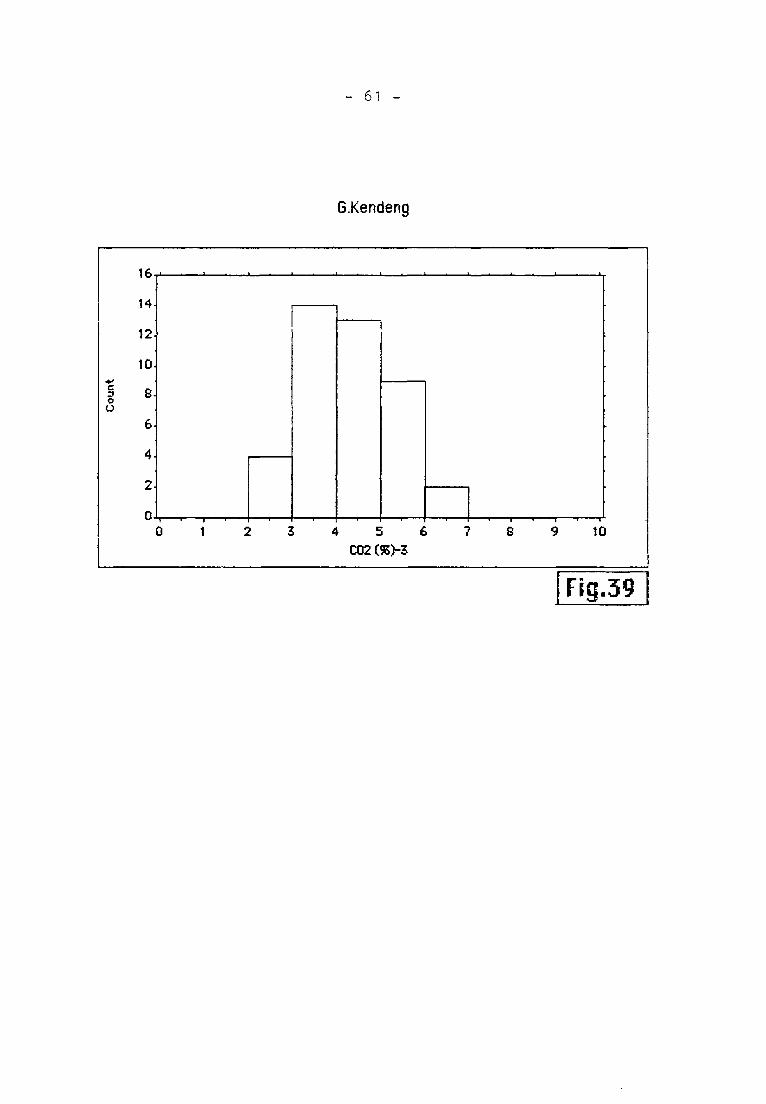
of May. This can also be observed on the bar-graph diagrams

(Figures 37, 38, 39).

The profile is characterised by a depressed zone near

sites - 40 and 50 (northern part of the profile), which is

everywhere below the mean value of the traverse. This could

indicate the crossing of the traverse by an open fault.

Rn activities are always connected with COa concen¬

trations and here. He gives the highest ccncentration in

this area, namely 6 ppm. Nevertheless, this value is quite

lew for a volcanic field.

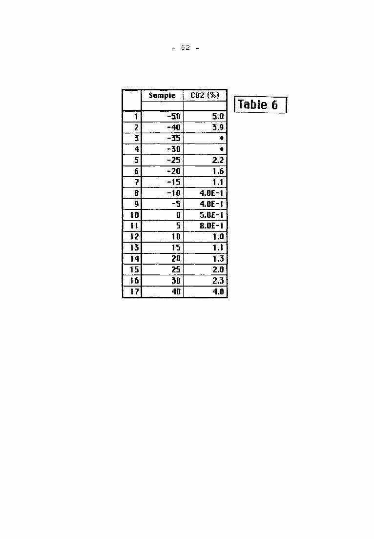
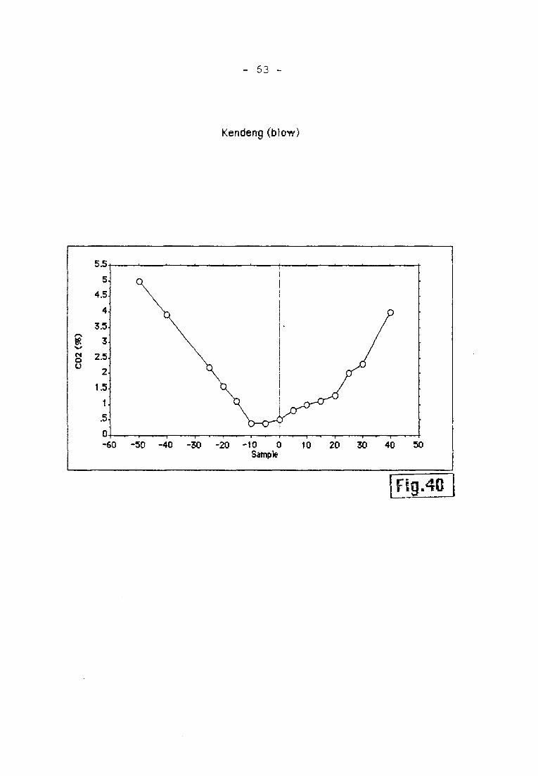
Ten metres west of the blow hole a short traverse was

measured to check the influence of the open pipe on surface

concentrations (Table 6, Figure 40). It shows that the open

system acts as a drain for the deep flow, the concentrations

in soil atmospheres decreasing as the proximity to the blow¬

hole increases.

It can be assumed that the remaining concentration

(about 0.5%) is the mean value of the biogenic CO2 concen¬

tration .

= 6 -

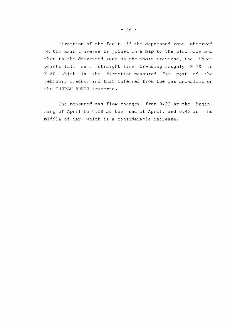
Direction of the fault. If the depressed zone observed

on the main traverse is joined on a map to the blow hole and

then to the depressed zone on the short traverse, the three

points fall on a straight line trending roughly N 70 to

N 80, which is the direction measured for most of the

February cracks, and that inferred from the gas anomalies on

the TJURAH BUNTU traverse.

The measured gas flow changes from 0.22 at the begin¬

ning cf April tc 0.18 at the end of April, and 0.45 in the

middle of May, which is a considerable increase.

- 57 -

1

2

3

4

5

6

7

8

9

10

11

12

13

14

15

16

17

18

19

20

21

22

23

24

25

26

27

28

29

30

31

32

33

34

35

36

37

38

39

40

41

42

Sample

-193

-180

-169

-158

-146

-135

-122

-111

-96

-85

-75

-63

-52

-41

-26

-13

-1

0

10

20

33

43

53

65

76

88

96

110

121

133

144

158

168

179

192

202

214

225

235

247

260

272

COZ(%)-í

5.5

2.9

3.5

3.8

2.4

2.9

3.8

3.4

4.2

4.2

3.1

2.6

3.1

4.5

3.8

4.7

5.8

6.2

4.7

8.4

5.5

5.2

6.9

5.9

4.6

5.6

4.3

5.1

6.2

4.5

3.9

6.8

4.8

4.8

4.2

4.3

4.4

6.8

5.6

5.6

5.8

4.1

COZ (%)-2

4.6

3.6

3.3

3.5

3.8

3.6

2.8

2.6

2.9

2.6

2.0

1.8

2.5

1.5

2.9

3.1

4.4

4.9

3.9

5.3

4.0

4.9

5.1

3.2

4.5

4.6

5.3

4.1

4.3

3.7

3.4

4.9

4.2

4.1

3.8

3.2

4.4

4.6

5.2

3.8

5.2

1.3

COZ (%)-3

4.7

4.5

4.7

3.6

3.4

4.3

3.3

3.1

3.2

3.6

3.0

2.5

3.1

2.8

3.2

4.3

4.1

5.3

5.1

6.2

5.5

5.3

4.4

3.5

4.5

6.1

5.3

4.2

5.0

3.9

3.3

5.6

2.4

3.7

3.7

4.2

4.6

4.9

5.4

4.3

5.7

2.9

^ Table 5

- 58 -

G. Kendeng

C02

Qj

8

7.

6

5.

4

3.

2-

1-

-250 -200

OC02 («)-1

-150 -100

loif j

-50 (

m \ /V /

) 50

Sample

(95)-2

100 150 200 250 300

Fig.35

- 59 -

G. Kendeng

o

(SS)-2 DC02 (SB)-3

Fig,56

- 60 -

G.Kendeng

Count

16,

14-

12

10

8

6.

4.

2

0.Ill'

0 1 2ï 3 4 5 6 7

C02 (S5)-1

8 9 IC

iFrg

)

,3?

Count](^ .......... .

14

12

10

8.

6.

4.

2

0.

0 1 2 3 4 5 é

C02 (95)-2

7

I

8

;

1

!

1 . 1

9 10

-

Fig,38

61 -

G.Kendeng

Couni

]Ç^ ............ .

14.

12.

10

8.

6.

4.

2.

0.(J."! 1 1 1 1 1 1 I 1

0 1 2 3 4 5 6 "3

C02(«)-3

00-1 'T'1

9 10

.

Fig.39

- 62

1

2

3

4

5

6

7

8

9

10

11

12

13

14

15

16

17

Sample

-50

-40

-35

-30

-25

-20

-15

-10

-5

0

5

10

15

20

25

30

40

COZ (%)

5.0

3.9

2.2

1.6

1.1

4.0E-1

4.0E-1

5.0E-1

8.QE-1

1.0

1.1

1.3

2.0

2.3

4.0

Table 6

- 63

Kendeng (blow)

C02

55

5.

4.5.

4.

3.5.

3.

2.5.

2

1.5.

1.

.5.

0.

-60 -50 -40 -30 -20 -10 c

Sample

) 10 20 30 40 50

Fig.40

- 64 -

6. GENERAL INTERPRETATION

6.1. Flows of gas

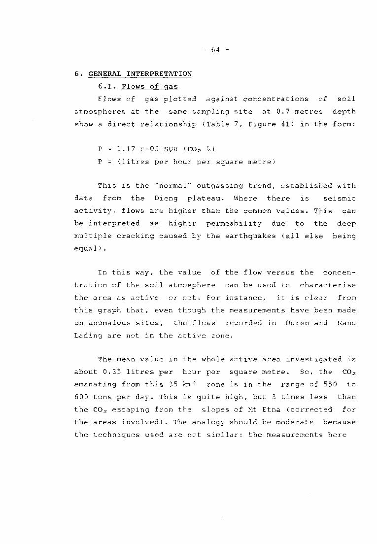
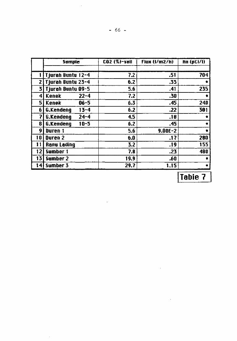
Flows of gas plotted against concentrations of soil

atmospheres at the same sampling site at 0.7 metres depth

show a direct relationship (Table 7, Figure 41) in the form:

P = 1.17 E-03 SQR (COz %. )

P = (litres per hour per square metre)

This is the "normal" outgassing trend, established with

data from the Dieng plateau. Where there is seismic

activity, flows are higher than the common vâlues. This can

be interpreted as higher permeability due to the deep

multiple cracking caused by the earthquakes (all else being

equal ) .

In this way, the value of the flow versus the concen¬

tration cf the soil atmosphere can be used tc characterise

the area as active or not. For instance, it is clear from

this graph that, even though the measurements have been made

on anomalous sites, the flows recorded in Duren and Ranu

Lading are not in the active zone.

The mean value in the whole active area investigated is

about 0.35 litres per hour per square metre. So, the CO2

emanating from this 35 km- zone is in the range cf 550 to

600 tons per day. This is quite high, but 3 times less than

the CO2 escaping from the slopes cf Mt Etna (corrected for

the areas involved). The analogy should be moderate because

the techniques used are not similar: the measurements here

- 6;

are made in a static mode, whereas on Etna it was made in a

dynamic mode. The latter should give higher values. For

comparison, the mean value calculated here is half that of

the escape from the cold area into the active crater of La

Sulfatara (Flegrean fields - Italy). Measurements made in

the same way give flows of about 0.03 1 m~^.h~^ to 0.06 1

m~^.h~^ for the biogenic activity in a forest located on

volcanic soil (Vesuvius volcano, Italy).

- 66 -

1

2

3

4

5

6

7

8

9

10

11

12

13

14

Sample

Tjurah Buntu 12-4

Tjurah Buntu 23-4

Tjurah Buntu 09-5

Kenek 22-4

Kenek 06-5

G.Kendeng 13-4

B.Kendeng 24-4

G.Kendeng 10-5

Duren 1

Duren 2

Ranu Lading

Sumber 1

Sumber 2

Sumber 3

COZ (%)-soil

7.2

6.2

5.6

7.2

6.3

6.2

4.5

6.2

5.6

6.0

3.2

7.8

19.9

29.7

FluK O/mZ/'h)

.51

.33

.41

.30

.45

.22

.18

.45

9.00E-2

.17

.19

.23

.60

1.15

Rn (pCi/0

704

235

t

240

301

280

155

480

Table ?

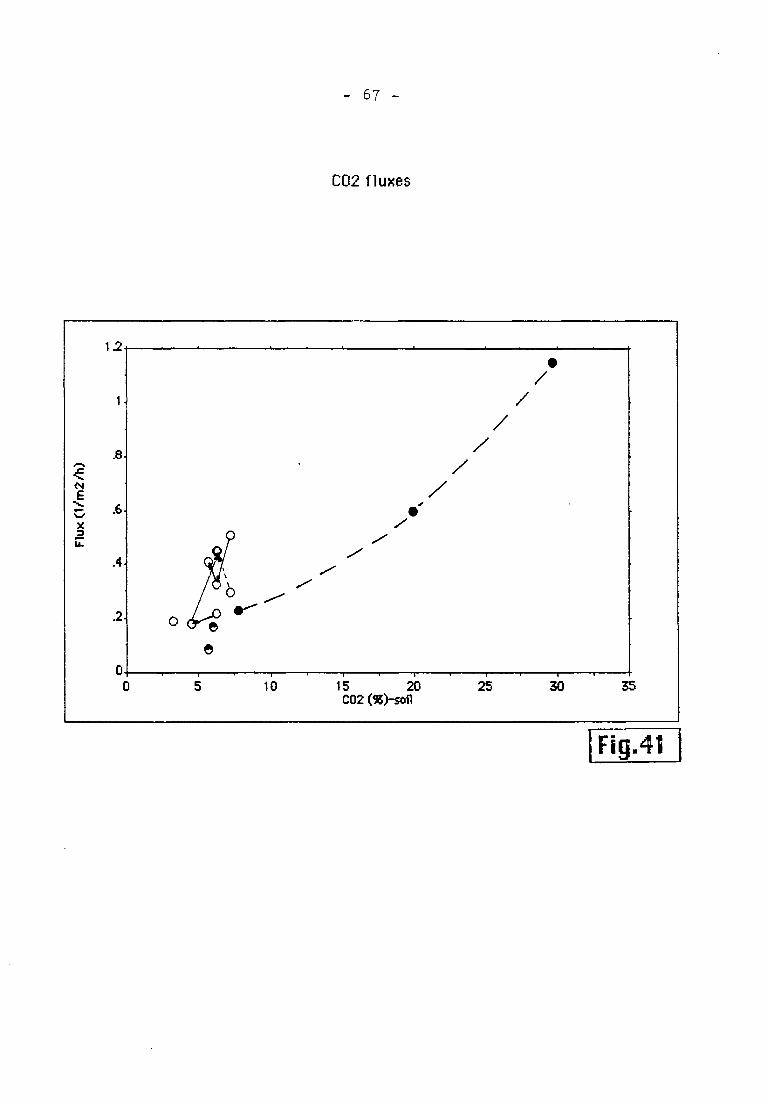
- 67

C02 fluxes

- 68 -

6.2. Profiles

- Traverses give the places where flow measurements

should be done (on anomalies).

- Traverses give the locations of faults (fractures areas

with high permeabilities).

- Traverses give the places where the cracks are located,

even if they vanish due to the heavy rain showers.

- Traverses give a quick appreciation of the deep gas

flow variation within time, because concentrations and

flows are closely linked for a particular site. A 1500

to 2000 m traverse can easily be done in a day whereas

a single flux measurement needs 6 hours or more at the

same place.

6.3. Concentrations

CO2 : in this area there has been a large increase of

deep gas exhaust since last year. This could be connected

with the February crisis.

CO2 concentrations reach the limits of dangerous levels

according tc the data obtained on Dieng plateau. 9% CO2 in

soil atmospheres means that high concentrations exist

withing a few hundred metres of the surface. These large

volumes of CO2 could be rapidly released during a seismic

crisis with the related risks: small to large blows with

mechanical effects, toxicity of CO^ , etc.

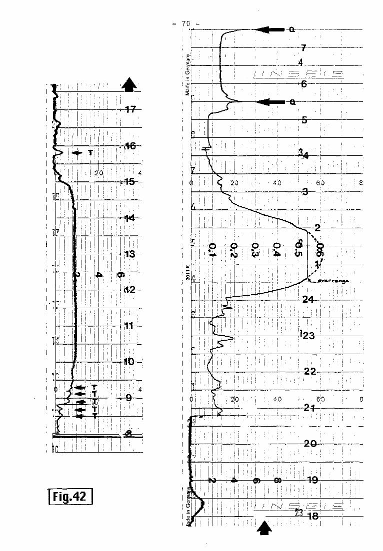
CO2 concentrations (and flows) are linked with seismic

activity: the minor crisis observed at the beginning cf May

corresponds with an increase in gas. Moreover, a short

period of monitoring of CO2 in the blow hole has shown that

variations in CO2 were linked with seismic noises (or

tremors): see figure 42 with explanations.

Ranu Pakis is a maar lake located on the very active

KENEK-1 fault system. As it is about 150 metres deep and the

fault system delivers large quantities of gas, this lake

could soon be very dangerous, acting as an enormous CO2

reservoir .

Rn: Rn is associated with CO2 , therefore the process

involved here is a hot water system.

He: there are no high concentrations of He (about

10 ppm or more) in the areas investigated. We can

therefore infer that at the localities where the

analyses were run there is no evidence of an underlying

magmatic intrusion.

But, it should be remembered that whereas CO2 and Rn

give large or very large haloes. He will give only a narrow

anomaly if the source is a dyke. In such a case, a traverse

must be made across the system.

- 70 -

! ' I

i i2o; ¡

i

^46^

4S^

-^

^

io>

-*^

^

^

I 1 1

Fig,42

tu

1

; ' ;-i .': : i

; ' 1 ' 1

[ ' ' ' ,

1 '

!' : : 4

'\' '.il i<-J ^_. L

. c

¡

- 71 -

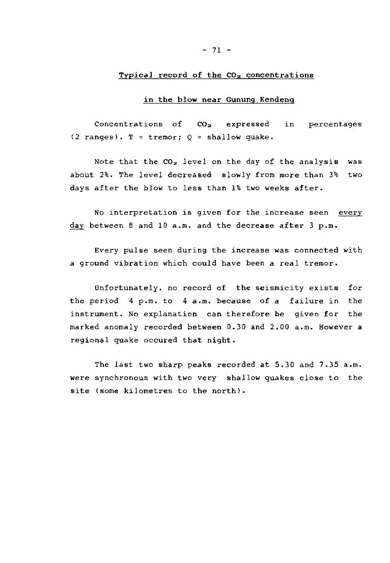
Typical recorci of the CO2 concentrations

in the blow near Gunung Kendeng

Concentrations of CO2 expressed in percentages

(2 ranges). T = tremor; Q = shallow quake.

Note that the CO2 level on the day of the analysis was

about 2%. The level decreased slowly from more than 3% two

days after the blow to less than 1% two weeks after.

No interpretation is given for the increase seen every

day between 8 and 10 a.m. and the decrease after 3 p.m.

Every pulse seen during the increase was connected with

a ground vibration which could have been a real tremor.

Unfortunately, no record of the seismicity exists for

the period 4 p.m. to 4 a.m. because of a failure in the

instrument. No explanation can therefore be given for the

marked anomaly recorded between 0.30 and 2.00 a.m. However a

regional quake occured that night.

The last two sharp peaks recorded at 5.30 and 7.35 a.m.

were synchronous with two very shallow quakes close to the

site (some kilometres to the north).

- 72 -

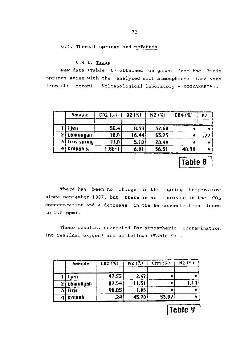
6.4. Thermal springs and mofettes

6.4.1. Tiris

New data (Table 8) obtained on gases from the Tiris

springs agree with the analysed soil atmospheres (analyses

from the Merapi - Volcanological laboratory - YOGYAKARTA) .

1!

2

3

4

Sample

ijen

Lamongan

Tiris spring

Kolbah s.

C02 (%)

58.4

16.8

77.8

1.8E-1

02 (%)

8.38

16.44

5.tÜ

6.01

N2 (%}

32.60

65.25

2Ü.4y

56.51

CH4 (%)

*

40.30

K2

.22

¡Tables

There has been no change in the spring temperature

since September 1987, but there is an increase in the CO2

concentration and a decrease in the He concentration (down

to 2.5 ppm ) .

These results, corrected for atmospheric contamination

(no residual oxygen) are as follows (Table 9) .

1

2

3

4

SdmpEb

Ijen

Lamongan

Tiris

Kolbah

coz (%)

97.53

87.54

98.05

.24

N2 (%)

2.47

11.31

1.95

45.70

CH4 í%)

53.97

HZ {%)

1

1.14

Table 9

- 73 -

1

2

3

4

5

6

7

8

9

10

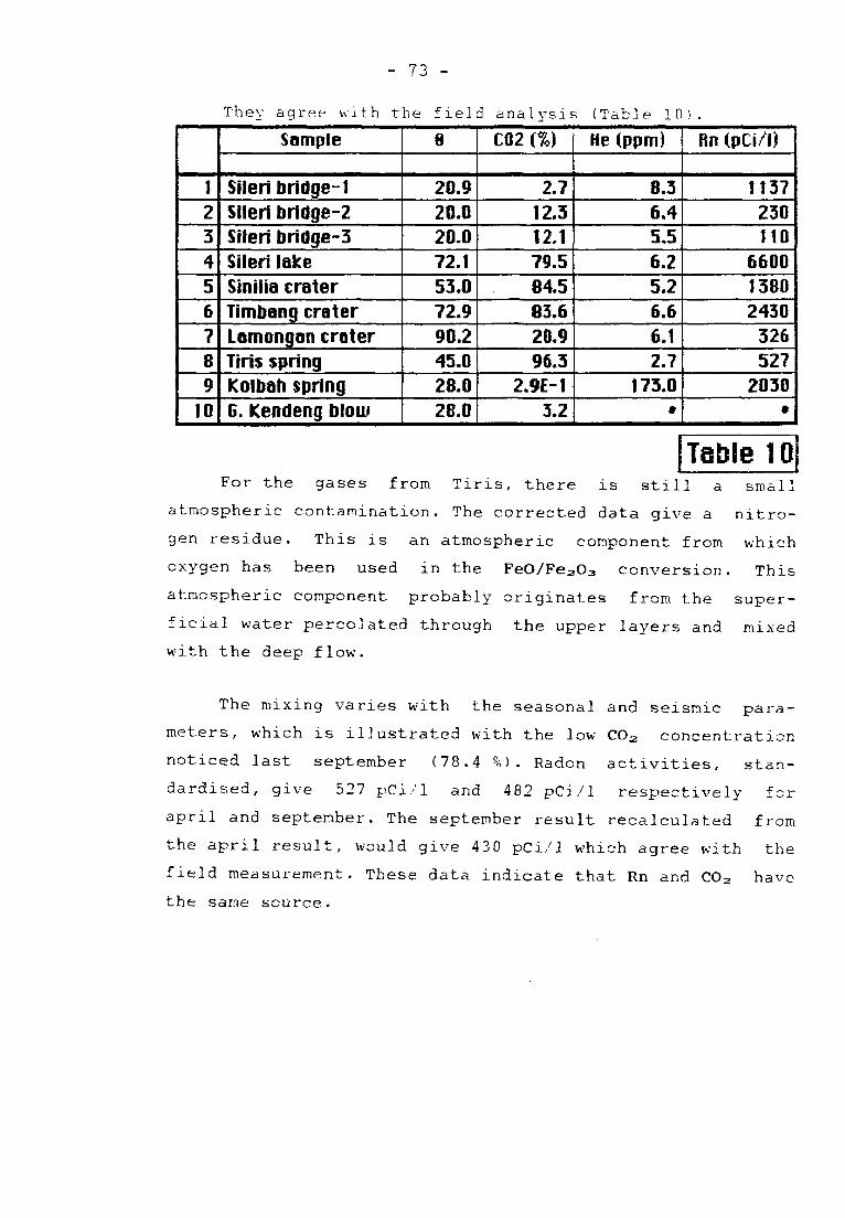
They agree with the field analysis

Sample

Sileri bridge- 1

Sileri brldge-2

Sileri bridge-3

Sileri lake

Sinilia crater

Timbang crater

Lamongan crater

Tiris spring

Kolbah spring

G. Kendeng blow

6

20.9

20.0

20.0

72.1

53.0

72.9

90.2

45.0

28.0

28.0

C02 (%)

2.7

12.3

12.1

79.5

84.5

83.6

20.9

96.3

2.9E-1

3.2

3 (Table 10) .

He (ppm)

8.3

6.4

5.5

6.2

5.2

6.6

6.1

2.7

173.0

Rn (pCi/l)

1137

230

110

6600

1380

2430

326

527

2030

Table 10

For the gases from Tiris, there is still a small

atmospheric contamination. The corrected data give a nitro¬

gen residue. This is an atmospheric component from which

oxygen has been used in the FeO/FezOa conversion. This

atmospheric component probably originates from the super¬

ficial water percolated through the upper layers and mixed

with the deep flow.

The mixing varies with the seasonal and seismic para¬

meters, which is illustrated with the low CO2 concentration

noticed last September (78.4 %). Radon activities, stan¬

dardised, give 527 pCi/1 and 482 pCi/1 respectively for

april and September. The September result recalculated from

the april result, would give 430 pCi/1 which agree with the

field measurement. These data indicate that Rn and CO2 have

the same source .

- 74 -

This can be explained by an input of shallow CO2 into

the area where the water table is heated. Either the new

input of energy is of shallow origin, or the thermal water

has a lateral source, possibly a connection with the active

area. On the latter hypothesis. He will not be carried along

with water.

6.4.2. Kolbah

The Kolbah spring, located ESE of the volcano (Tanggul

sheet, half way between Kaliboto 3 and Kotokan 1) rises at a

normal temperature in a small pool without any ferrous oxide

deposit .

The gas analysis, recalculated, gives a very surprising

result: the gas is half N2 and half CH* with a high He

concentration (173 ppm). CO2 is a minor constituent: only

0.29%. The theoretical composition of the gas (0.24% CO2 )

agrees with the field CO2 measurement. Such a mixture of

gases has sometimes been found on faults that are probably

very deep, which could be the case here.

6.4.3. Lamongan

Fumaroles from the Lamongan summit will contain only

10 ppm of He in the dry gas (87.5% of CO2 ) . This value is

very common in a quiescent volcanic period. It is the only

sample analysed which contains hydrogen. The 6^^C%o gives an

intermediate value: -2.4 and -2.9 ± 0.1. This can be

explained by a mixture between deep carbon and carbon from

carbonates of the crust. Values in the same range have been

found before by P. ALLARD (1986) in gases of Ijen, Merapi

and Central American Volcanoes.

- 75 -

7. CONCLUSION

The area investigated as a monitoring example shows

a large input of heat, carried up by water. There is no

magmatic evidence for the system in this particular area.

However, the four traverses where the analyses have

been conducted do not allow a general verdict for the whole

area. Ivestigations should be made soon on traverses close

to the seismic epicentres to confirm this conclusion.

8. RECOMMENDATIONS

- Measurements should be repeated every two months to

understand clearly the phenomena.

- A geochemical map should be drawn to avoid working on

irrelevant areas. A 20 to 25 m interval is suggested.

- Frequent He measurements should be made to check the

magmatic input, which can change very quickly: He will

change with magma ascent, but CO2 and Rn will probably

change more slowly because they are connected with

water. This needs modern instruments to obtain accurate

data .

- Permanent monitoring over medium to long periods should

be done for Rn and CO2. If H2 can be linked with He

escape, it will be a good tracer.

- As an important input of heat exists somewhere,

attested by gas escape, shallow waters must.be heated

(in the range of some tens of degrees); Since the area

is confined, this cannot be done without an uplift. The

three lakes (Ranu Pakis, Lamongan and Bedali) should be

used as large integrating tiltmeters. Light automatic

equipment is commercially available for this purpose

(3 sensors per lake).

- 76 -

The depth of Ranu Pakis should be checked and the

gas/water ratio measured in the deepest water layers.

A general survey of the depths of all the lakes should

be made to obtain a general idea of the risk of

outgassing of water.

methodology for the geochemical monitoring of an active ...

Documents