Meta-analysis in Stata: history, progress and prospects · 2005-07-19 · Meta-analysis in Stata: history, progress and prospects Jonathan Sterne Department of Social Medicine University

Meta-analysis in Stata:history, progress and prospects

Jonathan SterneDepartment of Social Medicine

University of Bristol, UK

Outline

• Systematic reviews and meta-analysis• Meta-analysis in Stata• Bias in meta-analysis• Stata commands to investigate bias• Present situation• The Future……

Systematic reviews• Systematic approach to minimize biases and random

errors• Always includes materials and methods section• May include meta-analysis

Chalmers and Altman 1994

Meta-analysis• A statistical analysis which combines the results of

several independent studies considered by the analyst to be ‘combinable’

Huque 1988

Streptokinase (thrombolytic therapy)• Simple idea if we can dissolve the blood clot causing

acute myocardial infarction then we can save lives• However – possible serious side effects• First trial - 1959

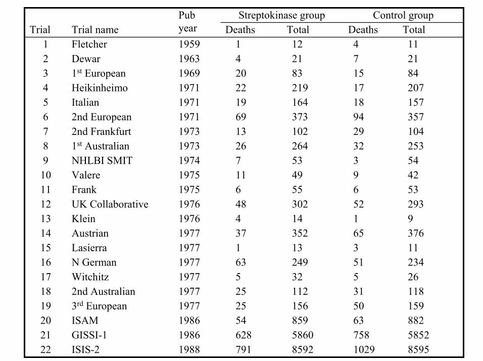
102975863503155136515269332299418171574

DeathsControl group

85925860859156112322491335214302554953264102373164219832112

Total

85957911988ISIS-22258526281986GISSI-121882541986ISAM201592519773rd European191182519772nd Australian182651977Witchitz17234631977N German161111977Lasierra15376371977Austrian14941976Klein13293481976UK Collaborative125361975Frank1142111975Valere105471974NHLBI SMIT92532619731st Australian81041319732nd Frankfurt73576919712nd European6157191971Italian5207221971Heikinheimo4842019691st European32141963Dewar21111959Fletcher1

TotalDeathsPub yearTrial nameTrial

Streptokinase group

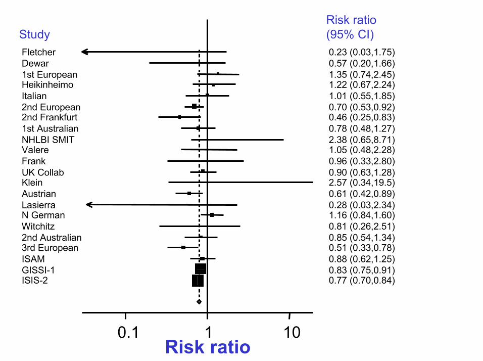
StudyRisk ratio (95% CI)0.23 (0.03,1.75)Fletcher0.57 (0.20,1.66)Dewar1.35 (0.74,2.45)1st European1.22 (0.67,2.24)Heikinheimo1.01 (0.55,1.85)Italian0.70 (0.53,0.92)2nd European0.46 (0.25,0.83)2nd Frankfurt0.78 (0.48,1.27)1st Australian2.38 (0.65,8.71)NHLBI SMIT1.05 (0.48,2.28)Valere0.96 (0.33,2.80)Frank0.90 (0.63,1.28)UK Collab2.57 (0.34,19.5)Klein0.61 (0.42,0.89)Austrian0.28 (0.03,2.34)Lasierra1.16 (0.84,1.60)N German0.81 (0.26,2.51)Witchitz0.85 (0.54,1.34)2nd Australian0.51 (0.33,0.78)3rd European0.88 (0.62,1.25)ISAM0.83 (0.75,0.91)GISSI-10.77 (0.70,0.84)ISIS-2

Risk ratio0.1 1 10

Archie Cochrane (1979)

“ It is surely a great criticism of our profession that we have not organized a critical summary, by specialty or subspecialty, adapted

periodically, of all relevant randomized controlled trials ”

The Cochrane Collaboration• “An international organization that aims to help people make well

informed decisions about health care by preparing, maintaining and ensuring the accessibility of systematic reviews of the effects of health care interventions”– Ten principles: collaboration, building on the enthusiasm of individuals,

avoiding duplication, minimizing bias, keeping up to date, striving for relevance, promoting access, ensuringquality, continuity, enabling wide participation

• To date, more than 3000 reviews or protocolsfor reviews have been published, and a database of more than 375,000 trials has been accumulated

• See www.cochrane.org

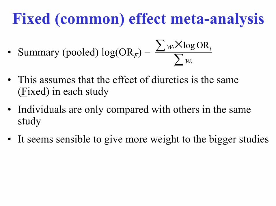
Fixed (common) effect meta-analysis

• Summary (pooled) log(ORF) =∑

∑ ×w

wi

ii OR log

• This assumes that the effect of diuretics is the same (Fixed) in each study

• Individuals are only compared with others in the same study

• It seems sensible to give more weight to the bigger studies

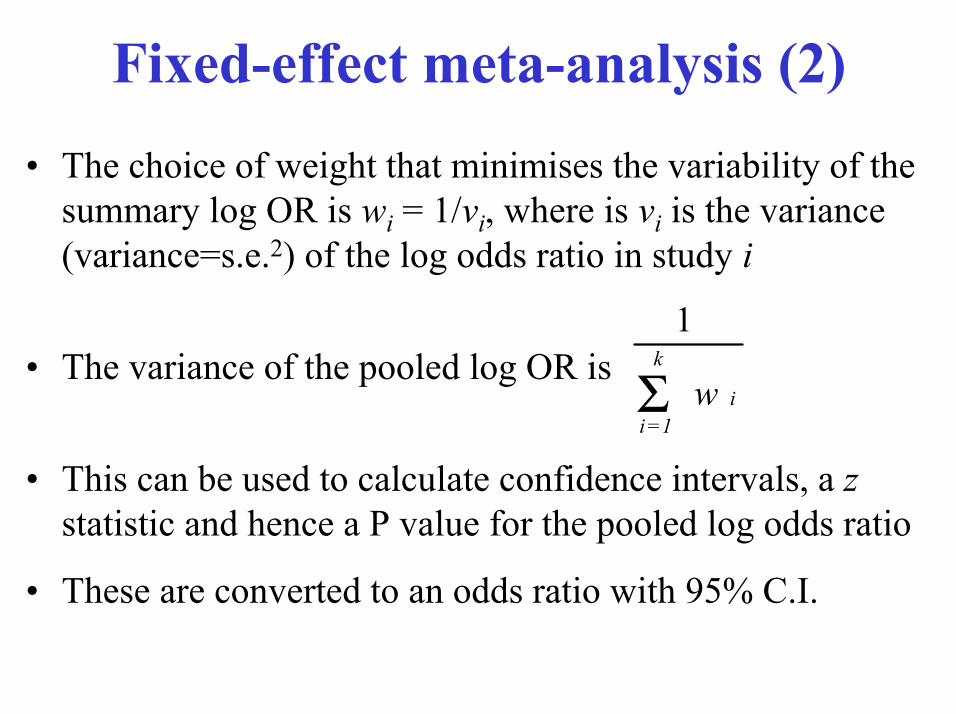
• The choice of weight that minimises the variability of the summary log OR is wi = 1/vi, where is vi is the variance (variance=s.e.2) of the log odds ratio in study i

• The variance of the pooled log OR is

• This can be used to calculate confidence intervals, a zstatistic and hence a P value for the pooled log odds ratio

• These are converted to an odds ratio with 95% C.I.

Fixed-effect meta-analysis (2)

w i

k

=1iΣ

1

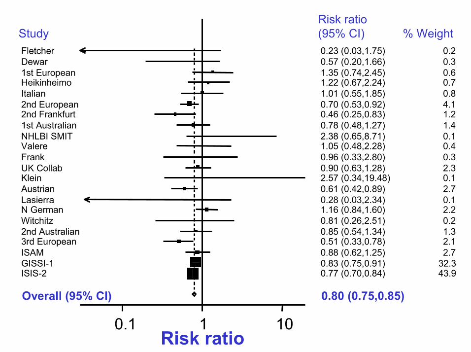
StudyRisk ratio (95% CI)0.23 (0.03,1.75)Fletcher0.57 (0.20,1.66)Dewar1.35 (0.74,2.45)1st European1.22 (0.67,2.24)Heikinheimo1.01 (0.55,1.85)Italian0.70 (0.53,0.92)2nd European0.46 (0.25,0.83)2nd Frankfurt0.78 (0.48,1.27)1st Australian2.38 (0.65,8.71)NHLBI SMIT1.05 (0.48,2.28)Valere0.96 (0.33,2.80)Frank0.90 (0.63,1.28)UK Collab2.57 (0.34,19.48)Klein0.61 (0.42,0.89)Austrian0.28 (0.03,2.34)Lasierra1.16 (0.84,1.60)N German0.81 (0.26,2.51)Witchitz0.85 (0.54,1.34)2nd Australian0.51 (0.33,0.78)3rd European0.88 (0.62,1.25)ISAM0.83 (0.75,0.91)GISSI-10.77 (0.70,0.84)ISIS-2

% Weight0.20.30.60.70.84.11.21.40.10.40.32.30.12.70.12.20.21.32.12.7

32.343.9

0.80 (0.75,0.85)Overall (95% CI)

Risk ratio0.1 1 10

Forest plots• Boxes draw attention to the studies with the greatest

weight

• Box area is proportional to the weight for the individual study

• The diamond (and broken vertical line) represents the overall summary estimate, with confidence interval given by its width

• Unbroken vertical line is at the null value (1)

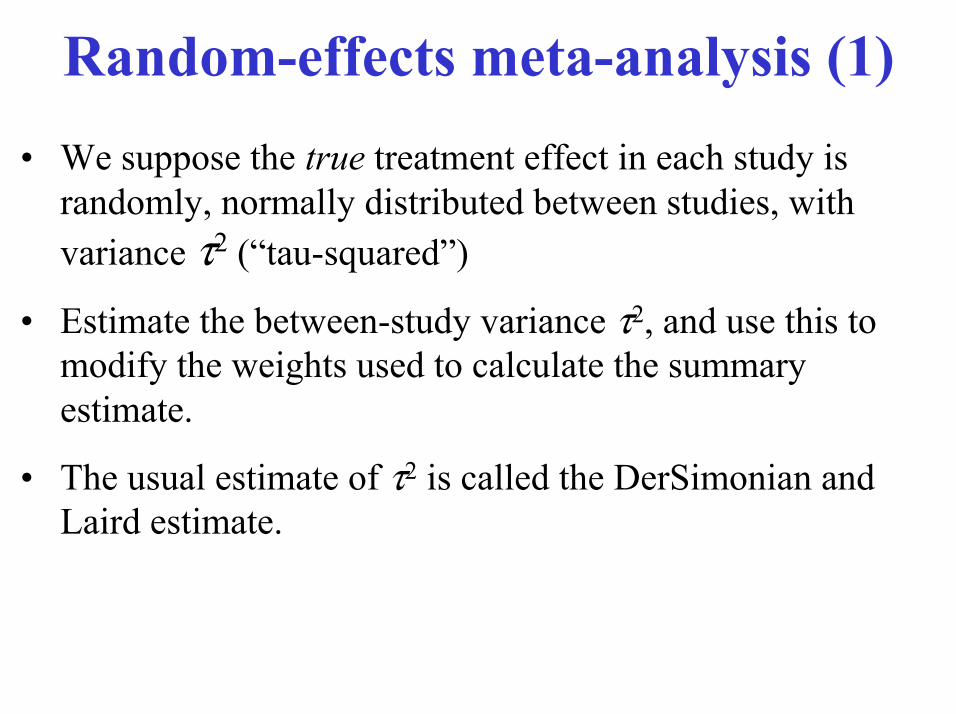
Random-effects meta-analysis (1)• We suppose the true treatment effect in each study is

randomly, normally distributed between studies, with variance τ2 (“tau-squared”)

• Estimate the between-study variance τ2, and use this to modify the weights used to calculate the summary estimate.

• The usual estimate of τ2 is called the DerSimonian and Laird estimate.

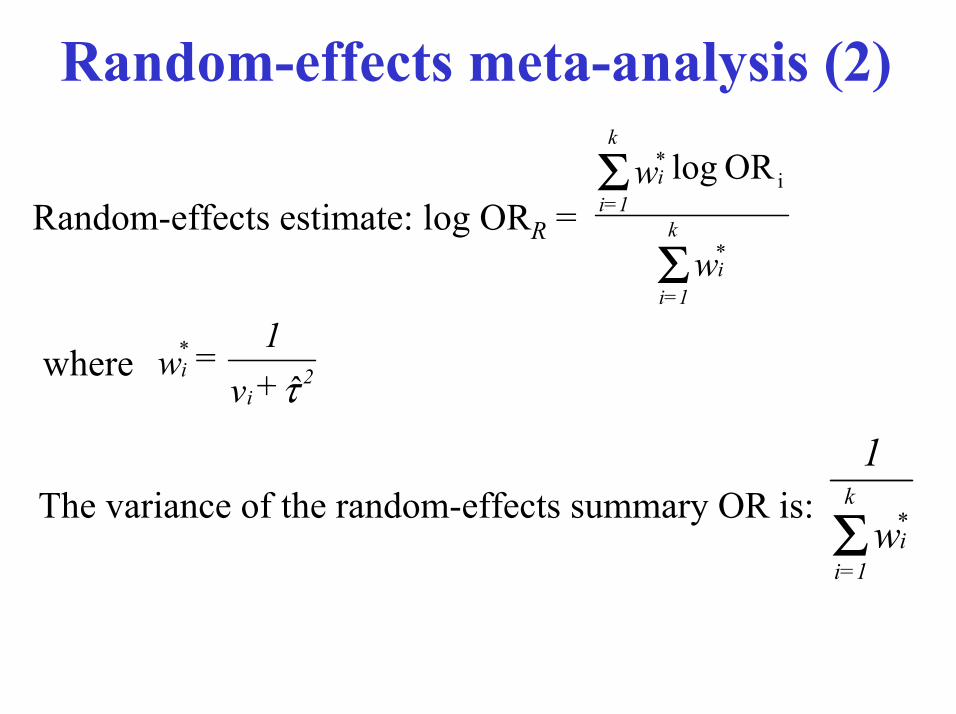
Random-effects meta-analysis (2)

Random-effects estimate: log ORR =w

w

*i

k

=1i

*i

k

=1i

Σ

Σ iOR log

whereτ̂ 2

i

*i +v

1=w

The variance of the random-effects summary OR is:w

1*i

k

=1iΣ

Back to 1996….• Bill Clinton always in the news….• In the UK, Labour look unbeatable….• England’s stars crash out of the European football

championship….• JS gets his first laptop

Stata 5 (1996)• A revolutionary advance, based on the Windows

environment!• Host of new facilities, including……• A new graphics programming command (gph)

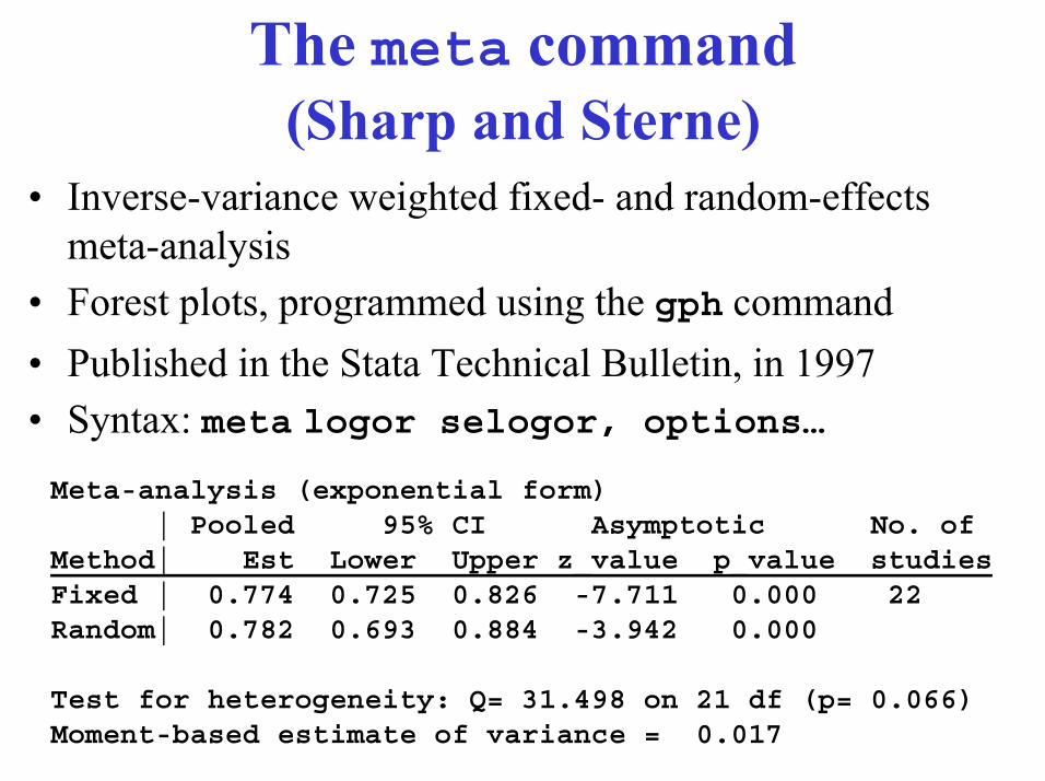
The meta command(Sharp and Sterne)

• Inverse-variance weighted fixed- and random-effects meta-analysis

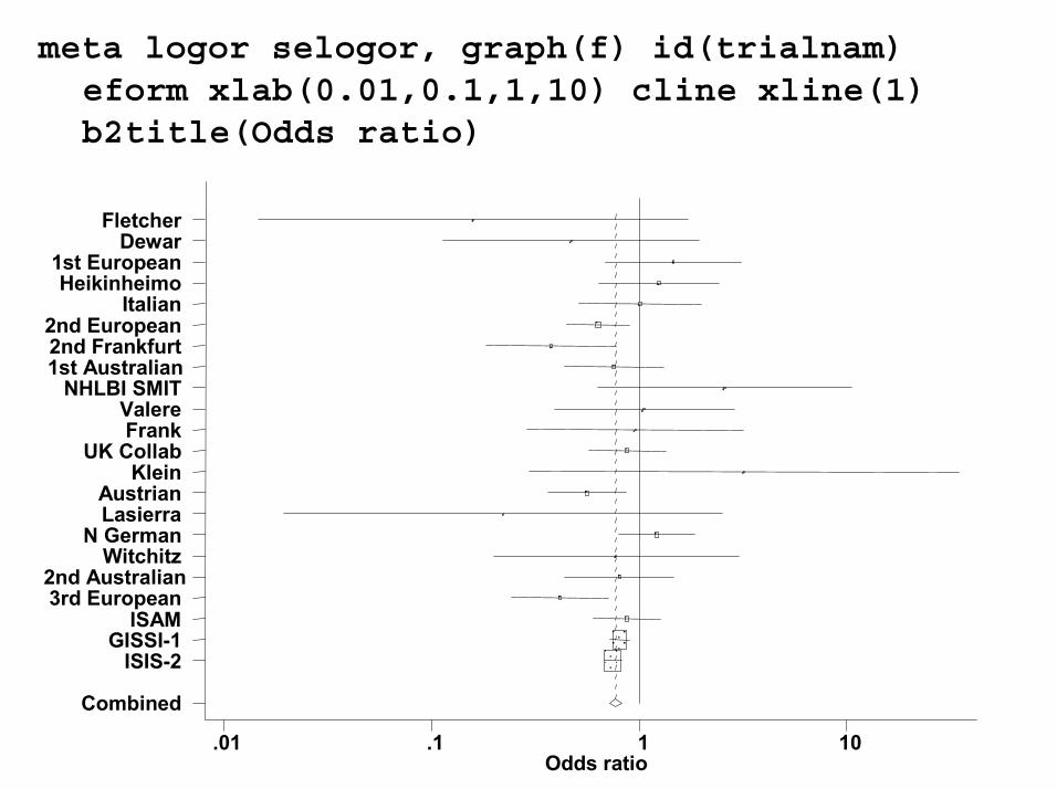
• Forest plots, programmed using the gph command• Published in the Stata Technical Bulletin, in 1997• Syntax: meta logor selogor, options…Meta-analysis (exponential form)

| Pooled 95% CI Asymptotic No. ofMethod| Est Lower Upper z_value p_value studiesFixed | 0.774 0.725 0.826 -7.711 0.000 22Random| 0.782 0.693 0.884 -3.942 0.000

Test for heterogeneity: Q= 31.498 on 21 df (p= 0.066)Moment-based estimate of variance = 0.017

Odds ratio.01 .1 1 10

Combined

ISIS-2GISSI-1

ISAM3rd European2nd Australian

WitchitzN German

LasierraAustrian

KleinUK Collab

FrankValere

NHLBI SMIT1st Australian2nd Frankfurt2nd European

ItalianHeikinheimo

1st EuropeanDewar

Fletcher

meta logor selogor, graph(f) id(trialnam)eform xlab(0.01,0.1,1,10) cline xline(1) b2title(Odds ratio)

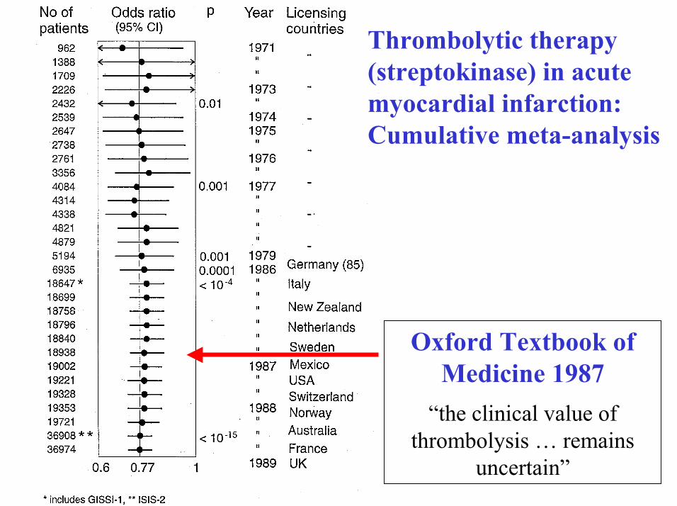
Thrombolytic therapy(streptokinase) in acutemyocardial infarction:Cumulative meta-analysis

Oxford Textbook of Medicine 1987

“the clinical value of thrombolysis … remains

uncertain”

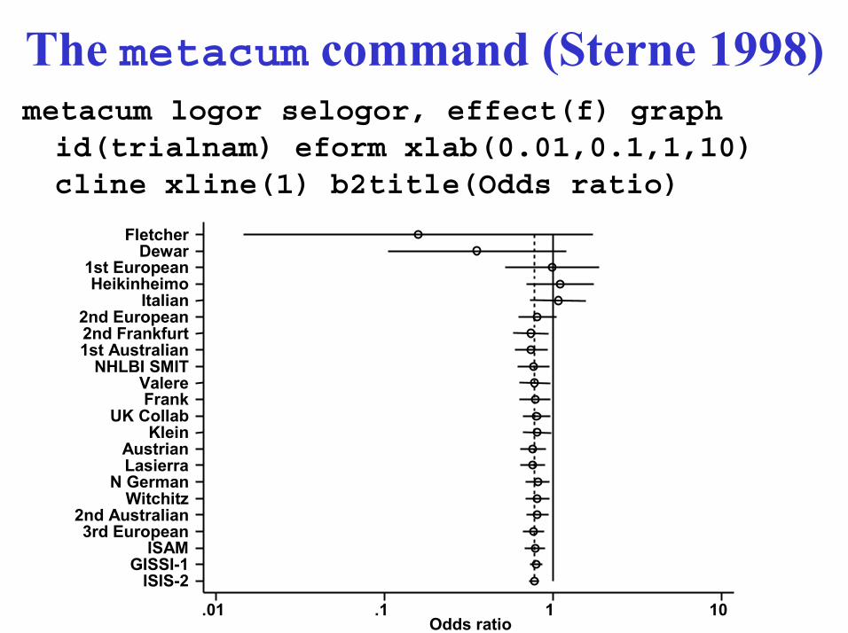
The metacum command (Sterne 1998)metacum logor selogor, effect(f) graph id(trialnam) eform xlab(0.01,0.1,1,10) cline xline(1) b2title(Odds ratio)

Odds ratio.01 .1 1 10

ISIS-2GISSI-1

ISAM3rd European

2nd AustralianWitchitz

N GermanLasierraAustrian

KleinUK Collab

FrankValere

NHLBI SMIT1st Australian2nd Frankfurt2nd European

ItalianHeikinheimo

1st EuropeanDewar

Fletcher

Meanwhile, in Oxford…..• Mike Bradburn, Jon Deeks and Douglas Altman actually

knew something about meta-analysis… • The Cochrane Collaboration was about to release a new

version of its Review manager software, and some checking algorithms were needed

• Mike Bradburn presented a version of his meta command at the 1997 UK Stata Users’ group

“When I found out you’d published your meta command, I sulked for quite a few months, before I could face finishing our command”

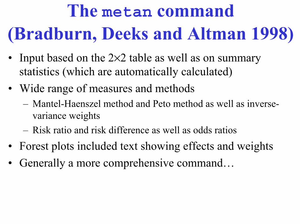
The metan command(Bradburn, Deeks and Altman 1998)• Input based on the 2×2 table as well as on summary

statistics (which are automatically calculated)• Wide range of measures and methods

– Mantel-Haenszel method and Peto method as well as inverse-variance weights

– Risk ratio and risk difference as well as odds ratios

• Forest plots included text showing effects and weights• Generally a more comprehensive command…

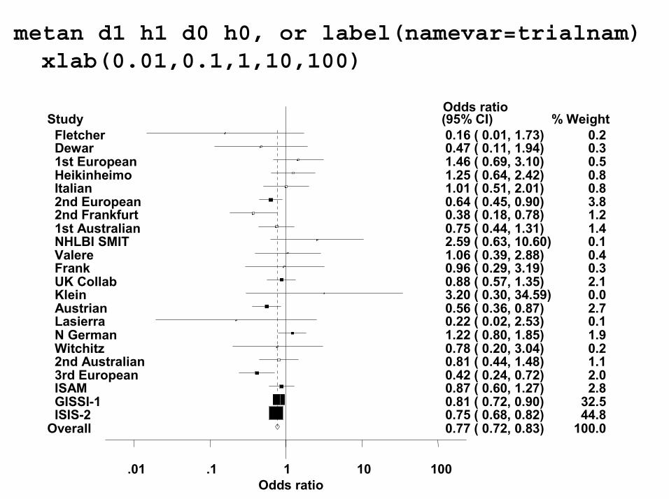
Odds ratio.01 .1 1 10 100

StudyOdds ratio(95% CI) % Weight

Fletcher 0.16 ( 0.01, 1.73) 0.2 Dewar 0.47 ( 0.11, 1.94) 0.3 1st European 1.46 ( 0.69, 3.10) 0.5 Heikinheimo 1.25 ( 0.64, 2.42) 0.8 Italian 1.01 ( 0.51, 2.01) 0.8 2nd European 0.64 ( 0.45, 0.90) 3.8 2nd Frankfurt 0.38 ( 0.18, 0.78) 1.2 1st Australian 0.75 ( 0.44, 1.31) 1.4 NHLBI SMIT 2.59 ( 0.63, 10.60) 0.1 Valere 1.06 ( 0.39, 2.88) 0.4 Frank 0.96 ( 0.29, 3.19) 0.3 UK Collab 0.88 ( 0.57, 1.35) 2.1 Klein 3.20 ( 0.30, 34.59) 0.0 Austrian 0.56 ( 0.36, 0.87) 2.7 Lasierra 0.22 ( 0.02, 2.53) 0.1 N German 1.22 ( 0.80, 1.85) 1.9 Witchitz 0.78 ( 0.20, 3.04) 0.2 2nd Australian 0.81 ( 0.44, 1.48) 1.1 3rd European 0.42 ( 0.24, 0.72) 2.0 ISAM 0.87 ( 0.60, 1.27) 2.8 GISSI-1 0.81 ( 0.72, 0.90) 32.5 ISIS-2 0.75 ( 0.68, 0.82) 44.8

Overall 0.77 ( 0.72, 0.83) 100.0

metan d1 h1 d0 h0, or label(namevar=trialnam) xlab(0.01,0.1,1,10,100)

This week I went through the mails I've received: there’s approximately 200 in the six years I've kept. The users have grown; this year I have had 27 people write, some more than once (that’s >1 a week). The typical mail either asks whether metan can do something or how to use it to analyse data. Early requests tended to be basic "where's the xtick option?" but others have required more time. There were a few bugs too, and so the feedback has helped make metan far better than it was in 1998. People have tended to be appreciative too -one mail this year thanked me for writing it, nothing else.Supporting it is difficult at times: as I work for a cancer charity quite a lot of their time has gone into this. Maybe I shouldn't feel uneasy about that (most requests were from academia), but I do. In my new job I will likely not have the opportunity, save in my own time, to continue this.Given that Stata has gained publicity and users on the back of these routines, it would probably be for the better that Stata’s 1998(?) claim that "Stata should have a meta-analysis command [...] but does not" were carried into practice.

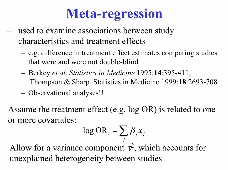
Meta-regression– used to examine associations between study

characteristics and treatment effects– e.g. difference in treatment effect estimates comparing studies

that were and were not double-blind– Berkey et al. Statistics in Medicine 1995;14:395-411,

Thompson & Sharp, Statistics in Medicine 1999;18:2693-708– Observational analyses!!

Assume the treatment effect (e.g. log OR) is related to one or more covariates:

∑=j

jji xβOR log

Allow for a variance component τ2, which accounts for unexplained heterogeneity between studies

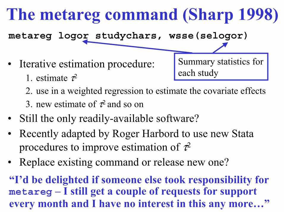
The metareg command (Sharp 1998)

• Iterative estimation procedure:1. estimate τ2

2. use in a weighted regression to estimate the covariate effects3. new estimate of τ2 and so on

• Still the only readily-available software?• Recently adapted by Roger Harbord to use new Stata

procedures to improve estimation of τ2

• Replace existing command or release new one?“I’d be delighted if someone else took responsibility for metareg – I still get a couple of requests for support every month and I have no interest in this any more…”

metareg logor studychars, wsse(selogor)

Summary statistics for each study

Meta-analysis is no panacea...• Contrasting conclusions from

– meta-analyses of the same issue

– meta-analyses and single large trials

• “Low molecular weight heparins seem to have a higher benefit to risk ratio thanunfractionated heparin in preventingperioperative thrombosis”

Leizorovicz A et al. BMJ 1992

• “There is no convincing evidence that in general surgery patients LMWHs, compared with standard heparin, generate a clinically important improvement in the benefit to risk ratio”

Nurmohamed et al. Lancet 1992

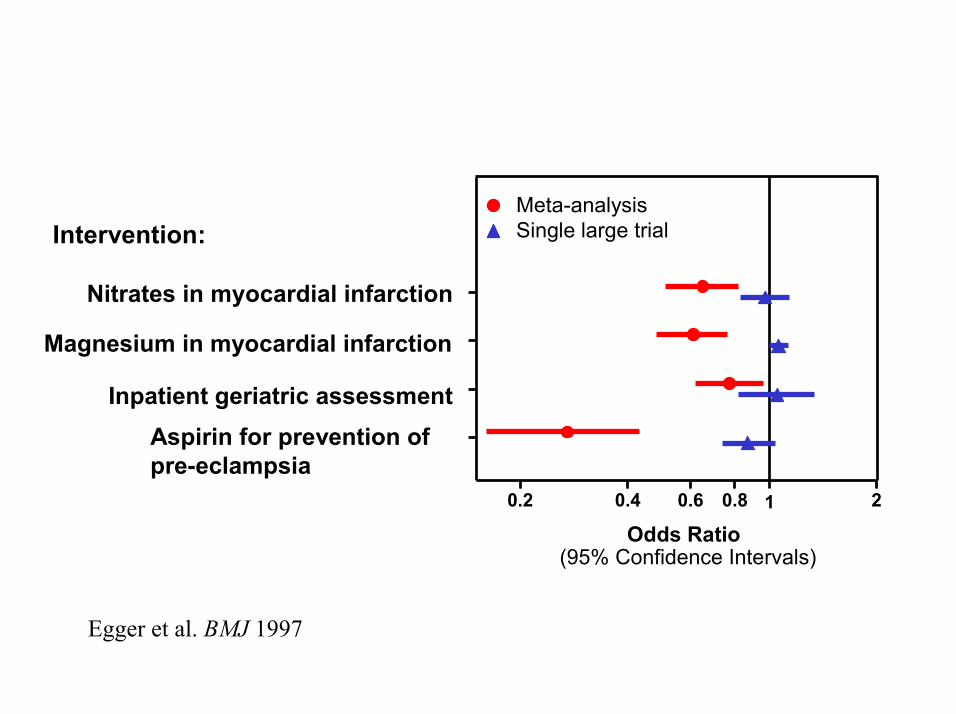
0.2 0.4 0.6 0.8 21

Meta-analysisSingle large trial

Odds Ratio(95% Confidence Intervals)

Nitrates in myocardial infarction

Inpatient geriatric assessment

Magnesium in myocardial infarction

Aspirin for prevention of pre-eclampsia

Intervention:

Egger et al. BMJ 1997

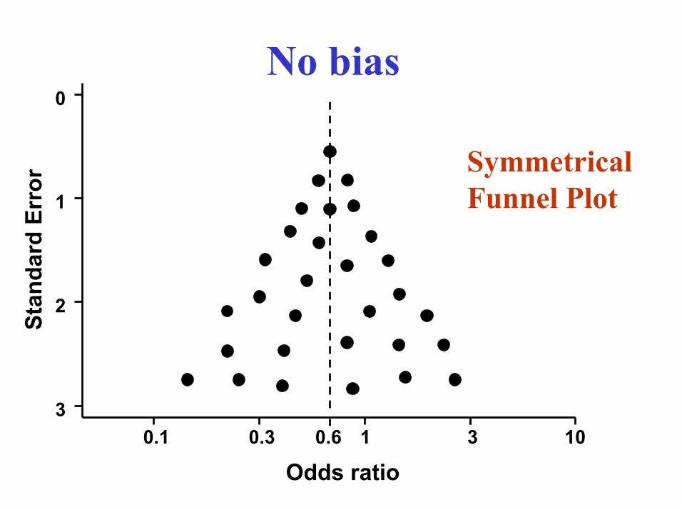
No biasSt

anda

rd E

rror

Odds ratio0.1 0.3 1 3

3

2

1

0

100.6

SymmetricalFunnel Plot

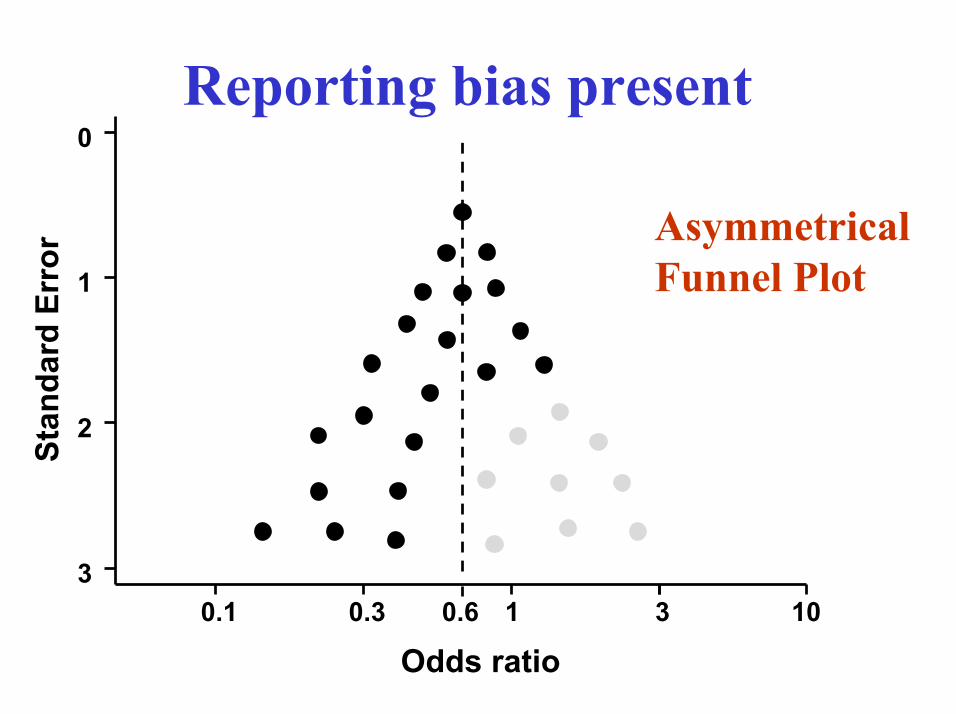
0.1 0.3 1 3 100.6

AsymmetricalFunnel Plot

Reporting bias present

Odds ratio

Stan

dard

Err

or

3

2

1

0

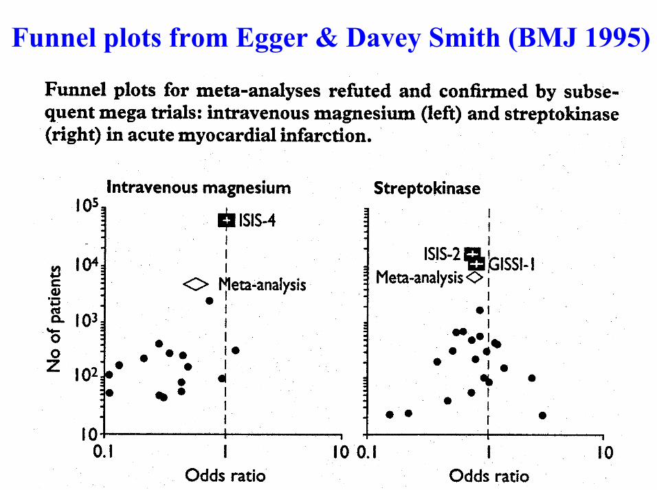
Funnel plots from Egger & Davey Smith (BMJ 1995)

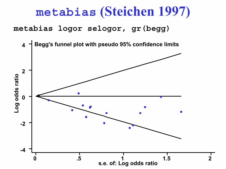
Begg's funnel plot with pseudo 95% confidence limits

Log

odds

ratio

s.e. of: Log odds ratio0 .5 1 1.5 2

-4

-2

0

2

4

metabias logor selogor, gr(begg)

metabias (Steichen 1997)

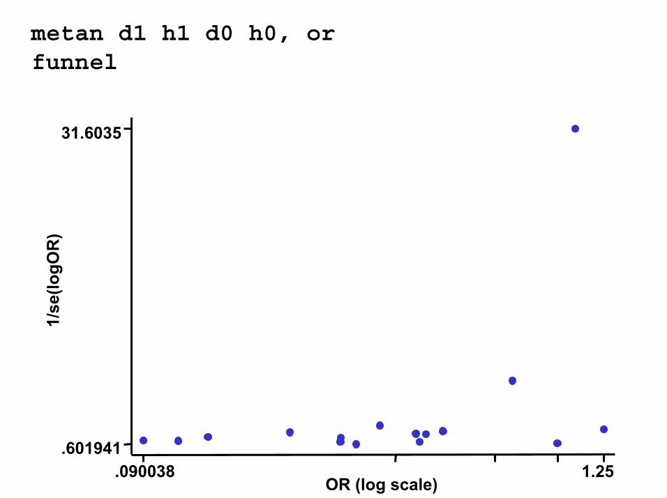
1/se

(logO

R)

OR (log scale).090038 1.25

.601941

31.6035

metan d1 h1 d0 h0, orfunnel

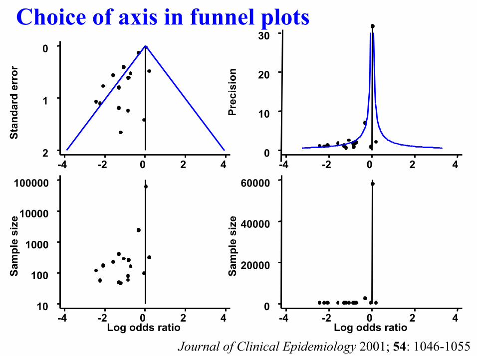
Stan

dard

err

or

-4 -2 0 2 42

1

0

Prec

isio

n

-4 -2 0 2 40

10

20

30

Sam

ple

size

Log odds ratio-4 -2 0 2 4

10

100

1000

10000

100000

Sam

ple

size

Log odds ratio-4 -2 0 2 4

0

20000

40000

60000

Choice of axis in funnel plots

Journal of Clinical Epidemiology 2001; 54: 1046-1055

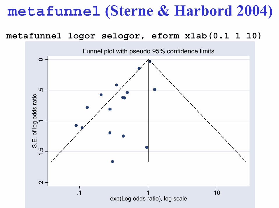
0.5

11.

52

S.E

. of l

og o

dds

ratio

.1 1 10exp(Log odds ratio), log scale

Funnel plot with pseudo 95% confidence limits

metafunnel (Sterne & Harbord 2004)metafunnel logor selogor, eform xlab(0.1 1 10)

Selection models for publication bias

– detect publication bias, based on assuming that a study’s results (e.g. the P value) affect its probability of publication

– Example: assume publication is certain if the study P<0.05. If P>0.05 then publication probability might be a constant (<1) or might decrease with decreasing treatment effect

– More complex models have been proposed, but may require much larger numbers of studies than available in typical meta-analyses

– The complexity of the methods, and the large number of studies needed, probably explain why selection models have not been widely used in practice

Trim and fill(Duval & Tweedie 1999, 2000)

metatrim (Steichen 2000)

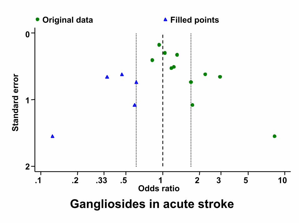
Gangliosides in acute strokeOdds ratio

Original data

.1 .2 .33 .5 1 2 3 5 10

Stan

dard

err

or

2

1

0

Filled points

Selection models are unlikely to account (fully) for funnel plot asymmetry

• Statistically significant studies are more likely to produce multiple publications

• Large studies are more likely to be published whatever their results

• Poorer quality studies produce more extreme treatment effects, and are also more likely to be small

• The true treatment effect may differ according to study size:– Intensity of intervention– Differences in underlying risk

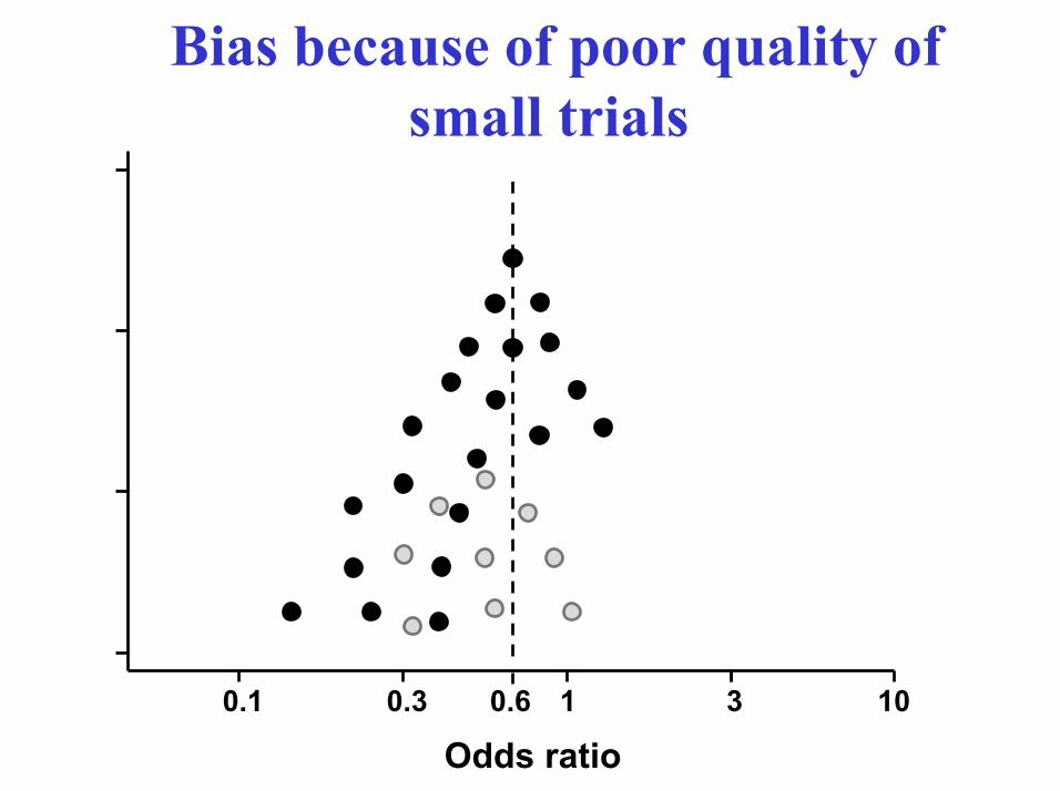
0.1 0.3 1 3 100.6

Bias because of poor quality of small trials

Odds ratio

Small study effect

- a tendency for smaller trials in ameta-analysis to show greater treatmenteffects than the larger trials

Small study effects need not result from bias

Statistical tests for funnel plot asymmetry

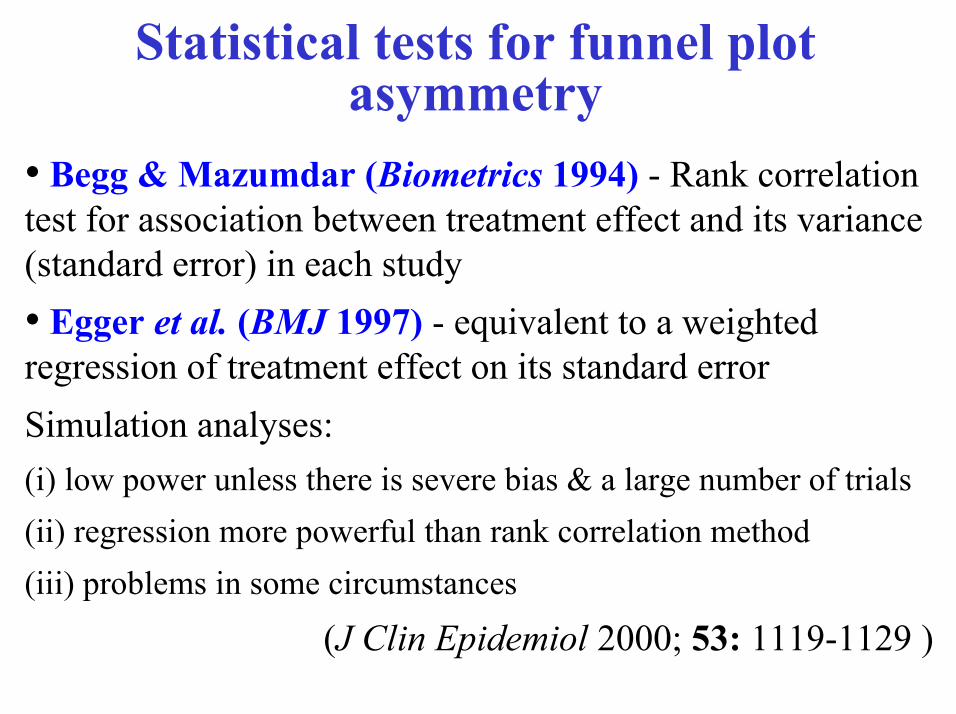
• Begg & Mazumdar (Biometrics 1994) - Rank correlation test for association between treatment effect and its variance (standard error) in each study• Egger et al. (BMJ 1997) - equivalent to a weighted regression of treatment effect on its standard errorSimulation analyses: (i) low power unless there is severe bias & a large number of trials(ii) regression more powerful than rank correlation method (iii) problems in some circumstances

(J Clin Epidemiol 2000; 53: 1119-1129 )

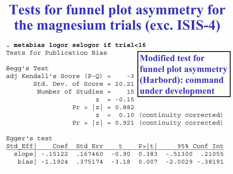
Tests for funnel plot asymmetry for the magnesium trials (exc. ISIS-4)

. metabias logor selogor if trial<16Tests for Publication Bias

Begg's Testadj Kendall's Score (P-Q) = -3

Std. Dev. of Score = 20.21 Number of Studies = 15

z = -0.15Pr > |z| = 0.882

z = 0.10 (continuity corrected)Pr > |z| = 0.921 (continuity corrected)

Egger's testStd_Eff| Coef Std Err t P>|t| 95% Conf Intslope| -.15122 .167460 -0.90 0.383 -.51300 .21055bias| -1.1924 .375174 -3.18 0.007 -2.0029 -.38191

Modified test for funnel plot asymmetry (Harbord): command under development

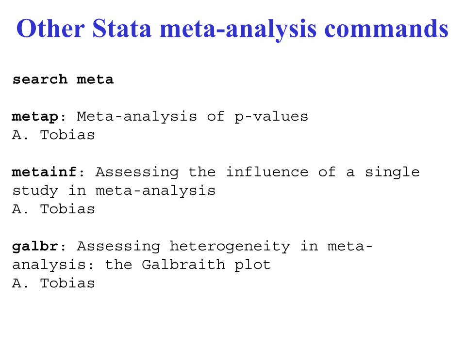
Other Stata meta-analysis commands

search meta

metap: Meta-analysis of p-valuesA. Tobias

metainf: Assessing the influence of a single study in meta-analysisA. Tobias

galbr: Assessing heterogeneity in meta-analysis: the Galbraith plotA. Tobias

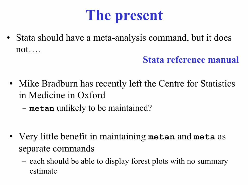
The present• Stata should have a meta-analysis command, but it does

not….Stata reference manual

• Mike Bradburn has recently left the Centre for Statistics in Medicine in Oxford– metan unlikely to be maintained?

• Very little benefit in maintaining metan and meta as separate commands– each should be able to display forest plots with no summary

estimate

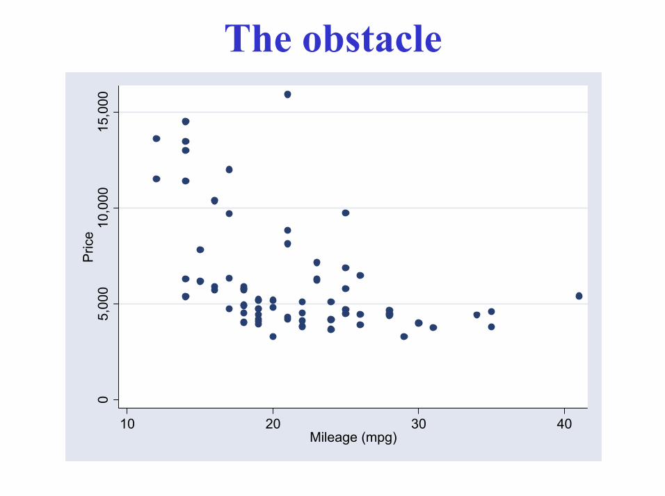
The obstacle0

5,00

010

,000

15,0

00P

rice

10 20 30 40Mileage (mpg)

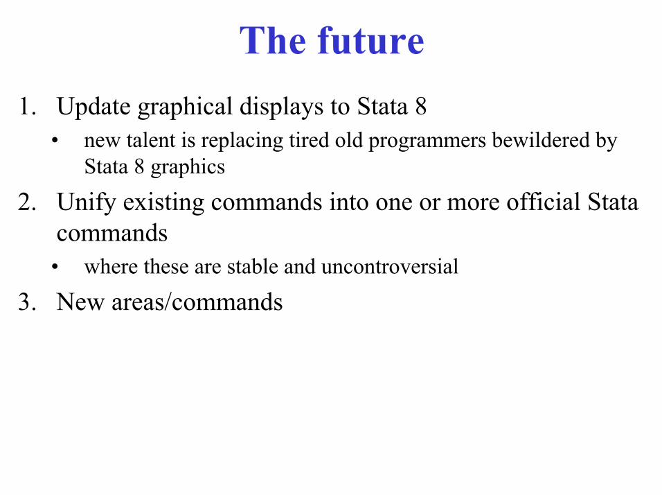
The future1. Update graphical displays to Stata 8

• new talent is replacing tired old programmers bewildered by Stata 8 graphics

2. Unify existing commands into one or more official Stata commands• where these are stable and uncontroversial

3. New areas/commands

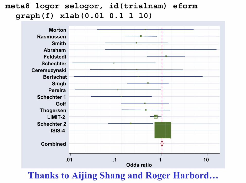
Combined

ISIS-4Schechter 2

LIMIT-2Thogersen

GolfSchechter 1

PereiraSingh

BertschatCeremuzynski

SchechterFeldstedtAbraham

SmithRasmussen

Morton

.01 .1 1 10

meta8 logor selogor, id(trialnam) eformgraph(f) xlab(0.01 0.1 1 10)

Odds ratio

Thanks to Aijing Shang and Roger Harbord…

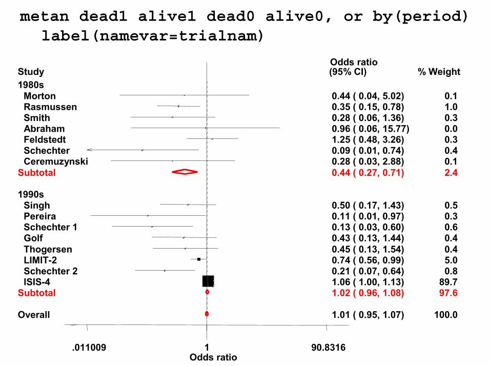
Odds ratio.011009 1 90.8316

StudyOdds ratio(95% CI) % Weight

1980sMorton 0.44 ( 0.04, 5.02) 0.1 Rasmussen 0.35 ( 0.15, 0.78) 1.0 Smith 0.28 ( 0.06, 1.36) 0.3 Abraham 0.96 ( 0.06, 15.77) 0.0 Feldstedt 1.25 ( 0.48, 3.26) 0.3 Schechter 0.09 ( 0.01, 0.74) 0.4 Ceremuzynski 0.28 ( 0.03, 2.88) 0.1

Subtotal 0.44 ( 0.27, 0.71) 2.4

1990sSingh 0.50 ( 0.17, 1.43) 0.5 Pereira 0.11 ( 0.01, 0.97) 0.3 Schechter 1 0.13 ( 0.03, 0.60) 0.6 Golf 0.43 ( 0.13, 1.44) 0.4 Thogersen 0.45 ( 0.13, 1.54) 0.4 LIMIT-2 0.74 ( 0.56, 0.99) 5.0 Schechter 2 0.21 ( 0.07, 0.64) 0.8 ISIS-4 1.06 ( 1.00, 1.13) 89.7

Subtotal 1.02 ( 0.96, 1.08) 97.6

Overall 1.01 ( 0.95, 1.07) 100.0

metan dead1 alive1 dead0 alive0, or by(period) label(namevar=trialnam)

New developments• Meta-analysis of diagnostic tests

– Major area of expansion for the Cochrane Collaboration– Statistically, much more complex than meta-analysis of

randomised controlled trials– First command (meta_lr) recently released by Aijing Shang– Formal synthesis of these studies requires bivariate methods

accounting for the association between sensitivity and specificity (meta-analyse in ROC-space)

– Obvious extensions to existing ROC methods in Stata– Opportunities to use gllamm and new mixed models

procedures to be released in Stata 9?

• As always, developments will occur in areas that no-one predicts…

Thanks to…

• Stephen Sharp• Matthias Egger• Tom Steichen• Mike Bradburn• Roger Harbord• Aijing Shang