Measuring brain connectivity: Diffusion tensor imaging validates resting state temporal correlations

NeuroImage 43 (2008) 554–561

Contents lists available at ScienceDirect

NeuroImage

j ourna l homepage: www.e lsev ie r.com/ locate /yn img

Measuring brain connectivity: Diffusion tensor imaging validates resting statetemporal correlations

Pawel Skudlarski a,b,⁎, Kanchana Jagannathan a, Vince D. Calhoun a,b,c,d, Michelle Hampson e,Beata A. Skudlarska f, Godfrey Pearlson a,b

a Olin Neuropsychiatry Research Center, Institute of Living, Hartford Hospital, Hartford, 06106 CT, USAb Department of Psychiatry, Yale University School of Medicine, New Haven, 06510 CT, USAc The MIND Institute, Albuquerque, 87131 NM, USAd Department of Electrical and Computer Engineering, University of New Mexico, Albuquerque, 87131 NM, USAe Department of Diagnostic Radiology, Yale University School of Medicine, New Haven, 06510 CT, USAf Bridgeport Hospital, Center for Geriatrics, Bridgeport, 06610 CT, USA

⁎ Corresponding author. Olin Neuropsychiatry ReseaInstitute of Living, Whitehall Bldg., 200 Retreat Ave. Ha860 545 7797.

E-mail address: [email protected] (P. Skudl

1053-8119/$ – see front matter © 2008 Elsevier Inc. Alldoi:10.1016/j.neuroimage.2008.07.063

a b s t r a c t

Article history:

TI) and resting state temporal correlations (RSTC) are two leading techniques forinvestigating the connectivity of the human brain. They have been widely used to investigate the strength ofanatomical and functional connections between distant brain regions in healthy subjects, and in clinicalpopulations. Though they are both based on magnetic resonance imaging (MRI) they have not yet beencompared directly. In this work both techniques were employed to create global connectivity matricescovering the whole brain gray matter. This allowed for direct comparisons between functional connectivitymeasured by RSTC with anatomical connectivity quantified using DTI tractography. We found thatconnectivity matrices obtained using both techniques showed significant agreement. Connectivity mapscreated for a priori defined anatomical regions showed significant correlation, and furthermore agreementwas especially high in regions showing strong overall connectivity, such as those belonging to the defaultmode network. Direct comparison between functional RSTC and anatomical DTI connectivity, presented herefor the first time, links two powerful approaches for investigating brain connectivity and shows their strongagreement. It provides a crucial multi-modal validation for resting state correlations as representingneuronal connectivity. The combination of both techniques presented here allows for further combiningthem to provide richer representation of brain connectivity both in the healthy brain and in clinicalconditions.

© 2008 Elsevier Inc. All rights reserved.

Introduction

Resting state temporal correlations (RSTC) between fMRI timecourses of distant brain regions were first observed (Biswal et al.,1995) between contralateral motor cortices and later between otherregions known to be strongly functionally connected, such as auditoryand visual areas (Lowe et al., 2000) and language regions (Hampson etal., 2002). The recognition of the importance of the default modenetwork (DMN) (Greicius et al., 2003) and its anti-correlatedcounterpart the task positive network increased interest in restingcorrelations as a tool for defining functional systems in the workinghuman brain. Not only are RSTC useful to improve the basicunderstanding of the healthy working brain, but their modifications,e.g. in the DMN are found in several clinical conditions (Andrews-

rch Center, Hartford Hospital,rtford, CT 06106, USA. Fax: +1

arski).

rights reserved.

Hanna et al., 2007; Bluhm et al., 2007; Cherkassky et al., 2006;Greicius et al., 2004; Rombouts et al., 2005; Sorg et al., 2007; Garrity etal., 2007). Converging indirect evidence for the neuronal origin ofresting state correlations in the fMRI time courses has come fromstudies of physiology of MRI signal such as (Biswal et al., 1997; Birn etal., 2006; Shmueli et al., 2007) on awake and anesthetized humans(Kiviniemi et al., 2005); (Peltier et al., 2005) as well as monkeys(Takahashi et al., 2007) and are best reviewed in De Luca et al. (2006);Fox and Raichle (2007). The basic physiological mechanism is still notwell understood and the interpretation of changes of its intensity asrepresenting modification of neural connections and informationflow between brain regions remains uncertain. If, as is widelybelieved, the RSTC represents important information on neuronalconnectivity between distant brain regions, these regions must useneuronal connections to carry the associated information flow. Toallow for such communication between nodes of brain networksthere must be a white matter fiber path connecting them. Thispathway does not have to be direct, but nevertheless one expectsthat functional connectivity must in some manner be dependent on

555P. Skudlarski et al. / NeuroImage 43 (2008) 554–561

the strength of the relevant anatomical neuronal connection. It istherefore important to investigate similarities between connectivitymeasures obtained from the analysis of RSTC and anatomicalmeasures of strength of neuronal connectivity.

In this paper we compare the strength of anatomical andfunctional connectivity. We expected that the connectivity measuresobtained using resting correlations would be consistent with thoseobtained independently using diffusion tensor imaging (DTI). Suchagreement would support the hypothesis that RSTC measures inter-regional connectivity.

Both DTI and temporal correlations in resting state fMRI offer thepotential to investigate the neuronal connectivity of the workinghuman brain. DTI measures the integrity of white matter tracts, whileRSTC examines the similarities between spontaneous fluctuations thatoccur over time in distal gray matter areas. Both techniques use MRIscanning, but are independent, use different imaging sequences andemploy different physical principles and physiological effects. Becausethose two techniques measure different aspects of neuronal con-nectivity, much can be learned by comparing howwell they agree andwhere and why they differ.

Diffusion tensor imaging is based on analysis of the inhomo-geneity of water diffusion. Multiple MRI images are taken thatmeasure the ability of water to diffuse along different gradientdirections. These measurements allow calculation of the diffusiontensor used to measure local anisotropy (usually expressed asfractional anisotropy, FA) that can be understood as representingthe local “strength” of white matter nerve bundles. This tensor canbe also used find the dominant direction of diffusion and thus totrack white matter tracts in DTI tractography (Hagmann et al., 2003);(Le Bihan et al., 2001). DTI is widely used to investigate white matterfiber connectivity and thus the anatomical structure of distant brainconnections. While local anisotropy measures are successfully usedquantitatively, fiber tracking is most often used in a qualitative,descriptive manner. The quantification is performed successfully(Nucifora et al., 2007); (Mueller et al., 2007) for specified whitematter tracts but has not been employed in a global approach toinvestigate whole brain connectivity.

RSTC is now often used to quantify the strength of brainconnectivity, yet little is understood about why and how suchcorrelations represent the actual strength of neuronal connectivitybetween any given regions. While the presence of connectingneuronal fibers (anatomical connectivity) is necessary for regions tointeract, the strength of functional connectivity can presumably bemodulated in various mental states and does not have to be directlyrelated to anatomical strength of fiber bundles that can be observedvia DTI. For example the first and most prominent connectionsobserved with resting state correlations were those connecting leftand right motor cortex, and those regions are connected by directwhite matter fibers.

The need to combine anatomical and functional connectivity hasbeen recognized e.g. in Fox and Raichle (2007), the excellent review ofcurrent work is found in the review (Gordon et al., 2007). The relatedwork (Koch et al., 2002) was limited to neighboring gyri and foundonly weak trends towards agreement between techniques; so far noone has been able to compare them globally.

This paper presents a novel approach in which we use DTItractography to estimate the strength of anatomical connection forany two voxels in the brain. We show how both techniques can beused to create a global gray matter connectivity matrix that providesa quantitative measure of connectivity strength for any two graymatter voxels in standard brain space. Such matrices can becompared spatially within subjects to compute how well theyagree for any given subject or in comparison between averagecompositemaps. The comparison can be alsomade between subjects,any pair of voxels or of regions can be analyzed across a subjectpopulation.

The agreement between both measures provides an importantcross validation, as both techniques are still being developed andneither has been well established as a working tool for neuroscience.Having established the overall omnibus agreement between them, thelocal or population differences between connectivity measures canprovide insights into a specific connectivity deficit, to characterize it asrelated to anatomical circuit disruption or to functional impairment ofneuronal connectivity caused e.g. by neurotransmitter imbalances,failure of specific brain regions to activate, etc.

Methods

Subjects

Data was collected from 41 carefully screened healthy individualsaged 28±10 years, 23male, whowere participating as normal controlsin various cognitive experiments approved by the Hartford HospitalIRB. Subjects were free of psychiatric disorders, as assessed by theSCID (Williams et al., 1992), were neurologically normal, not substanceabusers and had signed informed consents.

Imaging

MR imaging was performed using a 3 T Siemens Allegra scanner(Siemens, Erlangen, Germany). T1 structural images were collected foranatomical coregistration and segmentation. Resting state data werecollected during one run of 210 images at TR/TE 1500/28 ms, flip angle65°, FOV 24×24 cm, 64×64 matrix, 3 by 3 mm in plane resolution;5 mm slice thickness, 30 slices. DTI was performed using a twice-refocused spin echo (Tuch et al., 2003); TR/TE=5800/87 ms,FOV=20 cm, acquisition and reconstruction matrices=128×96 and128×128, 8 averages, diffusion sensitizing orientations in 12 direc-tions with one b0, b=1000 s/mm2, 45 contiguous axial slices with3 mm section thickness. Data processing was performed using SPM2(Friston et al., 1999), DtiStudio (Johns Hopkins University, Baltimore,MD; http://cmrm.med.jhmi.edu) (for fiber tracking) and in-housesoftware written using MATLAB.

Brain segmentation

StandardSPM2segmentation toolwasused to segmenteachsubject'sbrain into three components representing graymatter, whitematter andcerebrospinal fluid (CSF). Individualmaskswere converted into standardspace with 4×4×4 mm resolution and the composite masks werecreated for white and gray matter, each covering top 5000 voxels thatwere found most consistently in individual brain segmentations.

Resting state data analysis

The preprocessing of the resting state data generally followed thatof Margulies et al. (2007), Fox et al. (2005). The first 5 images weredropped, data were motion corrected using SPM2, the remaining datawere band-pass filtered to remove signal of frequencies higher than0.1 Hz (non-BOLD signal, mostly cardiac and respiratory noise) andfrequencies lower than 0.005 Hz (mostly signal drift due to scannerinstabilities). The data were intensity normalized for each slice (e.a.the intensity of each slice image was divided by its mean), motioncorrected and spatially normalized to a standard template using SPM2. Images were smoothed using a Gaussian filter of FWHM 4 mm andresampled to a resolution of 4 mm3. Brain segmentation of the T1 datawas performed for each subject using SPM2 tool and brainwas dividedinto 3 components of white and gray matter and CFS. The correlationbetween time courses was calculated for all 5000×5000 voxel pairswithin gray matter. The correlation was estimated using a GLMmodelthat removed 6 motion estimates. The final resting correlation mapwas transformed to a Z-distribution using Fisher's transform. The

Table 1The anatomically defined regions with Talairach coordinates of its center and sizes

ROI name X Y Z Size (mm3)

Angular L −46 −62 36 1040Angular R 45 −60 37 1168CingAnt 0 31 17 1376CingPost 0 −47 33 480Cingulate 0 −22 45 1248Cuneus 5 −77 26 1216IFG L −45 22 12 1976IFG R 45 22 12 1864IPL L −52 −43 39 1032IPL R 50 −42 38 760Insula L −40 −5 3 1568Insula R 40 −7 4 1648Lingual G. 5 −70 −1 1032Middle FG L −35 33 31 2496Middle FG R 34 31 32 2256Med. Occ FG L −44 −76 4 832Med. Occ FG R 44 −77 4 832Middle TG L −53 −47 5 1976Middle TG R 53 −50 6 1624Medial FG −1 34 28 3168Postcentral L −54 −25 36 1104Postcentral R 54 −26 35 672Precuneus 2 −62 50 1168Sup. Temp G L −54 −22 8 656Sup. Temp G R 54 −20 8 664Thalamus 0 −21 5 592

556 P. Skudlarski et al. / NeuroImage 43 (2008) 554–561

distribution was fitted to a Gaussian and adjusted to a zero-centerednormal distribution as in Lowe et al. (2002); Hampson et al. (2004).

Diffusion tensor imaging data analysis

Tractography was performed using DTIstudio software package.Fiber tracts were detected using standard FACT algorithm with stopcriteria of FAN0.25 and turning angle of 70°. On average 40,000 fiberswere detected for a single subject. After calculating fiber tracts, thefiber coordinates were normalized into standard space. Using SPM2, anonlinear transformation was computed between the B0 image andthe provided Montreal Neurologic Institute T2 template and thetransformation was applied to each fiber coordinate.

While fiber tracking was performed in whole brain, the calculationof DTI connectivity matrix was limited to white matter only. Whitematter was defined by mask created for each study using standardSPM2 segmentation algorithm. To quantify the strength of anatomicalconnectivity between any two white matter voxels, we counted alltracts connecting them identified during the tractography step. Thiscreated a first order matrix of direct connectivity. Multiplying thismatrix by itself creates a second matrix that counts all possible pathsthat can be built using two connected tracts. Further multiplicationsyields matrices counting any longer paths. The final outcome wascalculated by summing the number of paths of each length (up to 8segments) with a weighting that heavily penalized more indirectpaths. The connectivity measure CDTI(x,y), for any given voxel pair wasthen defined as the sum of contributions from all path lengths:

CDTI x; yð Þ ¼ ∑i¼1:N2^ −Nð Þ log 1þ CN x; yð Þð Þ;

where CN is number of paths of length connecting voxels x and y.The inclusion of paths of various lengths had a twofold purpose. It

allowed for the possibility of multisynaptic connections and alsoprovided a statistical remedy for the problem of fibers crossing and ortouching. If fibers are crossed or are closer than image resolution, thefiber tracking algorithmmay stop (if crossed fibers cause the fractionalanisotropy to be higher than set threshold), or can lead to trackingalong the wrong fiber. Even if only one of possible fibers is detected ina region of crossing, the other will be included as higher order pathsbuilt of all fibers reaching the point of crossing. The weighting causesconnectivity measures for voxels that can be connected by a path ofany length to be significantly larger that those that require highernumber of segments. This lowers the possibility of false positives, asthe connections that are composed of large number of segments thatare more likely be artifactual are given a low connectivity value. Theirinclusion does not change the status of more direct fibers as mostlyconnected but it expands the area in the connectivity space that isestimated. Even with as many as eight fibers allowed to form a path,only between 30% and 70% of voxels pairs are assigned a non-zeroconnectivity estimate.

The weighting factors that heavily favor the direct connections areworking to ensure that the multi-path procedure allows estimation ofconnectivity for each voxel pair that is not connected by a direct path,but its connectivity estimate is substantially lower that those of voxelsconnected by more direct path. We have checked that changing thelength of path to a smaller value does not change the main results ofthis paper. Even if only direct fiber path are included the maincorrelation between DTI and functional connectivity maps remainshighly significant and while connectivity maps show less voxels, theregions shown as most strongly connected in the multi-path mapspresented here are still shown as the main connected regions.

White matter–gray matter transition

An important problem in comparing the two methods here is thatthey are focused on different tissues; DTI fiber tracking estimates

nerve fiber location by analysis of constraints to water diffusionoccurring in white matter, while resting correlation between fMRItime courses is based on BOLD effects observed in gray matter. Toresolve this problem we incorporated brain segmentation usingstandard SPM tools. We estimated DTI connectivity only for whitematter and resting state only for gray matter. Given the final goal ofestimating the strength of connectivity between cortical gray matterareas, we had to calculate the DTI connectivity for any given pair ofgray matter voxels. The gray matter connectivity matrix for DTI wascalculated from the white matter connectivity matrix as follows. Foreach gray matter voxel we have defined the neighborhood of closestwhite matter voxels. To define the size of this neighborhood for anygiven gray matter voxel, we found the nearest white matter voxel. Thedistance to this voxel was then increased by one voxel size (4 mm) tocreate the neighborhood radius size (defined separately for each graymatter voxel). The white matter neighborhood was defined by allwhite matter within this radius. On average, this neighborhood had aradius of 12 mm and consisted of 5 white matter voxels. In some casesthis led to inclusion of white matter voxels that were somewhatdistant to our target gray matter voxel, but the rule was based on thepremise that even gray matter voxels embedded far from the nearestwhite matter fibers have to gather input from some most proximatewhite matter fibers.

The resulting DTI connectivity matrix has a non-Gaussiandistribution; it was positively skewed and had a high (25–75%)proportion of zeros. We did not estimate the significance of individualDTI maps, the significance of all presented results was estimated usingthe between-subject variance.

Geometrical distance correction

Both techniques outlined above tend to break down for proximatevoxels. Resting correlations are elevated due to scanner-introducedcorrelations between nearest neighbors, interpolations and spatialsmoothing. DTI based connectivity for gray matter relies on findingnearest white matter neighbors that were found on average 7 mmapart. For this reason we excluded all voxel pairs located closer than24 mm from the analysis. Even for larger distances, both measuresdecreased with increasing distance and thus show strong negative

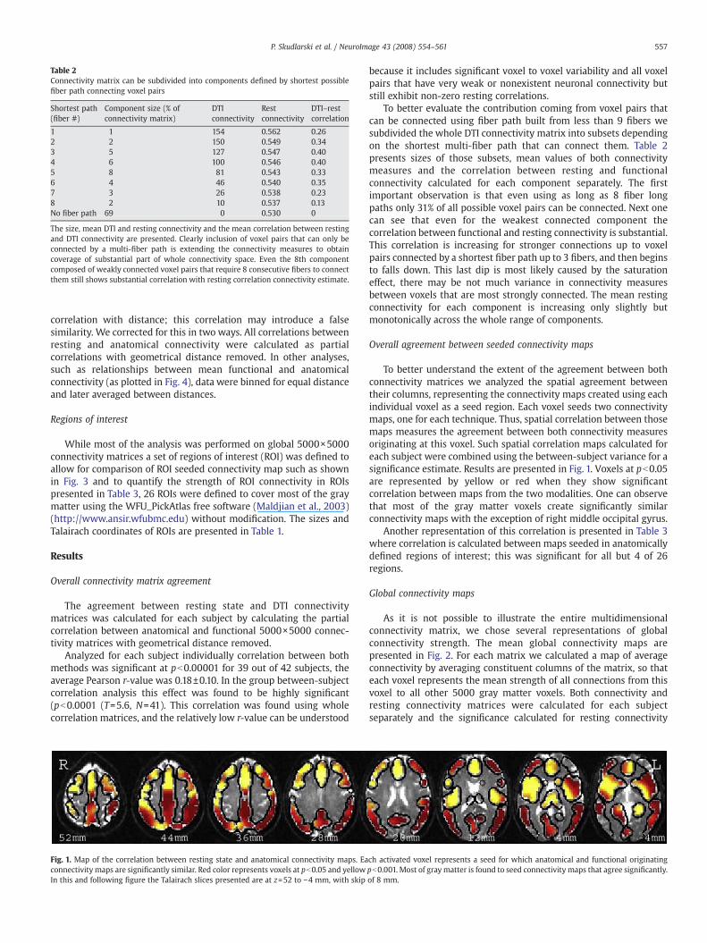
Table 2Connectivity matrix can be subdivided into components defined by shortest possiblefiber path connecting voxel pairs

Shortest path(fiber #)

Component size (% ofconnectivity matrix)

DTIconnectivity

Restconnectivity

DTI–restcorrelation

1 1 154 0.562 0.262 2 150 0.549 0.343 5 127 0.547 0.404 6 100 0.546 0.405 8 81 0.543 0.336 4 46 0.540 0.357 3 26 0.538 0.238 2 10 0.537 0.13No fiber path 69 0 0.530 0

The size, mean DTI and resting connectivity and the mean correlation between restingand DTI connectivity are presented. Clearly inclusion of voxel pairs that can only beconnected by a multi-fiber path is extending the connectivity measures to obtaincoverage of substantial part of whole connectivity space. Even the 8th componentcomposed of weakly connected voxel pairs that require 8 consecutive fibers to connectthem still shows substantial correlation with resting correlation connectivity estimate.

557P. Skudlarski et al. / NeuroImage 43 (2008) 554–561

correlation with distance; this correlation may introduce a falsesimilarity. We corrected for this in two ways. All correlations betweenresting and anatomical connectivity were calculated as partialcorrelations with geometrical distance removed. In other analyses,such as relationships between mean functional and anatomicalconnectivity (as plotted in Fig. 4), data were binned for equal distanceand later averaged between distances.

Regions of interest

While most of the analysis was performed on global 5000×5000connectivity matrices a set of regions of interest (ROI) was defined toallow for comparison of ROI seeded connectivity map such as shownin Fig. 3 and to quantify the strength of ROI connectivity in ROIspresented in Table 3, 26 ROIs were defined to cover most of the graymatter using the WFU_PickAtlas free software (Maldjian et al., 2003)(http://www.ansir.wfubmc.edu) without modification. The sizes andTalairach coordinates of ROIs are presented in Table 1.

Results

Overall connectivity matrix agreement

The agreement between resting state and DTI connectivitymatrices was calculated for each subject by calculating the partialcorrelation between anatomical and functional 5000×5000 connec-tivity matrices with geometrical distance removed.

Analyzed for each subject individually correlation between bothmethods was significant at pb0.00001 for 39 out of 42 subjects, theaverage Pearson r-value was 0.18±0.10. In the group between-subjectcorrelation analysis this effect was found to be highly significant(pb0.0001 (T=5.6, N=41). This correlation was found using wholecorrelation matrices, and the relatively low r-value can be understood

Fig. 1. Map of the correlation between resting state and anatomical connectivity maps. Eaconnectivity maps are significantly similar. Red color represents voxels at pb0.05 and yellowIn this and following figure the Talairach slices presented are at z=52 to −4 mm, with skip

because it includes significant voxel to voxel variability and all voxelpairs that have very weak or nonexistent neuronal connectivity butstill exhibit non-zero resting correlations.

To better evaluate the contribution coming from voxel pairs thatcan be connected using fiber path built from less than 9 fibers wesubdivided the whole DTI connectivity matrix into subsets dependingon the shortest multi-fiber path that can connect them. Table 2presents sizes of those subsets, mean values of both connectivitymeasures and the correlation between resting and functionalconnectivity calculated for each component separately. The firstimportant observation is that even using as long as 8 fiber longpaths only 31% of all possible voxel pairs can be connected. Next onecan see that even for the weakest connected component thecorrelation between functional and resting connectivity is substantial.This correlation is increasing for stronger connections up to voxelpairs connected by a shortest fiber path up to 3 fibers, and then beginsto falls down. This last dip is most likely caused by the saturationeffect, there may be not much variance in connectivity measuresbetween voxels that are most strongly connected. The mean restingconnectivity for each component is increasing only slightly butmonotonically across the whole range of components.

Overall agreement between seeded connectivity maps

To better understand the extent of the agreement between bothconnectivity matrices we analyzed the spatial agreement betweentheir columns, representing the connectivity maps created using eachindividual voxel as a seed region. Each voxel seeds two connectivitymaps, one for each technique. Thus, spatial correlation between thosemaps measures the agreement between both connectivity measuresoriginating at this voxel. Such spatial correlation maps calculated foreach subject were combined using the between-subject variance for asignificance estimate. Results are presented in Fig. 1. Voxels at pb0.05are represented by yellow or red when they show significantcorrelation between maps from the two modalities. One can observethat most of the gray matter voxels create significantly similarconnectivity maps with the exception of right middle occipital gyrus.

Another representation of this correlation is presented in Table 3where correlation is calculated between maps seeded in anatomicallydefined regions of interest; this was significant for all but 4 of 26regions.

Global connectivity maps

As it is not possible to illustrate the entire multidimensionalconnectivity matrix, we chose several representations of globalconnectivity strength. The mean global connectivity maps arepresented in Fig. 2. For each matrix we calculated a map of averageconnectivity by averaging constituent columns of the matrix, so thateach voxel represents the mean strength of all connections from thisvoxel to all other 5000 gray matter voxels. Both connectivity andresting connectivity matrices were calculated for each subjectseparately and the significance calculated for resting connectivity

ch activated voxel represents a seed for which anatomical and functional originatingpb0.001. Most of gray matter is found to seed connectivity maps that agree significantly.of 8 mm.

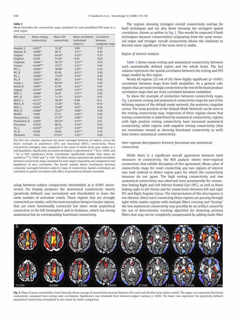
Table 3Mean intensities for connectivity maps calculated for each predefined ROI used as aseed region

ROI name Mean restingconnectivity

Mean DTIconnectivity

Mean correlation(individualsubjects)

Correlationbetweencomposite maps

Angular_L −0.027# 12.10# 0.06 0.39Angular_R 0.008⁎ 46.31 0.11⁎⁎ 0.43CingAnt 0.018⁎⁎ 64.26⁎ 0.23⁎⁎ 0.55CingPost −0.020 91.58⁎ −0.01 0.24Cingulate 0.084⁎⁎ 96.33⁎ 0.23⁎⁎ 0.52Cuneus −0.049## 37.13# 0.12⁎⁎ 0.45IFG_L 0.004⁎⁎ 38.86# 0.10⁎⁎ 0.35IFG_R 0.003⁎ 65.69 0.21⁎⁎ 0.38IPL_L 0.009⁎⁎ 15.55# 0.10⁎⁎ 0.45IPL_R 0.047⁎⁎ 69.21 0.14⁎⁎ 0.42Insula_L 0.051⁎⁎ 84.94⁎ 0.17⁎⁎ 0.49Insula_R 0.047⁎ 63.95 0.25⁎⁎ 0.47Lingual −0.075# 34.08# 0.15⁎⁎ 0.45MFG_L 0.008⁎ 56.47 0.15⁎⁎ 0.42MFG_R 0.011⁎ 71.72⁎ 0.25⁎⁎ 0.47MOcG_L −0.171# 38.36# −0.04 −0.11MOcG_R −0.123# 13.56# −0.01 −0.14MTG_L −0.067# 35.40# 0.07⁎ 0.26MTG_R −0.040# 19.27# 0.08⁎⁎ 0.36MedFG 0.005 67.37 0.20⁎⁎ 0.45Postcentral_L 0.003 27.37# 0.09⁎⁎ 0.32Postcentral_R 0.019⁎ 90.23⁎ 0.15⁎⁎ 0.31Precuneus 0.032⁎ 68.14 0.14⁎⁎ 0.53TG_L −0.035# 22.51# 0.10⁎⁎ 0.39TG_R −0.018 48.86 0.15⁎⁎ 0.35Thalamus 0.023 113.63⁎ 0.22⁎⁎ 0.58

The first two columns represent the mean (averaged between all subject, across thebrain) strength of anatomical (DTI) and functional (RSTC) connectivity. Thoseconnectivity strengths were compared to the mean of whole brain gray matter as anull hypothesis. Significantly increased correlation is represented as ⁎⁎ for pb0.001, and⁎ for pb0.01 significance levels. Correlations significantly smaller than mean aremarked as ## pb0.001 and # pb0.01. The third column represents the spatial correlationbetween connectivity maps calculated for each subject separately and compared to nullhypothesis of zero correlation. The fourth column shows correlations betweencomposite (averaged between subjects) maps of connectivity. Spatial correlations arecalculated as partial correlation with effect of geometrical distance excluded.

558 P. Skudlarski et al. / NeuroImage 43 (2008) 554–561

using between-subject comparisons thresholded at pb0.001 uncor-rected. For display purposes the anatomical connectivity matrix(positively defined) was normalized and thresholded to leave thesame number of activation voxels. Those regions that are stronglyconnected are similar,with themain exception being in insular regions,that are more functionally connected but show weak anatomicalconnection in the left hemisphere and in thalamus, which has stronganatomical but no corresponding functional connectivity.

Fig. 2. Maps of mean connectivity (voxel intensity shows average of connectivity measure beconnectivity calculated from resting state correlations. Significance was estimated from banatomical connectivity normalized to zero mean for better comparison.

The regions showing strongest overall connectivity overlap forboth techniques and are also those showing the strongest spatialcorrelation, shown as yellow in Fig. 1. This would be expected if bothtechniques measure connectivities originating from the same neuro-nal origin and stronger overall connectivity allows the similarity tobecome more significant if the noise level is stable.

Region of interest analysis

Table 3 shows mean resting and anatomical connectivity betweeneach anatomically defined region and the whole brain. The lastcolumn represents the spatial correlation between the resting and DTImaps seeded by this region.

Nearly all regions (22 out of 26) show highly significant (pb0.001)correlation between maps from both modalities. As a general rule,regions that aremost strongly connected to the rest of the brainproducecorrelation maps that are most correlated between modalities.

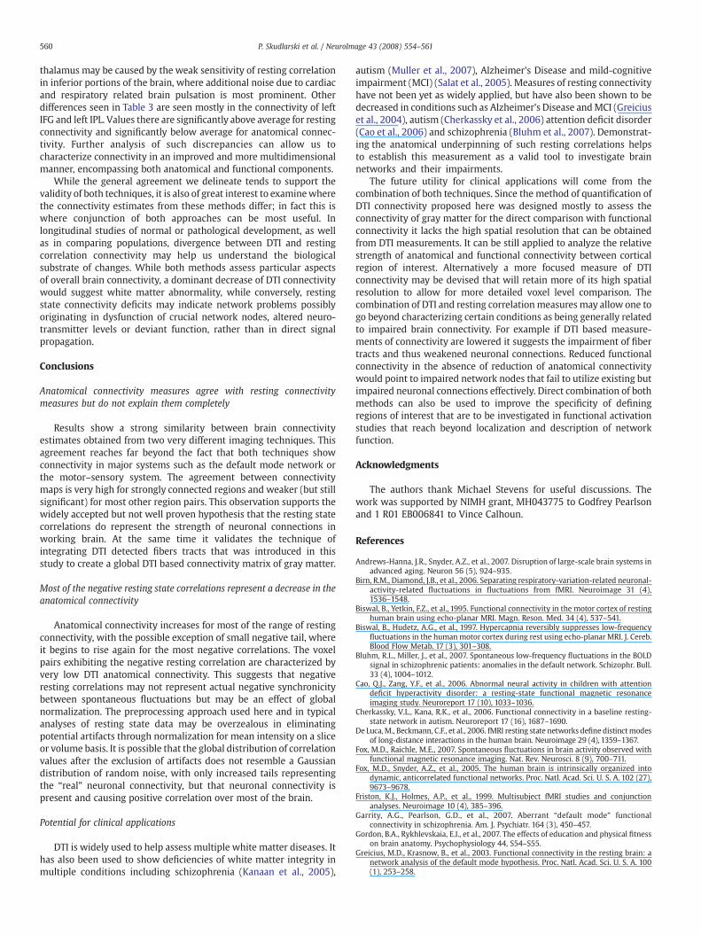
To show the example of similarities between connectivity maps,Fig. 3 presents resting and anatomical connectivitymaps for one of thedefining regions of the default mode network, the posterior cingulatecortex. The main portions of the Default Mode Network can be seen inthe resting connectivity map. Inspection of these regions shows thatresting connectivity is underlined by anatomical connectivity, regionswith high positive resting connectivity have increased anatomicalconnectivity, while regions with negative resting connectivity (thatare sometimes viewed as showing functional connectivity as well)have lowest anatomical connectivity.

Inter-regional discrepancies between functional and anatomicalconnectivity

While there is a significant overall agreement between bothmeasures of connectivity, the ROI analysis shows inter-regionalconnections that exhibit disruption of this agreement. Mean value ofconnectivity maps for voxel connecting any two regions of interestwas rank ordered to detect region pairs for which the connectivitymeasure do not agree. The high resting connectivity and lowanatomical connectivity was observed most prominently for connec-tion linking Right and Left Inferior Frontal Gyri (IFG), as well as thoselinking right to left Insula and for connections between left and rightIFG and Right Angular Gyrus. The interpretation of this discrepancy isnot obvious. Since tracts connecting those regions are passing throughtight white matter regions with multiple fibers crossing and “kissing”the low anatomical connectivity may possibly be an artifact caused bythe use of deterministic tracking algorithm for detecting primaryfibers that may not be completely compensated by adding multi-fiber

tween this voxel and all other gray matter voxels). The upper row represents functionaletween-subject variance pb0.001. The lower row represents the (positively defined)

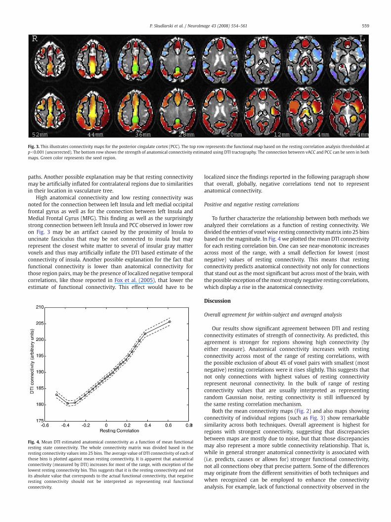
Fig. 3. This illustrates connectivity maps for the posterior cingulate cortex (PCC). The top row represents the functional map based on the resting correlation analysis thresholded atpb0.001 (uncorrected). The bottom row shows the strength of anatomical connectivity estimated using DTI tractography. The connection between vACC and PCC can be seen in bothmaps. Green color represents the seed region.

559P. Skudlarski et al. / NeuroImage 43 (2008) 554–561

paths. Another possible explanation may be that resting connectivitymay be artificially inflated for contralateral regions due to similaritiesin their location in vasculature tree.

High anatomical connectivity and low resting connectivity wasnoted for the connection between left Insula and left medial occipitalfrontal gyrus as well as for the connection between left Insula andMedial Frontal Gyrus (MFG). This finding as well as the surprisinglystrong connection between left Insula and PCC observed in lower rowon Fig. 3 may be an artifact caused by the proximity of Insula touncinate fasciculus that may be not connected to insula but mayrepresent the closest white matter to several of insular gray mattervoxels and thus may artificially inflate the DTI based estimate of theconnectivity of insula. Another possible explanation for the fact thatfunctional connectivity is lower than anatomical connectivity forthose region pairs, may be the presence of localized negative temporalcorrelations, like those reported in Fox et al. (2005), that lower theestimate of functional connectivity. This effect would have to be

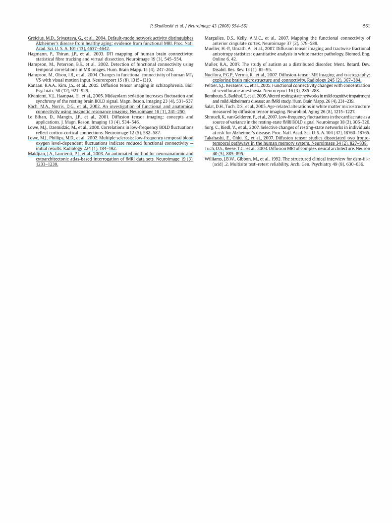
Fig. 4. Mean DTI estimated anatomical connectivity as a function of mean functionalresting state connectivity. The whole connectivity matrix was divided based in theresting connectivity values into 25 bins. The average value of DTI connectivity of each ofthose bins is plotted against mean resting connectivity. It is apparent that anatomicalconnectivity (measured by DTI) increases for most of the range, with exception of thelowest resting connectivity bin. This suggests that it is the resting connectivity and notits absolute value that corresponds to the actual functional connectivity, that negativeresting connectivity should not be interpreted as representing real functionalconnectivity.

localized since the findings reported in the following paragraph showthat overall, globally, negative correlations tend not to representanatomical connectivity.

Positive and negative resting correlations

To further characterize the relationship between both methods weanalyzed their correlations as a function of resting connectivity. Wedivided the entries of voxelwise resting connectivitymatrix into 25 binsbased on the magnitude. In Fig. 4 we plotted themean DTI connectivityfor each resting correlation bin. One can see near-monotonic increasesacross most of the range, with a small deflection for lowest (mostnegative) values of resting connectivity. This means that restingconnectivity predicts anatomical connectivity not only for connectionsthat stand out as the most significant but across most of the brain, withthepossible exceptionof themost strongly negative resting correlations,which display a rise in the anatomical connectivity.

Discussion

Overall agreement for within-subject and averaged analysis

Our results show significant agreement between DTI and restingconnectivity estimates of strength of connectivity. As predicted, thisagreement is stronger for regions showing high connectivity (byeither measure). Anatomical connectivity increases with restingconnectivity across most of the range of resting correlations, withthe possible exclusion of about 4% of voxel pairs with smallest (mostnegative) resting correlations were it rises slightly. This suggests thatnot only connections with highest values of resting connectivityrepresent neuronal connectivity. In the bulk of range of restingconnectivity values that are usually interpreted as representingrandom Gaussian noise, resting connectivity is still influenced bythe same resting correlation mechanism.

Both the mean connectivity maps (Fig. 2) and also maps showingconnectivity of individual regions (such as Fig. 3) show remarkablesimilarity across both techniques. Overall agreement is highest forregions with strongest connectivity, suggesting that discrepanciesbetween maps are mostly due to noise, but that those discrepanciesmay also represent a more subtle connectivity relationship. That is,while in general stronger anatomical connectivity is associated with(i.e. predicts, causes or allows for) stronger functional connectivity,not all connections obey that precise pattern. Some of the differencesmay originate from the different sensitivities of both techniques andwhen recognized can be employed to enhance the connectivityanalysis. For example, lack of functional connectivity observed in the

560 P. Skudlarski et al. / NeuroImage 43 (2008) 554–561

thalamus may be caused by the weak sensitivity of resting correlationin inferior portions of the brain, where additional noise due to cardiacand respiratory related brain pulsation is most prominent. Otherdifferences seen in Table 3 are seen mostly in the connectivity of leftIFG and left IPL. Values there are significantly above average for restingconnectivity and significantly below average for anatomical connec-tivity. Further analysis of such discrepancies can allow us tocharacterize connectivity in an improved and more multidimensionalmanner, encompassing both anatomical and functional components.

While the general agreement we delineate tends to support thevalidity of both techniques, it is also of great interest to examinewherethe connectivity estimates from these methods differ; in fact this iswhere conjunction of both approaches can be most useful. Inlongitudinal studies of normal or pathological development, as wellas in comparing populations, divergence between DTI and restingcorrelation connectivity may help us understand the biologicalsubstrate of changes. While both methods assess particular aspectsof overall brain connectivity, a dominant decrease of DTI connectivitywould suggest white matter abnormality, while conversely, restingstate connectivity deficits may indicate network problems possiblyoriginating in dysfunction of crucial network nodes, altered neuro-transmitter levels or deviant function, rather than in direct signalpropagation.

Conclusions

Anatomical connectivity measures agree with resting connectivitymeasures but do not explain them completely

Results show a strong similarity between brain connectivityestimates obtained from two very different imaging techniques. Thisagreement reaches far beyond the fact that both techniques showconnectivity in major systems such as the default mode network orthe motor–sensory system. The agreement between connectivitymaps is very high for strongly connected regions and weaker (but stillsignificant) for most other region pairs. This observation supports thewidely accepted but not well proven hypothesis that the resting statecorrelations do represent the strength of neuronal connections inworking brain. At the same time it validates the technique ofintegrating DTI detected fibers tracts that was introduced in thisstudy to create a global DTI based connectivity matrix of gray matter.

Most of the negative resting state correlations represent a decrease in theanatomical connectivity

Anatomical connectivity increases for most of the range of restingconnectivity, with the possible exception of small negative tail, whereit begins to rise again for the most negative correlations. The voxelpairs exhibiting the negative resting correlation are characterized byvery low DTI anatomical connectivity. This suggests that negativeresting correlations may not represent actual negative synchronicitybetween spontaneous fluctuations but may be an effect of globalnormalization. The preprocessing approach used here and in typicalanalyses of resting state data may be overzealous in eliminatingpotential artifacts through normalization for mean intensity on a sliceor volume basis. It is possible that the global distribution of correlationvalues after the exclusion of artifacts does not resemble a Gaussiandistribution of random noise, with only increased tails representingthe “real” neuronal connectivity, but that neuronal connectivity ispresent and causing positive correlation over most of the brain.

Potential for clinical applications

DTI is widely used to help assess multiple white matter diseases. Ithas also been used to show deficiencies of white matter integrity inmultiple conditions including schizophrenia (Kanaan et al., 2005),

autism (Muller et al., 2007), Alzheimer's Disease and mild-cognitiveimpairment (MCI) (Salat et al., 2005). Measures of resting connectivityhave not been yet as widely applied, but have also been shown to bedecreased in conditions such as Alzheimer's Disease andMCI (Greiciuset al., 2004), autism (Cherkassky et al., 2006) attention deficit disorder(Cao et al., 2006) and schizophrenia (Bluhm et al., 2007). Demonstrat-ing the anatomical underpinning of such resting correlations helpsto establish this measurement as a valid tool to investigate brainnetworks and their impairments.

The future utility for clinical applications will come from thecombination of both techniques. Since the method of quantification ofDTI connectivity proposed here was designed mostly to assess theconnectivity of gray matter for the direct comparison with functionalconnectivity it lacks the high spatial resolution that can be obtainedfrom DTI measurements. It can be still applied to analyze the relativestrength of anatomical and functional connectivity between corticalregion of interest. Alternatively a more focused measure of DTIconnectivity may be devised that will retain more of its high spatialresolution to allow for more detailed voxel level comparison. Thecombination of DTI and resting correlationmeasures may allow one togo beyond characterizing certain conditions as being generally relatedto impaired brain connectivity. For example if DTI based measure-ments of connectivity are lowered it suggests the impairment of fibertracts and thus weakened neuronal connections. Reduced functionalconnectivity in the absence of reduction of anatomical connectivitywould point to impaired network nodes that fail to utilize existing butimpaired neuronal connections effectively. Direct combination of bothmethods can also be used to improve the specificity of definingregions of interest that are to be investigated in functional activationstudies that reach beyond localization and description of networkfunction.

Acknowledgments

The authors thank Michael Stevens for useful discussions. Thework was supported by NIMH grant, MH043775 to Godfrey Pearlsonand 1 R01 EB006841 to Vince Calhoun.

References

Andrews-Hanna, J.R., Snyder, A.Z., et al., 2007. Disruption of large-scale brain systems inadvanced aging. Neuron 56 (5), 924–935.

Birn, R.M., Diamond, J.B., et al., 2006. Separating respiratory-variation-related neuronal-activity-related fluctuations in fluctuations from fMRI. Neuroimage 31 (4),1536–1548.

Biswal, B., Yetkin, F.Z., et al., 1995. Functional connectivity in the motor cortex of restinghuman brain using echo-planar MRI. Magn. Reson. Med. 34 (4), 537–541.

Biswal, B., Hudetz, A.G., et al., 1997. Hypercapnia reversibly suppresses low-frequencyfluctuations in the humanmotor cortex during rest using echo-planar MRI. J. Cereb.Blood Flow Metab. 17 (3), 301–308.

Bluhm, R.L., Miller, J., et al., 2007. Spontaneous low-frequency fluctuations in the BOLDsignal in schizophrenic patients: anomalies in the default network. Schizophr. Bull.33 (4), 1004–1012.

Cao, Q.J., Zang, Y.F., et al., 2006. Abnormal neural activity in children with attentiondeficit hyperactivity disorder: a resting-state functional magnetic resonanceimaging study. Neuroreport 17 (10), 1033–1036.

Cherkassky, V.L., Kana, R.K., et al., 2006. Functional connectivity in a baseline resting-state network in autism. Neuroreport 17 (16), 1687–1690.

De Luca, M., Beckmann, C.F., et al., 2006. fMRI resting state networks define distinctmodesof long-distance interactions in the human brain. Neuroimage 29 (4), 1359–1367.

Fox, M.D., Raichle, M.E., 2007. Spontaneous fluctuations in brain activity observed withfunctional magnetic resonance imaging. Nat. Rev. Neurosci. 8 (9), 700–711.

Fox, M.D., Snyder, A.Z., et al., 2005. The human brain is intrinsically organized intodynamic, anticorrelated functional networks. Proc. Natl. Acad. Sci. U. S. A. 102 (27),9673–9678.

Friston, K.J., Holmes, A.P., et al., 1999. Multisubject fMRI studies and conjunctionanalyses. Neuroimage 10 (4), 385–396.

Garrity, A.G., Pearlson, G.D., et al., 2007. Aberrant “default mode” functionalconnectivity in schizophrenia. Am. J. Psychiatr. 164 (3), 450–457.

Gordon, B.A., Rykhlevskaia, E.I., et al., 2007. The effects of education and physical fitnesson brain anatomy. Psychophysiology 44, S54–S55.

Greicius, M.D., Krasnow, B., et al., 2003. Functional connectivity in the resting brain: anetwork analysis of the default mode hypothesis. Proc. Natl. Acad. Sci. U. S. A. 100(1), 253–258.

561P. Skudlarski et al. / NeuroImage 43 (2008) 554–561

Greicius, M.D., Srivastava, G., et al., 2004. Default-mode network activity distinguishesAlzheimer's disease from healthy aging: evidence from functional MRI. Proc. Natl.Acad. Sci. U. S. A. 101 (13), 4637–4642.

Hagmann, P., Thiran, J.P., et al., 2003. DTI mapping of human brain connectivity:statistical fibre tracking and virtual dissection. Neuroimage 19 (3), 545–554.

Hampson, M., Peterson, B.S., et al., 2002. Detection of functional connectivity usingtemporal correlations in MR images. Hum. Brain Mapp. 15 (4), 247–262.

Hampson, M., Olson, I.R., et al., 2004. Changes in functional connectivity of human MT/V5 with visual motion input. Neuroreport 15 (8), 1315–1319.

Kanaan, R.A.A., Kim, J.S., et al., 2005. Diffusion tensor imaging in schizophrenia. Biol.Psychiatr. 58 (12), 921–929.

Kiviniemi, V.J., Haanpaa, H., et al., 2005. Midazolarn sedation increases fluctuation andsynchrony of the resting brain BOLD signal. Magn. Reson. Imaging 23 (4), 531–537.

Koch, M.A., Norris, D.G., et al., 2002. An investigation of functional and anatomicalconnectivity using magnetic resonance imaging. Neuroimage 16 (1), 241–250.

Le Bihan, D., Mangin, J.F., et al., 2001. Diffusion tensor imaging: concepts andapplications. J. Magn. Reson. Imaging 13 (4), 534–546.

Lowe, M.J., Dzemidzic, M., et al., 2000. Correlations in low-frequency BOLD fluctuationsreflect cortico-cortical connections. Neuroimage 12 (5), 582–587.

Lowe, M.J., Phillips, M.D., et al., 2002. Multiple sclerosis: low-frequency temporal bloodoxygen level-dependent fluctuations indicate reduced functional connectivity —initial results. Radiology 224 (1), 184–192.

Maldjian, J.A., Laurienti, P.J., et al., 2003. An automated method for neuroanatomic andcytoarchitectonic atlas-based interrogation of fMRI data sets. Neuroimage 19 (3),1233–1239.

Margulies, D.S., Kelly, A.M.C., et al., 2007. Mapping the functional connectivity ofanterior cingulate cortex. Neuroimage 37 (2), 579–588.

Mueller, H.-P., Unrath, A., et al., 2007. Diffusion tensor imaging and tractwise fractionalanisotropy statistics: quantitative analysis in white matter pathology. Biomed. Eng.Online 6, 42.

Muller, R.A., 2007. The study of autism as a distributed disorder. Ment. Retard. Dev.Disabil. Res. Rev. 13 (1), 85–95.

Nucifora, P.G.P., Verma, R., et al., 2007. Diffusion-tensor MR Imaging and tractography:exploring brain microstructure and connectivity. Radiology 245 (2), 367–384.

Peltier, S.J., Kerssens, C., et al., 2005. Functional connectivity changes with concentrationof sevoflurane anesthesia. Neuroreport 16 (3), 285–288.

Rombouts, S., Barkhof, F., et al., 2005.Alteredrestingstatenetworks inmildcognitive impairmentand mild Alzheimer's disease: an fMRI study. Hum. Brain Mapp. 26 (4), 231–239.

Salat, D.H., Tuch, D.S., et al., 2005. Age-related alterations inwhitemattermicrostructuremeasured by diffusion tensor imaging. Neurobiol. Aging 26 (8), 1215–1227.

Shmueli, K., vanGelderen, P., et al., 2007. Low-frequencyfluctuations in the cardiac rate as asource of variance in the resting-state fMRI BOLD signal. Neuroimage 38 (2), 306–320.

Sorg, C., Riedl, V., et al., 2007. Selective changes of resting-state networks in individualsat risk for Alzheimer's disease. Proc. Natl. Acad. Sci. U. S. A. 104 (47), 18760–18765.

Takahashi, E., Ohki, K., et al., 2007. Diffusion tensor studies dissociated two fronto-temporal pathways in the human memory system. Neuroimage 34 (2), 827–838.

Tuch, D.S., Reese, T.G., et al., 2003. DiffusionMRI of complex neural architecture. Neuron40 (5), 885–895.

Williams, J.B.W., Gibbon, M., et al., 1992. The structured clinical interview for dsm-iii-r(scid) .2. Multisite test–retest reliability. Arch. Gen. Psychiatry 49 (8), 630–636.