ANALYZING, IMPROVING, AND LEVERAGING CROWDSOURCED VISUAL KNOWLEDGE REPRESENTATIONS A THESIS SUBMITTED TO THE DEPARTMENT OF COMPUTER SCIENCE AND THE COMMITTEE ON GRADUATE STUDIES OF STANFORD UNIVERSITY IN PARTIAL FULFILLMENT OF THE REQUIREMENTS FOR THE DEGREE OF MASTERS OF SCIENCE Kenji Hata June 2017

Welcome message from author
This document is posted to help you gain knowledge. Please leave a comment to let me know what you think about it! Share it to your friends and learn new things together.
Transcript
ANALYZING, IMPROVING, AND LEVERAGING CROWDSOURCED VISUAL
KNOWLEDGE REPRESENTATIONS
A THESIS
SUBMITTED TO THE DEPARTMENT OF COMPUTER SCIENCE
AND THE COMMITTEE ON GRADUATE STUDIES
OF STANFORD UNIVERSITY
IN PARTIAL FULFILLMENT OF THE REQUIREMENTS
FOR THE DEGREE OF
MASTERS OF SCIENCE
Kenji Hata
June 2017

c© Copyright by Kenji Hata 2017
All Rights Reserved
ii

I certify that I have read this dissertation and that, in my opinion, it is fully adequate
in scope and quality as a dissertation for the degree of Masters of Science.
(Fei-Fei Li) Principal Co-Advisor
I certify that I have read this dissertation and that, in my opinion, it is fully adequate
in scope and quality as a dissertation for the degree of Masters of Science.
(Michael Bernstein) Principal Co-Advisor
Approved for the University Committee on Graduate Studies
iii
Acknowledgements
First and foremost, I would like to express my utmost appreciation to my advisors Fei-Fei Li and
Michael Bernstein for both nurturing my growth as a researcher and believing in me throughout my
time at Stanford. Their guidance greatly developed my own maturity as a researcher and as a person.
I would also like to thank Oussama Khatib and Allison Okamura for sparking my initial interest
in research as an undergraduate at Stanford. I thank Silvio Savarese for his support and guidance
throughout my research career. I thank Ranjay Krishna for mentoring me throughout my Master’s
program at Stanford.
Next, I would like to thank my co-authors, whom I have had the greatest joy working with and
learning from. In alphabetical order, they are: Andrew Stanley, Allison Okamura, David Ayman
Shamma, Frederic Ren, Joshua Kravitz, Juan Carlos Niebles, Justin Johnson, Li Fei-Fei, Michael
Bernstein, Oliver Groth, Ranjay Krishna, Sherman Leung, Stephanie Chen, Yannis Kalanditis, and
Yuke Zhu. More broadly, I give my appreciation to members of the Stanford Vision and Learning
Lab and the Stanford HCI Lab, whose helpful discussions helped propel these works forward.
Finally, I would like to thank my parents, family, and friends for always believing in my throughout
every step in life. It has been a great ride so far, and I cannot wait for what is next.
iv
Contents
Acknowledgements iv
1 Introduction 1
1.1 Motivation . . . . . . . . . . . . . . . . . . . . . . . . . . . . . . . . . . . . . . . . . 1
1.2 Thesis Outline . . . . . . . . . . . . . . . . . . . . . . . . . . . . . . . . . . . . . . . 1
1.3 Previously Published Papers . . . . . . . . . . . . . . . . . . . . . . . . . . . . . . . . 2
2 Visual Genome 3
2.1 Introduction . . . . . . . . . . . . . . . . . . . . . . . . . . . . . . . . . . . . . . . . . 3
2.2 Related Work . . . . . . . . . . . . . . . . . . . . . . . . . . . . . . . . . . . . . . . . 9
2.2.1 Datasets . . . . . . . . . . . . . . . . . . . . . . . . . . . . . . . . . . . . . . . 9
2.2.2 Image Descriptions . . . . . . . . . . . . . . . . . . . . . . . . . . . . . . . . . 11
2.2.3 Objects . . . . . . . . . . . . . . . . . . . . . . . . . . . . . . . . . . . . . . . 11
2.2.4 Attributes . . . . . . . . . . . . . . . . . . . . . . . . . . . . . . . . . . . . . . 12
2.2.5 Relationships . . . . . . . . . . . . . . . . . . . . . . . . . . . . . . . . . . . . 12
2.2.6 Question Answering . . . . . . . . . . . . . . . . . . . . . . . . . . . . . . . . 13
2.2.7 Knowledge Representation . . . . . . . . . . . . . . . . . . . . . . . . . . . . . 13
2.3 Visual Genome Data Representation . . . . . . . . . . . . . . . . . . . . . . . . . . . 14
2.3.1 Multiple regions and their descriptions . . . . . . . . . . . . . . . . . . . . . . 14
2.3.2 Multiple objects and their bounding boxes . . . . . . . . . . . . . . . . . . . . 15
2.3.3 A set of attributes . . . . . . . . . . . . . . . . . . . . . . . . . . . . . . . . . 15
2.3.4 A set of relationships . . . . . . . . . . . . . . . . . . . . . . . . . . . . . . . . 16
2.3.5 A set of region graphs . . . . . . . . . . . . . . . . . . . . . . . . . . . . . . . 16
2.3.6 One scene graph . . . . . . . . . . . . . . . . . . . . . . . . . . . . . . . . . . 17
2.3.7 A set of question answer pairs . . . . . . . . . . . . . . . . . . . . . . . . . . . 17
2.4 Dataset Statistics and Analysis . . . . . . . . . . . . . . . . . . . . . . . . . . . . . . 18
2.4.1 Image Selection . . . . . . . . . . . . . . . . . . . . . . . . . . . . . . . . . . . 19
2.4.2 Region Description Statistics . . . . . . . . . . . . . . . . . . . . . . . . . . . 20
v
2.4.3 Object Statistics . . . . . . . . . . . . . . . . . . . . . . . . . . . . . . . . . . 25
2.4.4 Attribute Statistics . . . . . . . . . . . . . . . . . . . . . . . . . . . . . . . . . 26
2.4.5 Relationship Statistics . . . . . . . . . . . . . . . . . . . . . . . . . . . . . . . 30
2.4.6 Region and Scene Graph Statistics . . . . . . . . . . . . . . . . . . . . . . . . 32
2.4.7 Question Answering Statistics . . . . . . . . . . . . . . . . . . . . . . . . . . . 35
2.4.8 Canonicalization Statistics . . . . . . . . . . . . . . . . . . . . . . . . . . . . . 37
3 Crowdsourcing Strategies 42
3.0.1 Crowd Workers . . . . . . . . . . . . . . . . . . . . . . . . . . . . . . . . . . . 42
3.0.2 Region Descriptions . . . . . . . . . . . . . . . . . . . . . . . . . . . . . . . . 43
3.0.3 Objects . . . . . . . . . . . . . . . . . . . . . . . . . . . . . . . . . . . . . . . 44
3.0.4 Attributes, Relationships, and Region Graphs . . . . . . . . . . . . . . . . . . 45
3.0.5 Scene Graphs . . . . . . . . . . . . . . . . . . . . . . . . . . . . . . . . . . . . 46
3.0.6 Questions and Answers . . . . . . . . . . . . . . . . . . . . . . . . . . . . . . 46
3.0.7 Verification . . . . . . . . . . . . . . . . . . . . . . . . . . . . . . . . . . . . . 47
3.0.8 Canonicalization . . . . . . . . . . . . . . . . . . . . . . . . . . . . . . . . . . 48
4 Embracing Error to Enable Rapid Crowdsourcing 50
4.1 Introduction . . . . . . . . . . . . . . . . . . . . . . . . . . . . . . . . . . . . . . . . . 50
4.2 Related Work . . . . . . . . . . . . . . . . . . . . . . . . . . . . . . . . . . . . . . . . 52
4.3 Error-Embracing Crowdsourcing . . . . . . . . . . . . . . . . . . . . . . . . . . . . . 54
4.3.1 Rapid crowdsourcing of binary decision tasks . . . . . . . . . . . . . . . . . . 55
4.3.2 Multi-Class Classification for Categorical Data . . . . . . . . . . . . . . . . . 57
4.4 Model . . . . . . . . . . . . . . . . . . . . . . . . . . . . . . . . . . . . . . . . . . . . 57
4.5 Calibration: Baseline Worker Reaction Time . . . . . . . . . . . . . . . . . . . . . . 58
4.6 Study 1: Image Verification . . . . . . . . . . . . . . . . . . . . . . . . . . . . . . . . 60
4.7 Study 2: Non-Visual Tasks . . . . . . . . . . . . . . . . . . . . . . . . . . . . . . . . 63
4.8 Study 3: Multi-class Classification . . . . . . . . . . . . . . . . . . . . . . . . . . . . 64
4.9 Application: Building ImageNet . . . . . . . . . . . . . . . . . . . . . . . . . . . . . . 65
4.10 Discussion . . . . . . . . . . . . . . . . . . . . . . . . . . . . . . . . . . . . . . . . . . 66
4.11 Conclusion . . . . . . . . . . . . . . . . . . . . . . . . . . . . . . . . . . . . . . . . . 67
4.12 Supplementary Material . . . . . . . . . . . . . . . . . . . . . . . . . . . . . . . . . . 67
4.12.1 Runtime Analysis for Class-Optimized Classification . . . . . . . . . . . . . . 67
5 Long-Term Crowd Worker Quality 69
5.1 Introduction . . . . . . . . . . . . . . . . . . . . . . . . . . . . . . . . . . . . . . . . . 69
5.2 Related Work . . . . . . . . . . . . . . . . . . . . . . . . . . . . . . . . . . . . . . . . 71
5.2.1 Fatigue . . . . . . . . . . . . . . . . . . . . . . . . . . . . . . . . . . . . . . . 71
vi
5.2.2 Satisficing . . . . . . . . . . . . . . . . . . . . . . . . . . . . . . . . . . . . . . 71
5.2.3 The global crowdsourcing ecosystem . . . . . . . . . . . . . . . . . . . . . . . 72
5.2.4 Improving crowdsourcing quality . . . . . . . . . . . . . . . . . . . . . . . . . 72
5.3 Analysis: Long-Term Crowdsourcing Trends . . . . . . . . . . . . . . . . . . . . . . . 73
5.3.1 Data . . . . . . . . . . . . . . . . . . . . . . . . . . . . . . . . . . . . . . . . . 73
5.3.2 Workers are consistent over long periods . . . . . . . . . . . . . . . . . . . . . 75
5.3.3 Discussion . . . . . . . . . . . . . . . . . . . . . . . . . . . . . . . . . . . . . . 79
5.4 Experiment: Why Are Workers Consistent? . . . . . . . . . . . . . . . . . . . . . . . 79
5.4.1 Task . . . . . . . . . . . . . . . . . . . . . . . . . . . . . . . . . . . . . . . . . 80
5.4.2 Experiment Setup . . . . . . . . . . . . . . . . . . . . . . . . . . . . . . . . . 82
5.4.3 Data Collected . . . . . . . . . . . . . . . . . . . . . . . . . . . . . . . . . . . 83
5.4.4 Results . . . . . . . . . . . . . . . . . . . . . . . . . . . . . . . . . . . . . . . 83
5.4.5 Discussion . . . . . . . . . . . . . . . . . . . . . . . . . . . . . . . . . . . . . . 84
5.5 Predicting From Small Glimpses . . . . . . . . . . . . . . . . . . . . . . . . . . . . . 85
5.5.1 Experimental Setup . . . . . . . . . . . . . . . . . . . . . . . . . . . . . . . . 86
5.5.2 Results . . . . . . . . . . . . . . . . . . . . . . . . . . . . . . . . . . . . . . . 87
5.5.3 Discussion . . . . . . . . . . . . . . . . . . . . . . . . . . . . . . . . . . . . . . 87
5.6 Implications for Crowdsourcing . . . . . . . . . . . . . . . . . . . . . . . . . . . . . . 87
5.7 Conclusion . . . . . . . . . . . . . . . . . . . . . . . . . . . . . . . . . . . . . . . . . 88
6 Leveraging Representations in Visual Genome 90
6.1 Introduction . . . . . . . . . . . . . . . . . . . . . . . . . . . . . . . . . . . . . . . . . 90
6.1.1 Attribute Prediction . . . . . . . . . . . . . . . . . . . . . . . . . . . . . . . . 91
6.1.2 Relationship Prediction . . . . . . . . . . . . . . . . . . . . . . . . . . . . . . 93
6.1.3 Generating Region Descriptions . . . . . . . . . . . . . . . . . . . . . . . . . . 95
6.1.4 Question Answering . . . . . . . . . . . . . . . . . . . . . . . . . . . . . . . . 96
7 Dense-Captioning Events in Videos 99
7.1 Introduction . . . . . . . . . . . . . . . . . . . . . . . . . . . . . . . . . . . . . . . . . 99
7.2 Related work . . . . . . . . . . . . . . . . . . . . . . . . . . . . . . . . . . . . . . . . 101
7.3 Dense-captioning events model . . . . . . . . . . . . . . . . . . . . . . . . . . . . . . 103
7.3.1 Event proposal module . . . . . . . . . . . . . . . . . . . . . . . . . . . . . . . 104
7.3.2 Captioning module with context . . . . . . . . . . . . . . . . . . . . . . . . . 104
7.3.3 Implementation details. . . . . . . . . . . . . . . . . . . . . . . . . . . . . . . 105
7.4 ActivityNet Captions dataset . . . . . . . . . . . . . . . . . . . . . . . . . . . . . . . 106
7.4.1 Dataset statistics . . . . . . . . . . . . . . . . . . . . . . . . . . . . . . . . . . 107
7.4.2 Temporal agreement amongst annotators . . . . . . . . . . . . . . . . . . . . 108
7.5 Experiments . . . . . . . . . . . . . . . . . . . . . . . . . . . . . . . . . . . . . . . . . 108
vii
7.5.1 Dense-captioning events . . . . . . . . . . . . . . . . . . . . . . . . . . . . . . 108
7.5.2 Event localization . . . . . . . . . . . . . . . . . . . . . . . . . . . . . . . . . 112
7.5.3 Video and paragraph retrieval . . . . . . . . . . . . . . . . . . . . . . . . . . . 112
7.6 Conclusion . . . . . . . . . . . . . . . . . . . . . . . . . . . . . . . . . . . . . . . . . 113
7.7 Supplementary material . . . . . . . . . . . . . . . . . . . . . . . . . . . . . . . . . . 113
7.7.1 Comparison to other datasets. . . . . . . . . . . . . . . . . . . . . . . . . . . 113
7.7.2 Detailed dataset statistics . . . . . . . . . . . . . . . . . . . . . . . . . . . . . 114
7.7.3 Dataset collection process . . . . . . . . . . . . . . . . . . . . . . . . . . . . . 115
7.7.4 Annotation details . . . . . . . . . . . . . . . . . . . . . . . . . . . . . . . . . 117
8 Conclusion 121
Bibliography 122
viii

List of Tables
2.1 A comparison of existing datasets with Visual Genome. We show that Visual Genome
has an order of magnitude more descriptions and question answers. It also has a more
diverse set of object, attribute, and relationship classes. Additionally, Visual Genome
contains a higher density of these annotations per image. The number of distinct
categories in Visual Genome are calculated by lower-casing and stemming names of
objects, attributes and relationships. . . . . . . . . . . . . . . . . . . . . . . . . . . . 10
2.2 Comparison of Visual Genome objects and categories to related datasets. . . . . . . 24
2.3 The average number of objects, attributes, and relationships per region graph and per
scene graph. . . . . . . . . . . . . . . . . . . . . . . . . . . . . . . . . . . . . . . . . . 32
2.4 Precision, recall, and mapping accuracy percentages for object, attribute, and rela-
tionship canonicalization. . . . . . . . . . . . . . . . . . . . . . . . . . . . . . . . . . 38
3.1 Geographic distribution of countries from where crowd workers contributed to Visual
Genome. . . . . . . . . . . . . . . . . . . . . . . . . . . . . . . . . . . . . . . . . . . . 43
4.1 We compare the conventional approach for binary verification tasks (image verification,
sentiment analysis, word similarity and topic detection) with our technique and
compute precision and recall scores. Precision scores, recall scores and speedups are
calculated using 3 workers in the conventional setting. Image verification, sentiment
analysis and word similarity used 5 workers using our technique, while topic detection
used only 2 workers. We also show the time taken (in seconds) for 1 worker to do each
task. . . . . . . . . . . . . . . . . . . . . . . . . . . . . . . . . . . . . . . . . . . . . . 60
5.1 The number of workers, tasks, and annotations collected for image descriptions,
question answering, and verifications. . . . . . . . . . . . . . . . . . . . . . . . . . . . 74
5.2 Data collected from the verification experiment. A total of 1, 134 workers were divided
up into four conditions, with a high or low threshold and transparency. . . . . . . . . 84
ix
6.1 (First row) Results for the attribute prediction task where we only predict attributes
for a given image crop. (Second row) Attribute-object prediction experiment where
we predict both the attributes as well as the object from a given crop of the image. . 93
6.2 Results for relationship classification (first row) and joint classification (second row)
experiments. . . . . . . . . . . . . . . . . . . . . . . . . . . . . . . . . . . . . . . . . 95
6.3 Results for the region description generation experiment. Scores in the first row are for
the region descriptions generated from the NeuralTalk model trained on Flickr8K, and
those in the second row are for those generated by the model trained on Visual Genome
data. BLEU, CIDEr, and METEOR scores all compare the predicted description to a
ground truth in different ways. . . . . . . . . . . . . . . . . . . . . . . . . . . . . . . 97
6.4 Baseline QA performances in the 6 different question types. We report human
evaluation as well as a baseline method that predicts the most frequently occurring
answer in the dataset. . . . . . . . . . . . . . . . . . . . . . . . . . . . . . . . . . . . 97
7.1 We report Bleu (B), METEOR (M) and CIDEr (C) captioning scores for the task
of dense-captioning events. On the top table, we report performances of just our
captioning module with ground truth proposals. On the bottom table, we report the
combined performances of our complete model, with proposals predicted from our
proposal module. Since prior work has focused only on describing entire videos and
not also detecting a series of events, we only compare existing video captioning models
using ground truth proposals. . . . . . . . . . . . . . . . . . . . . . . . . . . . . . . . 107
7.2 We report the effects of context on captioning the 1st, 2nd and 3rd events in a video.
We see that performance increases with the addition of past context in the online
model and with future context in full model. . . . . . . . . . . . . . . . . . . . . . . 109
7.3 Results for video and paragraph retrieval. We see that the utilization of context to
encode video events help us improve retrieval. R@k measures the recall at varying
thresholds k and med. rank measures the median rank the retrieval. . . . . . . . . . 111
7.4 Compared to other video datasets, ActivityNet Captions (ANC) contains long videos
with a large number of sentences that are all temporally localized and is the only dataset
that contains overlapping events. (Loc. shows which datasets contain temporally
localized language descriptions. Bold fonts are used to highlight the nearest comparison
of our model with existing models.) . . . . . . . . . . . . . . . . . . . . . . . . . . . . 115
x
List of Figures
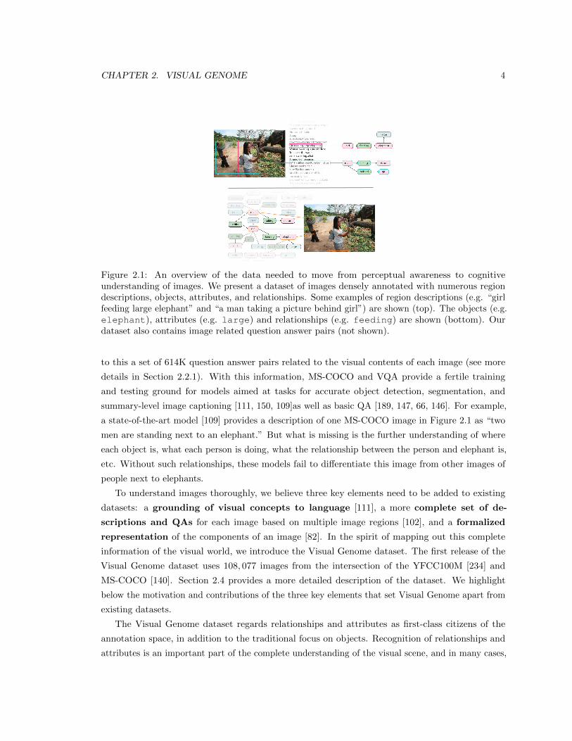
2.1 An overview of the data needed to move from perceptual awareness to cognitive
understanding of images. We present a dataset of images densely annotated with
numerous region descriptions, objects, attributes, and relationships. Some examples
of region descriptions (e.g. “girl feeding large elephant” and “a man taking a picture
behind girl”) are shown (top). The objects (e.g. elephant), attributes (e.g. large)
and relationships (e.g. feeding) are shown (bottom). Our dataset also contains
image related question answer pairs (not shown). . . . . . . . . . . . . . . . . . . . . 4
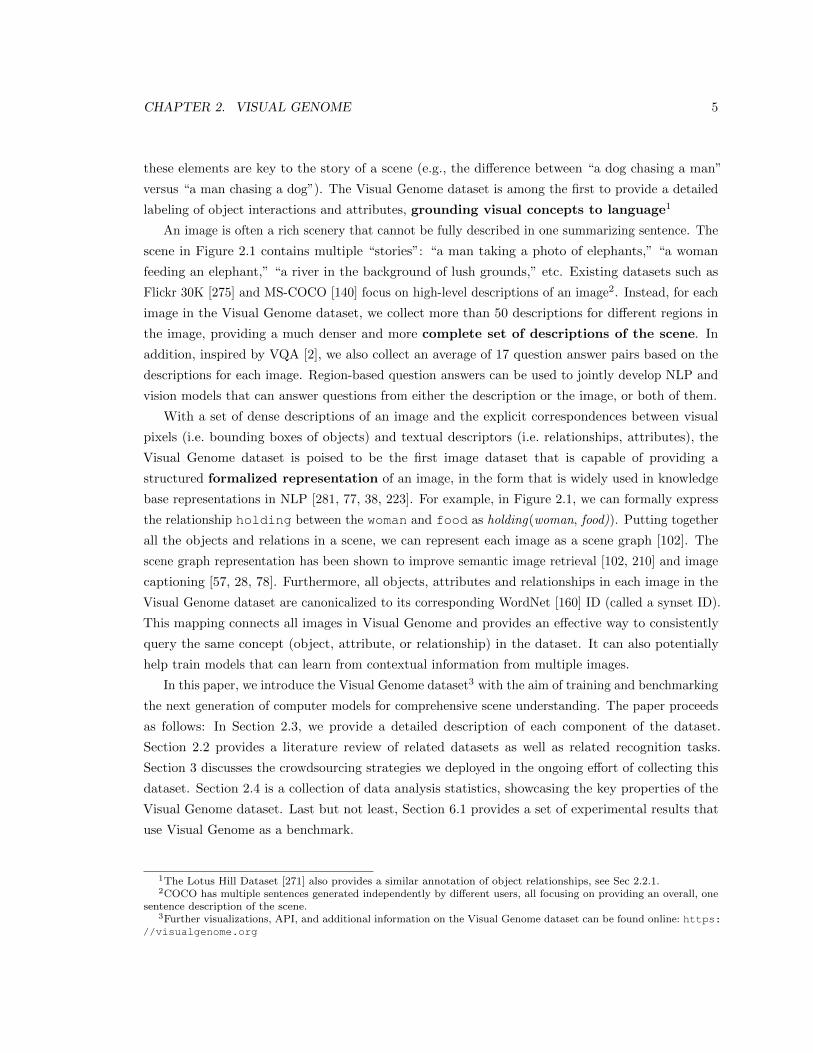
2.2 An example image from the Visual Genome dataset. We show 3 region descriptions
and their corresponding region graphs. We also show the connected scene graph
collected by combining all of the image’s region graphs. The top region description
is “a man and a woman sit on a park bench along a river.” It contains the objects:
man, woman, bench and river. The relationships that connect these objects are:
sits on(man, bench), in front of (man, river), and sits on(woman, bench). . . . . . . 6
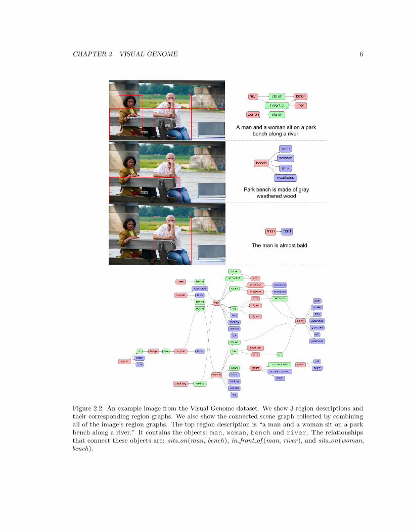
2.3 An example image from our dataset along with its scene graph representation. The
scene graph contains objects (child, instructor, helmet, etc.) that are localized
in the image as bounding boxes (not shown). These objects also have attributes:
large, green, behind, etc. Finally, objects are connected to each other through
relationships: wears(child, helmet), wears(instructor, jacket), etc. . . . . . . . . . . . 7
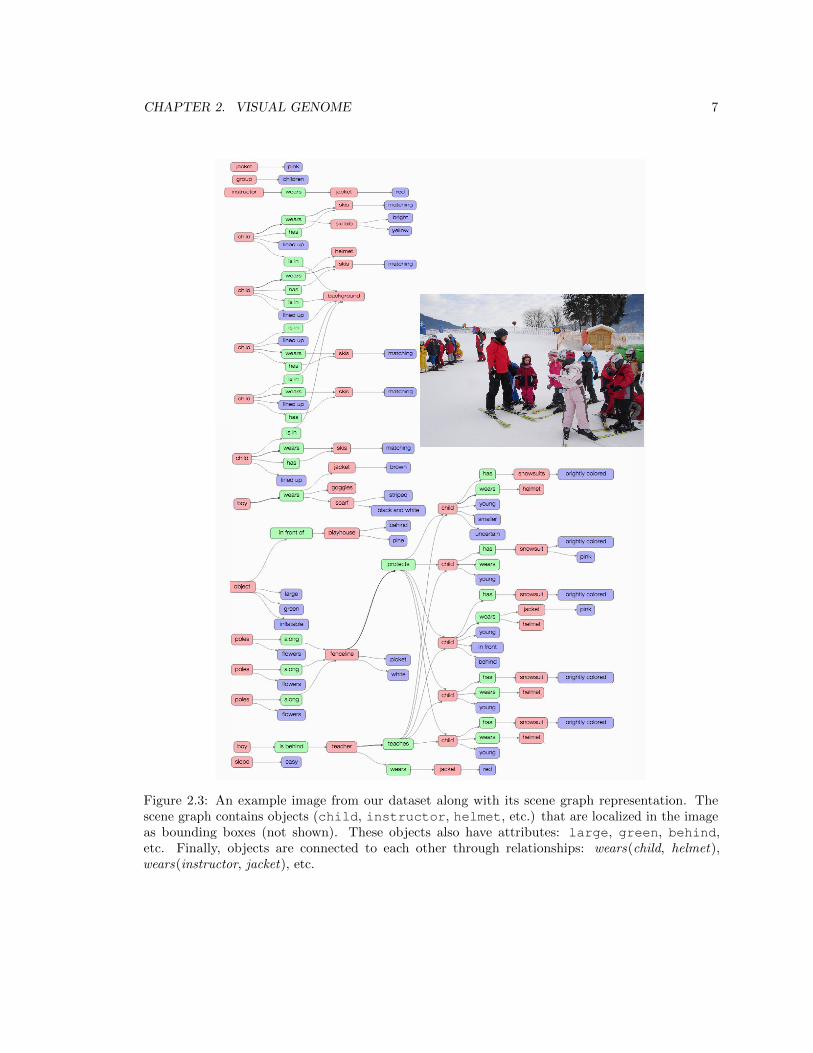
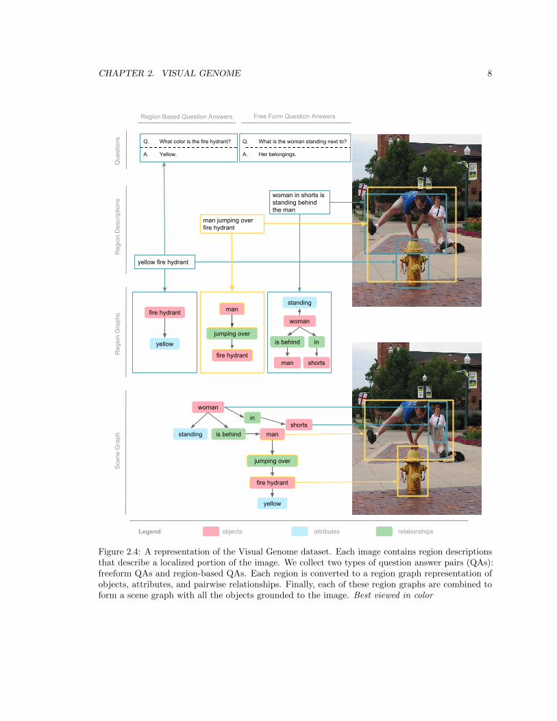
2.4 A representation of the Visual Genome dataset. Each image contains region descriptions
that describe a localized portion of the image. We collect two types of question answer
pairs (QAs): freeform QAs and region-based QAs. Each region is converted to a region
graph representation of objects, attributes, and pairwise relationships. Finally, each of
these region graphs are combined to form a scene graph with all the objects grounded
to the image. Best viewed in color . . . . . . . . . . . . . . . . . . . . . . . . . . . . 8
xi
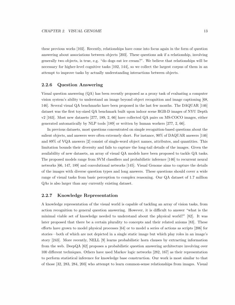
2.5 To describe all the contents of and interactions in an image, the Visual Genome
dataset includes multiple human-generated image regions descriptions, with each
region localized by a bounding box. Here, we show three regions descriptions on
various image regions: “man jumping over a fire hydrant,” “yellow fire hydrant,” and
“woman in shorts is standing behind the man.” . . . . . . . . . . . . . . . . . . . . . 14
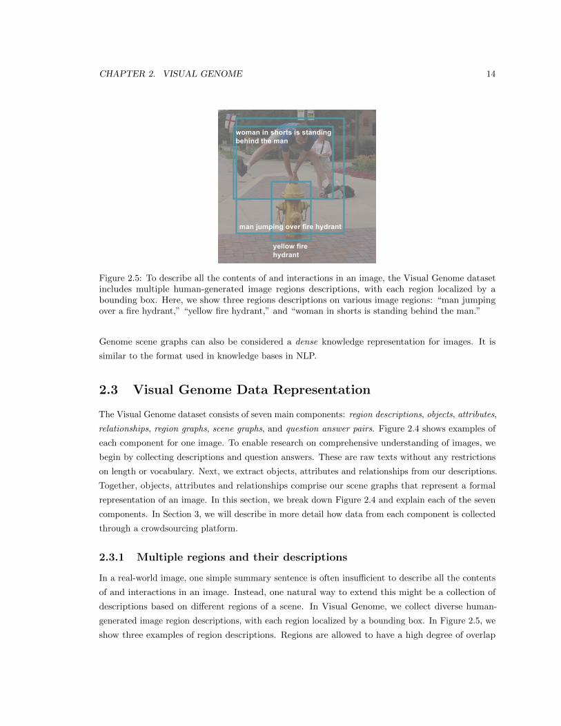
2.6 From all of the region descriptions, we extract all objects mentioned. For example,
from the region description “man jumping over a fire hydrant,” we extract man and
fire hydrant. . . . . . . . . . . . . . . . . . . . . . . . . . . . . . . . . . . . . . . 15
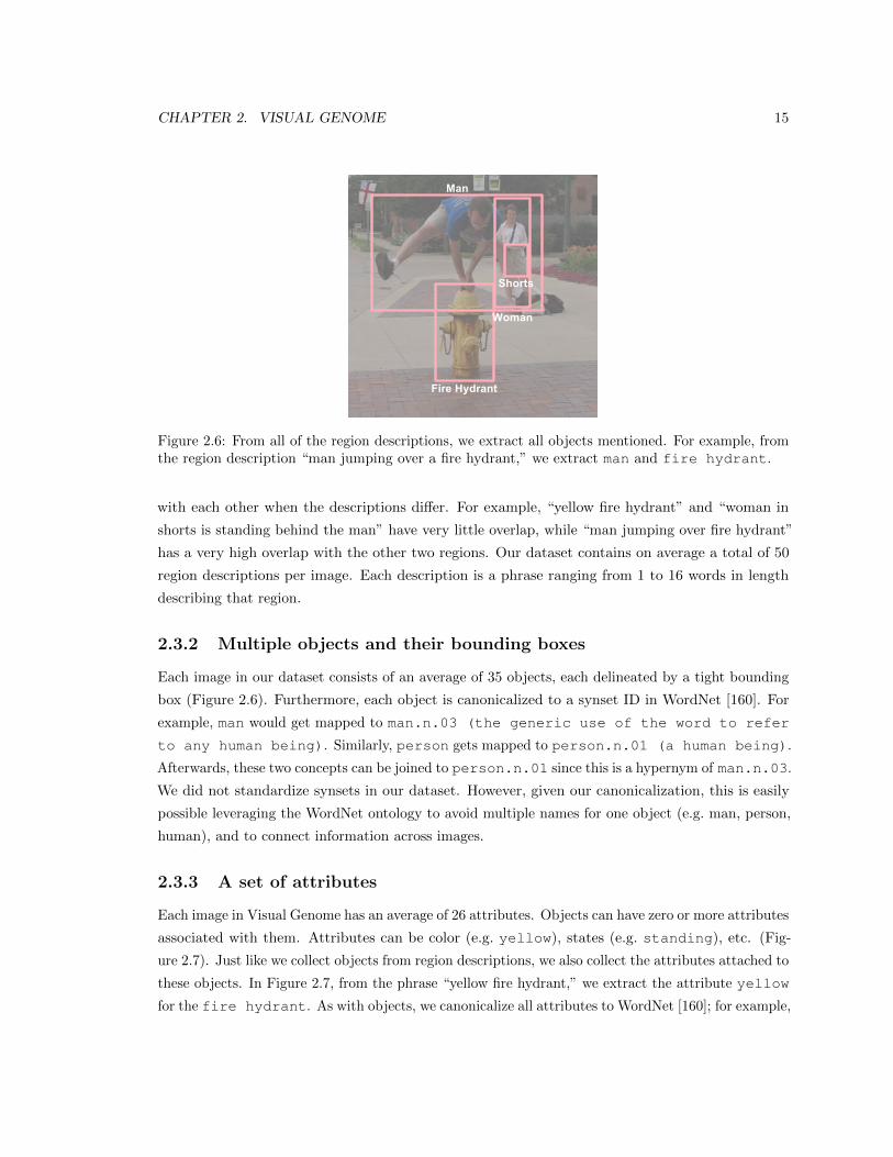
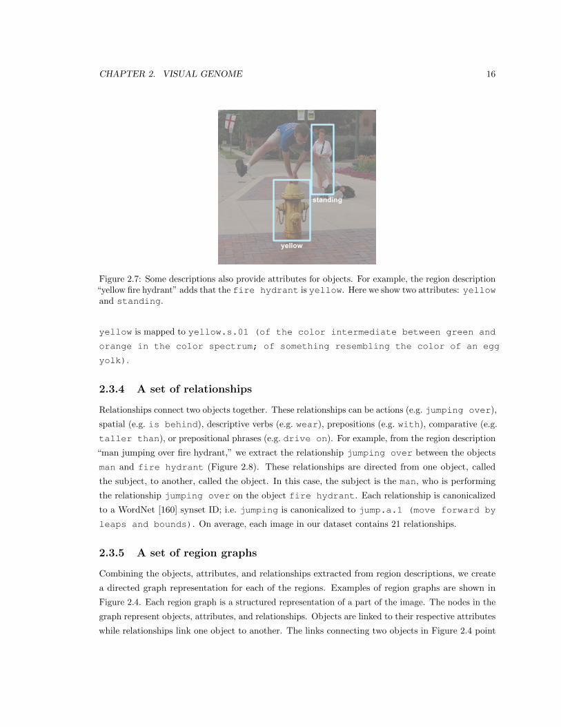
2.7 Some descriptions also provide attributes for objects. For example, the region descrip-
tion “yellow fire hydrant” adds that the fire hydrant is yellow. Here we show
two attributes: yellow and standing. . . . . . . . . . . . . . . . . . . . . . . . . . 16
2.8 Our dataset also captures the relationships and interactions between objects in our
images. In this example, we show the relationship jumping over between the objects
man and fire hydrant. . . . . . . . . . . . . . . . . . . . . . . . . . . . . . . . . . 17
2.9 A distribution of the top 25 image synsets in the Visual Genome dataset. A variety of
synsets are well represented in the dataset, with the top 25 synsets having at least
800 example images each. Note that an image synset is the label of the entire image
according to the ImageNet ontology and are separate from the synsets for objects,
attributes and relationships. . . . . . . . . . . . . . . . . . . . . . . . . . . . . . . . . 18
2.10 (a) An example image from the dataset with its region descriptions. We only display
localizations for 6 of the 50 descriptions to avoid clutter; all 50 descriptions do have
corresponding bounding boxes. (b) All 50 region bounding boxes visualized on the
image. . . . . . . . . . . . . . . . . . . . . . . . . . . . . . . . . . . . . . . . . . . . . 19
2.11 (a) A distribution of the width of the bounding box of a region description normalized
by the image width. (b) A distribution of the height of the bounding box of a region
description normalized by the image height. . . . . . . . . . . . . . . . . . . . . . . . 20
2.12 A distribution of the number of words in a region description. The average number of
words in a region description is 5, with shortest descriptions of 1 word and longest
descriptions of 16 words. . . . . . . . . . . . . . . . . . . . . . . . . . . . . . . . . . . 20
2.13 The process used to convert a region description into a 300-dimensional vectorized
representation. . . . . . . . . . . . . . . . . . . . . . . . . . . . . . . . . . . . . . . . 21
2.14 (a) A plot of the most common visual concepts or phrases that occur in region
descriptions. The most common phrases refer to universal visual concepts like “blue
sky,” “green grass,” etc. (b) A plot of the most frequently used words in region
descriptions. Each word is treated as an individual token regardless of which region
description it came from. Colors occur the most frequently, followed by common
objects like man and dog and universal visual concepts like “sky.” . . . . . . . . . . 22
xii
2.15 (a) Example illustration showing four clusters of region descriptions and their overall
themes. Other clusters not shown due to limited space. (b) Distribution of images
over number of clusters represented in each image’s region descriptions. (c) We take
Visual Genome with 5 random descriptions taken from each image and MS-COCO
dataset with all 5 sentence descriptions per image and compare how many clusters are
represented in the descriptions. We show that Visual Genome’s descriptions are more
varied for a given image, with an average of 4 clusters per image, while MS-COCO’s
images have an average of 2 clusters per image. . . . . . . . . . . . . . . . . . . . . . 23
2.16 (a) Distribution of the number of objects per region. Most regions have between 0 and
2 objects. (b) Distribution of the number of objects per image. Most images contain
between 15 and 20 objects. . . . . . . . . . . . . . . . . . . . . . . . . . . . . . . . . 25
2.17 Comparison of object diversity between various datasets. Visual Genome far surpasses
other datasets in terms of number of categories. When considering only the top 80
object categories, it contains a comparable number of objects as MS-COCO. The
dashed line is a visual aid connecting the two Visual Genome data points. . . . . . . 26
2.18 (a) Examples of objects in Visual Genome. Each object is localized in its image with
a tightly drawn bounding box. (b) Plot of the most frequently occurring objects in
images. People are the most frequently occurring objects in our dataset, followed by
common objects and visual elements like building, shirt, and sky. . . . . . . . 27
2.19 Distribution of the number of attributes (a) per image, (b) per region description, (c)
per object. . . . . . . . . . . . . . . . . . . . . . . . . . . . . . . . . . . . . . . . . . . 28
2.20 (a) Distribution showing the most common attributes in the dataset. Colors (e.g.
white, red) and materials (e.g. wooden, metal) are the most common. (b) Dis-
tribution showing the number of attributes describing people. State-of-motion verbs
(e.g. standing, walking) are the most common, while certain sports (e.g. skiing,
surfing) are also highly represented due to an image source bias in our image set. 29
2.21 (a) Graph of the person-describing attributes with the most co-occurrences. Edge
thickness represents the frequency of co-occurrence of the two nodes. (b) A subgraph
showing the co-occurrences and intersections of three cliques, which appear to describe
water (top right), hair (bottom right), and some type of animal (left). Edges between
cliques have been removed for clarity. . . . . . . . . . . . . . . . . . . . . . . . . . . . 30
2.22 Distribution of relationships (a) per image region, (b) per image object, (c) per image. 31
2.23 (a) A sample of the most frequent relationships in our dataset. In general, the most
common relationships are spatial (on top of, on side of, etc.). (b) A sample of
the most frequent relationships involving humans in our dataset. The relationships
involving people tend to be more action oriented (walk, speak, run, etc.). . . . . . 33
xiii
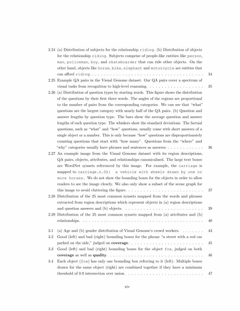
2.24 (a) Distribution of subjects for the relationship riding. (b) Distribution of objects
for the relationship riding. Subjects comprise of people-like entities like person,
man, policeman, boy, and skateboarder that can ride other objects. On the
other hand, objects like horse, bike, elephant and motorcycle are entities that
can afford riding. . . . . . . . . . . . . . . . . . . . . . . . . . . . . . . . . . . . . . 34
2.25 Example QA pairs in the Visual Genome dataset. Our QA pairs cover a spectrum of
visual tasks from recognition to high-level reasoning. . . . . . . . . . . . . . . . . . . 35
2.26 (a) Distribution of question types by starting words. This figure shows the distribution
of the questions by their first three words. The angles of the regions are proportional
to the number of pairs from the corresponding categories. We can see that “what”
questions are the largest category with nearly half of the QA pairs. (b) Question and
answer lengths by question type. The bars show the average question and answer
lengths of each question type. The whiskers show the standard deviations. The factual
questions, such as “what” and “how” questions, usually come with short answers of a
single object or a number. This is only because “how” questions are disproportionately
counting questions that start with “how many”. Questions from the “where” and
“why” categories usually have phrases and sentences as answers. . . . . . . . . . . . . 36
2.27 An example image from the Visual Genome dataset with its region descriptions,
QA pairs, objects, attributes, and relationships canonicalized. The large text boxes
are WordNet synsets referenced by this image. For example, the carriage is
mapped to carriage.n.02: a vehicle with wheels drawn by one or
more horses. We do not show the bounding boxes for the objects in order to allow
readers to see the image clearly. We also only show a subset of the scene graph for
this image to avoid cluttering the figure. . . . . . . . . . . . . . . . . . . . . . . . . . 37
2.28 Distribution of the 25 most common synsets mapped from the words and phrases
extracted from region descriptions which represent objects in (a) region descriptions
and question answers and (b) objects. . . . . . . . . . . . . . . . . . . . . . . . . . . 39
2.29 Distribution of the 25 most common synsets mapped from (a) attributes and (b)
relationships. . . . . . . . . . . . . . . . . . . . . . . . . . . . . . . . . . . . . . . . . 40
3.1 (a) Age and (b) gender distribution of Visual Genome’s crowd workers. . . . . . . . 43
3.2 Good (left) and bad (right) bounding boxes for the phrase “a street with a red car
parked on the side,” judged on coverage. . . . . . . . . . . . . . . . . . . . . . . . . 45
3.3 Good (left) and bad (right) bounding boxes for the object fox, judged on both
coverage as well as quality. . . . . . . . . . . . . . . . . . . . . . . . . . . . . . . . 46
3.4 Each object (fox) has only one bounding box referring to it (left). Multiple boxes
drawn for the same object (right) are combined together if they have a minimum
threshold of 0.9 intersection over union. . . . . . . . . . . . . . . . . . . . . . . . . . 47
xiv
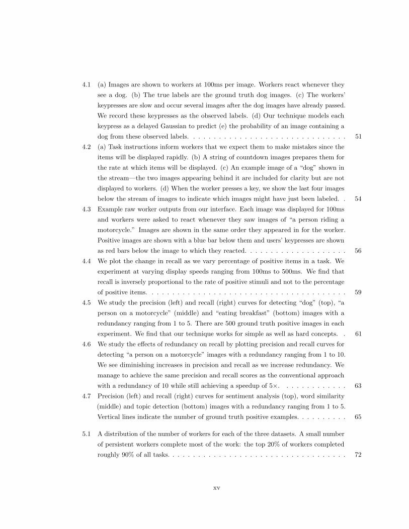
4.1 (a) Images are shown to workers at 100ms per image. Workers react whenever they
see a dog. (b) The true labels are the ground truth dog images. (c) The workers’
keypresses are slow and occur several images after the dog images have already passed.
We record these keypresses as the observed labels. (d) Our technique models each
keypress as a delayed Gaussian to predict (e) the probability of an image containing a
dog from these observed labels. . . . . . . . . . . . . . . . . . . . . . . . . . . . . . . 51
4.2 (a) Task instructions inform workers that we expect them to make mistakes since the
items will be displayed rapidly. (b) A string of countdown images prepares them for
the rate at which items will be displayed. (c) An example image of a “dog” shown in
the stream—the two images appearing behind it are included for clarity but are not
displayed to workers. (d) When the worker presses a key, we show the last four images
below the stream of images to indicate which images might have just been labeled. . 54
4.3 Example raw worker outputs from our interface. Each image was displayed for 100ms
and workers were asked to react whenever they saw images of “a person riding a
motorcycle.” Images are shown in the same order they appeared in for the worker.
Positive images are shown with a blue bar below them and users’ keypresses are shown
as red bars below the image to which they reacted. . . . . . . . . . . . . . . . . . . . 56
4.4 We plot the change in recall as we vary percentage of positive items in a task. We
experiment at varying display speeds ranging from 100ms to 500ms. We find that
recall is inversely proportional to the rate of positive stimuli and not to the percentage
of positive items. . . . . . . . . . . . . . . . . . . . . . . . . . . . . . . . . . . . . . . 59
4.5 We study the precision (left) and recall (right) curves for detecting “dog” (top), “a
person on a motorcycle” (middle) and “eating breakfast” (bottom) images with a
redundancy ranging from 1 to 5. There are 500 ground truth positive images in each
experiment. We find that our technique works for simple as well as hard concepts. . 61
4.6 We study the effects of redundancy on recall by plotting precision and recall curves for
detecting “a person on a motorcycle” images with a redundancy ranging from 1 to 10.
We see diminishing increases in precision and recall as we increase redundancy. We
manage to achieve the same precision and recall scores as the conventional approach
with a redundancy of 10 while still achieving a speedup of 5×. . . . . . . . . . . . . 63
4.7 Precision (left) and recall (right) curves for sentiment analysis (top), word similarity
(middle) and topic detection (bottom) images with a redundancy ranging from 1 to 5.
Vertical lines indicate the number of ground truth positive examples. . . . . . . . . . 65
5.1 A distribution of the number of workers for each of the three datasets. A small number
of persistent workers complete most of the work: the top 20% of workers completed
roughly 90% of all tasks. . . . . . . . . . . . . . . . . . . . . . . . . . . . . . . . . . . 72
xv
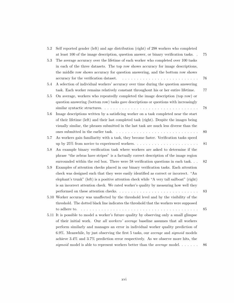
5.2 Self reported gender (left) and age distribution (right) of 298 workers who completed
at least 100 of the image description, question answer, or binary verification tasks. . 75
5.3 The average accuracy over the lifetime of each worker who completed over 100 tasks
in each of the three datasets. The top row shows accuracy for image descriptions,
the middle row shows accuracy for question answering, and the bottom row shows
accuracy for the verification dataset. . . . . . . . . . . . . . . . . . . . . . . . . . . 76
5.4 A selection of individual workers’ accuracy over time during the question answering
task. Each worker remains relatively constant throughout his or her entire lifetime. 77
5.5 On average, workers who repeatedly completed the image description (top row) or
question answering (bottom row) tasks gave descriptions or questions with increasingly
similar syntactic structures. . . . . . . . . . . . . . . . . . . . . . . . . . . . . . . . . 78
5.6 Image descriptions written by a satisficing worker on a task completed near the start
of their lifetime (left) and their last completed task (right). Despite the images being
visually similar, the phrases submitted in the last task are much less diverse than the
ones submitted in the earlier task. . . . . . . . . . . . . . . . . . . . . . . . . . . . . 80
5.7 As workers gain familiarity with a task, they become faster. Verification tasks speed
up by 25% from novice to experienced workers. . . . . . . . . . . . . . . . . . . . . . 81
5.8 An example binary verification task where workers are asked to determine if the
phrase “the zebras have stripes” is a factually correct description of the image region
surrounded within the red box. There were 58 verification questions in each task. . . 82
5.9 Examples of attention checks placed in our binary verification tasks. Each attention
check was designed such that they were easily identified as correct or incorrect. “An
elephant’s trunk” (left) is a positive attention check while “A very tall sailboat” (right)
is an incorrect attention check. We rated worker’s quality by measuring how well they
performed on these attention checks. . . . . . . . . . . . . . . . . . . . . . . . . . . . 83
5.10 Worker accuracy was unaffected by the threshold level and by the visibility of the
threshold. The dotted black line indicates the threshold that the workers were supposed
to adhere to. . . . . . . . . . . . . . . . . . . . . . . . . . . . . . . . . . . . . . . . . 85
5.11 It is possible to model a worker’s future quality by observing only a small glimpse
of their initial work. Our all workers’ average baseline assumes that all workers
perform similarly and manages an error in individual worker quality prediction of
6.9%. Meanwhile, by just observing the first 5 tasks, our average and sigmoid models
achieve 3.4% and 3.7% prediction error respectively. As we observe more hits, the
sigmoid model is able to represent workers better than the average model. . . . . . . 86
xvi
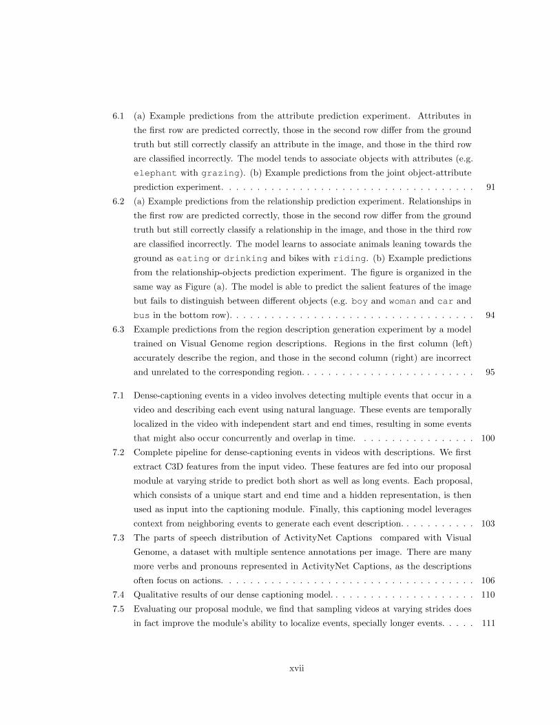
6.1 (a) Example predictions from the attribute prediction experiment. Attributes in
the first row are predicted correctly, those in the second row differ from the ground
truth but still correctly classify an attribute in the image, and those in the third row
are classified incorrectly. The model tends to associate objects with attributes (e.g.
elephant with grazing). (b) Example predictions from the joint object-attribute
prediction experiment. . . . . . . . . . . . . . . . . . . . . . . . . . . . . . . . . . . . 91
6.2 (a) Example predictions from the relationship prediction experiment. Relationships in
the first row are predicted correctly, those in the second row differ from the ground
truth but still correctly classify a relationship in the image, and those in the third row
are classified incorrectly. The model learns to associate animals leaning towards the
ground as eating or drinking and bikes with riding. (b) Example predictions
from the relationship-objects prediction experiment. The figure is organized in the
same way as Figure (a). The model is able to predict the salient features of the image
but fails to distinguish between different objects (e.g. boy and woman and car and
bus in the bottom row). . . . . . . . . . . . . . . . . . . . . . . . . . . . . . . . . . . 94
6.3 Example predictions from the region description generation experiment by a model
trained on Visual Genome region descriptions. Regions in the first column (left)
accurately describe the region, and those in the second column (right) are incorrect
and unrelated to the corresponding region. . . . . . . . . . . . . . . . . . . . . . . . . 95
7.1 Dense-captioning events in a video involves detecting multiple events that occur in a
video and describing each event using natural language. These events are temporally
localized in the video with independent start and end times, resulting in some events
that might also occur concurrently and overlap in time. . . . . . . . . . . . . . . . . 100
7.2 Complete pipeline for dense-captioning events in videos with descriptions. We first
extract C3D features from the input video. These features are fed into our proposal
module at varying stride to predict both short as well as long events. Each proposal,
which consists of a unique start and end time and a hidden representation, is then
used as input into the captioning module. Finally, this captioning model leverages
context from neighboring events to generate each event description. . . . . . . . . . . 103
7.3 The parts of speech distribution of ActivityNet Captions compared with Visual
Genome, a dataset with multiple sentence annotations per image. There are many
more verbs and pronouns represented in ActivityNet Captions, as the descriptions
often focus on actions. . . . . . . . . . . . . . . . . . . . . . . . . . . . . . . . . . . . 106
7.4 Qualitative results of our dense captioning model. . . . . . . . . . . . . . . . . . . . . 110
7.5 Evaluating our proposal module, we find that sampling videos at varying strides does
in fact improve the module’s ability to localize events, specially longer events. . . . . 111
xvii
7.6 (a) The number of sentences within paragraphs is normally distributed, with on
average 3.65 sentences per paragraph. (b) The number of words per sentence within
paragraphs is normally distributed, with on average 13.48 words per sentence. . . . . 114
7.7 Distribution of number of sentences with respect to video length. In general the longer
the video the more sentences there are, so far on average each additional minute adds
one more sentence to the paragraph. . . . . . . . . . . . . . . . . . . . . . . . . . . . 116
7.8 Distribution of annotations in time in ActivityNet Captions videos, most of the
annotated time intervals are closer to the middle of the videos than to the start and end.117
7.9 (a) The most frequently used words in ActivityNet Captions with stop words removed.
(b) The most frequently used bigrams in ActivityNet Captions . . . . . . . . . . . . . 117
7.10 (a) Interface when a worker is writing a paragraph. Workers are asked to write a
paragraph in the text box and press ”Done Writing Paragraph” before they can
proceed with grounding each of the sentences. (b) Interface when labeling sentences
with start and end timestamps. Workers select each sentence, adjust the range slider
indicating which segment of the video that particular sentence is referring to. They
then click save and proceed to the next sentence. (c) We show examples of good and
bad annotations to workers. Each task contains one good and one bad example video
with annotations. We also explain why the examples are considered to be good or bad.118
7.11 More qualitative dense-captioning captions generated using our model. We show
captions with the highest overlap with ground truth captions. . . . . . . . . . . . . . 119
7.12 The number of videos (red) corresponding to each ActivityNet class label, as well
as the number of videos (blue) that has the label appearing in their ActivityNet
Captions paragraph descriptions. . . . . . . . . . . . . . . . . . . . . . . . . . . . . . 120
xviii
Chapter 1
Introduction
1.1 Motivation
Despite recent breakthroughs in solving perceptual tasks like image classification, modern computer
vision models are still unable to perform well on reasoning tasks such as captioning a scene or
answering questions. A potential reason for the performance gap is that current computer vision
models are often trained on traditional, large-scale datasets created for perceptual tasks. Therefore,
as the complexity for problems in computer vision rises, so does the need for the creation and use of
new, richer large-scale datasets.
Interesting problems in both human-computer interaction and computer vision arise in the creation
of these datasets. For example, better understanding the crowdsourcing processes common in the
creation of modern datasets may help reduce costs while simultaneously improving the quality of the
data collected. Additionally, new methods for automating many parts of a crowdsourcing pipeline
may leverage modern computer vision techniques.
Ultimately, the main goal of this thesis is two-fold. First, we want to understand and improve the
crowdsourcing pipeline for collecting large-scale visual datasets. Second, we want to demonstrate
how we can use these new computer vision datasets to build models that can better tackle more
complex reasoning tasks.
1.2 Thesis Outline
In this thesis, we first focus on the theme of understanding the entire process of building computer
vision models that leverage large-scale data. In Chapter 2, we introduce Visual Genome, the densest
crowdsourced dataset for large-scale visual content. The concepts of connecting objects, attributes,
and relationships within each image enable us to build scene graphs of images and form the densest
database for visual knowledge representation. Chapter 3 covers the main crowdsourcing pipeline
1
CHAPTER 1. INTRODUCTION 2
we used to collect the Visual Genome dataset. We outline the lessons learned to transfer common
strategies that may be employed in the collection of other computer vision or natural language
processing datasets. Chapter 4 dives into a novel crowdsourcing method that models worker latency
to rapidly collect binary labels for large-scale datasets like Visual Genome. This approach leads to an
order of magnitude speedup in crowdwork, leading to significant cost reductions. Chapter 5 studies
how we can use the collection of large datasets to better understand crowd workers at scale. We find
that crowd workers maintain a consistent quality level during the completion of microtasks, allowing
for dataset creators to easily ascertain good crowd workers early on. Chapter 6 discusses how we can
leverage Visual Genome to solve new tasks in computer vision. Chapter 7 focuses on the collection
and use of a new, large-scale video dataset in order to densely caption videos with sentences. In this
chapter, we illustrate the complexity of tasks that can be achieved with the construction of new
datasets with new computer vision models. Finally, Chapter 8 provides a brief summary of the future
directions and applications of the research discussed.
1.3 Previously Published Papers
The majority of contributions of this thesis has previously appeared in various publications: [118]
(Chapters 2 and 3), [119] (Chapter 4), [81] (Chapter 5), [117] (Chapter 6). Other publications [228]
are out of context with the theme of this thesis and consequently are not included.
Chapter 2
Visual Genome
2.1 Introduction
A holy grail of computer vision is the complete understanding of visual scenes: a model that
is able to name and detect objects, describe their attributes, and recognize their relationships.
Understanding scenes would enable important applications such as image search, question answering,
and robotic interactions. Much progress has been made in recent years towards this goal, including
image classification [180, 219, 120, 231] and object detection [71, 212, 70, 190]. An important
contributing factor is the availability of a large amount of data that drives the statistical models that
underpin today’s advances in computational visual understanding. While the progress is exciting,
we are still far from reaching the goal of comprehensive scene understanding. As Figure 2.1 shows,
existing models would be able to detect discrete objects in a photo but would not be able to explain
their interactions or the relationships between them. Such explanations tend to be cognitive in
nature, integrating perceptual information into conclusions about the relationships between objects
in a scene [19, 63]. A cognitive understanding of our visual world thus requires that we complement
computers’ ability to detect objects with abilities to describe those objects [97] and understand their
interactions within a scene [204].
There is an increasing effort to put together the next generation of datasets to serve as training
and benchmarking datasets for these deeper, cognitive scene understanding and reasoning tasks,
the most notable being MS-COCO [140] and VQA [2]. The MS-COCO dataset consists of 300K
real-world photos collected from Flickr. For each image, there is pixel-level segmentation of 80 object
classes (when present) and 5 independent, user-generated sentences describing the scene. VQA adds
Visual Genome was a highly collaborative project between many students, faculty, and industry affiliates. Mymain contributions to the Visual Genome project involved helping build the crowdsourcing framework, benchmarkingthe dataset with deep neural networks, and then iterating on the dataset to be usable for computer vision researchers.
3
CHAPTER 2. VISUAL GENOME 4
Figure 2.1: An overview of the data needed to move from perceptual awareness to cognitiveunderstanding of images. We present a dataset of images densely annotated with numerous regiondescriptions, objects, attributes, and relationships. Some examples of region descriptions (e.g. “girlfeeding large elephant” and “a man taking a picture behind girl”) are shown (top). The objects (e.g.elephant), attributes (e.g. large) and relationships (e.g. feeding) are shown (bottom). Ourdataset also contains image related question answer pairs (not shown).
to this a set of 614K question answer pairs related to the visual contents of each image (see more
details in Section 2.2.1). With this information, MS-COCO and VQA provide a fertile training
and testing ground for models aimed at tasks for accurate object detection, segmentation, and
summary-level image captioning [111, 150, 109]as well as basic QA [189, 147, 66, 146]. For example,
a state-of-the-art model [109] provides a description of one MS-COCO image in Figure 2.1 as “two
men are standing next to an elephant.” But what is missing is the further understanding of where
each object is, what each person is doing, what the relationship between the person and elephant is,
etc. Without such relationships, these models fail to differentiate this image from other images of
people next to elephants.
To understand images thoroughly, we believe three key elements need to be added to existing
datasets: a grounding of visual concepts to language [111], a more complete set of de-
scriptions and QAs for each image based on multiple image regions [102], and a formalized
representation of the components of an image [82]. In the spirit of mapping out this complete
information of the visual world, we introduce the Visual Genome dataset. The first release of the
Visual Genome dataset uses 108, 077 images from the intersection of the YFCC100M [234] and
MS-COCO [140]. Section 2.4 provides a more detailed description of the dataset. We highlight
below the motivation and contributions of the three key elements that set Visual Genome apart from
existing datasets.
The Visual Genome dataset regards relationships and attributes as first-class citizens of the
annotation space, in addition to the traditional focus on objects. Recognition of relationships and
attributes is an important part of the complete understanding of the visual scene, and in many cases,
CHAPTER 2. VISUAL GENOME 5
these elements are key to the story of a scene (e.g., the difference between “a dog chasing a man”
versus “a man chasing a dog”). The Visual Genome dataset is among the first to provide a detailed
labeling of object interactions and attributes, grounding visual concepts to language1
An image is often a rich scenery that cannot be fully described in one summarizing sentence. The
scene in Figure 2.1 contains multiple “stories”: “a man taking a photo of elephants,” “a woman
feeding an elephant,” “a river in the background of lush grounds,” etc. Existing datasets such as
Flickr 30K [275] and MS-COCO [140] focus on high-level descriptions of an image2. Instead, for each
image in the Visual Genome dataset, we collect more than 50 descriptions for different regions in
the image, providing a much denser and more complete set of descriptions of the scene. In
addition, inspired by VQA [2], we also collect an average of 17 question answer pairs based on the
descriptions for each image. Region-based question answers can be used to jointly develop NLP and
vision models that can answer questions from either the description or the image, or both of them.
With a set of dense descriptions of an image and the explicit correspondences between visual
pixels (i.e. bounding boxes of objects) and textual descriptors (i.e. relationships, attributes), the
Visual Genome dataset is poised to be the first image dataset that is capable of providing a
structured formalized representation of an image, in the form that is widely used in knowledge
base representations in NLP [281, 77, 38, 223]. For example, in Figure 2.1, we can formally express
the relationship holding between the woman and food as holding(woman, food)). Putting together
all the objects and relations in a scene, we can represent each image as a scene graph [102]. The
scene graph representation has been shown to improve semantic image retrieval [102, 210] and image
captioning [57, 28, 78]. Furthermore, all objects, attributes and relationships in each image in the
Visual Genome dataset are canonicalized to its corresponding WordNet [160] ID (called a synset ID).
This mapping connects all images in Visual Genome and provides an effective way to consistently
query the same concept (object, attribute, or relationship) in the dataset. It can also potentially
help train models that can learn from contextual information from multiple images.
In this paper, we introduce the Visual Genome dataset3 with the aim of training and benchmarking
the next generation of computer models for comprehensive scene understanding. The paper proceeds
as follows: In Section 2.3, we provide a detailed description of each component of the dataset.
Section 2.2 provides a literature review of related datasets as well as related recognition tasks.
Section 3 discusses the crowdsourcing strategies we deployed in the ongoing effort of collecting this
dataset. Section 2.4 is a collection of data analysis statistics, showcasing the key properties of the
Visual Genome dataset. Last but not least, Section 6.1 provides a set of experimental results that
use Visual Genome as a benchmark.
1The Lotus Hill Dataset [271] also provides a similar annotation of object relationships, see Sec 2.2.1.2COCO has multiple sentences generated independently by different users, all focusing on providing an overall, one
sentence description of the scene.3Further visualizations, API, and additional information on the Visual Genome dataset can be found online: https:
//visualgenome.org
CHAPTER 2. VISUAL GENOME 6
The man is almost bald
Park bench is made of gray weathered wood
A man and a woman sit on a park bench along a river.
Figure 2.2: An example image from the Visual Genome dataset. We show 3 region descriptions andtheir corresponding region graphs. We also show the connected scene graph collected by combiningall of the image’s region graphs. The top region description is “a man and a woman sit on a parkbench along a river.” It contains the objects: man, woman, bench and river. The relationshipsthat connect these objects are: sits on(man, bench), in front of (man, river), and sits on(woman,bench).
CHAPTER 2. VISUAL GENOME 7
Figure 2.3: An example image from our dataset along with its scene graph representation. Thescene graph contains objects (child, instructor, helmet, etc.) that are localized in the imageas bounding boxes (not shown). These objects also have attributes: large, green, behind,etc. Finally, objects are connected to each other through relationships: wears(child, helmet),wears(instructor, jacket), etc.
CHAPTER 2. VISUAL GENOME 8
Que
stio
nsR
egio
n D
escr
iptio
nsR
egio
n G
raph
sS
cene
Gra
ph
Legend: objects relationshipsattributes
fire hydrant
yellow
fire hydrant
man
woman
standing
jumping over
man shorts
inis behind
fire hydrant
man
jumping over
woman
standingshorts
in
is behind
yellow
woman in shorts is standing behind the man
yellow fire hydrant
Q. What is the woman standing next to?
A. Her belongings.
Q. What color is the fire hydrant?
A. Yellow.
man jumping over fire hydrant
Region Based Question Answers Free Form Question Answers
Figure 2.4: A representation of the Visual Genome dataset. Each image contains region descriptionsthat describe a localized portion of the image. We collect two types of question answer pairs (QAs):freeform QAs and region-based QAs. Each region is converted to a region graph representation ofobjects, attributes, and pairwise relationships. Finally, each of these region graphs are combined toform a scene graph with all the objects grounded to the image. Best viewed in color
CHAPTER 2. VISUAL GENOME 9
2.2 Related Work
We discuss existing datasets that have been released and used by the vision community for classification
and object detection. We also mention work that has improved object and attribute detection models.
Then, we explore existing work that has utilized representations similar to our relationships between
objects. In addition, we dive into literature related to cognitive tasks like image description, question
answering, and knowledge representation.
2.2.1 Datasets
Datasets (Table 2.1) have been growing in size as researchers have begun tackling increasingly
complicated problems. Caltech 101 [59] was one of the first datasets hand-curated for image
classification, with 101 object categories and 15-30 examples per category. One of the biggest
criticisms of Caltech 101 was the lack of variability in its examples. Caltech 256 [76] increased
the number of categories to 256, while also addressing some of the shortcomings of Caltech 101.
However, it still had only a handful of examples per category, and most of its images contained only
a single object. LabelMe [201] introduced a dataset with multiple objects per category. They also
provided a web interface that experts and novices could use to annotate additional images. This web
interface enabled images to be labeled with polygons, helping create datasets for image segmentation.
The Lotus Hill dataset [271] contains a hierarchical decomposition of objects (vehicles, man-made
objects, animals, etc.) along with segmentations. Only a small part of this dataset is freely available.
SUN [261], just like LabelMe [201] and Lotus Hill [271], was curated for object detection. Pushing the
size of datasets even further, 80 Million Tiny Images [238] created a significantly larger dataset than
its predecessors. It contains tiny (i.e. 32× 32 pixels) images that were collected using WordNet [160]
synsets as queries. However, because the data in 80 Million Images were not human-verified, they
contain numerous errors. YFCC100M [234] is another large database of 100 million images that is
still largely unexplored. It contains human generated and machine generated tags.
Pascal VOC [54] pushed research from classification to object detection with a dataset containing
20 semantic categories in 11, 000 images. ImageNet [43] took WordNet synsets and crowdsourced
a large dataset of 14 million images. They started the ILSVRC [198] challenge for a variety of
computer vision tasks. Together, ILSVRC and PASCAL provide a test bench for object detection,
image classification, object segmentation, person layout, and action classification. MS-COCO [140]
recently released its dataset, with over 328, 000 images with sentence descriptions and segmentations
of 80 object categories. The previous largest dataset for image-based QA, VQA [2], contains 204, 721
images annotated with three question answer pairs. They collected a dataset of 614, 163 freeform
questions with 6.1M ground truth answers (10 per question) and provided a baseline approach in
answering questions using an image and a textual question as the input.
Visual Genome aims to bridge the gap between all these datasets, collecting not just annotations

CHAPTER 2. VISUAL GENOME 10
Descriptions
Tota
l#
Object
Objects
#Attributes
Attributes
#Rel.
Rel.
Question
Images
perIm
age
Objects
Categories
perIm
age
Categories
perIm
age
Categories
perIm
age
Answ
ers
YFCC100M
[234]
100,000,000
--
--
--
--
-
TinyIm
ages[238]
80,000,000
--
53,464
1-
--
--
ImageNet[43]
14,197,122
-14,197,122
21,841
1-
--
--
ILSVRC
[198]
476,688
-534,309
200
2.5
--
--
-
MS-C
OCO
[140]
328,000
527,472
80
--
--
--
Flick
r30K
[275]
31,783
5-
--
--
--
-
Caltech
101[59]
9,144
-9,144
102
1-
--
--
Caltech
256[76]
30,608
-30,608
257
1-
--
--
Caltech
Ped.[48]
250,000
-350,000
11.4
--
--
-
PascalDetection
[54]
11,530
-27,450
20
2.38
--
--
-
Abstra
ctScenes[285]
10,020
-58
11
5-
--
--
aPascal[57]
12,000
--
--
64
--
--
AwA
[126]
30,000
--
--
1,280
--
--
SUN
Attributes[177]
14,000
--
--
700
700
--
-
Caltech
Birds[250]
11,788
--
--
312
312
--
-
COCO
Actions[195]
10,000
--
-5.2
--
156
20.7
-
VisualPhra
ses[204]
--
--
--
-17
1-
VisKE
[203]
--
--
--
-6500
--
DAQUAR
[146]
1,449
--
--
--
--
12,468
COCO
QA
[189]
123,287
--
--
--
--
117,684
Baidu
[66]
120,360
--
--
--
--
250,569
VQA
[2]
204,721
--
--
--
--
614,163
VisualG
enom
e108,077
50
3,843,636
33,877
35
68,111
26
42,374
21
1,773,258
Table
2.1
:A
com
pari
son
of
exis
ting
data
sets
wit
hV
isual
Gen
om
e.W
esh
owth
at
Vis
ual
Gen
om
ehas
an
ord
erof
magnit
ude
more
des
crip
tions
and
ques
tion
answ
ers.
Itals
ohas
am
ore
div
erse
set
of
ob
ject
,att
ribute
,and
rela
tionsh
ipcl
ass
es.
Addit
ionally,
Vis
ual
Gen
ome
conta
ins
ah
igh
erd
ensi
tyof
thes
ean
not
atio
ns
per
imag
e.T
he
nu
mb
erof
dis
tin
ctca
tego
ries
inV
isual
Gen
ome
are
calc
ula
ted
by
low
er-c
asin
gan
dst
emm
ing
nam
esof
obje
cts,
att
rib
ute
san
dre
lati
on
ship
s.
CHAPTER 2. VISUAL GENOME 11
for a large number of objects but also scene graphs, region descriptions, and question answer pairs for
image regions. Unlike previous datasets, which were collected for a single task like image classification,
the Visual Genome dataset was collected to be a general-purpose representation of the visual world,
without bias toward a particular task. Our images contain an average of 35 objects, which is almost
an order of magnitude more dense than any existing vision dataset. Similarly, we contain an average
of 26 attributes and 21 relationships per image. We also have an order of magnitude more unique
objects, attributes, and relationships than any other dataset. Finally, we have 1.7 million question
answer pairs, also larger than any other dataset for visual question answering.
2.2.2 Image Descriptions
One of the core contributions of Visual Genome is its descriptions for multiple regions in an image.
As such, we mention other image description datasets and models in this subsection. Most work
related to describing images can be divided into two categories: retrieval of human-generated captions
and generation of novel captions. Methods in the first category use similarity metrics between image
features from predefined models to retrieve similar sentences [170, 90]. Other methods map both
sentences and their images to a common vector space [170] or map them to a space of triples [56].
Among those in the second category, a common theme has been to use recurrent neural networks to
produce novel captions [111, 150, 109, 247, 31, 49, 55]. More recently, researchers have also used a
visual attention model [264].
One drawback of these approaches is their attention to describing only the most salient aspect of
the image. This problem is amplified by datasets like Flickr 30K [275] and MS-COCO [140], whose
sentence desriptions tend to focus, somewhat redundantly, on these salient parts. For example, “an
elephant is seen wandering around on a sunny day,” “a large elephant in a tall grass field,” and “a
very large elephant standing alone in some brush” are 3 descriptions from the MS-COCO dataset,
and all of them focus on the salient elephant in the image and ignore the other regions in the image.
Many real-world scenes are complex, with multiple objects and interactions that are best described
using multiple descriptions [109, 135]. Our dataset pushes toward a more complete understanding
of an image by collecting a dataset in which we capture not just scene-level descriptions but also
myriad of low-level descriptions, the “grammar” of the scene.
2.2.3 Objects
Object detection is a fundamental task in computer vision, with applications ranging from identi-
fication of faces in photo software to identification of other cars by self-driving cars on the road.
It involves classifying an object into a distinct category and localizing the object in the image.
Visual Genome uses objects as a core component on which each visual scene is built. Early datasets
include the face detection [92] and pedestrian datasets [48]. The PASCAL VOC and ILSVRC’s
detection dataset pushed research in object detection. But the images in these datasets are iconic
CHAPTER 2. VISUAL GENOME 12
and do not capture the settings in which these objects usually co-occur. To remedy this problem,
MS-COCO [140] annotated real-world scenes that capture object contexts. However, MS-COCO was
unable to describe all the objects in its images, since they annotated only 80 object categories. In
the real world, there are many more objects that the ones captured by existing datasets. Visual
Genome aims at collecting annotations for all visual elements that occur in images, increasing the
number of distinct categories to 33, 877.
2.2.4 Attributes
The inclusion of attributes allows us to describe, compare, and more easily categorize objects. Even
if we haven’t seen an object before, attributes allow us to infer something about it; for example,
“yellow and brown spotted with long neck” likely refers to a giraffe. Initial work in this area involved
finding objects with similar features [148] using examplar SVMs. Next, textures were used to study
objects [241], while other methods learned to predict colors [61]. Finally, the study of attributes was
explicitly demonstrated to lead to improvements in object classification [57]. Attributes were defined
to be parts (e.g. “has legs”), shapes (e.g. “spherical”), or materials (e.g. “furry”) and could be used to
classify new categories of objects. Attributes have also played a large role in improving fine-grained
recognition [73] on fine-grained attribute datasets like CUB-2011 [250]. In Visual Genome, we use a
generalized formulation [102], but we extend it such that attributes are not image-specific binaries
but rather object-specific for each object in a real-world scene. We also extend the types of attributes
to include size (e.g. “small”), pose (e.g. “bent”), state (e.g. “transparent”), emotion (e.g. “happy”),
and many more.
2.2.5 Relationships
Relationship extraction has been a traditional problem in information extraction and in natural
language processing. Syntactic features [281, 77], dependency tree methods [38, 20], and deep neural
networks [223, 278] have been employed to extract relationships between two entities in a sentence.
However, in computer vision, very little work has gone into learning or predicting relationships.
Instead, relationships have been implicitly used to improve other vision tasks. Relative layouts
between objects have improved scene categorization [98], and 3D spatial geometry between objects
has helped object detection [36]. Comparative adjectives and prepositions between pairs of objects
have been used to model visual relationships and improved object localization [78].
Relationships have already shown their utility in improving visual cognitive tasks [3, 269]. A
meaning space of relationships has improved the mapping of images to sentences [56]. Relationships
in a structured representation with objects have been defined as a graph structure called a scene
graph, where the nodes are objects with attributes and edges are relationships between objects. This
representation can be used to generate indoor images from sentences and also to improve image
search [28, 102]. We use a similar scene graph representation of an image that generalizes across all
CHAPTER 2. VISUAL GENOME 13
these previous works [102]. Recently, relationships have come into focus again in the form of question
answering about associations between objects [203]. These questions ask if a relationship, involving
generally two objects, is true, e.g. “do dogs eat ice cream?”. We believe that relationships will be
necessary for higher-level cognitive tasks [102, 144], so we collect the largest corpus of them in an
attempt to improve tasks by actually understanding interactions between objects.
2.2.6 Question Answering
Visual question answering (QA) has been recently proposed as a proxy task of evaluating a computer
vision system’s ability to understand an image beyond object recognition and image captioning [68,
146]. Several visual QA benchmarks have been proposed in the last few months. The DAQUAR [146]
dataset was the first toy-sized QA benchmark built upon indoor scene RGB-D images of NYU Depth
v2 [163]. Most new datasets [277, 189, 2, 66] have collected QA pairs on MS-COCO images, either
generated automatically by NLP tools [189] or written by human workers [277, 2, 66].
In previous datasets, most questions concentrated on simple recognition-based questions about the
salient objects, and answers were often extremely short. For instance, 90% of DAQUAR answers [146]
and 89% of VQA answers [2] consist of single-word object names, attributes, and quantities. This
limitation bounds their diversity and fails to capture the long-tail details of the images. Given the
availability of new datasets, an array of visual QA models have been proposed to tackle QA tasks.
The proposed models range from SVM classifiers and probabilistic inference [146] to recurrent neural
networks [66, 147, 189] and convolutional networks [145]. Visual Genome aims to capture the details
of the images with diverse question types and long answers. These questions should cover a wide
range of visual tasks from basic perception to complex reasoning. Our QA dataset of 1.7 million
QAs is also larger than any currently existing dataset.
2.2.7 Knowledge Representation
A knowledge representation of the visual world is capable of tackling an array of vision tasks, from
action recognition to general question answering. However, it is difficult to answer “what is the
minimal viable set of knowledge needed to understand about the physical world?” [82]. It was
later proposed that there be a certain plurality to concepts and their related axioms [83]. These
efforts have grown to model physical processes [64] or to model a series of actions as scripts [206] for
stories—both of which are not depicted in a single static image but which play roles in an image’s
story [243]. More recently, NELL [9] learns probabilistic horn clauses by extracting information
from the web. DeepQA [62] proposes a probabilistic question answering architecture involving over
100 different techniques. Others have used Markov logic networks [282, 167] as their representation
to perform statistical inference for knowledge base construction. Our work is most similar to that
of those [32, 283, 284, 203] who attempt to learn common-sense relationships from images. Visual
CHAPTER 2. VISUAL GENOME 14
Figure 2.5: To describe all the contents of and interactions in an image, the Visual Genome datasetincludes multiple human-generated image regions descriptions, with each region localized by abounding box. Here, we show three regions descriptions on various image regions: “man jumpingover a fire hydrant,” “yellow fire hydrant,” and “woman in shorts is standing behind the man.”
Genome scene graphs can also be considered a dense knowledge representation for images. It is
similar to the format used in knowledge bases in NLP.
2.3 Visual Genome Data Representation
The Visual Genome dataset consists of seven main components: region descriptions, objects, attributes,
relationships, region graphs, scene graphs, and question answer pairs. Figure 2.4 shows examples of
each component for one image. To enable research on comprehensive understanding of images, we
begin by collecting descriptions and question answers. These are raw texts without any restrictions
on length or vocabulary. Next, we extract objects, attributes and relationships from our descriptions.
Together, objects, attributes and relationships comprise our scene graphs that represent a formal
representation of an image. In this section, we break down Figure 2.4 and explain each of the seven
components. In Section 3, we will describe in more detail how data from each component is collected
through a crowdsourcing platform.
2.3.1 Multiple regions and their descriptions
In a real-world image, one simple summary sentence is often insufficient to describe all the contents
of and interactions in an image. Instead, one natural way to extend this might be a collection of
descriptions based on different regions of a scene. In Visual Genome, we collect diverse human-
generated image region descriptions, with each region localized by a bounding box. In Figure 2.5, we
show three examples of region descriptions. Regions are allowed to have a high degree of overlap
CHAPTER 2. VISUAL GENOME 15
Figure 2.6: From all of the region descriptions, we extract all objects mentioned. For example, fromthe region description “man jumping over a fire hydrant,” we extract man and fire hydrant.
with each other when the descriptions differ. For example, “yellow fire hydrant” and “woman in
shorts is standing behind the man” have very little overlap, while “man jumping over fire hydrant”
has a very high overlap with the other two regions. Our dataset contains on average a total of 50
region descriptions per image. Each description is a phrase ranging from 1 to 16 words in length
describing that region.
2.3.2 Multiple objects and their bounding boxes
Each image in our dataset consists of an average of 35 objects, each delineated by a tight bounding
box (Figure 2.6). Furthermore, each object is canonicalized to a synset ID in WordNet [160]. For
example, man would get mapped to man.n.03 (the generic use of the word to refer
to any human being). Similarly, person gets mapped to person.n.01 (a human being).
Afterwards, these two concepts can be joined to person.n.01 since this is a hypernym of man.n.03.
We did not standardize synsets in our dataset. However, given our canonicalization, this is easily
possible leveraging the WordNet ontology to avoid multiple names for one object (e.g. man, person,
human), and to connect information across images.
2.3.3 A set of attributes
Each image in Visual Genome has an average of 26 attributes. Objects can have zero or more attributes
associated with them. Attributes can be color (e.g. yellow), states (e.g. standing), etc. (Fig-
ure 2.7). Just like we collect objects from region descriptions, we also collect the attributes attached to
these objects. In Figure 2.7, from the phrase “yellow fire hydrant,” we extract the attribute yellow
for the fire hydrant. As with objects, we canonicalize all attributes to WordNet [160]; for example,
CHAPTER 2. VISUAL GENOME 16
Figure 2.7: Some descriptions also provide attributes for objects. For example, the region description“yellow fire hydrant” adds that the fire hydrant is yellow. Here we show two attributes: yellowand standing.
yellow is mapped to yellow.s.01 (of the color intermediate between green and
orange in the color spectrum; of something resembling the color of an egg
yolk).
2.3.4 A set of relationships
Relationships connect two objects together. These relationships can be actions (e.g. jumping over),
spatial (e.g. is behind), descriptive verbs (e.g. wear), prepositions (e.g. with), comparative (e.g.
taller than), or prepositional phrases (e.g. drive on). For example, from the region description
“man jumping over fire hydrant,” we extract the relationship jumping over between the objects
man and fire hydrant (Figure 2.8). These relationships are directed from one object, called
the subject, to another, called the object. In this case, the subject is the man, who is performing
the relationship jumping over on the object fire hydrant. Each relationship is canonicalized
to a WordNet [160] synset ID; i.e. jumping is canonicalized to jump.a.1 (move forward by
leaps and bounds). On average, each image in our dataset contains 21 relationships.
2.3.5 A set of region graphs
Combining the objects, attributes, and relationships extracted from region descriptions, we create
a directed graph representation for each of the regions. Examples of region graphs are shown in
Figure 2.4. Each region graph is a structured representation of a part of the image. The nodes in the
graph represent objects, attributes, and relationships. Objects are linked to their respective attributes
while relationships link one object to another. The links connecting two objects in Figure 2.4 point
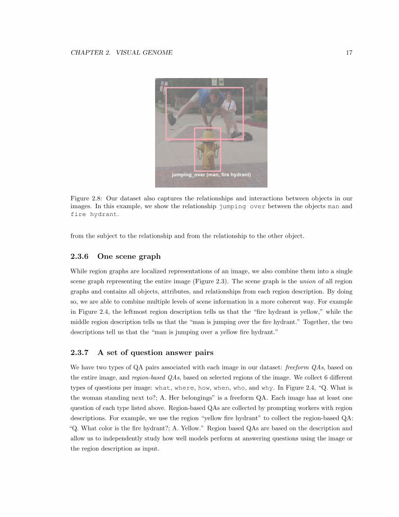
CHAPTER 2. VISUAL GENOME 17
Figure 2.8: Our dataset also captures the relationships and interactions between objects in ourimages. In this example, we show the relationship jumping over between the objects man andfire hydrant.
from the subject to the relationship and from the relationship to the other object.
2.3.6 One scene graph
While region graphs are localized representations of an image, we also combine them into a single
scene graph representing the entire image (Figure 2.3). The scene graph is the union of all region
graphs and contains all objects, attributes, and relationships from each region description. By doing
so, we are able to combine multiple levels of scene information in a more coherent way. For example
in Figure 2.4, the leftmost region description tells us that the “fire hydrant is yellow,” while the
middle region description tells us that the “man is jumping over the fire hydrant.” Together, the two
descriptions tell us that the “man is jumping over a yellow fire hydrant.”
2.3.7 A set of question answer pairs
We have two types of QA pairs associated with each image in our dataset: freeform QAs, based on
the entire image, and region-based QAs, based on selected regions of the image. We collect 6 different
types of questions per image: what, where, how, when, who, and why. In Figure 2.4, “Q. What is
the woman standing next to?; A. Her belongings” is a freeform QA. Each image has at least one
question of each type listed above. Region-based QAs are collected by prompting workers with region
descriptions. For example, we use the region “yellow fire hydrant” to collect the region-based QA:
“Q. What color is the fire hydrant?; A. Yellow.” Region based QAs are based on the description and
allow us to independently study how well models perform at answering questions using the image or
the region description as input.
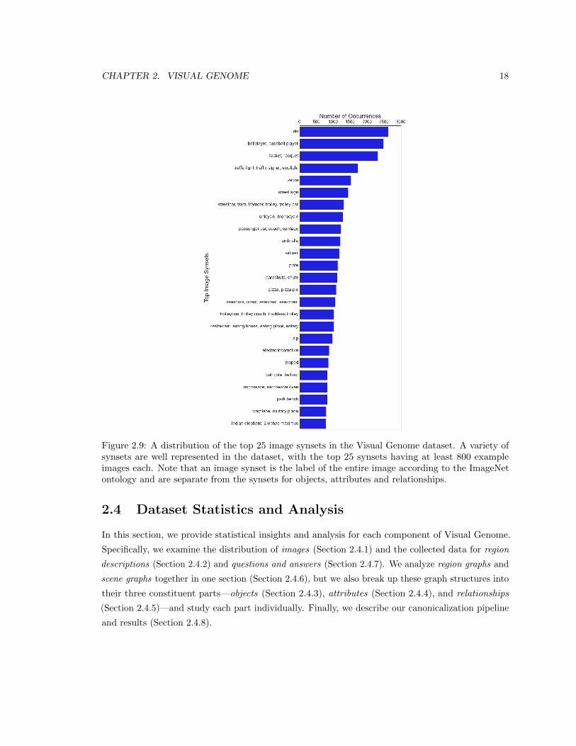
CHAPTER 2. VISUAL GENOME 18
Figure 2.9: A distribution of the top 25 image synsets in the Visual Genome dataset. A variety ofsynsets are well represented in the dataset, with the top 25 synsets having at least 800 exampleimages each. Note that an image synset is the label of the entire image according to the ImageNetontology and are separate from the synsets for objects, attributes and relationships.
2.4 Dataset Statistics and Analysis
In this section, we provide statistical insights and analysis for each component of Visual Genome.
Specifically, we examine the distribution of images (Section 2.4.1) and the collected data for region
descriptions (Section 2.4.2) and questions and answers (Section 2.4.7). We analyze region graphs and
scene graphs together in one section (Section 2.4.6), but we also break up these graph structures into
their three constituent parts—objects (Section 2.4.3), attributes (Section 2.4.4), and relationships
(Section 2.4.5)—and study each part individually. Finally, we describe our canonicalization pipeline
and results (Section 2.4.8).
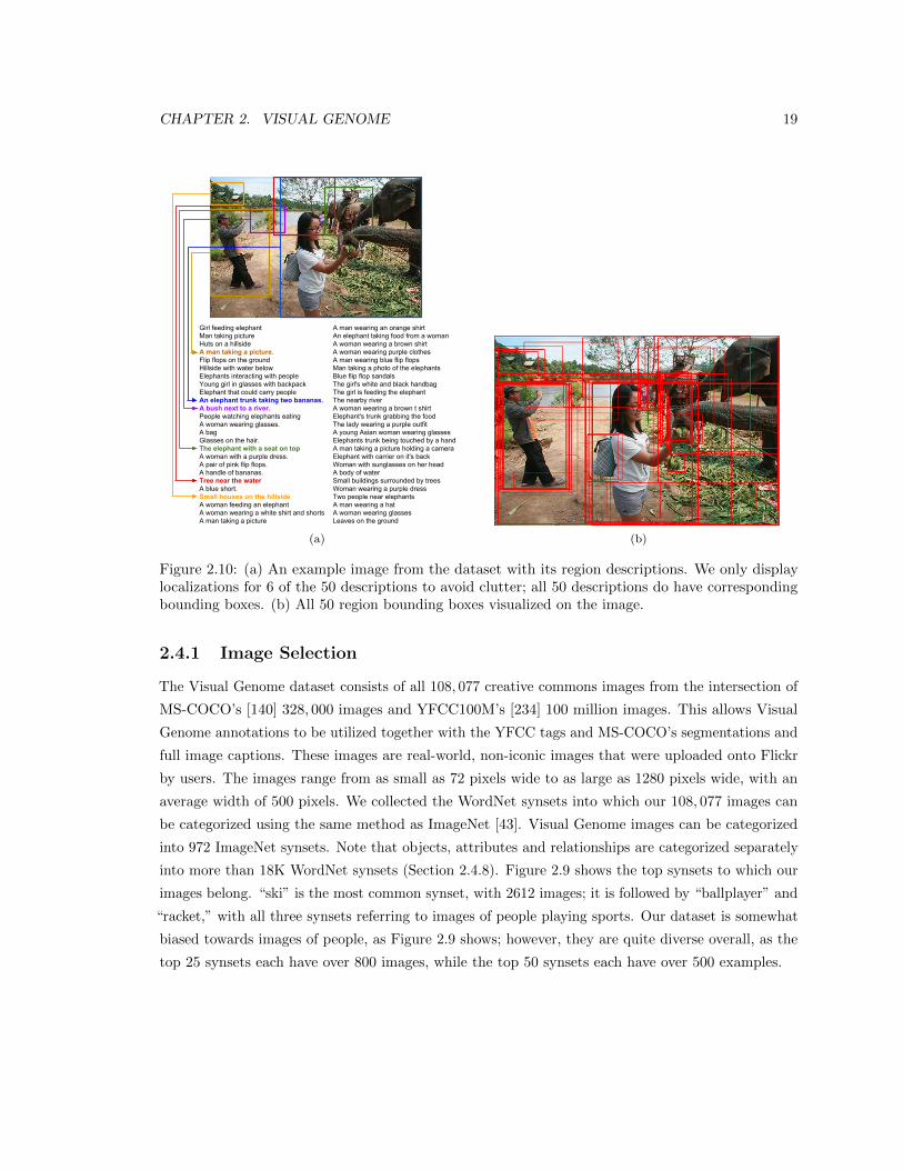
CHAPTER 2. VISUAL GENOME 19
Girl feeding elephantMan taking pictureHuts on a hillsideA man taking a picture.Flip flops on the groundHillside with water belowElephants interacting with peopleYoung girl in glasses with backpackElephant that could carry peopleAn elephant trunk taking two bananas.A bush next to a river.People watching elephants eatingA woman wearing glasses.A bagGlasses on the hair.The elephant with a seat on topA woman with a purple dress.A pair of pink flip flops.A handle of bananas.Tree near the waterA blue short.Small houses on the hillsideA woman feeding an elephantA woman wearing a white shirt and shortsA man taking a picture
A man wearing an orange shirtAn elephant taking food from a womanA woman wearing a brown shirtA woman wearing purple clothesA man wearing blue flip flopsMan taking a photo of the elephantsBlue flip flop sandalsThe girl's white and black handbagThe girl is feeding the elephantThe nearby riverA woman wearing a brown t shirtElephant's trunk grabbing the foodThe lady wearing a purple outfitA young Asian woman wearing glassesElephants trunk being touched by a handA man taking a picture holding a cameraElephant with carrier on it's backWoman with sunglasses on her headA body of waterSmall buildings surrounded by treesWoman wearing a purple dressTwo people near elephantsA man wearing a hatA woman wearing glassesLeaves on the ground
(a) (b)
Figure 2.10: (a) An example image from the dataset with its region descriptions. We only displaylocalizations for 6 of the 50 descriptions to avoid clutter; all 50 descriptions do have correspondingbounding boxes. (b) All 50 region bounding boxes visualized on the image.
2.4.1 Image Selection
The Visual Genome dataset consists of all 108, 077 creative commons images from the intersection of
MS-COCO’s [140] 328, 000 images and YFCC100M’s [234] 100 million images. This allows Visual
Genome annotations to be utilized together with the YFCC tags and MS-COCO’s segmentations and
full image captions. These images are real-world, non-iconic images that were uploaded onto Flickr
by users. The images range from as small as 72 pixels wide to as large as 1280 pixels wide, with an
average width of 500 pixels. We collected the WordNet synsets into which our 108, 077 images can
be categorized using the same method as ImageNet [43]. Visual Genome images can be categorized
into 972 ImageNet synsets. Note that objects, attributes and relationships are categorized separately
into more than 18K WordNet synsets (Section 2.4.8). Figure 2.9 shows the top synsets to which our
images belong. “ski” is the most common synset, with 2612 images; it is followed by “ballplayer” and
“racket,” with all three synsets referring to images of people playing sports. Our dataset is somewhat
biased towards images of people, as Figure 2.9 shows; however, they are quite diverse overall, as the
top 25 synsets each have over 800 images, while the top 50 synsets each have over 500 examples.
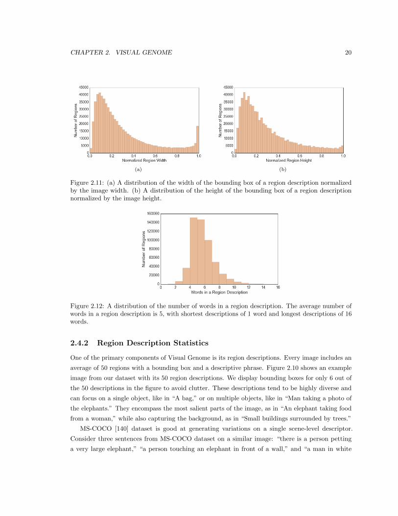
CHAPTER 2. VISUAL GENOME 20
(a) (b)
Figure 2.11: (a) A distribution of the width of the bounding box of a region description normalizedby the image width. (b) A distribution of the height of the bounding box of a region descriptionnormalized by the image height.
Figure 2.12: A distribution of the number of words in a region description. The average number ofwords in a region description is 5, with shortest descriptions of 1 word and longest descriptions of 16words.
2.4.2 Region Description Statistics
One of the primary components of Visual Genome is its region descriptions. Every image includes an
average of 50 regions with a bounding box and a descriptive phrase. Figure 2.10 shows an example
image from our dataset with its 50 region descriptions. We display bounding boxes for only 6 out of
the 50 descriptions in the figure to avoid clutter. These descriptions tend to be highly diverse and
can focus on a single object, like in “A bag,” or on multiple objects, like in “Man taking a photo of
the elephants.” They encompass the most salient parts of the image, as in “An elephant taking food
from a woman,” while also capturing the background, as in “Small buildings surrounded by trees.”
MS-COCO [140] dataset is good at generating variations on a single scene-level descriptor.
Consider three sentences from MS-COCO dataset on a similar image: “there is a person petting
a very large elephant,” “a person touching an elephant in front of a wall,” and “a man in white
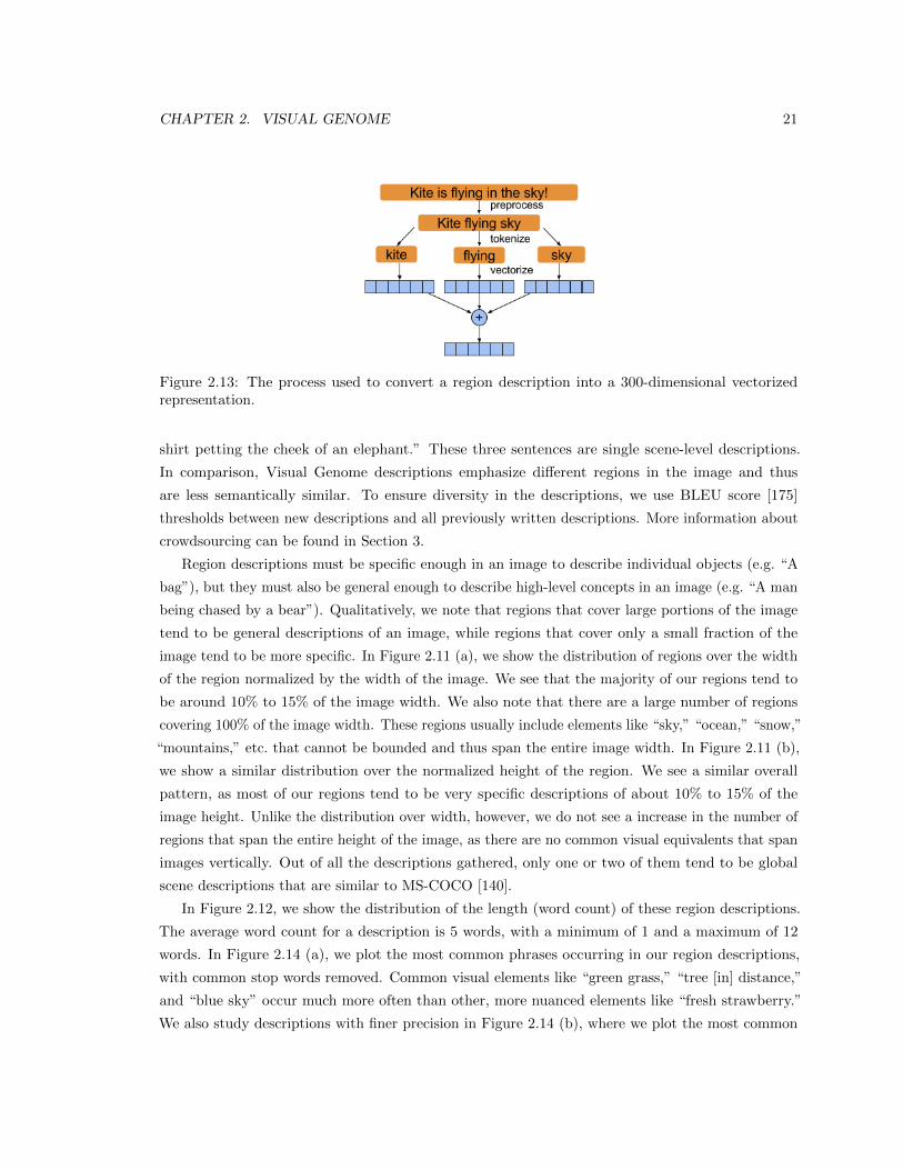
CHAPTER 2. VISUAL GENOME 21
Figure 2.13: The process used to convert a region description into a 300-dimensional vectorizedrepresentation.
shirt petting the cheek of an elephant.” These three sentences are single scene-level descriptions.
In comparison, Visual Genome descriptions emphasize different regions in the image and thus
are less semantically similar. To ensure diversity in the descriptions, we use BLEU score [175]
thresholds between new descriptions and all previously written descriptions. More information about
crowdsourcing can be found in Section 3.
Region descriptions must be specific enough in an image to describe individual objects (e.g. “A
bag”), but they must also be general enough to describe high-level concepts in an image (e.g. “A man
being chased by a bear”). Qualitatively, we note that regions that cover large portions of the image
tend to be general descriptions of an image, while regions that cover only a small fraction of the
image tend to be more specific. In Figure 2.11 (a), we show the distribution of regions over the width
of the region normalized by the width of the image. We see that the majority of our regions tend to
be around 10% to 15% of the image width. We also note that there are a large number of regions
covering 100% of the image width. These regions usually include elements like “sky,” “ocean,” “snow,”
“mountains,” etc. that cannot be bounded and thus span the entire image width. In Figure 2.11 (b),
we show a similar distribution over the normalized height of the region. We see a similar overall
pattern, as most of our regions tend to be very specific descriptions of about 10% to 15% of the
image height. Unlike the distribution over width, however, we do not see a increase in the number of
regions that span the entire height of the image, as there are no common visual equivalents that span
images vertically. Out of all the descriptions gathered, only one or two of them tend to be global
scene descriptions that are similar to MS-COCO [140].
In Figure 2.12, we show the distribution of the length (word count) of these region descriptions.
The average word count for a description is 5 words, with a minimum of 1 and a maximum of 12
words. In Figure 2.14 (a), we plot the most common phrases occurring in our region descriptions,
with common stop words removed. Common visual elements like “green grass,” “tree [in] distance,”
and “blue sky” occur much more often than other, more nuanced elements like “fresh strawberry.”
We also study descriptions with finer precision in Figure 2.14 (b), where we plot the most common
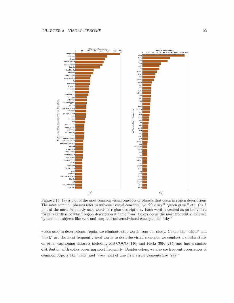
CHAPTER 2. VISUAL GENOME 22
(a) (b)
Figure 2.14: (a) A plot of the most common visual concepts or phrases that occur in region descriptions.The most common phrases refer to universal visual concepts like “blue sky,” “green grass,” etc. (b) Aplot of the most frequently used words in region descriptions. Each word is treated as an individualtoken regardless of which region description it came from. Colors occur the most frequently, followedby common objects like man and dog and universal visual concepts like “sky.”
words used in descriptions. Again, we eliminate stop words from our study. Colors like “white” and
“black” are the most frequently used words to describe visual concepts; we conduct a similar study
on other captioning datasets including MS-COCO [140] and Flickr 30K [275] and find a similar
distribution with colors occurring most frequently. Besides colors, we also see frequent occurrences of
common objects like “man” and “tree” and of universal visual elements like “sky.”
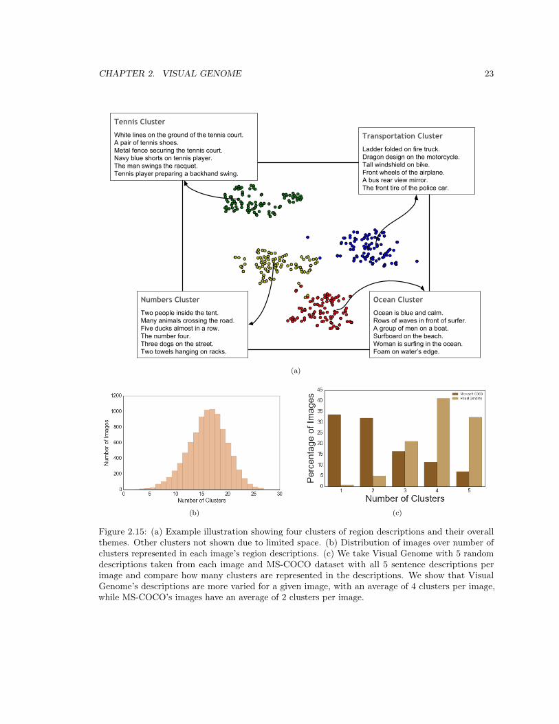
CHAPTER 2. VISUAL GENOME 23
Numbers Cluster
Two people inside the tent.Many animals crossing the road.Five ducks almost in a row.The number four.Three dogs on the street.Two towels hanging on racks.
Tennis Cluster
White lines on the ground of the tennis court.A pair of tennis shoes.Metal fence securing the tennis court.Navy blue shorts on tennis player.The man swings the racquet.Tennis player preparing a backhand swing.
Ocean Cluster
Ocean is blue and calm.Rows of waves in front of surfer.A group of men on a boat.Surfboard on the beach.Woman is surfing in the ocean.Foam on water’s edge.
Transportation Cluster
Ladder folded on fire truck.Dragon design on the motorcycle.Tall windshield on bike.Front wheels of the airplane.A bus rear view mirror.The front tire of the police car.
(a)
(b) (c)
Figure 2.15: (a) Example illustration showing four clusters of region descriptions and their overallthemes. Other clusters not shown due to limited space. (b) Distribution of images over number ofclusters represented in each image’s region descriptions. (c) We take Visual Genome with 5 randomdescriptions taken from each image and MS-COCO dataset with all 5 sentence descriptions perimage and compare how many clusters are represented in the descriptions. We show that VisualGenome’s descriptions are more varied for a given image, with an average of 4 clusters per image,while MS-COCO’s images have an average of 2 clusters per image.
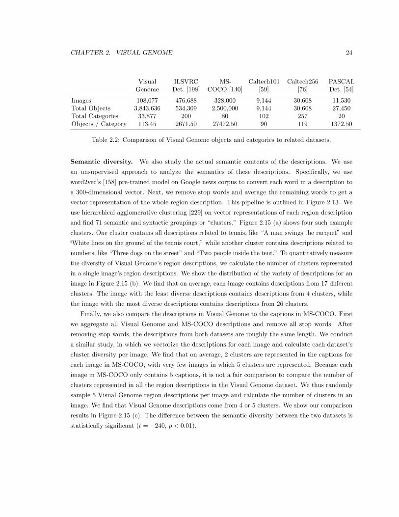
CHAPTER 2. VISUAL GENOME 24
VisualGenome
ILSVRCDet. [198]
MS-COCO [140]
Caltech101[59]
Caltech256[76]
PASCALDet. [54]
Images 108,077 476,688 328,000 9,144 30,608 11,530Total Objects 3,843,636 534,309 2,500,000 9,144 30,608 27,450Total Categories 33,877 200 80 102 257 20Objects / Category 113.45 2671.50 27472.50 90 119 1372.50
Table 2.2: Comparison of Visual Genome objects and categories to related datasets.
Semantic diversity. We also study the actual semantic contents of the descriptions. We use
an unsupervised approach to analyze the semantics of these descriptions. Specifically, we use
word2vec’s [158] pre-trained model on Google news corpus to convert each word in a description to
a 300-dimensional vector. Next, we remove stop words and average the remaining words to get a
vector representation of the whole region description. This pipeline is outlined in Figure 2.13. We
use hierarchical agglomerative clustering [229] on vector representations of each region description
and find 71 semantic and syntactic groupings or “clusters.” Figure 2.15 (a) shows four such example
clusters. One cluster contains all descriptions related to tennis, like “A man swings the racquet” and
“White lines on the ground of the tennis court,” while another cluster contains descriptions related to
numbers, like “Three dogs on the street” and “Two people inside the tent.” To quantitatively measure
the diversity of Visual Genome’s region descriptions, we calculate the number of clusters represented
in a single image’s region descriptions. We show the distribution of the variety of descriptions for an
image in Figure 2.15 (b). We find that on average, each image contains descriptions from 17 different
clusters. The image with the least diverse descriptions contains descriptions from 4 clusters, while
the image with the most diverse descriptions contains descriptions from 26 clusters.
Finally, we also compare the descriptions in Visual Genome to the captions in MS-COCO. First
we aggregate all Visual Genome and MS-COCO descriptions and remove all stop words. After
removing stop words, the descriptions from both datasets are roughly the same length. We conduct
a similar study, in which we vectorize the descriptions for each image and calculate each dataset’s
cluster diversity per image. We find that on average, 2 clusters are represented in the captions for
each image in MS-COCO, with very few images in which 5 clusters are represented. Because each
image in MS-COCO only contains 5 captions, it is not a fair comparison to compare the number of
clusters represented in all the region descriptions in the Visual Genome dataset. We thus randomly
sample 5 Visual Genome region descriptions per image and calculate the number of clusters in an
image. We find that Visual Genome descriptions come from 4 or 5 clusters. We show our comparison
results in Figure 2.15 (c). The difference between the semantic diversity between the two datasets is
statistically significant (t = −240, p < 0.01).
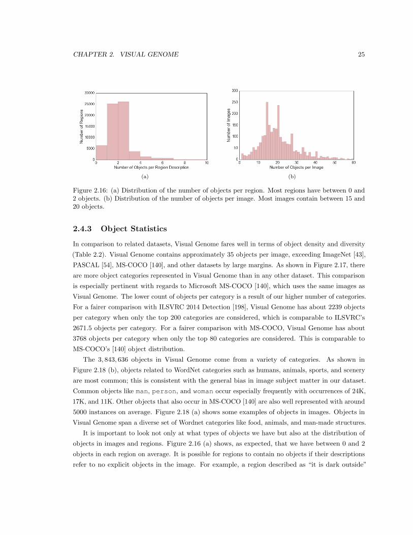
CHAPTER 2. VISUAL GENOME 25
(a) (b)
Figure 2.16: (a) Distribution of the number of objects per region. Most regions have between 0 and2 objects. (b) Distribution of the number of objects per image. Most images contain between 15 and20 objects.
2.4.3 Object Statistics
In comparison to related datasets, Visual Genome fares well in terms of object density and diversity
(Table 2.2). Visual Genome contains approximately 35 objects per image, exceeding ImageNet [43],
PASCAL [54], MS-COCO [140], and other datasets by large margins. As shown in Figure 2.17, there
are more object categories represented in Visual Genome than in any other dataset. This comparison
is especially pertinent with regards to Microsoft MS-COCO [140], which uses the same images as
Visual Genome. The lower count of objects per category is a result of our higher number of categories.
For a fairer comparison with ILSVRC 2014 Detection [198], Visual Genome has about 2239 objects
per category when only the top 200 categories are considered, which is comparable to ILSVRC’s
2671.5 objects per category. For a fairer comparison with MS-COCO, Visual Genome has about
3768 objects per category when only the top 80 categories are considered. This is comparable to
MS-COCO’s [140] object distribution.
The 3, 843, 636 objects in Visual Genome come from a variety of categories. As shown in
Figure 2.18 (b), objects related to WordNet categories such as humans, animals, sports, and scenery
are most common; this is consistent with the general bias in image subject matter in our dataset.
Common objects like man, person, and woman occur especially frequently with occurrences of 24K,
17K, and 11K. Other objects that also occur in MS-COCO [140] are also well represented with around
5000 instances on average. Figure 2.18 (a) shows some examples of objects in images. Objects in
Visual Genome span a diverse set of Wordnet categories like food, animals, and man-made structures.
It is important to look not only at what types of objects we have but also at the distribution of
objects in images and regions. Figure 2.16 (a) shows, as expected, that we have between 0 and 2
objects in each region on average. It is possible for regions to contain no objects if their descriptions
refer to no explicit objects in the image. For example, a region described as “it is dark outside”
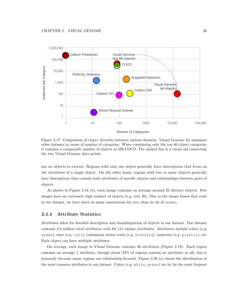
CHAPTER 2. VISUAL GENOME 26
1,000,000
100,000
10,000
1,000
100
10
1
1 10 100 1000 10,000 100,000
Number of Categories
Inst
ance
s pe
r Cat
egor
y COCO
ImageNet Detection
Visual Genome(all objects)
PASCAL Detection
Zitnick Abstract Scenes
Caltech 101Caltech 256
Caltech Pedestrian Visual Genome (top 80 objects)
Figure 2.17: Comparison of object diversity between various datasets. Visual Genome far surpassesother datasets in terms of number of categories. When considering only the top 80 object categories,it contains a comparable number of objects as MS-COCO. The dashed line is a visual aid connectingthe two Visual Genome data points.
has no objects to extract. Regions with only one object generally have descriptions that focus on
the attributes of a single object. On the other hand, regions with two or more objects generally
have descriptions that contain both attributes of specific objects and relationships between pairs of
objects.
As shown in Figure 2.16 (b), each image contains on average around 35 distinct objects. Few
images have an extremely high number of objects (e.g. over 40). Due to the image biases that exist
in the dataset, we have twice as many annotations for men than we do of women.
2.4.4 Attribute Statistics
Attributes allow for detailed description and disambiguation of objects in our dataset. Our dataset
contains 2.8 million total attributes with 68, 111 unique attributes. Attributes include colors (e.g.
green), sizes (e.g. tall), continuous action verbs (e.g. standing), materials (e.g. plastic), etc.
Each object can have multiple attributes.
On average, each image in Visual Genome contains 26 attributes (Figure 2.19). Each region
contains on average 1 attribute, though about 34% of regions contain no attribute at all; this is
primarily because many regions are relationship-focused. Figure 2.20 (a) shows the distribution of
the most common attributes in our dataset. Colors (e.g. white, green) are by far the most frequent
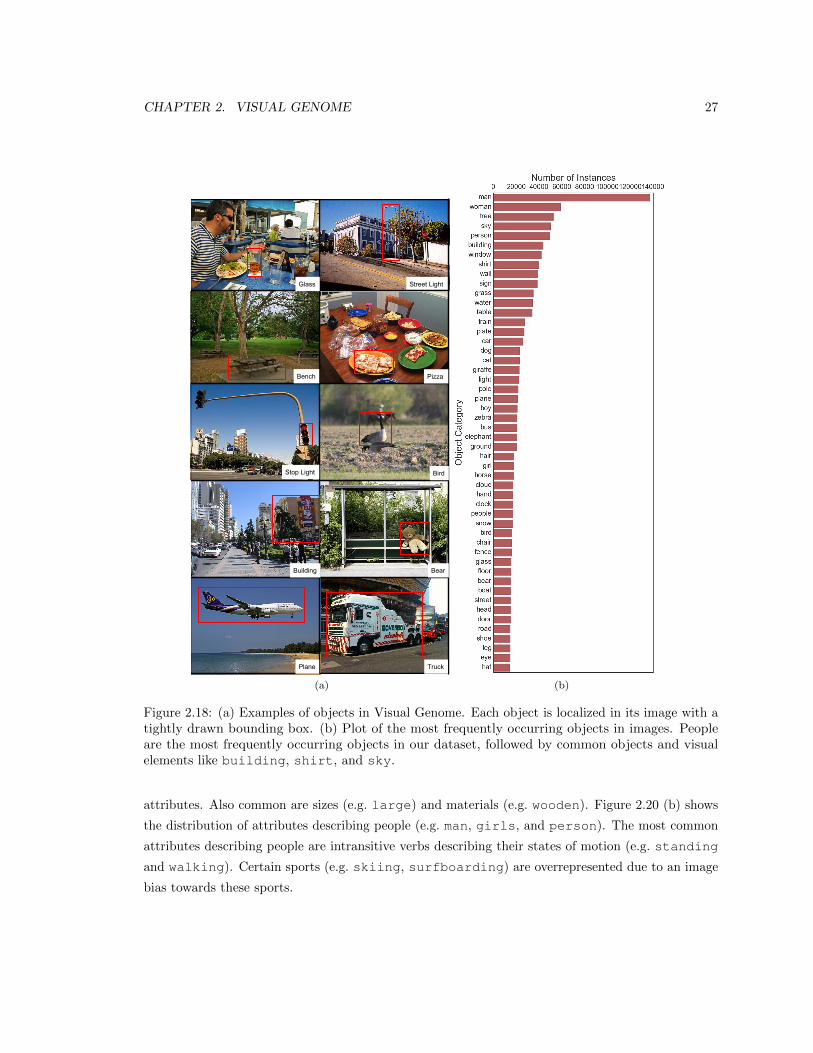
CHAPTER 2. VISUAL GENOME 27
Street LightGlass
Bench Pizza
Stop Light Bird
Building Bear
Plane Truck
(a) (b)
Figure 2.18: (a) Examples of objects in Visual Genome. Each object is localized in its image with atightly drawn bounding box. (b) Plot of the most frequently occurring objects in images. Peopleare the most frequently occurring objects in our dataset, followed by common objects and visualelements like building, shirt, and sky.
attributes. Also common are sizes (e.g. large) and materials (e.g. wooden). Figure 2.20 (b) shows
the distribution of attributes describing people (e.g. man, girls, and person). The most common
attributes describing people are intransitive verbs describing their states of motion (e.g. standing
and walking). Certain sports (e.g. skiing, surfboarding) are overrepresented due to an image
bias towards these sports.
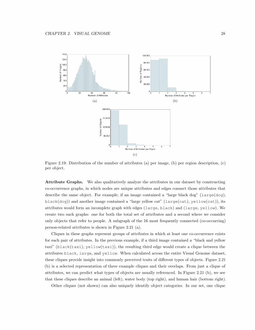
CHAPTER 2. VISUAL GENOME 28
(a) (b)
(c)
Figure 2.19: Distribution of the number of attributes (a) per image, (b) per region description, (c)per object.
Attribute Graphs. We also qualitatively analyze the attributes in our dataset by constructing
co-occurrence graphs, in which nodes are unique attributes and edges connect those attributes that
describe the same object. For example, if an image contained a “large black dog” (large(dog),
black(dog)) and another image contained a “large yellow cat” (large(cat), yellow(cat)), its
attributes would form an incomplete graph with edges (large, black) and (large, yellow). We
create two such graphs: one for both the total set of attributes and a second where we consider
only objects that refer to people. A subgraph of the 16 most frequently connected (co-occurring)
person-related attributes is shown in Figure 2.21 (a).
Cliques in these graphs represent groups of attributes in which at least one co-occurrence exists
for each pair of attributes. In the previous example, if a third image contained a “black and yellow
taxi” (black(taxi), yellow(taxi)), the resulting third edge would create a clique between the
attributes black, large, and yellow. When calculated across the entire Visual Genome dataset,
these cliques provide insight into commonly perceived traits of different types of objects. Figure 2.21
(b) is a selected representation of three example cliques and their overlaps. From just a clique of
attributes, we can predict what types of objects are usually referenced. In Figure 2.21 (b), we see
that these cliques describe an animal (left), water body (top right), and human hair (bottom right).
Other cliques (not shown) can also uniquely identify object categories. In our set, one clique
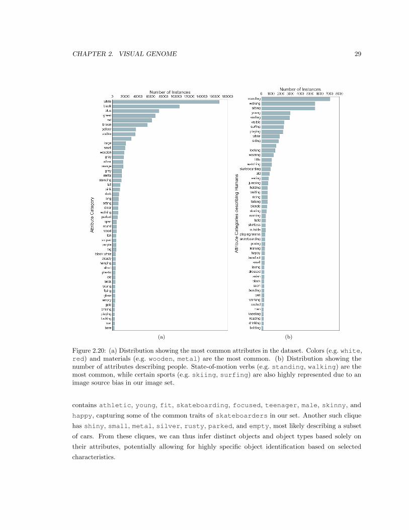
CHAPTER 2. VISUAL GENOME 29
(a) (b)
Figure 2.20: (a) Distribution showing the most common attributes in the dataset. Colors (e.g. white,red) and materials (e.g. wooden, metal) are the most common. (b) Distribution showing thenumber of attributes describing people. State-of-motion verbs (e.g. standing, walking) are themost common, while certain sports (e.g. skiing, surfing) are also highly represented due to animage source bias in our image set.
contains athletic, young, fit, skateboarding, focused, teenager, male, skinny, and
happy, capturing some of the common traits of skateboarders in our set. Another such clique
has shiny, small, metal, silver, rusty, parked, and empty, most likely describing a subset
of cars. From these cliques, we can thus infer distinct objects and object types based solely on
their attributes, potentially allowing for highly specific object identification based on selected
characteristics.
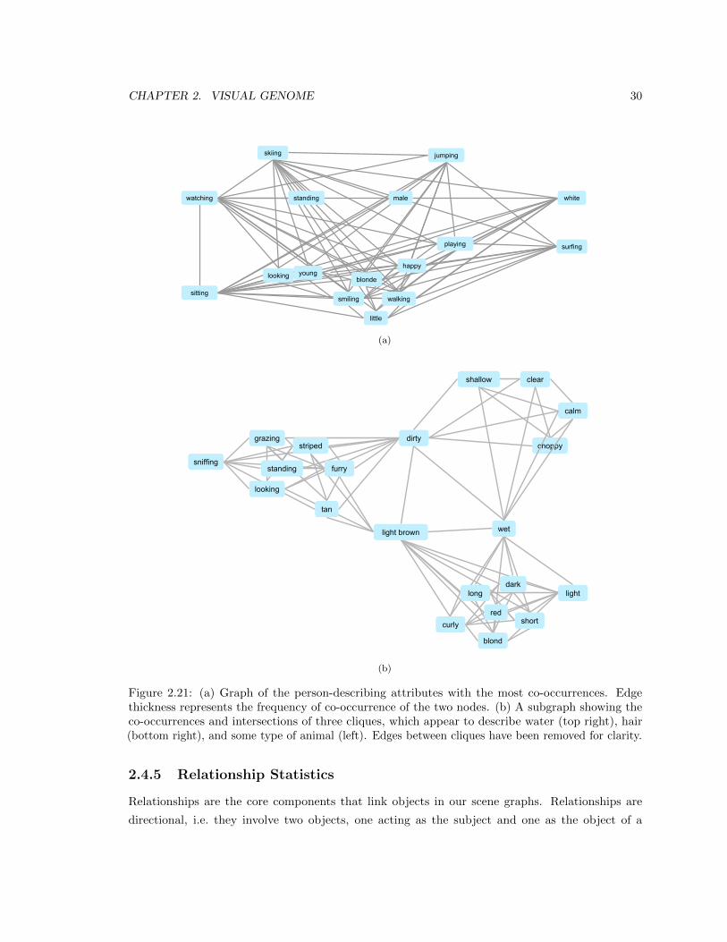
CHAPTER 2. VISUAL GENOME 30
watching
sitting
little
walkingsmiling
blonde
standing
skiing jumping
male
playing
white
surfing
happylooking young
(a)
curly
blond
shortred
longdark
light
sniffing
grazing
standing
striped
looking
furry
tan
dirty
light brown wet
shallow clear
calm
choppy
(b)
Figure 2.21: (a) Graph of the person-describing attributes with the most co-occurrences. Edgethickness represents the frequency of co-occurrence of the two nodes. (b) A subgraph showing theco-occurrences and intersections of three cliques, which appear to describe water (top right), hair(bottom right), and some type of animal (left). Edges between cliques have been removed for clarity.
2.4.5 Relationship Statistics
Relationships are the core components that link objects in our scene graphs. Relationships are
directional, i.e. they involve two objects, one acting as the subject and one as the object of a
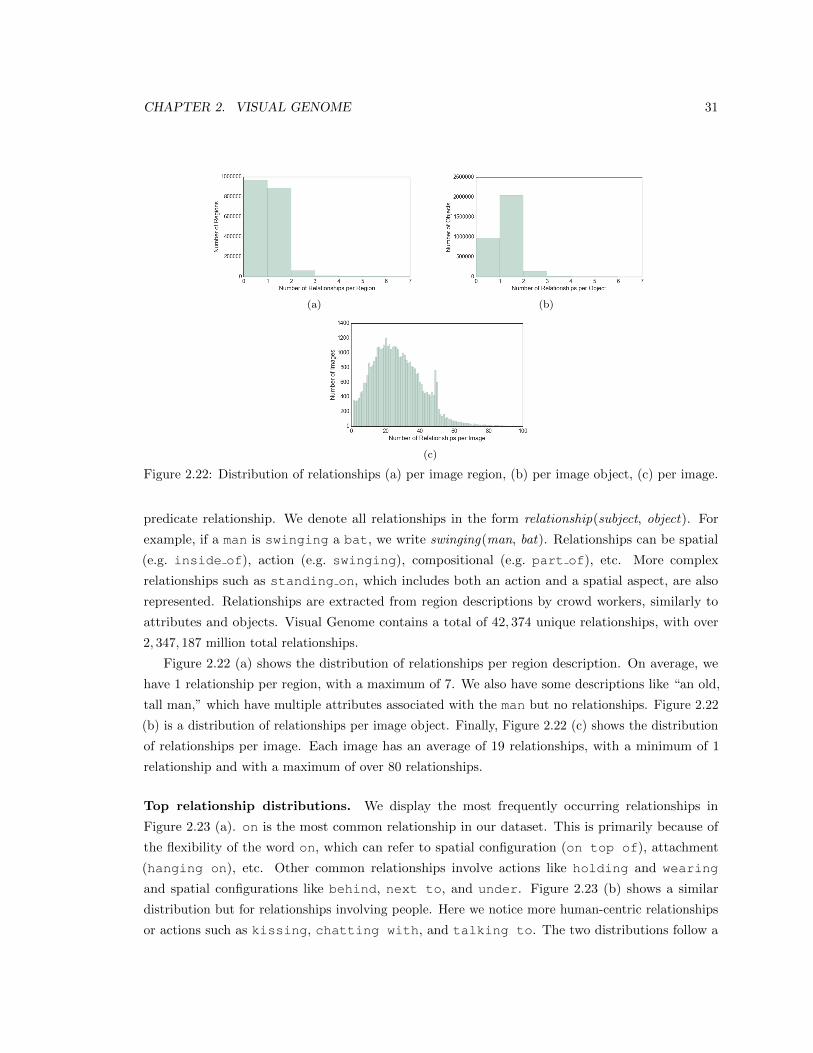
CHAPTER 2. VISUAL GENOME 31
(a) (b)
(c)
Figure 2.22: Distribution of relationships (a) per image region, (b) per image object, (c) per image.
predicate relationship. We denote all relationships in the form relationship(subject, object). For
example, if a man is swinging a bat, we write swinging(man, bat). Relationships can be spatial
(e.g. inside of), action (e.g. swinging), compositional (e.g. part of), etc. More complex
relationships such as standing on, which includes both an action and a spatial aspect, are also
represented. Relationships are extracted from region descriptions by crowd workers, similarly to
attributes and objects. Visual Genome contains a total of 42, 374 unique relationships, with over
2, 347, 187 million total relationships.
Figure 2.22 (a) shows the distribution of relationships per region description. On average, we
have 1 relationship per region, with a maximum of 7. We also have some descriptions like “an old,
tall man,” which have multiple attributes associated with the man but no relationships. Figure 2.22
(b) is a distribution of relationships per image object. Finally, Figure 2.22 (c) shows the distribution
of relationships per image. Each image has an average of 19 relationships, with a minimum of 1
relationship and with a maximum of over 80 relationships.
Top relationship distributions. We display the most frequently occurring relationships in
Figure 2.23 (a). on is the most common relationship in our dataset. This is primarily because of
the flexibility of the word on, which can refer to spatial configuration (on top of), attachment
(hanging on), etc. Other common relationships involve actions like holding and wearing
and spatial configurations like behind, next to, and under. Figure 2.23 (b) shows a similar
distribution but for relationships involving people. Here we notice more human-centric relationships
or actions such as kissing, chatting with, and talking to. The two distributions follow a
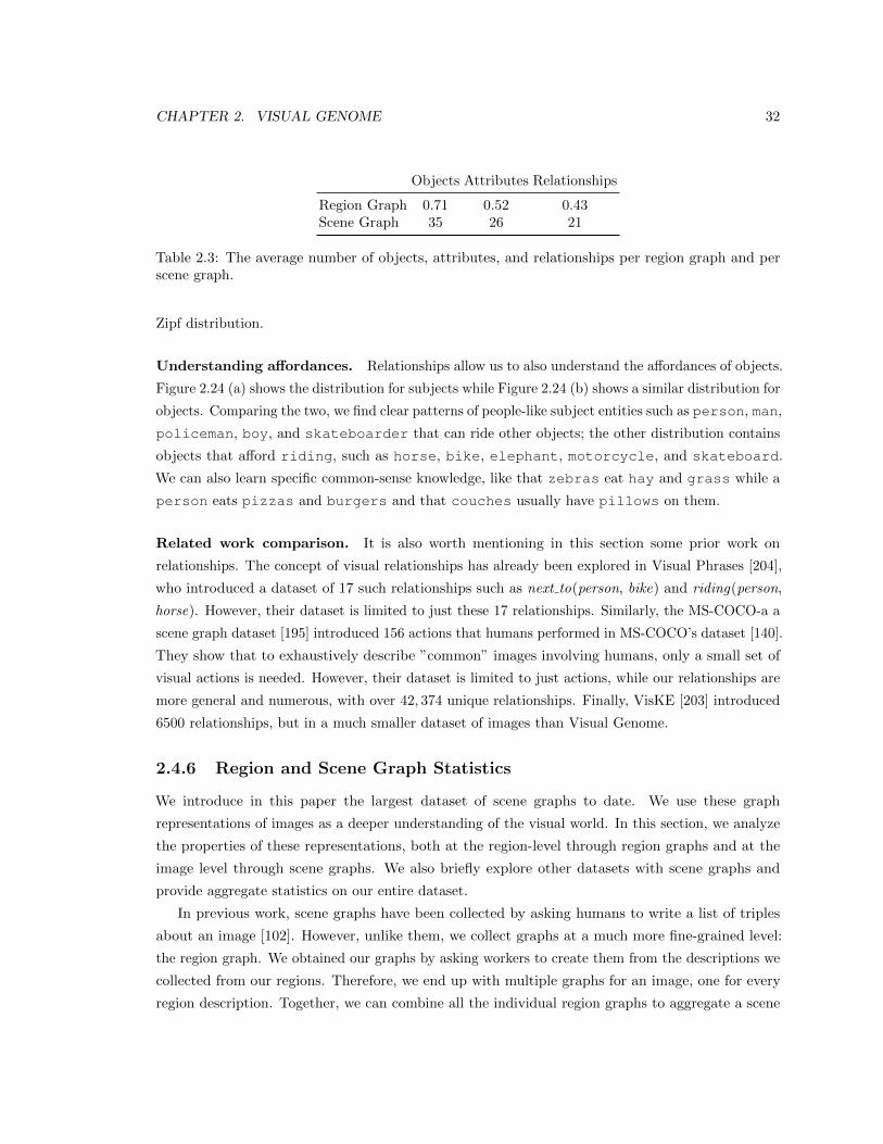
CHAPTER 2. VISUAL GENOME 32
Objects Attributes Relationships
Region Graph 0.71 0.52 0.43Scene Graph 35 26 21
Table 2.3: The average number of objects, attributes, and relationships per region graph and perscene graph.
Zipf distribution.
Understanding affordances. Relationships allow us to also understand the affordances of objects.
Figure 2.24 (a) shows the distribution for subjects while Figure 2.24 (b) shows a similar distribution for
objects. Comparing the two, we find clear patterns of people-like subject entities such as person, man,
policeman, boy, and skateboarder that can ride other objects; the other distribution contains
objects that afford riding, such as horse, bike, elephant, motorcycle, and skateboard.
We can also learn specific common-sense knowledge, like that zebras eat hay and grass while a
person eats pizzas and burgers and that couches usually have pillows on them.
Related work comparison. It is also worth mentioning in this section some prior work on
relationships. The concept of visual relationships has already been explored in Visual Phrases [204],
who introduced a dataset of 17 such relationships such as next to(person, bike) and riding(person,
horse). However, their dataset is limited to just these 17 relationships. Similarly, the MS-COCO-a a
scene graph dataset [195] introduced 156 actions that humans performed in MS-COCO’s dataset [140].
They show that to exhaustively describe ”common” images involving humans, only a small set of
visual actions is needed. However, their dataset is limited to just actions, while our relationships are
more general and numerous, with over 42, 374 unique relationships. Finally, VisKE [203] introduced
6500 relationships, but in a much smaller dataset of images than Visual Genome.
2.4.6 Region and Scene Graph Statistics
We introduce in this paper the largest dataset of scene graphs to date. We use these graph
representations of images as a deeper understanding of the visual world. In this section, we analyze
the properties of these representations, both at the region-level through region graphs and at the
image level through scene graphs. We also briefly explore other datasets with scene graphs and
provide aggregate statistics on our entire dataset.
In previous work, scene graphs have been collected by asking humans to write a list of triples
about an image [102]. However, unlike them, we collect graphs at a much more fine-grained level:
the region graph. We obtained our graphs by asking workers to create them from the descriptions we
collected from our regions. Therefore, we end up with multiple graphs for an image, one for every
region description. Together, we can combine all the individual region graphs to aggregate a scene
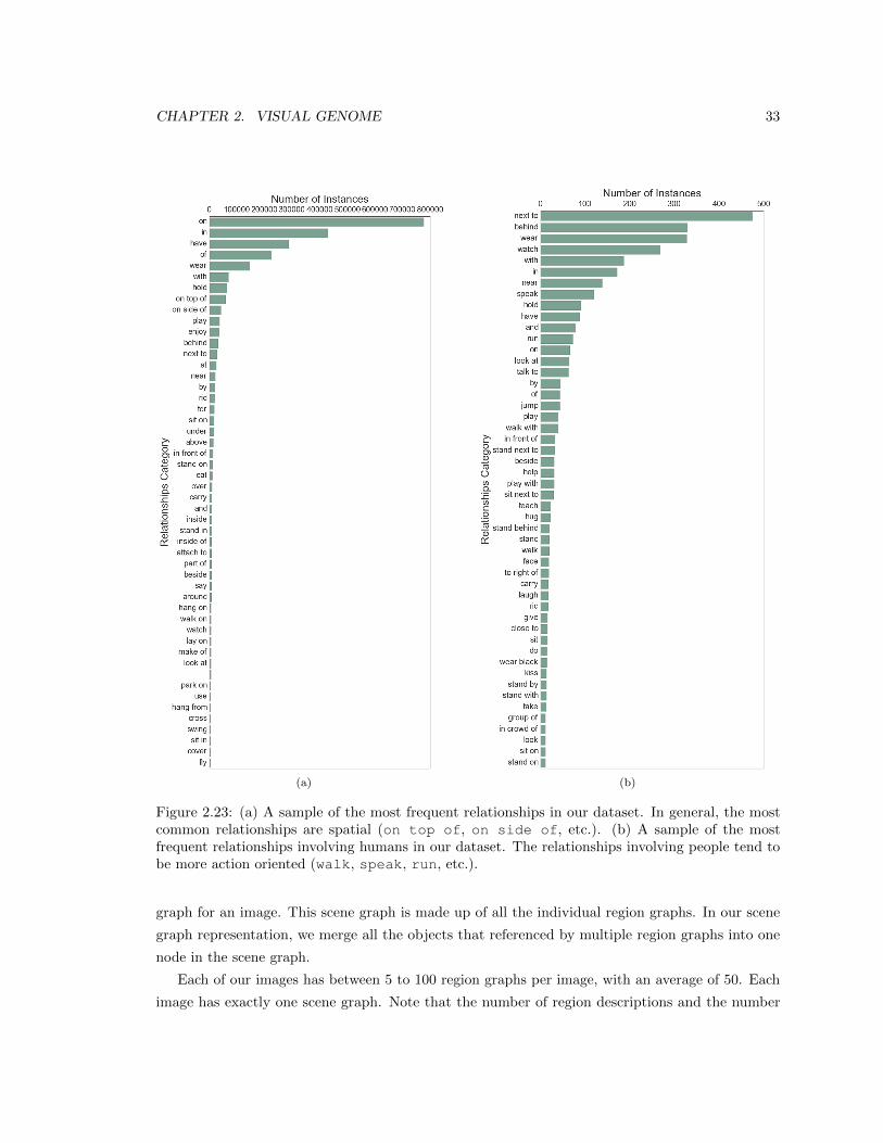
CHAPTER 2. VISUAL GENOME 33
(a) (b)
Figure 2.23: (a) A sample of the most frequent relationships in our dataset. In general, the mostcommon relationships are spatial (on top of, on side of, etc.). (b) A sample of the mostfrequent relationships involving humans in our dataset. The relationships involving people tend tobe more action oriented (walk, speak, run, etc.).
graph for an image. This scene graph is made up of all the individual region graphs. In our scene
graph representation, we merge all the objects that referenced by multiple region graphs into one
node in the scene graph.
Each of our images has between 5 to 100 region graphs per image, with an average of 50. Each
image has exactly one scene graph. Note that the number of region descriptions and the number
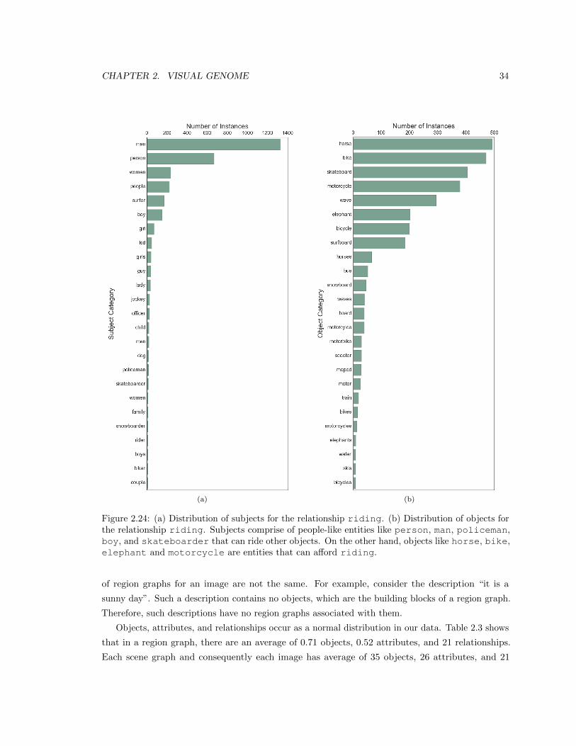
CHAPTER 2. VISUAL GENOME 34
(a) (b)
Figure 2.24: (a) Distribution of subjects for the relationship riding. (b) Distribution of objects forthe relationship riding. Subjects comprise of people-like entities like person, man, policeman,boy, and skateboarder that can ride other objects. On the other hand, objects like horse, bike,elephant and motorcycle are entities that can afford riding.
of region graphs for an image are not the same. For example, consider the description “it is a
sunny day”. Such a description contains no objects, which are the building blocks of a region graph.
Therefore, such descriptions have no region graphs associated with them.
Objects, attributes, and relationships occur as a normal distribution in our data. Table 2.3 shows
that in a region graph, there are an average of 0.71 objects, 0.52 attributes, and 21 relationships.
Each scene graph and consequently each image has average of 35 objects, 26 attributes, and 21
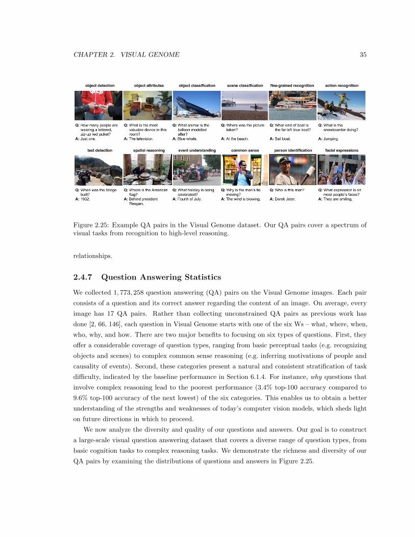
CHAPTER 2. VISUAL GENOME 35
Figure 2.25: Example QA pairs in the Visual Genome dataset. Our QA pairs cover a spectrum ofvisual tasks from recognition to high-level reasoning.
relationships.
2.4.7 Question Answering Statistics
We collected 1, 773, 258 question answering (QA) pairs on the Visual Genome images. Each pair
consists of a question and its correct answer regarding the content of an image. On average, every
image has 17 QA pairs. Rather than collecting unconstrained QA pairs as previous work has
done [2, 66, 146], each question in Visual Genome starts with one of the six Ws – what, where, when,
who, why, and how. There are two major benefits to focusing on six types of questions. First, they
offer a considerable coverage of question types, ranging from basic perceptual tasks (e.g. recognizing
objects and scenes) to complex common sense reasoning (e.g. inferring motivations of people and
causality of events). Second, these categories present a natural and consistent stratification of task
difficulty, indicated by the baseline performance in Section 6.1.4. For instance, why questions that
involve complex reasoning lead to the poorest performance (3.4% top-100 accuracy compared to
9.6% top-100 accuracy of the next lowest) of the six categories. This enables us to obtain a better
understanding of the strengths and weaknesses of today’s computer vision models, which sheds light
on future directions in which to proceed.
We now analyze the diversity and quality of our questions and answers. Our goal is to construct
a large-scale visual question answering dataset that covers a diverse range of question types, from
basic cognition tasks to complex reasoning tasks. We demonstrate the richness and diversity of our
QA pairs by examining the distributions of questions and answers in Figure 2.25.
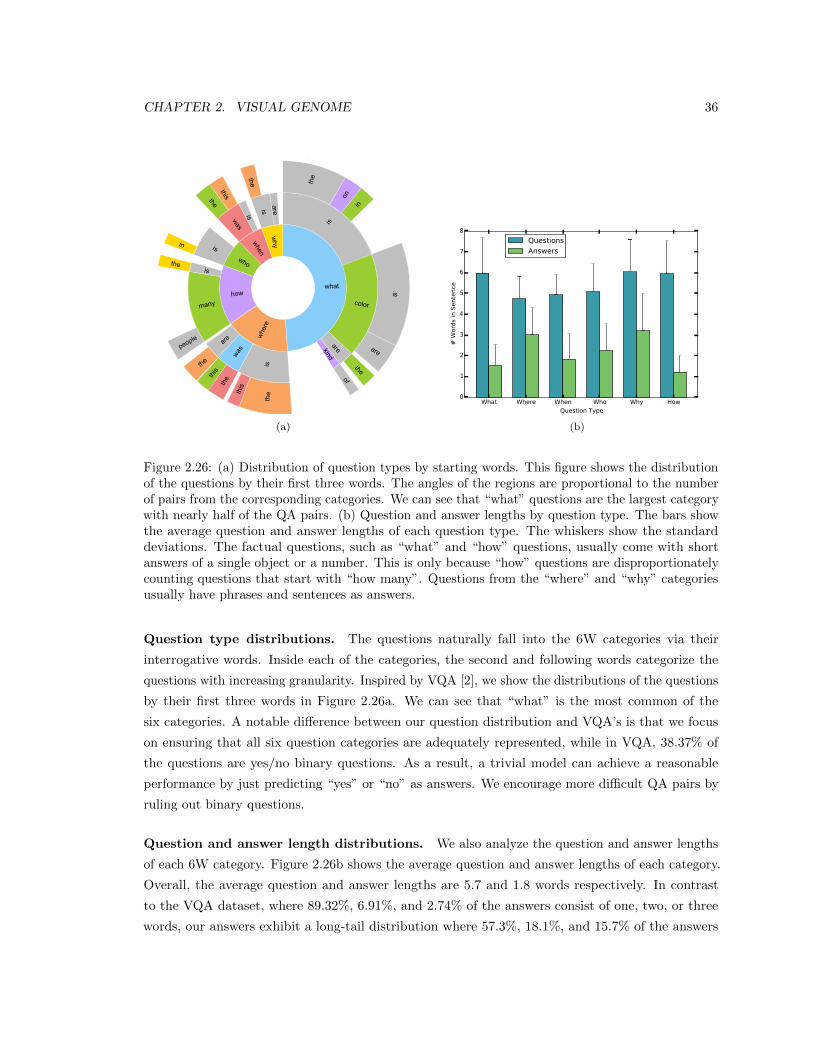
CHAPTER 2. VISUAL GENOME 36
7/9/2015 v6w_total_sunburst.svg
file://localhost/Users/yuke.zhu/Downloads/v6w_total_sunburst.svg 1/1
what
kind
of
are
the
is
in
the
on
color
are
is
who
isin when
iswas
thisthe
how
many
people
isthe
where
is
this
the
are
the
was
this
the
why
is
the
are
(a) (b)
Figure 2.26: (a) Distribution of question types by starting words. This figure shows the distributionof the questions by their first three words. The angles of the regions are proportional to the numberof pairs from the corresponding categories. We can see that “what” questions are the largest categorywith nearly half of the QA pairs. (b) Question and answer lengths by question type. The bars showthe average question and answer lengths of each question type. The whiskers show the standarddeviations. The factual questions, such as “what” and “how” questions, usually come with shortanswers of a single object or a number. This is only because “how” questions are disproportionatelycounting questions that start with “how many”. Questions from the “where” and “why” categoriesusually have phrases and sentences as answers.
Question type distributions. The questions naturally fall into the 6W categories via their
interrogative words. Inside each of the categories, the second and following words categorize the
questions with increasing granularity. Inspired by VQA [2], we show the distributions of the questions
by their first three words in Figure 2.26a. We can see that “what” is the most common of the
six categories. A notable difference between our question distribution and VQA’s is that we focus
on ensuring that all six question categories are adequately represented, while in VQA, 38.37% of
the questions are yes/no binary questions. As a result, a trivial model can achieve a reasonable
performance by just predicting “yes” or “no” as answers. We encourage more difficult QA pairs by
ruling out binary questions.
Question and answer length distributions. We also analyze the question and answer lengths
of each 6W category. Figure 2.26b shows the average question and answer lengths of each category.
Overall, the average question and answer lengths are 5.7 and 1.8 words respectively. In contrast
to the VQA dataset, where 89.32%, 6.91%, and 2.74% of the answers consist of one, two, or three
words, our answers exhibit a long-tail distribution where 57.3%, 18.1%, and 15.7% of the answers
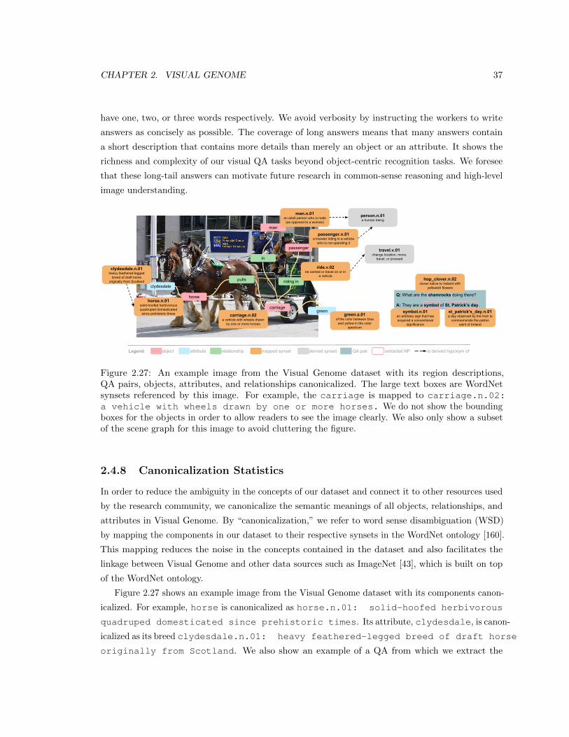
CHAPTER 2. VISUAL GENOME 37
have one, two, or three words respectively. We avoid verbosity by instructing the workers to write
answers as concisely as possible. The coverage of long answers means that many answers contain
a short description that contains more details than merely an object or an attribute. It shows the
richness and complexity of our visual QA tasks beyond object-centric recognition tasks. We foresee
that these long-tail answers can motivate future research in common-sense reasoning and high-level
image understanding.
IMG-ID: 150370
horse
clydesdalepulls
Legend: object attribute relationship
carriagegreen
carriage.n.02a vehicle with wheels drawn
by one or more horses
horse.n.01solid-hoofed herbivorous quadruped domesticated
since prehistoric times
clydesdale.n.01heavy feathered-legged
breed of draft horse originally from Scotland
man
passenger
man.n.01an adult person who is male
(as opposed to a woman)
passenger.n.01a traveler riding in a vehicle
who is not operating it
in
riding in
person.n.01a human being
mapped synset derived synset
Q: What are the shamrocks doing there?
A: They are a symbol of St. Patrick’s day.
hop_clover.n.02clover native to Ireland with
yellowish flowers
symbol.n.01an arbitrary sign that has acquired a conventional
significance
st_patrick's_day.n.01a day observed by the Irish to
commemorate the patron saint of Ireland
QA pair extracted NP is derived hyponym of
ride.v.02be carried or travel on or in
a vehicle
green.a.01of the color between blue
and yellow in the color spectrum
travel.v.01change location; move,
travel, or proceed
Figure 2.27: An example image from the Visual Genome dataset with its region descriptions,QA pairs, objects, attributes, and relationships canonicalized. The large text boxes are WordNetsynsets referenced by this image. For example, the carriage is mapped to carriage.n.02:a vehicle with wheels drawn by one or more horses. We do not show the boundingboxes for the objects in order to allow readers to see the image clearly. We also only show a subsetof the scene graph for this image to avoid cluttering the figure.
2.4.8 Canonicalization Statistics
In order to reduce the ambiguity in the concepts of our dataset and connect it to other resources used
by the research community, we canonicalize the semantic meanings of all objects, relationships, and
attributes in Visual Genome. By “canonicalization,” we refer to word sense disambiguation (WSD)
by mapping the components in our dataset to their respective synsets in the WordNet ontology [160].
This mapping reduces the noise in the concepts contained in the dataset and also facilitates the
linkage between Visual Genome and other data sources such as ImageNet [43], which is built on top
of the WordNet ontology.
Figure 2.27 shows an example image from the Visual Genome dataset with its components canon-
icalized. For example, horse is canonicalized as horse.n.01: solid-hoofed herbivorous
quadruped domesticated since prehistoric times. Its attribute, clydesdale, is canon-
icalized as its breed clydesdale.n.01: heavy feathered-legged breed of draft horse
originally from Scotland. We also show an example of a QA from which we extract the
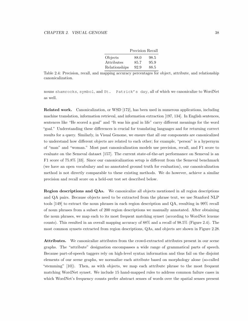
CHAPTER 2. VISUAL GENOME 38
Precision Recall
Objects 88.0 98.5Attributes 85.7 95.9Relationships 92.9 88.5
Table 2.4: Precision, recall, and mapping accuracy percentages for object, attribute, and relationshipcanonicalization.
nouns shamrocks, symbol, and St. Patrick’s day, all of which we canonicalize to WordNet
as well.
Related work. Canonicalization, or WSD [172], has been used in numerous applications, including
machine translation, information retrieval, and information extraction [197, 134]. In English sentences,
sentences like “He scored a goal” and “It was his goal in life” carry different meanings for the word
“goal.” Understanding these differences is crucial for translating languages and for returning correct
results for a query. Similarly, in Visual Genome, we ensure that all our components are canonicalized
to understand how different objects are related to each other; for example, “person” is a hypernym
of “man” and “woman.” Most past canonicalization models use precision, recall, and F1 score to
evaluate on the Semeval dataset [157]. The current state-of-the-art performance on Semeval is an
F1 score of 75.8% [33]. Since our canonicalization setup is different from the Semeval benchmark
(we have an open vocabulary and no annotated ground truth for evaluation), our canonicalization
method is not directly comparable to these existing methods. We do however, achieve a similar
precision and recall score on a held-out test set described below.
Region descriptions and QAs. We canonicalize all objects mentioned in all region descriptions
and QA pairs. Because objects need to be extracted from the phrase text, we use Stanford NLP
tools [149] to extract the noun phrases in each region description and QA, resulting in 99% recall
of noun phrases from a subset of 200 region descriptions we manually annotated. After obtaining
the noun phrases, we map each to its most frequent matching synset (according to WordNet lexeme
counts). This resulted in an overall mapping accuracy of 88% and a recall of 98.5% (Figure 2.4). The
most common synsets extracted from region descriptions, QAs, and objects are shown in Figure 2.28.
Attributes. We canonicalize attributes from the crowd-extracted attributes present in our scene
graphs. The “attribute” designation encompasses a wide range of grammatical parts of speech.
Because part-of-speech taggers rely on high-level syntax information and thus fail on the disjoint
elements of our scene graphs, we normalize each attribute based on morphology alone (so-called
“stemming” [10]). Then, as with objects, we map each attribute phrase to the most frequent
matching WordNet synset. We include 15 hand-mapped rules to address common failure cases in
which WordNet’s frequency counts prefer abstract senses of words over the spatial senses present
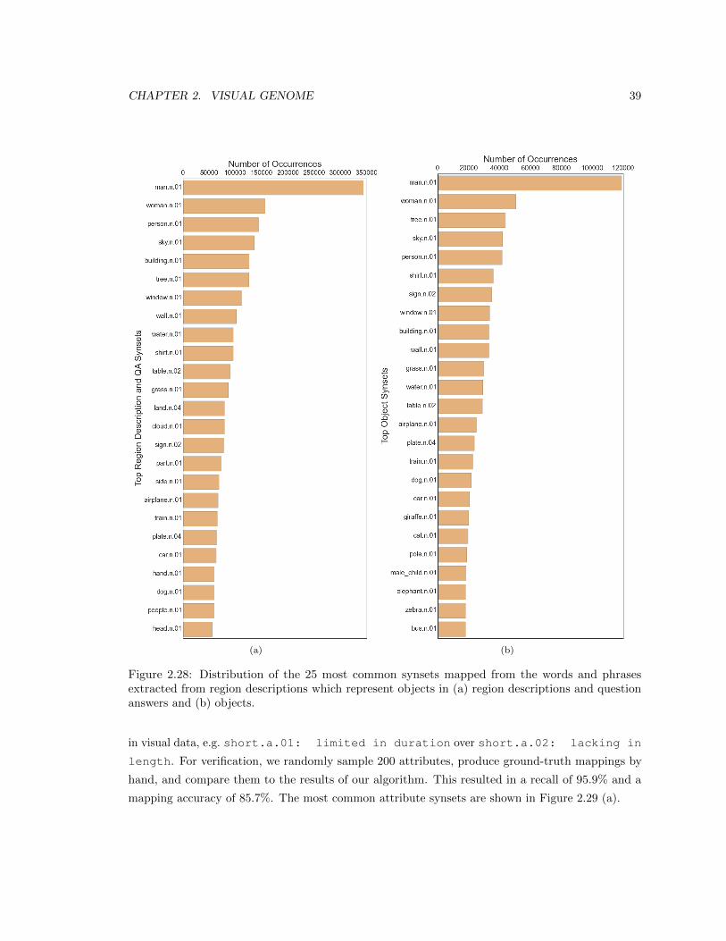
CHAPTER 2. VISUAL GENOME 39
(a) (b)
Figure 2.28: Distribution of the 25 most common synsets mapped from the words and phrasesextracted from region descriptions which represent objects in (a) region descriptions and questionanswers and (b) objects.
in visual data, e.g. short.a.01: limited in duration over short.a.02: lacking in
length. For verification, we randomly sample 200 attributes, produce ground-truth mappings by
hand, and compare them to the results of our algorithm. This resulted in a recall of 95.9% and a
mapping accuracy of 85.7%. The most common attribute synsets are shown in Figure 2.29 (a).
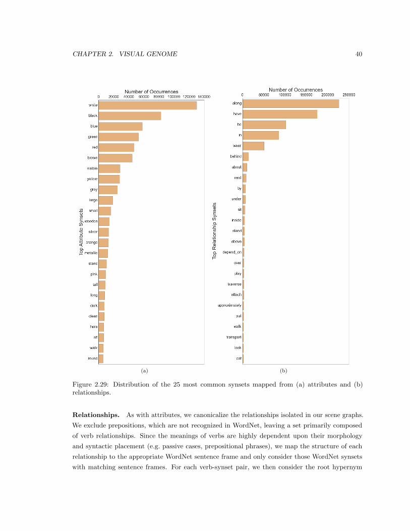
CHAPTER 2. VISUAL GENOME 40
(a) (b)
Figure 2.29: Distribution of the 25 most common synsets mapped from (a) attributes and (b)relationships.
Relationships. As with attributes, we canonicalize the relationships isolated in our scene graphs.
We exclude prepositions, which are not recognized in WordNet, leaving a set primarily composed
of verb relationships. Since the meanings of verbs are highly dependent upon their morphology
and syntactic placement (e.g. passive cases, prepositional phrases), we map the structure of each
relationship to the appropriate WordNet sentence frame and only consider those WordNet synsets
with matching sentence frames. For each verb-synset pair, we then consider the root hypernym
CHAPTER 2. VISUAL GENOME 41
of that synset to reduce potential noise from WordNet’s fine-grained sense distinctions. We also
include 20 hand-mapped rules, again to correct for WordNet’s lower representation of concrete or
spatial senses; for example, the concrete hold.v.02: have or hold in one’s hand or
grip is less frequent in WordNet than the abstract hold.v.01: cause to continue in a
certain state. For verification, we again randomly sample 200 relationships and compare the
results of our canonicalization against ground-truth mappings. This resulted in a recall of 88.5%
and a mapping accuracy of 92.9%. While several datasets, such as VerbNet [209] and FrameNet [4],
include semantic restrictions or frames to improve classification, there is no comprehensive method
of mapping to those restrictions or frames. The most common relationship synsets are shown in
Figure 2.29 (b).
Chapter 3
Crowdsourcing Strategies
Visual Genome was collected and verified entirely by crowd workers from Amazon Mechanical Turk.
In this section, we outline the pipeline employed in creating all the components of the dataset.
Each component (region descriptions, objects, attributes, relationships, region graphs, scene graphs,
questions and answers) involved multiple task stages. We mention the different strategies used to
make our data accurate and to enforce diversity in each component. We also provide background
information about the workers who helped make Visual Genome possible.
3.0.1 Crowd Workers
We used Amazon Mechanical Turk (AMT) as our primary source of annotations. Overall, a total of
over 33, 000 unique workers contributed to the dataset. The dataset was collected over the course of 6
months after 15 months of experimentation and iteration on the data representation. Approximately
800, 000 Human Intelligence Tasks (HITs) were launched on AMT, where each HIT involved creating
descriptions, questions and answers, or region graphs. Each HIT was designed such that workers
manage to earn anywhere between $6-$8 per hour if they work continuously, in line with ethical
research standards on Mechanical Turk [205]. Visual Genome HITs achieved a 94.1% retention rate,
meaning that 94.1% of workers who completed one of our tasks went ahead to do more. Table 3.1
outlines the percentage distribution of the locations of the workers. 93.02% of workers contributed
from the United States.
Figures 3.1 (a) and (b) outline the demographic distribution of our crowd workers. This data
was collected using a survey HIT. The majority of our workers were between the ages of 25 and 34
years old. Our youngest contributor was 18 years and the oldest was 68 years old. We also had a
near-balanced split of 54.15% male and 45.85% female workers.
42
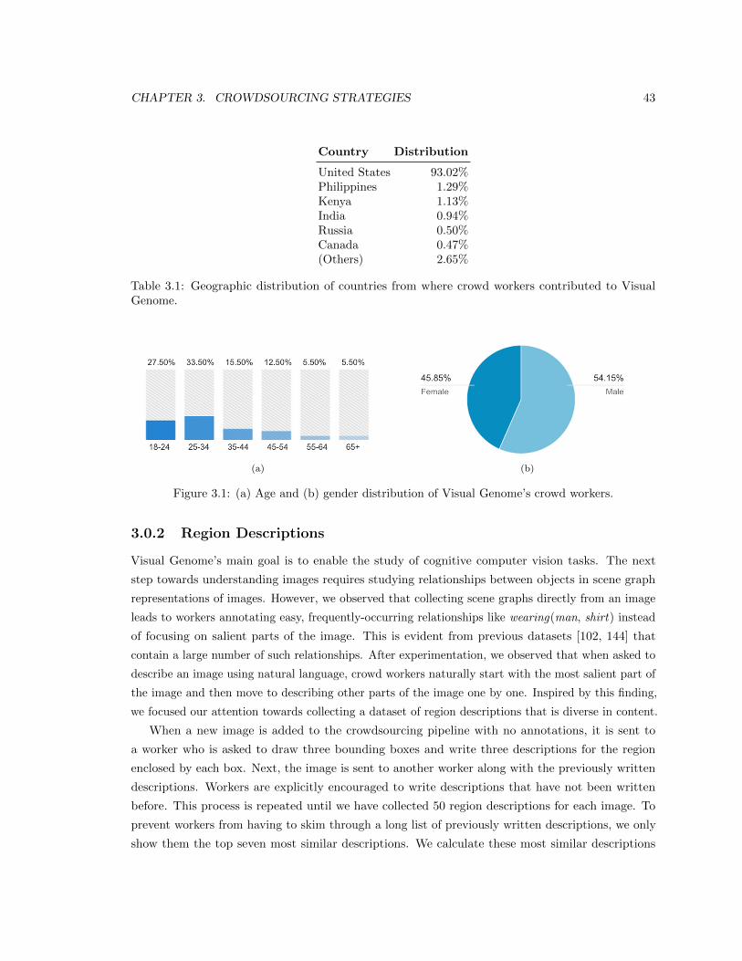
CHAPTER 3. CROWDSOURCING STRATEGIES 43
Country Distribution
United States 93.02%Philippines 1.29%Kenya 1.13%India 0.94%Russia 0.50%Canada 0.47%(Others) 2.65%
Table 3.1: Geographic distribution of countries from where crowd workers contributed to VisualGenome.
(a) (b)
Figure 3.1: (a) Age and (b) gender distribution of Visual Genome’s crowd workers.
3.0.2 Region Descriptions
Visual Genome’s main goal is to enable the study of cognitive computer vision tasks. The next
step towards understanding images requires studying relationships between objects in scene graph
representations of images. However, we observed that collecting scene graphs directly from an image
leads to workers annotating easy, frequently-occurring relationships like wearing(man, shirt) instead
of focusing on salient parts of the image. This is evident from previous datasets [102, 144] that
contain a large number of such relationships. After experimentation, we observed that when asked to
describe an image using natural language, crowd workers naturally start with the most salient part of
the image and then move to describing other parts of the image one by one. Inspired by this finding,
we focused our attention towards collecting a dataset of region descriptions that is diverse in content.
When a new image is added to the crowdsourcing pipeline with no annotations, it is sent to
a worker who is asked to draw three bounding boxes and write three descriptions for the region
enclosed by each box. Next, the image is sent to another worker along with the previously written
descriptions. Workers are explicitly encouraged to write descriptions that have not been written
before. This process is repeated until we have collected 50 region descriptions for each image. To
prevent workers from having to skim through a long list of previously written descriptions, we only
show them the top seven most similar descriptions. We calculate these most similar descriptions
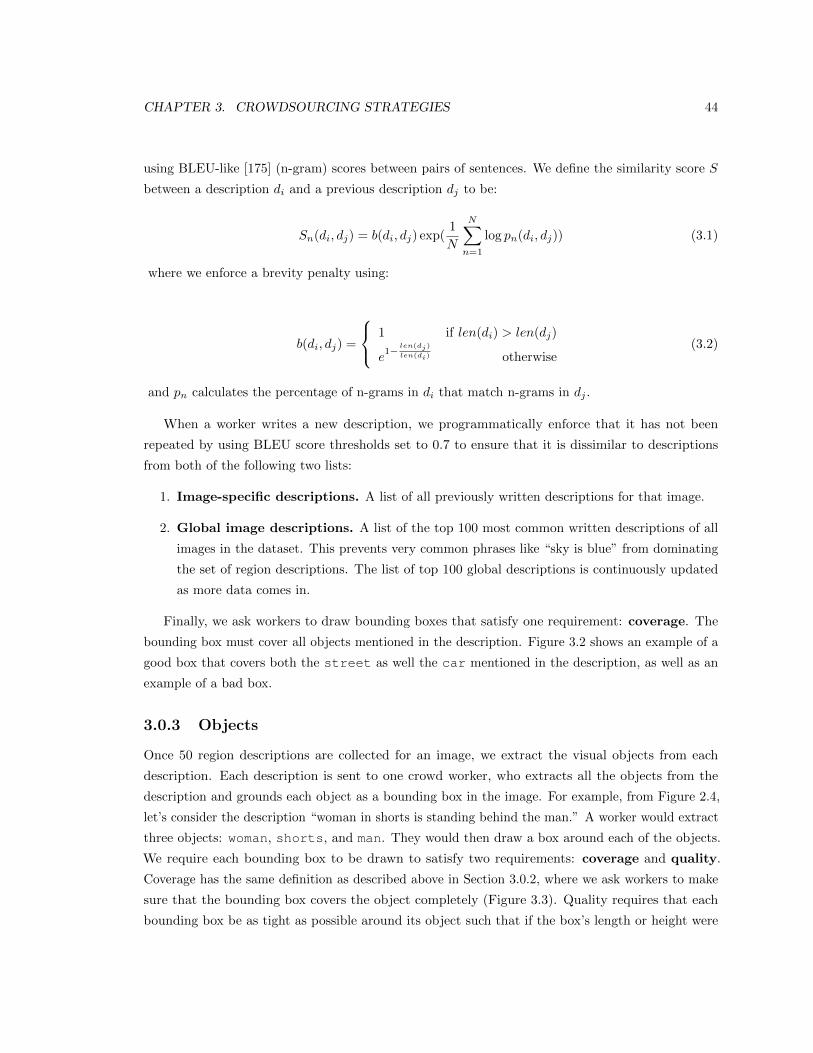
CHAPTER 3. CROWDSOURCING STRATEGIES 44
using BLEU-like [175] (n-gram) scores between pairs of sentences. We define the similarity score S
between a description di and a previous description dj to be:
Sn(di, dj) = b(di, dj) exp(1
N
N∑n=1
log pn(di, dj)) (3.1)
where we enforce a brevity penalty using:
b(di, dj) =
1 if len(di) > len(dj)
e1−
len(dj)
len(di) otherwise(3.2)
and pn calculates the percentage of n-grams in di that match n-grams in dj .
When a worker writes a new description, we programmatically enforce that it has not been
repeated by using BLEU score thresholds set to 0.7 to ensure that it is dissimilar to descriptions
from both of the following two lists:
1. Image-specific descriptions. A list of all previously written descriptions for that image.
2. Global image descriptions. A list of the top 100 most common written descriptions of all
images in the dataset. This prevents very common phrases like “sky is blue” from dominating
the set of region descriptions. The list of top 100 global descriptions is continuously updated
as more data comes in.
Finally, we ask workers to draw bounding boxes that satisfy one requirement: coverage. The
bounding box must cover all objects mentioned in the description. Figure 3.2 shows an example of a
good box that covers both the street as well the car mentioned in the description, as well as an
example of a bad box.
3.0.3 Objects
Once 50 region descriptions are collected for an image, we extract the visual objects from each
description. Each description is sent to one crowd worker, who extracts all the objects from the
description and grounds each object as a bounding box in the image. For example, from Figure 2.4,
let’s consider the description “woman in shorts is standing behind the man.” A worker would extract
three objects: woman, shorts, and man. They would then draw a box around each of the objects.
We require each bounding box to be drawn to satisfy two requirements: coverage and quality.
Coverage has the same definition as described above in Section 3.0.2, where we ask workers to make
sure that the bounding box covers the object completely (Figure 3.3). Quality requires that each
bounding box be as tight as possible around its object such that if the box’s length or height were
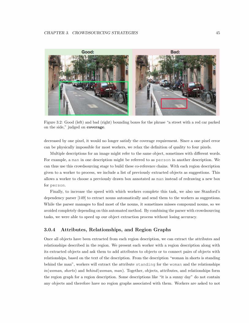
CHAPTER 3. CROWDSOURCING STRATEGIES 45
Figure 3.2: Good (left) and bad (right) bounding boxes for the phrase “a street with a red car parkedon the side,” judged on coverage.
decreased by one pixel, it would no longer satisfy the coverage requirement. Since a one pixel error
can be physically impossible for most workers, we relax the definition of quality to four pixels.
Multiple descriptions for an image might refer to the same object, sometimes with different words.
For example, a man in one description might be referred to as person in another description. We
can thus use this crowdsourcing stage to build these co-reference chains. With each region description
given to a worker to process, we include a list of previously extracted objects as suggestions. This
allows a worker to choose a previously drawn box annotated as man instead of redrawing a new box
for person.
Finally, to increase the speed with which workers complete this task, we also use Stanford’s
dependency parser [149] to extract nouns automatically and send them to the workers as suggestions.
While the parser manages to find most of the nouns, it sometimes misses compound nouns, so we
avoided completely depending on this automated method. By combining the parser with crowdsourcing
tasks, we were able to speed up our object extraction process without losing accuracy.
3.0.4 Attributes, Relationships, and Region Graphs
Once all objects have been extracted from each region description, we can extract the attributes and
relationships described in the region. We present each worker with a region description along with
its extracted objects and ask them to add attributes to objects or to connect pairs of objects with
relationships, based on the text of the description. From the description “woman in shorts is standing
behind the man”, workers will extract the attribute standing for the woman and the relationships
in(woman, shorts) and behind(woman, man). Together, objects, attributes, and relationships form
the region graph for a region description. Some descriptions like “it is a sunny day” do not contain
any objects and therefore have no region graphs associated with them. Workers are asked to not
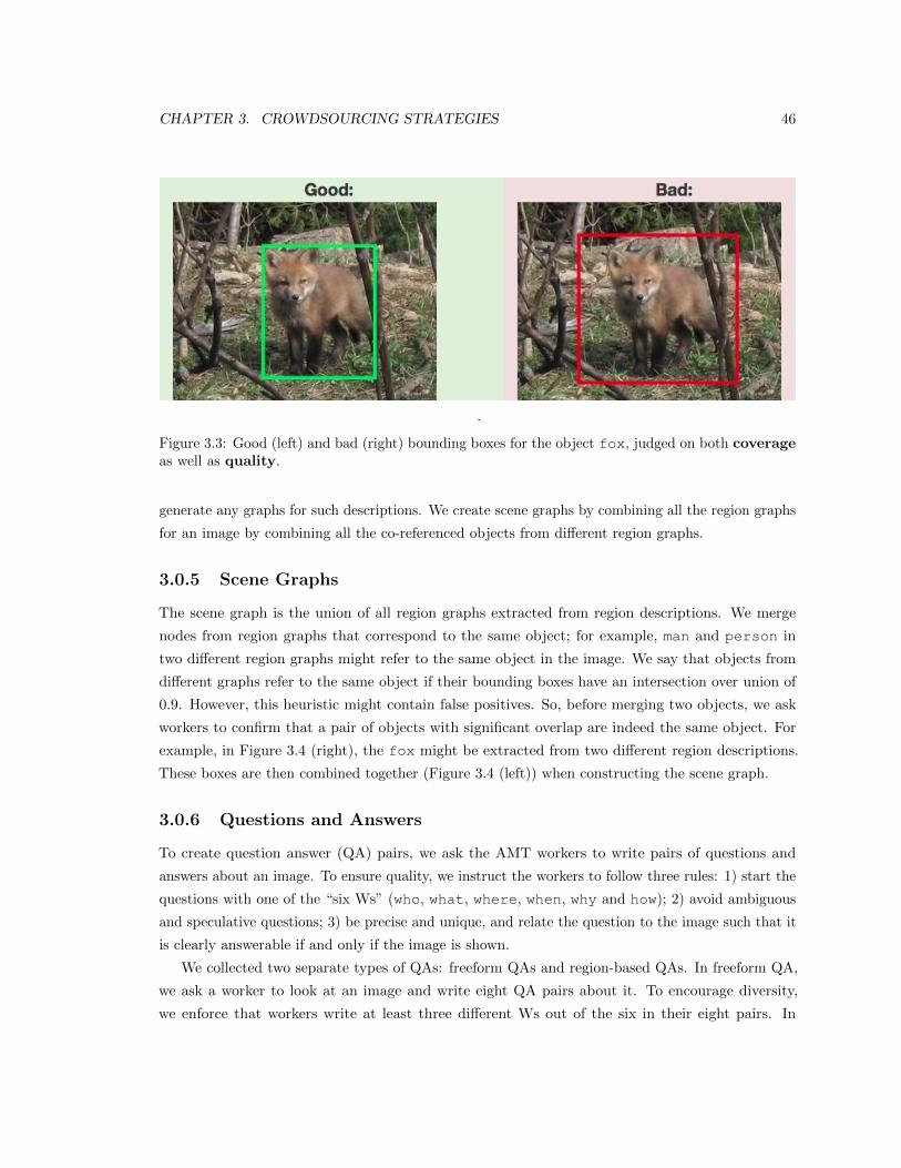
CHAPTER 3. CROWDSOURCING STRATEGIES 46
.
Figure 3.3: Good (left) and bad (right) bounding boxes for the object fox, judged on both coverageas well as quality.
generate any graphs for such descriptions. We create scene graphs by combining all the region graphs
for an image by combining all the co-referenced objects from different region graphs.
3.0.5 Scene Graphs
The scene graph is the union of all region graphs extracted from region descriptions. We merge
nodes from region graphs that correspond to the same object; for example, man and person in
two different region graphs might refer to the same object in the image. We say that objects from
different graphs refer to the same object if their bounding boxes have an intersection over union of
0.9. However, this heuristic might contain false positives. So, before merging two objects, we ask
workers to confirm that a pair of objects with significant overlap are indeed the same object. For
example, in Figure 3.4 (right), the fox might be extracted from two different region descriptions.
These boxes are then combined together (Figure 3.4 (left)) when constructing the scene graph.
3.0.6 Questions and Answers
To create question answer (QA) pairs, we ask the AMT workers to write pairs of questions and
answers about an image. To ensure quality, we instruct the workers to follow three rules: 1) start the
questions with one of the “six Ws” (who, what, where, when, why and how); 2) avoid ambiguous
and speculative questions; 3) be precise and unique, and relate the question to the image such that it
is clearly answerable if and only if the image is shown.
We collected two separate types of QAs: freeform QAs and region-based QAs. In freeform QA,
we ask a worker to look at an image and write eight QA pairs about it. To encourage diversity,
we enforce that workers write at least three different Ws out of the six in their eight pairs. In
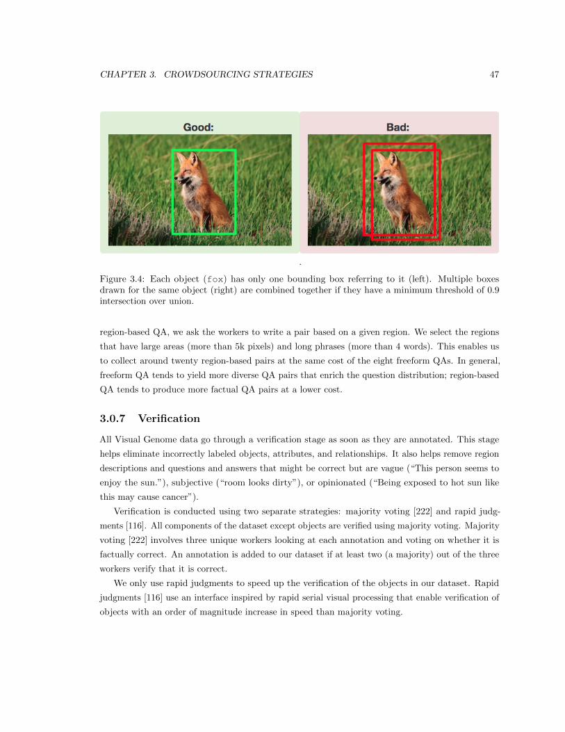
CHAPTER 3. CROWDSOURCING STRATEGIES 47
.
Figure 3.4: Each object (fox) has only one bounding box referring to it (left). Multiple boxesdrawn for the same object (right) are combined together if they have a minimum threshold of 0.9intersection over union.
region-based QA, we ask the workers to write a pair based on a given region. We select the regions
that have large areas (more than 5k pixels) and long phrases (more than 4 words). This enables us
to collect around twenty region-based pairs at the same cost of the eight freeform QAs. In general,
freeform QA tends to yield more diverse QA pairs that enrich the question distribution; region-based
QA tends to produce more factual QA pairs at a lower cost.
3.0.7 Verification
All Visual Genome data go through a verification stage as soon as they are annotated. This stage
helps eliminate incorrectly labeled objects, attributes, and relationships. It also helps remove region
descriptions and questions and answers that might be correct but are vague (“This person seems to
enjoy the sun.”), subjective (“room looks dirty”), or opinionated (“Being exposed to hot sun like
this may cause cancer”).
Verification is conducted using two separate strategies: majority voting [222] and rapid judg-
ments [116]. All components of the dataset except objects are verified using majority voting. Majority
voting [222] involves three unique workers looking at each annotation and voting on whether it is
factually correct. An annotation is added to our dataset if at least two (a majority) out of the three
workers verify that it is correct.
We only use rapid judgments to speed up the verification of the objects in our dataset. Rapid
judgments [116] use an interface inspired by rapid serial visual processing that enable verification of
objects with an order of magnitude increase in speed than majority voting.
CHAPTER 3. CROWDSOURCING STRATEGIES 48
3.0.8 Canonicalization
All the descriptions and QAs that we collect are freeform worker-generated texts. They are not
constrained by any limitations. For example, we do not force workers to refer to a man in the image as
a man. We allow them to choose to refer to the man as person, boy, man, etc. This ambiguity makes
it difficult to collect all instances of man from our dataset. In order to reduce the ambiguity in the
concepts of our dataset and connect it to other resources used by the research community, we map all
objects, attributes, relationships, and noun phrases in region descriptions and QAs to synsets in Word-
Net [160]. In the example above, person, boy, and man would map to the synsets: person.n.01
(a human being), male child.n.01 (a youthful male person) and man.n.03 (the
generic use of the word to refer to any human being) respectively. Thanks to the
WordNet hierarchy it is now possible to fuse those three expressions of the same concept into
person.n.01 (a human being), which is the lowest common ancestor node of all aforemen-
tioned synsets.
We use the Stanford NLP tools [149] to extract the noun phrases from the region descrip-
tions and QAs. Next, we map them to their most frequent matching synset in WordNet accord-
ing to WordNet lexeme counts. We then refine this simple heuristic by hand-crafting mapping
rules for the 30 most common failure cases. For example according to WordNet’s lexeme counts
the most common semantic for “table” is table.n.01 (a set of data arranged in rows
and columns). However in our data it is more likely to see pieces of furniture and therefore
bias the mapping towards table.n.02 (a piece of furniture having a smooth flat
top that is usually supported by one or more vertical legs). The objects in
our scene graphs are already noun phrases and are mapped to WordNet in the same way.
We normalize each attribute based on morphology (so called “stemming”) and map them to the
WordNet adjectives. We include 15 hand-crafted rules to address common failure cases, which typically
occur when the concrete or spatial sense of the word seen in an image is not the most common over-
all sense. For example, the synset long.a.02 (of relatively great or greater than
average spatial extension) is less common in WordNet than long.a.01 (indicating
a relatively great or greater than average duration of time), even though in-
stances of the word “long” in our images are much more likely to refer to that spatial sense.
For relationships, we ignore all prepositions as they are not recognized by WordNet. Since the
meanings of verbs are highly dependent upon their morphology and syntactic placement (e.g. passive
cases, prepositional phrases), we try to find WordNet synsets whose sentence frames match with
the context of the relationship. Sentence frames in WordNet are formalized syntactic frames in
which a certain sense of a word might appear; e.g. , play.v.01: participate in games
or sport occurs in the sentence frames “Somebody [play]s” and “Somebody [play]s something.”
For each verb-synset pair, we then consider the root hypernym of that synset to reduce potential
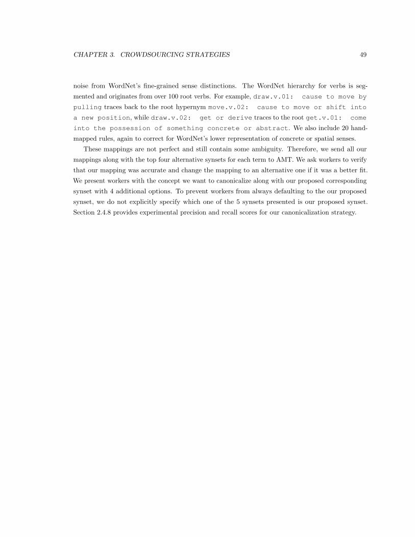
CHAPTER 3. CROWDSOURCING STRATEGIES 49
noise from WordNet’s fine-grained sense distinctions. The WordNet hierarchy for verbs is seg-
mented and originates from over 100 root verbs. For example, draw.v.01: cause to move by
pulling traces back to the root hypernym move.v.02: cause to move or shift into
a new position, while draw.v.02: get or derive traces to the root get.v.01: come
into the possession of something concrete or abstract. We also include 20 hand-
mapped rules, again to correct for WordNet’s lower representation of concrete or spatial senses.
These mappings are not perfect and still contain some ambiguity. Therefore, we send all our
mappings along with the top four alternative synsets for each term to AMT. We ask workers to verify
that our mapping was accurate and change the mapping to an alternative one if it was a better fit.
We present workers with the concept we want to canonicalize along with our proposed corresponding
synset with 4 additional options. To prevent workers from always defaulting to the our proposed
synset, we do not explicitly specify which one of the 5 synsets presented is our proposed synset.
Section 2.4.8 provides experimental precision and recall scores for our canonicalization strategy.
Chapter 4
Embracing Error to Enable Rapid
Crowdsourcing
4.1 Introduction
Social science [112, 154], interactive systems [58, 125] and machine learning [43, 140] are becoming
more and more reliant on large-scale, human-annotated data. Increasingly large annotated datasets
have unlocked a string of social scientific insights [69, 21] and machine learning performance improve-
ments [120, 71, 247]. One of the main enablers of this growth has been microtask crowdsourcing [222].
Microtask crowdsourcing marketplaces such as Amazon Mechanical Turk offer a scale and cost that
makes such annotation feasible. As a result, companies are now using crowd work to complete
hundreds of thousands of tasks per day [151].
However, even microtask crowdsourcing can be insufficiently scalable, and it remains too expensive
for use in the production of many industry-size datasets [103]. Cost is bound to the amount of work
completed per minute of effort, and existing techniques for speeding up labeling (reducing the amount
of required effort) are not scaling as quickly as the volume of data we are now producing that must
be labeled [235]. To expand the applicability of crowdsourcing, the number of items annotated per
minute of effort needs to increase substantially.
In this paper, we focus on one of the most common classes of crowdsourcing tasks [94]: binary
annotation. These tasks are yes-or-no questions, typically identifying whether or not an input has a
specific characteristic. Examples of these types of tasks are topic categorization (e.g., “Is this article
about finance?”) [207], image classification (e.g., “Is this a dog?”) [43, 140, 138], audio styles [211] and
emotion detection [138] in songs (e.g., “Is the music calm and soothing?”), word similarity (e.g., “Are
Our method for enabling rapid crowdsourcing was also a highly collaborative project, in which my main contributionswere designing the rapid interface and distributing the task to collect annotations on Amazon Mechanical Turk.
50
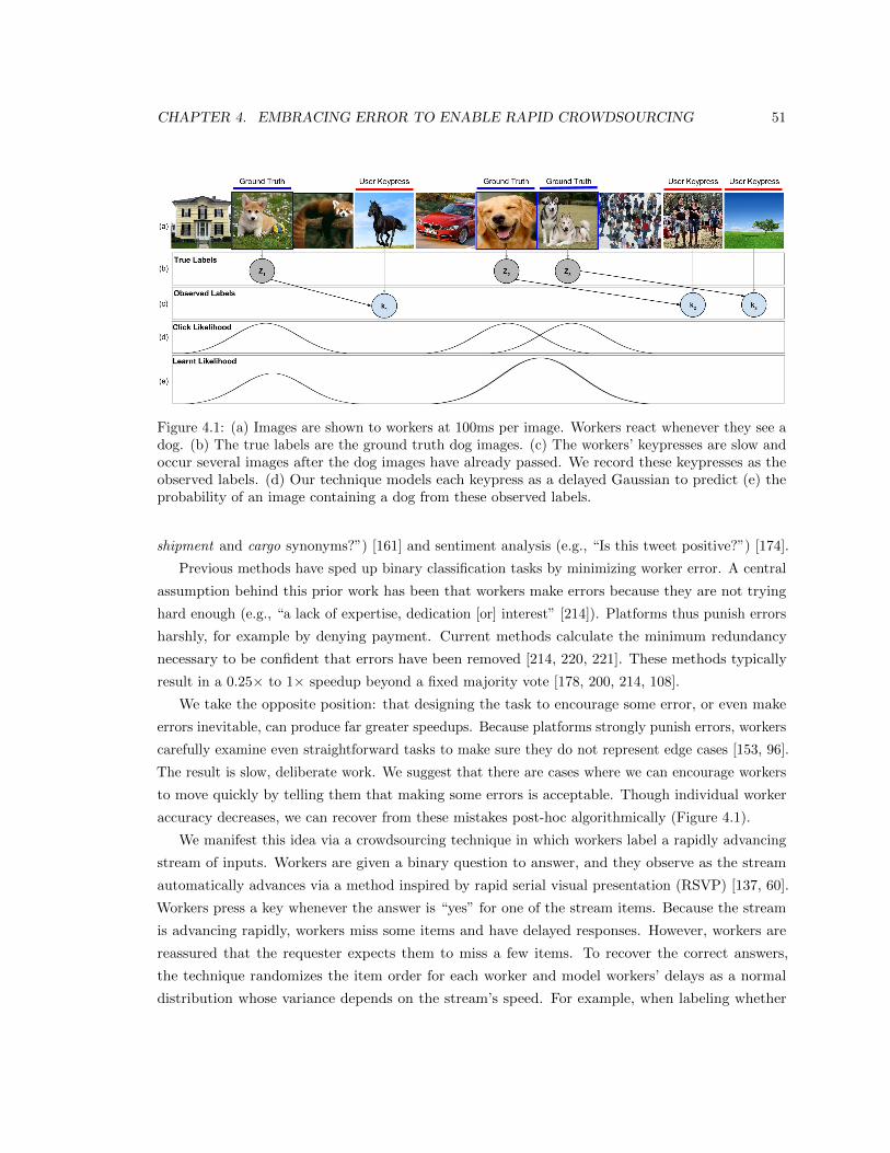
CHAPTER 4. EMBRACING ERROR TO ENABLE RAPID CROWDSOURCING 51
Figure 4.1: (a) Images are shown to workers at 100ms per image. Workers react whenever they see adog. (b) The true labels are the ground truth dog images. (c) The workers’ keypresses are slow andoccur several images after the dog images have already passed. We record these keypresses as theobserved labels. (d) Our technique models each keypress as a delayed Gaussian to predict (e) theprobability of an image containing a dog from these observed labels.
shipment and cargo synonyms?”) [161] and sentiment analysis (e.g., “Is this tweet positive?”) [174].
Previous methods have sped up binary classification tasks by minimizing worker error. A central
assumption behind this prior work has been that workers make errors because they are not trying
hard enough (e.g., “a lack of expertise, dedication [or] interest” [214]). Platforms thus punish errors
harshly, for example by denying payment. Current methods calculate the minimum redundancy
necessary to be confident that errors have been removed [214, 220, 221]. These methods typically
result in a 0.25× to 1× speedup beyond a fixed majority vote [178, 200, 214, 108].
We take the opposite position: that designing the task to encourage some error, or even make
errors inevitable, can produce far greater speedups. Because platforms strongly punish errors, workers
carefully examine even straightforward tasks to make sure they do not represent edge cases [153, 96].
The result is slow, deliberate work. We suggest that there are cases where we can encourage workers
to move quickly by telling them that making some errors is acceptable. Though individual worker
accuracy decreases, we can recover from these mistakes post-hoc algorithmically (Figure 4.1).
We manifest this idea via a crowdsourcing technique in which workers label a rapidly advancing
stream of inputs. Workers are given a binary question to answer, and they observe as the stream
automatically advances via a method inspired by rapid serial visual presentation (RSVP) [137, 60].
Workers press a key whenever the answer is “yes” for one of the stream items. Because the stream
is advancing rapidly, workers miss some items and have delayed responses. However, workers are
reassured that the requester expects them to miss a few items. To recover the correct answers,
the technique randomizes the item order for each worker and model workers’ delays as a normal
distribution whose variance depends on the stream’s speed. For example, when labeling whether
CHAPTER 4. EMBRACING ERROR TO ENABLE RAPID CROWDSOURCING 52
images have a “barking dog” in them, a self-paced worker on this task takes 1.7s per image on average.
With our technique, workers are shown a stream at 100ms per image. The technique models the
delays experienced at different input speeds and estimates the probability of intended labels from the
key presses.
We evaluate our technique by comparing the total worker time necessary to achieve the same
precision on an image labeling task as a standard setup with majority vote. The standard approach
takes three workers an average of 1.7s each for a total of 5.1s. Our technique achieves identical
precision (97%) with five workers at 100ms each, for a total of 500ms of work. The result is an order
of magnitude speedup of 10×.
This relative improvement is robust across both simple tasks, such as identifying dogs, and
complicated tasks, such as identifying “a person riding a motorcycle” (interactions between two
objects) or “people eating breakfast” (understanding relationships among many objects). We
generalize our technique to other tasks such as word similarity detection, topic classification and
sentiment analysis. Additionally, we extend our method to categorical classification tasks through a
ranked cascade of binary classifications. Finally, we test workers’ subjective mental workload and
find no measurable increase.
Contributions. We make the following contributions:
1. We introduce a rapid crowdsourcing technique that makes errors normal and even inevitable.
We show that it can be used to effectively label large datasets by achieving a speedup of an
order of magnitude on several binary labeling crowdsourcing tasks.
2. We demonstrate that our technique can be generalized to multi-label categorical labeling tasks,
combined independently with existing optimization techniques, and deployed without increasing
worker mental workload.
4.2 Related Work
The main motivation behind our work is to provide an environment where humans can make decisions
quickly. We encourage a margin of human error in the interface that is then rectified by inferring
the true labels algorithmically. In this section, we review prior work on crowdsourcing optimization
and other methods for motivating contributions. Much of this work relies on artificial intelligence
techniques: we complement this literature by changing the crowdsourcing interface rather than
focusing on the underlying statistical model.
Our technique is inspired by rapid serial visual presentation (RSVP), a technique for consuming
media rapidly by aligning it within the foveal region and advancing between items quickly [137, 60].
RSVP has already been proven to be effective at speeding up reading rates [258]. RSVP users
can react to a single target image in a sequence of images even at 125ms per image with 75%
accuracy [182]. However, when trying to recognize concepts in images, RSVP only achieves an
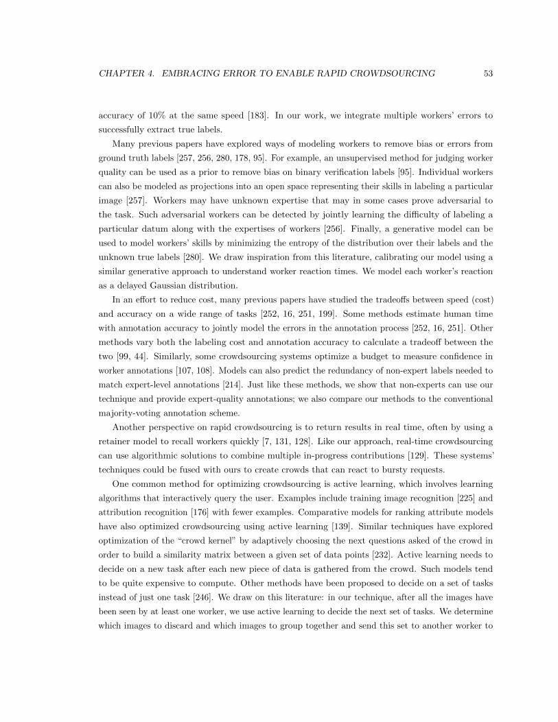
CHAPTER 4. EMBRACING ERROR TO ENABLE RAPID CROWDSOURCING 53
accuracy of 10% at the same speed [183]. In our work, we integrate multiple workers’ errors to
successfully extract true labels.
Many previous papers have explored ways of modeling workers to remove bias or errors from
ground truth labels [257, 256, 280, 178, 95]. For example, an unsupervised method for judging worker
quality can be used as a prior to remove bias on binary verification labels [95]. Individual workers
can also be modeled as projections into an open space representing their skills in labeling a particular
image [257]. Workers may have unknown expertise that may in some cases prove adversarial to
the task. Such adversarial workers can be detected by jointly learning the difficulty of labeling a
particular datum along with the expertises of workers [256]. Finally, a generative model can be
used to model workers’ skills by minimizing the entropy of the distribution over their labels and the
unknown true labels [280]. We draw inspiration from this literature, calibrating our model using a
similar generative approach to understand worker reaction times. We model each worker’s reaction
as a delayed Gaussian distribution.
In an effort to reduce cost, many previous papers have studied the tradeoffs between speed (cost)
and accuracy on a wide range of tasks [252, 16, 251, 199]. Some methods estimate human time
with annotation accuracy to jointly model the errors in the annotation process [252, 16, 251]. Other
methods vary both the labeling cost and annotation accuracy to calculate a tradeoff between the
two [99, 44]. Similarly, some crowdsourcing systems optimize a budget to measure confidence in
worker annotations [107, 108]. Models can also predict the redundancy of non-expert labels needed to
match expert-level annotations [214]. Just like these methods, we show that non-experts can use our
technique and provide expert-quality annotations; we also compare our methods to the conventional
majority-voting annotation scheme.
Another perspective on rapid crowdsourcing is to return results in real time, often by using a
retainer model to recall workers quickly [7, 131, 128]. Like our approach, real-time crowdsourcing
can use algorithmic solutions to combine multiple in-progress contributions [129]. These systems’
techniques could be fused with ours to create crowds that can react to bursty requests.
One common method for optimizing crowdsourcing is active learning, which involves learning
algorithms that interactively query the user. Examples include training image recognition [225] and
attribution recognition [176] with fewer examples. Comparative models for ranking attribute models
have also optimized crowdsourcing using active learning [139]. Similar techniques have explored
optimization of the “crowd kernel” by adaptively choosing the next questions asked of the crowd in
order to build a similarity matrix between a given set of data points [232]. Active learning needs to
decide on a new task after each new piece of data is gathered from the crowd. Such models tend
to be quite expensive to compute. Other methods have been proposed to decide on a set of tasks
instead of just one task [246]. We draw on this literature: in our technique, after all the images have
been seen by at least one worker, we use active learning to decide the next set of tasks. We determine
which images to discard and which images to group together and send this set to another worker to
CHAPTER 4. EMBRACING ERROR TO ENABLE RAPID CROWDSOURCING 54
Figure 4.2: (a) Task instructions inform workers that we expect them to make mistakes since theitems will be displayed rapidly. (b) A string of countdown images prepares them for the rate at whichitems will be displayed. (c) An example image of a “dog” shown in the stream—the two imagesappearing behind it are included for clarity but are not displayed to workers. (d) When the workerpresses a key, we show the last four images below the stream of images to indicate which imagesmight have just been labeled.
gather more information.
Finally, there is a group of techniques that attempt to optimize label collection by reducing
the number of questions that must be answered by the crowd. For example, a hierarchy in label
distribution can reduce the annotation search space [44], and information gain can reduce the number
of labels necessary to build large taxonomies using a crowd [35, 14]. Methods have also been proposed
to maximize accuracy of object localization in images [230] and videos [249]. Previous labels can also
be used as a prior to optimize acquisition of new types of annotations [15]. One of the benefits of
our technique is that it can be used independently of these others to jointly improve crowdsourcing
schemes. We demonstrate the gains of such a combination in our evaluation.
4.3 Error-Embracing Crowdsourcing
Current microtask crowdsourcing platforms like Amazon Mechanical Turk incentivize workers to
avoid rejections [96, 153], resulting in slow and meticulous work. But is such careful work necessary
to build an accurate dataset? In this section, we detail our technique for rapid crowdsourcing by
encouraging less accurate work.
The design space of such techniques must consider which tradeoffs are acceptable to make. The
first relevant dimension is accuracy. When labeling a large dataset (e.g., building a dataset of ten
thousand articles about housing), precision is often the highest priority: articles labeled as on-topic
by the system must in fact be about housing. Recall, on the other hand, is often less important,
because there is typically a large amount of available unlabeled data: even if the system misses some
on-topic articles, the system can label more items until it reaches the desired dataset size. We thus
develop an approach for producing high precision at high speed, sacrificing some recall if necessary.
CHAPTER 4. EMBRACING ERROR TO ENABLE RAPID CROWDSOURCING 55
The second design dimension involves the task characteristics. Many large-scale crowdsourcing
tasks involve closed-ended responses such as binary or categorical classifications. These tasks have
two useful properties. First, they are time-bound by users’ perception and cognition speed rather
than motor (e.g., pointing, typing) speed [34], since acting requires only a single button press. Second,
it is possible to aggregate responses automatically, for example with majority vote. Open-ended
crowdsourcing tasks such as writing [8] or transcription are often time-bound by data entry motor
speeds and cannot be automatically aggregated. Thus, with our technique, we focus on closed-ended
tasks.
4.3.1 Rapid crowdsourcing of binary decision tasks
Binary questions are one of the most common classes of crowdsourcing tasks. Each yes-or-no question
gathers a label on whether each item has a certain characteristic. In our technique, rather than
letting workers focus on each item too carefully, we display each item for a specific period of time
before moving on to the next one in a rapid slideshow. For example, in the context of an image
verification task, we show workers a stream of images and ask them to press the spacebar whenever
they see a specific class of image. In the example in Figure 4.2, we ask them to react whenever they
see a “dog.”
The main parameter in this approach is the length of time each item is visible. To determine
the best option, we begin by allowing workers to work at their own pace. This establishes an initial
average time period, which we then slowly decrease in successive versions until workers start making
mistakes [34]. Once we have identified this error point, we can algorithmically model workers’ latency
and errors to extract the true labels.
To avoid stressing out workers, it is important that the task instructions convey the nature of
the rapid task and the fact that we expect them to make some errors. Workers are first shown a set
of instructions (Figure 4.2(a)) for the task. They are warned that reacting to every single correct
image on time is not feasible and thus not expected. We also warn them that we have placed a small
number of items in the set that we know to be positive items. These help us calibrate each worker’s
speed and also provide us with a mechanism to reject workers who do not react to any of the items.
Once workers start the stream (Figure 4.2(b)), it is important to prepare them for pace of the
task. We thus show a film-style countdown for the first few seconds that decrements to zero at
the same interval as the main task. Without these countdown images, workers use up the first few
seconds getting used to the pace and speed. Figure 4.2(c) shows an example “dog” image that is
displayed in front of the user. The dimensions of all items (images) shown are held constant to avoid
having to adjust to larger or smaller visual ranges.
When items are displayed for less than 400ms, workers tend to react to all positive items with a
delay. If the interface only reacts with a simple confirmation when workers press the spacebar, many
workers worry that they are too late because another item is already on the screen. Our solution is

CHAPTER 4. EMBRACING ERROR TO ENABLE RAPID CROWDSOURCING 56
Figure 4.3: Example raw worker outputs from our interface. Each image was displayed for 100msand workers were asked to react whenever they saw images of “a person riding a motorcycle.” Imagesare shown in the same order they appeared in for the worker. Positive images are shown with a bluebar below them and users’ keypresses are shown as red bars below the image to which they reacted.
to also briefly display the last four items previously shown when the spacebar is pressed, so that
workers see the one they intended and also gather an intuition for how far back the model looks.
For example, in Figure 4.2(d), we show a worker pressing the spacebar on an image of a horse. We
anticipate that the worker was probably delayed, and we display the last four items to acknowledge
that we have recorded the keypress. We ask all workers to first complete a qualification task in which
they receive feedback on how quickly we expect them to react. They pass the qualification task only
if they achieve a recall of 0.6 and precision of 0.9 on a stream of 200 items with 25 positives. We
measure precision as the fraction of worker reactions that were within 500ms of a positive cue.
In Figure 4.3, we show two sample outputs from our interface. Workers were shown images for
100ms each. They were asked to press the spacebar whenever they saw an image of “a person riding
a motorcycle.” The images with blue bars underneath them are ground truth images of “a person
riding a motorcycle.” The images with red bars show where workers reacted. The important element
is that red labels are often delayed behind blue ground truth and occasionally missed entirely. Both
Figures 4.3(a) and 4.3(b) have 100 images each with 5 correct images.
Because of workers’ reaction delay, the data from one worker has considerable uncertainty. We
thus show the same set of items to multiple workers in different random orders and collect independent
sets of keypresses. This randomization will produce a cleaner signal in aggregate and later allow us
to estimate the images to which each worker intended to react.
Given the speed of the images, workers are not able to detect every single positive image. For
example, the last positive image in Figure 4.3(a) and the first positive image in Figure 4.3(b) are not
detected. Previous work on RSVP found a phenomenon called “attention blink” [18], in which a
CHAPTER 4. EMBRACING ERROR TO ENABLE RAPID CROWDSOURCING 57
worker is momentarily blind to successive positive images. However, we find that even if two images
of “a person riding a motorcycle” occur consecutively, workers are able to detect both and react twice
(Figures 4.3(a) and 4.3(b)). If workers are forced to react in intervals of less than 400ms, though, the
signal we extract is too noisy for our model to estimate the positive items.
4.3.2 Multi-Class Classification for Categorical Data
So far, we have described how rapid crowdsourcing can be used for binary verification tasks. Now
we extend it to handle multi-class classification. Theoretically, all multi-class classification can be
broken down into a series of binary verifications. For example, if there are N classes, we can ask N
binary questions of whether an item is in each class. Given a list of items, we use our technique to
classify them one class at a time. After every iteration, we remove all the positively classified items
for a particular class. We use the rest of the items to detect the next class.
Assuming all the classes contain an equal number of items, the order in which we detect classes
should not matter. A simple baseline approach would choose a class at random and attempt to detect
all items for that class first. However, if the distribution of items is not equal among classes, this
method would be inefficient. Consider the case where we are trying to classify items into 10 classes,
and one class has 1000 items while all other classes have 10 items. In the worst case, if we classify
the class with 1000 examples last, those 1000 images would go through our interface 10 times (once
for every class). Instead, if we had detected the large class first, we would be able to classify those
1000 images and they would only go through our interface once. With this intuition, we propose
a class-optimized approach that classifies the most common class of items first. We maximize the
number of items we classify at every iteration, reducing the total number of binary verifications
required.
4.4 Model
To translate workers’ delayed and potentially erroneous actions into identifications of the positive
items, we need to model their behavior. We do this by calculating the probability that a particular
item is in the positive class given that the user reacted a given period after the item was displayed.
By combining these probabilities across several workers with different random orders of the same
images, these probabilities sum up to identify the correct items.
We use maximum likelihood estimation to predict the probability of an item being a positive
example. Given a set of items I = {I1, . . . , In}, we send them to W workers in a different random
order for each. From each worker w, we collect a set of keypresses Cw = {cw1 , . . . , cwk } where w ∈Wand k is the total number of keypresses from w. Our aim is to calculate the probability of a given
item P (Ii) being a positive example. Given that we collect keypresses from W workers:
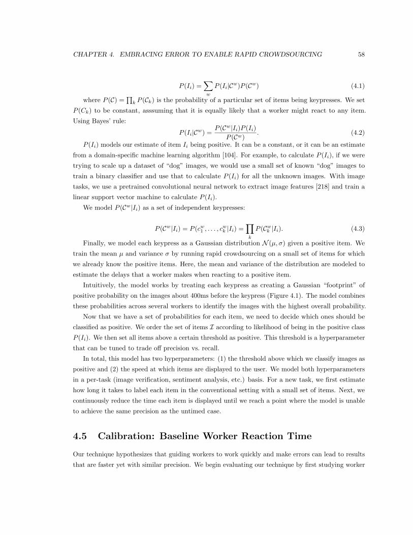
CHAPTER 4. EMBRACING ERROR TO ENABLE RAPID CROWDSOURCING 58
P (Ii) =∑w
P (Ii|Cw)P (Cw) (4.1)
where P (C) =∏k P (Ck) is the probability of a particular set of items being keypresses. We set
P (Ck) to be constant, asssuming that it is equally likely that a worker might react to any item.
Using Bayes’ rule:
P (Ii|Cw) =P (Cw|Ii)P (Ii)
P (Cw). (4.2)
P (Ii) models our estimate of item Ii being positive. It can be a constant, or it can be an estimate
from a domain-specific machine learning algorithm [104]. For example, to calculate P (Ii), if we were
trying to scale up a dataset of “dog” images, we would use a small set of known “dog” images to
train a binary classifier and use that to calculate P (Ii) for all the unknown images. With image
tasks, we use a pretrained convolutional neural network to extract image features [218] and train a
linear support vector machine to calculate P (Ii).
We model P (Cw|Ii) as a set of independent keypresses:
P (Cw|Ii) = P (cw1 , . . . , cwk |Ii) =
∏k
P (Cwk |Ii). (4.3)
Finally, we model each keypress as a Gaussian distribution N (µ, σ) given a positive item. We
train the mean µ and variance σ by running rapid crowdsourcing on a small set of items for which
we already know the positive items. Here, the mean and variance of the distribution are modeled to
estimate the delays that a worker makes when reacting to a positive item.
Intuitively, the model works by treating each keypress as creating a Gaussian “footprint” of
positive probability on the images about 400ms before the keypress (Figure 4.1). The model combines
these probabilities across several workers to identify the images with the highest overall probability.
Now that we have a set of probabilities for each item, we need to decide which ones should be
classified as positive. We order the set of items I according to likelihood of being in the positive class
P (Ii). We then set all items above a certain threshold as positive. This threshold is a hyperparameter
that can be tuned to trade off precision vs. recall.
In total, this model has two hyperparameters: (1) the threshold above which we classify images as
positive and (2) the speed at which items are displayed to the user. We model both hyperparameters
in a per-task (image verification, sentiment analysis, etc.) basis. For a new task, we first estimate
how long it takes to label each item in the conventional setting with a small set of items. Next, we
continuously reduce the time each item is displayed until we reach a point where the model is unable
to achieve the same precision as the untimed case.
4.5 Calibration: Baseline Worker Reaction Time
Our technique hypothesizes that guiding workers to work quickly and make errors can lead to results
that are faster yet with similar precision. We begin evaluating our technique by first studying worker
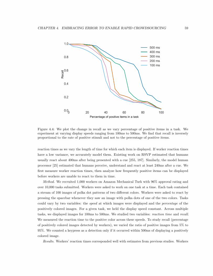
CHAPTER 4. EMBRACING ERROR TO ENABLE RAPID CROWDSOURCING 59
Figure 4.4: We plot the change in recall as we vary percentage of positive items in a task. Weexperiment at varying display speeds ranging from 100ms to 500ms. We find that recall is inverselyproportional to the rate of positive stimuli and not to the percentage of positive items.
reaction times as we vary the length of time for which each item is displayed. If worker reaction times
have a low variance, we accurately model them. Existing work on RSVP estimated that humans
usually react about 400ms after being presented with a cue [255, 187]. Similarly, the model human
processor [25] estimated that humans perceive, understand and react at least 240ms after a cue. We
first measure worker reaction times, then analyze how frequently positive items can be displayed
before workers are unable to react to them in time.
Method. We recruited 1,000 workers on Amazon Mechanical Turk with 96% approval rating and
over 10,000 tasks submitted. Workers were asked to work on one task at a time. Each task contained
a stream of 100 images of polka dot patterns of two different colors. Workers were asked to react by
pressing the spacebar whenever they saw an image with polka dots of one of the two colors. Tasks
could vary by two variables: the speed at which images were displayed and the percentage of the
positively colored images. For a given task, we held the display speed constant. Across multiple
tasks, we displayed images for 100ms to 500ms. We studied two variables: reaction time and recall.
We measured the reaction time to the positive color across these speeds. To study recall (percentage
of positively colored images detected by workers), we varied the ratio of positive images from 5% to
95%. We counted a keypress as a detection only if it occurred within 500ms of displaying a positively
colored image.
Results. Workers’ reaction times corresponded well with estimates from previous studies. Workers
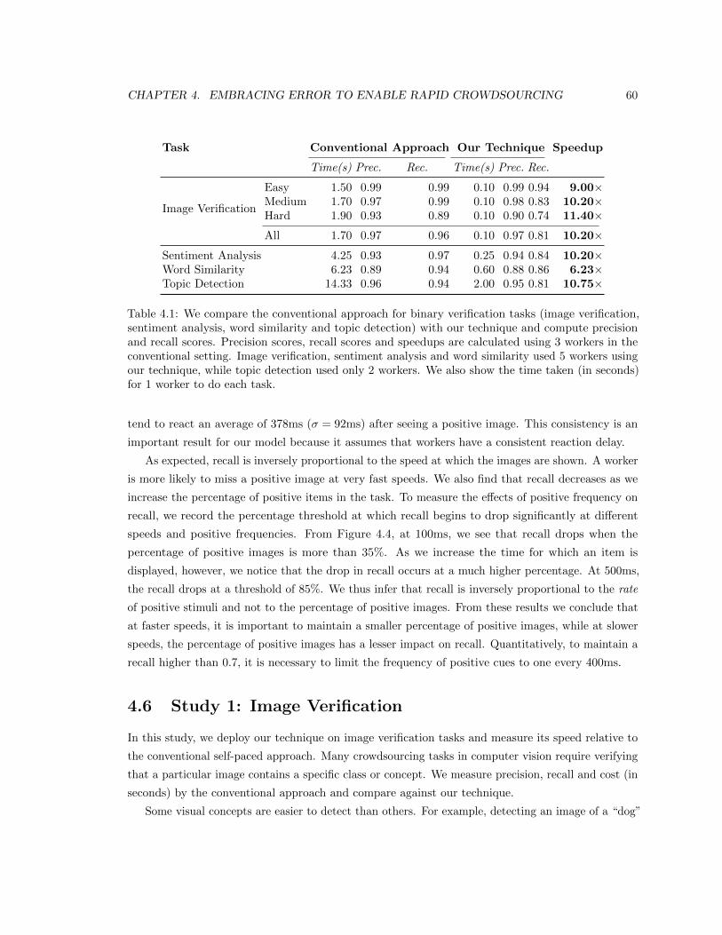
CHAPTER 4. EMBRACING ERROR TO ENABLE RAPID CROWDSOURCING 60
Task Conventional Approach Our Technique Speedup
Time(s) Prec. Rec. Time(s) Prec. Rec.
Image Verification
Easy 1.50 0.99 0.99 0.10 0.99 0.94 9.00×Medium 1.70 0.97 0.99 0.10 0.98 0.83 10.20×Hard 1.90 0.93 0.89 0.10 0.90 0.74 11.40×All 1.70 0.97 0.96 0.10 0.97 0.81 10.20×
Sentiment Analysis 4.25 0.93 0.97 0.25 0.94 0.84 10.20×Word Similarity 6.23 0.89 0.94 0.60 0.88 0.86 6.23×Topic Detection 14.33 0.96 0.94 2.00 0.95 0.81 10.75×
Table 4.1: We compare the conventional approach for binary verification tasks (image verification,sentiment analysis, word similarity and topic detection) with our technique and compute precisionand recall scores. Precision scores, recall scores and speedups are calculated using 3 workers in theconventional setting. Image verification, sentiment analysis and word similarity used 5 workers usingour technique, while topic detection used only 2 workers. We also show the time taken (in seconds)for 1 worker to do each task.
tend to react an average of 378ms (σ = 92ms) after seeing a positive image. This consistency is an
important result for our model because it assumes that workers have a consistent reaction delay.
As expected, recall is inversely proportional to the speed at which the images are shown. A worker
is more likely to miss a positive image at very fast speeds. We also find that recall decreases as we
increase the percentage of positive items in the task. To measure the effects of positive frequency on
recall, we record the percentage threshold at which recall begins to drop significantly at different
speeds and positive frequencies. From Figure 4.4, at 100ms, we see that recall drops when the
percentage of positive images is more than 35%. As we increase the time for which an item is
displayed, however, we notice that the drop in recall occurs at a much higher percentage. At 500ms,
the recall drops at a threshold of 85%. We thus infer that recall is inversely proportional to the rate
of positive stimuli and not to the percentage of positive images. From these results we conclude that
at faster speeds, it is important to maintain a smaller percentage of positive images, while at slower
speeds, the percentage of positive images has a lesser impact on recall. Quantitatively, to maintain a
recall higher than 0.7, it is necessary to limit the frequency of positive cues to one every 400ms.
4.6 Study 1: Image Verification
In this study, we deploy our technique on image verification tasks and measure its speed relative to
the conventional self-paced approach. Many crowdsourcing tasks in computer vision require verifying
that a particular image contains a specific class or concept. We measure precision, recall and cost (in
seconds) by the conventional approach and compare against our technique.
Some visual concepts are easier to detect than others. For example, detecting an image of a “dog”
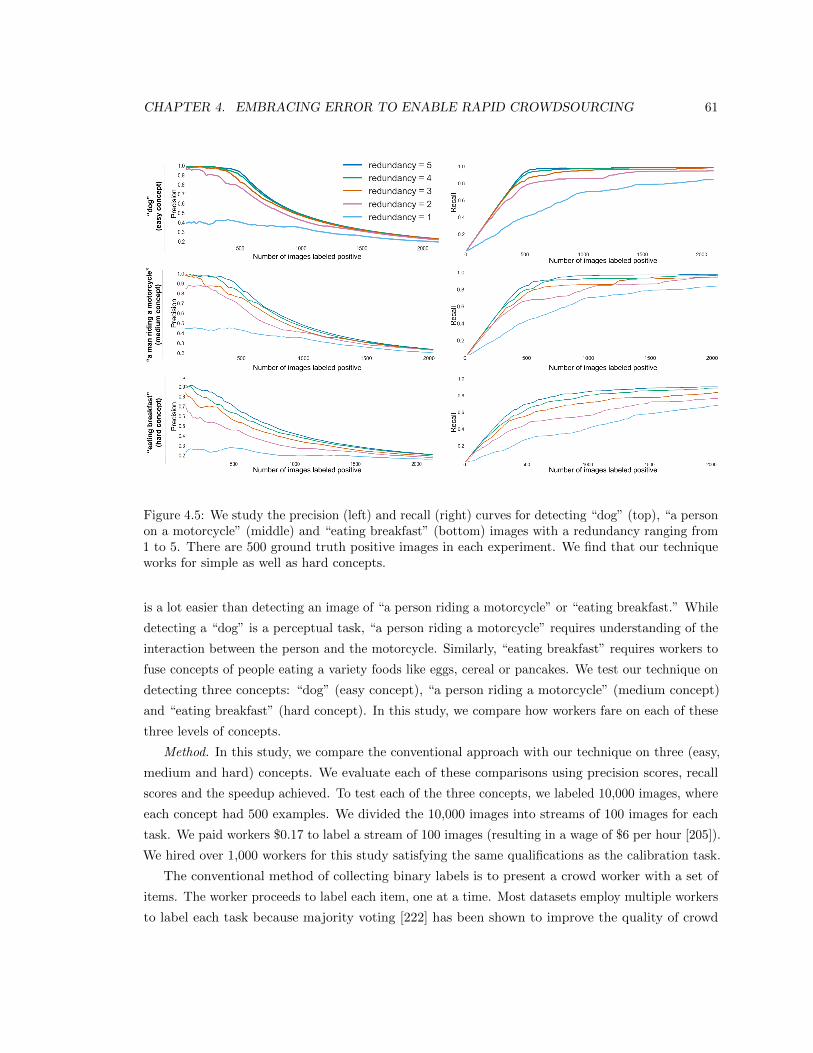
CHAPTER 4. EMBRACING ERROR TO ENABLE RAPID CROWDSOURCING 61
Figure 4.5: We study the precision (left) and recall (right) curves for detecting “dog” (top), “a personon a motorcycle” (middle) and “eating breakfast” (bottom) images with a redundancy ranging from1 to 5. There are 500 ground truth positive images in each experiment. We find that our techniqueworks for simple as well as hard concepts.
is a lot easier than detecting an image of “a person riding a motorcycle” or “eating breakfast.” While
detecting a “dog” is a perceptual task, “a person riding a motorcycle” requires understanding of the
interaction between the person and the motorcycle. Similarly, “eating breakfast” requires workers to
fuse concepts of people eating a variety foods like eggs, cereal or pancakes. We test our technique on
detecting three concepts: “dog” (easy concept), “a person riding a motorcycle” (medium concept)
and “eating breakfast” (hard concept). In this study, we compare how workers fare on each of these
three levels of concepts.
Method. In this study, we compare the conventional approach with our technique on three (easy,
medium and hard) concepts. We evaluate each of these comparisons using precision scores, recall
scores and the speedup achieved. To test each of the three concepts, we labeled 10,000 images, where
each concept had 500 examples. We divided the 10,000 images into streams of 100 images for each
task. We paid workers $0.17 to label a stream of 100 images (resulting in a wage of $6 per hour [205]).
We hired over 1,000 workers for this study satisfying the same qualifications as the calibration task.
The conventional method of collecting binary labels is to present a crowd worker with a set of
items. The worker proceeds to label each item, one at a time. Most datasets employ multiple workers
to label each task because majority voting [222] has been shown to improve the quality of crowd
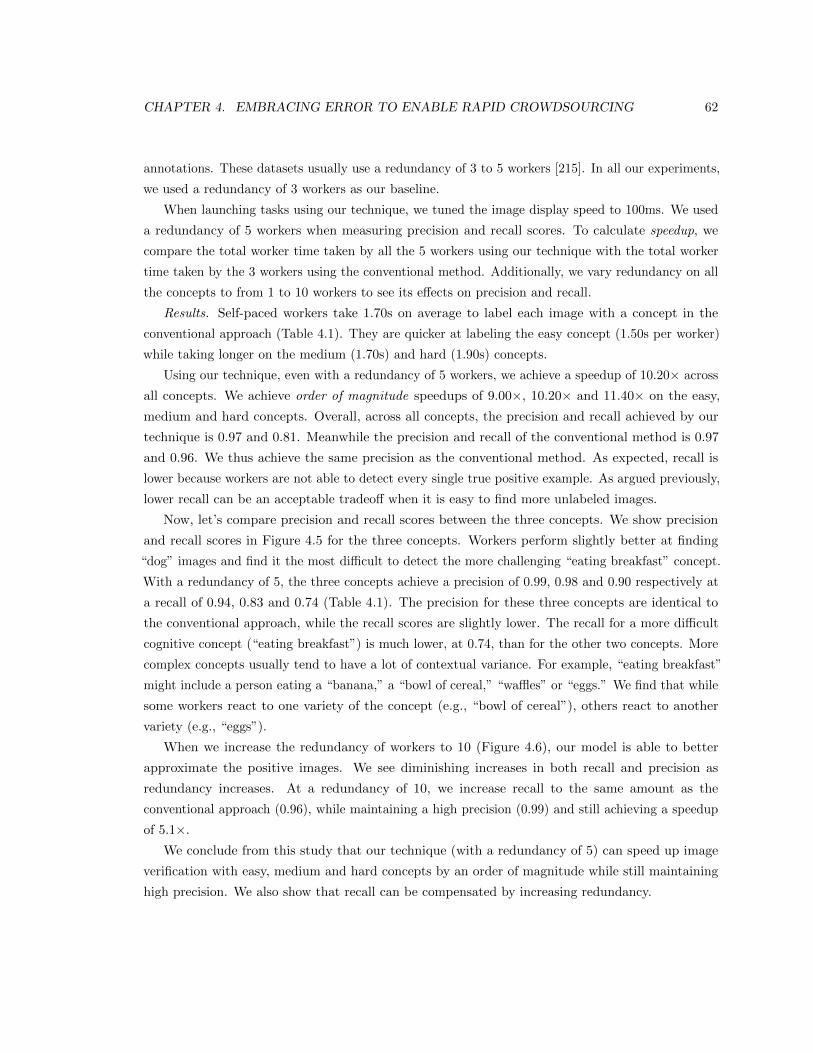
CHAPTER 4. EMBRACING ERROR TO ENABLE RAPID CROWDSOURCING 62
annotations. These datasets usually use a redundancy of 3 to 5 workers [215]. In all our experiments,
we used a redundancy of 3 workers as our baseline.
When launching tasks using our technique, we tuned the image display speed to 100ms. We used
a redundancy of 5 workers when measuring precision and recall scores. To calculate speedup, we
compare the total worker time taken by all the 5 workers using our technique with the total worker
time taken by the 3 workers using the conventional method. Additionally, we vary redundancy on all
the concepts to from 1 to 10 workers to see its effects on precision and recall.
Results. Self-paced workers take 1.70s on average to label each image with a concept in the
conventional approach (Table 4.1). They are quicker at labeling the easy concept (1.50s per worker)
while taking longer on the medium (1.70s) and hard (1.90s) concepts.
Using our technique, even with a redundancy of 5 workers, we achieve a speedup of 10.20× across
all concepts. We achieve order of magnitude speedups of 9.00×, 10.20× and 11.40× on the easy,
medium and hard concepts. Overall, across all concepts, the precision and recall achieved by our
technique is 0.97 and 0.81. Meanwhile the precision and recall of the conventional method is 0.97
and 0.96. We thus achieve the same precision as the conventional method. As expected, recall is
lower because workers are not able to detect every single true positive example. As argued previously,
lower recall can be an acceptable tradeoff when it is easy to find more unlabeled images.
Now, let’s compare precision and recall scores between the three concepts. We show precision
and recall scores in Figure 4.5 for the three concepts. Workers perform slightly better at finding
“dog” images and find it the most difficult to detect the more challenging “eating breakfast” concept.
With a redundancy of 5, the three concepts achieve a precision of 0.99, 0.98 and 0.90 respectively at
a recall of 0.94, 0.83 and 0.74 (Table 4.1). The precision for these three concepts are identical to
the conventional approach, while the recall scores are slightly lower. The recall for a more difficult
cognitive concept (“eating breakfast”) is much lower, at 0.74, than for the other two concepts. More
complex concepts usually tend to have a lot of contextual variance. For example, “eating breakfast”
might include a person eating a “banana,” a “bowl of cereal,” “waffles” or “eggs.” We find that while
some workers react to one variety of the concept (e.g., “bowl of cereal”), others react to another
variety (e.g., “eggs”).
When we increase the redundancy of workers to 10 (Figure 4.6), our model is able to better
approximate the positive images. We see diminishing increases in both recall and precision as
redundancy increases. At a redundancy of 10, we increase recall to the same amount as the
conventional approach (0.96), while maintaining a high precision (0.99) and still achieving a speedup
of 5.1×.
We conclude from this study that our technique (with a redundancy of 5) can speed up image
verification with easy, medium and hard concepts by an order of magnitude while still maintaining
high precision. We also show that recall can be compensated by increasing redundancy.
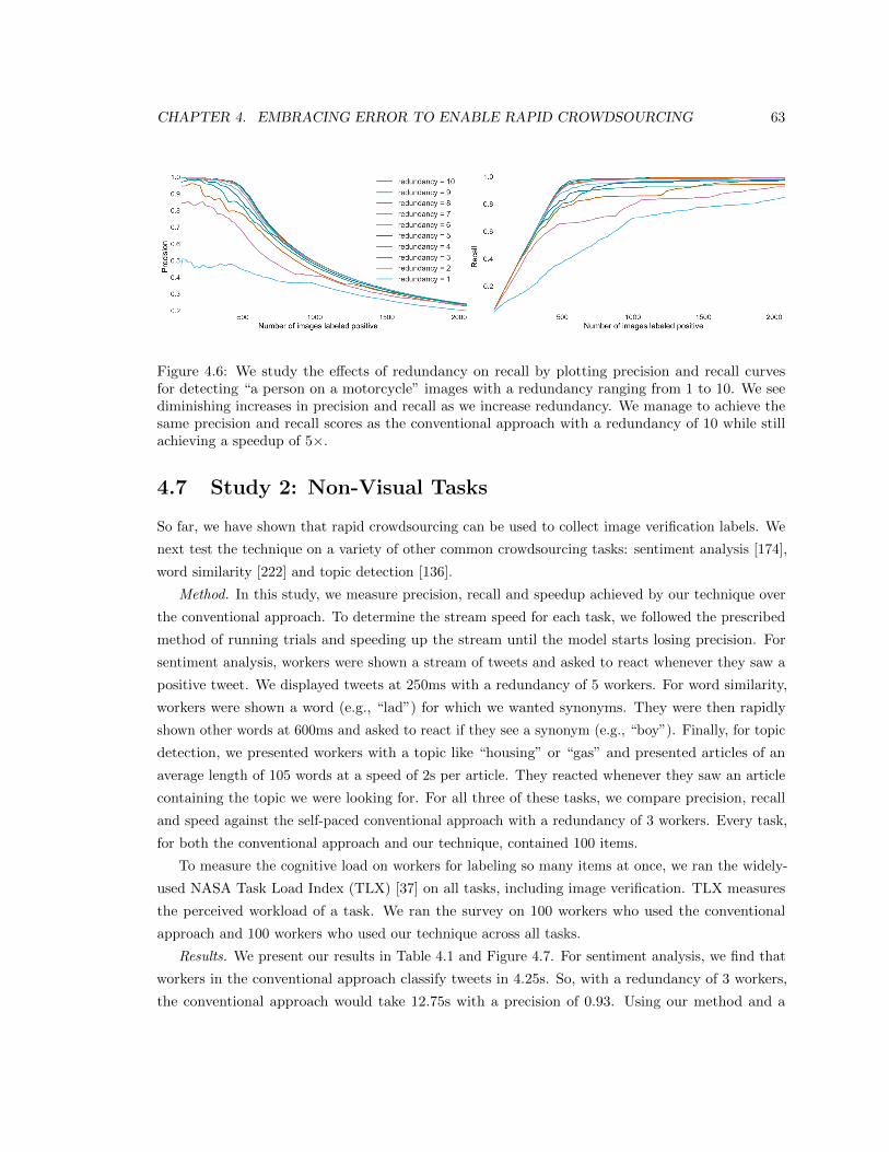
CHAPTER 4. EMBRACING ERROR TO ENABLE RAPID CROWDSOURCING 63
Figure 4.6: We study the effects of redundancy on recall by plotting precision and recall curvesfor detecting “a person on a motorcycle” images with a redundancy ranging from 1 to 10. We seediminishing increases in precision and recall as we increase redundancy. We manage to achieve thesame precision and recall scores as the conventional approach with a redundancy of 10 while stillachieving a speedup of 5×.
4.7 Study 2: Non-Visual Tasks
So far, we have shown that rapid crowdsourcing can be used to collect image verification labels. We
next test the technique on a variety of other common crowdsourcing tasks: sentiment analysis [174],
word similarity [222] and topic detection [136].
Method. In this study, we measure precision, recall and speedup achieved by our technique over
the conventional approach. To determine the stream speed for each task, we followed the prescribed
method of running trials and speeding up the stream until the model starts losing precision. For
sentiment analysis, workers were shown a stream of tweets and asked to react whenever they saw a
positive tweet. We displayed tweets at 250ms with a redundancy of 5 workers. For word similarity,
workers were shown a word (e.g., “lad”) for which we wanted synonyms. They were then rapidly
shown other words at 600ms and asked to react if they see a synonym (e.g., “boy”). Finally, for topic
detection, we presented workers with a topic like “housing” or “gas” and presented articles of an
average length of 105 words at a speed of 2s per article. They reacted whenever they saw an article
containing the topic we were looking for. For all three of these tasks, we compare precision, recall
and speed against the self-paced conventional approach with a redundancy of 3 workers. Every task,
for both the conventional approach and our technique, contained 100 items.
To measure the cognitive load on workers for labeling so many items at once, we ran the widely-
used NASA Task Load Index (TLX) [37] on all tasks, including image verification. TLX measures
the perceived workload of a task. We ran the survey on 100 workers who used the conventional
approach and 100 workers who used our technique across all tasks.
Results. We present our results in Table 4.1 and Figure 4.7. For sentiment analysis, we find that
workers in the conventional approach classify tweets in 4.25s. So, with a redundancy of 3 workers,
the conventional approach would take 12.75s with a precision of 0.93. Using our method and a
CHAPTER 4. EMBRACING ERROR TO ENABLE RAPID CROWDSOURCING 64
redundancy of 5 workers, we complete the task in 1250ms (250ms per worker per item) and 0.94
precision. Therefore, our technique achieves a speedup of 10.2×.
Likewise, for word similarity, workers take around 6.23s to complete the conventional task, while
our technique succeeds at 600ms. We manage to capture a comparable precision of 0.88 using 5
workers against a precision of 0.89 in the conventional method with 3 workers. Since finding synonyms
is a higher-level cognitive task, workers take longer to do word similarity tasks than image verification
and sentiment analysis tasks. We manage a speedup of 6.23×.
Finally, for topic detection, workers spend significant time analyzing articles in the conventional
setting (14.33s on average). With 3 workers, the conventional approach takes 43s. In comparison, our
technique delegates 2s for each article. With a redundancy of only 2 workers, we achieve a precision
of 0.95, similar to the 0.96 achieved by the conventional approach. The total worker time to label
one article using our technique is 4s, a speedup of 10.75×.
The mean TLX workload for the control condition was 58.5 (σ = 9.3), and 62.4 (σ = 18.5) for our
technique. Unexpectedly, the difference between conditions was not significant (t(99) = −0.53, p =
0.59). The temporal demand scale item appeared to be elevated for our technique (61.1 vs. 70.0),
but this difference was not significant (t(99) = −0.76, p = 0.45). We conclude that our technique can
be used to scale crowdsourcing on a variety of tasks without statistically increasing worker workload.
4.8 Study 3: Multi-class Classification
In this study, we extend our technique from binary to multi-class classification to capture an even
larger set of crowdsourcing tasks. We use our technique to create a dataset where each image is
classified into one category (“people,” “dog,” “horse,” “cat,” etc.). We compare our technique with a
conventional technique [43] that collects binary labels for each image for every single possible class.
Method. Our aim is to classify a dataset of 2,000 images with 10 categories where each category
contains between 100 to 250 examples. We compared three methods of multi-class classification: (1)
a naive approach that collected 10 binary labels (one for each class) for each image, (2) a baseline
approach that used our interface and classified images one class (chosen randomly) at a time, and (3)
a class-optimized approach that used our interface to classify images starting from the class with the
most examples. When using our interface, we broke tasks into streams of 100 images displayed for
100ms each. We used a redundancy of 3 workers for the conventional interface and 5 workers for our
interface. We calculated the precision and recall scores across each of these three methods as well as
the cost (in seconds) of each method.
Results. (1) In the naive approach, we need to collect 20,000 binary labels that take 1.7s each.
With 5 workers, this takes 102,000s ($170 at a wage rate of $6/hr) with an average precision of
0.99 and recall of 0.95. (2) Using the baseline approach, it takes 12,342s ($20.57) with an average
precision of 0.98 and recall of 0.83. This shows that the baseline approach achieves a speedup of
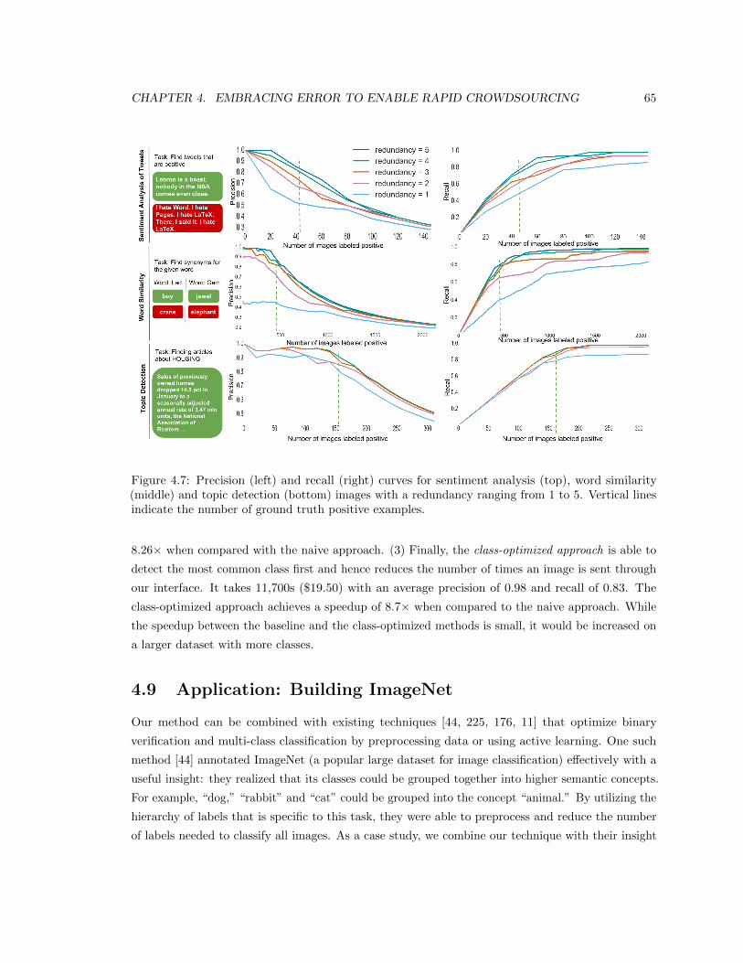
CHAPTER 4. EMBRACING ERROR TO ENABLE RAPID CROWDSOURCING 65
Figure 4.7: Precision (left) and recall (right) curves for sentiment analysis (top), word similarity(middle) and topic detection (bottom) images with a redundancy ranging from 1 to 5. Vertical linesindicate the number of ground truth positive examples.
8.26× when compared with the naive approach. (3) Finally, the class-optimized approach is able to
detect the most common class first and hence reduces the number of times an image is sent through
our interface. It takes 11,700s ($19.50) with an average precision of 0.98 and recall of 0.83. The
class-optimized approach achieves a speedup of 8.7× when compared to the naive approach. While
the speedup between the baseline and the class-optimized methods is small, it would be increased on
a larger dataset with more classes.
4.9 Application: Building ImageNet
Our method can be combined with existing techniques [44, 225, 176, 11] that optimize binary
verification and multi-class classification by preprocessing data or using active learning. One such
method [44] annotated ImageNet (a popular large dataset for image classification) effectively with a
useful insight: they realized that its classes could be grouped together into higher semantic concepts.
For example, “dog,” “rabbit” and “cat” could be grouped into the concept “animal.” By utilizing the
hierarchy of labels that is specific to this task, they were able to preprocess and reduce the number
of labels needed to classify all images. As a case study, we combine our technique with their insight
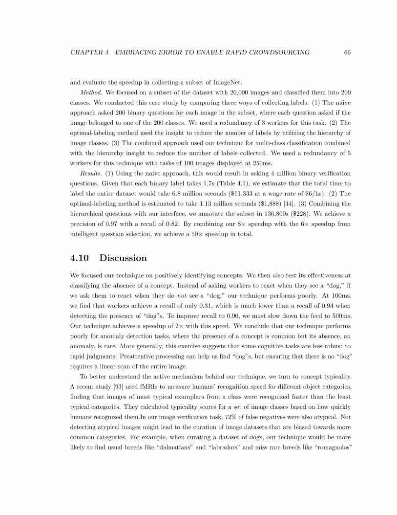
CHAPTER 4. EMBRACING ERROR TO ENABLE RAPID CROWDSOURCING 66
and evaluate the speedup in collecting a subset of ImageNet.
Method. We focused on a subset of the dataset with 20,000 images and classified them into 200
classes. We conducted this case study by comparing three ways of collecting labels: (1) The naive
approach asked 200 binary questions for each image in the subset, where each question asked if the
image belonged to one of the 200 classes. We used a redundancy of 3 workers for this task. (2) The
optimal-labeling method used the insight to reduce the number of labels by utilizing the hierarchy of
image classes. (3) The combined approach used our technique for multi-class classification combined
with the hierarchy insight to reduce the number of labels collected. We used a redundancy of 5
workers for this technique with tasks of 100 images displayed at 250ms.
Results. (1) Using the naive approach, this would result in asking 4 million binary verification
questions. Given that each binary label takes 1.7s (Table 4.1), we estimate that the total time to
label the entire dataset would take 6.8 million seconds ($11,333 at a wage rate of $6/hr). (2) The
optimal-labeling method is estimated to take 1.13 million seconds ($1,888) [44]. (3) Combining the
hierarchical questions with our interface, we annotate the subset in 136,800s ($228). We achieve a
precision of 0.97 with a recall of 0.82. By combining our 8× speedup with the 6× speedup from
intelligent question selection, we achieve a 50× speedup in total.
4.10 Discussion
We focused our technique on positively identifying concepts. We then also test its effectiveness at
classifying the absence of a concept. Instead of asking workers to react when they see a “dog,” if
we ask them to react when they do not see a “dog,” our technique performs poorly. At 100ms,
we find that workers achieve a recall of only 0.31, which is much lower than a recall of 0.94 when
detecting the presence of “dog”s. To improve recall to 0.90, we must slow down the feed to 500ms.
Our technique achieves a speedup of 2× with this speed. We conclude that our technique performs
poorly for anomaly detection tasks, where the presence of a concept is common but its absence, an
anomaly, is rare. More generally, this exercise suggests that some cognitive tasks are less robust to
rapid judgments. Preattentive processing can help us find “dog”s, but ensuring that there is no “dog”
requires a linear scan of the entire image.
To better understand the active mechanism behind our technique, we turn to concept typicality.
A recent study [93] used fMRIs to measure humans’ recognition speed for different object categories,
finding that images of most typical examplars from a class were recognized faster than the least
typical categories. They calculated typicality scores for a set of image classes based on how quickly
humans recognized them.In our image verification task, 72% of false negatives were also atypical. Not
detecting atypical images might lead to the curation of image datasets that are biased towards more
common categories. For example, when curating a dataset of dogs, our technique would be more
likely to find usual breeds like “dalmatians” and “labradors” and miss rare breeds like “romagnolos”
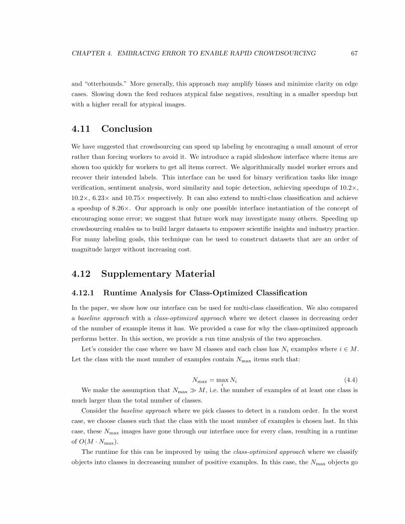
CHAPTER 4. EMBRACING ERROR TO ENABLE RAPID CROWDSOURCING 67
and “otterhounds.” More generally, this approach may amplify biases and minimize clarity on edge
cases. Slowing down the feed reduces atypical false negatives, resulting in a smaller speedup but
with a higher recall for atypical images.
4.11 Conclusion
We have suggested that crowdsourcing can speed up labeling by encouraging a small amount of error
rather than forcing workers to avoid it. We introduce a rapid slideshow interface where items are
shown too quickly for workers to get all items correct. We algorithmically model worker errors and
recover their intended labels. This interface can be used for binary verification tasks like image
verification, sentiment analysis, word similarity and topic detection, achieving speedups of 10.2×,
10.2×, 6.23× and 10.75× respectively. It can also extend to multi-class classification and achieve
a speedup of 8.26×. Our approach is only one possible interface instantiation of the concept of
encouraging some error; we suggest that future work may investigate many others. Speeding up
crowdsourcing enables us to build larger datasets to empower scientific insights and industry practice.
For many labeling goals, this technique can be used to construct datasets that are an order of
magnitude larger without increasing cost.
4.12 Supplementary Material
4.12.1 Runtime Analysis for Class-Optimized Classification
In the paper, we show how our interface can be used for multi-class classification. We also compared
a baseline approach with a class-optimized approach where we detect classes in decreasing order
of the number of example items it has. We provided a case for why the class-optimized approach
performs better. In this section, we provide a run time analysis of the two approaches.
Let’s consider the case where we have M classes and each class has Ni examples where i ∈ M .
Let the class with the most number of examples contain Nmax items such that:
Nmax = maxiNi (4.4)
We make the assumption that Nmax � M , i.e. the number of examples of at least one class is
much larger than the total number of classes.
Consider the baseline approach where we pick classes to detect in a random order. In the worst
case, we choose classes such that the class with the most number of examples is chosen last. In this
case, these Nmax images have gone through our interface once for every class, resulting in a runtime
of O(M ·Nmax).
The runtime for this can be improved by using the class-optimized approach where we classify
objects into classes in decreaseing number of positive examples. In this case, the Nmax objects go

CHAPTER 4. EMBRACING ERROR TO ENABLE RAPID CROWDSOURCING 68
through our interface at the very beginning only once and get classified. Assuming Nmax � Nj∀j ∈M ,
this results in a runtime of O(Nmax). We conclude that the class-optimized approach achieves linear
time versus quadratic.
Chapter 5
Long-Term Crowd Worker Quality
5.1 Introduction
Microtask crowdsourcing is gaining popularity among corporate and research communities as a
means to leverage parallel human computation for extremely large problems [233, 8, 7, 131, 129].
These communities use crowd work to complete hundreds of thousands of tasks per day [151], from
which new datasets with over 20 million annotations can be produced within a few months [118]. A
crowdsourcing platform like Amazon’s Mechanical Turk (AMT) is a marketplace subject to human
factors that affect its performance, both in terms of speed and quality [47]. Prior studies found that
work division in crowdsourcing follows a Pareto principle, where a small minority of workers usually
completes a great majority of the work [141]. If such large crowdsourced projects are being completed
by a small percentage of workers, then these workers spend hours, days, or weeks executing the exact
same tasks. Consequently, we pose the question:
How does a worker’s quality change over time?
Multiple arguments from previous literature in psychology suggest that quality should decrease
over time. Fatigue, a temporary decline in cognitive or physical condition, can gradually result in
performance drops over long periods of time [179, 13, 122]. Since the microtask paradigm in large
scale crowdsourcing involves monotonous sequences of repetitive tasks, fatigue buildup can pose a
potential problem to the quality of submitted work over time [39]. Furthermore, workers have been
noted to be “satisficers” who, as they gain familiarity with the task and its acceptance thresholds,
strive to do the minimal work possible to achieve these thresholds [217, 27].
To study these long term effects on crowd work, we analyze worker trends over three different
real-world, large-scale datasets [118] collected from microtasks on AMT: image descriptions, question
answering, and binary verifications. With microtasks comprising over 60% of the total crowd work
and microtasks involving images being the most common type [87], these datasets cover a large
I am the main contributor on this study of long-term workers, being involved in every part of this study.
69
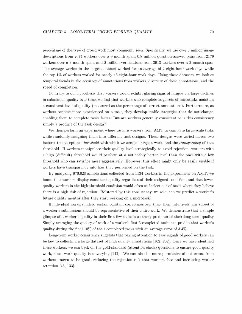
CHAPTER 5. LONG-TERM CROWD WORKER QUALITY 70
percentage of the type of crowd work most commonly seen. Specifically, we use over 5 million image
descriptions from 2674 workers over a 9 month span, 0.8 million question-answer pairs from 2179
workers over a 3 month span, and 2 million verifications from 3913 workers over a 3 month span.
The average worker in the largest dataset worked for an average of 2 eight-hour work days while
the top 1% of workers worked for nearly 45 eight-hour work days. Using these datasets, we look at
temporal trends in the accuracy of annotations from workers, diversity of these annotations, and the
speed of completion.
Contrary to our hypothesis that workers would exhibit glaring signs of fatigue via large declines
in submission quality over time, we find that workers who complete large sets of microtasks maintain
a consistent level of quality (measured as the percentage of correct annotations). Furthermore, as
workers become more experienced on a task, they develop stable strategies that do not change,
enabling them to complete tasks faster. But are workers generally consistent or is this consistency
simply a product of the task design?
We thus perform an experiment where we hire workers from AMT to complete large-scale tasks
while randomly assigning them into different task designs. These designs were varied across two
factors: the acceptance threshold with which we accept or reject work, and the transparency of that
threshold. If workers manipulate their quality level strategically to avoid rejection, workers with
a high (difficult) threshold would perform at a noticeably better level than the ones with a low
threshold who can satisfice more aggressively. However, this effect might only be easily visible if
workers have transparency into how they performed on the task.
By analyzing 676,628 annotations collected from 1134 workers in the experiment on AMT, we
found that workers display consistent quality regardless of their assigned condition, and that lower-
quality workers in the high threshold condition would often self-select out of tasks where they believe
there is a high risk of rejection. Bolstered by this consistency, we ask: can we predict a worker’s
future quality months after they start working on a microtask?
If individual workers indeed sustain constant correctness over time, then, intuitively, any subset of
a worker’s submissions should be representative of their entire work. We demonstrate that a simple
glimpse of a worker’s quality in their first few tasks is a strong predictor of their long-term quality.
Simply averaging the quality of work of a worker’s first 5 completed tasks can predict that worker’s
quality during the final 10% of their completed tasks with an average error of 3.4%.
Long-term worker consistency suggests that paying attention to easy signals of good workers can
be key to collecting a large dataset of high quality annotations [162, 202]. Once we have identified
these workers, we can back off the gold-standard (attention check) questions to ensure good quality
work, since work quality is unvarying [142]. We can also be more permissive about errors from
workers known to be good, reducing the rejection risk that workers face and increasing worker
retention [46, 133].
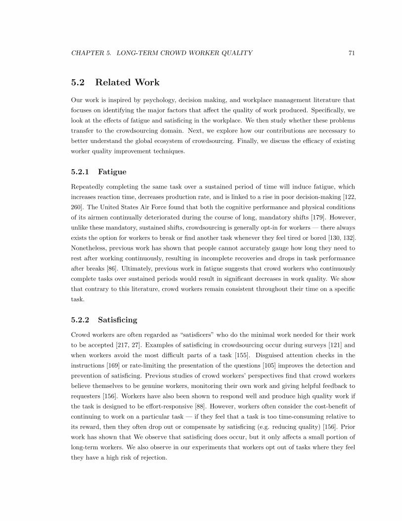
CHAPTER 5. LONG-TERM CROWD WORKER QUALITY 71
5.2 Related Work
Our work is inspired by psychology, decision making, and workplace management literature that
focuses on identifying the major factors that affect the quality of work produced. Specifically, we
look at the effects of fatigue and satisficing in the workplace. We then study whether these problems
transfer to the crowdsourcing domain. Next, we explore how our contributions are necessary to
better understand the global ecosystem of crowdsourcing. Finally, we discuss the efficacy of existing
worker quality improvement techniques.
5.2.1 Fatigue
Repeatedly completing the same task over a sustained period of time will induce fatigue, which
increases reaction time, decreases production rate, and is linked to a rise in poor decision-making [122,
260]. The United States Air Force found that both the cognitive performance and physical conditions
of its airmen continually deteriorated during the course of long, mandatory shifts [179]. However,
unlike these mandatory, sustained shifts, crowdsourcing is generally opt-in for workers — there always
exists the option for workers to break or find another task whenever they feel tired or bored [130, 132].
Nonetheless, previous work has shown that people cannot accurately gauge how long they need to
rest after working continuously, resulting in incomplete recoveries and drops in task performance
after breaks [86]. Ultimately, previous work in fatigue suggests that crowd workers who continuously
complete tasks over sustained periods would result in significant decreases in work quality. We show
that contrary to this literature, crowd workers remain consistent throughout their time on a specific
task.
5.2.2 Satisficing
Crowd workers are often regarded as “satisficers” who do the minimal work needed for their work
to be accepted [217, 27]. Examples of satisficing in crowdsourcing occur during surveys [121] and
when workers avoid the most difficult parts of a task [155]. Disguised attention checks in the
instructions [169] or rate-limiting the presentation of the questions [105] improves the detection and
prevention of satisficing. Previous studies of crowd workers’ perspectives find that crowd workers
believe themselves to be genuine workers, monitoring their own work and giving helpful feedback to
requesters [156]. Workers have also been shown to respond well and produce high quality work if
the task is designed to be effort-responsive [88]. However, workers often consider the cost-benefit of
continuing to work on a particular task — if they feel that a task is too time-consuming relative to
its reward, then they often drop out or compensate by satisficing (e.g. reducing quality) [156]. Prior
work has shown that We observe that satisficing does occur, but it only affects a small portion of
long-term workers. We also observe in our experiments that workers opt out of tasks where they feel
they have a high risk of rejection.
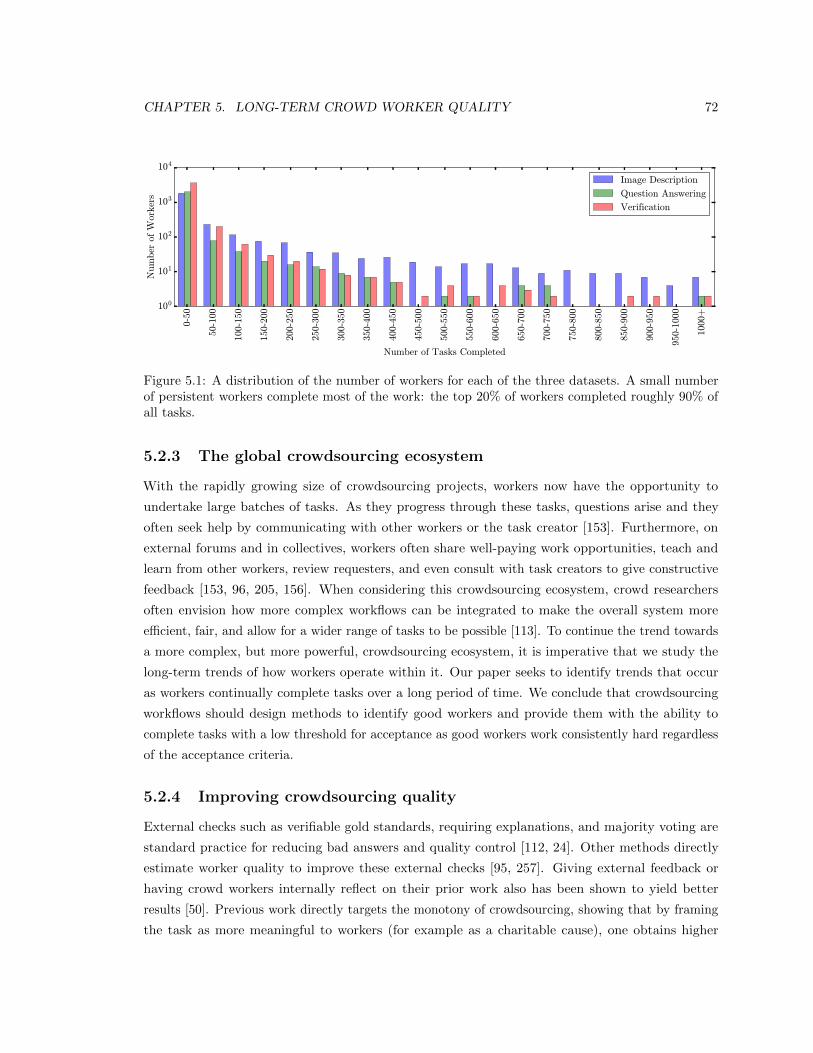
CHAPTER 5. LONG-TERM CROWD WORKER QUALITY 72
0-5
0
50-
100
100-
150
150-
200
200-
250
250-
300
300-
350
350-
400
400-
450
450-
500
500-
550
550-
600
600-
650
650-
700
700-
750
750-
800
800-
850
850-
900
900-
950
950-1
000
1000
+
Number of Tasks Completed
100
101
102
103
104
Num
ber
of W
ork
ers
Image Description
Question Answering
Verification
Figure 5.1: A distribution of the number of workers for each of the three datasets. A small numberof persistent workers complete most of the work: the top 20% of workers completed roughly 90% ofall tasks.
5.2.3 The global crowdsourcing ecosystem
With the rapidly growing size of crowdsourcing projects, workers now have the opportunity to
undertake large batches of tasks. As they progress through these tasks, questions arise and they
often seek help by communicating with other workers or the task creator [153]. Furthermore, on
external forums and in collectives, workers often share well-paying work opportunities, teach and
learn from other workers, review requesters, and even consult with task creators to give constructive
feedback [153, 96, 205, 156]. When considering this crowdsourcing ecosystem, crowd researchers
often envision how more complex workflows can be integrated to make the overall system more
efficient, fair, and allow for a wider range of tasks to be possible [113]. To continue the trend towards
a more complex, but more powerful, crowdsourcing ecosystem, it is imperative that we study the
long-term trends of how workers operate within it. Our paper seeks to identify trends that occur
as workers continually complete tasks over a long period of time. We conclude that crowdsourcing
workflows should design methods to identify good workers and provide them with the ability to
complete tasks with a low threshold for acceptance as good workers work consistently hard regardless
of the acceptance criteria.
5.2.4 Improving crowdsourcing quality
External checks such as verifiable gold standards, requiring explanations, and majority voting are
standard practice for reducing bad answers and quality control [112, 24]. Other methods directly
estimate worker quality to improve these external checks [95, 257]. Giving external feedback or
having crowd workers internally reflect on their prior work also has been shown to yield better
results [50]. Previous work directly targets the monotony of crowdsourcing, showing that by framing
the task as more meaningful to workers (for example as a charitable cause), one obtains higher
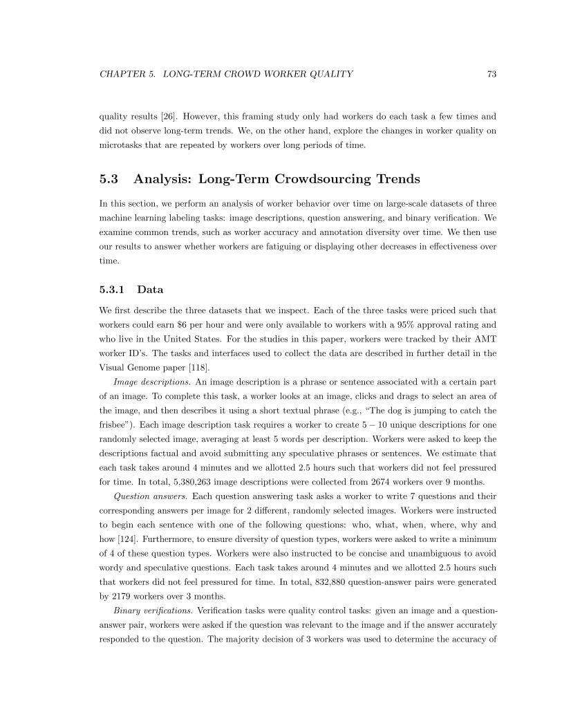
CHAPTER 5. LONG-TERM CROWD WORKER QUALITY 73
quality results [26]. However, this framing study only had workers do each task a few times and
did not observe long-term trends. We, on the other hand, explore the changes in worker quality on
microtasks that are repeated by workers over long periods of time.
5.3 Analysis: Long-Term Crowdsourcing Trends
In this section, we perform an analysis of worker behavior over time on large-scale datasets of three
machine learning labeling tasks: image descriptions, question answering, and binary verification. We
examine common trends, such as worker accuracy and annotation diversity over time. We then use
our results to answer whether workers are fatiguing or displaying other decreases in effectiveness over
time.
5.3.1 Data
We first describe the three datasets that we inspect. Each of the three tasks were priced such that
workers could earn $6 per hour and were only available to workers with a 95% approval rating and
who live in the United States. For the studies in this paper, workers were tracked by their AMT
worker ID’s. The tasks and interfaces used to collect the data are described in further detail in the
Visual Genome paper [118].
Image descriptions. An image description is a phrase or sentence associated with a certain part
of an image. To complete this task, a worker looks at an image, clicks and drags to select an area of
the image, and then describes it using a short textual phrase (e.g., “The dog is jumping to catch the
frisbee”). Each image description task requires a worker to create 5− 10 unique descriptions for one
randomly selected image, averaging at least 5 words per description. Workers were asked to keep the
descriptions factual and avoid submitting any speculative phrases or sentences. We estimate that
each task takes around 4 minutes and we allotted 2.5 hours such that workers did not feel pressured
for time. In total, 5,380,263 image descriptions were collected from 2674 workers over 9 months.
Question answers. Each question answering task asks a worker to write 7 questions and their
corresponding answers per image for 2 different, randomly selected images. Workers were instructed
to begin each sentence with one of the following questions: who, what, when, where, why and
how [124]. Furthermore, to ensure diversity of question types, workers were asked to write a minimum
of 4 of these question types. Workers were also instructed to be concise and unambiguous to avoid
wordy and speculative questions. Each task takes around 4 minutes and we allotted 2.5 hours such
that workers did not feel pressured for time. In total, 832,880 question-answer pairs were generated
by 2179 workers over 3 months.
Binary verifications. Verification tasks were quality control tasks: given an image and a question-
answer pair, workers were asked if the question was relevant to the image and if the answer accurately
responded to the question. The majority decision of 3 workers was used to determine the accuracy of
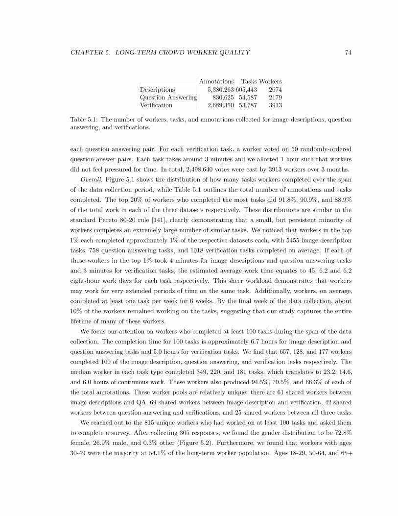
CHAPTER 5. LONG-TERM CROWD WORKER QUALITY 74
Annotations Tasks Workers
Descriptions 5,380,263 605,443 2674Question Answering 830,625 54,587 2179Verification 2,689,350 53,787 3913
Table 5.1: The number of workers, tasks, and annotations collected for image descriptions, questionanswering, and verifications.
each question answering pair. For each verification task, a worker voted on 50 randomly-ordered
question-answer pairs. Each task takes around 3 minutes and we allotted 1 hour such that workers
did not feel pressured for time. In total, 2,498,640 votes were cast by 3913 workers over 3 months.
Overall. Figure 5.1 shows the distribution of how many tasks workers completed over the span
of the data collection period, while Table 5.1 outlines the total number of annotations and tasks
completed. The top 20% of workers who completed the most tasks did 91.8%, 90.9%, and 88.9%
of the total work in each of the three datasets respectively. These distributions are similar to the
standard Pareto 80-20 rule [141], clearly demonstrating that a small, but persistent minority of
workers completes an extremely large number of similar tasks. We noticed that workers in the top
1% each completed approximately 1% of the respective datasets each, with 5455 image description
tasks, 758 question answering tasks, and 1018 verification tasks completed on average. If each of
these workers in the top 1% took 4 minutes for image descriptions and question answering tasks
and 3 minutes for verification tasks, the estimated average work time equates to 45, 6.2 and 6.2
eight-hour work days for each task respectively. This sheer workload demonstrates that workers
may work for very extended periods of time on the same task. Additionally, workers, on average,
completed at least one task per week for 6 weeks. By the final week of the data collection, about
10% of the workers remained working on the tasks, suggesting that our study captures the entire
lifetime of many of these workers.
We focus our attention on workers who completed at least 100 tasks during the span of the data
collection. The completion time for 100 tasks is approximately 6.7 hours for image description and
question answering tasks and 5.0 hours for verification tasks. We find that 657, 128, and 177 workers
completed 100 of the image description, question answering, and verification tasks respectively. The
median worker in each task type completed 349, 220, and 181 tasks, which translates to 23.2, 14.6,
and 6.0 hours of continuous work. These workers also produced 94.5%, 70.5%, and 66.3% of each of
the total annotations. These worker pools are relatively unique: there are 61 shared workers between
image descriptions and QA, 69 shared workers between image description and verification, 42 shared
workers between question answering and verifications, and 25 shared workers between all three tasks.
We reached out to the 815 unique workers who had worked on at least 100 tasks and asked them
to complete a survey. After collecting 305 responses, we found the gender distribution to be 72.8%
female, 26.9% male, and 0.3% other (Figure 5.2). Furthermore, we found that workers with ages
30-49 were the majority at 54.1% of the long-term worker population. Ages 18-29, 50-64, and 65+
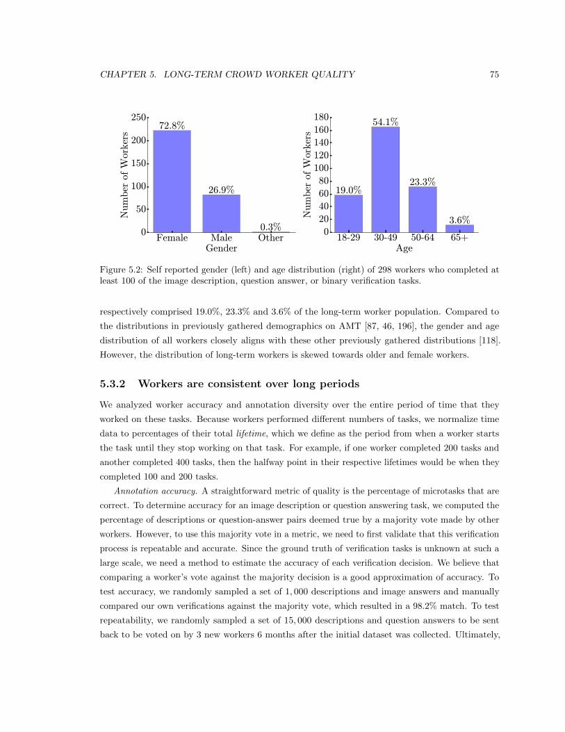
CHAPTER 5. LONG-TERM CROWD WORKER QUALITY 75
Female Male OtherGender
0
50
100
150
200
250N
um
ber
of W
orker
s72.8%
26.9%
0.3%18-29 30-49 50-64 65+
Age
0
20
40
60
80
100
120
140
160
180
Num
ber
of W
ork
ers
19.0%
54.1%
23.3%
3.6%
Figure 5.2: Self reported gender (left) and age distribution (right) of 298 workers who completed atleast 100 of the image description, question answer, or binary verification tasks.
respectively comprised 19.0%, 23.3% and 3.6% of the long-term worker population. Compared to
the distributions in previously gathered demographics on AMT [87, 46, 196], the gender and age
distribution of all workers closely aligns with these other previously gathered distributions [118].
However, the distribution of long-term workers is skewed towards older and female workers.
5.3.2 Workers are consistent over long periods
We analyzed worker accuracy and annotation diversity over the entire period of time that they
worked on these tasks. Because workers performed different numbers of tasks, we normalize time
data to percentages of their total lifetime, which we define as the period from when a worker starts
the task until they stop working on that task. For example, if one worker completed 200 tasks and
another completed 400 tasks, then the halfway point in their respective lifetimes would be when they
completed 100 and 200 tasks.
Annotation accuracy. A straightforward metric of quality is the percentage of microtasks that are
correct. To determine accuracy for an image description or question answering task, we computed the
percentage of descriptions or question-answer pairs deemed true by a majority vote made by other
workers. However, to use this majority vote in a metric, we need to first validate that this verification
process is repeatable and accurate. Since the ground truth of verification tasks is unknown at such a
large scale, we need a method to estimate the accuracy of each verification decision. We believe that
comparing a worker’s vote against the majority decision is a good approximation of accuracy. To
test accuracy, we randomly sampled a set of 1, 000 descriptions and image answers and manually
compared our own verifications against the majority vote, which resulted in a 98.2% match. To test
repeatability, we randomly sampled a set of 15, 000 descriptions and question answers to be sent
back to be voted on by 3 new workers 6 months after the initial dataset was collected. Ultimately,
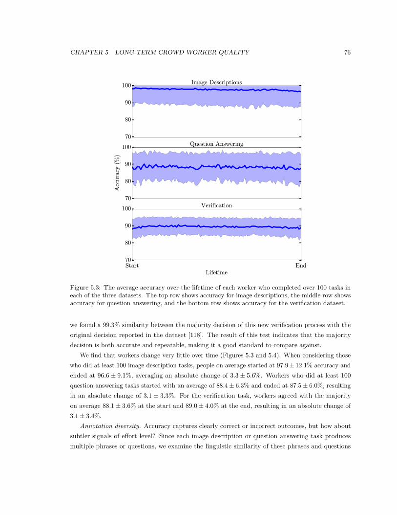
CHAPTER 5. LONG-TERM CROWD WORKER QUALITY 76
70
80
90
100 Image Descriptions
70
80
90
100
Acc
ura
cy (
%)
Question Answering
Start EndLifetime
70
80
90
100 Verification
Figure 5.3: The average accuracy over the lifetime of each worker who completed over 100 tasks ineach of the three datasets. The top row shows accuracy for image descriptions, the middle row showsaccuracy for question answering, and the bottom row shows accuracy for the verification dataset.
we found a 99.3% similarity between the majority decision of this new verification process with the
original decision reported in the dataset [118]. The result of this test indicates that the majority
decision is both accurate and repeatable, making it a good standard to compare against.
We find that workers change very little over time (Figures 5.3 and 5.4). When considering those
who did at least 100 image description tasks, people on average started at 97.9± 12.1% accuracy and
ended at 96.6 ± 9.1%, averaging an absolute change of 3.3 ± 5.6%. Workers who did at least 100
question answering tasks started with an average of 88.4± 6.3% and ended at 87.5± 6.0%, resulting
in an absolute change of 3.1 ± 3.3%. For the verification task, workers agreed with the majority
on average 88.1± 3.6% at the start and 89.0± 4.0% at the end, resulting in an absolute change of
3.1± 3.4%.
Annotation diversity. Accuracy captures clearly correct or incorrect outcomes, but how about
subtler signals of effort level? Since each image description or question answering task produces
multiple phrases or questions, we examine the linguistic similarity of these phrases and questions
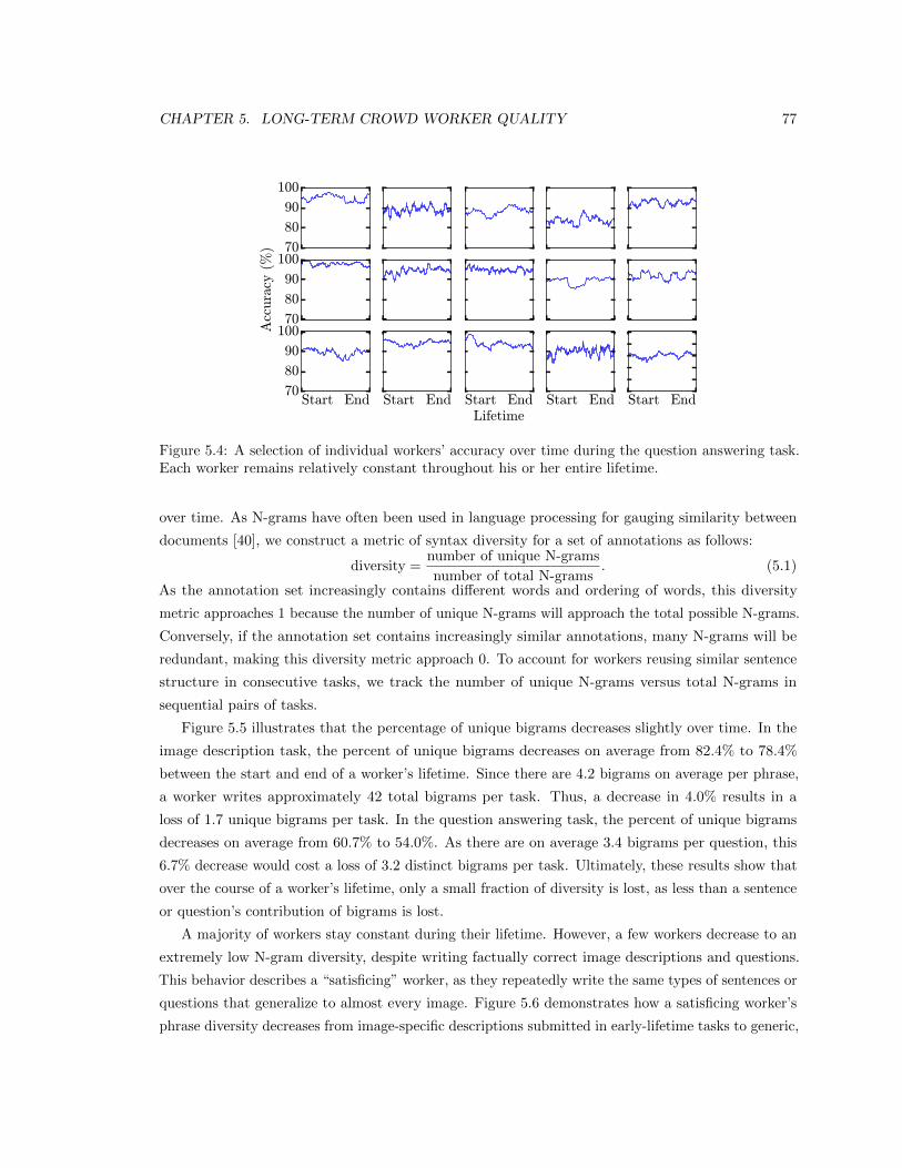
CHAPTER 5. LONG-TERM CROWD WORKER QUALITY 77
70
80
90
100
70
80
90
100A
ccura
cy (
%)
Start End70
80
90
100
Start End Start EndLifetime
Start End Start End
Figure 5.4: A selection of individual workers’ accuracy over time during the question answering task.Each worker remains relatively constant throughout his or her entire lifetime.
over time. As N-grams have often been used in language processing for gauging similarity between
documents [40], we construct a metric of syntax diversity for a set of annotations as follows:
diversity =number of unique N-grams
number of total N-grams. (5.1)
As the annotation set increasingly contains different words and ordering of words, this diversity
metric approaches 1 because the number of unique N-grams will approach the total possible N-grams.
Conversely, if the annotation set contains increasingly similar annotations, many N-grams will be
redundant, making this diversity metric approach 0. To account for workers reusing similar sentence
structure in consecutive tasks, we track the number of unique N-grams versus total N-grams in
sequential pairs of tasks.
Figure 5.5 illustrates that the percentage of unique bigrams decreases slightly over time. In the
image description task, the percent of unique bigrams decreases on average from 82.4% to 78.4%
between the start and end of a worker’s lifetime. Since there are 4.2 bigrams on average per phrase,
a worker writes approximately 42 total bigrams per task. Thus, a decrease in 4.0% results in a
loss of 1.7 unique bigrams per task. In the question answering task, the percent of unique bigrams
decreases on average from 60.7% to 54.0%. As there are on average 3.4 bigrams per question, this
6.7% decrease would cost a loss of 3.2 distinct bigrams per task. Ultimately, these results show that
over the course of a worker’s lifetime, only a small fraction of diversity is lost, as less than a sentence
or question’s contribution of bigrams is lost.
A majority of workers stay constant during their lifetime. However, a few workers decrease to an
extremely low N-gram diversity, despite writing factually correct image descriptions and questions.
This behavior describes a “satisficing” worker, as they repeatedly write the same types of sentences or
questions that generalize to almost every image. Figure 5.6 demonstrates how a satisficing worker’s
phrase diversity decreases from image-specific descriptions submitted in early-lifetime tasks to generic,
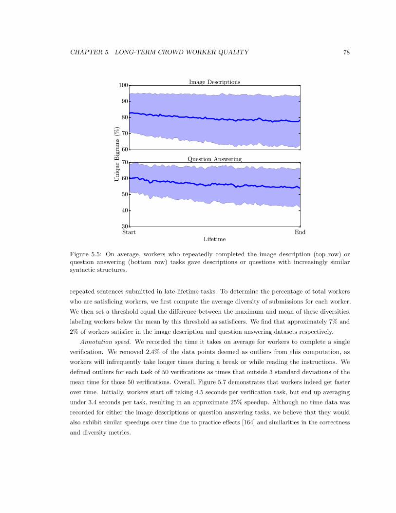
CHAPTER 5. LONG-TERM CROWD WORKER QUALITY 78
60
70
80
90
100 Image Descriptions
Start EndLifetime
30
40
50
60
70
Uniq
ue
Big
ram
s (%
)
Question Answering
Figure 5.5: On average, workers who repeatedly completed the image description (top row) orquestion answering (bottom row) tasks gave descriptions or questions with increasingly similarsyntactic structures.
repeated sentences submitted in late-lifetime tasks. To determine the percentage of total workers
who are satisficing workers, we first compute the average diversity of submissions for each worker.
We then set a threshold equal the difference between the maximum and mean of these diversities,
labeling workers below the mean by this threshold as satisficers. We find that approximately 7% and
2% of workers satisfice in the image description and question answering datasets respectively.
Annotation speed. We recorded the time it takes on average for workers to complete a single
verification. We removed 2.4% of the data points deemed as outliers from this computation, as
workers will infrequently take longer times during a break or while reading the instructions. We
defined outliers for each task of 50 verifications as times that outside 3 standard deviations of the
mean time for those 50 verifications. Overall, Figure 5.7 demonstrates that workers indeed get faster
over time. Initially, workers start off taking 4.5 seconds per verification task, but end up averaging
under 3.4 seconds per task, resulting in an approximate 25% speedup. Although no time data was
recorded for either the image descriptions or question answering tasks, we believe that they would
also exhibit similar speedups over time due to practice effects [164] and similarities in the correctness
and diversity metrics.
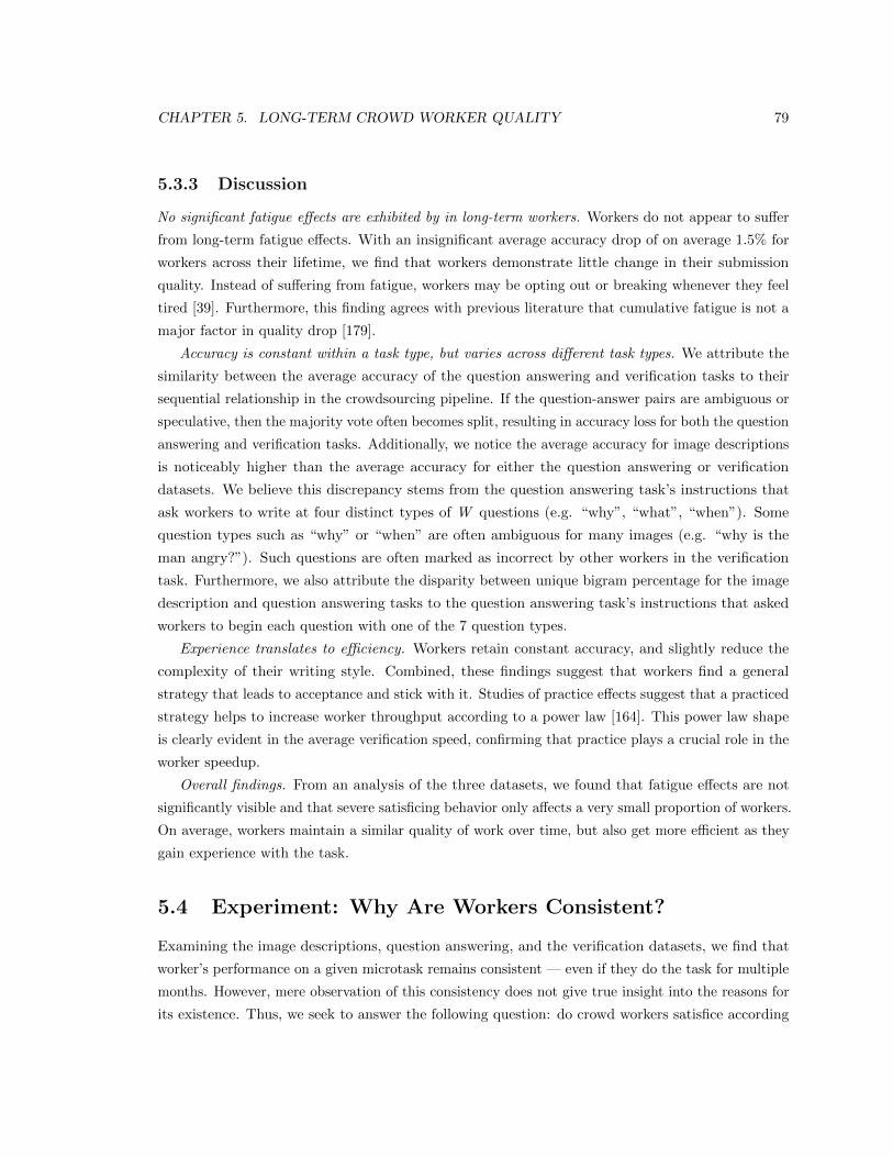
CHAPTER 5. LONG-TERM CROWD WORKER QUALITY 79
5.3.3 Discussion
No significant fatigue effects are exhibited by in long-term workers. Workers do not appear to suffer
from long-term fatigue effects. With an insignificant average accuracy drop of on average 1.5% for
workers across their lifetime, we find that workers demonstrate little change in their submission
quality. Instead of suffering from fatigue, workers may be opting out or breaking whenever they feel
tired [39]. Furthermore, this finding agrees with previous literature that cumulative fatigue is not a
major factor in quality drop [179].
Accuracy is constant within a task type, but varies across different task types. We attribute the
similarity between the average accuracy of the question answering and verification tasks to their
sequential relationship in the crowdsourcing pipeline. If the question-answer pairs are ambiguous or
speculative, then the majority vote often becomes split, resulting in accuracy loss for both the question
answering and verification tasks. Additionally, we notice the average accuracy for image descriptions
is noticeably higher than the average accuracy for either the question answering or verification
datasets. We believe this discrepancy stems from the question answering task’s instructions that
ask workers to write at four distinct types of W questions (e.g. “why”, “what”, “when”). Some
question types such as “why” or “when” are often ambiguous for many images (e.g. “why is the
man angry?”). Such questions are often marked as incorrect by other workers in the verification
task. Furthermore, we also attribute the disparity between unique bigram percentage for the image
description and question answering tasks to the question answering task’s instructions that asked
workers to begin each question with one of the 7 question types.
Experience translates to efficiency. Workers retain constant accuracy, and slightly reduce the
complexity of their writing style. Combined, these findings suggest that workers find a general
strategy that leads to acceptance and stick with it. Studies of practice effects suggest that a practiced
strategy helps to increase worker throughput according to a power law [164]. This power law shape
is clearly evident in the average verification speed, confirming that practice plays a crucial role in the
worker speedup.
Overall findings. From an analysis of the three datasets, we found that fatigue effects are not
significantly visible and that severe satisficing behavior only affects a very small proportion of workers.
On average, workers maintain a similar quality of work over time, but also get more efficient as they
gain experience with the task.
5.4 Experiment: Why Are Workers Consistent?
Examining the image descriptions, question answering, and the verification datasets, we find that
worker’s performance on a given microtask remains consistent — even if they do the task for multiple
months. However, mere observation of this consistency does not give true insight into the reasons for
its existence. Thus, we seek to answer the following question: do crowd workers satisfice according
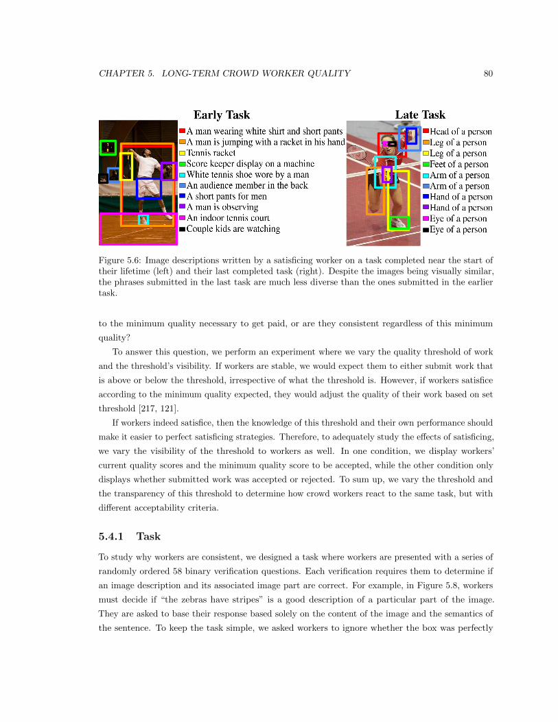
CHAPTER 5. LONG-TERM CROWD WORKER QUALITY 80
Figure 5.6: Image descriptions written by a satisficing worker on a task completed near the start oftheir lifetime (left) and their last completed task (right). Despite the images being visually similar,the phrases submitted in the last task are much less diverse than the ones submitted in the earliertask.
to the minimum quality necessary to get paid, or are they consistent regardless of this minimum
quality?
To answer this question, we perform an experiment where we vary the quality threshold of work
and the threshold’s visibility. If workers are stable, we would expect them to either submit work that
is above or below the threshold, irrespective of what the threshold is. However, if workers satisfice
according to the minimum quality expected, they would adjust the quality of their work based on set
threshold [217, 121].
If workers indeed satisfice, then the knowledge of this threshold and their own performance should
make it easier to perfect satisficing strategies. Therefore, to adequately study the effects of satisficing,
we vary the visibility of the threshold to workers as well. In one condition, we display workers’
current quality scores and the minimum quality score to be accepted, while the other condition only
displays whether submitted work was accepted or rejected. To sum up, we vary the threshold and
the transparency of this threshold to determine how crowd workers react to the same task, but with
different acceptability criteria.
5.4.1 Task
To study why workers are consistent, we designed a task where workers are presented with a series of
randomly ordered 58 binary verification questions. Each verification requires them to determine if
an image description and its associated image part are correct. For example, in Figure 5.8, workers
must decide if “the zebras have stripes” is a good description of a particular part of the image.
They are asked to base their response based solely on the content of the image and the semantics of
the sentence. To keep the task simple, we asked workers to ignore whether the box was perfectly
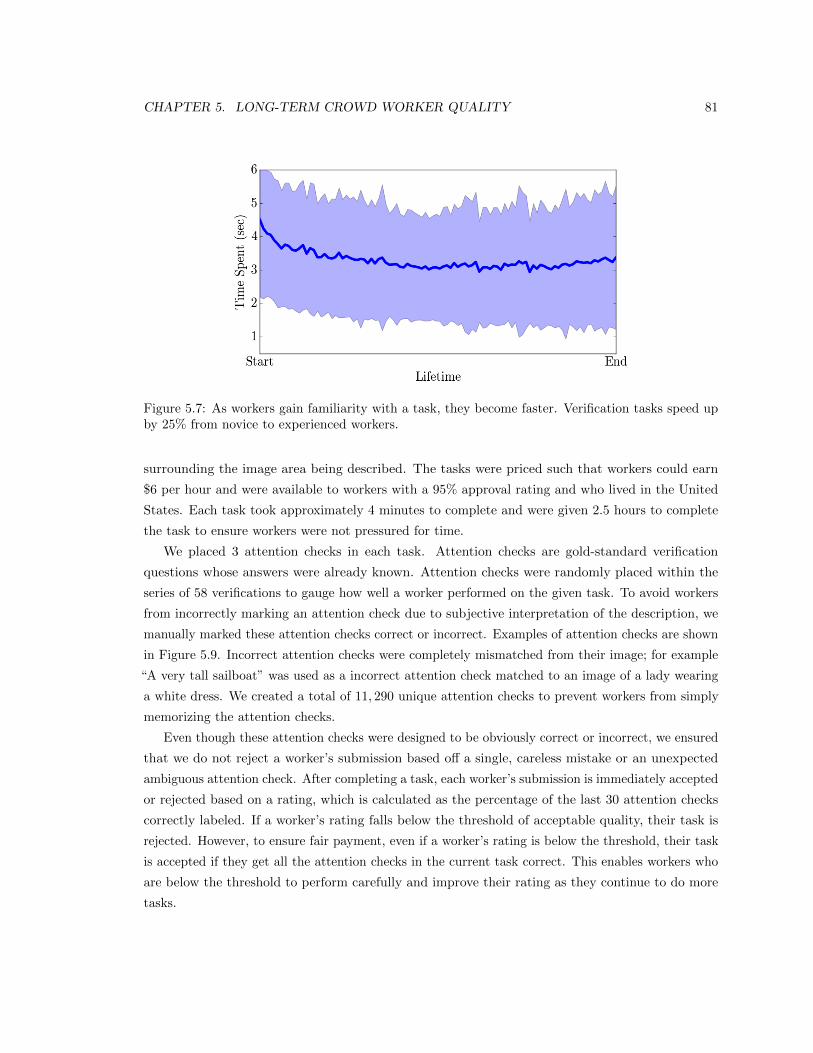
CHAPTER 5. LONG-TERM CROWD WORKER QUALITY 81
Figure 5.7: As workers gain familiarity with a task, they become faster. Verification tasks speed upby 25% from novice to experienced workers.
surrounding the image area being described. The tasks were priced such that workers could earn
$6 per hour and were available to workers with a 95% approval rating and who lived in the United
States. Each task took approximately 4 minutes to complete and were given 2.5 hours to complete
the task to ensure workers were not pressured for time.
We placed 3 attention checks in each task. Attention checks are gold-standard verification
questions whose answers were already known. Attention checks were randomly placed within the
series of 58 verifications to gauge how well a worker performed on the given task. To avoid workers
from incorrectly marking an attention check due to subjective interpretation of the description, we
manually marked these attention checks correct or incorrect. Examples of attention checks are shown
in Figure 5.9. Incorrect attention checks were completely mismatched from their image; for example
“A very tall sailboat” was used as a incorrect attention check matched to an image of a lady wearing
a white dress. We created a total of 11, 290 unique attention checks to prevent workers from simply
memorizing the attention checks.
Even though these attention checks were designed to be obviously correct or incorrect, we ensured
that we do not reject a worker’s submission based off a single, careless mistake or an unexpected
ambiguous attention check. After completing a task, each worker’s submission is immediately accepted
or rejected based on a rating, which is calculated as the percentage of the last 30 attention checks
correctly labeled. If a worker’s rating falls below the threshold of acceptable quality, their task is
rejected. However, to ensure fair payment, even if a worker’s rating is below the threshold, their task
is accepted if they get all the attention checks in the current task correct. This enables workers who
are below the threshold to perform carefully and improve their rating as they continue to do more
tasks.
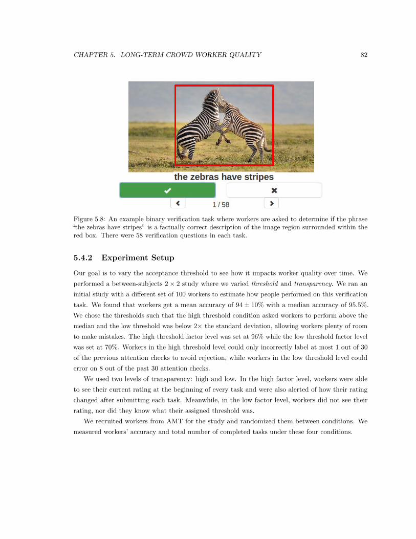
CHAPTER 5. LONG-TERM CROWD WORKER QUALITY 82
Figure 5.8: An example binary verification task where workers are asked to determine if the phrase“the zebras have stripes” is a factually correct description of the image region surrounded within thered box. There were 58 verification questions in each task.
5.4.2 Experiment Setup
Our goal is to vary the acceptance threshold to see how it impacts worker quality over time. We
performed a between-subjects 2× 2 study where we varied threshold and transparency. We ran an
initial study with a different set of 100 workers to estimate how people performed on this verification
task. We found that workers get a mean accuracy of 94 ± 10% with a median accuracy of 95.5%.
We chose the thresholds such that the high threshold condition asked workers to perform above the
median and the low threshold was below 2× the standard deviation, allowing workers plenty of room
to make mistakes. The high threshold factor level was set at 96% while the low threshold factor level
was set at 70%. Workers in the high threshold level could only incorrectly label at most 1 out of 30
of the previous attention checks to avoid rejection, while workers in the low threshold level could
error on 8 out of the past 30 attention checks.
We used two levels of transparency: high and low. In the high factor level, workers were able
to see their current rating at the beginning of every task and were also alerted of how their rating
changed after submitting each task. Meanwhile, in the low factor level, workers did not see their
rating, nor did they know what their assigned threshold was.
We recruited workers from AMT for the study and randomized them between conditions. We
measured workers’ accuracy and total number of completed tasks under these four conditions.
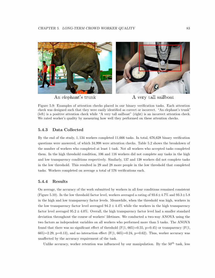
CHAPTER 5. LONG-TERM CROWD WORKER QUALITY 83
Figure 5.9: Examples of attention checks placed in our binary verification tasks. Each attentioncheck was designed such that they were easily identified as correct or incorrect. “An elephant’s trunk”(left) is a positive attention check while “A very tall sailboat” (right) is an incorrect attention check.We rated worker’s quality by measuring how well they performed on these attention checks.
5.4.3 Data Collected
By the end of the study, 1, 134 workers completed 11,666 tasks. In total, 676,628 binary verification
questions were answered, of which 34,998 were attention checks. Table 5.2 shows the breakdown of
the number of workers who completed at least 1 task. Not all workers who accepted tasks completed
them. In the high threshold condition, 106 and 116 workers did not complete any tasks in the high
and low transparency conditions respectively. Similarly, 137 and 138 workers did not complete tasks
in the low threshold. This resulted in 29 and 28 more people in the low threshold that completed
tasks. Workers completed on average a total of 576 verifications each.
5.4.4 Results
On average, the accuracy of the work submitted by workers in all four conditions remained consistent
(Figure 5.10). In the low threshold factor level, workers averaged a rating of 93.6±4.7% and 93.3±5.8
in the high and low transparency factor levels. Meanwhile, when the threshold was high, workers in
the low transparency factor level averaged 94.2± 4.4% while the workers in the high transparency
factor level averaged 95.2± 4.0%. Overall, the high transparency factor level had a smaller standard
deviation throughout the course of workers’ lifetimes. We conducted a two-way ANOVA using the
two factors as independent variables on all workers who performed more than 5 tasks. The ANOVA
found that there was no significant effect of threshold (F(1, 665)=0.55, p=0.45) or transparency (F(1,
665)=2.29, p=0.13), and no interaction effect (F(1, 665)=0.24, p=0.62). Thus, worker accuracy was
unaffected by the accuracy requirement of the task.
Unlike accuracy, worker retention was influenced by our manipulation. By the 50th task, less
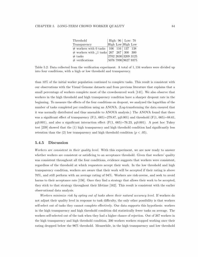
CHAPTER 5. LONG-TERM CROWD WORKER QUALITY 84
Threshold High: 96 Low: 70Transparency High Low High Low
# workers with 0 tasks 106 116 137 138# workers with ¿1 tasks 267 267 300 300# tasks 2702 2630 3209 3125# verifications 5076 7890 9627 9375
Table 5.2: Data collected from the verification experiment. A total of 1, 134 workers were divided upinto four conditions, with a high or low threshold and transparency.
than 10% of the initial worker population continued to complete tasks. This result is consistent with
our observations with the Visual Genome datasets and from previous literature that explains that a
small percentage of workers complete most of the crowdsourced work [141]. We also observe that
workers in the high threshold and high transparency condition have a sharper dropout rate in the
beginning. To measure the effects of the four conditions on dropout, we analyzed the logarithm of the
number of tasks completed per condition using an ANOVA. (Log-transforming the data ensured that
it was normally distributed and thus amenable to ANOVA analysis.) The ANOVA found that there
was a significant effect of transparency (F(1, 665)=279.87, p¡0.001) and threshold (F(1, 665)=88.61,
p¡0.001), and also a significant interaction effect (F(1, 665)=76.23, p¡0.001). A post hoc Tukey
test [239] showed that the (1) high transparency and high threshold condition had significantly less
retention than the (2) low transparency and high threshold condition (p < .05).
5.4.5 Discussion
Workers are consistent in their quality level. With this experiment, we are now ready to answer
whether workers are consistent or satisficing to an acceptance threshold. Given that workers’ quality
was consistent throughout all the four conditions, evidence suggests that workers were consistent,
regardless of the threshold at which requesters accept their work. In the low threshold and high
transparency condition, workers are aware that their work will be accepted if their rating is above
70%, and still perform with an average rating of 94%. Workers are risk-averse, and seek to avoid
harms to their acceptance rate [156]. Once they find a strategy that allows their work to be accepted,
they stick to that strategy throughout their lifetime [162]. This result is consistent with the earlier
observational data analysis.
Workers minimize risk by opting out of tasks above their natural accuracy level. If workers do
not adjust their quality level in response to task difficulty, the only other possibility is that workers
self-select out of tasks they cannot complete effectively. Our data supports this hypothesis: workers
in the high transparency and high threshold condition did statistically fewer tasks on average. The
workers self-selected out of the task when they had a higher chance of rejection. Out of 267 workers in
the high transparency and high threshold condition, 200 workers workers stopped working once their
rating dropped below the 96% threshold. Meanwhile, in the high transparency and low threshold
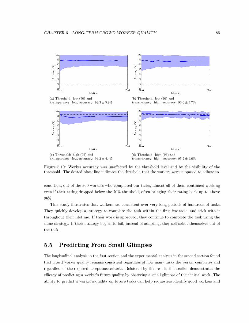
CHAPTER 5. LONG-TERM CROWD WORKER QUALITY 85
(a) Threshold: low (70) andtransparency: low, accuracy: 93.3 ± 5.8%
(b) Threshold: low (70) andtransparency: high, accuracy: 93.6 ± 4.7%
(c) Threshold: high (96) andtransparency: low, accuracy: 94.2 ± 4.4%
(d) Threshold: high (96) andtransparency: high, accuracy: 95.2 ± 4.0%
Figure 5.10: Worker accuracy was unaffected by the threshold level and by the visibility of thethreshold. The dotted black line indicates the threshold that the workers were supposed to adhere to.
condition, out of the 300 workers who completed our tasks, almost all of them continued working
even if their rating dropped below the 70% threshold, often bringing their rating back up to above
96%.
This study illustrates that workers are consistent over very long periods of hundreds of tasks.
They quickly develop a strategy to complete the task within the first few tasks and stick with it
throughout their lifetime. If their work is approved, they continue to complete the task using the
same strategy. If their strategy begins to fail, instead of adapting, they self-select themselves out of
the task.
5.5 Predicting From Small Glimpses
The longitudinal analysis in the first section and the experimental analysis in the second section found
that crowd worker quality remains consistent regardless of how many tasks the worker completes and
regardless of the required acceptance criteria. Bolstered by this result, this section demonstrates the
efficacy of predicting a worker’s future quality by observing a small glimpse of their initial work. The
ability to predict a worker’s quality on future tasks can help requesters identify good workers and
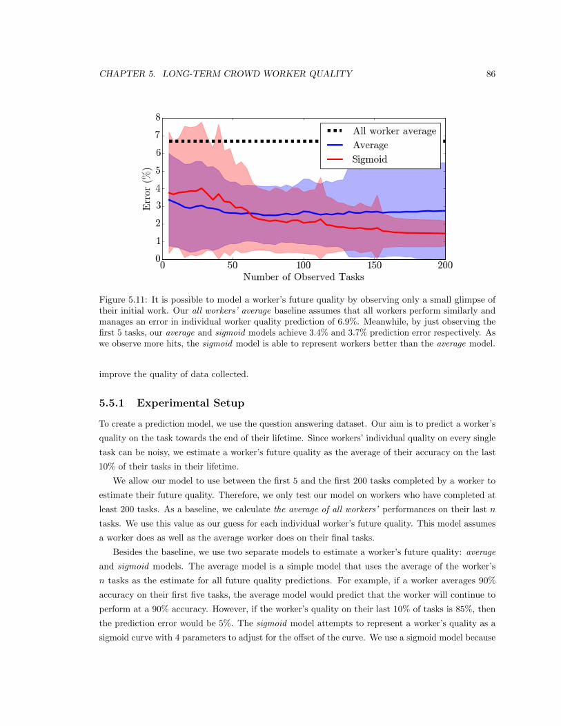
CHAPTER 5. LONG-TERM CROWD WORKER QUALITY 86
Figure 5.11: It is possible to model a worker’s future quality by observing only a small glimpse oftheir initial work. Our all workers’ average baseline assumes that all workers perform similarly andmanages an error in individual worker quality prediction of 6.9%. Meanwhile, by just observing thefirst 5 tasks, our average and sigmoid models achieve 3.4% and 3.7% prediction error respectively. Aswe observe more hits, the sigmoid model is able to represent workers better than the average model.
improve the quality of data collected.
5.5.1 Experimental Setup
To create a prediction model, we use the question answering dataset. Our aim is to predict a worker’s
quality on the task towards the end of their lifetime. Since workers’ individual quality on every single
task can be noisy, we estimate a worker’s future quality as the average of their accuracy on the last
10% of their tasks in their lifetime.
We allow our model to use between the first 5 and the first 200 tasks completed by a worker to
estimate their future quality. Therefore, we only test our model on workers who have completed at
least 200 tasks. As a baseline, we calculate the average of all workers’ performances on their last n
tasks. We use this value as our guess for each individual worker’s future quality. This model assumes
a worker does as well as the average worker does on their final tasks.
Besides the baseline, we use two separate models to estimate a worker’s future quality: average
and sigmoid models. The average model is a simple model that uses the average of the worker’s
n tasks as the estimate for all future quality predictions. For example, if a worker averages 90%
accuracy on their first five tasks, the average model would predict that the worker will continue to
perform at a 90% accuracy. However, if the worker’s quality on their last 10% of tasks is 85%, then
the prediction error would be 5%. The sigmoid model attempts to represent a worker’s quality as a
sigmoid curve with 4 parameters to adjust for the offset of the curve. We use a sigmoid model because
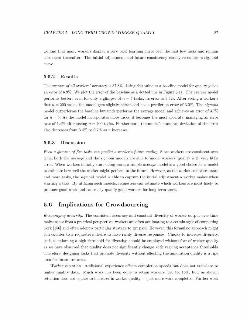
CHAPTER 5. LONG-TERM CROWD WORKER QUALITY 87
we find that many workers display a very brief learning curve over the first few tasks and remain
consistent thereafter. The initial adjustment and future consistency closely resembles a sigmoid
curve.
5.5.2 Results
The average of all workers’ accuracy is 87.8%. Using this value as a baseline model for quality yields
an error of 6.9%. We plot the error of the baseline as a dotted line in Figure 5.11. The average model
performs better: even for only a glimpse of n = 5 tasks, its error is 3.4%. After seeing a worker’s
first n = 200 tasks, the model gets slightly better and has a prediction error of 3.0%. The sigmoid
model outperforms the baseline but underperforms the average model and achieves an error of 3.7%
for n = 5. As the model incorporates more tasks, it becomes the most accurate, managing an error
rate of 1.4% after seeing n = 200 tasks. Furthermore, the model’s standard deviation of the error
also decreases from 3.4% to 0.7% as n increases.
5.5.3 Discussion
Even a glimpse of five tasks can predict a worker’s future quality. Since workers are consistent over
time, both the average and the sigmoid models are able to model workers’ quality with very little
error. When workers initially start doing work, a simple average model is a good choice for a model
to estimate how well the worker might perform in the future. However, as the worker completes more
and more tasks, the sigmoid model is able to capture the initial adjustment a worker makes when
starting a task. By utilizing such models, requesters can estimate which workers are most likely to
produce good work and can easily qualify good workers for long-term work.
5.6 Implications for Crowdsourcing
Encouraging diversity. The consistent accuracy and constant diversity of worker output over time
makes sense from a practical perspective: workers are often acclimating to a certain style of completing
work [156] and often adopt a particular strategy to get paid. However, this formulaic approach might
run counter to a requester’s desire to have richly diverse responses. Checks to increase diversity,
such as enforcing a high threshold for diversity, should be employed without fear of worker quality
as we have observed that quality does not significantly change with varying acceptance thresholds.
Therefore, designing tasks that promote diversity without effecting the annotation quality is a ripe
area for future research.
Worker retention. Additional experience affects completion speeds but does not translate to
higher quality data. Much work has been done to retain workers [39, 46, 133], but, as shown,
retention does not equate to increases in worker quality — just more work completed. Further work
CHAPTER 5. LONG-TERM CROWD WORKER QUALITY 88
should be conducted to not only retain a worker pool, but also examine methods of identifying good
workers [107] and more direct interventions for training poorly performing workers [50, 112].
Additionally, other studies have shown that the motivation of workers is the predominant factor
in the development of fatigue, rather than the total time worked [6]. Although crowdsourcing can be
intrinsically motivated [248], the microtask paradigm found in the majority of crowdsourcing tasks
favors a structure that is efficient [119, 85] for workers rather than being interesting for them [26].
Future tasks should consider building continuity in their workflow design for both individual worker
efficiency [130] and overall throughput and retention [39].
Person-centric versus process-centric crowdsourcing. Attaining high quality judgments from crowd
workers is often seen as a challenge [186, 213, 227]. This challenge has catalyzed studies suggesting
quality control measures that address the problem of noisy or low quality work [51, 112, 155]. Many
of these investigations study various quality-control measures as standalone intervention strategies.
While we explored process-centric measures like varying the acceptance or transparency threshold,
previous work has experimented with varying financial incentives [162]. All the results support the
conclusion that process-centric strategies do not have significant difference in the quality of work
submitted. While we agree that such process focused strategies are important to explore, our data
reinforces that person-centric strategies (like utilizing worker approval ratings or worker quality on
initial tasks) may be more effective [162, 202] because they identify a worker’s (consistent) quality
early on.
Limitations. Our analysis solely focuses on data labeling microtasks, and we have not yet studied
whether our findings translate over to more complex tasks, such as designing an advertisement or
editing an essay [114, 8]. Furthermore, we focus on weeks-to-months crowd worker behavior based
on datasets collected over a few months, but there exist some crowdsourcing tasks [17] that have
persisted far longer than our study. Thus, we leave the analysis of crowd worker behavior spanning
multiple years to future work.
5.7 Conclusion
Microtask crowdsourcing is rapidly being adopted to generate large datasets with millions of labels.
Under the Pareto principle, a small minority of workers complete a great majority of the work. In
this paper, we studied how the quality of workers’ submissions change over extended periods of time
as they complete thousands of tasks. Contrary to previous literature on fatigue and satisficing, we
found that workers are extremely consistent throughout their lifetime of submitting work. They
adopt a particular strategy for completing tasks and continue to use that strategy without change. To
understand how workers settle upon their strategy, we conducted an experiment where we vary the
required quality for large crowdsourcing tasks. We found that workers do not satisfice and consistently
perform at their usual quality level. If their natural quality level is below the acceptance threshold,

CHAPTER 5. LONG-TERM CROWD WORKER QUALITY 89
workers tend to opt out from completing further tasks. Due to this consistency, we demonstrated
that brief glimpses of just the first five tasks can predict a worker’s long-term quality. We argue that
such consistent worker behavior must be utilized to develop new crowdsourcing strategies that find
good workers and collect unvarying high quality annotations.
Chapter 6
Leveraging Representations in
Visual Genome
6.1 Introduction
Thus far, we have presented the Visual Genome dataset, improved its crowdsourcing pipeline, and
analyzed the types of annotations included. With such rich information provided, numerous perceptual
and cognitive tasks can be tackled. In this section, we aim to provide baseline experimental results
using components of Visual Genome that have not been extensively studied. Object detection is
already a well-studied problem [54, 71, 212, 70, 190]. Similarly, region graphs and scene graphs have
been shown to improve semantic image retrieval [102, 210]. We therefore focus on the remaining
components, i.e. attributes, relationships, region descriptions, and question answer pairs.
In Section 6.1.1, we present results for two experiments on attribute prediction. In the first, we
treat attributes independently from objects and train a classifier for each attribute, i.e. a classifier for
red or a classifier for old, as in [148, 241, 61, 57, 102]. In the second experiment, we learn object
and attribute classifiers jointly and predict object-attribute pairs (e.g. predicting that an apple is
red), as in [204].
In Section 6.1.2, we present two experiments on relationship prediction. In the first, we aim
to predict the predicate between two objects, e.g. predicting the predicate kicking or wearing
between two objects. This experiment is synonymous with existing work in action recognition [79, 185].
In another experiment, we study relationships by classifying jointly the objects and the predicate (e.g.
predicting kicking(man, ball)); we show that this is a very difficult task due to the high variability in
the appearance of a relationship (e.g. the ball might be on the ground or in mid-air above the man).
These experiments are generalizations of tasks that study spatial relationships between objects and
ones that jointly reason about the interaction of humans with objects [270, 184].
90
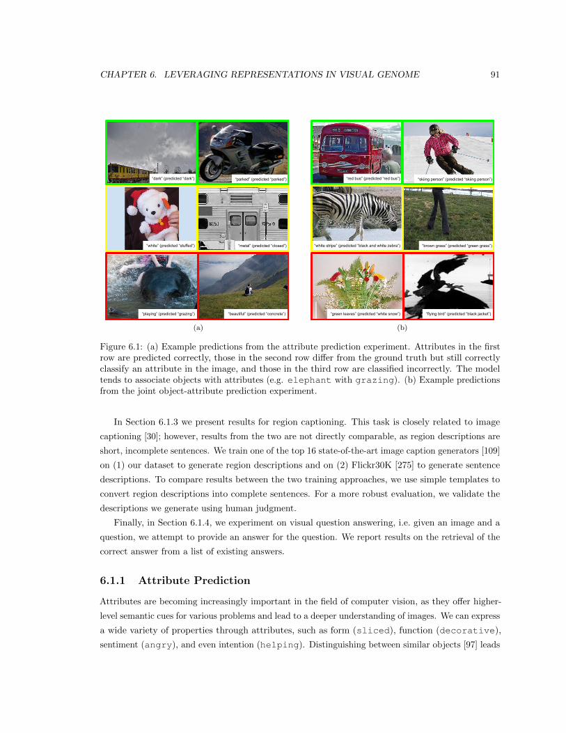
CHAPTER 6. LEVERAGING REPRESENTATIONS IN VISUAL GENOME 91
“playing” (predicted “grazing”) “beautiful” (predicted “concrete”)
“metal” (predicted “closed”)
“dark” (predicted “dark”) “parked” (predicted “parked”)
“white” (predicted “stuffed”)
(a)
“green leaves” (predicted “white snow”) “flying bird” (predicted “black jacket”)
“brown grass” (predicted “green grass”)
“red bus” (predicted “red bus”) “skiing person” (predicted “skiing person”)
“white stripe” (predicted “black and white zebra”)
(b)
Figure 6.1: (a) Example predictions from the attribute prediction experiment. Attributes in the firstrow are predicted correctly, those in the second row differ from the ground truth but still correctlyclassify an attribute in the image, and those in the third row are classified incorrectly. The modeltends to associate objects with attributes (e.g. elephant with grazing). (b) Example predictionsfrom the joint object-attribute prediction experiment.
In Section 6.1.3 we present results for region captioning. This task is closely related to image
captioning [30]; however, results from the two are not directly comparable, as region descriptions are
short, incomplete sentences. We train one of the top 16 state-of-the-art image caption generators [109]
on (1) our dataset to generate region descriptions and on (2) Flickr30K [275] to generate sentence
descriptions. To compare results between the two training approaches, we use simple templates to
convert region descriptions into complete sentences. For a more robust evaluation, we validate the
descriptions we generate using human judgment.
Finally, in Section 6.1.4, we experiment on visual question answering, i.e. given an image and a
question, we attempt to provide an answer for the question. We report results on the retrieval of the
correct answer from a list of existing answers.
6.1.1 Attribute Prediction
Attributes are becoming increasingly important in the field of computer vision, as they offer higher-
level semantic cues for various problems and lead to a deeper understanding of images. We can express
a wide variety of properties through attributes, such as form (sliced), function (decorative),
sentiment (angry), and even intention (helping). Distinguishing between similar objects [97] leads
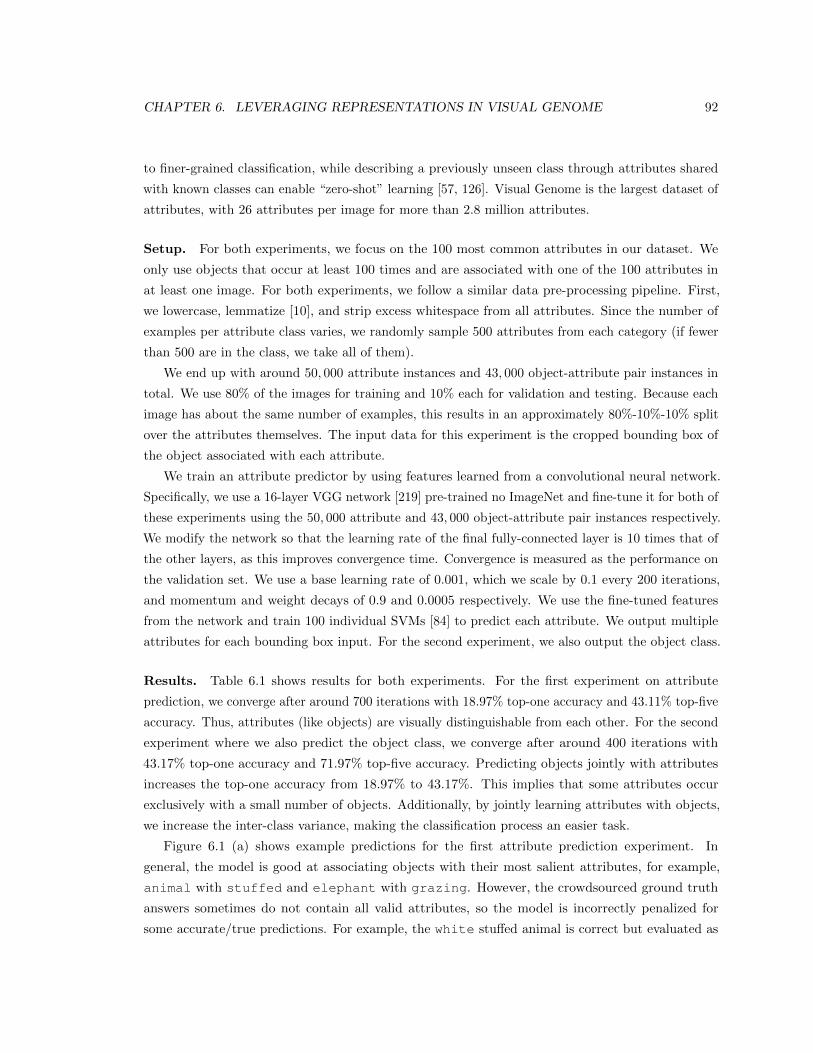
CHAPTER 6. LEVERAGING REPRESENTATIONS IN VISUAL GENOME 92
to finer-grained classification, while describing a previously unseen class through attributes shared
with known classes can enable “zero-shot” learning [57, 126]. Visual Genome is the largest dataset of
attributes, with 26 attributes per image for more than 2.8 million attributes.
Setup. For both experiments, we focus on the 100 most common attributes in our dataset. We
only use objects that occur at least 100 times and are associated with one of the 100 attributes in
at least one image. For both experiments, we follow a similar data pre-processing pipeline. First,
we lowercase, lemmatize [10], and strip excess whitespace from all attributes. Since the number of
examples per attribute class varies, we randomly sample 500 attributes from each category (if fewer
than 500 are in the class, we take all of them).
We end up with around 50, 000 attribute instances and 43, 000 object-attribute pair instances in
total. We use 80% of the images for training and 10% each for validation and testing. Because each
image has about the same number of examples, this results in an approximately 80%-10%-10% split
over the attributes themselves. The input data for this experiment is the cropped bounding box of
the object associated with each attribute.
We train an attribute predictor by using features learned from a convolutional neural network.
Specifically, we use a 16-layer VGG network [219] pre-trained no ImageNet and fine-tune it for both of
these experiments using the 50, 000 attribute and 43, 000 object-attribute pair instances respectively.
We modify the network so that the learning rate of the final fully-connected layer is 10 times that of
the other layers, as this improves convergence time. Convergence is measured as the performance on
the validation set. We use a base learning rate of 0.001, which we scale by 0.1 every 200 iterations,
and momentum and weight decays of 0.9 and 0.0005 respectively. We use the fine-tuned features
from the network and train 100 individual SVMs [84] to predict each attribute. We output multiple
attributes for each bounding box input. For the second experiment, we also output the object class.
Results. Table 6.1 shows results for both experiments. For the first experiment on attribute
prediction, we converge after around 700 iterations with 18.97% top-one accuracy and 43.11% top-five
accuracy. Thus, attributes (like objects) are visually distinguishable from each other. For the second
experiment where we also predict the object class, we converge after around 400 iterations with
43.17% top-one accuracy and 71.97% top-five accuracy. Predicting objects jointly with attributes
increases the top-one accuracy from 18.97% to 43.17%. This implies that some attributes occur
exclusively with a small number of objects. Additionally, by jointly learning attributes with objects,
we increase the inter-class variance, making the classification process an easier task.
Figure 6.1 (a) shows example predictions for the first attribute prediction experiment. In
general, the model is good at associating objects with their most salient attributes, for example,
animal with stuffed and elephant with grazing. However, the crowdsourced ground truth
answers sometimes do not contain all valid attributes, so the model is incorrectly penalized for
some accurate/true predictions. For example, the white stuffed animal is correct but evaluated as
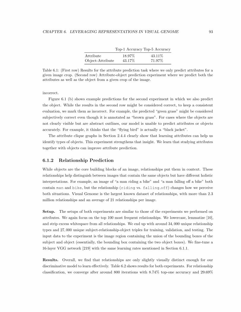
CHAPTER 6. LEVERAGING REPRESENTATIONS IN VISUAL GENOME 93
Top-1 Accuracy Top-5 Accuracy
Attribute 18.97% 43.11%Object-Attribute 43.17% 71.97%
Table 6.1: (First row) Results for the attribute prediction task where we only predict attributes for agiven image crop. (Second row) Attribute-object prediction experiment where we predict both theattributes as well as the object from a given crop of the image.
incorrect.
Figure 6.1 (b) shows example predictions for the second experiment in which we also predict
the object. While the results in the second row might be considered correct, to keep a consistent
evaluation, we mark them as incorrect. For example, the predicted “green grass” might be considered
subjectively correct even though it is annotated as “brown grass”. For cases where the objects are
not clearly visible but are abstract outlines, our model is unable to predict attributes or objects
accurately. For example, it thinks that the “flying bird” is actually a “black jacket”.
The attribute clique graphs in Section 2.4.4 clearly show that learning attributes can help us
identify types of objects. This experiment strengthens that insight. We learn that studying attributes
together with objects can improve attribute prediction.
6.1.2 Relationship Prediction
While objects are the core building blocks of an image, relationships put them in context. These
relationships help distinguish between images that contain the same objects but have different holistic
interpretations. For example, an image of “a man riding a bike” and “a man falling off a bike” both
contain man and bike, but the relationship (riding vs. falling off) changes how we perceive
both situations. Visual Genome is the largest known dataset of relationships, with more than 2.3
million relationships and an average of 21 relationships per image.
Setup. The setups of both experiments are similar to those of the experiments we performed on
attributes. We again focus on the top 100 most frequent relationships. We lowercase, lemmatize [10],
and strip excess whitespace from all relationships. We end up with around 34, 000 unique relationship
types and 27, 000 unique subject-relationship-object triples for training, validation, and testing. The
input data to the experiment is the image region containing the union of the bounding boxes of the
subject and object (essentially, the bounding box containing the two object boxes). We fine-tune a
16-layer VGG network [219] with the same learning rates mentioned in Section 6.1.1.
Results. Overall, we find that relationships are only slightly visually distinct enough for our
discriminative model to learn effectively. Table 6.2 shows results for both experiments. For relationship
classification, we converge after around 800 iterations with 8.74% top-one accuracy and 29.69%
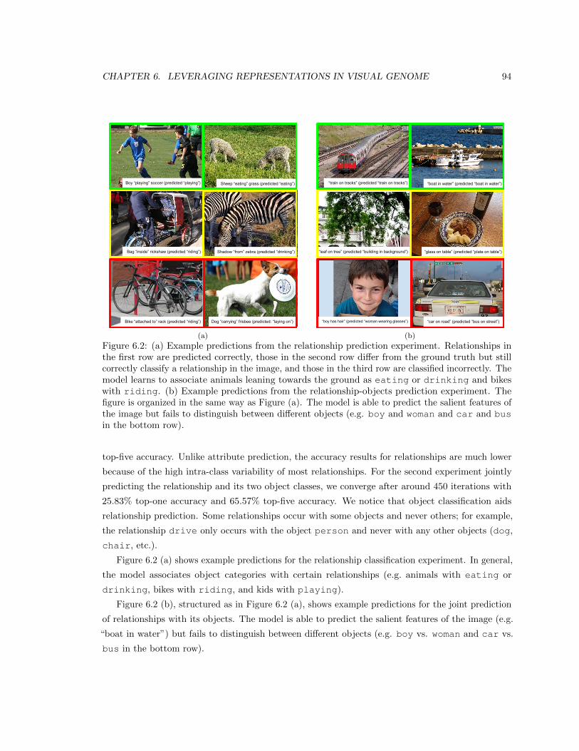
CHAPTER 6. LEVERAGING REPRESENTATIONS IN VISUAL GENOME 94
Dog “carrying” frisbee (predicted: “laying on”)
Boy “playing” soccer (predicted “playing”) Sheep “eating” grass (predicted “eating”)
Bike “attached to” rack (predicted “riding”)
Bag “inside” rickshaw (predicted “riding”) Shadow “from” zebra (predicted “drinking”)
(a)
“glass on table” (predicted “plate on table”)
“car on road” (predicted “bus on street”)
“train on tracks” (predicted “train on tracks”)
“leaf on tree” (predicted “building in background”)
“boat in water” (predicted “boat in water”)
“boy has hair” (predicted “woman wearing glasses”)
(b)
Figure 6.2: (a) Example predictions from the relationship prediction experiment. Relationships inthe first row are predicted correctly, those in the second row differ from the ground truth but stillcorrectly classify a relationship in the image, and those in the third row are classified incorrectly. Themodel learns to associate animals leaning towards the ground as eating or drinking and bikeswith riding. (b) Example predictions from the relationship-objects prediction experiment. Thefigure is organized in the same way as Figure (a). The model is able to predict the salient features ofthe image but fails to distinguish between different objects (e.g. boy and woman and car and busin the bottom row).
top-five accuracy. Unlike attribute prediction, the accuracy results for relationships are much lower
because of the high intra-class variability of most relationships. For the second experiment jointly
predicting the relationship and its two object classes, we converge after around 450 iterations with
25.83% top-one accuracy and 65.57% top-five accuracy. We notice that object classification aids
relationship prediction. Some relationships occur with some objects and never others; for example,
the relationship drive only occurs with the object person and never with any other objects (dog,
chair, etc.).
Figure 6.2 (a) shows example predictions for the relationship classification experiment. In general,
the model associates object categories with certain relationships (e.g. animals with eating or
drinking, bikes with riding, and kids with playing).
Figure 6.2 (b), structured as in Figure 6.2 (a), shows example predictions for the joint prediction
of relationships with its objects. The model is able to predict the salient features of the image (e.g.
“boat in water”) but fails to distinguish between different objects (e.g. boy vs. woman and car vs.
bus in the bottom row).
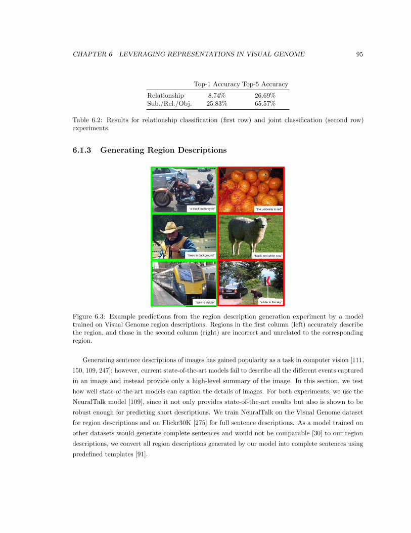
CHAPTER 6. LEVERAGING REPRESENTATIONS IN VISUAL GENOME 95
Top-1 Accuracy Top-5 Accuracy
Relationship 8.74% 26.69%Sub./Rel./Obj. 25.83% 65.57%
Table 6.2: Results for relationship classification (first row) and joint classification (second row)experiments.
6.1.3 Generating Region Descriptions
“a black motorcycle”
“trees in background”
“train is visible”
“the umbrella is red”
“black and white cow”
“a kite in the sky”
Figure 6.3: Example predictions from the region description generation experiment by a modeltrained on Visual Genome region descriptions. Regions in the first column (left) accurately describethe region, and those in the second column (right) are incorrect and unrelated to the correspondingregion.
Generating sentence descriptions of images has gained popularity as a task in computer vision [111,
150, 109, 247]; however, current state-of-the-art models fail to describe all the different events captured
in an image and instead provide only a high-level summary of the image. In this section, we test
how well state-of-the-art models can caption the details of images. For both experiments, we use the
NeuralTalk model [109], since it not only provides state-of-the-art results but also is shown to be
robust enough for predicting short descriptions. We train NeuralTalk on the Visual Genome dataset
for region descriptions and on Flickr30K [275] for full sentence descriptions. As a model trained on
other datasets would generate complete sentences and would not be comparable [30] to our region
descriptions, we convert all region descriptions generated by our model into complete sentences using
predefined templates [91].
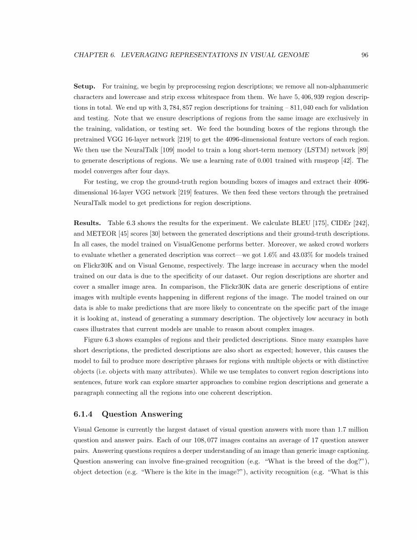
CHAPTER 6. LEVERAGING REPRESENTATIONS IN VISUAL GENOME 96
Setup. For training, we begin by preprocessing region descriptions; we remove all non-alphanumeric
characters and lowercase and strip excess whitespace from them. We have 5, 406, 939 region descrip-
tions in total. We end up with 3, 784, 857 region descriptions for training – 811, 040 each for validation
and testing. Note that we ensure descriptions of regions from the same image are exclusively in
the training, validation, or testing set. We feed the bounding boxes of the regions through the
pretrained VGG 16-layer network [219] to get the 4096-dimensional feature vectors of each region.
We then use the NeuralTalk [109] model to train a long short-term memory (LSTM) network [89]
to generate descriptions of regions. We use a learning rate of 0.001 trained with rmsprop [42]. The
model converges after four days.
For testing, we crop the ground-truth region bounding boxes of images and extract their 4096-
dimensional 16-layer VGG network [219] features. We then feed these vectors through the pretrained
NeuralTalk model to get predictions for region descriptions.
Results. Table 6.3 shows the results for the experiment. We calculate BLEU [175], CIDEr [242],
and METEOR [45] scores [30] between the generated descriptions and their ground-truth descriptions.
In all cases, the model trained on VisualGenome performs better. Moreover, we asked crowd workers
to evaluate whether a generated description was correct—we got 1.6% and 43.03% for models trained
on Flickr30K and on Visual Genome, respectively. The large increase in accuracy when the model
trained on our data is due to the specificity of our dataset. Our region descriptions are shorter and
cover a smaller image area. In comparison, the Flickr30K data are generic descriptions of entire
images with multiple events happening in different regions of the image. The model trained on our
data is able to make predictions that are more likely to concentrate on the specific part of the image
it is looking at, instead of generating a summary description. The objectively low accuracy in both
cases illustrates that current models are unable to reason about complex images.
Figure 6.3 shows examples of regions and their predicted descriptions. Since many examples have
short descriptions, the predicted descriptions are also short as expected; however, this causes the
model to fail to produce more descriptive phrases for regions with multiple objects or with distinctive
objects (i.e. objects with many attributes). While we use templates to convert region descriptions into
sentences, future work can explore smarter approaches to combine region descriptions and generate a
paragraph connecting all the regions into one coherent description.
6.1.4 Question Answering
Visual Genome is currently the largest dataset of visual question answers with more than 1.7 million
question and answer pairs. Each of our 108, 077 images contains an average of 17 question answer
pairs. Answering questions requires a deeper understanding of an image than generic image captioning.
Question answering can involve fine-grained recognition (e.g. “What is the breed of the dog?”),
object detection (e.g. “Where is the kite in the image?”), activity recognition (e.g. “What is this
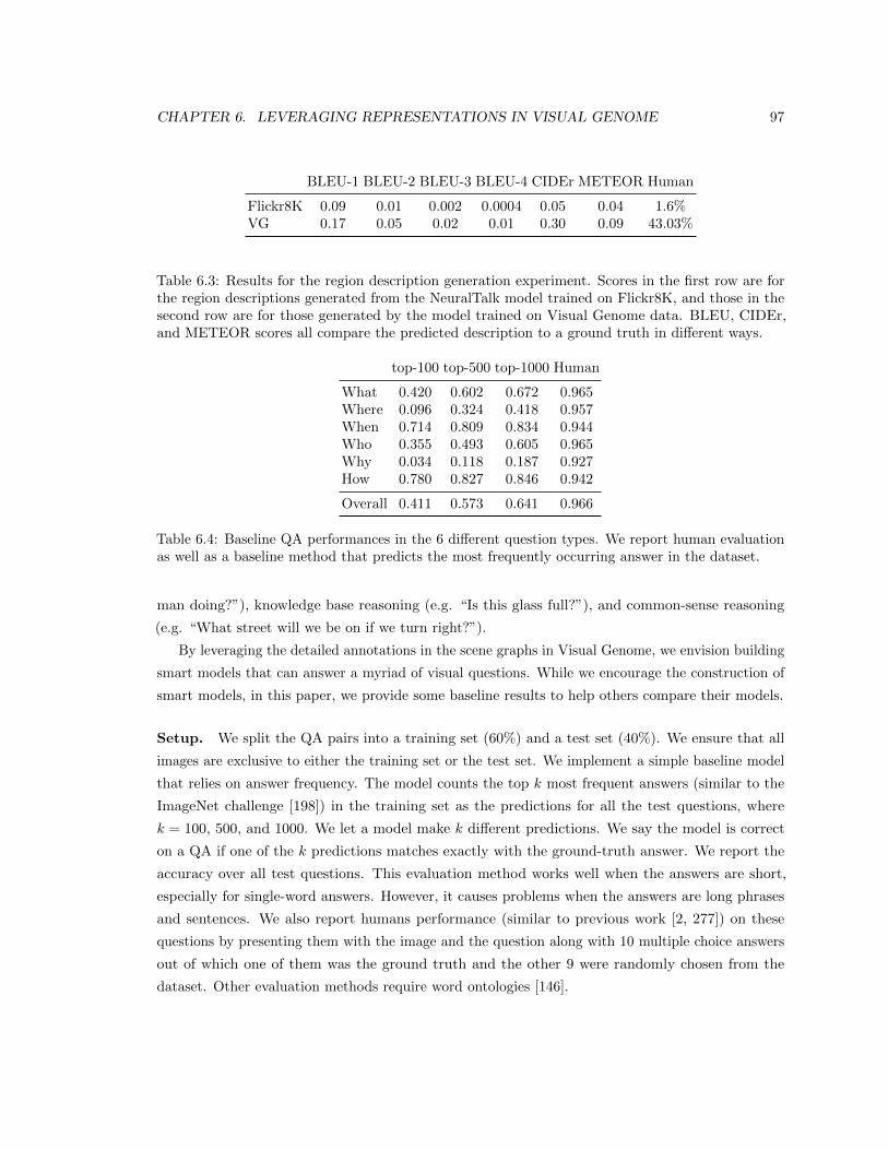
CHAPTER 6. LEVERAGING REPRESENTATIONS IN VISUAL GENOME 97
BLEU-1 BLEU-2 BLEU-3 BLEU-4 CIDEr METEOR Human
Flickr8K 0.09 0.01 0.002 0.0004 0.05 0.04 1.6%VG 0.17 0.05 0.02 0.01 0.30 0.09 43.03%
Table 6.3: Results for the region description generation experiment. Scores in the first row are forthe region descriptions generated from the NeuralTalk model trained on Flickr8K, and those in thesecond row are for those generated by the model trained on Visual Genome data. BLEU, CIDEr,and METEOR scores all compare the predicted description to a ground truth in different ways.
top-100 top-500 top-1000 Human
What 0.420 0.602 0.672 0.965Where 0.096 0.324 0.418 0.957When 0.714 0.809 0.834 0.944Who 0.355 0.493 0.605 0.965Why 0.034 0.118 0.187 0.927How 0.780 0.827 0.846 0.942
Overall 0.411 0.573 0.641 0.966
Table 6.4: Baseline QA performances in the 6 different question types. We report human evaluationas well as a baseline method that predicts the most frequently occurring answer in the dataset.
man doing?”), knowledge base reasoning (e.g. “Is this glass full?”), and common-sense reasoning
(e.g. “What street will we be on if we turn right?”).
By leveraging the detailed annotations in the scene graphs in Visual Genome, we envision building
smart models that can answer a myriad of visual questions. While we encourage the construction of
smart models, in this paper, we provide some baseline results to help others compare their models.
Setup. We split the QA pairs into a training set (60%) and a test set (40%). We ensure that all
images are exclusive to either the training set or the test set. We implement a simple baseline model
that relies on answer frequency. The model counts the top k most frequent answers (similar to the
ImageNet challenge [198]) in the training set as the predictions for all the test questions, where
k = 100, 500, and 1000. We let a model make k different predictions. We say the model is correct
on a QA if one of the k predictions matches exactly with the ground-truth answer. We report the
accuracy over all test questions. This evaluation method works well when the answers are short,
especially for single-word answers. However, it causes problems when the answers are long phrases
and sentences. We also report humans performance (similar to previous work [2, 277]) on these
questions by presenting them with the image and the question along with 10 multiple choice answers
out of which one of them was the ground truth and the other 9 were randomly chosen from the
dataset. Other evaluation methods require word ontologies [146].
CHAPTER 6. LEVERAGING REPRESENTATIONS IN VISUAL GENOME 98
Results. Table 6.4 shows the performance of the open-ended visual question answering task. These
baseline results imply the long-tail distribution of the answers. Long-tail distribution is common
in existing QA datasets as well [2, 146]. The top 100, 500, and 1000 most frequent answers only
cover 41.1%, 57.3%, and 64.1% of the correct answers. In comparison, the corresponding sets of
frequent answers in VQA [2] cover 63%, 75%, and 80% of the test set answers. The “where” and
“why” questions, which tend to involve spatial and common sense reasoning, tend to have more diverse
answers and hence perform poorly, with performances of 9.6% and 3.4% top-100 respectively. The
top 1000 frequent answers cover only 41.8% and 18.7% of the correct answers from these two question
types respectively. In comparison, humans perform extremely well in all the questions types achieving
an overall accuracy of 96.6%.
Chapter 7
Dense-Captioning Events in Videos
7.1 Introduction
With the introduction of large scale activity datasets [127, 110, 75, 22], it has become possible to
categorize videos into a discrete set of action categories [168, 72, 65, 254, 236]. For example, in
Figure 7.1, such models would output labels like playing piano or dancing. While the success of these
methods is encouraging, they all share one key limitation: detail. To elevate the lack of detail from
existing action detection models, subsequent work has explored explaining video semantics using
sentence descriptions [173, 192, 171, 245, 244]. For example, in Figure 7.1, such models would likely
concentrate on an elderly man playing the piano in front of a crowd. While this caption provides
us more details about who is playing the piano and mentions an audience, it fails to recognize and
articulate all the other events in the video. For example, at some point in the video, a woman starts
singing along with the pianist and then later another man starts dancing to the music. In order to
identify all the events in a video and describe them in natural language, we introduce the task of
dense-captioning events, which requires a model to generate a set of descriptions for multiple events
occurring in the video and localize them in time.
Dense-captioning events is analogous to dense-image-captioning [101]; it describes videos and
localize events in time whereas dense-image-captioning describes and localizes regions in space.
However, we observe that dense-captioning events comes with its own set of challenges distinct
from the image case. One observation is that events in videos can range across multiple time scales
and can even overlap. While piano recitals might last for the entire duration of a long video, the
applause takes place in a couple of seconds. To capture all such events, we need to design ways of
encoding short as well as long sequences of video frames to propose events. Past captioning works
My main contributions to dense-video captioning involved helping build components of the captioning model(specifically the temporal localization), benchmarking our results against previous work, and gathering statistics aboutthe Activity Net Captions dataset.
99
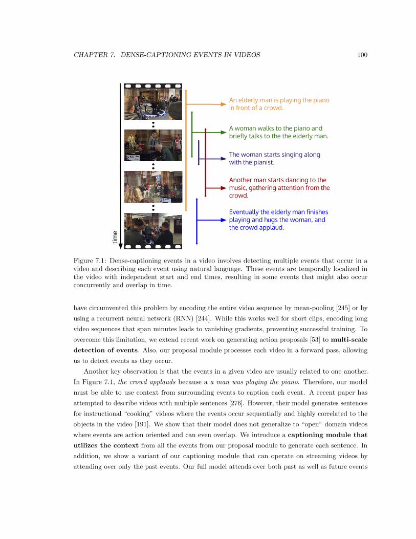
CHAPTER 7. DENSE-CAPTIONING EVENTS IN VIDEOS 100
An elderly man is playing the piano in front of a crowd.
Another man starts dancing to the music, gathering attention from the crowd.
Eventually the elderly man finishes playing and hugs the woman, and the crowd applaud.
A woman walks to the piano and briefly talks to the the elderly man.
time
The woman starts singing along with the pianist.
Figure 7.1: Dense-captioning events in a video involves detecting multiple events that occur in avideo and describing each event using natural language. These events are temporally localized inthe video with independent start and end times, resulting in some events that might also occurconcurrently and overlap in time.
have circumvented this problem by encoding the entire video sequence by mean-pooling [245] or by
using a recurrent neural network (RNN) [244]. While this works well for short clips, encoding long
video sequences that span minutes leads to vanishing gradients, preventing successful training. To
overcome this limitation, we extend recent work on generating action proposals [53] to multi-scale
detection of events. Also, our proposal module processes each video in a forward pass, allowing
us to detect events as they occur.
Another key observation is that the events in a given video are usually related to one another.
In Figure 7.1, the crowd applauds because a a man was playing the piano. Therefore, our model
must be able to use context from surrounding events to caption each event. A recent paper has
attempted to describe videos with multiple sentences [276]. However, their model generates sentences
for instructional “cooking” videos where the events occur sequentially and highly correlated to the
objects in the video [191]. We show that their model does not generalize to “open” domain videos
where events are action oriented and can even overlap. We introduce a captioning module that
utilizes the context from all the events from our proposal module to generate each sentence. In
addition, we show a variant of our captioning module that can operate on streaming videos by
attending over only the past events. Our full model attends over both past as well as future events
CHAPTER 7. DENSE-CAPTIONING EVENTS IN VIDEOS 101
and demonstrates the importance of using context.
To evaluate our model and benchmark progress in dense-captioning events, we introduce the
ActivityNet Captions dataset1. ActivityNet Captions contains 20k videos taken from ActivityNet [22],
where each video is annotated with a series of temporally localized descriptions (Figure 7.1). To
showcase long term event detection, our dataset contains videos as long as 10 minutes, with each
video annotated with on average 3.65 sentences. The descriptions refer to events that might be
simultaneously occurring, causing the video segments to overlap. We ensure that each description in
a given video is unique and refers to only one segment. While our videos are centered around human
activities, the descriptions may also refer to non-human events such as: two hours later, the mixture
becomes a delicious cake to eat. We collect our descriptions using crowdsourcing find that there is
high agreement in the temporal event segments, which is in line with research suggesting that brain
activity is naturally structured into semantically meaningful events [5].
With ActivityNet Captions, we are able to provide the first results for the task of dense-captioning
events. Together with our online proposal module and our online captioning module, we show that
we can detect and describe events in long or even streaming videos. We demonstrate that we are
able to detect events found in short clips as well as in long video sequences. Furthermore, we show
that utilizing context from other events in the video improves dense-captioning events. Finally,
we demonstrate how ActivityNet Captions can be used to study video retrieval as well as event
localization.
7.2 Related work
Dense-captioning events bridges two separate bodies of work: temporal action proposals and video
captioning. First, we review related work on action recognition, action detection and temporal
proposals. Next, we survey how video captioning started from video retrieval and video summarization,
leading to single-sentence captioning work. Finally, we contrast our work with recent work in
captioning images and videos with multiple sentences.
Early work in activity recognition involved using hidden Markov models to learn latent action
states [266], followed by discriminative SVM models that used key poses and action grammars [166,
240, 181]. Similar works have used hand-crafted features [194] or object-centric features [165] to
recognize actions in fixed camera settings. More recent works have used dense trajectories [253] or
deep learning features [106] to study actions. While our work is similar to these methods, we focus
on describing such events with natural language instead of a fixed label set.
To enable action localization, temporal action proposal methods started from traditional
sliding window approaches [52] and later started building models to propose a handful of possible
action segments [53, 23]. These proposal methods have used dictionary learning [23] or RNN
1The dataset is available at http://cs.stanford.edu/people/ranjaykrishna/densevid/. For a detailedanalysis of our dataset, please see our supplementary material.
CHAPTER 7. DENSE-CAPTIONING EVENTS IN VIDEOS 102
architectures [53] to find possible segments of interest. However, such methods required each video
frame to be processed once for every sliding window. DAPs introduced a framework to allow proposing
overlapping segments using a sliding window. We modify this framework by removing the sliding
windows and outputting proposals at every time step in a single pass of the video. We further extend
this model and enable it to detect long events by implementing a multi-scale version of DAPs, where
we sample frames at longer strides.
Orthogonal to work studying proposals, early approaches that connected video with language
studied the task of video retrieval with natural language. They worked on generating a common
embedding space between language and videos [171, 265]. Similar to these, we evaluate how well
existing models perform on our dataset. Additionally, we introduce the task of localizing a given
sentence given a video frame, allowing us to now also evaluate whether our models are able to locate
specified events.
In an effort to start describing videos, methods in video summarization aimed to congregate
segments of videos that include important or interesting visual information [273, 267, 80, 12]. These
methods attempted to use low level features such as color and motion or attempted to model
objects [279] and their relationships [259, 74] to select key segments. Meanwhile, others have utilized
text inputs from user studies to guide the selection process [224, 143]. While these summaries provide
a means of finding important segments, these methods are limited by small vocabularies and do not
evaluate how well we can explain visual events [274].
After these summarization works, early attempts at video captioning [245] simply mean-pooled
video frame features and used a pipeline inspired by the success of image captioning [109]. However,
this approach only works for short video clips with only one major event. To avoid this issue, others
have proposed either a recurrent encoder [49, 244, 262] or an attention mechanism [272]. To capture
more detail in videos, a new paper has recommended describing videos with paragraphs (a list of
sentences) using a hierarchical RNN [159] where the top level network generates a series of hidden
vectors that are used to initialize low level RNNs that generate each individual sentence [276]. While
our paper is most similar to this work, we address two important missing factors. First, the sentences
that their model generates refer to different events in the video but are not localized in time. Second,
they use the TACoS-MultiLevel [191], which contains less than 200 videos and is constrained to
“cooking” videos and only contain non-overlapping sequential events. We address these issues by
introducing the ActivityNet Captions dataset which contains overlapping events and by introducing
our captioning module that uses temporal context to capture the interdependency between all the
events in a video.
Finally, we build upon the recent work on dense-image-captioning [101], which generates a set
of localized descriptions for an image. Further work for this task has used spatial context to improve
captioning [268, 264]. Inspired by this work, and by recent literature on using spatial attention
to improve human tracking [1], we design our captioning module to incorporate temporal context
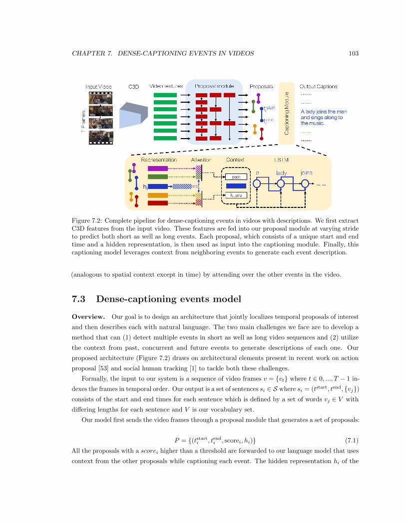
CHAPTER 7. DENSE-CAPTIONING EVENTS IN VIDEOS 103
Figure 7.2: Complete pipeline for dense-captioning events in videos with descriptions. We first extractC3D features from the input video. These features are fed into our proposal module at varying strideto predict both short as well as long events. Each proposal, which consists of a unique start and endtime and a hidden representation, is then used as input into the captioning module. Finally, thiscaptioning model leverages context from neighboring events to generate each event description.
(analogous to spatial context except in time) by attending over the other events in the video.
7.3 Dense-captioning events model
Overview. Our goal is to design an architecture that jointly localizes temporal proposals of interest
and then describes each with natural language. The two main challenges we face are to develop a
method that can (1) detect multiple events in short as well as long video sequences and (2) utilize
the context from past, concurrent and future events to generate descriptions of each one. Our
proposed architecture (Figure 7.2) draws on architectural elements present in recent work on action
proposal [53] and social human tracking [1] to tackle both these challenges.
Formally, the input to our system is a sequence of video frames v = {vt} where t ∈ 0, ..., T − 1 in-
dexes the frames in temporal order. Our output is a set of sentences si ∈ S where si = (tstart, tend, {vj})consists of the start and end times for each sentence which is defined by a set of words vj ∈ V with
differing lengths for each sentence and V is our vocabulary set.
Our model first sends the video frames through a proposal module that generates a set of proposals:
P = {(tstarti , tendi , scorei, hi)} (7.1)
All the proposals with a scorei higher than a threshold are forwarded to our language model that uses
context from the other proposals while captioning each event. The hidden representation hi of the
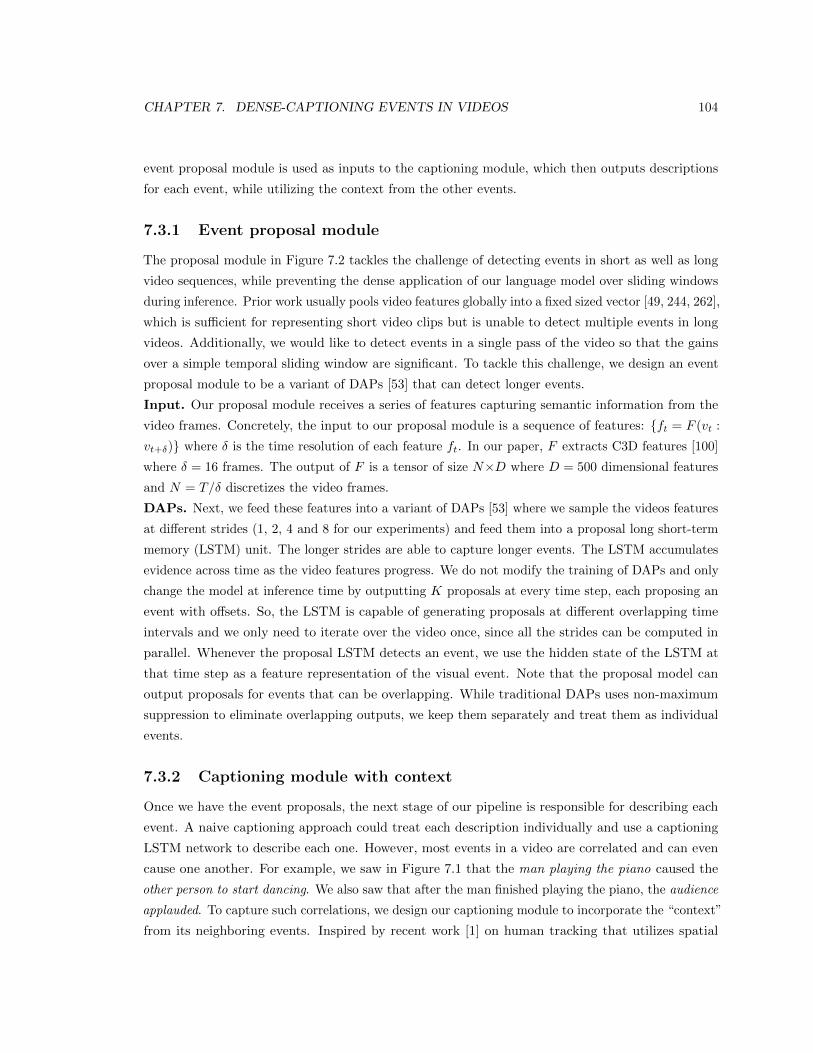
CHAPTER 7. DENSE-CAPTIONING EVENTS IN VIDEOS 104
event proposal module is used as inputs to the captioning module, which then outputs descriptions
for each event, while utilizing the context from the other events.
7.3.1 Event proposal module
The proposal module in Figure 7.2 tackles the challenge of detecting events in short as well as long
video sequences, while preventing the dense application of our language model over sliding windows
during inference. Prior work usually pools video features globally into a fixed sized vector [49, 244, 262],
which is sufficient for representing short video clips but is unable to detect multiple events in long
videos. Additionally, we would like to detect events in a single pass of the video so that the gains
over a simple temporal sliding window are significant. To tackle this challenge, we design an event
proposal module to be a variant of DAPs [53] that can detect longer events.
Input. Our proposal module receives a series of features capturing semantic information from the
video frames. Concretely, the input to our proposal module is a sequence of features: {ft = F (vt :
vt+δ)} where δ is the time resolution of each feature ft. In our paper, F extracts C3D features [100]
where δ = 16 frames. The output of F is a tensor of size N×D where D = 500 dimensional features
and N = T/δ discretizes the video frames.
DAPs. Next, we feed these features into a variant of DAPs [53] where we sample the videos features
at different strides (1, 2, 4 and 8 for our experiments) and feed them into a proposal long short-term
memory (LSTM) unit. The longer strides are able to capture longer events. The LSTM accumulates
evidence across time as the video features progress. We do not modify the training of DAPs and only
change the model at inference time by outputting K proposals at every time step, each proposing an
event with offsets. So, the LSTM is capable of generating proposals at different overlapping time
intervals and we only need to iterate over the video once, since all the strides can be computed in
parallel. Whenever the proposal LSTM detects an event, we use the hidden state of the LSTM at
that time step as a feature representation of the visual event. Note that the proposal model can
output proposals for events that can be overlapping. While traditional DAPs uses non-maximum
suppression to eliminate overlapping outputs, we keep them separately and treat them as individual
events.
7.3.2 Captioning module with context
Once we have the event proposals, the next stage of our pipeline is responsible for describing each
event. A naive captioning approach could treat each description individually and use a captioning
LSTM network to describe each one. However, most events in a video are correlated and can even
cause one another. For example, we saw in Figure 7.1 that the man playing the piano caused the
other person to start dancing. We also saw that after the man finished playing the piano, the audience
applauded. To capture such correlations, we design our captioning module to incorporate the “context”
from its neighboring events. Inspired by recent work [1] on human tracking that utilizes spatial
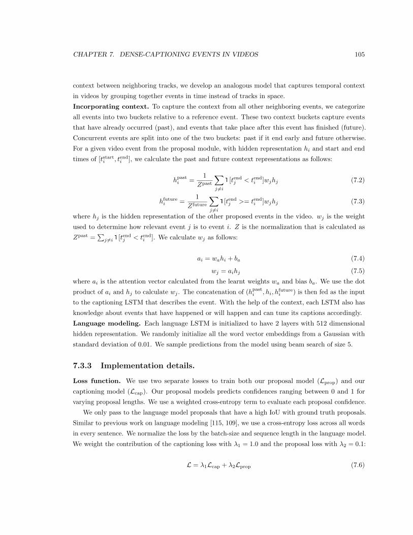
CHAPTER 7. DENSE-CAPTIONING EVENTS IN VIDEOS 105
context between neighboring tracks, we develop an analogous model that captures temporal context
in videos by grouping together events in time instead of tracks in space.
Incorporating context. To capture the context from all other neighboring events, we categorize
all events into two buckets relative to a reference event. These two context buckets capture events
that have already occurred (past), and events that take place after this event has finished (future).
Concurrent events are split into one of the two buckets: past if it end early and future otherwise.
For a given video event from the proposal module, with hidden representation hi and start and end
times of [tstarti , tendi ], we calculate the past and future context representations as follows:
hpasti =1
Zpast
∑j 6=i
1[tendj < tendi ]wjhj (7.2)
hfuturei =1
Zfuture
∑j 6=i
1[tendj >= tendi ]wjhj (7.3)
where hj is the hidden representation of the other proposed events in the video. wj is the weight
used to determine how relevant event j is to event i. Z is the normalization that is calculated as
Zpast =∑j 6=i 1[tendj < tendi ]. We calculate wj as follows:
ai = wahi + ba (7.4)
wj = aihj (7.5)
where ai is the attention vector calculated from the learnt weights wa and bias ba. We use the dot
product of ai and hj to calculate wj . The concatenation of (hpasti , hi, hfuturei ) is then fed as the input
to the captioning LSTM that describes the event. With the help of the context, each LSTM also has
knowledge about events that have happened or will happen and can tune its captions accordingly.
Language modeling. Each language LSTM is initialized to have 2 layers with 512 dimensional
hidden representation. We randomly initialize all the word vector embeddings from a Gaussian with
standard deviation of 0.01. We sample predictions from the model using beam search of size 5.
7.3.3 Implementation details.
Loss function. We use two separate losses to train both our proposal model (Lprop) and our
captioning model (Lcap). Our proposal models predicts confidences ranging between 0 and 1 for
varying proposal lengths. We use a weighted cross-entropy term to evaluate each proposal confidence.
We only pass to the language model proposals that have a high IoU with ground truth proposals.
Similar to previous work on language modeling [115, 109], we use a cross-entropy loss across all words
in every sentence. We normalize the loss by the batch-size and sequence length in the language model.
We weight the contribution of the captioning loss with λ1 = 1.0 and the proposal loss with λ2 = 0.1:
L = λ1Lcap + λ2Lprop (7.6)
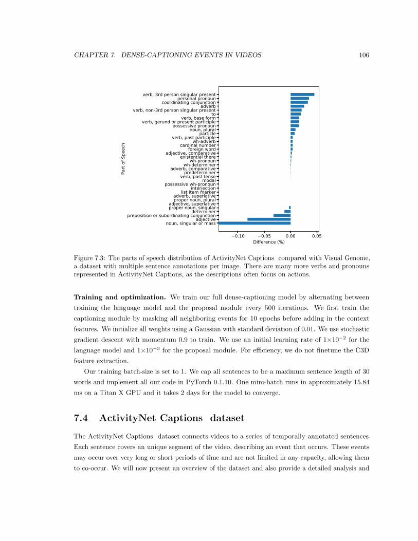
CHAPTER 7. DENSE-CAPTIONING EVENTS IN VIDEOS 106
0.10 0.05 0.00 0.05Difference (%)
noun, singular or massadjective
preposition or subordinating conjunctiondeterminer
proper noun, singularadjective, superlative
proper noun, pluraladverb, superlative
list item markerinterjection
possessive wh-pronounmodal
verb, past tensepredeterminer
adverb, comparativewh-determiner
wh-pronounexistential there
adjective, comparativeforeign word
cardinal numberwh-adverb
verb, past participleparticle
noun, pluralpossessive pronoun
verb, gerund or present participleverb, base form
toverb, non-3rd person singular present
adverbcoordinating conjunction
personal pronounverb, 3rd person singular present
Part
of S
peec
h
Figure 7.3: The parts of speech distribution of ActivityNet Captions compared with Visual Genome,a dataset with multiple sentence annotations per image. There are many more verbs and pronounsrepresented in ActivityNet Captions, as the descriptions often focus on actions.
Training and optimization. We train our full dense-captioning model by alternating between
training the language model and the proposal module every 500 iterations. We first train the
captioning module by masking all neighboring events for 10 epochs before adding in the context
features. We initialize all weights using a Gaussian with standard deviation of 0.01. We use stochastic
gradient descent with momentum 0.9 to train. We use an initial learning rate of 1×10⁻² for the
language model and 1×10⁻³ for the proposal module. For efficiency, we do not finetune the C3D
feature extraction.
Our training batch-size is set to 1. We cap all sentences to be a maximum sentence length of 30
words and implement all our code in PyTorch 0.1.10. One mini-batch runs in approximately 15.84
ms on a Titan X GPU and it takes 2 days for the model to converge.
7.4 ActivityNet Captions dataset
The ActivityNet Captions dataset connects videos to a series of temporally annotated sentences.
Each sentence covers an unique segment of the video, describing an event that occurs. These events
may occur over very long or short periods of time and are not limited in any capacity, allowing them
to co-occur. We will now present an overview of the dataset and also provide a detailed analysis and
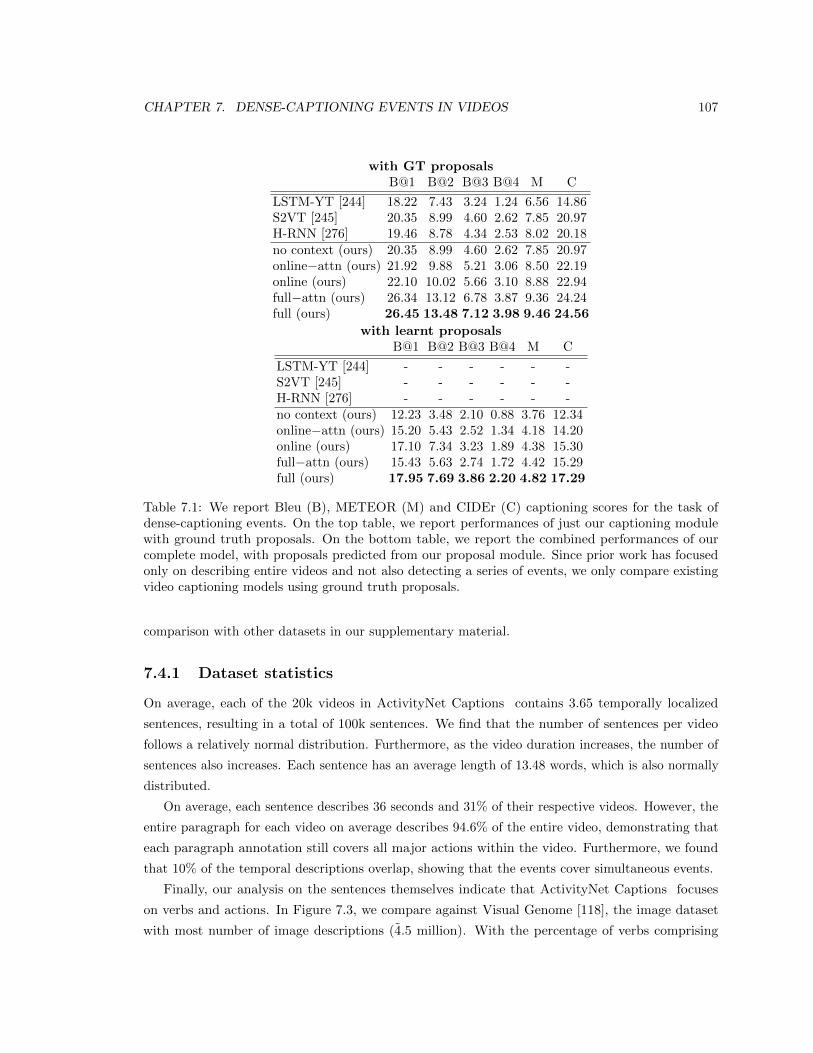
CHAPTER 7. DENSE-CAPTIONING EVENTS IN VIDEOS 107
with GT proposalsB@1 B@2 B@3 B@4 M C
LSTM-YT [244] 18.22 7.43 3.24 1.24 6.56 14.86S2VT [245] 20.35 8.99 4.60 2.62 7.85 20.97H-RNN [276] 19.46 8.78 4.34 2.53 8.02 20.18no context (ours) 20.35 8.99 4.60 2.62 7.85 20.97online−attn (ours) 21.92 9.88 5.21 3.06 8.50 22.19online (ours) 22.10 10.02 5.66 3.10 8.88 22.94full−attn (ours) 26.34 13.12 6.78 3.87 9.36 24.24full (ours) 26.45 13.48 7.12 3.98 9.46 24.56
with learnt proposalsB@1 B@2 B@3 B@4 M C
LSTM-YT [244] - - - - - -S2VT [245] - - - - - -H-RNN [276] - - - - - -no context (ours) 12.23 3.48 2.10 0.88 3.76 12.34online−attn (ours) 15.20 5.43 2.52 1.34 4.18 14.20online (ours) 17.10 7.34 3.23 1.89 4.38 15.30full−attn (ours) 15.43 5.63 2.74 1.72 4.42 15.29full (ours) 17.95 7.69 3.86 2.20 4.82 17.29
Table 7.1: We report Bleu (B), METEOR (M) and CIDEr (C) captioning scores for the task ofdense-captioning events. On the top table, we report performances of just our captioning modulewith ground truth proposals. On the bottom table, we report the combined performances of ourcomplete model, with proposals predicted from our proposal module. Since prior work has focusedonly on describing entire videos and not also detecting a series of events, we only compare existingvideo captioning models using ground truth proposals.
comparison with other datasets in our supplementary material.
7.4.1 Dataset statistics
On average, each of the 20k videos in ActivityNet Captions contains 3.65 temporally localized
sentences, resulting in a total of 100k sentences. We find that the number of sentences per video
follows a relatively normal distribution. Furthermore, as the video duration increases, the number of
sentences also increases. Each sentence has an average length of 13.48 words, which is also normally
distributed.
On average, each sentence describes 36 seconds and 31% of their respective videos. However, the
entire paragraph for each video on average describes 94.6% of the entire video, demonstrating that
each paragraph annotation still covers all major actions within the video. Furthermore, we found
that 10% of the temporal descriptions overlap, showing that the events cover simultaneous events.
Finally, our analysis on the sentences themselves indicate that ActivityNet Captions focuses
on verbs and actions. In Figure 7.3, we compare against Visual Genome [118], the image dataset
with most number of image descriptions (4.5 million). With the percentage of verbs comprising
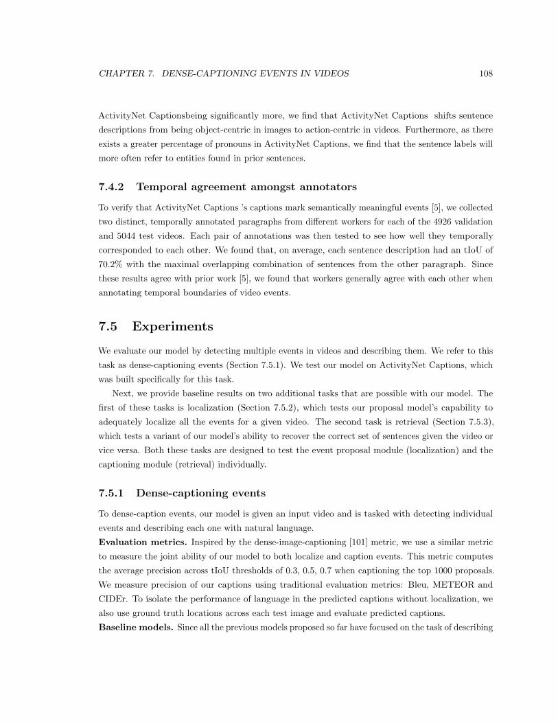
CHAPTER 7. DENSE-CAPTIONING EVENTS IN VIDEOS 108
ActivityNet Captionsbeing significantly more, we find that ActivityNet Captions shifts sentence
descriptions from being object-centric in images to action-centric in videos. Furthermore, as there
exists a greater percentage of pronouns in ActivityNet Captions, we find that the sentence labels will
more often refer to entities found in prior sentences.
7.4.2 Temporal agreement amongst annotators
To verify that ActivityNet Captions ’s captions mark semantically meaningful events [5], we collected
two distinct, temporally annotated paragraphs from different workers for each of the 4926 validation
and 5044 test videos. Each pair of annotations was then tested to see how well they temporally
corresponded to each other. We found that, on average, each sentence description had an tIoU of
70.2% with the maximal overlapping combination of sentences from the other paragraph. Since
these results agree with prior work [5], we found that workers generally agree with each other when
annotating temporal boundaries of video events.
7.5 Experiments
We evaluate our model by detecting multiple events in videos and describing them. We refer to this
task as dense-captioning events (Section 7.5.1). We test our model on ActivityNet Captions, which
was built specifically for this task.
Next, we provide baseline results on two additional tasks that are possible with our model. The
first of these tasks is localization (Section 7.5.2), which tests our proposal model’s capability to
adequately localize all the events for a given video. The second task is retrieval (Section 7.5.3),
which tests a variant of our model’s ability to recover the correct set of sentences given the video or
vice versa. Both these tasks are designed to test the event proposal module (localization) and the
captioning module (retrieval) individually.
7.5.1 Dense-captioning events
To dense-caption events, our model is given an input video and is tasked with detecting individual
events and describing each one with natural language.
Evaluation metrics. Inspired by the dense-image-captioning [101] metric, we use a similar metric
to measure the joint ability of our model to both localize and caption events. This metric computes
the average precision across tIoU thresholds of 0.3, 0.5, 0.7 when captioning the top 1000 proposals.
We measure precision of our captions using traditional evaluation metrics: Bleu, METEOR and
CIDEr. To isolate the performance of language in the predicted captions without localization, we
also use ground truth locations across each test image and evaluate predicted captions.
Baseline models. Since all the previous models proposed so far have focused on the task of describing
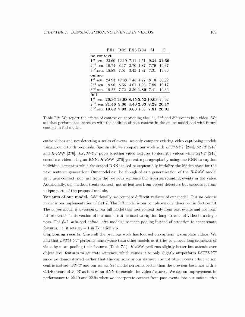
CHAPTER 7. DENSE-CAPTIONING EVENTS IN VIDEOS 109
B@1 B@2 B@3 B@4 M C
no context1st sen. 23.60 12.19 7.11 4.51 9.34 31.562nd sen. 19.74 8.17 3.76 1.87 7.79 19.373rd sen. 18.89 7.51 3.43 1.87 7.31 19.36online1st sen. 24.93 12.38 7.45 4.77 8.10 30.922nd sen. 19.96 8.66 4.01 1.93 7.88 19.173rd sen. 19.22 7.72 3.56 1.89 7.41 19.36full1st sen. 26.33 13.98 8.45 5.52 10.03 29.922nd sen. 21.46 9.06 4.40 2.33 8.28 20.173rd sen. 19.82 7.93 3.63 1.83 7.81 20.01
Table 7.2: We report the effects of context on captioning the 1st, 2nd and 3rd events in a video. Wesee that performance increases with the addition of past context in the online model and with futurecontext in full model.
entire videos and not detecting a series of events, we only compare existing video captioning models
using ground truth proposals. Specifically, we compare our work with LSTM-YT [244], S2VT [245]
and H-RNN [276]. LSTM-YT pools together video features to describe videos while S2VT [245]
encodes a video using an RNN. H-RNN [276] generates paragraphs by using one RNN to caption
individual sentences while the second RNN is used to sequentially initialize the hidden state for the
next sentence generation. Our model can be though of as a generalization of the H-RNN model
as it uses context, not just from the previous sentence but from surrounding events in the video.
Additionally, our method treats context, not as features from object detectors but encodes it from
unique parts of the proposal module.
Variants of our model. Additionally, we compare different variants of our model. Our no context
model is our implementation of S2VT. The full model is our complete model described in Section 7.3.
The online model is a version of our full model that uses context only from past events and not from
future events. This version of our model can be used to caption long streams of video in a single
pass. The full−attn and online−attn models use mean pooling instead of attention to concatenate
features, i.e. it sets wj = 1 in Equation 7.5.
Captioning results. Since all the previous work has focused on captioning complete videos, We
find that LSTM-YT performs much worse than other models as it tries to encode long sequences of
video by mean pooling their features (Table 7.1). H-RNN performs slightly better but attends over
object level features to generate sentence, which causes it to only slightly outperform LSTM-YT
since we demonstrated earlier that the captions in our dataset are not object centric but action
centric instead. S2VT and our no context model performs better than the previous baselines with a
CIDEr score of 20.97 as it uses an RNN to encode the video features. We see an improvement in
performance to 22.19 and 22.94 when we incorporate context from past events into our online−attn
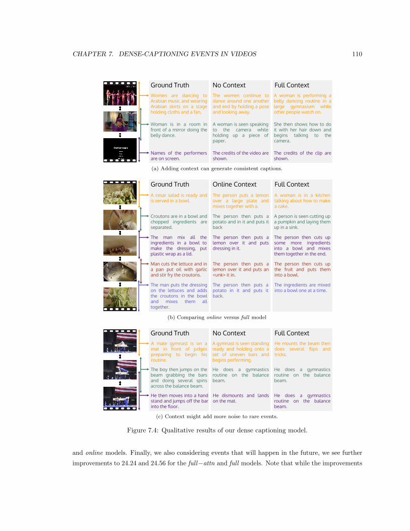
CHAPTER 7. DENSE-CAPTIONING EVENTS IN VIDEOS 110
Ground Truth No Context Full ContextWomen are dancing toArabian music and wearingArabian skirts on a stageholding cloths and a fan.
The women continue todance around one anotherand end by holding a poseand looking away.
A woman is performing abelly dancing routine in alarge gymnasium whileother people watch on.
Woman is in a room infront of a mirror doing thebelly dance.
A woman is seen speakingto the camera whileholding up a piece ofpaper.
She then shows how to doit with her hair down andbegins talking to thecamera.
Names of the performersare on screen.
The credits of the video areshown.
The credits of the clip areshown.
(a) Adding context can generate consistent captions.
Ground Truth Online Context Full Context
A cesar salad is ready andis served in a bowl.
The person puts a lemonover a large plate andmixes together with a.
A woman is in a kitchentalking about how to makea cake.
Croutons are in a bowl andchopped ingredients areseparated.
The person then puts apotato and in it and puts itback
A person is seen cutting upa pumpkin and laying themup in a sink.
The man mix all theingredients in a bowl tomake the dressing, putplastic wrap as a lid.
The person then puts alemon over it and putsdressing in it.
The person then cuts upsome more ingredientsinto a bowl and mixesthem together in the end.
Man cuts the lettuce and ina pan put oil with garlicand stir fry the croutons.
The person then puts alemon over it and puts an<unk> it in.
The person then cuts upthe fruit and puts theminto a bowl.
The man puts the dressingon the lettuces and addsthe croutons in the bowland mixes them alltogether.
The person then puts apotato in it and puts itback.
The ingredients are mixedinto a bowl one at a time.
(b) Comparing online versus full model
Ground Truth No Context Full ContextA male gymnast is on amat in front of judgespreparing to begin hisroutine.
A gymnast is seen standingready and holding onto aset of uneven bars andbegins performing.
He mounts the beam thendoes several flips andtricks.
The boy then jumps on thebeam grabbing the barsand doing several spinsacross the balance beam.
He does a gymnasticsroutine on the balancebeam.
He does a gymnasticsroutine on the balancebeam.
He then moves into a handstand and jumps off the barinto the floor.
He dismounts and landson the mat.
He does a gymnasticsroutine on the balancebeam.
(c) Context might add more noise to rare events.
Figure 7.4: Qualitative results of our dense captioning model.
and online models. Finally, we also considering events that will happen in the future, we see further
improvements to 24.24 and 24.56 for the full−attn and full models. Note that while the improvements
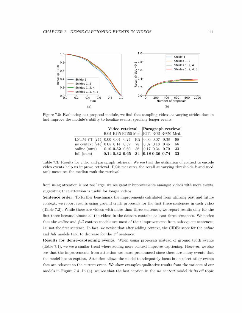
CHAPTER 7. DENSE-CAPTIONING EVENTS IN VIDEOS 111
0.0 0.2 0.4 0.6 0.8 1.0tIoU
0.0
0.2
0.4
0.6
0.8
1.0Re
call
@ 1
000
Stride 1Strides 1, 2Strides 1, 2, 4Strides 1, 2, 4, 8
(a)
0 200 400 600 800 1000Number of proposals
0.0
0.2
0.4
0.6
0.8
1.0
Reca
ll @
tIoU
=0.8
Stride 1Strides 1, 2Strides 1, 2, 4Strides 1, 2, 4, 8
(b)
Figure 7.5: Evaluating our proposal module, we find that sampling videos at varying strides does infact improve the module’s ability to localize events, specially longer events.
Video retrieval Paragraph retrievalR@1 R@5 R@50 Med. R@1 R@5 R@50 Med.
LSTM-YT [244] 0.00 0.04 0.24 102 0.00 0.07 0.38 98no context [245] 0.05 0.14 0.32 78 0.07 0.18 0.45 56online (ours) 0.10 0.32 0.60 36 0.17 0.34 0.70 33full (ours) 0.14 0.32 0.65 34 0.18 0.36 0.74 32
Table 7.3: Results for video and paragraph retrieval. We see that the utilization of context to encodevideo events help us improve retrieval. R@k measures the recall at varying thresholds k and med.rank measures the median rank the retrieval.
from using attention is not too large, we see greater improvements amongst videos with more events,
suggesting that attention is useful for longer videos.
Sentence order. To further benchmark the improvements calculated from utilizing past and future
context, we report results using ground truth proposals for the first three sentences in each video
(Table 7.2). While there are videos with more than three sentences, we report results only for the
first three because almost all the videos in the dataset contains at least three sentences. We notice
that the online and full context models see most of their improvements from subsequent sentences,
i.e. not the first sentence. In fact, we notice that after adding context, the CIDEr score for the online
and full models tend to decrease for the 1st sentence.
Results for dense-captioning events. When using proposals instead of ground truth events
(Table 7.1), we see a similar trend where adding more context improves captioning. However, we also
see that the improvements from attention are more pronounced since there are many events that
the model has to caption. Attention allows the model to adequately focus in on select other events
that are relevant to the current event. We show examples qualitative results from the variants of our
models in Figure 7.4. In (a), we see that the last caption in the no context model drifts off topic
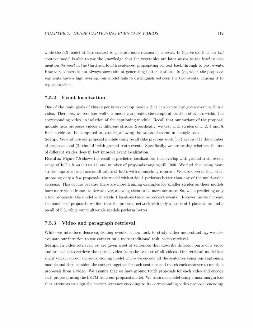
CHAPTER 7. DENSE-CAPTIONING EVENTS IN VIDEOS 112
while the full model utilizes context to generate more reasonable context. In (c), we see that our full
context model is able to use the knowledge that the vegetables are later mixed in the bowl to also
mention the bowl in the third and fourth sentences, propagating context back through to past events.
However, context is not always successful at generating better captions. In (c), when the proposed
segments have a high overlap, our model fails to distinguish between the two events, causing it to
repeat captions.
7.5.2 Event localization
One of the main goals of this paper is to develop models that can locate any given event within a
video. Therefore, we test how well our model can predict the temporal location of events within the
corresponding video, in isolation of the captioning module. Recall that our variant of the proposal
module uses proposes videos at different strides. Specifically, we test with strides of 1, 2, 4 and 8.
Each stride can be computed in parallel, allowing the proposal to run in a single pass.
Setup. We evaluate our proposal module using recall (like previous work [53]) against (1) the number
of proposals and (2) the IoU with ground truth events. Specifically, we are testing whether, the use
of different strides does in fact improve event localization.
Results. Figure 7.5 shows the recall of predicted localizations that overlap with ground truth over a
range of IoU’s from 0.0 to 1.0 and number of proposals ranging till 1000. We find that using more
strides improves recall across all values of IoU’s with diminishing returns . We also observe that when
proposing only a few proposals, the model with stride 1 performs better than any of the multi-stride
versions. This occurs because there are more training examples for smaller strides as these models
have more video frames to iterate over, allowing them to be more accurate. So, when predicting only
a few proposals, the model with stride 1 localizes the most correct events. However, as we increase
the number of proposals, we find that the proposal network with only a stride of 1 plateaus around a
recall of 0.3, while our multi-scale models perform better.
7.5.3 Video and paragraph retrieval
While we introduce dense-captioning events, a new task to study video understanding, we also
evaluate our intuition to use context on a more traditional task: video retrieval.
Setup. In video retrieval, we are given a set of sentences that describe different parts of a video
and are asked to retrieve the correct video from the test set of all videos. Our retrieval model is a
slight variant on our dense-captioning model where we encode all the sentences using our captioning
module and then combine the context together for each sentence and match each sentence to multiple
proposals from a video. We assume that we have ground truth proposals for each video and encode
each proposal using the LSTM from our proposal model. We train our model using a max-margin loss
that attempts to align the correct sentence encoding to its corresponding video proposal encoding.
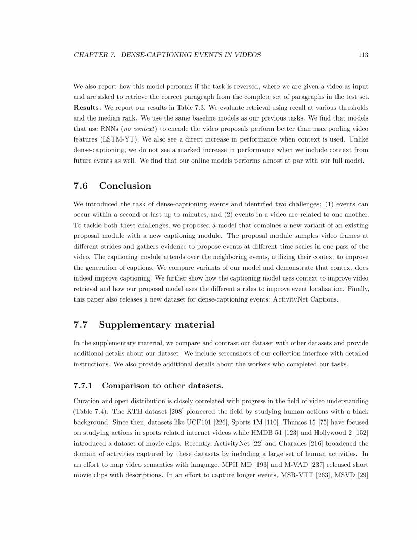
CHAPTER 7. DENSE-CAPTIONING EVENTS IN VIDEOS 113
We also report how this model performs if the task is reversed, where we are given a video as input
and are asked to retrieve the correct paragraph from the complete set of paragraphs in the test set.
Results. We report our results in Table 7.3. We evaluate retrieval using recall at various thresholds
and the median rank. We use the same baseline models as our previous tasks. We find that models
that use RNNs (no context) to encode the video proposals perform better than max pooling video
features (LSTM-YT). We also see a direct increase in performance when context is used. Unlike
dense-captioning, we do not see a marked increase in performance when we include context from
future events as well. We find that our online models performs almost at par with our full model.
7.6 Conclusion
We introduced the task of dense-captioning events and identified two challenges: (1) events can
occur within a second or last up to minutes, and (2) events in a video are related to one another.
To tackle both these challenges, we proposed a model that combines a new variant of an existing
proposal module with a new captioning module. The proposal module samples video frames at
different strides and gathers evidence to propose events at different time scales in one pass of the
video. The captioning module attends over the neighboring events, utilizing their context to improve
the generation of captions. We compare variants of our model and demonstrate that context does
indeed improve captioning. We further show how the captioning model uses context to improve video
retrieval and how our proposal model uses the different strides to improve event localization. Finally,
this paper also releases a new dataset for dense-captioning events: ActivityNet Captions.
7.7 Supplementary material
In the supplementary material, we compare and contrast our dataset with other datasets and provide
additional details about our dataset. We include screenshots of our collection interface with detailed
instructions. We also provide additional details about the workers who completed our tasks.
7.7.1 Comparison to other datasets.
Curation and open distribution is closely correlated with progress in the field of video understanding
(Table 7.4). The KTH dataset [208] pioneered the field by studying human actions with a black
background. Since then, datasets like UCF101 [226], Sports 1M [110], Thumos 15 [75] have focused
on studying actions in sports related internet videos while HMDB 51 [123] and Hollywood 2 [152]
introduced a dataset of movie clips. Recently, ActivityNet [22] and Charades [216] broadened the
domain of activities captured by these datasets by including a large set of human activities. In
an effort to map video semantics with language, MPII MD [193] and M-VAD [237] released short
movie clips with descriptions. In an effort to capture longer events, MSR-VTT [263], MSVD [29]
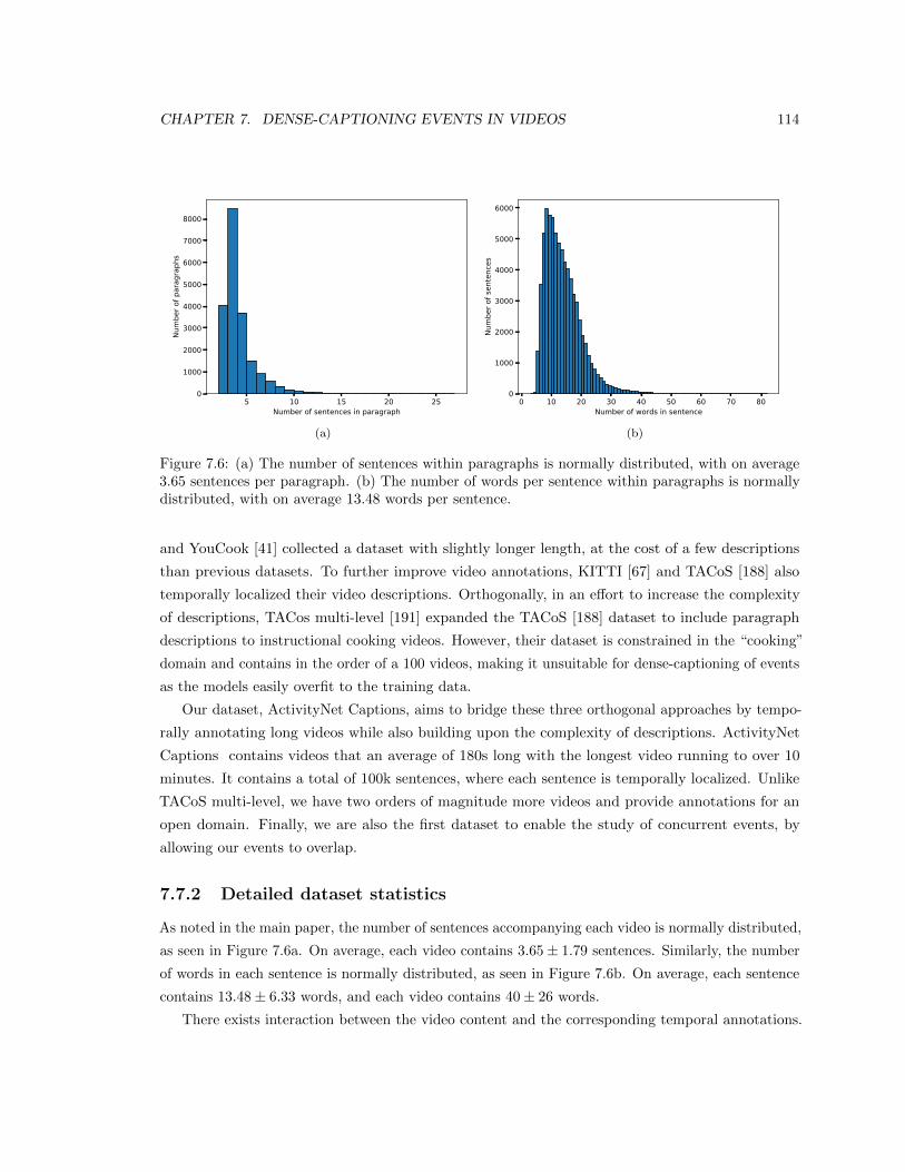
CHAPTER 7. DENSE-CAPTIONING EVENTS IN VIDEOS 114
5 10 15 20 25Number of sentences in paragraph
0
1000
2000
3000
4000
5000
6000
7000
8000
Num
ber o
f par
agra
phs
(a)
0 10 20 30 40 50 60 70 80Number of words in sentence
0
1000
2000
3000
4000
5000
6000
Num
ber o
f sen
tenc
es
(b)
Figure 7.6: (a) The number of sentences within paragraphs is normally distributed, with on average3.65 sentences per paragraph. (b) The number of words per sentence within paragraphs is normallydistributed, with on average 13.48 words per sentence.
and YouCook [41] collected a dataset with slightly longer length, at the cost of a few descriptions
than previous datasets. To further improve video annotations, KITTI [67] and TACoS [188] also
temporally localized their video descriptions. Orthogonally, in an effort to increase the complexity
of descriptions, TACos multi-level [191] expanded the TACoS [188] dataset to include paragraph
descriptions to instructional cooking videos. However, their dataset is constrained in the “cooking”
domain and contains in the order of a 100 videos, making it unsuitable for dense-captioning of events
as the models easily overfit to the training data.
Our dataset, ActivityNet Captions, aims to bridge these three orthogonal approaches by tempo-
rally annotating long videos while also building upon the complexity of descriptions. ActivityNet
Captions contains videos that an average of 180s long with the longest video running to over 10
minutes. It contains a total of 100k sentences, where each sentence is temporally localized. Unlike
TACoS multi-level, we have two orders of magnitude more videos and provide annotations for an
open domain. Finally, we are also the first dataset to enable the study of concurrent events, by
allowing our events to overlap.
7.7.2 Detailed dataset statistics
As noted in the main paper, the number of sentences accompanying each video is normally distributed,
as seen in Figure 7.6a. On average, each video contains 3.65± 1.79 sentences. Similarly, the number
of words in each sentence is normally distributed, as seen in Figure 7.6b. On average, each sentence
contains 13.48± 6.33 words, and each video contains 40± 26 words.
There exists interaction between the video content and the corresponding temporal annotations.
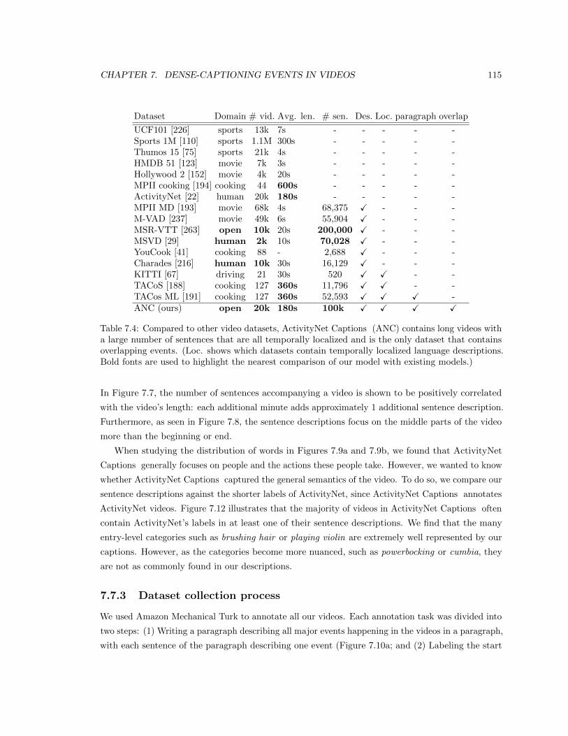
CHAPTER 7. DENSE-CAPTIONING EVENTS IN VIDEOS 115
Dataset Domain # vid. Avg. len. # sen. Des. Loc. paragraph overlap
UCF101 [226] sports 13k 7s - - - - -Sports 1M [110] sports 1.1M 300s - - - - -Thumos 15 [75] sports 21k 4s - - - - -HMDB 51 [123] movie 7k 3s - - - - -Hollywood 2 [152] movie 4k 20s - - - - -MPII cooking [194] cooking 44 600s - - - - -ActivityNet [22] human 20k 180s - - - - -MPII MD [193] movie 68k 4s 68,375 X - - -M-VAD [237] movie 49k 6s 55,904 X - - -MSR-VTT [263] open 10k 20s 200,000 X - - -MSVD [29] human 2k 10s 70,028 X - - -YouCook [41] cooking 88 - 2,688 X - - -Charades [216] human 10k 30s 16,129 X - - -KITTI [67] driving 21 30s 520 X X - -TACoS [188] cooking 127 360s 11,796 X X - -TACos ML [191] cooking 127 360s 52,593 X X X -ANC (ours) open 20k 180s 100k X X X X
Table 7.4: Compared to other video datasets, ActivityNet Captions (ANC) contains long videos witha large number of sentences that are all temporally localized and is the only dataset that containsoverlapping events. (Loc. shows which datasets contain temporally localized language descriptions.Bold fonts are used to highlight the nearest comparison of our model with existing models.)
In Figure 7.7, the number of sentences accompanying a video is shown to be positively correlated
with the video’s length: each additional minute adds approximately 1 additional sentence description.
Furthermore, as seen in Figure 7.8, the sentence descriptions focus on the middle parts of the video
more than the beginning or end.
When studying the distribution of words in Figures 7.9a and 7.9b, we found that ActivityNet
Captions generally focuses on people and the actions these people take. However, we wanted to know
whether ActivityNet Captions captured the general semantics of the video. To do so, we compare our
sentence descriptions against the shorter labels of ActivityNet, since ActivityNet Captions annotates
ActivityNet videos. Figure 7.12 illustrates that the majority of videos in ActivityNet Captions often
contain ActivityNet’s labels in at least one of their sentence descriptions. We find that the many
entry-level categories such as brushing hair or playing violin are extremely well represented by our
captions. However, as the categories become more nuanced, such as powerbocking or cumbia, they
are not as commonly found in our descriptions.
7.7.3 Dataset collection process
We used Amazon Mechanical Turk to annotate all our videos. Each annotation task was divided into
two steps: (1) Writing a paragraph describing all major events happening in the videos in a paragraph,
with each sentence of the paragraph describing one event (Figure 7.10a; and (2) Labeling the start
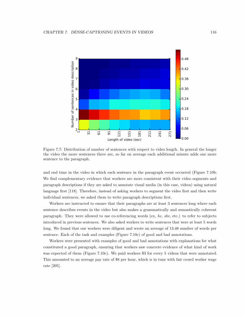
CHAPTER 7. DENSE-CAPTIONING EVENTS IN VIDEOS 116
1
31
61
91
12
1
15
1
18
1
21
1
24
1
27
1
Length of video (sec)
9
8
7
6
5
4
3
2
Num
ber
of
sente
nce
s in
vid
eo d
esc
ripti
on
0.00
0.06
0.12
0.18
0.24
0.30
0.36
0.42
0.48
Figure 7.7: Distribution of number of sentences with respect to video length. In general the longerthe video the more sentences there are, so far on average each additional minute adds one moresentence to the paragraph.
and end time in the video in which each sentence in the paragraph event occurred (Figure 7.10b.
We find complementary evidence that workers are more consistent with their video segments and
paragraph descriptions if they are asked to annotate visual media (in this case, videos) using natural
language first [118]. Therefore, instead of asking workers to segment the video first and then write
individual sentences, we asked them to write paragraph descriptions first.
Workers are instructed to ensure that their paragraphs are at least 3 sentences long where each
sentence describes events in the video but also makes a grammatically and semantically coherent
paragraph. They were allowed to use co-referencing words (ex, he, she, etc.) to refer to subjects
introduced in previous sentences. We also asked workers to write sentences that were at least 5 words
long. We found that our workers were diligent and wrote an average of 13.48 number of words per
sentence. Each of the task and examples (Figure 7.10c) of good and bad annotations.
Workers were presented with examples of good and bad annotations with explanations for what
constituted a good paragraph, ensuring that workers saw concrete evidence of what kind of work
was expected of them (Figure 7.10c). We paid workers $3 for every 5 videos that were annotated.
This amounted to an average pay rate of $8 per hour, which is in tune with fair crowd worker wage
rate [205].
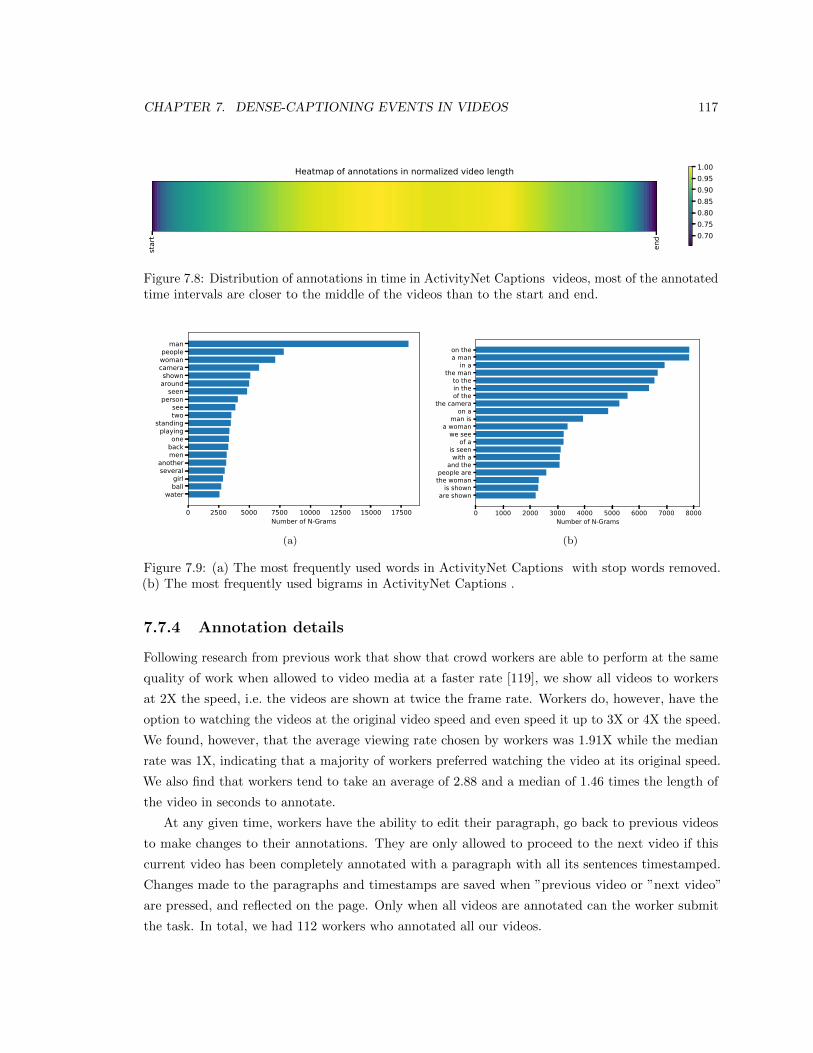
CHAPTER 7. DENSE-CAPTIONING EVENTS IN VIDEOS 117
star
t
end
Heatmap of annotations in normalized video length
0.700.750.800.850.900.951.00
Figure 7.8: Distribution of annotations in time in ActivityNet Captions videos, most of the annotatedtime intervals are closer to the middle of the videos than to the start and end.
0 2500 5000 7500 10000 12500 15000 17500Number of N-Grams
waterballgirl
severalanother
menbackone
playingstanding
twosee
personseen
aroundshown
camerawomanpeople
man
(a)
0 1000 2000 3000 4000 5000 6000 7000 8000Number of N-Grams
are shownis shown
the womanpeople are
and thewith a
is seenof a
we seea woman
man ison a
the cameraof thein theto the
the manin a
a manon the
(b)
Figure 7.9: (a) The most frequently used words in ActivityNet Captions with stop words removed.(b) The most frequently used bigrams in ActivityNet Captions .
7.7.4 Annotation details
Following research from previous work that show that crowd workers are able to perform at the same
quality of work when allowed to video media at a faster rate [119], we show all videos to workers
at 2X the speed, i.e. the videos are shown at twice the frame rate. Workers do, however, have the
option to watching the videos at the original video speed and even speed it up to 3X or 4X the speed.
We found, however, that the average viewing rate chosen by workers was 1.91X while the median
rate was 1X, indicating that a majority of workers preferred watching the video at its original speed.
We also find that workers tend to take an average of 2.88 and a median of 1.46 times the length of
the video in seconds to annotate.
At any given time, workers have the ability to edit their paragraph, go back to previous videos
to make changes to their annotations. They are only allowed to proceed to the next video if this
current video has been completely annotated with a paragraph with all its sentences timestamped.
Changes made to the paragraphs and timestamps are saved when ”previous video or ”next video”
are pressed, and reflected on the page. Only when all videos are annotated can the worker submit
the task. In total, we had 112 workers who annotated all our videos.
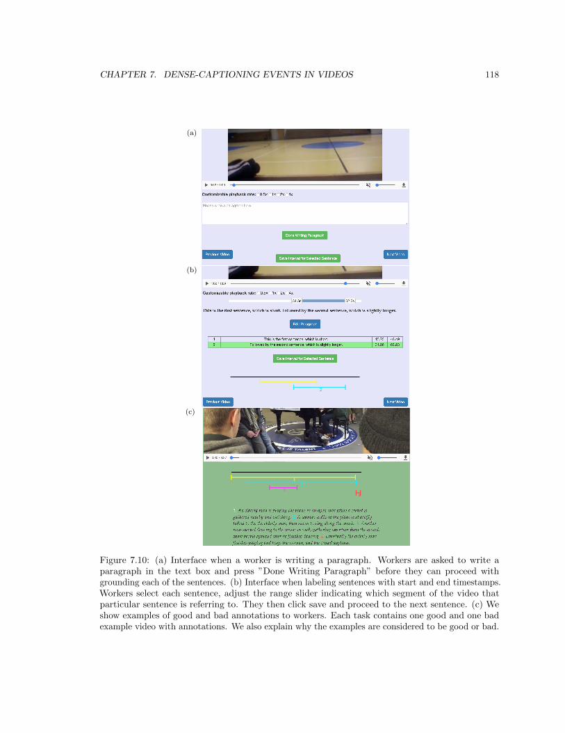
CHAPTER 7. DENSE-CAPTIONING EVENTS IN VIDEOS 118
(a)
(b)
(c)
Figure 7.10: (a) Interface when a worker is writing a paragraph. Workers are asked to write aparagraph in the text box and press ”Done Writing Paragraph” before they can proceed withgrounding each of the sentences. (b) Interface when labeling sentences with start and end timestamps.Workers select each sentence, adjust the range slider indicating which segment of the video thatparticular sentence is referring to. They then click save and proceed to the next sentence. (c) Weshow examples of good and bad annotations to workers. Each task contains one good and one badexample video with annotations. We also explain why the examples are considered to be good or bad.
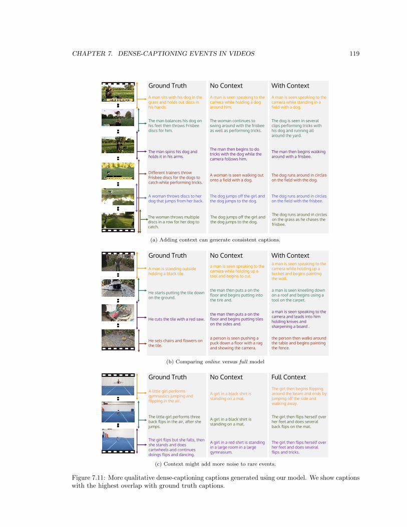
CHAPTER 7. DENSE-CAPTIONING EVENTS IN VIDEOS 119
Ground Truth No Context With ContextA man sits with his dog in the grass and holds out discs in his hands.
A man is seen speaking to the camera while holding a dog around him.
A man is seen speaking to the camera while standing in a field with a dog.
The man balances his dog on his feet then throws Frisbee discs for him.
The woman continues to swing around with the frisbeeas well as performing tricks.
The dog is seen in several clips performing tricks with his dog and running all around the yard.
The man spins his dog and holds it in his arms.
The man then begins to do tricks with the dog while the camera follows him.
The man then begins walking around with a frisbee.
Different trainers throw Frisbee discs for the dogs to catch while performing tricks.
A woman is seen walking out onto a field with a dog.
The dog runs around in circles on the field with the dog.
A woman throws discs to her dog that jumps from her back.
The dog jumps off the girl and the dog jumps to the dog.
The dog runs around in circles on the field with the frisbee.
The woman throws multiple discs in a row for her dog to catch.
The dog jumps off the girl and the dog jumps to the dog.
The dog runs around in circles on the grass as he chases the frisbee.
(a) Adding context can generate consistent captions.
Ground Truth No Context With Context
A man is standing outside holding a black tile.
a man is seen speaking to the camera while holding up a tool and begins to cut.
a man is seen speaking to the camera while holding up a bucket and begins painting the wall.
He starts putting the tile down on the ground.
the man then puts a on the floor and begins putting into the tire and.
a man is seen kneeling down on a roof and begins using a tool on the carpet.
He cuts the tile with a red saw.the man then puts a on the floor and begins putting tiles on the sides and.
a man is seen speaking to the camera and leads into him holding knives and sharpening a board .
He sets chairs and flowers on the tile.
a person is seen pushing a puck down a floor with a rag and showing the camera.
the person then walks around the table and begins painting the fence.
(b) Comparing online versus full model
Ground Truth No Context Full Context
A little girl performs gymnastics jumping and flipping in the air.
A girl in a black shirt is standing on a mat.
The girl then begins flipping around the beam and ends by jumping off the side and walking away.
The little girl performs three back flips in the air, after she jumps.
A girl in a black shirt is standing on a mat.
The girl then flips herself over her feet and does several back flips on the mat.
The girl flips but she falls, then she stands and does cartwheels and continues doings flips and dancing.
A girl in a red shirt is standing in a large room in a large gymnasium.
The girl then flips herself over her feet and does several flips and tricks.
(c) Context might add more noise to rare events.
Figure 7.11: More qualitative dense-captioning captions generated using our model. We show captionswith the highest overlap with ground truth captions.
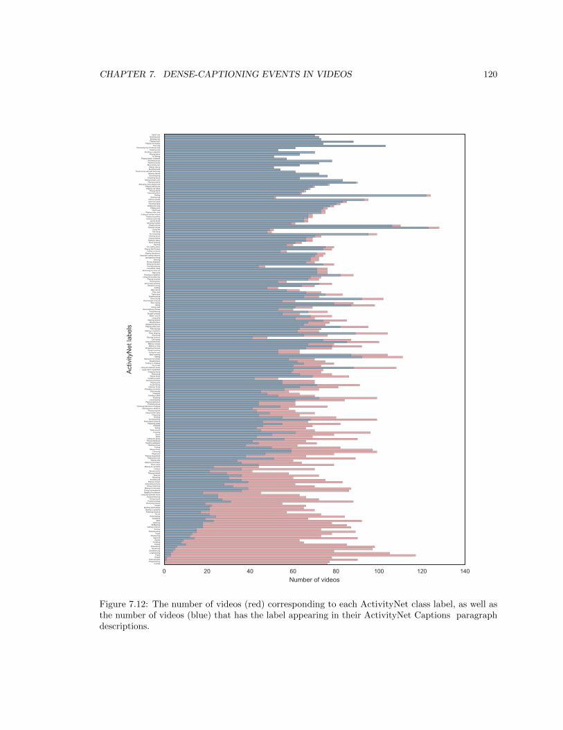
CHAPTER 7. DENSE-CAPTIONING EVENTS IN VIDEOS 120
0 20 40 60 80 100 120 140Number of videos
CumbiaPowerbockingClean and jerk
SnatchFutsal
LongboardingBreakdancing
SlackliningWaterskiing
HurlingTumbling
ZumbaCapoeira
WindsurfingTango
WakeboardingArchery
Getting a haircutBullfighting
SpinningBMX
DodgeballRollerblading
Tai chiPolishing forniture
Starting a campfireBuilding sandcastles
CricketRemoving curlers
Preparing saladFixing bicycle
Doing kickboxingUsing the pommel horse
Gargling mouthwashDoing a powerbombMaking a lemonade
Doing motocrossAssembling bicycle
Elliptical trainerShuffleboard
PlasteringShot put
Playing kickballSpread mulch
CroquetMaking an omelette
Drum corpsApplying sunscreen
Waxing skisPlaying ten pins
Playing racquetballHopscotchCanoeing
Mixing drinksCurling
Cleaning shoesHanging wallpaper
Playing blackjackCutting the grass
BalletSumo
KneelingTable soccer
SailingPaintball
Preparing pastaRock-paper-scissors
SnowboardingWelding
Ping-pongUsing uneven bars
Playing squashCarving jack-o-lanterns
Trimming branches or hedgesPolishing shoes
Playing badmintonCheerleading
KayakingDrinking coffee
VolleyballDoing karate
Changing car wheelHammer throw
Scuba divingPlaying polo
Cleaning windowsInstalling carpet
Discus throwBeer pong
Chopping woodLayup drill in basketball
Using the balance beamTug of war
Putting on makeupWashing face
Having an ice creamRafting
Baton twirlingFixing the roof
Doing crunchesWrapping presents
Making a cakeBaking cookies
Using parallel barsCalf roping
Painting furnitureSwimming
Rope skippingMaking a sandwich
Shaving legsPlaying water poloSharpening knives
Mooping floorWashing dishes
Long jumpBeach soccer
Bungee jumpingDoing fencing
Hand washing clothesDoing nails
SkiingRiver tubing
Roof shingle removalSnow tubing
SkateboardingTriple jump
Pole vaultBelly dance
KnittingPlataform diving
Doing step aerobicsDrinking beer
Playing lacrosseUsing the monkey bar
Running a marathonHigh jump
Removing ice from carHorseback ridingPeeling potatoesMowing the lawnPlaying bagpipes
ShavingSpringboard diving
Using the rowing machinePlaying saxophone
Putting on shoesPlaying field hockey
Fun sliding downPainting
Rock climbingGetting a tattooIroning clothesPainting fenceArm wrestling
Kite flyingLaying tile
Playing congasPlaying drums
Smoking hookahJavelin throw
Getting a piercingPlaying accordion
Putting in contact lensesPlaying rubik cube
Hula hoopPlaying pool
Walking the dogThrowing dartsHand car washHitting a pinata
Bathing dogSurfing
Vacuuming floorPlaying flauta
Clipping cat clawsPlaying harmonica
Swinging at the playgroundPlaying guitarra
Riding bumper carsGrooming horse
Grooming dogBlowing leaves
Tennis serve with ball bouncingBrushing teethRaking leaves
Blow-drying hairWashing handsShoveling snow
Playing beach volleyballIce fishing
Playing pianoSmoking a cigarette
Cleaning sinkDecorating the Christmas tree
Disc dogPlaying ice hockey
Playing violinBraiding hairBrushing hair
Camel ride
Act
ivity
Net
labe
ls
Figure 7.12: The number of videos (red) corresponding to each ActivityNet class label, as well asthe number of videos (blue) that has the label appearing in their ActivityNet Captions paragraphdescriptions.
Chapter 8
Conclusion
In this thesis, we have examined the research problem of leveraging large-scale visual data to study
problems in both computer vision and human-computer interaction. We began by first introducing the
Visual Genome dataset, which connects natural language to structured image concepts. Visual Genome
provides richer annotations in the forms of labeled objects, attributes, relationships, question-answer
pairs, and region descriptions than previously existing datasets. Ultimately, it is a comprehensive
dataset that is well-suited to tackle a variety of new reasoning problems in computer vision.
Next, we focused on the crowdsourcing components of constructing large-scale datasets like Visual
Genome. We highlighted the various crowdsourcing techniques employed in Visual Genome and
discussed how these techniques are transferable to the creation of new datasets. Furthermore, we
showcased a new method that produces large speedups and cost reductions in binary and categorical
labeling. We also found how crowd workers remain consistent when completing microtasks for data
collection, enabling us to determine good workers early in the process.
Finally, we demonstrated how the construction of new datasets enables us to develop techniques
to solve more complex reasoning problems. Using Visual Genome, we demonstrated early work in
a variety of new computer vision tasks, ranging from relationship prediction to generating region
descriptions. Furthermore, we built a model using a newly collected video dataset that is able to
automatically describe and temporally ground multiple sentence descriptions of any video. With the
public release of datasets like Visual Genome and ActivityNet Captions, we expect new models to
arise, allowing for greater progress in a computer’s capacity to reason about the visual world.
121
Bibliography
[1] Alexandre Alahi, Kratarth Goel, Vignesh Ramanathan, Alexandre Robicquet, Li Fei-Fei, and
Silvio Savarese. Social lstm: Human trajectory prediction in crowded spaces. In Proceedings of
the IEEE Conference on Computer Vision and Pattern Recognition, pages 961–971, 2016.
[2] Stanislaw Antol, Aishwarya Agrawal, Jiasen Lu, Margaret Mitchell, Dhruv Batra, C. Lawrence
Zitnick, and Devi Parikh. Vqa: Visual question answering. In International Conference on
Computer Vision (ICCV), 2015.
[3] Stanislaw Antol, C Lawrence Zitnick, and Devi Parikh. Zero-shot learning via visual abstraction.
In European Conference on Computer Vision, pages 401–416. Springer, 2014.
[4] Collin F. Baker, Charles J. Fillmore, and John B. Lowe. The berkeley framenet project. In
Proceedings of the 36th Annual Meeting of the Association for Computational Linguistics and
17th International Conference on Computational Linguistics - Volume 1, ACL ’98, pages 86–90,
Stroudsburg, PA, USA, 1998. Association for Computational Linguistics.
[5] Christopher Baldassano, Janice Chen, Asieh Zadbood, Jonathan W Pillow, Uri Hasson, and
Kenneth A Norman. Discovering event structure in continuous narrative perception and
memory. bioRxiv, page 081018, 2016.
[6] Debby GJ Beckers, Dimitri van der Linden, Peter GW Smulders, Michiel AJ Kompier, Marc JPM
van Veldhoven, and Nico W van Yperen. Working overtime hours: relations with fatigue, work
motivation, and the quality of work. Journal of Occupational and Environmental Medicine,
46(12):1282–1289, 2004.
[7] Michael S Bernstein, Joel Brandt, Robert C Miller, and David R Karger. Crowds in two
seconds: Enabling realtime crowd-powered interfaces. In Proceedings of the 24th annual ACM
symposium on User interface software and technology, pages 33–42. ACM, 2011.
[8] Michael S Bernstein, Greg Little, Robert C Miller, Bjorn Hartmann, Mark S Ackerman, David R
Karger, David Crowell, and Katrina Panovich. Soylent: a word processor with a crowd inside.
122
BIBLIOGRAPHY 123
In Proceedings of the 23nd annual ACM symposium on User interface software and technology,
pages 313–322. ACM, 2010.
[9] Justin Betteridge, Andrew Carlson, Sue Ann Hong, Estevam R Hruschka Jr, Edith LM Law,
Tom M Mitchell, and Sophie H Wang. Toward never ending language learning. In AAAI Spring
Symposium: Learning by Reading and Learning to Read, pages 1–2, 2009.
[10] Steven Bird. Nltk: the natural language toolkit. In Proceedings of the COLING/ACL on
Interactive presentation sessions, pages 69–72. Association for Computational Linguistics, 2006.
[11] Arijit Biswas and Devi Parikh. Simultaneous active learning of classifiers & attributes via
relative feedback. In Computer Vision and Pattern Recognition (CVPR), 2013 IEEE Conference
on, pages 644–651. IEEE, 2013.
[12] Oren Boiman and Michal Irani. Detecting irregularities in images and in video. International
journal of computer vision, 74(1):17–31, 2007.
[13] Maarten AS Boksem and Mattie Tops. Mental fatigue: costs and benefits. Brain research
reviews, 59(1):125–139, 2008.
[14] Jonathan Bragg, Mausam Daniel, and Daniel S Weld. Crowdsourcing multi-label classification
for taxonomy creation. In First AAAI conference on human computation and crowdsourcing,
2013.
[15] Steve Branson, Kristjan Eldjarn Hjorleifsson, and Pietro Perona. Active annotation translation.
In Computer Vision and Pattern Recognition (CVPR), 2014 IEEE Conference on, pages
3702–3709. IEEE, 2014.
[16] Steve Branson, Catherine Wah, Florian Schroff, Boris Babenko, Peter Welinder, Pietro Perona,
and Serge Belongie. Visual recognition with humans in the loop. In Computer Vision–ECCV
2010, pages 438–451. Springer, 2010.
[17] Jonathan Warren Brelig and Jared Morton Schrieber. System and method for automated retail
product accounting, January 30 2013. US Patent App. 13/754,664.
[18] Donald E Broadbent and Margaret HP Broadbent. From detection to identification: Response to
multiple targets in rapid serial visual presentation. Perception & psychophysics, 42(2):105–113,
1987.
[19] Jerome Bruner. Culture and human development: A new look. Human development, 33(6):344–
355, 1990.
BIBLIOGRAPHY 124
[20] Razvan C Bunescu and Raymond J Mooney. A shortest path dependency kernel for relation
extraction. In Proceedings of the conference on Human Language Technology and Empiri-
cal Methods in Natural Language Processing, pages 724–731. Association for Computational
Linguistics, 2005.
[21] Moira Burke and Robert Kraut. Using facebook after losing a job: Differential benefits of
strong and weak ties. In Proceedings of the 2013 conference on Computer supported cooperative
work, pages 1419–1430. ACM, 2013.
[22] Fabian Caba Heilbron, Victor Escorcia, Bernard Ghanem, and Juan Carlos Niebles. Activitynet:
A large-scale video benchmark for human activity understanding. In Proceedings of the IEEE
Conference on Computer Vision and Pattern Recognition, pages 961–970, 2015.
[23] Fabian Caba Heilbron, Juan Carlos Niebles, and Bernard Ghanem. Fast temporal activity
proposals for efficient detection of human actions in untrimmed videos. In Proceedings of the
IEEE Conference on Computer Vision and Pattern Recognition, pages 1914–1923, 2016.
[24] Chris Callison-Burch. Fast, cheap, and creative: evaluating translation quality using amazon’s
mechanical turk. In Proceedings of the 2009 Conference on Empirical Methods in Natural
Language Processing: Volume 1-Volume 1, pages 286–295. Association for Computational
Linguistics, 2009.
[25] Stuart K Card, Allen Newell, and Thomas P Moran. The psychology of human-computer
interaction. 1983.
[26] Dana Chandler and Adam Kapelner. Breaking monotony with meaning: Motivation in
crowdsourcing markets. Journal of Economic Behavior & Organization, 90:123–133, 2013.
[27] Jesse Chandler, Gabriele Paolacci, and Pam Mueller. Risks and rewards of crowdsourcing
marketplaces. In Handbook of human computation, pages 377–392. Springer, 2013.
[28] Angel X Chang, Manolis Savva, and Christopher D Manning. Semantic parsing for text to 3d
scene generation. ACL 2014, page 17, 2014.
[29] David L. Chen and William B. Dolan. Collecting highly parallel data for paraphrase evaluation.
In Proceedings of the 49th Annual Meeting of the Association for Computational Linguistics
(ACL-2011), Portland, OR, June 2011.
[30] Xinlei Chen, Hao Fang, Tsung-Yi Lin, Ramakrishna Vedantam, Saurabh Gupta, Piotr Dollar,
and C Lawrence Zitnick. Microsoft coco captions: Data collection and evaluation server. arXiv
preprint arXiv:1504.00325, 2015.
BIBLIOGRAPHY 125
[31] Xinlei Chen and C Lawrence Zitnick. Mind’s eye: A recurrent visual representation for image
caption generation. In Proceedings of the IEEE Conference on Computer Vision and Pattern
Recognition, pages 2422–2431, 2015.
[32] Xinlei Chen, Ashish Shrivastava, and Arpan Gupta. Neil: Extracting visual knowledge from web
data. In Computer Vision (ICCV), 2013 IEEE International Conference on, pages 1409–1416.
IEEE, 2013.
[33] Xinxiong Chen, Zhiyuan Liu, and Maosong Sun. A unified model for word sense representation
and disambiguation. In EMNLP, pages 1025–1035. Citeseer, 2014.
[34] Justin Cheng, Jaime Teevan, and Michael S Bernstein. Measuring crowdsourcing effort with
error-time curves. In Proceedings of the 33rd Annual ACM Conference on Human Factors in
Computing Systems, pages 1365–1374. ACM, 2015.
[35] Lydia B Chilton, Greg Little, Darren Edge, Daniel S Weld, and James A Landay. Cascade:
Crowdsourcing taxonomy creation. In Proceedings of the SIGCHI Conference on Human Factors
in Computing Systems, pages 1999–2008. ACM, 2013.
[36] Wongun Choi, Yu-Wei Chao, Caroline Pantofaru, and Silvio Savarese. Understanding indoor
scenes using 3d geometric phrases. In Computer Vision and Pattern Recognition (CVPR),
2013 IEEE Conference on, pages 33–40. IEEE, 2013.
[37] Lacey Colligan, Henry WW Potts, Chelsea T Finn, and Robert A Sinkin. Cognitive workload
changes for nurses transitioning from a legacy system with paper documentation to a commercial
electronic health record. International journal of medical informatics, 84(7):469–476, 2015.
[38] Aron Culotta and Jeffrey Sorensen. Dependency tree kernels for relation extraction. In
Proceedings of the 42nd Annual Meeting on Association for Computational Linguistics, page
423. Association for Computational Linguistics, 2004.
[39] Peng Dai, Jeffrey M Rzeszotarski, Praveen Paritosh, and Ed H Chi. And now for something
completely different: Improving crowdsourcing workflows with micro-diversions. In Proceedings
of the 18th ACM Conference on Computer Supported Cooperative Work & Social Computing,
pages 628–638. ACM, 2015.
[40] Marc Damashek. Gauging similarity with n-grams: Language-independent categorization of
text. Science, 267(5199):843, 1995.
[41] P. Das, C. Xu, R. F. Doell, and J. J. Corso. A thousand frames in just a few words: Lingual
description of videos through latent topics and sparse object stitching. In Proceedings of IEEE
Conference on Computer Vision and Pattern Recognition, 2013.
BIBLIOGRAPHY 126
[42] Yann Dauphin, Harm de Vries, and Yoshua Bengio. Equilibrated adaptive learning rates
for non-convex optimization. In Advances in Neural Information Processing Systems, pages
1504–1512, 2015.
[43] Jia Deng, Wei Dong, Richard Socher, Li-Jia Li, Kai Li, and Li Fei-Fei. Imagenet: A large-scale
hierarchical image database. In Computer Vision and Pattern Recognition, 2009. CVPR 2009.
IEEE Conference on, pages 248–255. IEEE, 2009.
[44] Jia Deng, Olga Russakovsky, Jonathan Krause, Michael S Bernstein, Alex Berg, and Li Fei-Fei.
Scalable multi-label annotation. In Proceedings of the SIGCHI Conference on Human Factors
in Computing Systems, pages 3099–3102. ACM, 2014.
[45] Michael Denkowski and Alon Lavie. Meteor universal: Language specific translation evaluation
for any target language. In In Proceedings of the Ninth Workshop on Statistical Machine
Translation. Citeseer, 2014.
[46] Djellel Eddine Difallah, Michele Catasta, Gianluca Demartini, and Philippe Cudre-Mauroux.
Scaling-up the crowd: Micro-task pricing schemes for worker retention and latency improvement.
In Second AAAI Conference on Human Computation and Crowdsourcing, 2014.
[47] Djellel Eddine Difallah, Michele Catasta, Gianluca Demartini, Panagiotis G Ipeirotis, and
Philippe Cudre-Mauroux. The dynamics of micro-task crowdsourcing: The case of amazon
mturk. In Proceedings of the 24th International Conference on World Wide Web, pages 617–617.
ACM, 2015.
[48] Piotr Dollar, Christian Wojek, Bernt Schiele, and Pietro Perona. Pedestrian detection: An
evaluation of the state of the art. Pattern Analysis and Machine Intelligence, IEEE Transactions
on, 34(4):743–761, 2012.
[49] Jeffrey Donahue, Lisa Anne Hendricks, Sergio Guadarrama, Marcus Rohrbach, Subhashini
Venugopalan, Kate Saenko, and Trevor Darrell. Long-term recurrent convolutional networks
for visual recognition and description. In Proceedings of the IEEE Conference on Computer
Vision and Pattern Recognition, pages 2625–2634, 2015.
[50] Steven Dow, Anand Kulkarni, Scott Klemmer, and Bjorn Hartmann. Shepherding the crowd
yields better work. In Proceedings of the ACM 2012 conference on Computer Supported
Cooperative Work, pages 1013–1022. ACM, 2012.
[51] Julie S Downs, Mandy B Holbrook, Steve Sheng, and Lorrie Faith Cranor. Are your participants
gaming the system?: screening mechanical turk workers. In Proceedings of the SIGCHI
Conference on Human Factors in Computing Systems, pages 2399–2402. ACM, 2010.
BIBLIOGRAPHY 127
[52] Olivier Duchenne, Ivan Laptev, Josef Sivic, Francis Bach, and Jean Ponce. Automatic annotation
of human actions in video. In Computer Vision, 2009 IEEE 12th International Conference on,
pages 1491–1498. IEEE, 2009.
[53] Victor Escorcia, Fabian Caba Heilbron, Juan Carlos Niebles, and Bernard Ghanem. Daps:
Deep action proposals for action understanding. In European Conference on Computer Vision,
pages 768–784. Springer, 2016.
[54] Mark Everingham, Luc Van Gool, Christopher KI Williams, John Winn, and Andrew Zisserman.
The pascal visual object classes (voc) challenge. International journal of computer vision,
88(2):303–338, 2010.
[55] Hao Fang, Saurabh Gupta, Forrest Iandola, Rupesh K Srivastava, Li Deng, Piotr Dollar,
Jianfeng Gao, Xiaodong He, Margaret Mitchell, John C Platt, et al. From captions to visual
concepts and back. In Proceedings of the IEEE Conference on Computer Vision and Pattern
Recognition, pages 1473–1482, 2015.
[56] Ali Farhadi, Mohsen Hejrati, Mohammad Amin Sadeghi, Peter Young, Cyrus Rashtchian,
Julia Hockenmaier, and David Forsyth. Every picture tells a story: Generating sentences from
images. In Computer Vision–ECCV 2010, pages 15–29. Springer, 2010.
[57] Alireza Farhadi, Ian Endres, Derek Hoiem, and David Forsyth. Describing objects by their
attributes. In Computer Vision and Pattern Recognition, 2009. CVPR 2009. IEEE Conference
on, pages 1778–1785. IEEE, 2009.
[58] Ethan Fast, Daniel Steffee, Lucy Wang, Joel R Brandt, and Michael S Bernstein. Emergent,
crowd-scale programming practice in the ide. In Proceedings of the 32nd annual ACM conference
on Human factors in computing systems, pages 2491–2500. ACM, 2014.
[59] Li Fei-Fei, Rob Fergus, and Pietro Perona. Learning generative visual models from few training
examples: An incremental bayesian approach tested on 101 object categories. Computer Vision
and Image Understanding, 106(1):59–70, 2007.
[60] Li Fei-Fei, Asha Iyer, Christof Koch, and Pietro Perona. What do we perceive in a glance of a
real-world scene? Journal of vision, 7(1):10, 2007.
[61] Vittorio Ferrari and Andrew Zisserman. Learning visual attributes. In Advances in Neural
Information Processing Systems, pages 433–440, 2007.
[62] David Ferrucci, Eric Brown, Jennifer Chu-Carroll, James Fan, David Gondek, Aditya A
Kalyanpur, Adam Lally, J William Murdock, Eric Nyberg, John Prager, et al. Building watson:
An overview of the deepqa project. AI magazine, 31(3):59–79, 2010.
BIBLIOGRAPHY 128
[63] Chaz Firestone and Brian J Scholl. Cognition does not affect perception: Evaluating the
evidence for top-down effects. Behavioral and brain sciences, pages 1–72, 2015.
[64] Kenneth D Forbus. Qualitative process theory. Artificial intelligence, 24(1):85–168, 1984.
[65] Adrien Gaidon, Zaid Harchaoui, and Cordelia Schmid. Temporal localization of actions with
actoms. IEEE transactions on pattern analysis and machine intelligence, 35(11):2782–2795,
2013.
[66] Haoyuan Gao, Junhua Mao, Jie Zhou, Zhiheng Huang, Lei Wang, and Wei Xu. Are you talking
to a machine? dataset and methods for multilingual image question. In Advances in Neural
Information Processing Systems, pages 2296–2304, 2015.
[67] Andreas Geiger, Philip Lenz, Christoph Stiller, and Raquel Urtasun. Vision meets robotics:
The kitti dataset. International Journal of Robotics Research (IJRR), 2013.
[68] Donald Geman, Stuart Geman, Neil Hallonquist, and Laurent Younes. Visual turing test for
computer vision systems. Proceedings of the National Academy of Sciences, 112(12):3618–3623,
2015.
[69] Eric Gilbert and Karrie Karahalios. Predicting tie strength with social media. In Proceedings
of the SIGCHI Conference on Human Factors in Computing Systems, pages 211–220. ACM,
2009.
[70] Ross Girshick. Fast r-cnn. In Proceedings of the IEEE International Conference on Computer
Vision, pages 1440–1448, 2015.
[71] Ross Girshick, Jeff Donahue, Trevor Darrell, and Jagannath Malik. Rich feature hierarchies
for accurate object detection and semantic segmentation. In Computer Vision and Pattern
Recognition (CVPR), 2014 IEEE Conference on, pages 580–587. IEEE, 2014.
[72] Georgia Gkioxari and Jitendra Malik. Finding action tubes. In Proceedings of the IEEE
Conference on Computer Vision and Pattern Recognition, pages 759–768, 2015.
[73] Christoph Goering, Erid Rodner, Alexander Freytag, and Joachim Denzler. Nonparametric part
transfer for fine-grained recognition. In Computer Vision and Pattern Recognition (CVPR),
2014 IEEE Conference on, pages 2489–2496. IEEE, 2014.
[74] Dan B Goldman, Brian Curless, David Salesin, and Steven M Seitz. Schematic storyboarding
for video visualization and editing. In ACM Transactions on Graphics (TOG), volume 25,
pages 862–871. ACM, 2006.
BIBLIOGRAPHY 129
[75] A. Gorban, H. Idrees, Y.-G. Jiang, A. Roshan Zamir, I. Laptev, M. Shah, and R. Sukthankar.
THUMOS challenge: Action recognition with a large number of classes. http://www.thumos.
info/, 2015.
[76] Gregory Griffin, Alex Holub, and Pietro Perona. Caltech-256 object category dataset. 2007.
[77] Zhou GuoDong, Su Jian, Zhang Jie, and Zhang Min. Exploring various knowledge in relation
extraction. In Proceedings of the 43rd annual meeting on association for computational
linguistics, pages 427–434. Association for Computational Linguistics, 2005.
[78] Abhinav Gupta and Larry S Davis. Beyond nouns: Exploiting prepositions and comparative
adjectives for learning visual classifiers. In Computer Vision–ECCV 2008, pages 16–29. Springer,
2008.
[79] Abhinav Gupta, Aniruddha Kembhavi, and Larry S Davis. Observing human-object interactions:
Using spatial and functional compatibility for recognition. Pattern Analysis and Machine
Intelligence, IEEE Transactions on, 31(10):1775–1789, 2009.
[80] Michael Gygli, Helmut Grabner, and Luc Van Gool. Video summarization by learning submod-
ular mixtures of objectives. In Proceedings of the IEEE Conference on Computer Vision and
Pattern Recognition, pages 3090–3098, 2015.
[81] Kenji Hata, Ranjay Krishna, Li Fei-Fei, and Michael S. Bernstein. A glimpse far into the future:
Understanding long-term crowd worker quality. In Proceedings of the 2017 ACM Conference
on Computer Supported Cooperative Work and Social Computing, CSCW ’17, pages 889–901,
New York, NY, USA, 2017. ACM.
[82] Patrick J. Hayes. The naive physics manifesto. Institut pour les etudes semantiques et
cognitives/Universite de Geneve, 1978.
[83] Patrick J. Hayes. The second naive physics manifesto. Theories of the Commonsense World,
pages 1–36, 1985.
[84] Marti A. Hearst, Susan T Dumais, Edgar Osman, John Platt, and Bernhard Scholkopf. Support
vector machines. Intelligent Systems and their Applications, IEEE, 13(4):18–28, 1998.
[85] Jeffrey Heer and Michael Bostock. Crowdsourcing graphical perception: using mechanical turk
to assess visualization design. In Proceedings of the SIGCHI Conference on Human Factors in
Computing Systems, pages 203–212. ACM, 2010.
[86] Robert A. Henning, Steven L Sauter, Gavriel Salvendy, and Edward F Krieg Jr. Microbreak
length, performance, and stress in a data entry task. Ergonomics, 32(7):855–864, 1989.
[87] Paul Hitlin. Research in the crowdsourcing age, a case study, July 2016.
BIBLIOGRAPHY 130
[88] Chien-Ju Ho, Aleksandrs Slivkins, Siddharth Suri, and Jennifer Wortman Vaughan. Incentivizing
high quality crowdwork. In Proceedings of the 24th International Conference on World Wide
Web, pages 419–429. ACM, 2015.
[89] Sepp Hochreiter and Jurgen Schmidhuber. Long short-term memory. Neural computation,
9(8):1735–1780, 1997.
[90] Micah Hodosh, Peter Young, and Julia Hockenmaier. Framing image description as a ranking
task: Data, models and evaluation metrics. J. Artif. Int. Res., 47(1):853–899, May 2013.
[91] Chih-Sheng Johnson Hou, Natalya F Noy, and Mark A Musen. A template-based approach
toward acquisition of logical sentences. In Intelligent Information Processing, pages 77–89.
Springer, 2002.
[92] Gary B Huang, Marwan Mattar, Tamara Berg, and Eric Learned-Miller. Labeled faces in the
wild: A database forstudying face recognition in unconstrained environments. In Workshop on
Faces in’Real-Life’Images: Detection, Alignment, and Recognition, 2008.
[93] Marius Catalin Iordan, Michelle R Greene, Diane M Beck, and Li Fei-Fei. Basic level cat-
egory structure emerges gradually across human ventral visual cortex. Journal of cognitive
neuroscience, 2015.
[94] Panagiotis G Ipeirotis. Analyzing the amazon mechanical turk marketplace. XRDS: Crossroads,
The ACM Magazine for Students, 17(2):16–21, 2010.
[95] Panagiotis G Ipeirotis, Foster Provost, and Jing Wang. Quality management on amazon
mechanical turk. In Proceedings of the ACM SIGKDD workshop on human computation, pages
64–67. ACM, 2010.
[96] Lilly C Irani and M Silberman. Turkopticon: Interrupting worker invisibility in amazon
mechanical turk. In Proceedings of the SIGCHI Conference on Human Factors in Computing
Systems, pages 611–620. ACM, 2013.
[97] Phillip Isola, Joseph J Lim, and Edward H Adelson. Discovering states and transformations in
image collections. In Proceedings of the IEEE Conference on Computer Vision and Pattern
Recognition, pages 1383–1391, 2015.
[98] Hamid Izadinia, Fereshteh Sadeghi, and Alireza Farhadi. Incorporating scene context and
object layout into appearance modeling. In Computer Vision and Pattern Recognition (CVPR),
2014 IEEE Conference on, pages 232–239. IEEE, 2014.
[99] Suyog Dutt Jain and Kristen Grauman. Predicting sufficient annotation strength for interactive
foreground segmentation. In Computer Vision (ICCV), 2013 IEEE International Conference
on, pages 1313–1320. IEEE, 2013.
BIBLIOGRAPHY 131
[100] Shuiwang Ji, Wei Xu, Ming Yang, and Kai Yu. 3d convolutional neural networks for human
action recognition. IEEE transactions on pattern analysis and machine intelligence, 35(1):221–
231, 2013.
[101] Justin Johnson, Andrej Karpathy, and Li Fei-Fei. Densecap: Fully convolutional localization
networks for dense captioning. In Proceedings of the IEEE Conference on Computer Vision
and Pattern Recognition, pages 4565–4574, 2016.
[102] Justin Johnson, Ranjay Krishna, Michael Stark, Li-Jia Li, David A Shamma, Michael Bernstein,
and Li Fei-Fei. Image retrieval using scene graphs. In IEEE Conference on Computer Vision
and Pattern Recognition (CVPR), 2015.
[103] Tatiana Josephy, Matt Lease, and Praveen Paritosh. Crowdscale 2013: Crowdsourcing at scale
workshop report. 2013.
[104] Ece Kamar, Severin Hacker, and Eric Horvitz. Combining human and machine intelligence
in large-scale crowdsourcing. In Proceedings of the 11th International Conference on Au-
tonomous Agents and Multiagent Systems-Volume 1, pages 467–474. International Foundation
for Autonomous Agents and Multiagent Systems, 2012.
[105] Adam Kapelner and Dana Chandler. Preventing satisficing in online surveys. In Proceedings of
CrowdConf, 2010.
[106] Svebor Karaman, Lorenzo Seidenari, and Alberto Del Bimbo. Fast saliency based pooling of
fisher encoded dense trajectories. In ECCV THUMOS Workshop, volume 1, 2014.
[107] David R Karger, Sewoong Oh, and Devavrat Shah. Budget-optimal crowdsourcing using
low-rank matrix approximations. In Communication, Control, and Computing (Allerton), 2011
49th Annual Allerton Conference on, pages 284–291. IEEE, 2011.
[108] David R Karger, Sewoong Oh, and Devavrat Shah. Budget-optimal task allocation for reliable
crowdsourcing systems. Operations Research, 62(1):1–24, 2014.
[109] Andrej Karpathy and Li Fei-Fei. Deep visual-semantic alignments for generating image descrip-
tions. In Proceedings of the IEEE Conference on Computer Vision and Pattern Recognition,
pages 3128–3137, 2015.
[110] Andrej Karpathy, George Toderici, Sanketh Shetty, Thomas Leung, Rahul Sukthankar, and
Li Fei-Fei. Large-scale video classification with convolutional neural networks. In Proceedings
of the IEEE conference on Computer Vision and Pattern Recognition, pages 1725–1732, 2014.
[111] Ryan Kiros, Ruslan Salakhutdinov, and Rich Zemel. Multimodal neural language models.
In Proceedings of the 31st International Conference on Machine Learning (ICML-14), pages
595–603, 2014.
BIBLIOGRAPHY 132
[112] Aniket Kittur, Ed H Chi, and Bongwon Suh. Crowdsourcing user studies with mechanical
turk. In Proceedings of the SIGCHI conference on human factors in computing systems, pages
453–456. ACM, 2008.
[113] Aniket Kittur, Jeffrey V Nickerson, Michael Bernstein, Elizabeth Gerber, Aaron Shaw, John
Zimmerman, Matt Lease, and John Horton. The future of crowd work. In Proceedings of the
2013 conference on Computer supported cooperative work, pages 1301–1318. ACM, 2013.
[114] Aniket Kittur, Boris Smus, Susheel Khamkar, and Robert E Kraut. Crowdforge: Crowdsourcing
complex work. In Proceedings of the 24th annual ACM symposium on User interface software
and technology, pages 43–52. ACM, 2011.
[115] Jonathan Krause, Justin Johnson, Ranjay Krishna, and Li Fei-Fei. A hierarchical approach
for generating descriptive image paragraphs. In Computer Vision and Patterm Recognition
(CVPR), 2017.
[116] Ranjay Krishna, Kenji Hata, Stephanie Chen, Joshua Kravitz, David A Shamma, Li Fei-Fei,
and Michael S. Bernstein. Embracing error to enable rapid crowdsourcing. In CHI’16-SIGCHI
Conference on Human Factors in Computing System, 2016.
[117] Ranjay Krishna, Kenji Hata, Frederic Ren, Li Fei-Fei, and Juan Carlos Niebles. Dense-captioning
events in videos. arXiv preprint arXiv:1705.00754, 2017.
[118] Ranjay Krishna, Yuke Zhu, Oliver Groth, Justin Johnson, Kenji Hata, Joshua Kravitz, Stephanie
Chen, Yannis Kalantidis, Li-Jia Li, David A Shamma, Michael Bernstein, and Li Fei-Fei.
Visual genome: Connecting language and vision using crowdsourced dense image annotations.
International Journal of Computer Vision, 2016.
[119] Ranjay A Krishna, Kenji Hata, Stephanie Chen, Joshua Kravitz, David A Shamma, Li Fei-Fei,
and Michael S Bernstein. Embracing error to enable rapid crowdsourcing. In Proceedings of the
2016 CHI Conference on Human Factors in Computing Systems, pages 3167–3179. ACM, 2016.
[120] Alex Krizhevsky, Ilya Sutskever, and Geoffrey E Hinton. Imagenet classification with deep
convolutional neural networks. In Advances in neural information processing systems, pages
1097–1105, 2012.
[121] Jon A Krosnick. Response strategies for coping with the cognitive demands of attitude measures
in surveys. Applied cognitive psychology, 5(3):213–236, 1991.
[122] Gerald P Krueger. Sustained work, fatigue, sleep loss and performance: A review of the issues.
Work & Stress, 3(2):129–141, 1989.
BIBLIOGRAPHY 133
[123] Hildegard Kuehne, Hueihan Jhuang, Estıbaliz Garrote, Tomaso Poggio, and Thomas Serre.
Hmdb: a large video database for human motion recognition. In Computer Vision (ICCV),
2011 IEEE International Conference on, pages 2556–2563. IEEE, 2011.
[124] Raymond Kuhn and Erik Neveu. Political journalism: New challenges, new practices. Routledge,
2013.
[125] Ranjitha Kumar, Arvind Satyanarayan, Cesar Torres, Maxine Lim, Salman Ahmad, Scott R
Klemmer, and Jerry O Talton. Webzeitgeist: design mining the web. In Proceedings of the
SIGCHI Conference on Human Factors in Computing Systems, pages 3083–3092. ACM, 2013.
[126] Christoph H Lampert, Hannes Nickisch, and Stefan Harmeling. Learning to detect unseen
object classes by between-class attribute transfer. In Computer Vision and Pattern Recognition,
2009. CVPR 2009. IEEE Conference on, pages 951–958. IEEE, 2009.
[127] Ivan Laptev, Marcin Marszalek, Cordelia Schmid, and Benjamin Rozenfeld. Learning realistic
human actions from movies. In Computer Vision and Pattern Recognition, 2008. CVPR 2008.
IEEE Conference on, pages 1–8. IEEE, 2008.
[128] Gierad Laput, Walter S Lasecki, Jason Wiese, Robert Xiao, Jeffrey P Bigham, and Chris
Harrison. Zensors: Adaptive, rapidly deployable, human-intelligent sensor feeds. In Proceedings
of the 33rd Annual ACM Conference on Human Factors in Computing Systems, pages 1935–1944.
ACM, 2015.
[129] Walter Lasecki, Christopher Miller, Adam Sadilek, Andrew Abumoussa, Donato Borrello,
Raja Kushalnagar, and Jeffrey Bigham. Real-time captioning by groups of non-experts. In
Proceedings of the 25th annual ACM symposium on User interface software and technology,
pages 23–34. ACM, 2012.
[130] Walter S Lasecki, Adam Marcus, Jeffrey M Rzeszotarski, and Jeffrey P Bigham. Using microtask
continuity to improve crowdsourcing. Technical report, Tech. rep, 2014.
[131] Walter S Lasecki, Kyle I Murray, Samuel White, Robert C Miller, and Jeffrey P Bigham. Real-
time crowd control of existing interfaces. In Proceedings of the 24th annual ACM symposium
on User interface software and technology, pages 23–32. ACM, 2011.
[132] Walter S Lasecki, Jeffrey M Rzeszotarski, Adam Marcus, and Jeffrey P Bigham. The effects of
sequence and delay on crowd work. In Proceedings of the 33rd Annual ACM Conference on
Human Factors in Computing Systems, pages 1375–1378. ACM, 2015.
[133] Edith Law, Ming Yin, Kevin Chen Joslin Goh, Michael Terry, and Krzysztof Z Gajos. Curiosity
killed the cat, but makes crowdwork better. In Proceedings of the 2016 CHI Conference on
Human Factors in Computing Systems, pages 4098–4110. ACM, 2016.
BIBLIOGRAPHY 134
[134] Claudia Leacock, George A Miller, and Martin Chodorow. Using corpus statistics and wordnet
relations for sense identification. Computational Linguistics, 24(1):147–165, 1998.
[135] Remi Lebret, Pedro O Pinheiro, and Ronan Collobert. Phrase-based image captioning. arXiv
preprint arXiv:1502.03671, 2015.
[136] David D. Lewis and Philip J. Hayes. Guest editorial. ACM Transactions on Information
Systems, 12(3):231, July 1994.
[137] Fei Fei Li, Rufin VanRullen, Christof Koch, and Pietro Perona. Rapid natural scene catego-
rization in the near absence of attention. Proceedings of the National Academy of Sciences,
99(14):9596–9601, 2002.
[138] Tao Li and Mitsunori Ogihara. Detecting emotion in music. In ISMIR, volume 3, pages 239–240,
2003.
[139] Liang Liang and Kristen Grauman. Beyond comparing image pairs: Setwise active learning
for relative attributes. In Computer Vision and Pattern Recognition (CVPR), 2014 IEEE
Conference on, pages 208–215. IEEE, 2014.
[140] Tsung-Yi Lin, Michael Maire, Serge Belongie, James Hays, Pietro Perona, Deva Ramanan, Piotr
Dollar, and C Lawrence Zitnick. Microsoft coco: Common objects in context. In Computer
Vision–ECCV 2014, pages 740–755. Springer, 2014.
[141] Greg Little. How many turkers are there, Dec 2009.
[142] Angli Liu, Stephen Soderland, Jonathan Bragg, Christopher H Lin, Xiao Ling, and Daniel S
Weld. Effective crowd annotation for relation extraction. In Proceedings of the NAACL-HLT
2016, pages 897–906. Association for Computational Linguistics, 2016.
[143] Wu Liu, Tao Mei, Yongdong Zhang, Cherry Che, and Jiebo Luo. Multi-task deep visual-
semantic embedding for video thumbnail selection. In Proceedings of the IEEE Conference on
Computer Vision and Pattern Recognition, pages 3707–3715, 2015.
[144] Cewu Lu, Ranjay Krishna, Michael Bernstein, and Li Fei-Fei. Visual relationship detection
using language priors. In European Conference on Computer Vision (ECCV). IEEE, 2016.
[145] Lin Ma, Zhengdong Lu, and Hang Li. Learning to answer questions from image using
convolutional neural network. arXiv preprint arXiv:1506.00333, 2015.
[146] Mateusz Malinowski and Mario Fritz. A multi-world approach to question answering about
real-world scenes based on uncertain input. In Advances in Neural Information Processing
Systems, pages 1682–1690, 2014.
BIBLIOGRAPHY 135
[147] Mateusz Malinowski, Marcus Rohrbach, and Mario Fritz. Ask your neurons: A neural-based
approach to answering questions about images. In Proceedings of the IEEE International
Conference on Computer Vision, pages 1–9, 2015.
[148] Tomasz Malisiewicz, Alexei Efros, et al. Recognition by association via learning per-exemplar
distances. In Computer Vision and Pattern Recognition, 2008. CVPR 2008. IEEE Conference
on, pages 1–8. IEEE, 2008.
[149] Christopher D. Manning, Mihai Surdeanu, John Bauer, Jenny Finkel, Steven J. Bethard, and
David McClosky. The Stanford CoreNLP natural language processing toolkit. In Proceedings of
52nd Annual Meeting of the Association for Computational Linguistics: System Demonstrations,
pages 55–60, 2014.
[150] Junhua Mao, Wei Xu, Yi Yang, Jiang Wang, and Alan L Yuille. Explain images with multimodal
recurrent neural networks. arXiv preprint arXiv:1410.1090, 2014.
[151] Adam Marcus and Aditya Parameswaran. Crowdsourced data management: industry and
academic perspectives. Foundations and Trends in Databases, 2015.
[152] Marcin Marsza lek, Ivan Laptev, and Cordelia Schmid. Actions in context. In IEEE Conference
on Computer Vision & Pattern Recognition, 2009.
[153] David Martin, Benjamin V Hanrahan, Jacki O’Neill, and Neha Gupta. Being a turker. In
Proceedings of the 17th ACM conference on Computer supported cooperative work & social
computing, pages 224–235. ACM, 2014.
[154] Winter Mason and Siddharth Suri. Conducting behavioral research on amazons mechanical
turk. Behavior research methods, 44(1):1–23, 2012.
[155] Winter Mason and Duncan J Watts. Financial incentives and the performance of crowds. ACM
SigKDD Explorations Newsletter, 11(2):100–108, 2010.
[156] Brian McInnis, Dan Cosley, Chaebong Nam, and Gilly Leshed. Taking a hit: Designing around
rejection, mistrust, risk, and workers experiences in amazon mechanical turk. In Proceedings of
the 2016 CHI Conference on Human Factors in Computing Systems, pages 2271–2282. ACM,
2016.
[157] Rada Mihalcea, Timothy Anatolievich Chklovski, and Adam Kilgarriff. The senseval-3 english
lexical sample task. In UNT Digital Library. Association for Computational Linguistics, 2004.
[158] Tomas Mikolov, Kai Chen, Greg Corrado, and Jeffrey Dean. Efficient estimation of word
representations in vector space. arXiv preprint arXiv:1301.3781, 2013.
BIBLIOGRAPHY 136
[159] Tomas Mikolov, Martin Karafiat, Lukas Burget, Jan Cernocky, and Sanjeev Khudanpur.
Recurrent neural network based language model. In Interspeech, volume 2, page 3, 2010.
[160] George A Miller. Wordnet: a lexical database for english. Communications of the ACM,
38(11):39–41, 1995.
[161] George A Miller and Walter G Charles. Contextual correlates of semantic similarity. Language
and cognitive processes, 6(1):1–28, 1991.
[162] Tanushree Mitra, Clayton J Hutto, and Eric Gilbert. Comparing person-and process-centric
strategies for obtaining quality data on amazon mechanical turk. In Proceedings of the 33rd
Annual ACM Conference on Human Factors in Computing Systems, pages 1345–1354. ACM,
2015.
[163] Pushmeet Kohli Nathan Silberman, Derek Hoiem and Rob Fergus. Indoor segmentation and
support inference from rgbd images. In ECCV, 2012.
[164] Allen Newell and Paul S Rosenbloom. Mechanisms of skill acquisition and the law of practice.
Cognitive skills and their acquisition, 1:1–55, 1981.
[165] Bingbing Ni, Vignesh R Paramathayalan, and Pierre Moulin. Multiple granularity analysis for
fine-grained action detection. In Proceedings of the IEEE Conference on Computer Vision and
Pattern Recognition, pages 756–763, 2014.
[166] Juan Carlos Niebles, Chih-Wei Chen, and Li Fei-Fei. Modeling temporal structure of decom-
posable motion segments for activity classification. In European conference on computer vision,
pages 392–405. Springer, 2010.
[167] Feng Niu, Ce Zhang, Christopher Re, and Jude Shavlik. Elementary: Large-scale knowledge-
base construction via machine learning and statistical inference. International Journal on
Semantic Web and Information Systems (IJSWIS), 8(3):42–73, 2012.
[168] Dan Oneata, Jakob Verbeek, and Cordelia Schmid. Efficient action localization with approxi-
mately normalized fisher vectors. In Proceedings of the IEEE Conference on Computer Vision
and Pattern Recognition, pages 2545–2552, 2014.
[169] Daniel M Oppenheimer, Tom Meyvis, and Nicolas Davidenko. Instructional manipulation
checks: Detecting satisficing to increase statistical power. Journal of Experimental Social
Psychology, 45(4):867–872, 2009.
[170] Vicente Ordonez, Girish Kulkarni, and Tamara L. Berg. Im2text: Describing images using
1 million captioned photographs. In J. Shawe-Taylor, R.S. Zemel, P.L. Bartlett, F. Pereira,
and K.Q. Weinberger, editors, Advances in Neural Information Processing Systems 24, pages
1143–1151. Curran Associates, Inc., 2011.
BIBLIOGRAPHY 137
[171] Mayu Otani, Yuta Nakashima, Esa Rahtu, Janne Heikkila, and Naokazu Yokoya. Learning
joint representations of videos and sentences with web image search. In European Conference
on Computer Vision, pages 651–667. Springer, 2016.
[172] Alok Ranjan Pal and Diganta Saha. Word sense disambiguation: a survey. arXiv preprint
arXiv:1508.01346, 2015.
[173] Yingwei Pan, Tao Mei, Ting Yao, Houqiang Li, and Yong Rui. Jointly modeling embedding and
translation to bridge video and language. In Proceedings of the IEEE Conference on Computer
Vision and Pattern Recognition, pages 4594–4602, 2016.
[174] Bo Pang and Lillian Lee. Opinion mining and sentiment analysis. Foundations and trends in
information retrieval, 2(1-2):1–135, 2008.
[175] Kishore Papineni, Salim Roukos, Todd Ward, and Wei-Jing Zhu. Bleu: a method for automatic
evaluation of machine translation. In Proceedings of the 40th annual meeting on association for
computational linguistics, pages 311–318. Association for Computational Linguistics, 2002.
[176] Amar Parkash and Devi Parikh. Attributes for classifier feedback. In Computer Vision–ECCV
2012, pages 354–368. Springer, 2012.
[177] Genevieve Patterson, Chen Xu, Hang Su, and James Hays. The sun attribute database:
Beyond categories for deeper scene understanding. International Journal of Computer Vision,
108(1-2):59–81, 2014.
[178] Mausam Daniel Peng Dai and S Weld. Decision-theoretic control of crowd-sourced workflows.
In In the 24th AAAI Conference on Artificial Intelligence (AAAI10. Citeseer, 2010.
[179] Layne P Perelli. Fatigue stressors in simulated long-duration flight. effects on performance,
information processing, subjective fatigue, and physiological cost. Technical report, DTIC
Document, 1980.
[180] Florent Perronnin, Jorge Sanchez, and Thomas Mensink. Improving the fisher kernel for
large-scale image classification. In Computer Vision–ECCV 2010, pages 143–156. Springer,
2010.
[181] Hamed Pirsiavash and Deva Ramanan. Parsing videos of actions with segmental grammars.
In Proceedings of the IEEE Conference on Computer Vision and Pattern Recognition, pages
612–619, 2014.
[182] Mary C Potter. Short-term conceptual memory for pictures. Journal of experimental psychology:
human learning and memory, 2(5):509, 1976.
BIBLIOGRAPHY 138
[183] Mary C Potter and Ellen I Levy. Recognition memory for a rapid sequence of pictures. Journal
of experimental psychology, 81(1):10, 1969.
[184] Alessandro Prest, Cordelia Schmid, and Vittorio Ferrari. Weakly supervised learning of
interactions between humans and objects. Pattern Analysis and Machine Intelligence, IEEE
Transactions on, 34(3):601–614, 2012.
[185] Vignesh Ramanathan, Congcong Li, Jia Deng, Wei Han, Zhen Li, Kunlong Gu, Yang Song,
Samy Bengio, Chuck Rossenberg, and Li Fei-Fei. Learning semantic relationships for better
action retrieval in images. In Proceedings of the IEEE Conference on Computer Vision and
Pattern Recognition, pages 1100–1109, 2015.
[186] Cyrus Rashtchian, Peter Young, Micah Hodosh, and Julia Hockenmaier. Collecting image
annotations using amazon’s mechanical turk. In Proceedings of the NAACL HLT 2010 Work-
shop on Creating Speech and Language Data with Amazon’s Mechanical Turk, pages 139–147.
Association for Computational Linguistics, 2010.
[187] Adam Reeves and George Sperling. Attention gating in short-term visual memory. Psychological
review, 93(2):180, 1986.
[188] Michaela Regneri, Marcus Rohrbach, Dominikus Wetzel, Stefan Thater, Bernt Schiele, and
Manfred Pinkal. Grounding action descriptions in videos. Transactions of the Association for
Computational Linguistics (TACL), 1:25–36, 2013.
[189] Mengye Ren, Ryan Kiros, and Richard Zemel. Image question answering: A visual semantic
embedding model and a new dataset. arXiv preprint arXiv:1505.02074, 2015.
[190] Shaoqing Ren, Kaiming He, Ross Girshick, and Jian Sun. Faster r-cnn: Towards real-time
object detection with region proposal networks. In Advances in neural information processing
systems, pages 91–99, 2015.
[191] Anna Rohrbach, Marcus Rohrbach, Wei Qiu, Annemarie Friedrich, Manfred Pinkal, and Bernt
Schiele. Coherent multi-sentence video description with variable level of detail. In German
Conference on Pattern Recognition, pages 184–195. Springer, 2014.
[192] Anna Rohrbach, Marcus Rohrbach, and Bernt Schiele. The long-short story of movie description.
In German Conference on Pattern Recognition, pages 209–221. Springer, 2015.
[193] Anna Rohrbach, Marcus Rohrbach, Niket Tandon, and Bernt Schiele. A dataset for movie
description. In Proceedings of the IEEE Conference on Computer Vision and Pattern Recognition
(CVPR), 2015.
BIBLIOGRAPHY 139
[194] Marcus Rohrbach, Sikandar Amin, Mykhaylo Andriluka, and Bernt Schiele. A database for fine
grained activity detection of cooking activities. In Computer Vision and Pattern Recognition
(CVPR), 2012 IEEE Conference on, pages 1194–1201. IEEE, 2012.
[195] Matteo Ruggero Ronchi and Pietro Perona. Describing common human visual actions in images.
In Mark W. Jones Xianghua Xie and Gary K. L. Tam, editors, Proceedings of the British
Machine Vision Conference (BMVC 2015), pages 52.1–52.12. BMVA Press, September 2015.
[196] Joel Ross, Lilly Irani, M Silberman, Andrew Zaldivar, and Bill Tomlinson. Who are the
crowdworkers?: shifting demographics in mechanical turk. In CHI’10 extended abstracts on
Human factors in computing systems, pages 2863–2872. ACM, 2010.
[197] Sascha Rothe and Hinrich Schutze. Autoextend: Extending word embeddings to embeddings
for synsets and lexemes. arXiv preprint arXiv:1507.01127, 2015.
[198] Olga Russakovsky, Jia Deng, Hao Su, Jonathan Krause, Sanjeev Satheesh, Sean Ma, Zhiheng
Huang, Andrej Karpathy, Aditya Khosla, Michael Bernstein, Alexander C. Berg, and Li Fei-Fei.
ImageNet Large Scale Visual Recognition Challenge. International Journal of Computer Vision
(IJCV), pages 1–42, April 2015.
[199] Olga Russakovsky, Jia Deng, Hao Su, Jonathan Krause, Sanjeev Satheesh, Sean Ma, Zhiheng
Huang, Andrej Karpathy, Aditya Khosla, Michael Bernstein, Alexander C Berg, and Fei-Fei Li.
Imagenet large scale visual recognition challenge. International Journal of Computer Vision,
pages 1–42, 2014.
[200] Olga Russakovsky, Li-Jia Li, and Li Fei-Fei. Best of both worlds: human-machine collaboration
for object annotation. In Proceedings of the IEEE Conference on Computer Vision and Pattern
Recognition, pages 2121–2131, 2015.
[201] Bryan C Russell, Antonio Torralba, Kevin P Murphy, and William T Freeman. Labelme: a
database and web-based tool for image annotation. International journal of computer vision,
77(1-3):157–173, 2008.
[202] Jeffrey Rzeszotarski and Aniket Kittur. Crowdscape: interactively visualizing user behavior
and output. In Proceedings of the 25th annual ACM symposium on User interface software
and technology, pages 55–62. ACM, 2012.
[203] Fereshteh Sadeghi, Santosh K Divvala, and Ali Farhadi. Viske: Visual knowledge extraction
and question answering by visual verification of relation phrases. In Proceedings of the IEEE
Conference on Computer Vision and Pattern Recognition, pages 1456–1464, 2015.
[204] Mohammad Amin Sadeghi and Ali Farhadi. Recognition using visual phrases. In Computer
Vision and Pattern Recognition (CVPR), 2011 IEEE Conference on, pages 1745–1752. IEEE,
2011.
BIBLIOGRAPHY 140
[205] Niloufar Salehi, Lilly C Irani, and Michael S Bernstein. We are dynamo: Overcoming stalling
and friction in collective action for crowd workers. In Proceedings of the 33rd Annual ACM
Conference on Human Factors in Computing Systems, pages 1621–1630. ACM, 2015.
[206] Roger C Schank and Robert P Abelson. Scripts, plans, goals, and understanding: An inquiry
into human knowledge structures. Psychology Press, 2013.
[207] Robert E Schapire and Yoram Singer. Boostexter: A boosting-based system for text catego-
rization. Machine learning, 39(2):135–168, 2000.
[208] Christian Schuldt, Ivan Laptev, and Barbara Caputo. Recognizing human actions: A local
svm approach. In Pattern Recognition, 2004. ICPR 2004. Proceedings of the 17th International
Conference on, volume 3, pages 32–36. IEEE, 2004.
[209] Karin Kipper Schuler. Verbnet: A Broad-coverage, Comprehensive Verb Lexicon. PhD thesis,
University of Pennsylvania, Philadelphia, PA, USA, 2005. AAI3179808.
[210] Sebastian Schuster, Ranjay Krishna, Angel Chang, Li Fei-Fei, and Christopher D Manning.
Generating semantically precise scene graphs from textual descriptions for improved image
retrieval. In Proceedings of the Fourth Workshop on Vision and Language, pages 70–80. Citeseer,
2015.
[211] Prem Seetharaman and Bryan Pardo. Crowdsourcing a reverberation descriptor map. In
Proceedings of the ACM International Conference on Multimedia, pages 587–596. ACM, 2014.
[212] Pierre Sermanet, David Eigen, Xiang Zhang, Michael Mathieu, Rob Fergus, and Yann LeCun.
Overfeat: Integrated recognition, localization and detection using convolutional networks. arXiv
preprint arXiv:1312.6229, 2013.
[213] Aaron D Shaw, John J Horton, and Daniel L Chen. Designing incentives for inexpert human
raters. In Proceedings of the ACM 2011 conference on Computer supported cooperative work,
pages 275–284. ACM, 2011.
[214] Victor S Sheng, Foster Provost, and Panagiotis G Ipeirotis. Get another label? improving
data quality and data mining using multiple, noisy labelers. In Proceedings of the 14th ACM
SIGKDD international conference on Knowledge discovery and data mining, pages 614–622.
ACM, 2008.
[215] Aashish Sheshadri and Matthew Lease. Square: A benchmark for research on computing crowd
consensus. In First AAAI Conference on Human Computation and Crowdsourcing, 2013.
[216] Gunnar A. Sigurdsson, Gul Varol, Xiaolong Wang, Ali Farhadi, Ivan Laptev, and Abhinav
Gupta. Hollywood in homes: Crowdsourcing data collection for activity understanding. In
European Conference on Computer Vision, 2016.
BIBLIOGRAPHY 141
[217] Herbert A Simon. Theories of bounded rationality. Decision and organization, 1(1):161–176,
1972.
[218] K. Simonyan and A. Zisserman. Very deep convolutional networks for large-scale image
recognition. CoRR, abs/1409.1556, 2014.
[219] Karen Simonyan and Andrew Zisserman. Very deep convolutional networks for large-scale
image recognition. arXiv preprint arXiv:1409.1556, 2014.
[220] Padhraic Smyth, Michael C Burl, Usama M Fayyad, and Pietro Perona. Knowledge discovery
in large image databases: Dealing with uncertainties in ground truth. In KDD Workshop,
pages 109–120, 1994.
[221] Padhraic Smyth, Usama Fayyad, Michael Burl, Pietro Perona, and Pierre Baldi. Inferring
ground truth from subjective labelling of venus images. 1995.
[222] Rion Snow, Brendan O’Connor, Daniel Jurafsky, and Andrew Y Ng. Cheap and fast—but is it
good?: evaluating non-expert annotations for natural language tasks. In Proceedings of the
conference on empirical methods in natural language processing, pages 254–263. Association for
Computational Linguistics, 2008.
[223] Richard Socher, Brody Huval, Christopher D Manning, and Andrew Y Ng. Semantic composi-
tionality through recursive matrix-vector spaces. In Proceedings of the 2012 Joint Conference
on Empirical Methods in Natural Language Processing and Computational Natural Language
Learning, pages 1201–1211. Association for Computational Linguistics, 2012.
[224] Yale Song, Jordi Vallmitjana, Amanda Stent, and Alejandro Jaimes. Tvsum: Summarizing web
videos using titles. In Proceedings of the IEEE Conference on Computer Vision and Pattern
Recognition, pages 5179–5187, 2015.
[225] Zheng Song, Qiang Chen, Zhongyang Huang, Yang Hua, and Shuicheng Yan. Contextualizing
object detection and classification. In Computer Vision and Pattern Recognition (CVPR), 2011
IEEE Conference on, pages 1585–1592. IEEE, 2011.
[226] Khurram Soomro, Amir Roshan Zamir, and Mubarak Shah. Ucf101: A dataset of 101 human
actions classes from videos in the wild. arXiv preprint arXiv:1212.0402, 2012.
[227] Alexander Sorokin and David Forsyth. Utility data annotation with amazon mechanical turk.
Urbana, 51(61):820, 2008.
[228] Andrew A Stanley, Kenji Hata, and Allison M Okamura. Closed-loop shape control of a haptic
jamming deformable surface. In Robotics and Automation (ICRA), 2016 IEEE International
Conference on, pages 2718–2724. IEEE, 2016.
BIBLIOGRAPHY 142
[229] Michael Steinbach, George Karypis, Vipin Kumar, et al. A comparison of document clustering
techniques. In KDD workshop on text mining, volume 400, pages 525–526. Boston, 2000.
[230] Hao Su, Jia Deng, and Li Fei-Fei. Crowdsourcing annotations for visual object detection. In
Workshops at the Twenty-Sixth AAAI Conference on Artificial Intelligence, 2012.
[231] Christian Szegedy, Wei Liu, Yangqing Jia, Pierre Sermanet, Scott Reed, Dragomir Anguelov,
Dumitru Erhan, Vincent Vanhoucke, and Andrew Rabinovich. Going deeper with convolutions.
In Proceedings of the IEEE Conference on Computer Vision and Pattern Recognition, pages
1–9, 2015.
[232] Omer Tamuz, Ce Liu, Serge Belongie, Ohad Shamir, and Adam Tauman Kalai. Adaptively
learning the crowd kernel. arXiv preprint arXiv:1105.1033, 2011.
[233] Bart Thomee, David A Shamma, Gerald Friedland, Benjamin Elizalde, Karl Ni, Douglas
Poland, Damian Borth, and Li-Jia Li. The new data and new challenges in multimedia research.
arXiv preprint arXiv:1503.01817, 2015.
[234] Bart Thomee, David A. Shamma, Gerald Friedland, Benjamin Elizalde, Karl Ni, Douglas
Poland, Damian Borth, and Li-Jia Li. Yfcc100m: The new data in multimedia research.
Commun. ACM, 59(2):64–73, January 2016.
[235] Bart Thomee, David A. Shamma, Gerald Friedland, Benjamin Elizalde, Karl Ni, Douglas
Poland, Damian Borth, and Li-Jia Li. Yfcc100m: The new data in multimedia research.
Communications of the ACM, 59(2), 2016. To Appear.
[236] Yicong Tian, Rahul Sukthankar, and Mubarak Shah. Spatiotemporal deformable part models
for action detection. In Proceedings of the IEEE Conference on Computer Vision and Pattern
Recognition, pages 2642–2649, 2013.
[237] Atousa Torabi, Christopher Pal, Hugo Larochelle, and Aaron Courville. Using descriptive
video services to create a large data source for video annotation research. arXiv preprint
arXiv:1503.01070, 2015.
[238] Antonio Torralba, Rob Fergus, and William T Freeman. 80 million tiny images: A large data
set for nonparametric object and scene recognition. Pattern Analysis and Machine Intelligence,
IEEE Transactions on, 30(11):1958–1970, 2008.
[239] John W Tukey. Comparing individual means in the analysis of variance. Biometrics, pages
99–114, 1949.
[240] Arash Vahdat, Bo Gao, Mani Ranjbar, and Greg Mori. A discriminative key pose sequence
model for recognizing human interactions. In Computer Vision Workshops (ICCV Workshops),
2011 IEEE International Conference on, pages 1729–1736. IEEE, 2011.
BIBLIOGRAPHY 143
[241] Manik Varma and Andrew Zisserman. A statistical approach to texture classification from
single images. International Journal of Computer Vision, 62(1-2):61–81, 2005.
[242] Ramakrishna Vedantam, C Lawrence Zitnick, and Devi Parikh. Cider: Consensus-based image
description evaluation. In Proceedings of the IEEE Conference on Computer Vision and Pattern
Recognition, pages 4566–4575, 2015.
[243] Ramakrishna Vedantam, Xiao Lin, Tanmay Batra, C Lawrence Zitnick, and Devi Parikh.
Learning common sense through visual abstraction. In Proceedings of the IEEE International
Conference on Computer Vision, pages 2542–2550, 2015.
[244] Subhashini Venugopalan, Marcus Rohrbach, Jeffrey Donahue, Raymond Mooney, Trevor Darrell,
and Kate Saenko. Sequence to sequence-video to text. In Proceedings of the IEEE International
Conference on Computer Vision, pages 4534–4542, 2015.
[245] Subhashini Venugopalan, Huijuan Xu, Jeff Donahue, Marcus Rohrbach, Raymond Mooney,
and Kate Saenko. Translating videos to natural language using deep recurrent neural networks.
arXiv preprint arXiv:1412.4729, 2014.
[246] Sudheendra Vijayanarasimhan, Prateek Jain, and Kristen Grauman. Far-sighted active learning
on a budget for image and video recognition. In Computer Vision and Pattern Recognition
(CVPR), 2010 IEEE Conference on, pages 3035–3042. IEEE, 2010.
[247] Oriol Vinyals, Alexander Toshev, Samy Bengio, and Dumitru Erhan. Show and tell: A neural
image caption generator. In Proceedings of the IEEE Conference on Computer Vision and
Pattern Recognition, pages 3156–3164, 2015.
[248] Luis Von Ahn. Games with a purpose. Computer, 39(6):92–94, 2006.
[249] Carl Vondrick, Donald Patterson, and Deva Ramanan. Efficiently scaling up crowdsourced
video annotation. International Journal of Computer Vision, 101(1):184–204, 2013.
[250] C. Wah, S. Branson, P. Welinder, P. Perona, and S. Belongie. The Caltech-UCSD Birds-200-2011
Dataset. Technical Report CNS-TR-2011-001, California Institute of Technology, 2011.
[251] Catherine Wah, Steve Branson, Pietro Perona, and Serge Belongie. Multiclass recognition
and part localization with humans in the loop. In Computer Vision (ICCV), 2011 IEEE
International Conference on, pages 2524–2531. IEEE, 2011.
[252] Catherine Wah, Grant Van Horn, Steve Branson, Subhrajyoti Maji, Pietro Perona, and Serge
Belongie. Similarity comparisons for interactive fine-grained categorization. In Computer Vision
and Pattern Recognition (CVPR), 2014 IEEE Conference on, pages 859–866. IEEE, 2014.
BIBLIOGRAPHY 144
[253] Limin Wang, Yu Qiao, and Xiaoou Tang. Action recognition and detection by combining
motion and appearance features. THUMOS14 Action Recognition Challenge, 1:2, 2014.
[254] Limin Wang, Yu Qiao, and Xiaoou Tang. Video action detection with relational dynamic-
poselets. In European Conference on Computer Vision, pages 565–580. Springer, 2014.
[255] Erich Weichselgartner and George Sperling. Dynamics of automatic and controlled visual
attention. Science, 238(4828):778–780, 1987.
[256] Peter Welinder, Steve Branson, Pietro Perona, and Serge J Belongie. The multidimensional
wisdom of crowds. In Advances in neural information processing systems, pages 2424–2432,
2010.
[257] Jacob Whitehill, Ting-fan Wu, Jacob Bergsma, Javier R Movellan, and Paul L Ruvolo. Whose
vote should count more: Optimal integration of labels from labelers of unknown expertise. In
Advances in neural information processing systems, pages 2035–2043, 2009.
[258] Jacob O Wobbrock, Jodi Forlizzi, Scott E Hudson, and Brad A Myers. Webthumb: interaction
techniques for small-screen browsers. In Proceedings of the 15th annual ACM symposium on
User interface software and technology, pages 205–208. ACM, 2002.
[259] Wayne Wolf. Key frame selection by motion analysis. In Acoustics, Speech, and Signal
Processing, 1996. ICASSP-96. Conference Proceedings., 1996 IEEE International Conference
on, volume 2, pages 1228–1231. IEEE, 1996.
[260] Stanley Wyatt, James N Langdon, et al. Fatigue and boredom in repetitive work. Industrial
Health Research Board Report. Medical Research Council, (77), 1937.
[261] Jianxiong Xiao, James Hays, Krista Ehinger, Aude Oliva, Antonio Torralba, et al. Sun database:
Large-scale scene recognition from abbey to zoo. In Computer vision and pattern recognition
(CVPR), 2010 IEEE conference on, pages 3485–3492. IEEE, 2010.
[262] Huijuan Xu, Subhashini Venugopalan, Vasili Ramanishka, Marcus Rohrbach, and Kate Saenko.
A multi-scale multiple instance video description network. arXiv preprint arXiv:1505.05914,
2015.
[263] Jun Xu, Tao Mei, Ting Yao, and Yong Rui. Msr-vtt: A large video description dataset for
bridging video and language. In Proceedings of the IEEE Conference on Computer Vision and
Pattern Recognition, pages 5288–5296, 2016.
[264] Kelvin Xu, Jimmy Ba, Ryan Kiros, Kyunghyun Cho, Aaron C. Courville, Ruslan Salakhutdinov,
Richard S. Zemel, and Yoshua Bengio. Show, attend and tell: Neural image caption generation
with visual attention. CoRR, abs/1502.03044, 2015.
BIBLIOGRAPHY 145
[265] Ran Xu, Caiming Xiong, Wei Chen, and Jason J Corso. Jointly modeling deep video and
compositional text to bridge vision and language in a unified framework. In AAAI, volume 5,
page 6, 2015.
[266] Junji Yamato, Jun Ohya, and Kenichiro Ishii. Recognizing human action in time-sequential
images using hidden markov model. In Computer Vision and Pattern Recognition, 1992.
Proceedings CVPR’92., 1992 IEEE Computer Society Conference on, pages 379–385. IEEE,
1992.
[267] Huan Yang, Baoyuan Wang, Stephen Lin, David Wipf, Minyi Guo, and Baining Guo. Unsuper-
vised extraction of video highlights via robust recurrent auto-encoders. In Proceedings of the
IEEE International Conference on Computer Vision, pages 4633–4641, 2015.
[268] Linjie Yang, Kevin Tang, Jianchao Yang, and Li-Jia Li. Dense captioning with joint inference
and visual context. arXiv preprint arXiv:1611.06949, 2016.
[269] Yi Yang, Simon Baker, Anitha Kannan, and Deva Ramanan. Recognizing proxemics in personal
photos. In Computer Vision and Pattern Recognition (CVPR), 2012 IEEE Conference on,
pages 3522–3529. IEEE, 2012.
[270] Bangpeng Yao and Li Fei-Fei. Modeling mutual context of object and human pose in human-
object interaction activities. In Computer Vision and Pattern Recognition (CVPR), 2010 IEEE
Conference on, pages 17–24. IEEE, 2010.
[271] Benjamin Yao, Xiong Yang, and Song-Chun Zhu. Introduction to a large-scale general purpose
ground truth database: methodology, annotation tool and benchmarks. In Energy Minimization
Methods in Computer Vision and Pattern Recognition, pages 169–183. Springer, 2007.
[272] Li Yao, Atousa Torabi, Kyunghyun Cho, Nicolas Ballas, Christopher Pal, Hugo Larochelle, and
Aaron Courville. Describing videos by exploiting temporal structure. In Proceedings of the
IEEE international conference on computer vision, pages 4507–4515, 2015.
[273] Ting Yao, Tao Mei, and Yong Rui. Highlight detection with pairwise deep ranking for first-
person video summarization. In Proceedings of the IEEE Conference on Computer Vision and
Pattern Recognition, pages 982–990, 2016.
[274] Serena Yeung, Alireza Fathi, and Li Fei-Fei. Videoset: Video summary evaluation through text.
arXiv preprint arXiv:1406.5824, 2014.
[275] Peter Young, Alice Lai, Micah Hodosh, and Julia Hockenmaier. From image descriptions
to visual denotations: New similarity metrics for semantic inference over event descriptions.
Transactions of the Association for Computational Linguistics, 2:67–78, 2014.
BIBLIOGRAPHY 146
[276] Haonan Yu, Jiang Wang, Zhiheng Huang, Yi Yang, and Wei Xu. Video paragraph captioning
using hierarchical recurrent neural networks. In Proceedings of the IEEE Conference on
Computer Vision and Pattern Recognition, pages 4584–4593, 2016.
[277] Licheng Yu, Eunbyung Park, Alexander C. Berg, and Tamara L. Berg. Visual Madlibs: Fill in
the blank Image Generation and Question Answering. arXiv preprint arXiv:1506.00278, 2015.
[278] Daojian Zeng, Kang Liu, Siwei Lai, Guangyou Zhou, and Jun Zhao. Relation classification via
convolutional deep neural network. In Proceedings of COLING, pages 2335–2344, 2014.
[279] Hong Jiang Zhang, Jianhua Wu, Di Zhong, and Stephen W Smoliar. An integrated system for
content-based video retrieval and browsing. Pattern recognition, 30(4):643–658, 1997.
[280] Dengyong Zhou, Sumit Basu, Yi Mao, and John C Platt. Learning from the wisdom of crowds
by minimax entropy. In Advances in Neural Information Processing Systems, pages 2195–2203,
2012.
[281] GuoDong Zhou, Min Zhang, Dong Hong Ji, and Qiaoming Zhu. Tree kernel-based relation
extraction with context-sensitive structured parse tree information. EMNLP-CoNLL 2007,
page 728, 2007.
[282] Jun Zhu, Zaiqing Nie, Xiaojiang Liu, Bo Zhang, and Ji-Rong Wen. Statsnowball: a statistical
approach to extracting entity relationships. In Proceedings of the 18th international conference
on World wide web, pages 101–110. ACM, 2009.
[283] Yuke Zhu, Alireza Fathi, and Li Fei-Fei. Reasoning about Object Affordances in a Knowledge
Base Representation. In European Conference on Computer Vision, 2014.
[284] Yuke Zhu, Ce Zhang, Christopher Re, and Li Fei-Fei. Building a Large-scale Multimodal
Knowledge Base System for Answering Visual Queries. In arXiv preprint arXiv:1507.05670,
2015.
[285] C Lawrence Zitnick and Devi Parikh. Bringing semantics into focus using visual abstraction.
In Computer Vision and Pattern Recognition (CVPR), 2013 IEEE Conference on, pages
3009–3016. IEEE, 2013.
Related Documents