Master of Engineering in Electrical Engineering and ...

Efficient Coordinate Descent for Ranking with Domination Loss

Mark A. Stevens

S.B. EECS, M.I.T., 2009

Submitted to the Department of Electrical Engineering and Computer Science

in Partial Fulfillment of the Requirements for the Degree of

Master of Engineering in Electrical Engineering and Computer Science

at the Massachusetts Institute of Technology MASSACHUSEiTESS IUTEOF TECHN0-1..OGY

May, 2010 -

@2010 Massachusetts Institute of Technology AUG 2 4 2010All rights reserved LI A E

LIBRARIES

Author

Department of Electrical Engineering and Computer Science

May 17, 2010

Certified By's/i

Yoram Singer, Google Research

VI-A Company Thesis Supervisor

Certified By

Professor Michael Collins

M.I.T. Thesis Supervisor

Accepted By

Dr. Christopher J. Terman

Chairman, Department Committee on Graduate Theses

, , e n -

Abstract. We define a new batch coordinate-descent ranking algorithm based on a domination loss,

which is designed to rank a small number of positive examples above all negatives, with a large penalty on

false positives. Its objective is to learn a linear ranking function for a query with labeled training examples in

order to rank documents. The derived single-coordinate updates scale linearly with respect to the number of

examples. We investigate a number of modifications to the basic algorithm, including regularization, layers

of examples, and feature induction.

The algorithm is tested on multiple datasets and problem settings, including Microsoft's LETOR dataset,

the Corel image dataset, a Google image dataset, and Reuters RCV1. Specific results vary by problem

and dataset, but the algorithm generally performed similarly to existing algorithms when rated by average

precision and precision at top k. It does not train as quickly as online algorithms, but offers extensions

to multiple layers, and perhaps most importantly, can be used to produce extremely sparse weight vectors.

When trained with feature induction, it achieves similarly competitive performance but with much more

compact models.

1 Introduction

Ranking is the task of ordering a set of inputs according to how well they match some label (or set of labels).

The learning task is to find a function F(x), where for some set of inputs x, F(xi) > F(xj) if and only if

xi should be ranked above xj. Such a ranking function can be used in a wide variety of applications, from

improving upon the results of other learning problems (reranking another algorithm's output) to finding the

best matches between complex inputs like images and a given label. The output from ranking may be used

in a variety of ways - the total ordering may be useful or the selection of the highest-ranked elements may

be useful. Lebanon and Lafferty show that ranking algorithms may be used as input to ensemble classifiers

[9] and find that such ensembles are competitive with those based on traditional classifiers.

Ranking methods are commonly developed by modifying traditional classifiers to output a ranking func-

tion F(x), where the output of F(x) is roughly analagous to the distance (margin) between an input and

a decision boundary in the original classification problem. In such a classifier, points with a larger margin

are classified with a greater confidence than those with smaller margins and could be ranked higher. For

instance, Grangier et al's PAMIR method for ranking image-label matches is loosely based on classification

with SVMs and the kernel trick. [7] In the most general case, training instances may be labeled according

to a directed graph, where each edge in the graph indicates that its starting vertex should be ranked above

its terminal vertex, with no assumptions that the graph is acyclic or the ranking preferences consistent. In

practice, most existing ranking algorithms assume one set of positive examples and one set of negatives.

While our algorithm does not efficiently compute the most general case, it does extend to cover training

instances that are ordered consistently, i.e. those where the "ranked above" relationship is transitive.

Much prior work has been done on ranking problems. Grangier et al [7] introduced a ranking method used

to retrieve images based on input text queries. Their method, Passive-Aggressive model for Image Retrieval

(PAMIR) was adapted from kernel-based classifiers. This method exceeds other retreival techniques in

experiments with the Corel dataset. One of the strengths of this algorithm is that it does not rely on an

intermediate tagging of images with contained concepts, but instead trains directly for ranking performance

- a benefit which the new ranking algorithm shares. PAMIR's ranking function F is based on text retrieval,

and sets F(q, p) = q - f(p), where q is the query, p is a picture, and f(p) is a mapping from the image space

to the text space; finding this function is the learning problem solved by PAMIR. Much like an SVM, the

method first redefines F(q, p) = E qtwt - (p), so that wt defines a hyperplane separator learned for each

query term t with some weight qt. They also recast the problem with kernels. w is then calculated using the

Passive-Aggressive algorithm to minimize the hinge loss L(w) = E Y,- max(O, 1 - w -qtp++ w -qtp-). By

combining models for different queries, they were able to provide rankings for queries which were not directly

trained on. One major advantage of this approach is that the algorithm is online - training examples are

randomly drawn, which leads to extremely fast training.

Elisseeff and Weston [6] also developed a SVM-based label ranking learning system. Noting past research

showing the merit of controlling model complexity, they use an all-pairs approach to develop a large-margin

ranker. Their loss function is based on the average fraction of misordered pairs, and they use regularization

to reduce overfitting.

Shashua and Levin developed another SVM-based ranking system and investigated separating instances

into classes, with margin between each class, similarly to how we define the multiple layer ranking problem

in Sec. 3. Whereas they try two methods for the margin, e.g. maximizing either the smallest margin or the

sum of margins, the Domination Rank does both, with more focus on the smaller margin at any step.

Whereas most ranking methods minimize a surrogate loss function rather than maximizing some actual

performance measure, Xu and Li introduced a ranking method called AdaRank [8] directly based on per-

formance measures NDCG (Normalized Discounted Cumulative Gain) and MAP (Mean Average Precision).

Their algorithm is similar to AdaBoost, in that at each step t they select a weak ranker ht (like the weak

classifier in AdaBoost) based on its performance against the most influential training instances, as deter-

mined by the performance measure, instead of some margin. It is designed for the query - multiple document

structure used in the Learning To Rank dataset, LETOR, which we use in experiments in Sec. 8.1.

Cao et al [15] introduce a ranking algorithm ListNet based again on the LETOR structure, where inputs

are in the form of a list, which allows them to avoid the slow all-pairs formulation of ranking problems -

their learning objective is to reproduce this list ordering. This formulation is similar to the transitive layers

we will use for multilayer domination rank. They use Neural Networks as the actual learning method. We

compare Domination Rank to both ListNet and AdaRank (among other algorithms), and find that it often

exceeds these, despite not being targeted to the LETOR dataset as these are.

Schapire and Singer [11] investigated using ranking to solve a multiclass, multiple label problem. In this

setting, correct labels should be ranked above incorrect labels. Their algorithm, called AdaBoost.MR, trained

a ranker given a set of correct labels and incorrect labels, with errors occuring only when f(x, 11) < f(x, lo),

where 11 was a correct label and lo an incorrect one. Freund et al (2003) [14] introduced an algorithm called

RankBoost which was also used to apply the AdaBoost algorithm to ranking. This method outperformed

regression and nearest neighbors for the task of ranking movie preferences. Its loss and updates were similar

to those used in Collins (2000) [41 and Schapire and Singer (1999) [11]. RankBoost is also included in the

LETOR experiments in Sec. 8.1.

Collins (2000, 2002) [3, 4} applied this boosting-based ranker to the problem of reranking outputs from a

probabilistic method to improve the selection of a best match. Their algorithm reranked the output of a prob-

abilistic text parser in order to achieve greater accuracy than the parser alone. They investigate two loss func-

tions for ranking, LogLoss = EZ log (1 + Zji 2 eF(i=F(i,1)) and ExpLoss = Ej Z7- 2 eF(zi,)-F(zi,1)

Both maximize the margin between the best parsing (a single human-verified correct sentence parsing) and

all others.

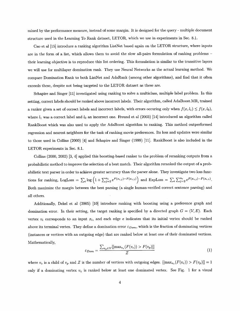
Additionally, Dekel et al (2005) [10] introduce ranking with boosting using a preference graph and

domination error. In their setting, the target ranking is specified by a directed graph G = (V, E). Each

vertex v corresponds to an input xi, and each edge e indicates that its initial vertex should be ranked

above its terminal vertex. They define a domination error eDom, which is the fraction of dominating vertices

(instances or vertices with an outgoing edge) that are ranked below at least one of their dominated vertices.

Mathematically,

EDom - vpEv [[maxvc(F(ve)) > F(v,)]]

where v is a child of vp and Z is the number of vertices with outgoing edges. [[maxv, (F(ve)) > F(v,)]] = 1

only if a dominating vertex vc is ranked below at least one dominated vertex. See Fig. 1 for a visual

24 5

2 3

1 2

5 4

Figure 1: Given a graph of desired labels and rankings 1 > 2 > 3 > 4 > 5, the subgraphs Gk on theright correspond to partitioning the graph to calculate the domination loss. Here, the domination errorEDom = 2/5, since the two graphs on the right are not satisfied.

explanation of the domination error.

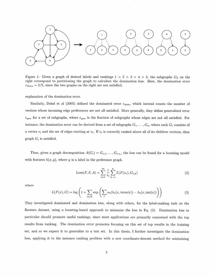
Similarly, Dekel et al (2005) defined the dominated error Edom, which instead counts the number of

vertices whose incoming edge preferences are not all satisfied. More generally, they define generalized error

Egen for a set of subgraphs, where cgen is the fraction of subgraphs whose edges are not all satisfied. For

instance, the domination error can be derived from a set of subgraphs G1 ,..., Ga, where each Gi consists of

a vertex vi and the set of edges starting at vi. If vi is correctly ranked above all of its children vertices, then

graph Gi is satisfied.

Then, given a graph decomposition A(Gj) = Gj,1,..., Gis, , the loss can be found for a boosting model

with features h(x, y), where y is a label in the preference graph.

Loss(F, S, A) = E - L(F(xi), Gj,k) (2)i=1 k=1

where

L(F(x), G) = log + E exp ( at (ht (x, term(e)) - ht (x, init(e)) (3)\ eE E \t//

They investigated dominated and domination loss, along with others, for the label-ranking task on the

Reuters dataset, using a boosting-based approach to minimize the loss in Eq. (3). Domination loss in

particular should promote useful rankings, since most applications are primarily concerned with the top

results from ranking. The domination error promotes focusing on this set of top results in the training

set, and so we expect it to generalize to a test set. In this thesis, I further investigate the domination

loss, applying it to the instance ranking problem with a new coordinate-descent method for minimizing

domination loss.

2 Basic Ranking with Domination Loss

Vectors are denoted in bold face, e.g, x, and are assumed to be in column orientation. The transpose of

a vector is denoted xt and is thus a row vector. The (vector) expectation of a set of vectors {xi} with

respect to a discrete distribution p is denoted, E,[x] = j p3 xo. We are given a set of instances (images)

per query which are represented as vectors in R". The ith image for query q, denoted Xq,i, is associated

with a quality feedback, denoted rq,i. Given groupings of images into queries with their feedback we wish

to learn a ranking, and not a classification function, f : R' - R. Concretely, we would like the function f

to induce an ordering such that f(xq,i) > f(xq,j) -> rq,i > rq,j. We use the domination loss as a surrogate

convex loss function to promote the ordering requirement. For an instance Xq,i we denote by D(q, i) the set

of instances that should be ranked below it according to the feedback,

D(q, i) = {jIrq,i > rq,j} . (4)

The combinatorial domination loss is one if there exists j E D(q, i) such that f(xq,j) > f(xq,i), that is, the

requirement that the ith instance dominates all the instances in D(q, i) is violated at least once. Note this

implies a large effect from false positives.

We would like to optimize this loss function via coordinate descent, so we need a convex approximation

to it. The convex relaxation we use for each dominating instance xq,i is,

£D(Xq,i; f) = log 1 + 1 ef(j-f (xq)A(,i,) (5)jED(q,i)

where A(q, i, j) c R+ is a margin requirement between the scores of the ith and the jth instances. See

Section 5 for a discussion of adding a regularization term.

For now, we focus on a special case in which rq,i E {-1,+1}, that is, each instance is either positive

(good, relevant) or negative (bad, irrelevant). Later on we discuss a few generalizations. In this case, the

set {j s.t. ]i : Xq,j D(q, i)} simply amounts to {jjrqj = -1}, which does not depend on the index i and

thus we overload notation and denote it as D(q). For simplicity we assume that A(q, i, j) = 0 and discuss

relaxations of this assumption below. We further assume that f is a linear function, f(x) = w - x. The

empirical loss with respect to w for a set of queries, instances, and their feedback is,

LD(w) = s log 1+ 1 eWd(Xa -Xso) (6)q,i jEEv(q,i)

For brevity and simplicity we drop the dependency on the query index q, focus on a single domination-loss

term, £D (xi; w), and perform simple algebraic manipulations,

-D(xi; W) =log ( iEfj~ewx)= log ' -w 'x , (7)

where D(i) = D(i) U {i}.

In order to minimize this loss term, we would like to select a series of minimizing updates to the weight

w. To do so, we will upper bound the true loss function with a Taylor expansion at each step, and then

select the update that minimizes that upper bound. Specifically, we would like to construct a quadratic

upper bound that may be minimized easily. Let us first compute the gradient and Hessian of fD(xj; w) with

respect to w so that we may construct this upper bound. Taking the first order derivatives with respect to

the components of w we get,

Vw ED(Xi; w) = _jE() e.x - = E,,[X] - z ,ZieD(i) ew - ]

where pi is the empirical distribution whose r'h component is p_ = ewx- /Z and Z is a normalization constant

ZjEfe(') . Thus,ePr'

Pr=Zj~f(i) ewxi

Taking the second order derivatives while using the same convention above we get that the Hessian computed

at w is,

Hi(w) = V2 £D(x,; w) = E, [xxt] - E, [x] (Ep, [x])f

Using the mean value theorem, the loss for a single query at w + 6 can now be written as,

£D(xi;w+ 6 ) = Ev(xi;w)+VW.6+ 6t Hi(w+a6)62= £-D(Xi;w)+(Epfx] - X).6+ I Ep [(6.X)2] (.- ~i[]

where Ji is the empirical distribution induced by w + ab for some a c [0, 1].

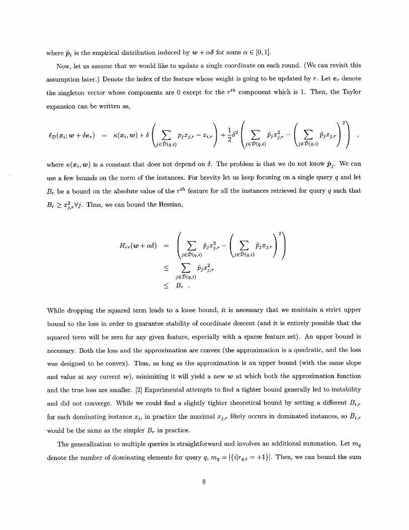
Now, let us assume that we would like to update a single coordinate on each round. (We can revisit this

assumption later.) Denote the index of the feature whose weight is going to be updated by r. Let er denote

the singleton vector whose components are 0 except for the rth component which is 1. Then, the Taylor

expansion can be written as,

2

e-D(Xi; w ± er) K(Xi, w) ±6 ( i PjXj,r -Xi~r)+ ±162 pjXj2r (Z ij~r 2)~

(iE D(q, i) 2 jEb)(q,i) (jEn(q,i) )

where x(xi, w) is a constant that does not depend on 6. The problem is that we do not know Pi. We can

use a few bounds on the norm of the instances. For brevity let us keep focusing on a single query q and let

Br be a bound on the absolute value of the r'h feature for all the instances retrieved for query q such that

Br > X2,,Vj. Thus, we can bound the Hessian,

2

Hrr (W + aJ) =2 i ,- jx~

(jEf)(q,i) (jEfb(q,i)

YZ Pj%,r

jet'(q,i)

< Br

While dropping the squared term leads to a loose bound, it is necessary that we maintain a strict upper

bound to the loss in order to guarantee stability of coordinate descent (and it is entirely possible that the

squared term will be zero for any given feature, especially with a sparse feature set). An upper bound is

necessary. Both the loss and the approximation are convex (the approximation is a quadratic, and the loss

was designed to be convex). Thus, as long as the approximation is an upper bound (with the same slope

and value at any current w), minimizing it will yield a new w at which both the approximation function

and the true loss are smaller. [2] Experimental attempts to find a tighter bound generally led to instability

and did not converge. While we could find a slightly tighter theoretical bound by setting a different Bi,r

for each dominating instance xi, in practice the maximal Xj,r likely occurs in dominated instances, so Bi,r

would be the same as the simpler Br in practice.

The generalization to multiple queries is straightforward and involves an additional summation. Let mq

denote the number of dominating elements for query q, mq = I{ilrq,i = +1}|. Then, we can bound the sum

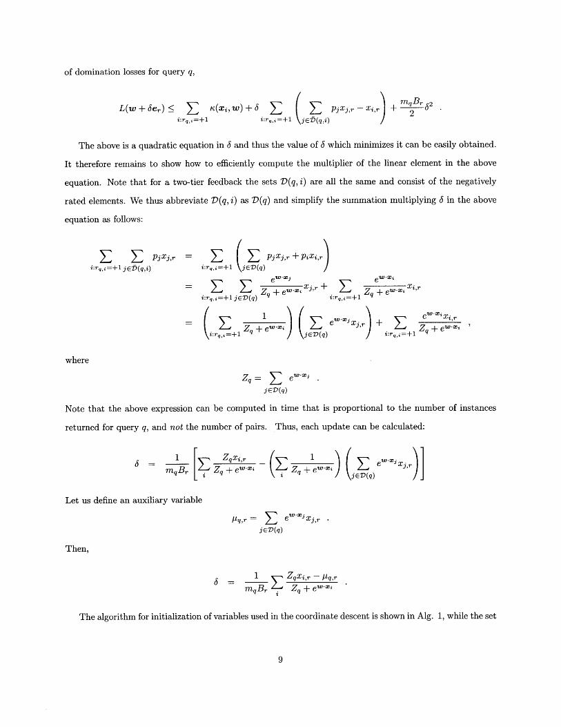
of domination losses for query q,

L(w+Jer) < i'(x,w)+6 5 ( pjxj,r xir)+ mqBr6 2

i:rg,i=+1 i:rg,i=+1 kjE)D(q,i)

The above is a quadratic equation in J and thus the value of 6 which minimizes it can be easily obtained.

It therefore remains to show how to efficiently compute the multiplier of the linear element in the above

equation. Note that for a two-tier feedback the sets D(q, i) are all the same and consist of the negatively

rated elements. We thus abbreviate D(q, i) as D(q) and simplify the summation multiplying 6 in the above

equation as follows:

E E PjXj, = Ei:r,i=+l jEU(q,i) i:rq,i=+l

i:rg,i=+1

( 1:pjxj,r + pixi,rjED)(q)

ew-xj ew-xi

Zq + ew-x Zq + e r * 'jED(q) i:rg,i=+1

ew x Xj,r + Zq +ew Xii:rg,i=+1

where

Zq 5 e***a2

jED(q)

Note that the above expression can be computed in time that is proportional to the number of instances

returned for query q, and not the number of pairs. Thus, each update can be calculated:

myB_ E ZqXir e** _,+e -_

6=mq~R [ Zq ± ew~xi (Sq+ ewx

Let us define an auxiliary variable

lq,r 5 Y ew*'xixj,rjED(q)

Then,

I - Zgxi,r - pq,r

mqBr 5 Zq+e***

The algorithm for initialization of variables used in the coordinate descent is shown in Alg. 1, while the set

Zq + e*'*i Yi: r., i=+1 ) jiED (q)

( ED(q)

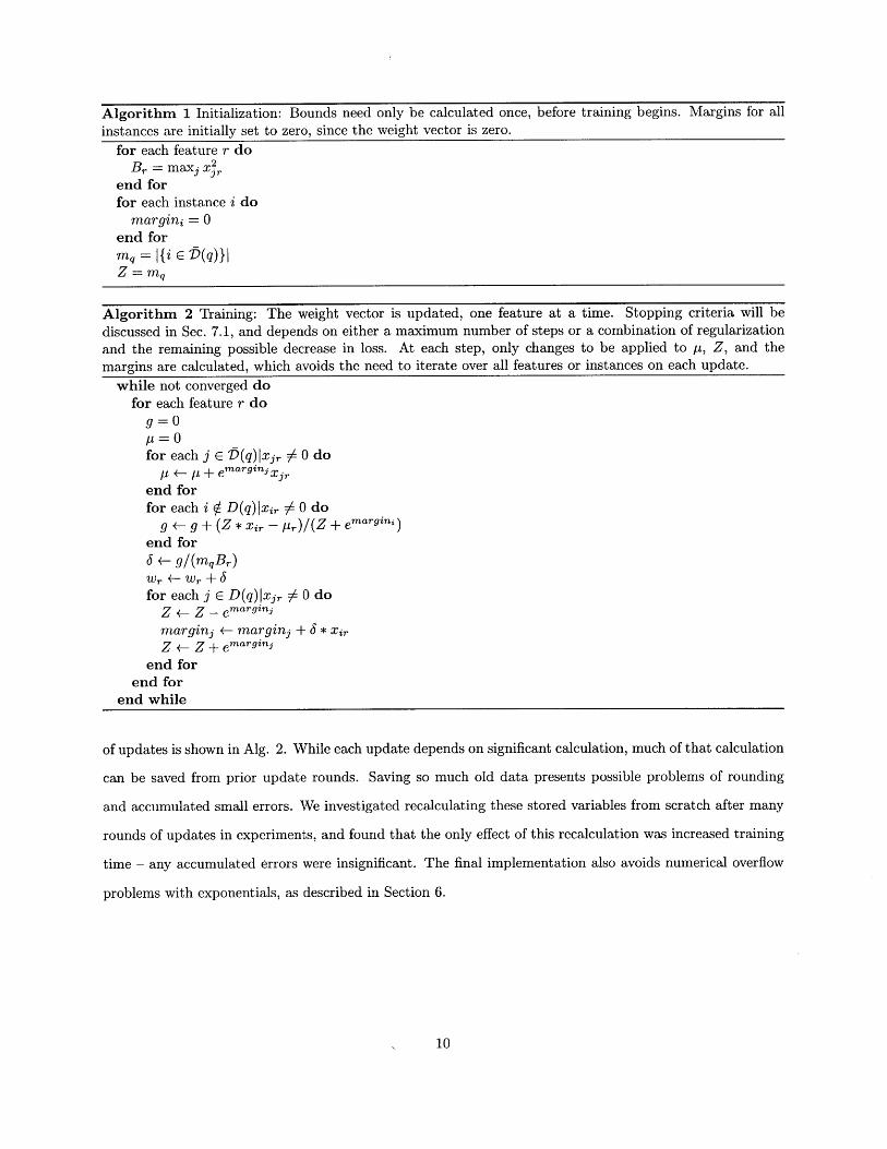
Algorithm 1 Initialization: Bounds need only be calculated once, before training begins. Margins for allinstances are initially set to zero, since the weight vector is zero.

for each feature r doBr = maxj X

end forfor each instance i do

margini = 0end formq =Ili E D(g)}|Z = mq

Algorithm 2 Training: The weight vector is updated, one feature at a time. Stopping criteria will bediscussed in Sec. 7.1, and depends on either a maximum number of steps or a combination of regularizationand the remaining possible decrease in loss. At each step, only changes to be applied to I, Z, and themargins are calculated, which avoids the need to iterate over all features or instances on each update.

while not converged dofor each feature r do

g =0/= 0for each j E D(q)Ixjr # 0 do

P 4- A + e marginj Xjr

end forfor each i V D(q)lxir $ 0 do

g +- g + (Z * Xir - pr)/(Z + emargini)end for6 +- g/(mqBr)Wr +- Wr + 6for each j E D(q)|xjr / 0 do

Z <- Z - e marginj

margin, <- marginj + 6 * xir

Z <- Z + e marginj

end forend for

end while

of updates is shown in Alg. 2. While each update depends on significant calculation, much of that calculation

can be saved from prior update rounds. Saving so much old data presents possible problems of rounding

and accumulated small errors. We investigated recalculating these stored variables from scratch after many

rounds of updates in experiments, and found that the only effect of this recalculation was increased training

time - any accumulated errors were insignificant. The final implementation also avoids numerical overflow

problems with exponentials, as described in Section 6.

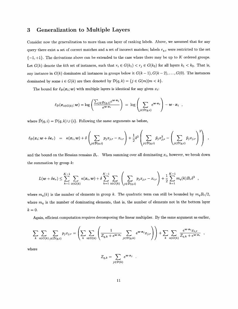
3 Generalization to Multiple Layers

Consider now the generalization to more than one layer of ranking labels. Above, we assumed that for any

query there exist a set of correct matches and a set of incorect matches; labels rq,i were restricted to the set

{-1, + 1}. The derivations above can be extended to the case where there may be up to K ordered groups.

Let G(k) denote the kth set of instances, such that ri E G(k 1 ) < rj E G(k 2 ) for all layers ki < k2 . That is,

any instance in G(k) dominates all instances in groups below it G(k - 1), G(k - 2),..., G(O). The instances

dominated by some i E G(k) are then denoted by D(q, k) = {j E G(m)Im < k}.

The bound for £-D(xi; w) with multiple layers is identical for any given xi:

£D(XiEG(k); w) = log ( jEb(qi)ewX) log wX -

\jef(q,i)

where D(q, i) = D(q, k) U { i}. Following the same arguments as before,

jE(q,i) jED(q,i)

2

(jEn(q,i) )and the bound on the Hessian remains Br. When summing over all dominating xi, however, we break down

the summation by group k:

K-1 K-1

L(w + ±er) <.5 E(xi,w ) + 6 E Ek=1 iGG(k) k=1 iEG(k)

1K-1 6pjxj,r - xi,r + ( EK mq(k)Br32

j E D(q,i) k=1

where mq(k) is the number of elements in group k. The quadratic term can still be bounded by mqBr/ 2 ,

where mq is the number of dominating elements, that is, the number of elements not in the bottom layer

k = 0.

Again, efficient computation requires decomposing the linear multiplier. By the same argument as earlier,

PjXj,r = 5 r Zk ex1 ew ZXj3 ± zwXirk iEG(k) jE-(q,i) k iEG(k) jED(q,k) k iEG(k)

where

Zq,k = 5 e*'x

jGD(k)

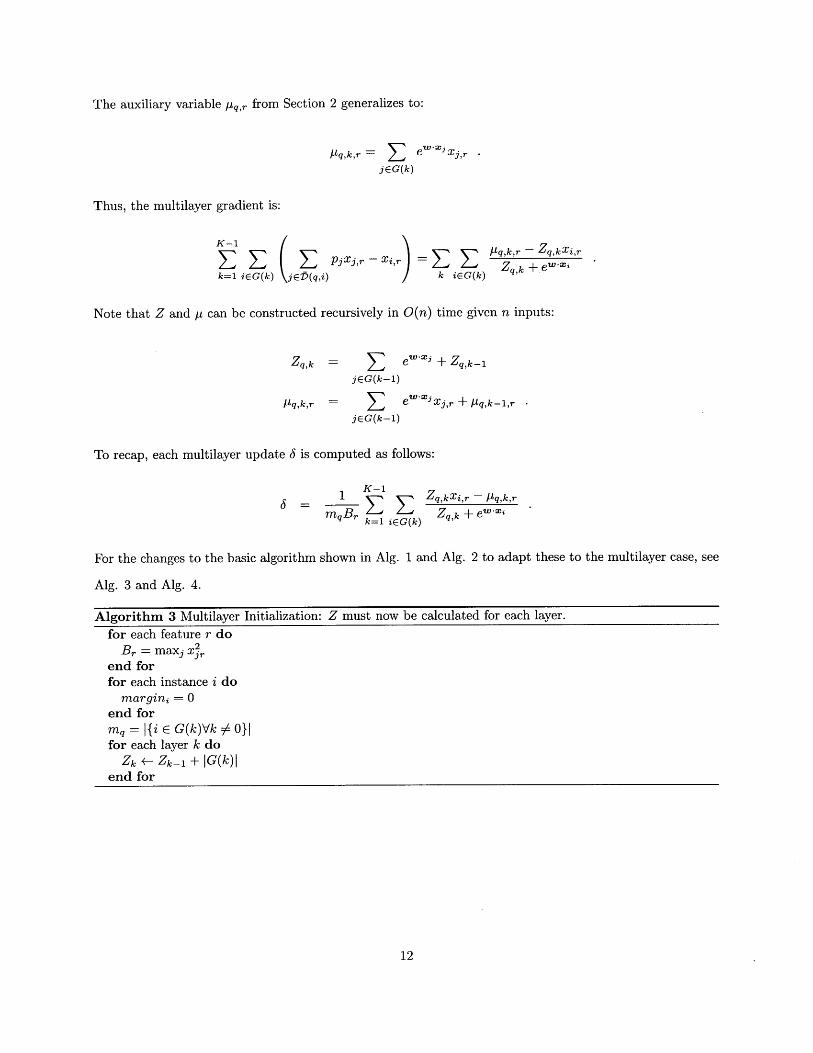
The auxiliary variable [Lq,r from Section 2 generalizes to:

[Lqkr = Gk ew) xjrjEG(k)

Thus, the multilayer gradient is:

K-1

k=1 :i E ' , - GrGkk=1 iEG(k) (jEt(q,i) / k iEG(k)

/Iq,k,r - Zq,kXi,r

Zq,k ± ewxi

Note that Z and p can be constructed recursively in O(n) time given n inputs:

Zq,k = 1:jEG(k-1)

pq,k,r = EjEG(k-1)

eW' + Zq,k-1

ew*xXj,r - /,k-1,r

To recap, each multilayer update 6 is computed as follows:

_ I K-1 Zq,kxi,r -- pq,k,r

~E mq: Zq~ e"'* 'mqBr k=1 iEG(k)

For the changes to the basic algorithm shown in Alg. 1 and Alg. 2 to adapt these to the multilayer case, see

Alg. 3 and Alg. 4.

Algorithm 3 Multilayer Initialization: Z must nowfor each feature r do

2Br = maxj xjr

end forfor each instance i do

margini = 0

end formg {i E G(k)Vk #0}|for each layer k do

Zk <- Zk- + IG(k)Iend for

be calculated for each layer.

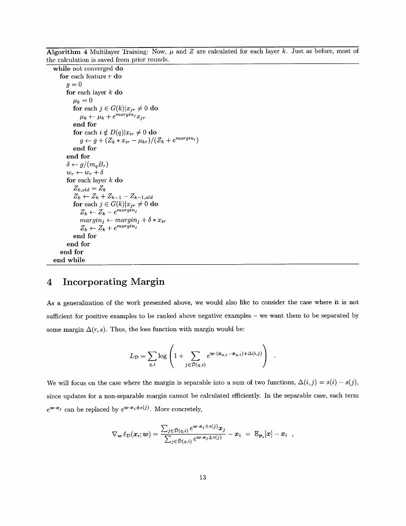
Algorithm 4 Multilayer Training: Now, y and Z are calculated for each layer k. Just as before, most ofthe calculation is saved from prior rounds.

while not converged dofor each feature r do

g = 0for each layer k do

yk = 0for each j E G(k)Ixjr f 0 do

Pk <- Pk + emargini3 >end forfor each i V D(q)Ixir # 0 do

g +- g + (Zk * Xir - pr)/(Zk+ emarini)end for

end for6 +- g/(mqBr)

Wr <- Wr + 6for each layer k do

Zk,0 id = Zk

Zk <- Zk + Zk_1 - Zk l,oldfor each j C G(k)Ixjr / 0 do

Zk +- Zk - emargini

margin3 +- marginj + 6 * xi,

Zk +- Zk - emargini

end forend for

end forend while

4 Incorporating Margin

As a generalization of the work presented above, we would also like to consider the case where it is not

sufficient for positive examples to be ranked above negative examples - we want them to be separated by

some margin A(r, s). Thus, the loss function with margin would be:

LoD=Elog 1+ E eW-(Xmerme)+i' j).q,L je'(q,i)

We will focus on the case where the margin is separable into a sum of two functions, A(i, j) = s(i) - s(j),

since updates for a non-separable margin cannot be calculated efficiently. In the separable case, each term

ewxi" can be replaced by ewx Ws(j). More concretely,

Ve vD(Xi; W) = ZjED(q) ew-os s(j)xj -i = E,,[X] - zi

ZjEf(q,i) ewxa±s(i) - =E.~-~

Algorithm 5 Initialization for Margins

for each instance i domargini = s(i)

end for

where probability is now defined

Given this new definition for p,

case, and yields updates

ew-x,ks(r)Pr E (q,i) ew-os s(j)

the rest of the derivation is identical to that for the original zero-margin

6= Z E Pq exi)mqB, iZg + ew-xi+s i)'

where

plq,r = . ewxis(i)xjrjED(q,k)

Zq = ( ew'*s(i)

jED(q,k)

Thus, update calculation remains linear in the

use a separable margin by initializing margins

number of examples. The other variants may be extended to

to a nonzero value (See Alg. 5).

4.1 Non-Separable

As before, we define a probabilityeW-or+A(i,r)

Pr,i = ZjED(q,i) ew'Xj+A(i'j)

While the bound on the Hessian will not change, since it does not depend on margins, the gradient calculation

does change:

Vw fE) Xi; ) Z-jCD(q,i) ew'j±A(i'i)x, i=Ei[]-x

ZjEb(q,i) ewxj±A(ij)

Note the new dependence of probability on each dominating xi. As a result, updates cannot be separated

into sums of independent calculations on dominating and dominated points:

1 Zq,iXi,r - pq,r,i

mqBr Zq,i+ ewx'

where

/lq,r,i Z ewx3±+A(i) XjrjED(q,k)

Zq,i = ejED(q,k)

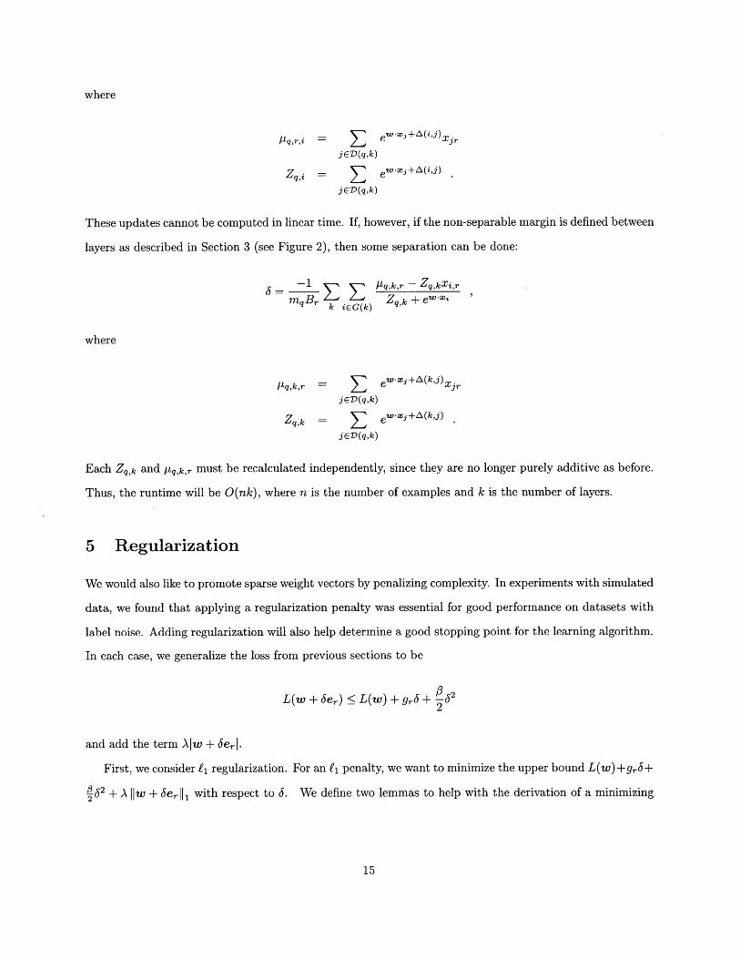
These updates cannot be computed in linear time. If, however, if the non-separable margin is defined between

layers as described in Section 3 (see Figure 2), then some separation can be done:

z = 'r - Z,kxm iG(k) Zq,k + ewx'

where

ILq,k,r = Z ew.xj+s(k,j)XjrjED(q,k)

Zq,k = 1 ew-xj+stk,j)

jED(q,k)

Each Zq,k and Pq,k,r must be recalculated independently, since they are no longer purely additive as before.

Thus, the runtime will be O(nk), where n is the number of examples and k is the number of layers.

5 Regularization

We would also like to promote sparse weight vectors by penalizing complexity. In experiments with simulated

data, we found that applying a regularization penalty was essential for good performance on datasets with

label noise. Adding regularization will also help determine a good stopping point for the learning algorithm.

In each case, we generalize the loss from previous sections to be

L(w + 6er) < L(w) + gr3+ 0622

and add the term AIw + Jerl.

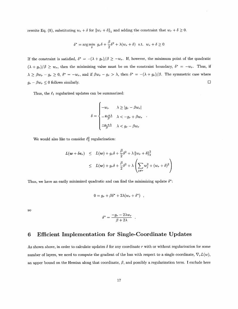
First, we consider f1 regularization. For an f1 penalty, we want to minimize the upper bound L(w) +grJ+

362 + A ||w + 6er||1 with respect to 6. We define two lemmas to help with the derivation of a minimizing

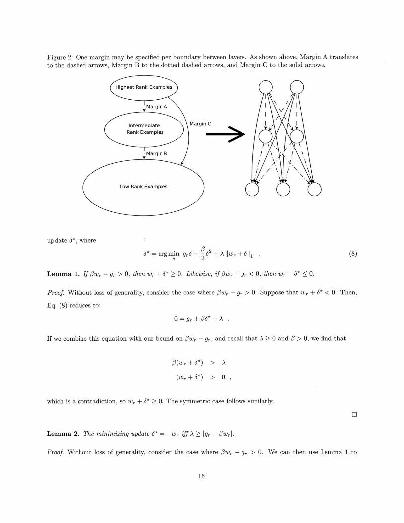
Figure 2: One margin may be specified per boundary between layers. As shown above, Margin A translatesto the dashed arrows, Margin B to the dotted dashed arrows, and Margin C to the solid arrows.

Highest Rank Examples

I \ / \

,Margin A

Intermediate Margin CRank Examples

-Margin B/ \ - / \

/ / \

Low Rank Examples

update 6*, where

arg min g.+ 62+A||w,+6||1 . (8)

Lemma 1. If #wr - gr > 0, then wr + * > 0. Likewise, if #wr - g, < 0, then wr + * < 0.

Proof. Without loss of generality, consider the case where 3w, - gr > 0. Suppose that r + * < 0. Then,

Eq. (8) reduces to:

0=gr+#6*-A

If we combine this equation with our bound on #Wr - gr, and recall that A > 0 and # > 0, we find that

#(Wr + 6*) > A

(Wr +3 *) > 0

which is a contradiction, so wr + 3* > 0. The symmetric case follows similarly.

Lemma 2. The minimizing update * = -wr iff A > |gr - #wr I

Proof. Without loss of generality, consider the case where Ow, - g, > 0. We can then use Lemma 1 to

rewrite Eq. (8), substituting w, + 3 for |w, + Jl and adding the constraint that w, + J 2 0.

* = arg min go + O2 + A(w, + J) s.t. w,+ J > 0

If the constraint is satisfied, * = -(A + gr)/ / -wr. If, however, the minimum point of the quadratic

(A + gr)/# > w,, then the minimizing value must be on the constraint boundary, * = -w,. Thus, if

A > #w, - g, 0, * = -w,, and if #w, - g, > A, then * = -(A + g,)/#. The symmetric case where

gr - #Wr 0 follows similarly. L

Thus, the f1 regularized updates can be summarized:

- Wr

- +A3

A > 9r -3wrl

A < gr +3Wr

A < gr - f3

Wr

We would also like to consider E2 regularization:

L(w + Je,) L(w) + gr + 2 + A ||Wr+ |2

< L(w)+gr3+ j2+ (+A +(w+j)22 A Wj±Q r

Thus, we have an easily minimized quadratic and can find the minimizing update 3*:

0 = g, + OP* + 2A(W, + J*),

so* = -9r - 2AWr

,3+ 2A

6 Efficient Implementation for Single-Coordinate Updates

As shown above, in order to calculate updates 3 for any coordinate r with or without regularization for some

number of layers, we need to compute the gradient of the loss with respect to a single coordinate, VrL(w),

an upper bound on the Hessian along that coordinate, #, and possibly a regularization term. I exclude here

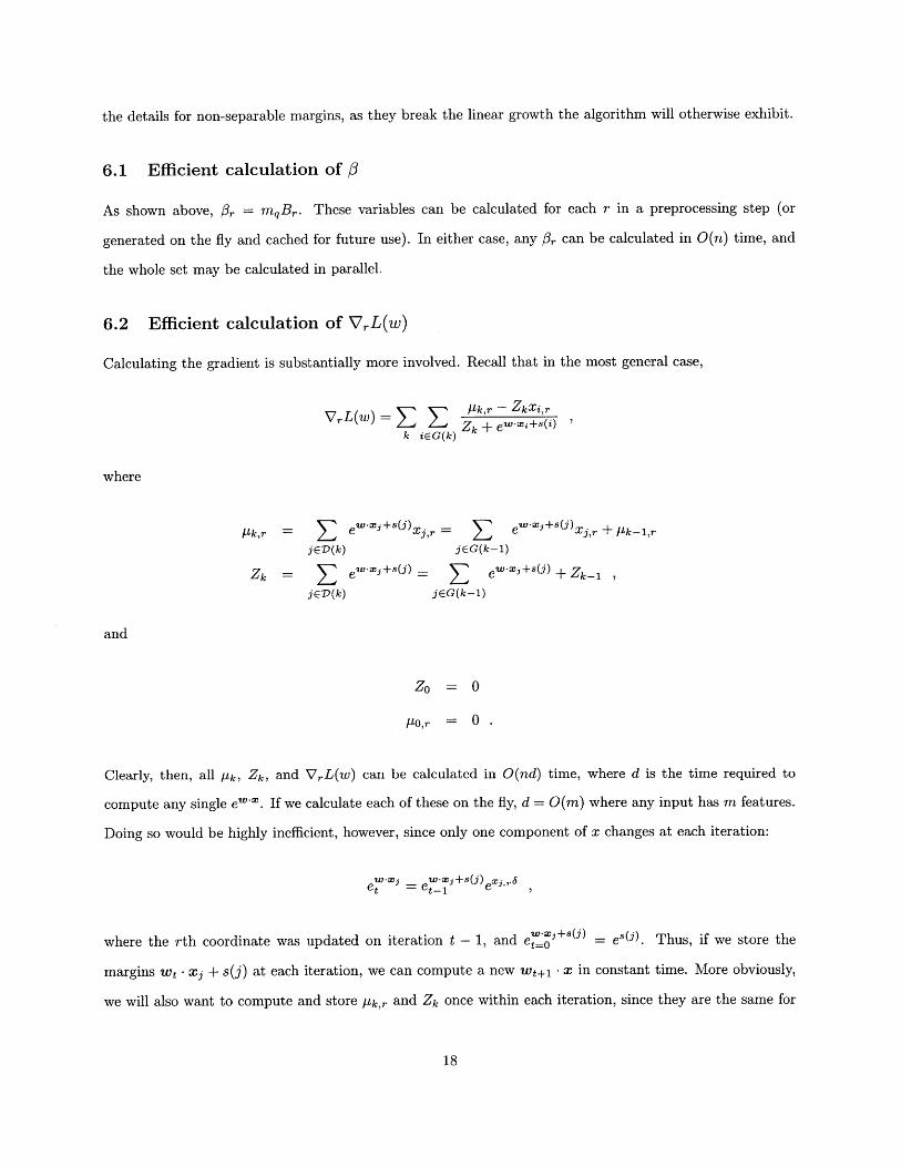
the details for non-separable margins, as they break the linear growth the algorithm will otherwise exhibit.

6.1 Efficient calculation of #

As shown above, #r = mqBr. These variables can be calculated for each r in a preprocessing step (or

generated on the fly and cached for future use). In either case, any f, can be calculated in O(n) time, and

the whole set may be calculated in parallel.

6.2 Efficient calculation of VL(w)

Calculating the gradient is substantially more involved. Recall that in the most general case,

VrL(W) ~ \ / [k,r - ZkXi,rVL(w)= Zk+ ewx'+ ()'

k iGG(k)

where

tk,r = ( ew-+s(j) , ew-oj+s(j)zy,r + /pk-1,r

jGD(k) jEG(k-1)

Zk = E ew-xj+s(j) _ ( ew-x+s(j) + Zk-1

jED(k) jGG(k-1)

and

Zo = 0

PO,r = 0

Clearly, then, all Pk, Zk, and VrL(w) can be calculated in O(nd) time, where d is the time required to

compute any single ew-. If we calculate each of these on the fly, d = 0(m) where any input has m features.

Doing so would be highly inefficient, however, since only one component of x changes at each iteration:

e" ~" = ew-os+s(j)exjgt t-1

where the rth coordinate was updated on iteration t - 1, and e es(j). Thus, if we store the

margins wt -xz + s(j) at each iteration, we can compute a new wt+1 - x in constant time. More obviously,

we will also want to compute and store p-k,, and Zk once within each iteration, since they are the same for

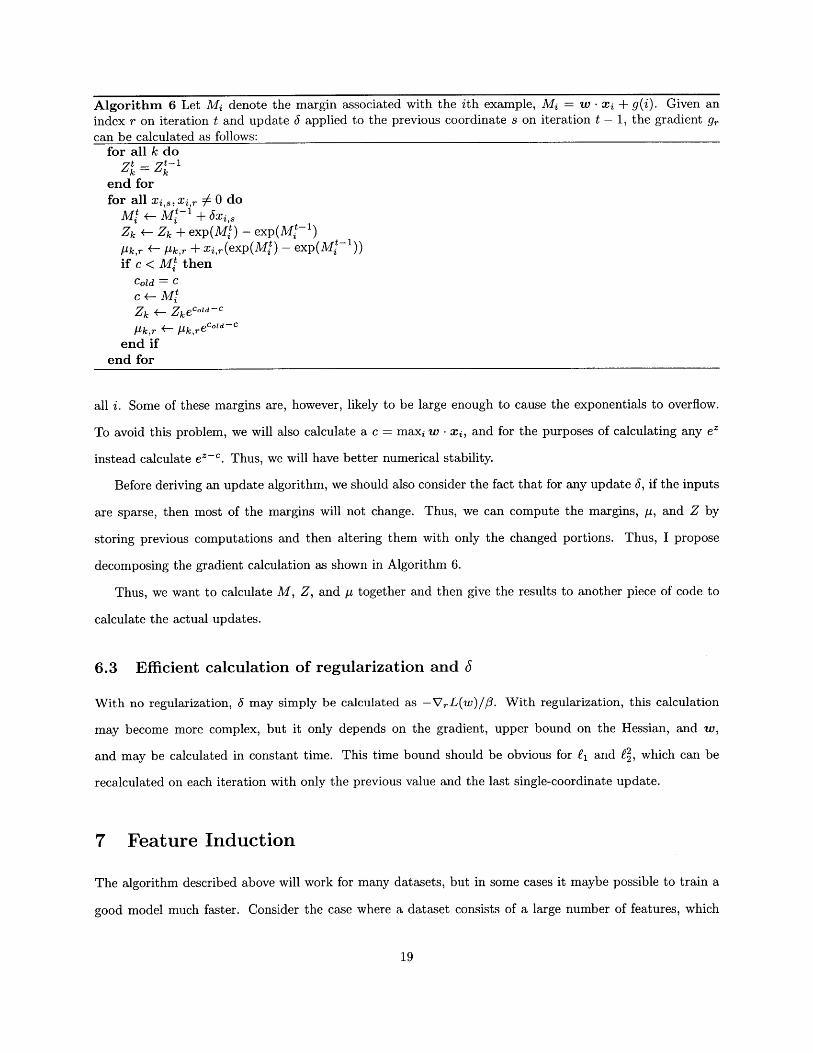
Algorithm 6 Let Mi denote the margin associated with the ith example, M = w - xi + g(i). Given anindex r on iteration t and update J applied to the previous coordinate s on iteration t - 1, the gradient g,can be calculated as follows:

for all k do

Zt = Ztlend forfor all xzi,,, xi,, 7 0 do

Mit +- Mt-1 + oX.~Zk +- Zk + exp(Mt) - exp(Mi 1 )Ik,r +- ph,, + xi,r(exp(Mt) - exp(Mt 1))

if c < Mi thencold = Cc +- Mt

Zk +- Zkecold-c

p-k,r +- Pk,reco'd-c

end ifend for

all i. Some of these margins are, however, likely to be large enough to cause the exponentials to overflow.

To avoid this problem, we will also calculate a c = maxi w - xi, and for the purposes of calculating any ez

instead calculate e2c. Thus, we will have better numerical stability.

Before deriving an update algorithm, we should also consider the fact that for any update 6, if the inputs

are sparse, then most of the margins will not change. Thus, we can compute the margins, y, and Z by

storing previous computations and then altering them with only the changed portions. Thus, I propose

decomposing the gradient calculation as shown in Algorithm 6.

Thus, we want to calculate M, Z, and p together and then give the results to another piece of code to

calculate the actual updates.

6.3 Efficient calculation of regularization and 6

With no regularization, 6 may simply be calculated as -VrL(w)/3. With regularization, this calculation

may become more complex, but it only depends on the gradient, upper bound on the Hessian, and w,

and may be calculated in constant time. This time bound should be obvious for fi and f2, which can be

recalculated on each iteration with only the previous value and the last single-coordinate update.

7 Feature Induction

The algorithm described above will work for many datasets, but in some cases it maybe possible to train a

good model much faster. Consider the case where a dataset consists of a large number of features, which

are mostly sparse for any given instance. If we are using regularization (particularly if we are using f1

regularization with a large regularization weight), our learned weight vector will be sparse. For instance,

when training on a set of images with ten thousand features, we found that a good model was learnable with

only 700 nonzero features. Instead of training on all of these features, then, we could infer which ones will

be useful and focus on training this subset of the features. More concretely, we can bound the change in loss

for an update 6, for feature r:

mqBr 6 2LD(w) - LD(w + 6rer) ;> -rr - m r (9)

Using this bound, we can select the top a features that have the largest minimum decrease in loss. Once we

have trained these until they are close to convergence, we can recalculate the loss bound and add additional

features. See Alg. 7. With sufficient regularization, a lack of good additional features provides a stopping

condition for the algorithm. In experiments, values for a were selected via cross-validation.

Algorithm 7 Feature Induction: The most promising features are chosen, and then trained to convergence.Once no more features remain to train, the algorithm terminates.

{Chosen Features} <-- 0while True do

for each feature r doCalculate gradient g9 and update 6rminlossr < -

6 gr - m-Brr 2

end forSort features by minlossnew-features +- Top a features V {Chosen Features}if new-features == 0 then

breakend if{ Chosen Features} +- {Chosen Features} U new-featuresTrain {Chosen Features} to convergence.

end while

7.1 Stopping Criteria

For most experiments, we simply set a maximum number of iterations as a stopping criterion. For some

smaller datasets, such as the LETOR dataset, the algorithm terminated when the decrease in loss at one

iteration through the features was small compared to the initial change in loss.

Once feature induction was added, though, early termination was easy to achieve. Since only the most

useful features are chosen, and then those are trained to convergence, the model converges much more

quickly. Once there are no new features to select, since all the best features have already converged, training

terminates. In the experiments described in Sec. 8, such convergence with feature induction was common.

8 Results

We have evaluated the domination rank algorithm against four datasets and found it to be competitive with

existing algorithms. We investigate webpage ranking with Microsoft's LETOR dataset, which is of relatively

modest size. We then look at image ranking, specifically at the Corel image datasets and an internal Google

dataset. Finally, we investigate scaling to many features and many instances with Reuters (RCV1) document

ranking.

For each dataset, we endeavored to find a combination of the modifications described above which yield

better performance than other algorithms. In general, the algorithm performs about as well as the best

published results for the various datasets. Some modifications have substantial impact - for instance, feature

selection drastically decreases training time and promotes sparse weight vectors. The datasets are generally

very noisy, and regularization is key to achieving good generalization.

8.1 LETOR Dataset

Microsoft's Learning To Rank (LETOR) [13] consists of nine small datasets with precomputed features. For

each of these datasets, there are associated results from many other algorithms.

8.1.1 Dataset Structure

In LETOR, each dataset consists of a set of queries; for each query, there is a set of documents. These

documents are divided into three layers based on how relevant they are to the query - the most relevant

documents are in layer 2, the mediocre documents in layer 1, and the irrelevant documents in layer 0. The

features are all calibrated against the individual query, so the objective is to find a weighting of these features

that performs well for all queries, thereby ranking the good above the bad on a query by query basis (see Fig.

3). For example, Letor4 contains web pages that correspond to search results, where each page is described

by 46 features that indicate properties like how frequently the search term appears in the document.

Previous work with this dataset has focused on learning a weighting of feature importances on a query-by-

query basis. For instance, the margin between instances is only considered between two documents associated

with the same query.

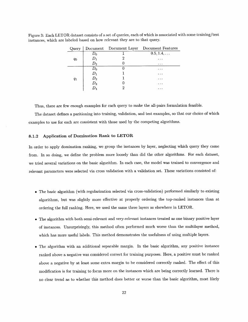
Figure 3: Each LETOR dataset consists of a set of queries, each of which is associated with some training/testinstances, which are labeled based on how relevant they are to that query.

Query Document Document Layer Document FeaturesDo 1 0.5,1.4,....

qo Di 2 ...D2 0 .. .

Do 0 .. .

qi D21---

D3 0 .. .

D4 2 ...

Thus, there are few enough examples for each query to make the all-pairs formulation feasible.

The dataset defines a paritioning into training, validation, and test examples, so that our choice of which

examples to use for each are consistent with those used by the competing algorithms.

8.1.2 Application of Domination Rank to LETOR

In order to apply domination ranking, we group the instances by layer, neglecting which query they came

from. In so doing, we define the problem more loosely than did the other algorithms. For each dataset,

we tried several variations on the basic algorithm. In each case, the model was trained to convergence and

relevant parameters were selected via cross validation with a validation set. These variations consisted of:

" The basic algorithm (with regularization selected via cross-validation) performed similarly to existing

algorithms, but was slightly more effective at properly ordering the top-ranked instances than at

ordering the full ranking. Here, we used the same three layers as elsewhere in LETOR.

" The algorithm with both semi-relevant and very-relevant instances treated as one binary positive layer

of instances. Unsurprisingly, this method often performed much worse than the multilayer method,

which has more useful labels. This method demonstrates the usefulness of using multiple layers.

" The algorithm with an additional separable margin. In the basic algorithm, any positive instance

ranked above a negative was considered correct for training purposes. Here, a positive must be ranked

above a negative by at least some extra margin to be considered correctly ranked. The effect of this

modification is for training to focus more on the instances which are being correctly learned. There is

no clear trend as to whether this method does better or worse than the basic algorithm, most likely

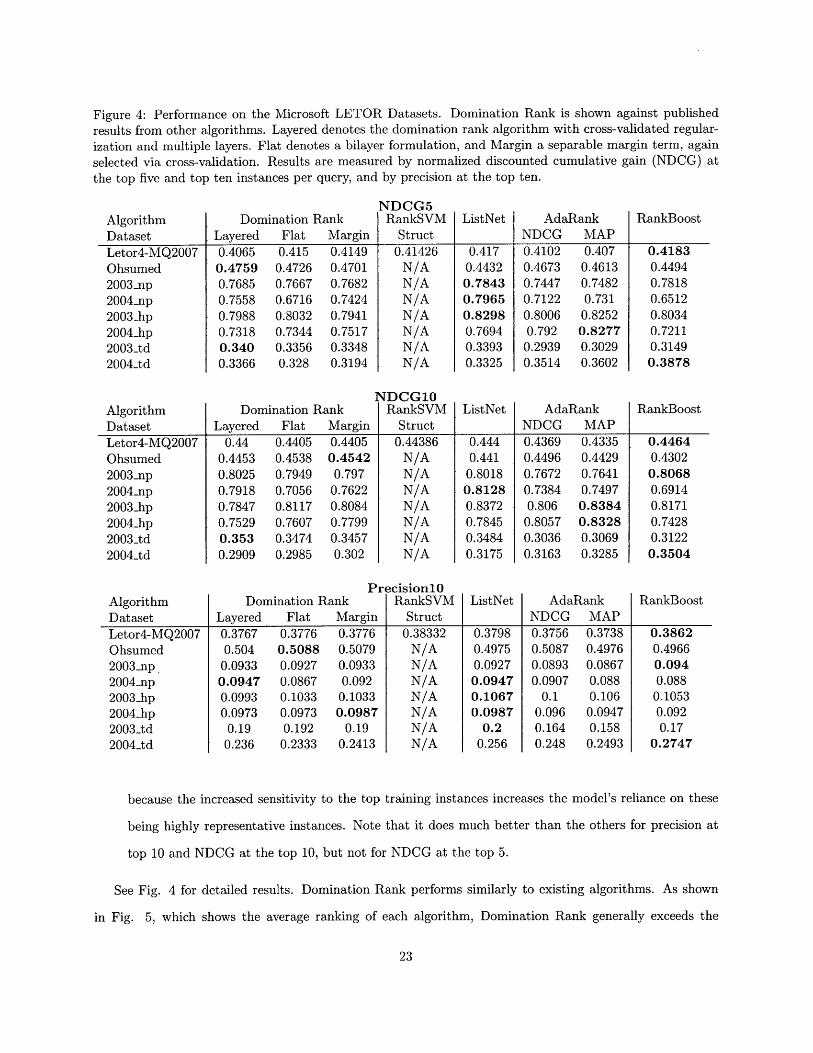
Figure 4: Performance on the Microsoft LETOR Datasets. Domination Rank is shown against publishedresults from other algorithms. Layered denotes the domination rank algorithm with cross-validated regular-ization and multiple layers. Flat denotes a bilayer formulation, and Margin a separable margin term, againselected via cross-validation. Results are measured by normalized discounted cumulative gain (NDCG) atthe top five and top ten instances per query, and by precision at the top ten.

AlgorithmDataset

Domination RankLayered Flat Margin

NDCG5RankSVM

StructListNet Ad

NDCGaRank

MAPRankBoost

Letor4-MQ2007 0.4065 0.415 0.4149 0.41426 0.417 0.4102 0.407 0.4183Ohsumed 0.4759 0.4726 0.4701 N/A 0.4432 0.4673 0.4613 0.44942003_np 0.7685 0.7667 0.7682 N/A 0.7843 0.7447 0.7482 0.78182004_np 0.7558 0.6716 0.7424 N/A 0.7965 0.7122 0.731 0.65122003-hp 0.7988 0.8032 0.7941 N/A 0.8298 0.8006 0.8252 0.80342004 _hp 0.7318 0.7344 0.7517 N/A 0.7694 0.792 0.8277 0.72112003_td 0.340 0.3356 0.3348 N/A 0.3393 0.2939 0.3029 0.31492004_td 0.3366 0.328 0.3194 N/A 0.3325 0.3514 0.3602 0.3878

NDCG1OAlgorithm Domination Rank RankSVM ListNet AdaRank RankBoostDataset Layered Flat Margin Struct NDCG MAPLetor4-MQ2007 0.44 0.4405 0.4405 0.44386 0.444 0.4369 0.4335 0.4464Ohsumed 0.4453 0.4538 0.4542 N/A 0.441 0.4496 0.4429 0.43022003_np 0.8025 0.7949 0.797 N/A 0.8018 0.7672 0.7641 0.80682004_np 0.7918 0.7056 0.7622 N/A 0.8128 0.7384 0.7497 0.69142003_hp 0.7847 0.8117 0.8084 N/A 0.8372 0.806 0.8384 0.81712004_hp 0.7529 0.7607 0.7799 N/A 0.7845 0.8057 0.8328 0.74282003_td 0.353 0.3474 0.3457 N/A 0.3484 0.3036 0.3069 0.31222004_td 0.2909 0.2985 0.302 N/A 0.3175 0.3163 0.3285 0.3504

PrecisionlOAlgorithm Domination Rank RankSVM ListNet AdaRank RankBoostDataset Layered Flat Margin Struct NDCG MAP

Letor4-MQ2007Ohsumed2003_np.2004_np2003_hp2004.hp2003_td2004_td

0.37670.504

0.09330.09470.09930.0973

0.190.236

0.37760.50880.09270.08670.10330.09730.192

0.2333

0.37760.50790.09330.0920.10330.0987

0.190.2413

0.38332N/AN/AN/AN/AN/AN/AN/A

0.37980.49750.09270.09470.10670.0987

0.20.256

0.37560.50870.08930.0907

0.10.0960.1640.248

0.37380.49760.08670.0880.106

0.09470.158

0.2493

0.38620.49660.0940.088

0.10530.0920.17

0.2747

because the increased sensitivity to the top training instances increases the model's reliance on these

being highly representative instances. Note that it does much better than the others for precision at

top 10 and NDCG at the top 10, but not for NDCG at the top 5.

See Fig. 4 for detailed results. Domination Rank performs similarly to existing algorithms. As shown

in Fig. 5, which shows the average ranking of each algorithm, Domination Rank generally exceeds the

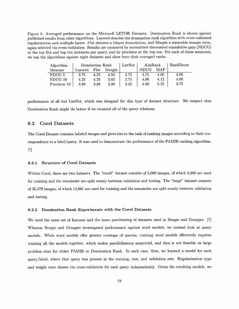
Figure 5: Averaged performance on the Microsoft LETOR Datasets. Domination Rank is shown againstpublished results from other algorithms. Layered denotes the domination rank algorithm with cross-validatedregularization and multiple layers. Flat denotes a bilayer formulation, and Margin a separable margin term,again selected via cross-validation. Results are measured by normalized discounted cumulative gain (NDCG)at the top five and top ten instances per query, and by precision at the top ten. For each of these measures,we ran the algorithms against eight datasets and show here their averaged ranks.

Algorithm Domination Rank ListNet AdaRank RankBoostMeasure Layered Flat Margin NDCG MAPNDCG 5 3.75 4.25 4.50 2.75 4.75 4.00 4.00NDCG 10 4.25 4.25 3.62 2.75 4.88 4.12 4.00Precision 10 3.88 3.88 3.00 2.25 4.88 5.25 3.75

performance of all but ListNet, which was designed for this type of dataset structure. We suspect that

Domination Rank might do better if we retained all of the query relations.

8.2 Corel Datasets

The Corel Dataset contains labeled images and gives rise to the task of ranking images according to their cor-

respondence to a label/query. It was used to demonstrate the performance of the PAMIR ranking algorithm.

[7]

8.2.1 Structure of Corel Datasets

Within Corel, there are two datasets. The "small" dataset consists of 5,000 images, of which 4,000 are used

for training and the remainder are split evenly between validation and testing. The "large" dataset consists

of 35,379 images, of which 14,861 are used for training and the remainder are split evenly between validation

and testing.

8.2.2 Domination Rank Experiments with the Corel Datasets

We used the same set of features and the same partitioning of datasets used in Bengio and Grangier. [7]

Whereas Bengio and Grangier investigated performance against word models, we instead look at query

models. While word models offer greater coverage of queries, training word models effectively requires

training all the models together, which makes parallelization nontrivial, and thus is not feasible on large

problem sizes for either PAMIR or Domination Rank. In each case, then, we learned a model for each

query/label, where that query was present in the training, test, and validation sets. Regularization type

and weight were chosen via cross-validation for each query independently. Given the resulting models, we

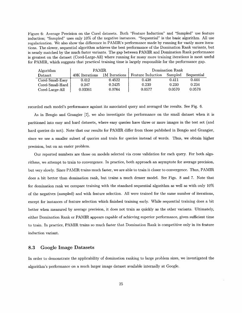
Figure 6: Average Precision on the Corel datasets. Both "Feature Induction" and "Sampled" use featureinduction; "Sampled" uses only 10% of the negative instances. "Sequential" is the basic algorithm. All useregularization. We also show the difference in PAMIR's performance made by running for vastly more itera-tions. The slower, sequential algorithm achieves the best performance of the Domination Rank variants, butis nearly matched by the much faster variants. The gap between PAMIR and Domination Rank performanceis greatest on the dataset (Corel-Large-All) where running for many more training iterations is most usefulfor PAMIR, which suggests that practical training time is largely responsible for the performance gap.

Algorithm PAMIR Domination RankDataset 40K Iterations IM Iterations Feature Induction Sampled SequentialCorel-Small-Easy 0.412 0.4522 0.438 0.411 0.444Corel-Small-Hard 0.247 0.2425 0.230 0.230 0.234Corel-Large-All 0.03361 0.0764 0.0577 0.0570 0.0578

recorded each model's performance against its associated query and averaged the results. See Fig. 6.

As in Bengio and Grangier [7], we also investigate the performance on the small dataset when it is

paritioned into easy and hard datasets, where easy queries have three or more images in the test set (and

hard queries do not). Note that our results for PAMIR differ from those published in Bengio and Grangier,

since we use a smaller subset of queries and train for queries instead of words. Thus, we obtain higher

precision, but on an easier problem.

Our reported numbers are those on models selected via cross validation for each query. For both algo-

rithms, we attempt to train to convergence. In practice, both approach an asymptote for average precision,

but very slowly. Since PAMIR trains much faster, we are able to train it closer to convergence. Thus, PAMIR

does a bit better than domination rank, but trains a much denser model. See Figs. 8 and 7. Note that

for domination rank we compare training with the standard sequential algorithm as well as with only 10%

of the negatives (sampled) and with feature selection. All were trained for the same number of iterations,

except for instances of feature selection which finished training early. While sequential training does a bit

better when measured by average precision, it does not train as quickly as the other variants. Ultimately,

either Domination Rank or PAMIR appears capable of achieving superior performance, given sufficient time

to train. In practice, PAMIR trains so much faster that Domination Rank is competitive only in its feature

induction variant.

8.3 Google Image Datasets

In order to demonstrate the applicability of domination ranking to large problem sizes, we investigated the

algorithm's performance on a much larger image dataset available internally at Google.

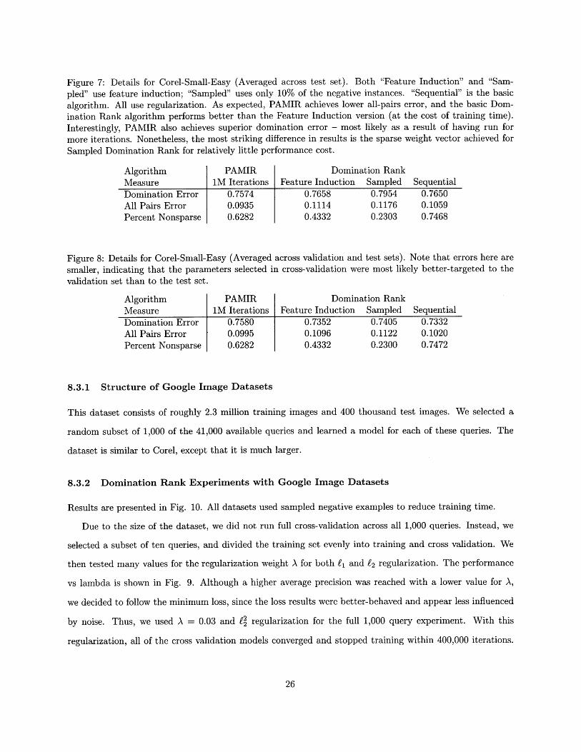
Figure 7: Details for Corel-Small-Easy (Averaged across test set). Both "Feature Induction" and "Sam-pled" use feature induction; "Sampled" uses only 10% of the negative instances. "Sequential" is the basicalgorithm. All use regularization. As expected, PAMIR achieves lower all-pairs error, and the basic Dom-ination Rank algorithm performs better than the Feature Induction version (at the cost of training time).Interestingly, PAMIR also achieves superior domination error - most likely as a result of having run formore iterations. Nonetheless, the most striking difference in results is the sparse weight vector achieved forSampled Domination Rank for relatively little performance cost.

Algorithm PAMIR Domination RankMeasure 1M Iterations Feature Induction Sampled SequentialDomination Error 0.7574 0.7658 0.7954 0.7650All Pairs Error 0.0935 0.1114 0.1176 0.1059Percent Nonsparse 0.6282 0.4332 0.2303 0.7468

Figure 8: Details for Corel-Small-Easy (Averaged across validation and test sets). Note that errors here aresmaller, indicating that the parameters selected in cross-validation were most likely better-targeted to thevalidation set than to the test set.

Algorithm PAMIR Domination RankMeasure 1M Iterations Feature Induction Sampled SequentialDomination Error 0.7580 0.7352 0.7405 0.7332All Pairs Error 0.0995 0.1096 0.1122 0.1020Percent Nonsparse 0.6282 0.4332 0.2300 0.7472

8.3.1 Structure of Google Image Datasets

This dataset consists of roughly 2.3 million training images and 400 thousand test images. We selected a

random subset of 1,000 of the 41,000 available queries and learned a model for each of these queries. The

dataset is similar to Corel, except that it is much larger.

8.3.2 Domination Rank Experiments with Google Image Datasets

Results are presented in Fig. 10. All datasets used sampled negative examples to reduce training time.

Due to the size of the dataset, we did not run full cross-validation across all 1,000 queries. Instead, we

selected a subset of ten queries, and divided the training set evenly into training and cross validation. We

then tested many values for the regularization weight A for both fi and f2 regularization. The performance

vs lambda is shown in Fig. 9. Although a higher average precision was reached with a lower value for A,

we decided to follow the minimum loss, since the loss results were better-behaved and appear less influenced

by noise. Thus, we used A = 0.03 and j2 regularization for the full 1,000 query experiment. With this

regularization, all of the cross validation models converged and stopped training within 400,000 iterations.

We applied the same procedure to find the optimal regularization for PAMIR, and arrived at A = 0.03 for

PAMIR as well.

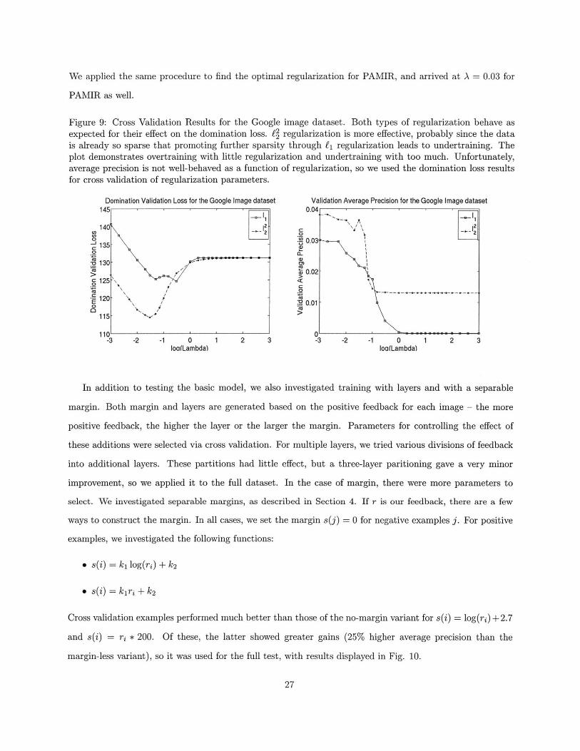
Figure 9: Cross Validation Results for the Google image dataset. Both types of regularization behave asexpected for their effect on the domination loss. f2 regularization is more effective, probably since the datais already so sparse that promoting further sparsity through Li regularization leads to undertraining. Theplot demonstrates overtraining with little regularization and undertraining with too much. Unfortunately,average precision is not well-behaved as a function of regularization, so we used the domination loss resultsfor cross validation of regularization parameters.

Domination Validation Loss for the Google Image dataset Validation Average Precision for the Google Image dataset145 0.04

140d _, 12 2 -

-~0.03135-

130-

> 0.02

O 2-10 7 0.02

115

110 ' 0-3 -2 -1 0 1 2 3 -3 -2 -1 0 1 2 3

loa(Lambda) loa(Lambda)

In addition to testing the basic model, we also investigated training with layers and with a separable

margin. Both margin and layers are generated based on the positive feedback for each image - the more

positive feedback, the higher the layer or the larger the margin. Parameters for controlling the effect of

these additions were selected via cross validation. For multiple layers, we tried various divisions of feedback

into additional layers. These partitions had little effect, but a three-layer paritioning gave a very minor

improvement, so we applied it to the full dataset. In the case of margin, there were more parameters to

select. We investigated separable margins, as described in Section 4. If r is our feedback, there are a few

ways to construct the margin. In all cases, we set the margin s(j) = 0 for negative examples j. For positive

examples, we investigated the following functions:

" s(i) = ki log(ri) + k2

Ss(i) = kiri + k2

Cross validation examples performed much better than those of the no-margin variant for s(i) = log(ri) +2.7

and s(i) = ri * 200. Of these, the latter showed greater gains (25% higher average precision than the

margin-less variant), so it was used for the full test, with results displayed in Fig. 10.

Figure 10: Averaged Results for 1,000 queries on the Google image dataset. Each Domination Rank querywas trained for up to four million iterations, but in practice nearly all stopped before 200,000 iterations.Again, all variations except "Sequential" use feature selection. "Layers" attempts to separate positive imagesinto multiple layers, while "Margin" adds a separable margin based on the positive feedback for each image.Note how close Domination Rank comes to PAMIR's performance with less than 10% as many features.

Algorithm PAMIR Domination RankMeasure 1OOM Iterations 1B Iterations Feature Selection Layers Margin Sequential

Average Precision 0.0552 0.0506 0.0495 0.0495 0.0499 0.0500Precision at Top 10 0.0600 0.0798 0.0731 0.0731 0.0731 0.0731Domination Error 0.9643 0.9625 0.9640 0.9635 0.9643All Pairs Error 0.2344 0.2367 0.2353 0.2367 0.2132Weight Density 0.9663 0.0568 0.0657 0.0676 0.9856

Despite the improvment on the validation set, this margin only had a small effect on the large test. The

margin's effect is fairly sensitive to a small number of images - those with high training relevance - so a

validation set with above-average high-relevance images should see much more improvement than the dataset

as a whole.

It should be noted that the dataset is extremely noisy - many relevant images are mislabeled as negatives

and vice versa. Despite the low test precision, many of the incorrectly high-ranked images are actually highly

relevant to the query.

See Figs. 11 and 12 for a query-by-query plot of Domination Rank and PAMIR performance. Note that

the algorithms perform roughly the same for many of the queries - suggesting those have been learned as well

as is possible given the noise in the dataset - but that for other queries, either algorithm may significantly

outperform the other.

8.3.3 Detailed training analysis

In order to gain insight into the effects of training parameters on the resulting model, we investigate the

performance of a single representative query in the dataset.

First, we investigate performance vs the regularization weight A. As one would expect, increasing A

increases performance on the test set (particularly loss) until it grows too large and causes undertraining.

Note Fig. 13.

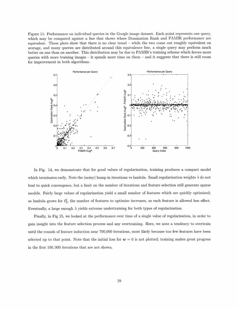
Figure 11: Performance on individual queries in the Google image dataset. Each point represents one query,which may be compared against a line that shows where Domination Rank and PAMIR performance areequivalent. These plots show that there is no clear trend - while the two come out roughly equivalent onaverage, and many queries are distributed around this equivalence line, a single query may perform muchbetter on one than on another. This distribution may be due to PAMIR's training scheme which favors morequeries with more training images - it spends more time on them - and it suggests that there is still roomfor improvement in both algorithms.

Performance per Query Performance per Query0.7- 0.3

0.6- 0.2-

0-

0.5 - .0.1-CL:

.- . .. *. *

> <

*..** -L . -. *,*

0. * -0.3-o * 0

-0.3

0 * ' '-0.40 0.1 0.2 0.3 0.4 0.5 0.6 0.7 0 200 400 600 800 1000

PAMIR AvgP Query Index

In Fig. 14, we demonstrate that for good values of regularization, training produces a compact model

which terminates early. Note the (noisy) hump in iterations vs lambda. Small regularization weights A do not

lead to quick convergence, but a limit on the number of iterations and feature selection still generate sparse

models. Fairly large values of regularization yield a small number of features which are quickly optimized;

as lambda grows for f', the number of features to optimize increases, as each feature is allowed less effect.

Eventually, a large enough A yields extreme undertraining for both types of regularization.

Finally, in Fig 15, we looked at the performance over time of a single value of regularization, in order to

gain insight into the feature selection process and any overtraining. Here, we note a tendency to overtrain

until the rounds of feature induction near 700,000 iterations, most likely because too few features have been

selected up to that point. Note that the initial loss for w = 0 is not plotted; training makes great progress

in the first 100,000 iterations that are not shown.

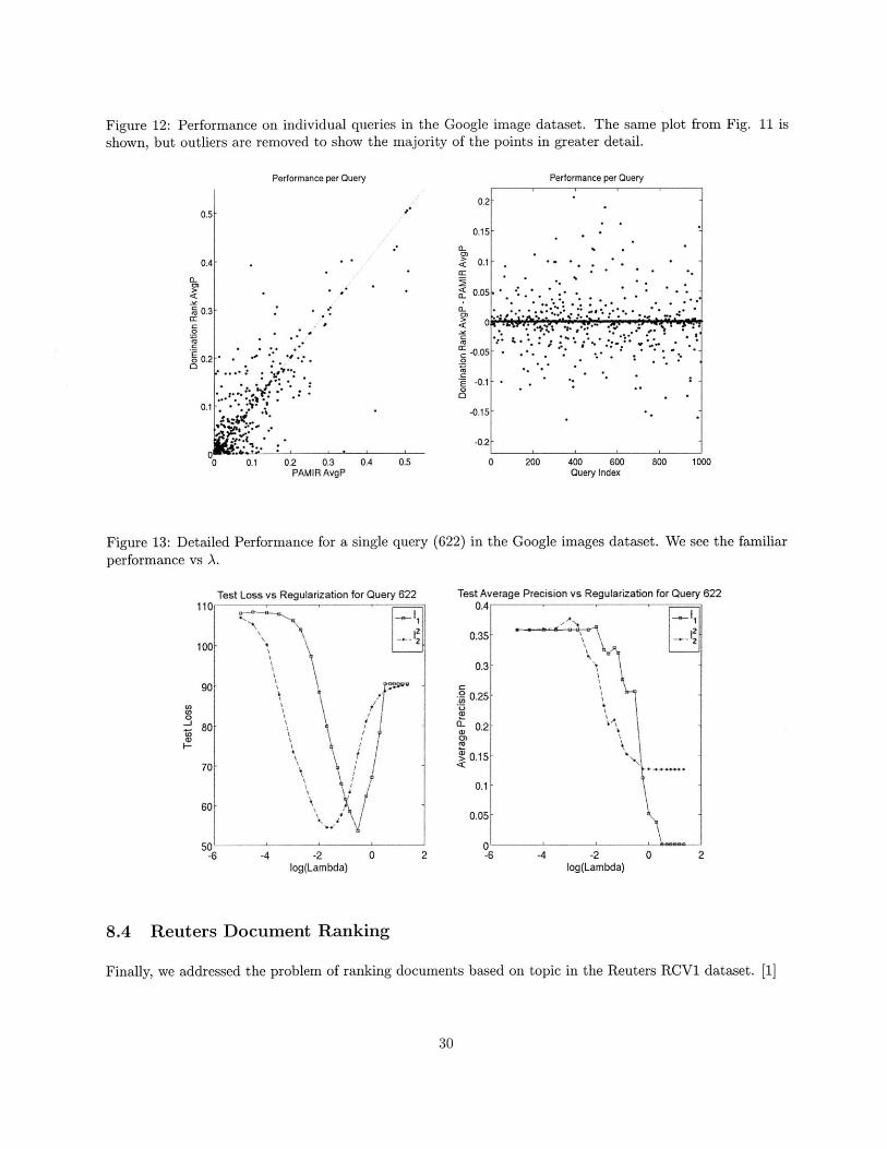
Figure 12: Performance on individual queries in the Google image dataset. The same plot from Fig. 11 isshown, but outliers are removed to show the majority of the points in greater detail.

Performance per Query

7I

.4..

0.1 0.2 0.3 0.4 0.5PAMIR AvgP

Performance per Query

0 200 400 600 800 1000Query Index

Figure 13: Detailed Performance for a single query (622) in the Google images dataset. We see the familiarperformance vs A.

Test Loss vs Regularization for Query 622

- 1-2

-4 -2log(Lambda)

0 2

Test Average Precision vs Regularization for Query 62204A

0.25

0.2

0.15

0.1

0.05

-4 -2log(Lambda)

8.4 Reuters Document Ranking

Finally, we addressed the problem of ranking documents based on topic in the Reuters RCV1 dataset. [1]

0 2

I.I

-

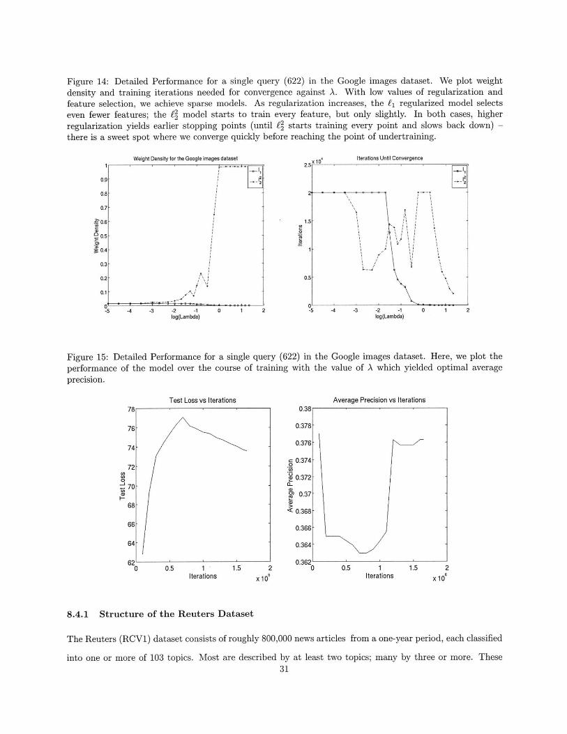
Figure 14: Detailed Performance for a single query (622) in the Google images dataset. We plot weightdensity and training iterations needed for convergence against A. With low values of regularization andfeature selection, we achieve sparse models. As regularization increases, the fi regularized model selectseven fewer features; the f2 model starts to train every feature, but only slightly. In both cases, higherregularization yields earlier stopping points (until f2 starts training every point and slows back down) -there is a sweet spot where we converge quickly before reaching the point of undertraining.

Weight Density for the Google images dataset

0.9- o~g 12

0.8-

0.7

0.6 -

90.5-

0.4-

0.3

0.2-

0.1-

-5 -4 -3 -2 -1log(Lambda)

0 1 2

Figure 15: Detailed Performance for a singleperformance of the model over the course ofprecision.

Iterations Until Convergence

-2 -1log(Lambda)

query (622) in the Google images dataset. Here, we plot thetraining with the value of A which yielded optimal average

Test Loss vs Iterations'Pa''

62'0 0.5 1

Iterations1.5 2

x 106

0.38 -

0.378-

0.376-

0.374-

0.372-

0.37-

0.368-

0.366

0.364-

0.362 -0

Average Precision vs Iterations

0.5 1Iterations

8.4.1 Structure of the Reuters Dataset

The Reuters (RCV1) dataset consists of roughly 800,000 news articles from a one-year period, each classified

into one or more of 103 topics. Most are described by at least two topics; many by three or more. These31

0-70

1.5 2

x 10

topics are hierarchical - for example, there is a general economics category (ECAT) and many subtopics

under it. Associated with each article is the raw text of the article and a set of metadata that includes

title, date published, etc. Articles are fairly evenly split between the four top categories. Thus, the task of

assigning articles in this dataset to topics presents a wide range of ranking tasks - some have much more

data and are much simpler than others. In all cases, though, the articles are hand-labeled, and thus there is

much less label noise than in the prior image experiments.

8.4.2 Application of Domination Rank to the Reuters Dataset

We investigated a couple of different feature sets given this dataset: first, a set of bigrams and associated

appearance counts, and secondly a set of unigrams with features generated as per Crammer and Singer 2003

[5] and Singhal et al 1996 [12]. In each case, we used only the raw text of each article as input and attempted

to find the most relevant articles for each topic.

In order to generate the Singhal features, we applied the following process:

1. Convert upper case characters to lower case

2. Replace non-alphanumeric characters to whitespace

3. Generate a dictionary of all words appearing twice or more. This yielded 225,329 words.

4. Discard the GMIL section, which has too few documents

5. Generate numeric feature values from the words. Each feature xij for word or feature j and document

i is computed using the term frequency tff and the inverse document frequency of a term, idfj,

xij = idfj * tf'

idfj = log(m/rj), where m is the total number of documents and rj is the number of documents

containing word j.tf = (+ log(di)/(1 + log di)

t 1.0 - slope + slope x (mi/A)

where mi is the number of unique words in document i, di is the number of times word j appears in

document i, di is the average frequency of terms in document i, and A is the average number of unique

terms in each document in the corpus. As in [5] and [12}, we set slope = 0.3.

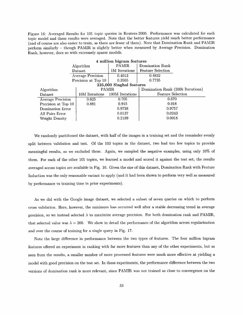
Figure 16: Averaged Results for 101 topic queries in Reuters-2000. Performance was calculated for eachtopic model and these results were averaged. Note that the better features yield much better performance

(and of course are also easier to train, as there are fewer of them). Note that Domination Rank and PAMIRperform similarly - though PAMIR is slightly better when measured by Average Precision. DominationRank, however, does so with extremely sparse models.

4 million bigram featuresAlgorithm PAMIR Domination RankDataset IM Iterations Feature SelectionAverage Precision 0.4013 0.4832Precision at Top 10 0.3505 0.7735

225,000 Singhal featuresAlgorithm PAMIR Domination Rank (200k Iterations)Dataset 10M Iterations 100M Iterations Feature SelectionAverage Precision 0.625 0.705 0.670Precision at Top 10 0.881 0.915 0.918Domination Error 0.9738 0.9757All Pairs Error 0.0137 0.0243Weight Density 0.2189 0.0018

We randomly parititoned the dataset, with half of the images in a training set and the remainder evenly

split between validation and test. Of the 103 topics in the dataset, two had too few topics to provide

meaningful results, so we excluded these. Again, we sampled the negative examples, using only 10% of

them. For each of the other 101 topics, we learned a model and scored it against the test set; the results

averaged across topics are available in Fig. 16. Given the size of this dataset, Domination Rank with Feature

Induction was the only reasonable variant to apply (and it had been shown to perform very well as measured

by performance vs training time in prior experiments).

As we did with the Google image dataset, we selected a subset of seven queries on which to perform

cross validation. Here, however, the minimum loss occurred well after a stable decreasing trend in average

precision, so we instead selected A to maximize average precision. For both domination rank and PAMIR,

that selected value was A = 200. We show in detail the performance of the algorithm across regularization

and over the course of training for a single query in Fig. 17.

Note the large difference in performance between the two types of features. The four million bigram

features offered an experiment in ranking with far more features than any of the other experiments, but as

seen from the results, a smaller number of more processed features were much more effective at yielding a

model with good precision on the test set. In these experiments, the performance difference between the two

versions of domination rank is more relevant, since PAMIR was not trained as close to convergence on the

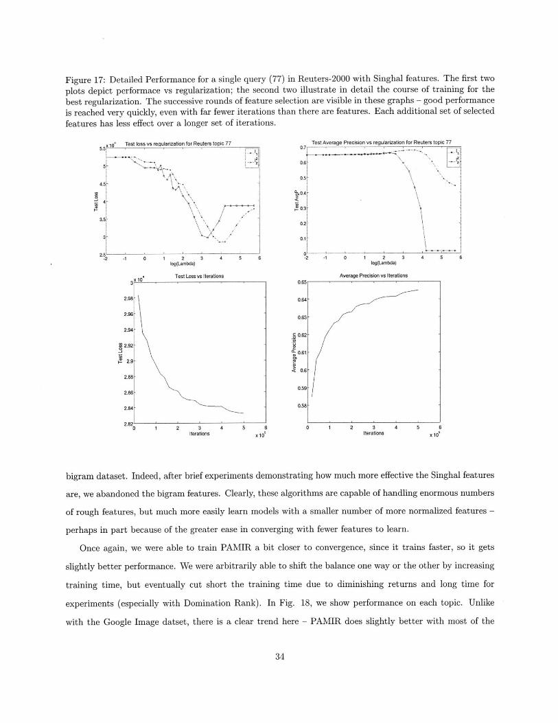
Figure 17: Detailed Performance for a single query (77) in Reuters-2000 with Singhal features. The first two

plots depict performace vs regularization; the second two illustrate in detail the course of training for the

best regularization. The successive rounds of feature selection are visible in these graphs - good performanceis reached very quickly, even with far fewer iterations than there are features. Each additional set of selectedfeatures has less effect over a longer set of iterations.

x104 Test loss vs regularization for Reuters topic 775.5i

4.5

40

3.5:_

3

2 1 0 1 2 3 4 5 6

slO

log(Lamtxta)

Test Loss vs Iterations

82'0 1 2 3

Iterations4 5 6

X 10s

Test Average Precision vs regularization for Reuters topic 770.7

0.6--

0.5 -

0.3

0.2

0.11

0 --2 -1 0 1 2 3 4 5 6

log(Lambda)

Average Precision vs Iterations0.65

0.64-

0.63-

A 0.62 -

00.61-

< 0.6-

0.59-

0.58-

4 5 6X 10

0 1 2 3Iterations

bigram dataset. Indeed, after brief experiments demonstrating how much more effective the Singhal features

are, we abandoned the bigram features. Clearly, these algorithms are capable of handling enormous numbers

of rough features, but much more easily learn models with a smaller number of more normalized features -

perhaps in part because of the greater ease in converging with fewer features to learn.

Once again, we were able to train PAMIR a bit closer to convergence, since it trains faster, so it gets

slightly better performance. We were arbitrarily able to shift the balance one way or the other by increasing

training time, but eventually cut short the training time due to diminishing returns and long time for

experiments (especially with Domination Rank). In Fig. 18, we show performance on each topic. Unlike

with the Google Image datset, there is a clear trend here - PAMIR does slightly better with most of the

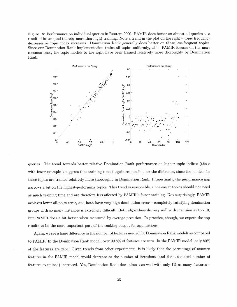
Figure 18: Performance on individual queries in Reuters-2000. PAMIR does better on almost all queries as aresult of faster (and thereby more thorough) training. Note a trend in the plot on the right - topic frequencydecreases as topic index increases. Domination Rank generally does better on these less-frequent topics.Since our Domination Rank implementation trains all topics uniformly, while PAMIR focuses on the morecommon ones, the topic models to the right have been trained relatively more thoroughly by DominationRank.

Performance per Query Performance per Query1 0.3

0.9- . .25-

0.8--- 0.2-

0.7 .

a. * . '0.15-

<0.6 - ** a.* a. 0.1

-.5 -> .

0.05-0.4 0 0

0 .. .. .... ...

0.3- **%*

0

0.2 - 0 -0.05 - - --

0.1 -0.1

. '-0.150 0.2 0.4 0.6 0.8 1 0 20 40 60 80 100 120

PAMIR AvgP Query Index

queries. The trend towards better relative Domination Rank performance on higher topic indices (those

with fewer examples) suggests that training time is again responsible for the difference, since the models for

these topics are trained relatively more thoroughly in Domination Rank. Interestingly, the performance gap

narrows a bit on the highest-performing topics. This trend is reasonable, since easier topics should not need

as much training time and are therefore less affected by PAMIR's faster training. Not surprisingly, PAMIR

achieves lower all-pairs error, and both have very high domination error - completely satisfying domination

groups with so many instances is extremely difficult. Both algorithms do very well with precision at top 10,

but PAMIR does a bit better when measured by average precision. In practice, though, we expect the top

results to be the more important part of the ranking output for applications.

Again, we see a large difference in the number of features needed for Domination Rank models as compared

to PAMIR. In the Domination Rank model, over 99.8% of features are zero. In the PAMIR model, only 80%

of the features are zero. Given trends from other experiments, it is likely that the percentage of nonzero

features in the PAMIR model would decrease as the number of iterations (and the associated number of

features examined) increased. Yet, Domination Rank does almost as well with only 1% as many features -

it is extremely effective at identifying the most relevant features. While it might be possible to formulate

a version of PAMIR that also achieves such sparsity (the formulation shown here uses 6l regularization

which does not promote sparsity), Domination Rank has an intrinsic advantage at learning sparse models,

since it considers the effect of all instances of a given feature before deciding whether to use that feature,

and skips the less useful ones. A pair-by-pair examination of features like what PAMIR does could easily

exclude an extremely useful feature apparent in all pairs, but only marginally useful in any single pair.

Thus, Domination Rank's consideration of every appearance of a feature, while responsible for much of the

longer training time, is extremely useful whenever a sparse model is desired. For examples of the progress

of training with feature selection, see Fig. 17. Note that the top features have a very quick, very substantial

impact on training.

9 Conclusions

We derive a coordinate descent algorithm for finding a ranking based on the Domination Error which Dekel

et al. [10] showed to be a promising candidate for a ranking algorithm. We find a convex relaxation of that

error and associated updates which scale linearly with the number of training instances, even for many layers

of training data labels.

Given this basic algorithm, we derive and try experimentally a number of variations. Multilayer training

allows the algorithm to handle datasets where we have more detailed feedback as to which instances are

most relevant. A separable margin gives us a similar ability to increase the influence of certain (high margin)

instances. f1 and f2 regularization, one of which is used in every experiment, vastly increases the algorithm's

robustness against noise. Feature induction speeds up training by reducing time spent on mediocre features

and yields very sparse models with performance almost as good as that of dense models. We show that most

of each update may be stored from previous rounds, again increasing the speed of training, and demonstrate

the stability of the coordinate descent updates.

We apply the algorithm to a number of datasets. On the LETOR dataset, we find that Domination Rank

performs similarly to existing algorithms at ranking a small dataset of web documents with few features.

Using multiple layer labels, when such labels are available, slightly increases performance. With the Corel and

Google Images datasets, Domination Rank performs similarly to the highly effective PAMIR algorithm, but

with longer training times and ultimately more compact models. Feature induction and sampling negative

instances greatly decrease training time, while greatly increasing model sparsity and slightly decreasing

performance. We apply these lessons to experiments with the Reuters RCV1 dataset, which provides a

trial on a large dataset with far more features than prior datasets. PAMIR and Domination Rank perform

well, especially with Singhal's features, and demonstrate effective and extremely sparse models learned by

Domination Rank.

References

[1] Reuters corpus vol 1. 2000. Available at http://about.reuters.com/researchandstandards/corpus/.

[2} S. Boyd and L. Vandenberghe. Convex Optimization. Cambridge University Press, 2004.

[3] Michael Collins. Ranking algorithms for named-entity extraction: Boosting and the voted perceptron.

In Association for Computational Linguistics (A CL), pages 489-496, 2002.

[4] Michael Collins and Terry Koo. Discriminative reranking for natural language parsing. In International

Conference on Machine Learning (ICML), 2000.

[5] Koby Crammer and Yoram Singer. A family of additive online algorithms for category ranking. J.

Mach. Learn. Res., 3:1025-1058, 2003.

[6] A. Elisseeff and J. Weston. A kernel method for multi-labelled classification. NIPS, 14, 2001.

[7] David Grangier and Samy Bengio. A discriminative kernel-based model to rank images from text queries.

IEEE Transactions on Pattern Analysis and Machine Intelligence, 30(8):1371-1384, August 2008.

[8] H. Li J. Xu. Adarank: A boosting algorithm for information retrieval. SIGIR, 2007.

[9] G. Lebanon and J. Lafferty. Cranking: Combining rankings using conditional probability models on

permutations. Proceedings of the Nineteenth International Conference on Machine Learning, 2002.

[10] C. Manning 0. Dekel and Y. Singer. Log-linear models for label ranking. In Neural Information

Processing Systems (NIPS), 2003.

[11] Robert Schapire and Yoram Singer. Improved boosting algorithms using confidence-rated predictions.

1999.

[12] Amit Singhal, Chris Buckley, and Mandar Mitra. Pivoted document length normalization. In SIGIR

'96: Proceedings of the 19th annual international ACM SIGIR conference on Research and development

in information retrieval, pages 21-29, New York, NY, USA, 1996. ACM.

[131 T. Qin W. Xiong T. Liu, J. Xu and H. Li. Letor: Benchmark dataset for research on learning to rank

for information retreival. SIGIR, 2007.

[141 R. Schapire Y. Singer Y. Freund, R. Iyer. An efficient boosting algorithm for combining preferences.

2003.

[15] et al Z. Cao. Learning to rank: From pairwise approach to listwise approach. ICML, 227.