Master Thesis Simulation of communication within robotic fleet in agricultural environment under the supervision of Dipl.Ing. Dr. techn. Slobodanka Tomic Univ.Prof. Dr.Ing. Christoph Mecklenbräuker Institute of Telecommunications, E389 Department of Electrical Engineering Vienna University of Technology By Mariona Roca Ros Wien, May 23, 2012

Welcome message from author
This document is posted to help you gain knowledge. Please leave a comment to let me know what you think about it! Share it to your friends and learn new things together.
Transcript
Master Thesis
Simulation of communication within robotic fleet in agricultural environment
under the supervision of
Dipl.-‐Ing. Dr. techn. Slobodanka Tomic Univ.Prof. Dr.-‐Ing. Christoph Mecklenbräuker
Institute of Telecommunications, E389 Department of Electrical Engineering Vienna University of Technology
By
Mariona Roca Ros
Wien, May 23, 2012
Simulation of communication within robotic fleet in agricultural environment Mariona Roca Ros
2
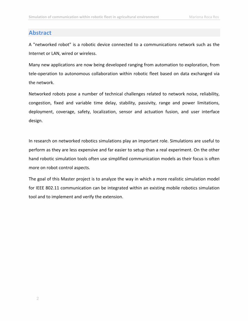
Abstract
A "networked robot" is a robotic device connected to a communications network such as the
Internet or LAN, wired or wireless.
Many new applications are now being developed ranging from automation to exploration, from
tele-‐operation to autonomous collaboration within robotic fleet based on data exchanged via
the network.
Networked robots pose a number of technical challenges related to network noise, reliability,
congestion, fixed and variable time delay, stability, passivity, range and power limitations,
deployment, coverage, safety, localization, sensor and actuation fusion, and user interface
design.
In research on networked robotics simulations play an important role. Simulations are useful to
perform as they are less expensive and far easier to setup than a real experiment. On the other
hand robotic simulation tools often use simplified communication models as their focus is often
more on robot control aspects.
The goal of this Master project is to analyze the way in which a more realistic simulation model
for IEEE 802.11 communication can be integrated within an existing mobile robotics simulation
tool and to implement and verify the extension.
Simulation of communication within robotic fleet in agricultural environment Mariona Roca Ros
3
Acknowledgments
I would first like to thank Slobodanka Tomic for giving me the oportunity of doing my master
thesis with her in FTW and leting me take part of the RHEA project, it has been a great
experience. Also for her pacience, time and understanding.
I also want to give special thanks to Christoph Mecklenbräuker for the help and the advice.
My gratitude also goes to the FTW team. It is great to work in such a nice environment. Special
thanks to Thomas, for the support in the last moments of stress and for being at the other side
of Skype at any hour. To Mirko and Piero for the support, for the nice coffee times and for some
crazy party I will always remember. And to the rest of the people with whom I shared some
special moments there.
I would also like to thank all the people who made my Erasmus special. Special thanks to some
of them, like Tatiana, for being such a good friend and confident. Dominik, you made me feel at
home. Sergi, Laura and Alex, for the great times spent together.
After many years at the university I feel so lucky of having shared such great times with very
nice people. To all of them, thanks for making these hard times a bit funnier and greater. And
specially for making me not feel alone.
But my erasmus, my stage at FTW and my student life in general would not have been the same
if it wasn’t for Jordi Vallcorba. I still cannot understand why we always passed and failed the
same lectures, why we coincided in choosing Vienna as a destination, why we finally did the
master thesis at the same company and at the end even at the same room! I feel so lucky of
having had such a tween soul during all these years. Thanks for everything, Jordi!
I’d also like to give special thanks to my family, for the inconditional support and for filling my
head with the values I’m proud of.
And finally, I must thank a person who, even staying long periods far from me has always been
by my side and has always supported and trusted me. It is a pleasure to keep sharing my neuron
with you. T’estimo, Jordi.
Simulation of communication within robotic fleet in agricultural environment Mariona Roca Ros
4
Contents
Abstract ......................................................................................................................................................... 2
Acknowledgments ......................................................................................................................................... 3
Contents ........................................................................................................................................................ 4
List of figures ................................................................................................................................................. 6
List of tables .................................................................................................................................................. 7
1. Introduction .......................................................................................................................................... 8
1.1 Background ................................................................................................................................... 8
• Multiple mobile robot systems ................................................................................................... 10
• Networked robots ....................................................................................................................... 12
• EU RHEA project .......................................................................................................................... 13
1.2 Problem Statements .................................................................................................................... 19
1.3 Outline of Thesis ......................................................................................................................... 19
2. Communication in Robotic Fleets in Agriculture ................................................................................. 21
2.1 Application of Robotic Fleets ...................................................................................................... 21
2.2 Fleet Communication Requirements and Performance Criteria ................................................. 21
2.3 OSI Model .................................................................................................................................... 23
2.4 Communication Technology -‐ WLAN .......................................................................................... 24
• IEEE 802.11 .................................................................................................................................. 25
• Physical layer frame structure ..................................................................................................... 26
• Frame reception process ............................................................................................................. 27
• Benefits ....................................................................................................................................... 29
• Limitations ................................................................................................................................... 29
3. Simulation of Robotic Systems and Mobile Networks ........................................................................ 30
3.1 Introduction ................................................................................................................................ 30
3.2 Existing Platforms ........................................................................................................................ 30
3.3 Webots Simulation of robotic fleets ........................................................................................... 31
3.4 NS-‐2 Simulation of mobile networks ........................................................................................... 32
3.4.1 General Information ............................................................................................................ 32
3.4.2 Simulation Models .............................................................................................................. 33
4. Realization of the Communication Stack in Webots ........................................................................... 36
Simulation of communication within robotic fleet in agricultural environment Mariona Roca Ros
5
4.1 Architecture ................................................................................................................................ 36
• Application layer ......................................................................................................................... 37
• MAC layer .................................................................................................................................... 37
• Physical layer ............................................................................................................................... 39
• Prereceive layer ........................................................................................................................... 40
4.2 Implementation ........................................................................................................................... 40
• How time is managed .................................................................................................................. 40
• Adaptation of the emitter node in Webots ................................................................................. 44
• Propagation models .................................................................................................................... 45
• Metrics ........................................................................................................................................ 49
• Rebroadcast mechanism ............................................................................................................. 53
4.3 Suggested Improvements ........................................................................................................... 53
5. Evaluation ........................................................................................................................................... 54
5.1 Performance Criteria ................................................................................................................... 54
5.2 Simulation Scenarios ................................................................................................................... 54
• Propagation models .................................................................................................................... 54
• Rebroadcast mechanism ............................................................................................................. 58
• Robot movement ........................................................................................................................ 61
• Priority mechanisms .................................................................................................................... 64
5.3 Processing of simulation results .................................................................................................. 67
5.4 Discussion of results .................................................................................................................... 67
5.5 Possible extensions ..................................................................................................................... 69
6. Conclusion ........................................................................................................................................... 71
6.1 Contribution ................................................................................................................................ 71
6.2 Outlook ........................................................................................................................................ 72
7. References .......................................................................................................................................... 75
Appendixes .................................................................................................................................................. 77
Appendix A: Definition of the most important classes ......................................................................... 77
Appendix B: Modification of the node emitter.wrl ............................................................................... 83
Appendix C: Results of the simulations ................................................................................................. 85
Appendix E: User manual ....................................................................................................................... 89
Simulation of communication within robotic fleet in agricultural environment Mariona Roca Ros
6
List of figures
Figure 1 The logical position and relationships of the HLDMS with the rest of the subsystems .. 14
Figure 2 802.11 Layer architecture ............................................................................................... 26
Figure 3 IEEE 802.11 frame format ............................................................................................... 27
Figure 4 IEEE 802.11a wireless standard definition of the MAC and Physical layer ..................... 33
Figure 5 Carrier sense multiple access with collision avoidance (CSMA/CA) mechanism ............ 34
Figure 6 Architecture of the implementation of the communication stack in Webots ................ 36
Figure 7 Implementation of the MAC layer in NS2 ....................................................................... 39
Figure 8 Implementation of the Physical layer in NS2 .................................................................. 40
Figure 9 List scheduler .................................................................................................................. 41
Figure 10 Desired scheduler situations. RTS and ACK packets are received before the respective timers expire. ................................................................................................................................ 42
Figure 11 Scheduler before scaling. RTS and ACK packets are received once the respective timers expire. ........................................................................................................................................... 42
Figure 12 Free Space Loss propagation model ............................................................................. 46
Figure 13 Two Ray Interference model ......................................................................................... 46
Figure 14 Plane Earth propagation model .................................................................................... 47
Figure 15 Weissberger's Modified Exponential decay model ....................................................... 47
Figure 16 The effect of the implemented propagation models in the standards IEEE 802.11a and IEEE 802.11g ................................................................................................................................. 49
Figure 17 Examples of value-‐delay functions ................................................................................ 50
Figure 18 Definition of the different packet delays ...................................................................... 51
Figure 19 Examples of value-‐delay functions with a threshold at 0.5 .......................................... 52
Figure 20 When adding metrics mechanism, the queue between the Application and the MAC layer must be chenged for more than one priority queue. .......................................................... 52
Figure 21 Geometrical parameters of a realistic RHEA scenario with olive tree crop .................. 55
Figure 22 different situations depending on the position of the Base Station ............................. 56
Figure 23 first disposition of the robots in the field ..................................................................... 58
Figure 24 second disposition of the robots in the field ................................................................ 59
Simulation of communication within robotic fleet in agricultural environment Mariona Roca Ros
7
Figure 25 third disposition of the robots in the field .................................................................... 59
Figure 26 Maximum possible range in a completely aligned disposition of the robots using Weisberger’s propagation model ................................................................................................. 60
Figure 27 Equally division of the space, so each region corresponds to the action zone of each robot, in a realistic RHEA scenario ................................................................................................ 61
Figure 28 initial distribution of the robots in the field, in a scenario where robots move through the rows in an olive tree crop ....................................................................................................... 61
Figure 29 simulated flow of data between the base station (BS) and the robots 2, 3 and 4 ........ 62
Figure 30 Simulated flows of data between the robots. The colored one uses priorities, while in the non-‐colored one all the packets have the same importance ................................................. 65
Figure 31 Different value functions depending on the delay of the packet. At the left side, a soft deadline function. At the right side, a hard deadline function. Both have a threshold that defines two regions with different priorities. ............................................................................................ 66
Figure 32 Trace structure. ............................................................................................................. 67
List of tables
Table 1 dialogue between the Mission Manager and the High-‐Level Decision Making System of each Ground Mobile Unit ............................................................................................................. 17
Table 2 dialogue between the Mission Manager and the High-‐Level Decision Making System of each Ground Mobile Unit ............................................................................................................. 17
Table 3 Specifications of Transmission power and frequency of the standards 802.11a and 802.11g ......................................................................................................................................... 18
Table 4 parameters of the RHEA scenario .................................................................................... 56
Table 5 communication parameters ............................................................................................. 56
Table 6 Results of the first simulation. ......................................................................................... 86
Table 7 Results of the second simulation ..................................................................................... 86
Table 8 Results of the third simulation ......................................................................................... 87
Table 9 Results of the fifth simulation .......................................................................................... 88
Simulation of communication within robotic fleet in agricultural environment Mariona Roca Ros
8
1. Introduction
1.1 Background
Technological developments have recently made a great impact over agriculture and forestry.
Mobile computing can log the yield during harvesting, and global positioning by satellite (GPS)
can help in mapping and guidance operations. Computing leads to the ability of analyzing
images from cameras, as well as vision sensing has pervaded sorting operations, vision guidance
and recognition of animals. This progress in computer power makes agriculture and forestry be
safer and more efficient.
In forestry, for example, CAN (Controller Area Network) based distributed control and
information system, with GPS localization using mobile communication networks to transfer
data relating to harvesting, are being used nowadays. However, GPS does not work well enough
in a forest environment, and simultaneous localization and mapping (SLAM) algorithms are
needed, since the main problem for autonomous harvesters is to detect and parameterize the
valuable trees among other plants and nonvaluable trees.
In the other side, some other new technological solutions such as walking locomotion
mechanism have been developed. Combined with semiautomatic control of forest harvesters
helps increasing efficiency and safety in the system, while human operators can remotely
control the machines. This machines should be intelligent enough that less efficient wireless
communication is sufficient for their operation.
In conclusion, reliable perception and measurement of essential objects and state parameters
in real time is the bottleneck to developing more enhanced autonomous or teleoperated
functions and operations in forestry machines.
In broad acre applications there have also been a great technological advance. With the
convergence of computing and entertainment, cameras can now be directly interfaced through
universal serial bus (USB) ports. Processing power and software are abundant. Differential
carrier-‐based techniques allow low-‐cost GPS receivers to offer centimetre displacement tracking
Simulation of communication within robotic fleet in agricultural environment Mariona Roca Ros
9
and the new generation of systems combine vision, GPS, and inertial sensors. All this help
providing automatic guidance in broad acre applications.
New achievements have also been made in horticulture, where harvesting can require selection
and sensing. Therefore intelligent picking has presented a challenge to many robotics
researchers, since GPS is unreliable under the tree canopy.
Some systems consist in combining odometry with tree-‐trunk location using both sideways-‐
looking visual streaming and radio frequency identification (RFID) tagging, when picking fruits or
kernel from tree plants.
Colour or skin texture sorting are some factors used to determine the quality of the fruits, even
the criteria always depends on the type of fruit to be picked. For example, the grade of ripening
is different in the case of a tomato or a macadamia nut crop. Today, the vision grading system
could well be carried on the harvesting vehicle. There is a growing appreciation of the benefits
of single-‐handling, with grading and packing being performed in the field as part of the picking
operation.
In working with livestock, developments in several aspects such as milking or sheep shearing are
still being done.
During the milking process, all the operations to be done required the supervision of a human
(identifying the cow or assessing the milk, for example), even the presence of milking robots,
some years ago. Nevertheless, nowadays it is the cow’s responsibility to determine the time of
milking. The visit to the milking station is rewarded with grain feeding, but still training is
required to establish a routine.
In sheep shearing some improvements have also been achieved, like an hydraulic robot single-‐
arm or a two-‐armed system. However, even it seemed a great improvement in this field, the
systems ran out of funding because reaching a reasonable speed increased too much the cost
efficiency.
An aspect that makes shearing arduous is the need to manhandle the sheep, while the robot
demanded the sheep to be presented in a structured manner. Therefore, an other system has
been developed, in which the legs of the sheep are cuffed, presenting the sheep at various
Simulation of communication within robotic fleet in agricultural environment Mariona Roca Ros
10
attitudes for the convenience of manual shearers who can now perform their task standing up
rather than crouching, each specializing in a different part of the fleece.
Other new developments have been recently achieved in slaughtering livestock, or in its
inspection.
To address tasks in agriculture, a rise in the use of unmanned aerial vehicles (UAVs) have been
produced. UAV collaborative, which has a cooperative research agreement with the NASA, uses
long duration flight time UAVs to perform unmanned flight operations.
While full-‐sized tractors may never be fully autonomous, there is scope for smaller, cooperative
vehicles to perform set tasks. Many researchers are currently investigating various platforms.
The idea behind smaller units will be that they can work cooperatively and constantly, thus
providing the same amount of horsepower with much reduced risk.
All these developments in the technologies applied to agriculture and forestry make us
introduce some concepts like multiple mobile robot systems and networked robots, which will
help introducing the problems this thesis aims to face.
• Multiple mobile robot systems
The advantages of multirobot systems over single-‐robot systems are the fact that they can carry
a higher task complexity, the distribution of the task between the robots of the system, the ease
to build several resource-‐bounded robots than a single powerful robot, and the faster problem
solving by using parallelism or the robustness through redundancy.
Historically, approaches to multiple mobile robot systems can be distinguished within two broad
categories: collective swarm systems and intentionally cooperative systems. The first is designed
for a large number of homogeneous mobile robots that execute their own tasks with only
minimal need for knowledge about other robot team members. In the latest, the robots have
knowledge of the other robots in the environment and act together based on the state, actions
or capabilities of their teammates in order to accomplish the same goal. This intentionally
Simulation of communication within robotic fleet in agricultural environment Mariona Roca Ros
11
cooperative systems can be divided into Strongly cooperative systems or Weakly cooperative
systems, depending on the dependence on the other robots in taking decisions.
Some team architectures are possible within the system. The most common are centralized,
hierarchical, decentralized, and hybrid. Centralized and hierarchical architectures present
several drawbacks while the actions of some robots depend on a single node. Decentralized and
hybrid are the most used, as no dependencies between robots are defined. Nevertheless, the
more decentralized the system is, the more it requires the high-‐level goal to be incorporated
into the local control of each robot in order to achieve global coherency. Therefore, hybrid
seems to be the best architecture as it combines local control with higher-‐level control
approaches to achieve both robustness and the ability to influence the entire team’s actions
through global goals, plans, or control.
A fundamental assumption in multirobot system research is that global coherent and efficient
goals can be reached through the interaction of robots lacking complete global information. It
requires the robots to obtain information about their teammates. Some techniques can be used
to obtain this information: stigmergy (implicit communication through the world), in which
robots sense the effects of teammate’s actions through their effects on the world, passive
action recognition, in which robots use sensors to directly observe the actions of their
teammates; or explicit communication, in which robots directly and intentionally communicate
relevant information through some active means, such as radio.
Stigmergy and passive action recognition are appealing because of the lack of dependence upon
explicit communications channels and protocols, or the independence upon a limited
bandwidth, fallible communication mechanism, respectively. Nevertheless, even its simplicity,
the first depends on how the states of the mission the robot team must accomplish can be
perceived through the environment. The second requires the robot to successfully interpret and
analyse its sensory information and the actions of robot team members.
Explicit communication is appealing because of its directness and the ease with which robots
can become aware of the actions and/or goals of its teammates. However, it is limited as it
depends on a channel that may not continually connect all members of the robot team.
Simulation of communication within robotic fleet in agricultural environment Mariona Roca Ros
12
Depending on the characteristics of the mobile robot systems, the set of tasks to be performed
by each of the robot will be different. This is the task allocation problem. The details of the task
allocation can vary in many dimensions (for instance, the number of robots required per task or
the number of tasks a robot can work on at a time).
Approaches to task allocation in multirobot teams can be roughly divided into behaviour-‐based
approaches and market-‐based approaches. In behaviour-‐based approaches, robots use
knowledge of the current state of the robot team mission, robot team member capabilities, and
robot actions to decide which robot should perform which task. Market-‐based approaches
typically involve explicit communication between robots about the required tasks, in which
robots bid for tasks based on their capabilities and availability. The negotiation process is based
on market theory, in which the team seeks to optimize an objective function based upon
individual robot utilities for performing particular tasks. The approaches typically greedily assign
subtasks to the robot that can perform the task with the highest utility.
Multirobot learning is the problem of learning new cooperative behaviours, or learning in the
presence of other robots. The other robots in the environment, however, have their own goals
and may be learning in parallel. The challenge is that having other robots in the environment
violates the Markov property that is a fundamental assumption of single-‐robot learning
approaches.
• Networked robots
The term networked robots refer to multiple robots operating together coordinating and
cooperating by networked communication to accomplish a specified task.
Each networked robot is, as defined by IEEE technical committee on networked robots, a
robotic device connected to a communications network such as the Internet or local area
network (LAN). The network could be wired or wireless, and based on any of a variety of
protocols such as the transmission control protocol (TCP) , the user datagram protocol (UDP), or
802.11.
There are two subclasses of networked robots:
Simulation of communication within robotic fleet in agricultural environment Mariona Roca Ros
13
• Teleoperated, where human supervisors send commands and receive feedback via
the network.
• Autonomous, where robots and sensors exchange data via the network. This
subclass, also includes a third class of distributed systems, mobile sensor networks,
which is a natural evolution of sensor networks.
Networked robots extends to multiple robots functioning in a wide range of environments
performing tasks that require them to coordinate with other robots, cooperate with humans,
and act on information derived from multiple sensors.
Some advantages of using this type of robots are that the independent robot or robotic modules
can cooperate to perform tasks that a single robot cannot perform, the improved efficiency, as
networking gives each robot access to information outside its perception range. Also, mobile
robots can react to information sensed by other mobile robots at a remote location. Human
users can use machines that are remotely located via the network. Or it is also an important
advantage the fault tolerance in design. If robots can dynamically reconfigure themselves using
the network, they are more tolerant to robot failures.
• EU RHEA project
RHEA (Robot Fleets for Highly Efficient Agriculture and Forestry Management) is an EU project
dedicated to introducing autonomous robots in the agriculture management so that chemical
product utilization, energy and time may be minimized, while the quality of products and safety
is maximized.
The RHEA robotic fleet follows an hybrid intentionally cooperative system hierarchy, as each
robot depend on other robots to know their mission. But as well, they can sensor the
environment and take some decisions on their own.
The robots of the RHEA robotic fleet operate according to a predefined mission description
which is created using the information about the field and information about the agricultural
tasks and capabilities of the robots. The mission is a product of the mission planning software
running on the base station being the main command centre for the robots.
Simulation of communication within robotic fleet in agricultural environment Mariona Roca Ros
14
The process of creating the mission also includes its simulation. The RHEA integrated simulator
offers for the mission planner a graphical interface that shows the movements of the robots in
the field and the tasks that they perform. After the mission is designed the base station
distributes the mission specifics to all the robots via wireless interfaces. During the mission the
robots actively exchange data with the base station informing the mission supervisor about the
state of the mission and receiving the actual corrections to the mission.
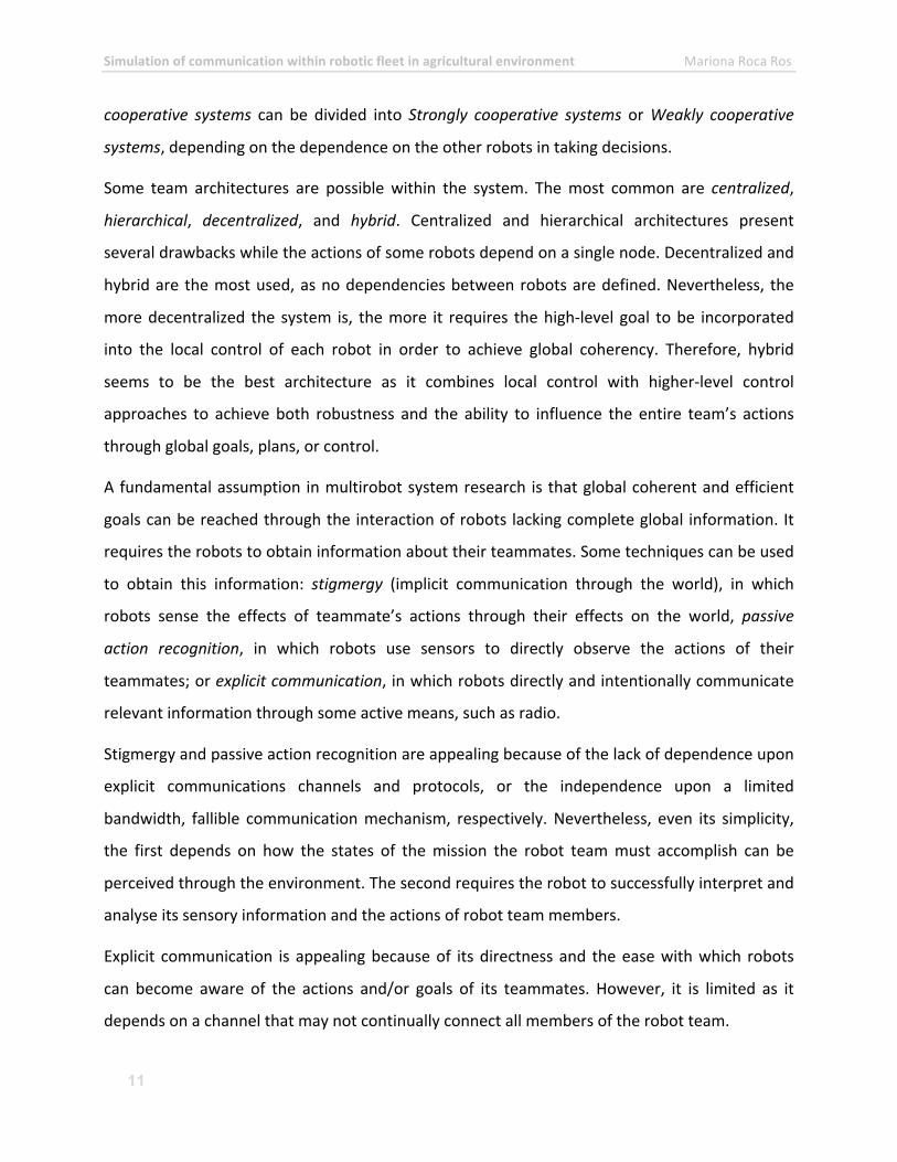
The RHEA mobile units include a High-‐level Decision Making System (HLDMS) which is in charge
of deciding what process to apply, where to apply it, the optimum dose and the application
instants. These basic functions make the HLDMS interact among the Mission Manager (MM),
the perception, the actuation and the location system.
Figure 1 depicts the logical position and relationships of the HLDMS with the rest of subsystems
in the overall RHEA system.
Figure 1 The logical position and relationships of the HLDMS with the rest of the subsystems
The inputs of the HLDMS are a local or total plan generated by the MM based on Mission field
dimensions and terrain irregularities, the previously knowledge on the crops and weeds of the
Simulation of communication within robotic fleet in agricultural environment Mariona Roca Ros
15
mission field, the commands from the user portable device, the data from the perception
system and the status from the ground mobile units (unit position, heading and speed).
To configure the HLDMS behaviour the solutions are different depending on the application
scenarios (narrow-‐row crop, wide-‐row crop and woody perennial).
As an example, the application in narrow-‐row crop is specified below so that it can be simulated
the most accurately as possible.
The narrow-‐row crop scenario for RHEA has been decided to be based on winter cereal (wheat)
and the mission consists of herbicide application with spray booms.
1. The operator starts up the system.
2. The operator defines the mission and provides the field features to the MM.
3. The MM orders a drone flying mission for taking crop images.
4. The remote perception system identifies the weed patches and types.
5. The MM computes a plan for each ground mobile unit.
6. The mission plan is sent to the HLDMS of the mobile units. This plan will be a table, each
entry containing: a point of the mobile unit trajectory and the speed to achieve that
point, and actions to be performed in that point.
7. The HLDMS can change the plan according to the information from the perception
system.
8. The HLDMS will report a ground mobile unit status to the MM.
The ground mobile units (GMU) will move over the crops by following two types of trajectories:
pre-‐defined tramlines or real-‐time computed paths. In any case, those trajectories will be
provided by the MM.
Simulation of communication within robotic fleet in agricultural environment Mariona Roca Ros
16
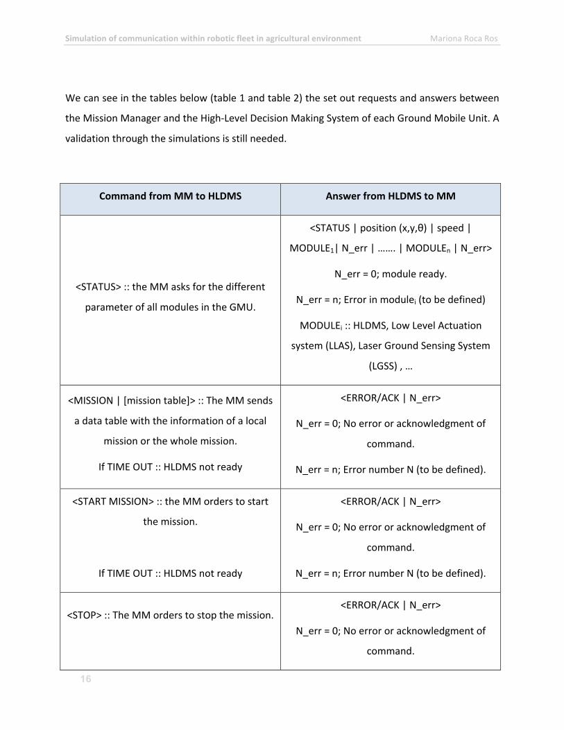
We can see in the tables below (table 1 and table 2) the set out requests and answers between
the Mission Manager and the High-‐Level Decision Making System of each Ground Mobile Unit. A
validation through the simulations is still needed.
Command from MM to HLDMS Answer from HLDMS to MM
<STATUS> :: the MM asks for the different
parameter of all modules in the GMU.
<STATUS | position (x,y,θ) | speed |
MODULE1| N_err | ……. | MODULEn | N_err>
N_err = 0; module ready.
N_err = n; Error in modulei (to be defined)
MODULEi :: HLDMS, Low Level Actuation
system (LLAS), Laser Ground Sensing System
(LGSS) , …
<MISSION | [mission table]> :: The MM sends
a data table with the information of a local
mission or the whole mission.
If TIME OUT :: HLDMS not ready
<ERROR/ACK | N_err>
N_err = 0; No error or acknowledgment of
command.
N_err = n; Error number N (to be defined).
<START MISSION> :: the MM orders to start
the mission.
If TIME OUT :: HLDMS not ready
<ERROR/ACK | N_err>
N_err = 0; No error or acknowledgment of
command.
N_err = n; Error number N (to be defined).
<STOP> :: The MM orders to stop the mission.
<ERROR/ACK | N_err>
N_err = 0; No error or acknowledgment of
command.
Simulation of communication within robotic fleet in agricultural environment Mariona Roca Ros
17
If TIME OUT :: HLDMS not ready N_err = n; Error number N (to be defined).
<CONTINUE> :: The MM orders to resume the
mission.
If TIME OUT :: HLDMS not ready
<ERROR/ACK | N_err>
N_err = 0; No error or acknowledgment of
command.
N_err = n; Error number N (to be defined).
<GOTO | x | y | θ | speed> :: MM command
to position the GMU in position (x,y) with
heading θ.
If TIME OUT :: HLDMS not ready
<ERROR/ACK | N_err>
N_err = 0; No error or acknowledgment of
command.
N_err = n; Error number N (to be defined).
<CONFIG> :: MM asks for the module and
subsystem configuration onboard the GMU.
<CONFIG | Module WDS | ·∙·∙·∙·∙·∙·∙·∙ | Module LGSS
| Tool>
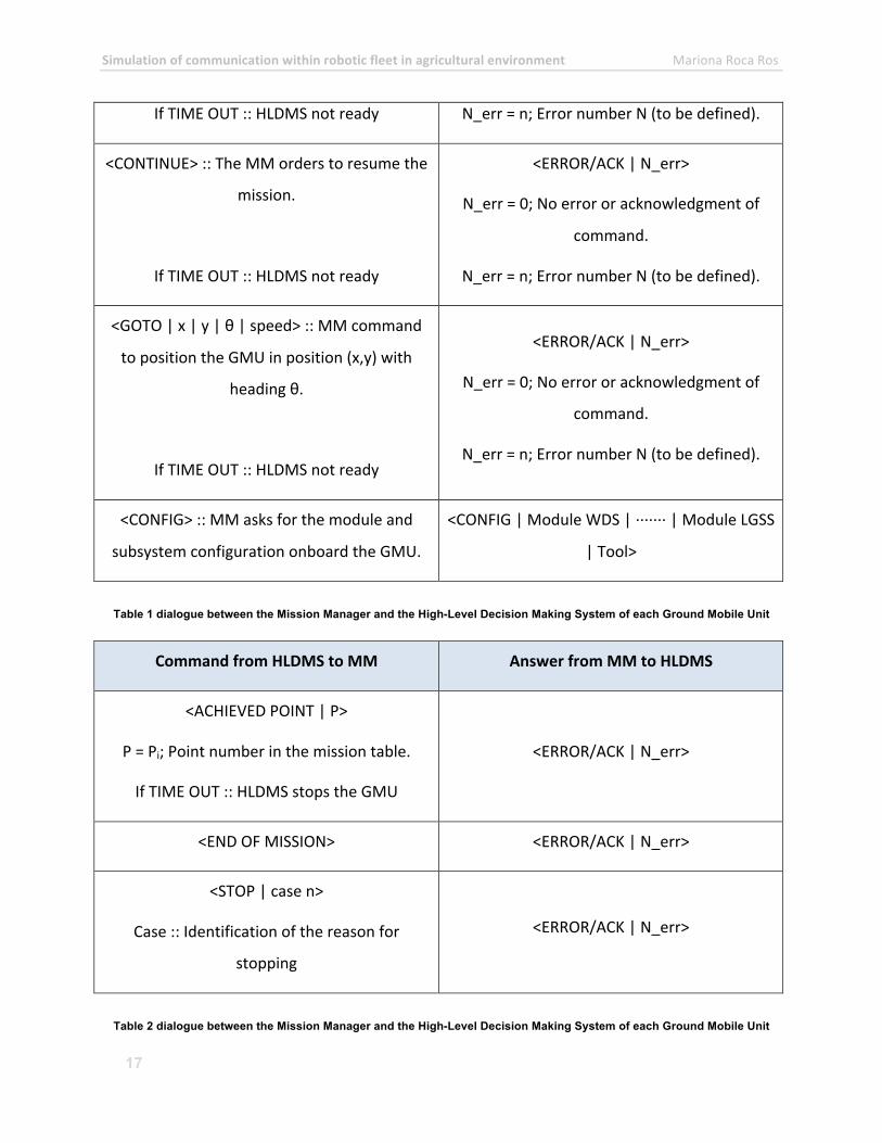
Table 1 dialogue between the Mission Manager and the High-Level Decision Making System of each Ground Mobile Unit
Command from HLDMS to MM Answer from MM to HLDMS
<ACHIEVED POINT | P>
P = Pi; Point number in the mission table.
If TIME OUT :: HLDMS stops the GMU
<ERROR/ACK | N_err>
<END OF MISSION> <ERROR/ACK | N_err>
<STOP | case n>
Case :: Identification of the reason for
stopping
<ERROR/ACK | N_err>
Table 2 dialogue between the Mission Manager and the High-Level Decision Making System of each Ground Mobile Unit
Simulation of communication within robotic fleet in agricultural environment Mariona Roca Ros
18
Even though there are also more specific commands to communicate the HLDMS with other
modules within the Ground Mobile Unit (the Ground Mobile Unit Controller, the Actuation
Controller, the Row and Obstacle Detection System…), we are just interested in the
communication between the Ground Mobile Unit and other robots, while it will be performed
through a wireless interface (either by using IEEE 802.11 a/g or IEEE 802.15.4 ZigBee standards).
In this thesis IEEE 802.11 will be implemented and assumed in all the simulations in realistic
RHEA scenarios, even though they are performed by using other wireless standards such as
ZigBee or an other version of 802.11.
The RHEA scenario implies the following specifications that will be taken into account in all the
simulations:
• Size of the field = 150 x 300 m2
• Robot speed = 5.5 Km/h
• Antenna height = 2.5 m
The number of robots in the simulations will change depending on the concrete scenario. In this
thesis the communication between the HLDMS of the GMU and the MM (a remote base station
allocated in a fixed point in the field) will be validated according to different used versions of
the Wireless standard (802.11a and g).
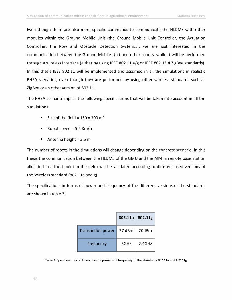
The specifications in terms of power and frequency of the different versions of the standards
are shown in table 3:
802.11a 802.11g
Transmition power 27 dBm 20dBm
Frequency 5GHz 2.4GHz
Table 3 Specifications of Transmission power and frequency of the standards 802.11a and 802.11g
Simulation of communication within robotic fleet in agricultural environment Mariona Roca Ros
19
1.2 Problem Statements
Before implementing any device in the RHEA robotic fleet, their response must be known and
controlled to respect the previous desired behaviour. Therefore, to check the range of
possibilities when using a communication standard, simulations are definitely needed.
Likewise, once the range of possibilities is tested and agrees with the expectations, the mission
planner will use the simulator to design the mission to be distributed among the robots.
Even though it already exists a simulation software package that allows the user to simulate the
behaviour of the robots, simulation of communication merely works at a physical level, and so,
it is not developed enough to be included in the simulations where communication is important.
In conclusion, the problem to be solved through this thesis is how to efficiently model the
communication at different levels in order to support mission planning, supervision and re-‐
planning – off-‐line and in the real time.
1.3 Outline of Thesis
Chapter 1 has presented a brief introduction to the state of the art and concepts related to the
main topic of this thesis: fleets of communicated robots and their applications, with special
focus on the RHEA project, where the development of this thesis is framed.
Chapter 2 presents the requirements and the performance criteria in the communication in
robotic fleets in agricultural environments. The communication technology implemented in the
simulations has also been explained in detail in this chapter.
Chapter 3 introduces the platform where simulations are performed (the Webots software) as
well as the already existing tool for network simulations in which we based to adapt to the
needs of the RHEA project the different algorithms. In this chapter the final simulated model is
also explained in detail.
Chapter 4 is based on the realization of the communication stack in Webots. The created
architecture is also explained in this chapter, but also the consequences of using a different type
of simulator for which the algorithms were defined, such as the time scaling.
Simulation of communication within robotic fleet in agricultural environment Mariona Roca Ros
20
New given functionalities are also specified in this section, like the new implemented
propagation models, the rebroadcast mechanism, the adaptation of the Webots’ Emitter node
to all the new needed parameters, or the metrics definition for the different types of packets.
Chapter 5 refers to the evaluation once the model is created. The performance criteria is
defined so that realistic scenarios can be defined and discussed. The way results of a simulation
are obtained is also explained in this chapter.
Chapter 6 presents the conclusions of this thesis, which was its contribution, and also reflect on
further extensions and new aspects to be considered in future work.
Chapter 7 shows the references used to the development of this thesis.
In the Appendixes, the most important implemented classes are defined in the first
section(Application, MAC, physical and prereceive layer, as well as the mobilerobot and the
scheduler).
The modification of the Webots emitter node is also shown in the second Appendix.
In the third one, the results of the simulations are explained in more detail. And finally, a user
manual is also attatched.
Simulation of communication within robotic fleet in agricultural environment Mariona Roca Ros
21
2. Communication in Robotic Fleets in Agriculture
2.1 Application of Robotic Fleets
As explained in previous sections, the developments done in this thesis are focused on an
already existing project oriented to enhance the efficiency of agriculture and forestry
management, RHEA (Robot Fleets for Highly Efficient Agriculture and Forestry Management).
The aim of this project is to minimize chemical product utilization, energy and time, and to
maximize the quality and safety of the products.
The robots are ruled by predefined mission description created according to the information
about the field, the agricultural tasks and capabilities of the robots. The process of creating this
mission includes the process of simulation.
After the mission is defined, the base station sends it to all the robots via wireless interfaces.
There is an continuous actively exchange of data between the base station and the robots, as
they will inform the mission supervisor about the state of the mission and receiving the actual
corrections of it.
It is important to maintain communication of sufficient quality within the fleet during the whole
mission, or alternatively, taking into account that wireless interfaces implemented on the robots
have some constraints in terms of bandwidth and coverage. Therefore, it is important to design
a mission in such a way that makes it possible to assure required quality of communications
within the fleet and among the robots and the base station.
2.2 Fleet Communication Requirements and Performance Criteria
The work of this thesis is to evaluate the possibility to use more realistic communication model
of the wireless interfaces when simulating the RHEA mission, to understand the possible gains
of this approach in the mission design.
The way we evaluate the performance through simulations is by analysing some parameters in
the obtained file at the end of the simulation.
Simulation of communication within robotic fleet in agricultural environment Mariona Roca Ros
22
To first check the correct performance of the 802.11 communication standard implementation,
the time, the type of packet (control or data packet) and the allocation (node and layer) at
which some events are produced, are evaluated.
The quality of the wireless communication between the different robots of each scenario is
checked through the analysis of the delay of a packet from the moment it is generated at the
emitter node to the moment at which it is completely received and processed by the application
layer of the receiver node.
As well, the packet loss rate is evaluated, and it is related to the distance between the robots.
This way, we can define the different range possibilities depending on the disposition of the
robots within the field, and on the different possible propagation models.
Basing on this checked parameters, some possible scenarios are evaluated, such as by using a
rebroadcast mechanism, using different propagation models, or adding metrics to the packets
so that priorities can be implemented.
Some definitions can be further introduced, as some other criteria can be used to check the
quality of the result performance of the simulations:
• Resilience: The ability to provide and maintain an acceptable level of service in the
face of faults and challenges to normal operation. In order to increase the resilience
of a communication network, the probable challenges and risks have to be identified
and appropriate resilience metrics have to be defined for the service to be protected.
• Synchronization: Timekeeping which requires the coordination of events to operate a
system in unison. Many services running on modern digital telecommunication
networks require accurate synchronization for correct operation. Therefore,
telecommunication networks rely on the use of highly accurate primary reference
Simulation of communication within robotic fleet in agricultural environment Mariona Roca Ros
23
clocks which are distributed network wide using synchronization links and
synchronization supply units.
• Mobility: The ability of a system to move and keep at the same time all the
functionalities it was designed and implemented for.
• Metrics: a property of a route in computer networking, consisting of any value used
by Routing Protocol to determine whether one route should perform better than
another. A metric can include measuring link utilisation, the number of hops, the
speed of the path, the router congestion, the latency, the path reliability, the
throughput...
2.3 OSI Model
The open system interconnection (OSI) is a descriptive network model created by the
International Organization for Standardization (ISO) in 1984. It defines a reference frame for the
definition of interconnection architectures in communication systems.
The base of this standard is the reference model OSI, a norm formed by seven layers that define
the different stages which data must pass through when travelling from one device to an other
in a communication network.
This model specifies the protocol to be use at each layer. It is a useful standardized norm that
creates a method in which all devices can understand each other someway, even when
technologies or brands don’t coincide. Therefore, the geographic allocation or the used
language is not important while the devices follow the norms to communicate among
themselves.
This model is divided into seven layers:
Physical layer: It manages the global connection of the computer to the network in the physical
media and the way information is transmitted.
Link layer: It manages the physical routing, the network topology, the media access, the error
detection, the frame distribution and the flow control.
Simulation of communication within robotic fleet in agricultural environment Mariona Roca Ros
24
Network layer: It identifies the existing routing between one or more networks. Its objective is
to make data arrive to the destination, even when both emitter and receiver are not directly
connected. The device that make it possible are called routers, and they work at this level.
Transport layer: it is in charge of transporting the data within the packet from the source to the
destination, independent of the physical network being used.
Session layer: it keeps and controls the established link between two computers transmitting
any kind of data.
Presentation layer: It is in charge of representing the information, so even different terminals
can have different inner representations of the characters, the data arrive in an identifiable way
to the destination.
Application layer: It offers the applications the possibility to accede to the services of the other
layers and it define the used protocols of the application to send and receive data, such as the
e-‐mail (Post Office Protocol and SMTP), file servers (FTP),...
2.4 Communication Technology -‐ WLAN
A wireless network is a data communication system that provides wireless connection between
the devices allocated within its area of coverage.
Instead of transmitting through a twisted pair, a coaxial cable or optical fibre, as used in
conventional LANs, wireless networks transmit and receive data through electromagnetic waves
using the air as transmission media.
Depending on its coverage area, wireless network can be divided in WPAN (Wireless Personal
Area Network), WLAN (Wireless Local Area Network), WWAN (Wireless Wide Area Network), ...
WLAN network is a Local Area Network. It can cover, inside a building, around 100 meters. It
allows the devices allocated inside the range of the network interconnect.
We can distinguish between different technologies for WLAN communication:
§ IEEE 802.11 with all its different versions.
§ ETSI Hiper LAN2 (High Performance Radio LAN 2.0)
Simulation of communication within robotic fleet in agricultural environment Mariona Roca Ros
25
• IEEE 802.11
The original 802.11 standard was developed in 1997 by IEEE (The Institute of Electrical and
Electronics Engineers). This base standard is still being enhanced through document additions
that are designated by a letter following the 802.11 name, such as 802.11b, 802.11a, or
802.11u. The letter suffix represents the task group that defines the extension to the standard.
These enhancements bring increases in data rate and functionality leading to rapid progression
of the WLAN.
In this thesis, 802.11a and 802.11g are mostly used.
IEEE 802.11a standard operates in the 5GHz spectrum. It was designed for higher bandwidth
application than previous versions (such as 802.11b), and includes rates of 6, 9, 12, 18, 24, 36,
48, and 54 Mbps using Orthogonal Frequency Division Multiplexing (OFMD) modulation on up
to 12 discrete channels. It has had a limited market acceptance primarily due to its lack of
backward compatibility with 802.11b products, shorter connectivity range, and higher
deployment costs.
IEEE 802.11g, in the other hand, was defined to work in the 2.4GHz unlicensed spectrum to data
rates faster than 20 Mbps, even it provides data rates of up to 54 Mbps, and requires backward
compatibility with 802.11b devices to protect the substantial investments in today’s WLAN
installations. It uses OFDM and CCK modulations.
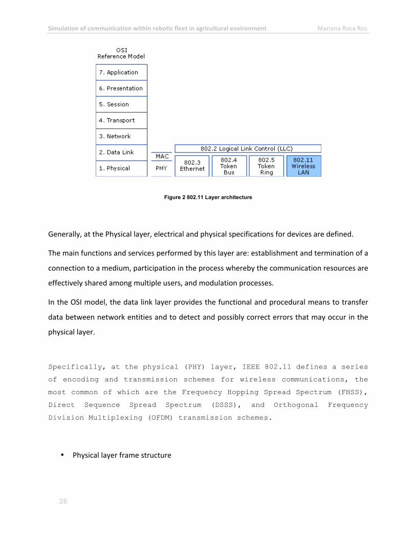
Picture 2 shows the 802.11 layer architecture.
As any 802.x protocol, it covers the MAC and the Physical layer (the two last levels of the OSI
architecture). It defines the technology of local area networks and metropolitan area networks.
Simulation of communication within robotic fleet in agricultural environment Mariona Roca Ros
26
Figure 2 802.11 Layer architecture
Generally, at the Physical layer, electrical and physical specifications for devices are defined.
The main functions and services performed by this layer are: establishment and termination of a
connection to a medium, participation in the process whereby the communication resources are
effectively shared among multiple users, and modulation processes.
In the OSI model, the data link layer provides the functional and procedural means to transfer
data between network entities and to detect and possibly correct errors that may occur in the
physical layer.
Specifically, at the physical (PHY) layer, IEEE 802.11 defines a series
of encoding and transmission schemes for wireless communications, the
most common of which are the Frequency Hopping Spread Spectrum (FHSS),
Direct Sequence Spread Spectrum (DSSS), and Orthogonal Frequency
Division Multiplexing (OFDM) transmission schemes.
• Physical layer frame structure
Simulation of communication within robotic fleet in agricultural environment Mariona Roca Ros
27
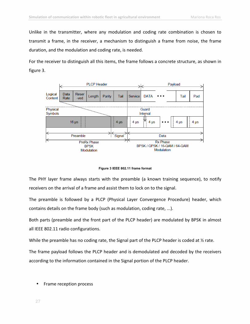
Unlike in the transmitter, where any modulation and coding rate combination is chosen to
transmit a frame, in the receiver, a mechanism to distinguish a frame from noise, the frame
duration, and the modulation and coding rate, is needed.
For the receiver to distinguish all this items, the frame follows a concrete structure, as shown in
figure 3.
Figure 3 IEEE 802.11 frame format
The PHY layer frame always starts with the preamble (a known training sequence), to notify
receivers on the arrival of a frame and assist them to lock on to the signal.
The preamble is followed by a PLCP (Physical Layer Convergence Procedure) header, which
contains details on the frame body (such as modulation, coding rate, ...).
Both parts (preamble and the front part of the PLCP header) are modulated by BPSK in almost
all IEEE 802.11 radio configurations.
While the preamble has no coding rate, the Signal part of the PLCP header is coded at ½ rate.
The frame payload follows the PLCP header and is demodulated and decoded by the receivers
according to the information contained in the Signal portion of the PLCP header.
• Frame reception process
Simulation of communication within robotic fleet in agricultural environment Mariona Roca Ros
28
In general, wireless radios are not able to send and receive data simultaneously in the same
channel. Therefore, a radio is always in one and only one of three conditions:
o Listening to the channel searching for new incoming frames to be received.
o Transmitting a frame (only when commanded by the MAC layer).
o Receiving (or at least attempting in) receiving a frame.
When listening to the channel, the radio continuously looks for the known pattern of the
preamble by demodulating the received signal according to BPSK demodulation method. If this
pattern is finally found, the receiver will attempt to decode the Signal portion of the PLCP
header. In case it is again successful, the receiver is then committed to demodulate the received
RF waveforms for the frame duration according to the information recovered in the Signal
portion of the PLCP header. From this point on to the end of the frame duration, the receiver
treats all received signal as belonging to the incoming frame and attempts to demodulate it. The
resulting row bits will be given to the MAC for CRC check to finally determine of a frame is
successfully received.
If a frame arrives when the node is transmitting, it will not detect this incoming signal as, at
least, it will have missed the critical preamble and PLCP part of the frame, and so, it will not be
able to receive it because of a lack of information.
Similarly, if a node is receiving frame it will not be able to receive a new incoming frame
because the node would treat the signal from the new frame as from the frame currently being
received (some possible exception to allow such a new frame to be received is possible).
In the case this new incoming frame has strong enough signal strength, it will collide with the
existing frame and prevents its successful reception.
Depending on the signal quality and on the interferences, it is possible for a node to have a
correct reception of the preamble and PLCP, but not to be able to correctly receive the frame
body.
Simulation of communication within robotic fleet in agricultural environment Mariona Roca Ros
29
• Benefits
The benefits of using the IEEE 802.11 standard are the advantages of using an already
developed and commercial standard. The cost of implementation is cheap, as it is a popular
device. It helps not having compatibility problems within the devices.
• Limitations
Actually, some limitations are present in the use of this standard, and must be properly solved.
The biggest problem when using IEEE 802.11 is the signal range within dense vegetation
environment. In most cases, communication cannot be possible because of the distance and the
attenuation of the vegetation between emitter and receiver.
An other important fact is that, even the communication is possible between emitter and
receiver, the signal strength is limited. Adding speed means having higher signal strength. That’s
the reason why RHEA combines 802.11g with 802.11a. Nevertheless, increasing signal strength
has a higher cost.
This limitations are a big drawback in the RHEA project. Therefore, ZigBee, an other technology,
is also being used to communicate the robots. This standard is specially used in low consume
digital radio communication, and it is based in the standard IEEE 802.15.4 of WPAN (Wireless
Personal Area Network). It provides safe communication and maximizes the batteries lifetime.
Nevertheless, it provides a low data rate (around 250Kbps).
So both standards (IEEE 802.15.4 and IEEE 802.11a/g) will be used in the communication within
the RHEA robotic fleet, depending on the requirements at each moment.
Simulation of communication within robotic fleet in agricultural environment Mariona Roca Ros
30
3. Simulation of Robotic Systems and Mobile Networks
3.1 Introduction
The robots of the RHEA robotic fleet operate according to a predefined mission description
which is created using the information about the field and information about the agricultural
tasks and capabilities of the robots. The mission is a product of the mission planning software
running on the base station being the main command centre for the robots. The process of
creating the mission also includes its simulation. The RHEA integrated simulator offers for the
mission planner a graphical interface that shows the movements of the robots in the field and
the tasks that they perform. After the mission is designed the base station distributes the
mission specifics to all the robots via wireless interfaces. During the mission the robots actively
exchange data with the base station informing the mission supervisor about the state of the
mission and receiving the actual corrections to it.
Accordingly, it is important to maintain communication of sufficient quality within the fleet
during the whole mission, or alternatively, taking into account that wireless interfaces
implemented on the robots have some constraints in terms of bandwidth and the coverage, it is
important to design a mission in such a way that makes it possible to assure required quality of
communications within the fleet and among the robots and the base station.
This work aims at evaluating the possibility to use more realistic communication model of the
wireless interfaces when simulating the RHEA mission, to understand the possible gains of this
approach in the mission design, and to test how long such simulations could take.
3.2 Existing Platforms
Webots is a mobile robot simulator (Cyberbotics), where the user can define a 3D virtual world
and within it, the mobile robots are defined. Each of them have some devices (added by the
user prior to the simulation start), such as GPS, any mobile scheme, camera, emitter, receiver...
these last two ones are important because they are the starting point of the work developed in
this thesis.
Simulation of communication within robotic fleet in agricultural environment Mariona Roca Ros
31
The communication between the emitter and receiver device in the Webots simulator is
performed just at the Physical layer. Therefore, the aim of this thesis is to develop new
functionalities to make this communication perform at higher layers, so communication
standards can be easily implemented and used in the simulations.
This mobile robot simulator is a time-‐based simulator. Each of the mobile robots in the 3D
virtual world is ruled by its own controller, programmed by the user. Each time a certain
function is called, all the parameters relative to the devices are updated, and the process waits
for all the other robots to reach this same function in their controllers. This is how time is
managed in this simulator.
In the other hand, an other simulator tool is used in this thesis to implement the communication
layers for IEEE 802.11. This other simulator is NS2 (Network Simulator 2). NS2 is an open source
network simulator that offers simulation models for a wide range of networks and routing
protocols in a structured way.
On the contrary to Webots, NS2 is an event-‐based simulator. The operation of this system is
represented as a chronological sequence of events. Each event occurs at a concrete instant of
time (this is how time evolves in this system), and implies a change of state in the system.
In this thesis, IEEE 802.11 (Wireless) has been implemented, as well as the basis from which new
standards can be developed just by adding the appropriate layers.
The algorithms designed for NS2 (Network Simulator 2) have been used as a basis of our
implementations.
3.3 Webots Simulation of robotic fleets
Webots is a software package used to model, program and simulate mobile robots.
Simulation of communication within robotic fleet in agricultural environment Mariona Roca Ros
32
This tool models a 3D virtual world with physical properties, and allows users to add to it
multiple models of simple passive/active mobile robots with a wide range of different
properties and characteristics chosen by the user, such as different locomotion schemes or
sensor and actuator devices. The user can program each robot individually and once simulated
and checked port the software to commercially available physical robotic platforms.
This software tool has been used by a great number of universities and research centres
worldwide. However, in the field of communications, some limitations exist while the
communication components – the emitter and the receiver device, model only a physical layer
communication, omitting more rigorous implementation of the upper layers standards.
This work is focused on modelling the upper communication layers needed to simulate IEEE
802.11a wireless local area network (WLAN) communication standard in the Webots tool, and
may be a basis to implement other standards, e.g. ZigBee, in the future.
As explained before, Webots is a time based simulation tool, while NS2 is an event based
simulator. When the Webots simulator runs, each of the modelled robots is launched as a
different process. In a synchronous mode all robots share the same virtual time, and so, can
interact among themselves: each robot process runs separately, but they synchronize when the
function wb_robot_step(TIME_STEP) is called.
This function makes also the simulator compute the values of all parameters of the virtual world
and all the devices and sensors of all the robots after the TIME_STEP milliseconds .
So in short, this function makes the virtual time of the simulation move forward one step of
time. This concept determines the way in which new functionalities can be added.
3.4 NS-‐2 Simulation of mobile networks
3.4.1 General Information
NS is an open-‐source network simulator based in discrete events, widely used in education and
research environments.
Simulation of communication within robotic fleet in agricultural environment Mariona Roca Ros
33
Its main use takes place in research of mobile ad-‐hoc networks. It provides substantial support
for simulation of TCP, routing, and multicast protocols over wired and wireless (local and
satellite) networks.
3.4.2 Simulation Models
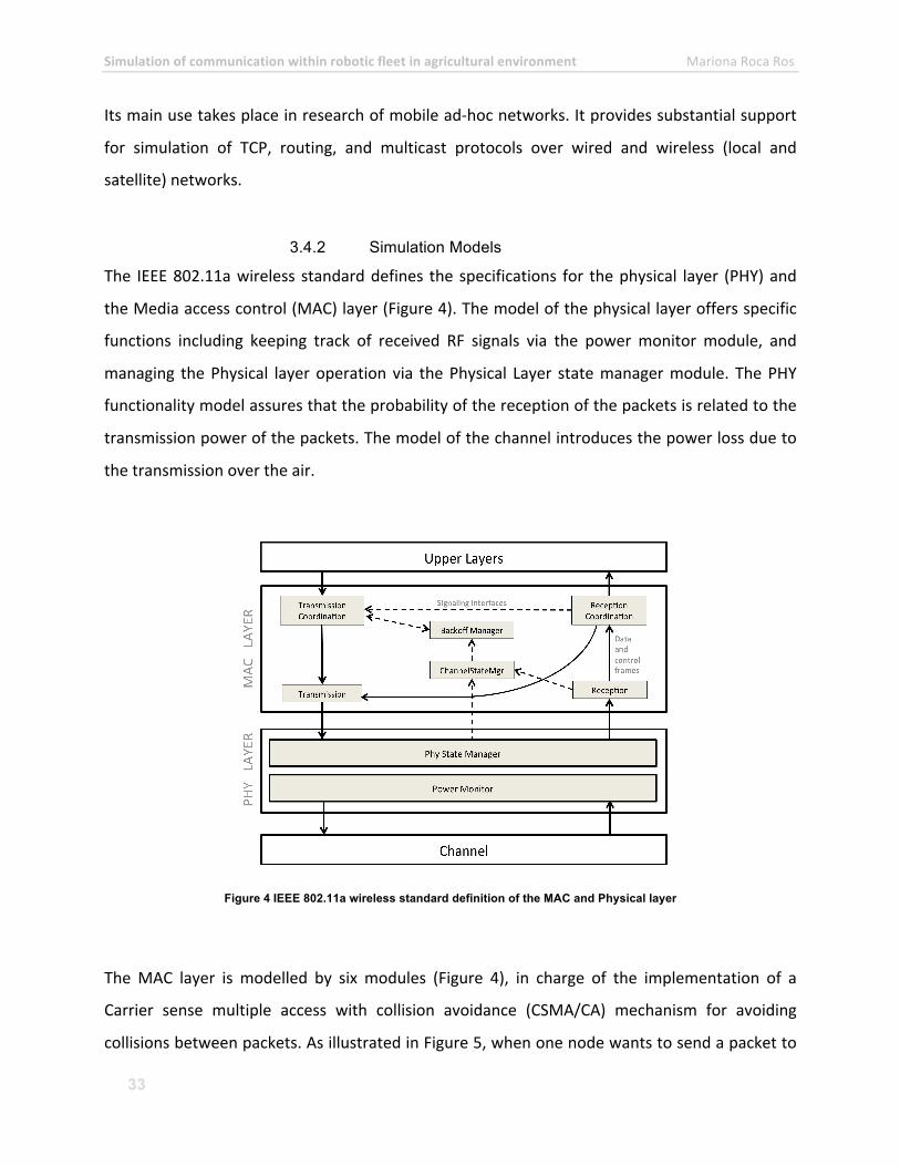
The IEEE 802.11a wireless standard defines the specifications for the physical layer (PHY) and
the Media access control (MAC) layer (Figure 4). The model of the physical layer offers specific
functions including keeping track of received RF signals via the power monitor module, and
managing the Physical layer operation via the Physical Layer state manager module. The PHY
functionality model assures that the probability of the reception of the packets is related to the
transmission power of the packets. The model of the channel introduces the power loss due to
the transmission over the air.
Figure 4 IEEE 802.11a wireless standard definition of the MAC and Physical layer
The MAC layer is modelled by six modules (Figure 4), in charge of the implementation of a
Carrier sense multiple access with collision avoidance (CSMA/CA) mechanism for avoiding
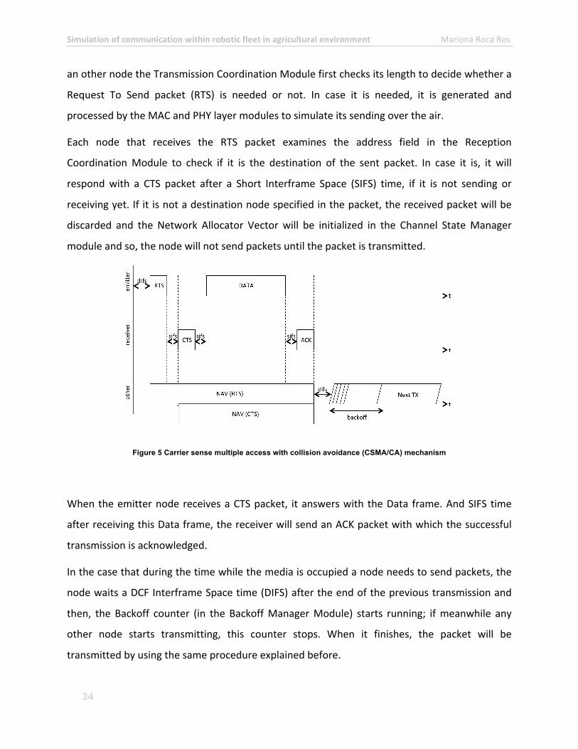
collisions between packets. As illustrated in Figure 5, when one node wants to send a packet to
Simulation of communication within robotic fleet in agricultural environment Mariona Roca Ros
34
an other node the Transmission Coordination Module first checks its length to decide whether a
Request To Send packet (RTS) is needed or not. In case it is needed, it is generated and
processed by the MAC and PHY layer modules to simulate its sending over the air.
Each node that receives the RTS packet examines the address field in the Reception
Coordination Module to check if it is the destination of the sent packet. In case it is, it will
respond with a CTS packet after a Short Interframe Space (SIFS) time, if it is not sending or
receiving yet. If it is not a destination node specified in the packet, the received packet will be
discarded and the Network Allocator Vector will be initialized in the Channel State Manager
module and so, the node will not send packets until the packet is transmitted.
Figure 5 Carrier sense multiple access with collision avoidance (CSMA/CA) mechanism
When the emitter node receives a CTS packet, it answers with the Data frame. And SIFS time
after receiving this Data frame, the receiver will send an ACK packet with which the successful
transmission is acknowledged.
In the case that during the time while the media is occupied a node needs to send packets, the
node waits a DCF Interframe Space time (DIFS) after the end of the previous transmission and
then, the Backoff counter (in the Backoff Manager Module) starts running; if meanwhile any
other node starts transmitting, this counter stops. When it finishes, the packet will be
transmitted by using the same procedure explained before.
Simulation of communication within robotic fleet in agricultural environment Mariona Roca Ros
35
In our simulation model the frames are generated in the application layer according to a data
generation rate, duration and size specified by the user before the simulation starts. This
information and other parameters relative to the simulation can be modified through the new
added fields of the Emitter node in Webots. Default values are provided. The application layer
schedules the first packet of the first flow, and the first packet of the other flows are stored in a
Queue List from where the MAC layer will pick the packets up when possible.
When a packet is received through the Webots emitter/receiver devices, it is sent to the
scheduler and when it is time to, it is attended by the physical layer according to the 802.11
protocol.
Simulation of communication within robotic fleet in agricultural environment Mariona Roca Ros
36
4. Realization of the Communication Stack in Webots
4.1 Architecture
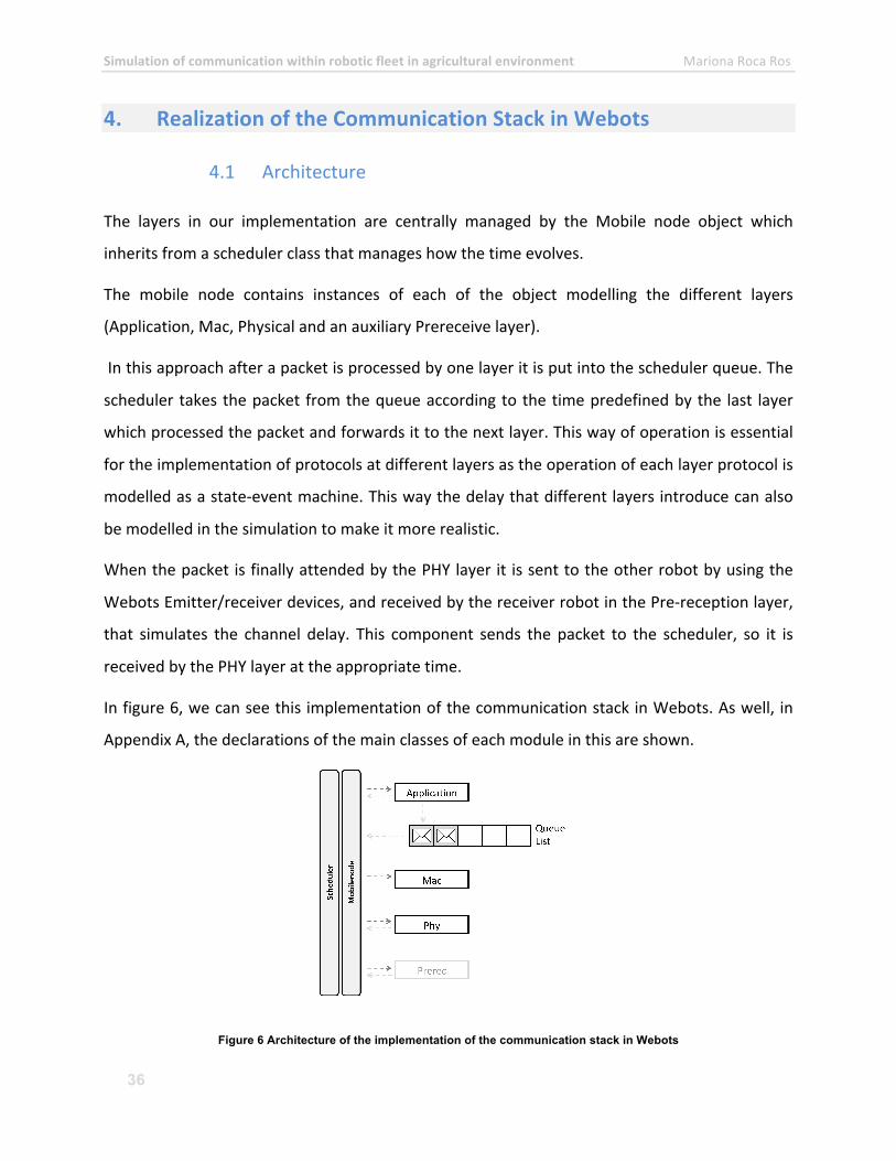
The layers in our implementation are centrally managed by the Mobile node object which
inherits from a scheduler class that manages how the time evolves.
The mobile node contains instances of each of the object modelling the different layers
(Application, Mac, Physical and an auxiliary Prereceive layer).
In this approach after a packet is processed by one layer it is put into the scheduler queue. The
scheduler takes the packet from the queue according to the time predefined by the last layer
which processed the packet and forwards it to the next layer. This way of operation is essential
for the implementation of protocols at different layers as the operation of each layer protocol is
modelled as a state-‐event machine. This way the delay that different layers introduce can also
be modelled in the simulation to make it more realistic.
When the packet is finally attended by the PHY layer it is sent to the other robot by using the
Webots Emitter/receiver devices, and received by the receiver robot in the Pre-‐reception layer,
that simulates the channel delay. This component sends the packet to the scheduler, so it is
received by the PHY layer at the appropriate time.
In figure 6, we can see this implementation of the communication stack in Webots. As well, in
Appendix A, the declarations of the main classes of each module in this are shown.
Figure 6 Architecture of the implementation of the communication stack in Webots
Simulation of communication within robotic fleet in agricultural environment Mariona Roca Ros
37
• Application layer
In the application layer, new packets are created according to the desired used application (by
now, just flows of data have been implemented). The user must specify through the Webots
interface the characteristics of the wanted flows of data in the simulations (starting time,
duration, speed, destination, modulation...).
• MAC layer
The MAC layer is based in the IEEE 802.11 MAC module designed for NS2 [12].
It is compounded by several objects modelling each of the sub modules ruled by state-‐event
machines, that allow the utilization of a CSMA/CA mechanism with the usage of Request-‐to-‐
send (RTS), clear-‐to-‐send (CTS) and Acknowledge (ACK).
Its structure is represented in the figure 7.
The Transmission Coordination Module manages channel access for the packets coming from
upper layer. It creates RTS when necessary and depending on the received packets it moves
from one state to the other (idle, RTS pending, wait RTS sent, wait CTS, wait SIFS, DATA pending,
wait PDU sent or wait ACK).
The Transmission Module is a simple state event machine with two states: Idle or Transmitting.
It sends the packets coming from the transmission coordination module to the scheduler. When
it is time to be attended, it will be sent by the mobile node to the lower layer. This way it is also
possible to take into account the delays in each of the layers in the simulation.
The Reception Coordination Module filters the packets to the upper layers and manages the
control packets. So in case a CTS or an ACK is received, it signals to the transmission
coordination module. It is also responsible of handling the CTS or ACK control packets when a
RTS or a unicast DATA packet arrives to the node. When it happens, it requests the Channel
State Manager for active Network Allocating Vector (NAV) in the node. In case there is an active
NAV, the packets that were going to be sent, will be immediately discarded. Otherwise, the
Simulation of communication within robotic fleet in agricultural environment Mariona Roca Ros
38
packet will be sent to the scheduler so it will be attended by the upper layer at the appropriate
time, according to the delay of the MAC layer.
The Reception Module is responsible of filtering and discarding packets which have an error (by
performing a CRC check), or which are not for the node. Before discarding a RTS or a CTS, it will
also check if a NAV is contained in the packet. If so, it will notify its value to the Channel state
Manager. It also signals to the Channel State Manager with virtual carrier sense updates. When
a packet arrives from the lower layer (through the scheduler), it will send the packet to the
reception coordination module.
The Channel State Manager is responsible of maintaining both the physical and the virtual
carrier sense statuses for the IEEE 802.11 mechanism. It expects the Physical layer to signal if
the channel is idle or busy. It also expects from the reception module to be informed of the
carrier sense updates so it will be able to set or update the NAV value for the specified duration.
The Channel State Manager will signal the state of the Carrier Sense to the Backoff Manager.
When it is at the state of “No CS no NAV”, it will signal “Carrier Sense Idle”. Otherwise, when it
is at the states of “CS no Nav”, “no CS NAV”, “CS NAV”, “WIFS”, it will signal “Carrier Sense
Busy”. This way, the Backoff manager will be able to pause or resume its Backoff process (if
there is already one).
The Backoff Manager maintains the Backoff counter to support the collision avoidance
mechanism. It has just three states: “No Backoff”, “Backoff running” and “Backoff pause”. The
state will depend on the signal received from the Channel State Manager.
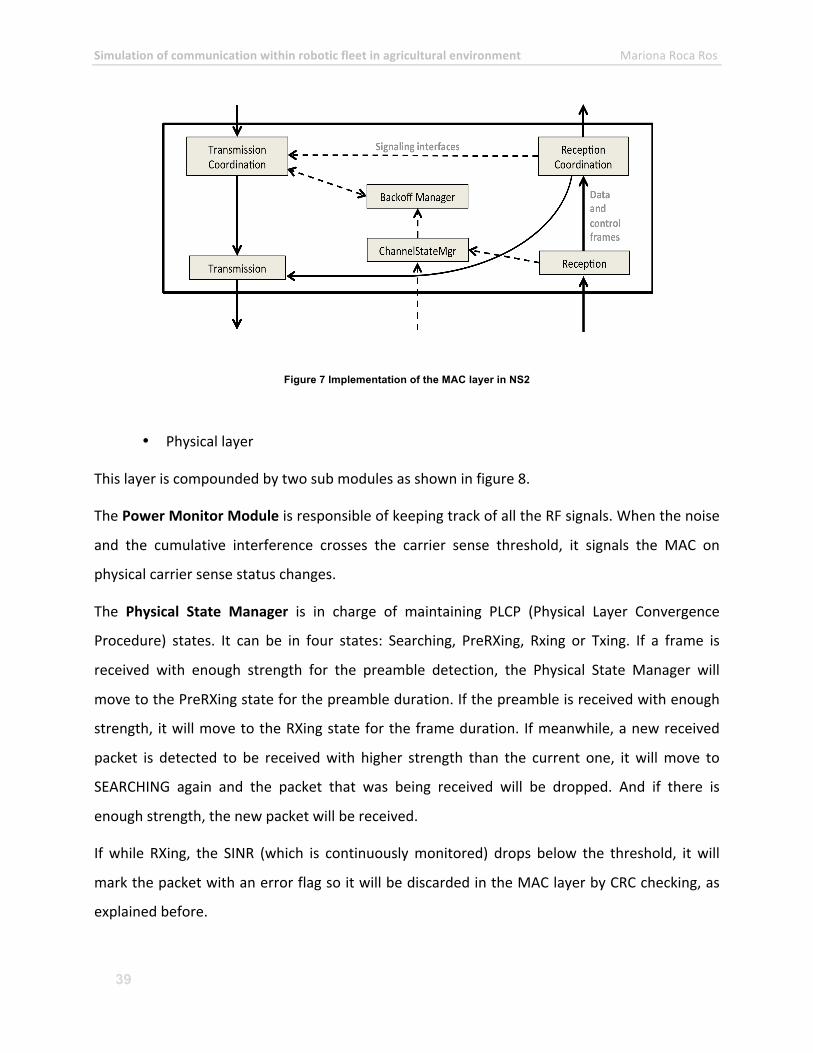
Simulation of communication within robotic fleet in agricultural environment Mariona Roca Ros
39
Figure 7 Implementation of the MAC layer in NS2
• Physical layer
This layer is compounded by two sub modules as shown in figure 8.
The Power Monitor Module is responsible of keeping track of all the RF signals. When the noise
and the cumulative interference crosses the carrier sense threshold, it signals the MAC on
physical carrier sense status changes.
The Physical State Manager is in charge of maintaining PLCP (Physical Layer Convergence
Procedure) states. It can be in four states: Searching, PreRXing, Rxing or Txing. If a frame is
received with enough strength for the preamble detection, the Physical State Manager will
move to the PreRXing state for the preamble duration. If the preamble is received with enough
strength, it will move to the RXing state for the frame duration. If meanwhile, a new received
packet is detected to be received with higher strength than the current one, it will move to
SEARCHING again and the packet that was being received will be dropped. And if there is
enough strength, the new packet will be received.
If while RXing, the SINR (which is continuously monitored) drops below the threshold, it will
mark the packet with an error flag so it will be discarded in the MAC layer by CRC checking, as
explained before.
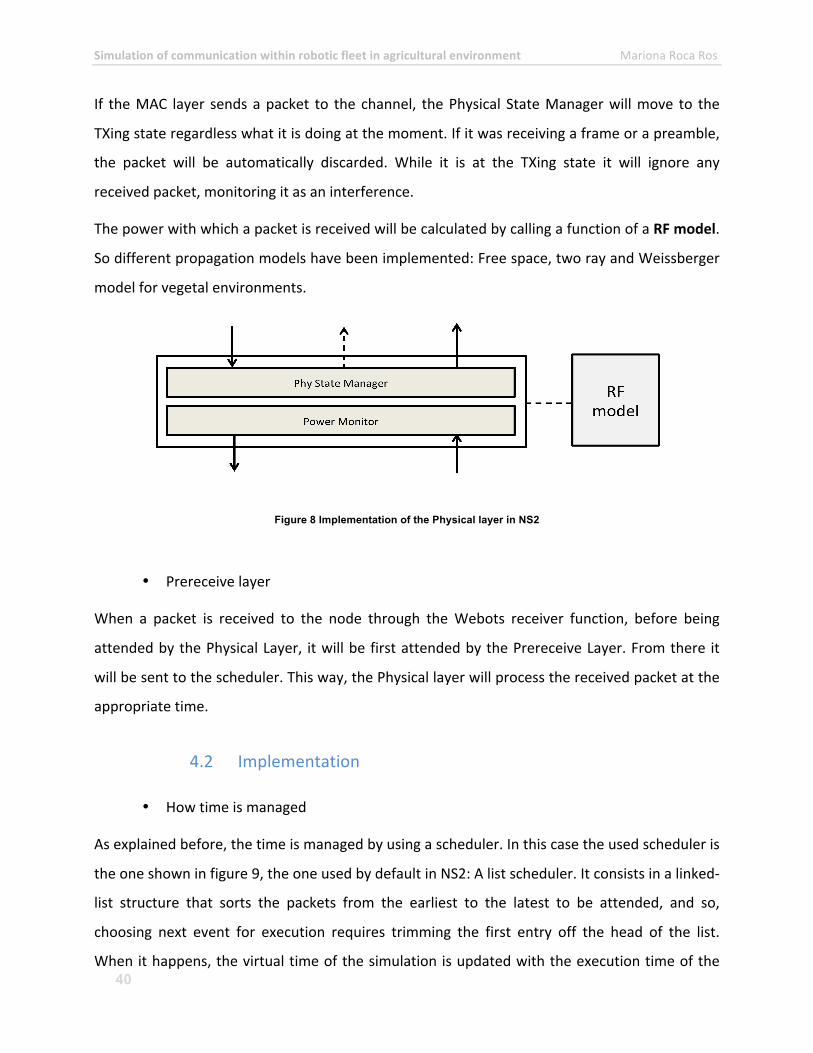
Simulation of communication within robotic fleet in agricultural environment Mariona Roca Ros
40
If the MAC layer sends a packet to the channel, the Physical State Manager will move to the
TXing state regardless what it is doing at the moment. If it was receiving a frame or a preamble,
the packet will be automatically discarded. While it is at the TXing state it will ignore any
received packet, monitoring it as an interference.
The power with which a packet is received will be calculated by calling a function of a RF model.
So different propagation models have been implemented: Free space, two ray and Weissberger
model for vegetal environments.
Figure 8 Implementation of the Physical layer in NS2
• Prereceive layer
When a packet is received to the node through the Webots receiver function, before being
attended by the Physical Layer, it will be first attended by the Prereceive Layer. From there it
will be sent to the scheduler. This way, the Physical layer will process the received packet at the
appropriate time.
4.2 Implementation
• How time is managed
As explained before, the time is managed by using a scheduler. In this case the used scheduler is
the one shown in figure 9, the one used by default in NS2: A list scheduler. It consists in a linked-‐
list structure that sorts the packets from the earliest to the latest to be attended, and so,
choosing next event for execution requires trimming the first entry off the head of the list.
When it happens, the virtual time of the simulation is updated with the execution time of the
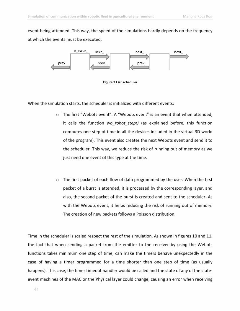
Simulation of communication within robotic fleet in agricultural environment Mariona Roca Ros
41
event being attended. This way, the speed of the simulations hardly depends on the frequency
at which the events must be executed.
Figure 9 List scheduler
When the simulation starts, the scheduler is initialized with different events:
o The first “Webots event”. A “Webots event” is an event that when attended,
it calls the function wb_robot_step() (as explained before, this function
computes one step of time in all the devices included in the virtual 3D world
of the program). This event also creates the next Webots event and send it to
the scheduler. This way, we reduce the risk of running out of memory as we
just need one event of this type at the time.
o The first packet of each flow of data programmed by the user. When the first
packet of a burst is attended, it is processed by the corresponding layer, and
also, the second packet of the burst is created and sent to the scheduler. As
with the Webots event, it helps reducing the risk of running out of memory.
The creation of new packets follows a Poisson distribution.
Time in the scheduler is scaled respect the rest of the simulation. As shown in figures 10 and 11,
the fact that when sending a packet from the emitter to the receiver by using the Webots
functions takes minimum one step of time, can make the timers behave unexpectedly in the
case of having a timer programmed for a time shorter than one step of time (as usually
happens). This case, the timer timeout handler would be called and the state of any of the state-‐
event machines of the MAC or the Physical layer could change, causing an error when receiving
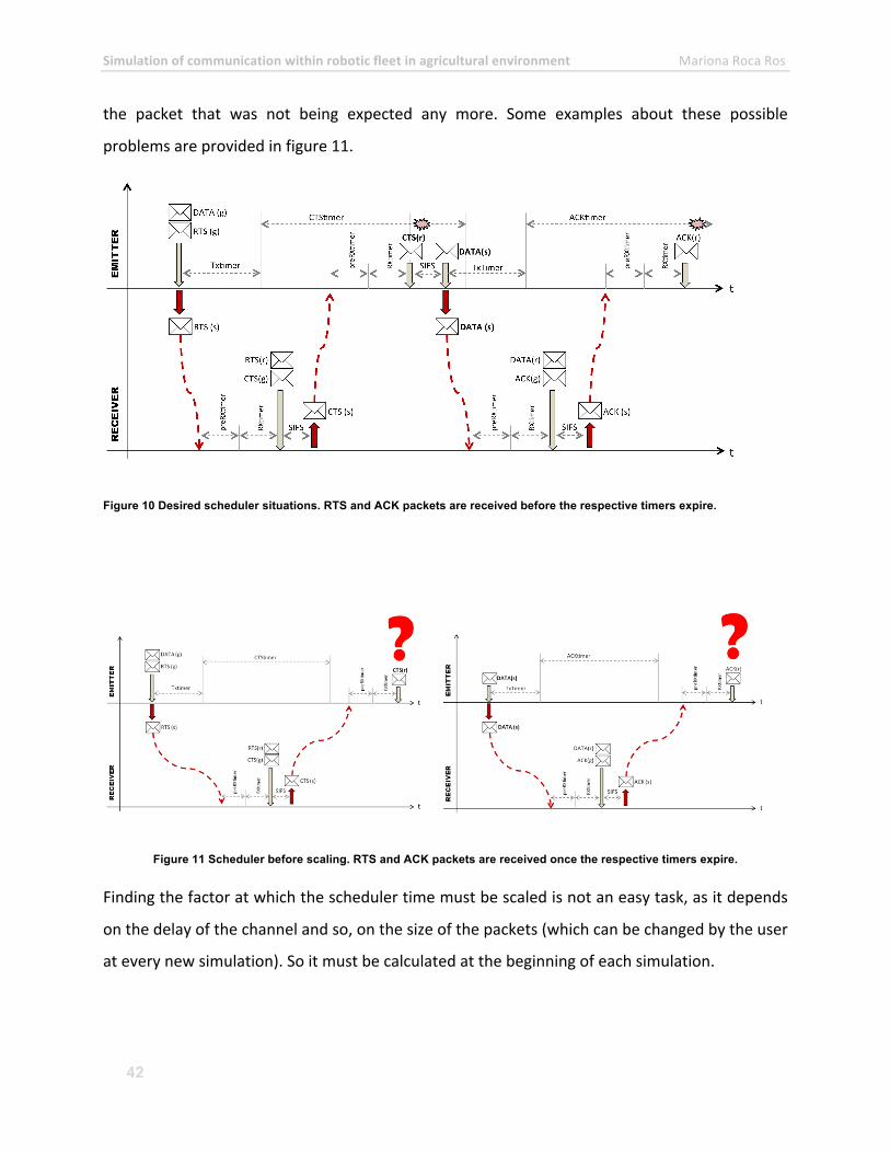
Simulation of communication within robotic fleet in agricultural environment Mariona Roca Ros
42
the packet that was not being expected any more. Some examples about these possible
problems are provided in figure 11.
Figure 10 Desired scheduler situations. RTS and ACK packets are received before the respective timers expire.
Figure 11 Scheduler before scaling. RTS and ACK packets are received once the respective timers expire.
Finding the factor at which the scheduler time must be scaled is not an easy task, as it depends
on the delay of the channel and so, on the size of the packets (which can be changed by the user
at every new simulation). So it must be calculated at the beginning of each simulation.
Simulation of communication within robotic fleet in agricultural environment Mariona Roca Ros
43
We can find an expression to calculate this factor by having a look at figure 10. The two possible
situations where the state conflict can arise are the one represented in figure 11. Keeping the
proportion between the time CTStimer and ACKtimer finish and the time CTS and ACK are
received, respectively, we arrive to the following expressions:
]_·2)··[()·( STEPTIMESTXtimerSIFSTXtimerKCTStimerTXtimerS RTSCTSRTSRTSRTSRTS +++=+
]_·2)··[()·( STEPTIMESTXtimerSIFSTXtimerKACKtimerTXtimerS ACKACKDATACKDATACK +++=+
{ }ACKRTS SSMAXS ,=
Where SRTS is the scale factor calculated through the situation of sending a RTS and receiving a
CTS, and SACK, the scale factor calculated through the situation of sending a DATA packet and
receiving an ACK.
KRTS and KACK are the proportion factor of the first and the second situation, respectively.
CTStimer and ACKtimer depend on the SIFS value, an additional maximum delay due to DSSS
and the CTS and ACK length respectively. As the simulator is provided with the values of these
lengths, we assume now the CTStimer and the ACKtimer to be fixed values.
SIFS value is also considered to be a fixed value even the user could change it through the
Webots interface. So when it is changed, it should be taken into account when recalculating the
scale factor of the scheduler.
TXtimer depends on the length of the packet. So, as we consider CTS and ACK to have a fixed
length, txtimer(CTS) and txtimer(ACK) will not change its value. But TXtimerDAT will depend on
the application that generates the packet.
In the simulations we run, we consider the RTS to have a lower length than the DATA packet, so
we assume the first equation to be more restrictive, and so, as it will give us the maximum scale
factor with these assumptions, we assume S = SRTS, following the expression:
Simulation of communication within robotic fleet in agricultural environment Mariona Roca Ros
44
]_·2)··[()·( STEPTIMESTXtimerSIFSTXtimerKCTStimerTXtimerS CTSRTSRTSRTS +++=+
So having a look at this, we have a compromise between two parameters: the scale factor (S)
and the step of time (TIME_STEP).
If a small step of time is chosen, the scale factor will be small, but the parameters of the
simulation will be recalculated frequently with the possibility of adding an extra computation
load to the program.
In the other hand, if a big step of time is chosen, the parameters of the simulations will be
recalculated with a lower frequency, but the scale of the time in the scheduler will be so big and
it will require more time to simulate a period of time in the communication.
The user must take into account the frequency of the events of the simulation and the amount
of time to simulate.
In the simulations performed in this thesis, a scale factor of 6500 has been introduced. It
corresponds with the minimum TIME_STEP (1 msec), as we expected having high rates of packet
generation and so, a high number of scheduled events.
• Adaptation of the emitter node in Webots
In order to get all the parameters from the user, the emitter node, initially provided by
Cyberbotics with fields just concerning to the physical layer, has been modified.
These modifications make the parameter introduction by the user easier.
All the nodes are specified in the folder /Webots/resources/nodes, and are text files with the
extension *.wrl.
When functionalities developed in this thesis are going to be used, the user will have to adapt
the ‘emitter.wrl’ file and overwrite it with the modifications. These modifications are specified
in the Appendix B of this thesis.
Simulation of communication within robotic fleet in agricultural environment Mariona Roca Ros
45
The delay of the different layers, the specification of the flows of data or the parameters
relative to the 802.11 (transmitted power, thresholds...) are some examples of the fields that
have been added to the node.
When the simulation starts, the controller of each robot catches all the values introduced in the
nodes by the user (default values are also provided for 802.11a) and assigns its values at his own
variables.
In the Appendix D, there is also a user manual that will help new users to start a simulation, and
where all the fields are also explained.
• Propagation models
Different propagation models have been provided within the developed new functionalities.
The propagation models are introduced at the Physical layer, so when a packet arrives from the
channel, through the functions provided by each model, the received strength can be checked.
Depending on the strength of the received packet, it will be considered to contain errors or not.
So it is important, for the reliability of the simulations, to have an appropriate propagation
model for each simulation, as the propagation will hardly depend on the type of crops present
at the field.
To determine which are the appropriate propagation models we will first explain which type of
propagation models we have and which could be suitable for RHEA simulation scenarios.
Basically, propagation models can be classified into deterministic model or probabilistic model.
Deterministic model: In this model, the received signal power is calculated according to some
parameters such as the distance between the emitter and the receiver. Some deterministic
models are:
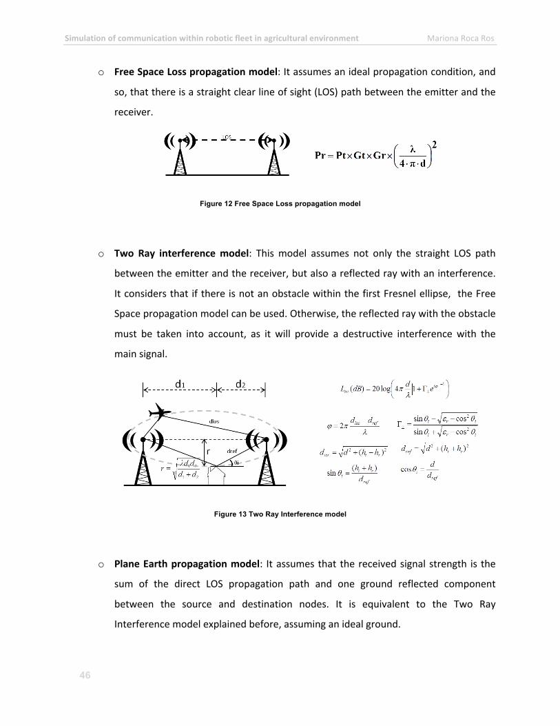
Simulation of communication within robotic fleet in agricultural environment Mariona Roca Ros
46
o Free Space Loss propagation model: It assumes an ideal propagation condition, and
so, that there is a straight clear line of sight (LOS) path between the emitter and the
receiver.
Figure 12 Free Space Loss propagation model
o Two Ray interference model: This model assumes not only the straight LOS path
between the emitter and the receiver, but also a reflected ray with an interference.
It considers that if there is not an obstacle within the first Fresnel ellipse, the Free
Space propagation model can be used. Otherwise, the reflected ray with the obstacle
must be taken into account, as it will provide a destructive interference with the
main signal.
Figure 13 Two Ray Interference model
o Plane Earth propagation model: It assumes that the received signal strength is the
sum of the direct LOS propagation path and one ground reflected component
between the source and destination nodes. It is equivalent to the Two Ray
Interference model explained before, assuming an ideal ground.
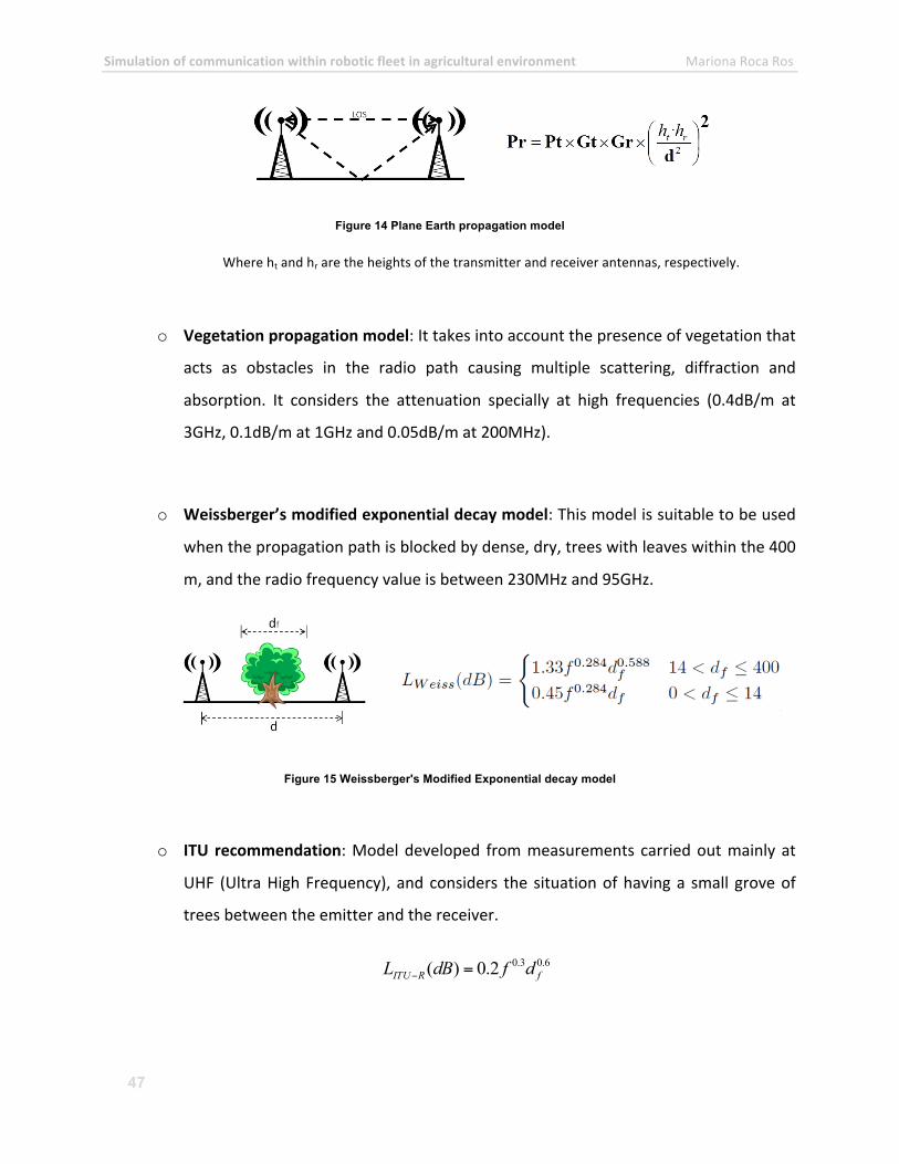
Simulation of communication within robotic fleet in agricultural environment Mariona Roca Ros
47
Figure 14 Plane Earth propagation model
Where ht and hr are the heights of the transmitter and receiver antennas, respectively.
o Vegetation propagation model: It takes into account the presence of vegetation that
acts as obstacles in the radio path causing multiple scattering, diffraction and
absorption. It considers the attenuation specially at high frequencies (0.4dB/m at
3GHz, 0.1dB/m at 1GHz and 0.05dB/m at 200MHz).
o Weissberger’s modified exponential decay model: This model is suitable to be used
when the propagation path is blocked by dense, dry, trees with leaves within the 400
m, and the radio frequency value is between 230MHz and 95GHz.
Figure 15 Weissberger's Modified Exponential decay model
o ITU recommendation: Model developed from measurements carried out mainly at
UHF (Ultra High Frequency), and considers the situation of having a small grove of
trees between the emitter and the receiver.
6.03.02.0)( fRITU dfdBL =−
Simulation of communication within robotic fleet in agricultural environment Mariona Roca Ros
48
Probabilistic model: As in most of the environments propagation loss is dynamic, it can be
characterized statistically. Therefore, probabilistic models allow a more realistic modelling of
radio wave propagation.
o Log-‐Normal shadowing: Shadowing occurs when objects block LOS between
transmitter and receiver. This method assumes that the average received signal
strength decreases logarithmically with distance. It uses a normal distribution with a
tabled variance to distribute receive power in the logarithmic domain.
o Rayleigh distribution: It is a fading model that describe the time-‐correlation of the
received signal strength. This propagation model represent situation with non Line of
Sight (NLOS) and only scattered components exist. This model shows intensive
variations in received signal strength because the scattered signal components can
either combine constructively or destructively.
The effects of the inclemency of the weather has been disregarded, as the attenuation in clear
weather, rain, fog and clouds is imperceptible at the range of frequencies we are working in.
In RHEA, the propagation is affected by vegetation (tomato, maize, strawberry, sunflower,
cotton, wheat, barley, walnut trees, almond trees, olive trees... ). Therefore, the models
implemented in this thesis are related to them. Due to the impossibility of developing and/or
implementing a model for all the possible crop, three propagation models have been
implemented:
• Free Space propagation model, to consider the ideal propagation condition.
• Two Ray Interference model, considering the scenario where the crop has not grown
yet, and the floor is wet.
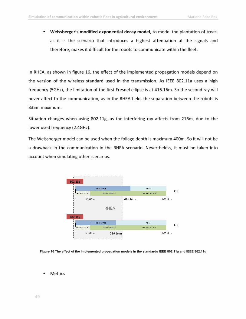
Simulation of communication within robotic fleet in agricultural environment Mariona Roca Ros
49
• Weissberger’s modified exponential decay model, to model the plantation of trees,
as it is the scenario that introduces a highest attenuation at the signals and
therefore, makes it difficult for the robots to communicate within the fleet.
In RHEA, as shown in figure 16, the effect of the implemented propagation models depend on
the version of the wireless standard used in the transmission. As IEEE 802.11a uses a high
frequency (5GHz), the limitation of the first Fresnel ellipse is at 416.16m. So the second ray will
never affect to the communication, as in the RHEA field, the separation between the robots is
335m maximum.
Situation changes when using 802.11g, as the interfering ray affects from 216m, due to the
lower used frequency (2.4GHz).
The Weissberger model can be used when the foliage depth is maximum 400m. So it will not be
a drawback in the communication in the RHEA scenario. Nevertheless, it must be taken into
account when simulating other scenarios.
Figure 16 The effect of the implemented propagation models in the standards IEEE 802.11a and IEEE 802.11g
• Metrics
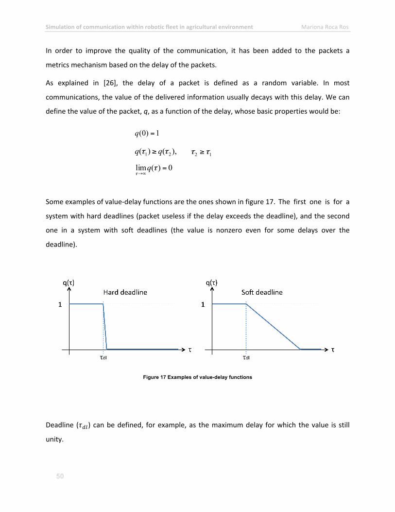
Simulation of communication within robotic fleet in agricultural environment Mariona Roca Ros
50
In order to improve the quality of the communication, it has been added to the packets a
metrics mechanism based on the delay of the packets.
As explained in [26], the delay of a packet is defined as a random variable. In most
communications, the value of the delivered information usually decays with this delay. We can
define the value of the packet, q, as a function of the delay, whose basic properties would be:
Some examples of value-‐delay functions are the ones shown in figure 17. The first one is for a
system with hard deadlines (packet useless if the delay exceeds the deadline), and the second
one in a system with soft deadlines (the value is nonzero even for some delays over the
deadline).
Figure 17 Examples of value-delay functions
Deadline (𝜏!") can be defined, for example, as the maximum delay for which the value is still
unity.
1)0( =q
),()( 21 ττ qq ≥ 12 ττ ≥
0)(lim =∞→
ττq
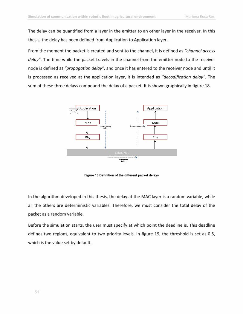
Simulation of communication within robotic fleet in agricultural environment Mariona Roca Ros
51
The delay can be quantified from a layer in the emitter to an other layer in the receiver. In this
thesis, the delay has been defined from Application to Application layer.
From the moment the packet is created and sent to the channel, it is defined as “channel access
delay”. The time while the packet travels in the channel from the emitter node to the receiver
node is defined as “propagation delay”, and once it has entered to the receiver node and until it
is processed as received at the application layer, it is intended as “decodification delay”. The
sum of these three delays compound the delay of a packet. It is shown graphically in figure 18.
Figure 18 Definition of the different packet delays
In the algorithm developed in this thesis, the delay at the MAC layer is a random variable, while
all the others are deterministic variables. Therefore, we must consider the total delay of the
packet as a random variable.
Before the simulation starts, the user must specify at which point the deadline is. This deadline
defines two regions, equivalent to two priority levels. In figure 19, the threshold is set as 0.5,
which is the value set by default.
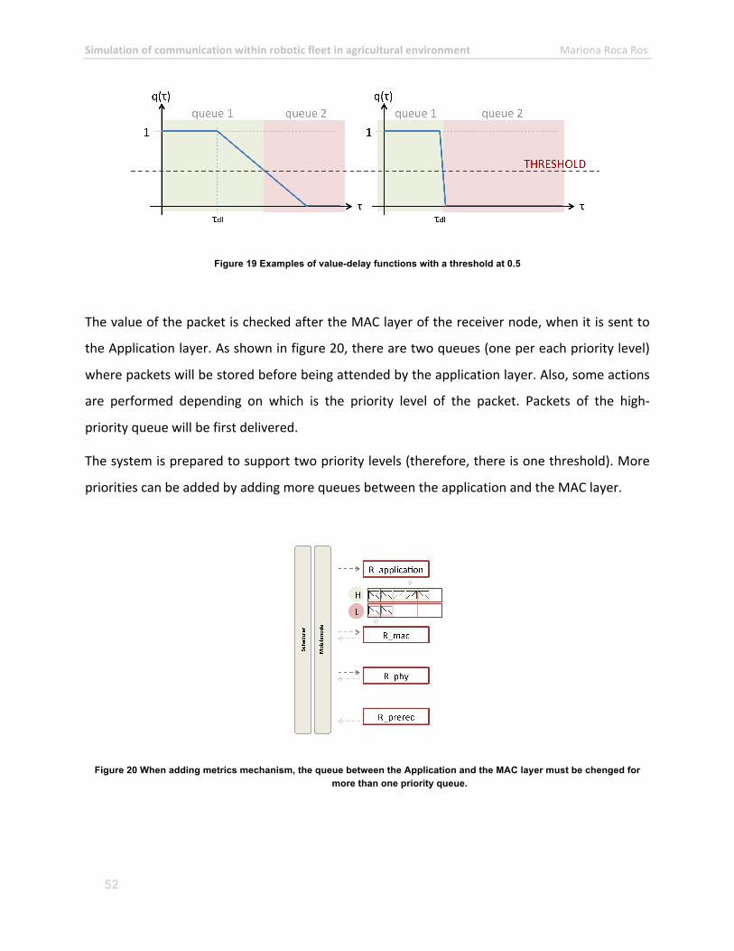
Simulation of communication within robotic fleet in agricultural environment Mariona Roca Ros
52
Figure 19 Examples of value-delay functions with a threshold at 0.5
The value of the packet is checked after the MAC layer of the receiver node, when it is sent to
the Application layer. As shown in figure 20, there are two queues (one per each priority level)
where packets will be stored before being attended by the application layer. Also, some actions
are performed depending on which is the priority level of the packet. Packets of the high-‐
priority queue will be first delivered.
The system is prepared to support two priority levels (therefore, there is one threshold). More
priorities can be added by adding more queues between the application and the MAC layer.
Figure 20 When adding metrics mechanism, the queue between the Application and the MAC layer must be chenged for more than one priority queue.
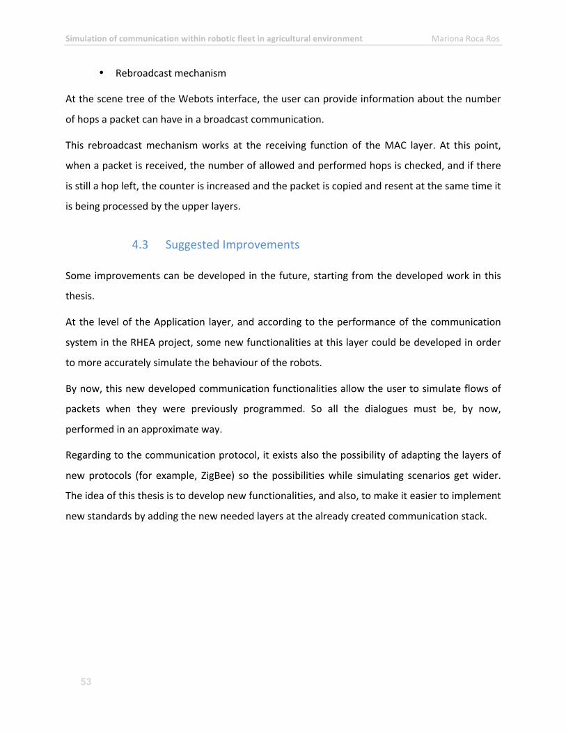
Simulation of communication within robotic fleet in agricultural environment Mariona Roca Ros
53
• Rebroadcast mechanism
At the scene tree of the Webots interface, the user can provide information about the number
of hops a packet can have in a broadcast communication.
This rebroadcast mechanism works at the receiving function of the MAC layer. At this point,
when a packet is received, the number of allowed and performed hops is checked, and if there
is still a hop left, the counter is increased and the packet is copied and resent at the same time it
is being processed by the upper layers.
4.3 Suggested Improvements
Some improvements can be developed in the future, starting from the developed work in this
thesis.
At the level of the Application layer, and according to the performance of the communication
system in the RHEA project, some new functionalities at this layer could be developed in order
to more accurately simulate the behaviour of the robots.
By now, this new developed communication functionalities allow the user to simulate flows of
packets when they were previously programmed. So all the dialogues must be, by now,
performed in an approximate way.
Regarding to the communication protocol, it exists also the possibility of adapting the layers of
new protocols (for example, ZigBee) so the possibilities while simulating scenarios get wider.
The idea of this thesis is to develop new functionalities, and also, to make it easier to implement
new standards by adding the new needed layers at the already created communication stack.
Simulation of communication within robotic fleet in agricultural environment Mariona Roca Ros
54
5. Evaluation
5.1 Performance Criteria
Before running the simulations, some criteria is defined to check the quality of the
communication.
The first run simulations are done to check the correct performance of the algorithms of the
new functionalities added to the simulator. We pay most of our attention to the delays of the
packets when passing from one layer to the following one, and to the correct sequence of
packets (specially when having control packets).
After checking the correct behaviour of the simulator, we pay special attention to the different
events (generation, sending, reception, discarding or rebroadcasting of packets) in order to
check the quality of the link in the different recreated scenarios.
The delay of the packets (from the moment they were created until the moment each event
finally happens) are also taken into special account. Specially at the scenarios where different
metrics were added to the packets.
The layer at which the different events are performed are also studied in order to check the
correct behaviour of the simulator.
In case of dropping a packet, the reason for which it was dropped is also being checked at the
point of logging all the events.
5.2 Simulation Scenarios
To evaluate the performance and the configuration of the RHEA robotic fleet in the fields, some
scenarios are defined, simulated and analyzed in this thesis.
• Propagation models
As different propagation models can be used, we first check the differences between using a
free space model, a two ray model considering a wet floor, and the Weissberger model, that
takes into account the presence of trees between the emitter and the receiver. This checking

Simulation of communication within robotic fleet in agricultural environment Mariona Roca Ros
55
process is realized within a realistic RHEA scenario with an Olive Tree crop following the
geometrical parameters of the figure 21:
Figure 21 Geometrical parameters of a realistic RHEA scenario with olive tree crop
The calculation of the path loss calculated within the Weissberger model depends on the foliage
depth (the amount of foliage between the emitter and the receiver). So this geometrical
parameters help us define a factor at the distance, depending on the axis, of:
286,072__ ==XFACTORRWEISSBERGE 5,0
42__ ==YFACTORRWEISSBERGE
So, the calculation of the distance in the Weissberger model will be:
2222 )·__()·__( yxfyfxf dYFACTORRWEISSBERGEdXFACTORRWEISSBERGEddd +=+=
Other important parameters relative to this RHEA scenario are the ones shown at table 4.
Size of the field = 150 x 300 m2
Robot speed = 5.5Km/h
Antenna height = 2.5m
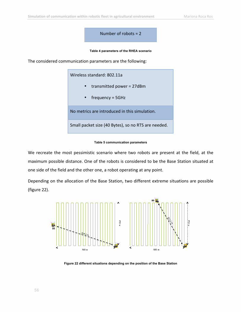
Simulation of communication within robotic fleet in agricultural environment Mariona Roca Ros
56
Number of robots = 2
Table 4 parameters of the RHEA scenario
The considered communication parameters are the following:
Wireless standard: 802.11a
• transmitted power = 27dBm
• frequency = 5GHz
No metrics are introduced in this simulation.
Small packet size (40 Bytes), so no RTS are needed.
Table 5 communication parameters
We recreate the most pessimistic scenario where two robots are present at the field, at the
maximum possible distance. One of the robots is considered to be the Base Station situated at
one side of the field and the other one, a robot operating at any point.
Depending on the allocation of the Base Station, two different extreme situations are possible
(figure 22).
Figure 22 different situations depending on the position of the Base Station
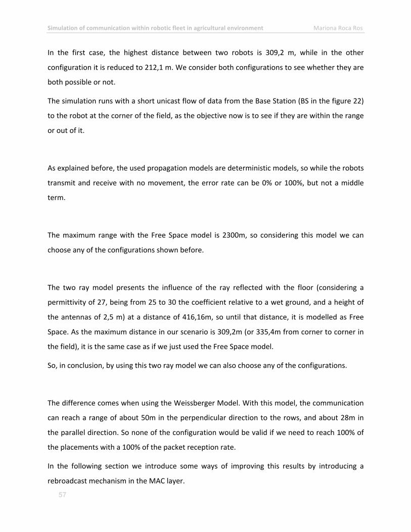
Simulation of communication within robotic fleet in agricultural environment Mariona Roca Ros
57
In the first case, the highest distance between two robots is 309,2 m, while in the other
configuration it is reduced to 212,1 m. We consider both configurations to see whether they are
both possible or not.
The simulation runs with a short unicast flow of data from the Base Station (BS in the figure 22)
to the robot at the corner of the field, as the objective now is to see if they are within the range
or out of it.
As explained before, the used propagation models are deterministic models, so while the robots
transmit and receive with no movement, the error rate can be 0% or 100%, but not a middle
term.
The maximum range with the Free Space model is 2300m, so considering this model we can
choose any of the configurations shown before.
The two ray model presents the influence of the ray reflected with the floor (considering a
permittivity of 27, being from 25 to 30 the coefficient relative to a wet ground, and a height of
the antennas of 2,5 m) at a distance of 416,16m, so until that distance, it is modelled as Free
Space. As the maximum distance in our scenario is 309,2m (or 335,4m from corner to corner in
the field), it is the same case as if we just used the Free Space model.
So, in conclusion, by using this two ray model we can also choose any of the configurations.
The difference comes when using the Weissberger Model. With this model, the communication
can reach a range of about 50m in the perpendicular direction to the rows, and about 28m in
the parallel direction. So none of the configuration would be valid if we need to reach 100% of
the placements with a 100% of the packet reception rate.
In the following section we introduce some ways of improving this results by introducing a
rebroadcast mechanism in the MAC layer.
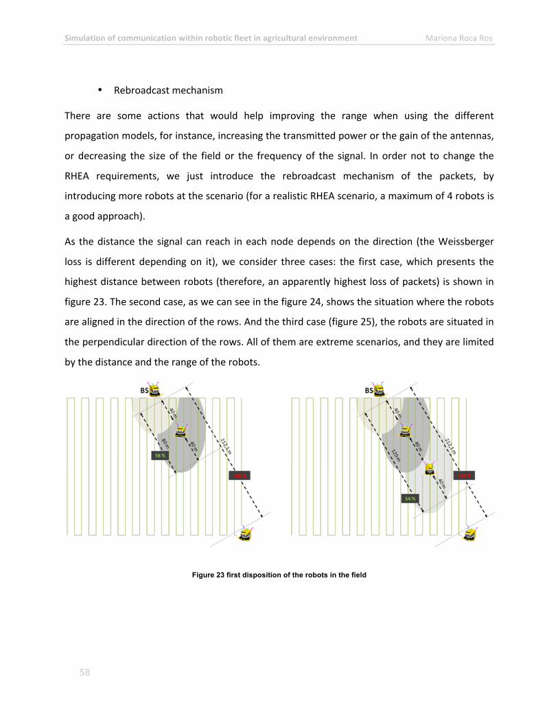
Simulation of communication within robotic fleet in agricultural environment Mariona Roca Ros
58
• Rebroadcast mechanism
There are some actions that would help improving the range when using the different
propagation models, for instance, increasing the transmitted power or the gain of the antennas,
or decreasing the size of the field or the frequency of the signal. In order not to change the
RHEA requirements, we just introduce the rebroadcast mechanism of the packets, by
introducing more robots at the scenario (for a realistic RHEA scenario, a maximum of 4 robots is
a good approach).
As the distance the signal can reach in each node depends on the direction (the Weissberger
loss is different depending on it), we consider three cases: the first case, which presents the
highest distance between robots (therefore, an apparently highest loss of packets) is shown in
figure 23. The second case, as we can see in the figure 24, shows the situation where the robots
are aligned in the direction of the rows. And the third case (figure 25), the robots are situated in
the perpendicular direction of the rows. All of them are extreme scenarios, and they are limited
by the distance and the range of the robots.
Figure 23 first disposition of the robots in the field
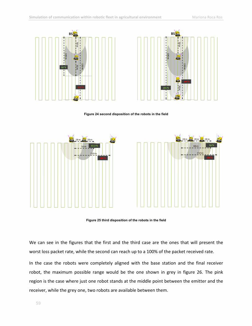
Simulation of communication within robotic fleet in agricultural environment Mariona Roca Ros
59
Figure 24 second disposition of the robots in the field
Figure 25 third disposition of the robots in the field
We can see in the figures that the first and the third case are the ones that will present the
worst loss packet rate, while the second can reach up to a 100% of the packet received rate.
In the case the robots were completely aligned with the base station and the final receiver
robot, the maximum possible range would be the one shown in grey in figure 26. The pink
region is the case where just one robot stands at the middle point between the emitter and the
receiver, while the grey one, two robots are available between them.
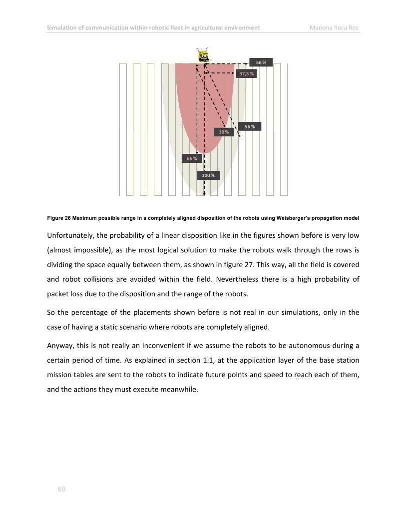
Simulation of communication within robotic fleet in agricultural environment Mariona Roca Ros
60
Figure 26 Maximum possible range in a completely aligned disposition of the robots using Weisberger’s propagation model
Unfortunately, the probability of a linear disposition like in the figures shown before is very low
(almost impossible), as the most logical solution to make the robots walk through the rows is
dividing the space equally between them, as shown in figure 27. This way, all the field is covered
and robot collisions are avoided within the field. Nevertheless there is a high probability of
packet loss due to the disposition and the range of the robots.
So the percentage of the placements shown before is not real in our simulations, only in the
case of having a static scenario where robots are completely aligned.
Anyway, this is not really an inconvenient if we assume the robots to be autonomous during a
certain period of time. As explained in section 1.1, at the application layer of the base station
mission tables are sent to the robots to indicate future points and speed to reach each of them,
and the actions they must execute meanwhile.
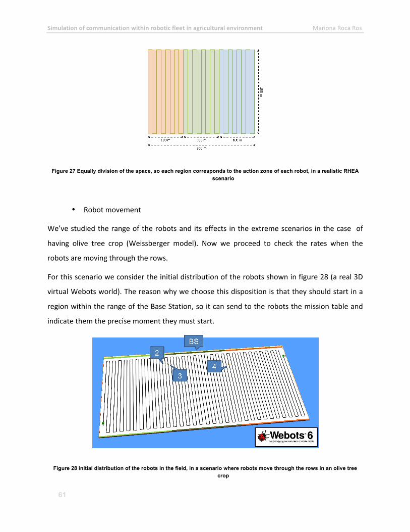
Simulation of communication within robotic fleet in agricultural environment Mariona Roca Ros
61
Figure 27 Equally division of the space, so each region corresponds to the action zone of each robot, in a realistic RHEA scenario
• Robot movement
We’ve studied the range of the robots and its effects in the extreme scenarios in the case of
having olive tree crop (Weissberger model). Now we proceed to check the rates when the
robots are moving through the rows.
For this scenario we consider the initial distribution of the robots shown in figure 28 (a real 3D
virtual Webots world). The reason why we choose this disposition is that they should start in a
region within the range of the Base Station, so it can send to the robots the mission table and
indicate them the precise moment they must start.
Figure 28 initial distribution of the robots in the field, in a scenario where robots move through the rows in an olive tree crop
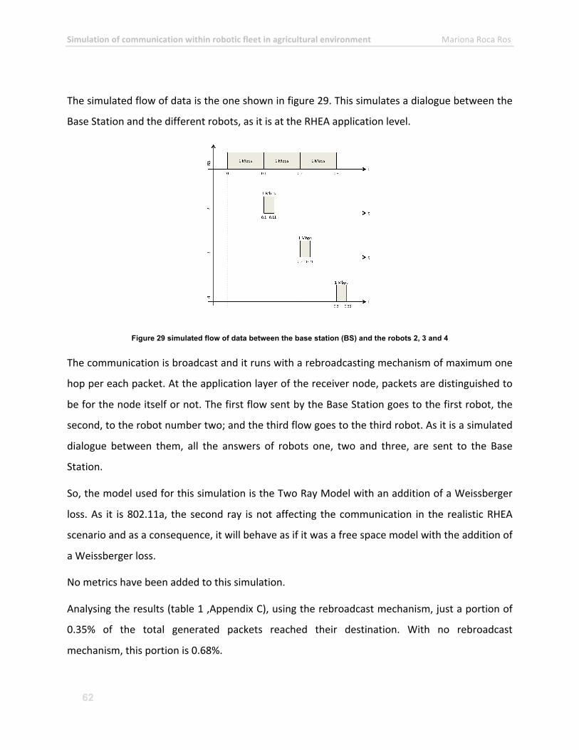
Simulation of communication within robotic fleet in agricultural environment Mariona Roca Ros
62
The simulated flow of data is the one shown in figure 29. This simulates a dialogue between the
Base Station and the different robots, as it is at the RHEA application level.
Figure 29 simulated flow of data between the base station (BS) and the robots 2, 3 and 4
The communication is broadcast and it runs with a rebroadcasting mechanism of maximum one
hop per each packet. At the application layer of the receiver node, packets are distinguished to
be for the node itself or not. The first flow sent by the Base Station goes to the first robot, the
second, to the robot number two; and the third flow goes to the third robot. As it is a simulated
dialogue between them, all the answers of robots one, two and three, are sent to the Base
Station.
So, the model used for this simulation is the Two Ray Model with an addition of a Weissberger
loss. As it is 802.11a, the second ray is not affecting the communication in the realistic RHEA
scenario and as a consequence, it will behave as if it was a free space model with the addition of
a Weissberger loss.
No metrics have been added to this simulation.
Analysing the results (table 1 ,Appendix C), using the rebroadcast mechanism, just a portion of
0.35% of the total generated packets reached their destination. With no rebroadcast
mechanism, this portion is 0.68%.
Simulation of communication within robotic fleet in agricultural environment Mariona Roca Ros
63
Now, using the same scenario, the communication within the robots is simulated in the
situation where the crop has not grown yet.
The only thing that changes respect the first simulation is the propagation model used. This
case, as we consider a flat and wet ground, where no other obstacles but the ground itself can
interfere the communication, a Two Ray model is used. In wet conditions, we consider a
permittivity of the floor of around 27 (25 -‐ 30). Considering 802.11a and the same height of the
antenna that has been used in previous simulations (2,5 meters), the reflected ray arrives at the
receiver node at a distance of around 416 meters. So the propagation model is equivalent to the
Free Space, in the RHEA scenario.
Looking at the results (table 2 ,Appendix C) without using a rebroadcast mechanism, we can see
an error rate of 89%. 100% of them caused by collisions between packets. None of them
because of lack of strength. This result is coherent, as the range in a Free Space propagation is
significatively bigger than the maximum distance between robots. So no propagation problems
are detected in this situation.
As there are no packets dropped because of the lack of strength, a high traffic is experienced in
the channel, and so, the probability of dropping a packet because of a collision is higher.
As shown in the table, when using a rebroadcasting mechanism a 6.6% of the packets are loss.
All of them due to collisions.
In order to check the influence of the Two Ray propagation model in the communication, we
run the same last simulation changing the wireless standard. Instead of IEEE 802.11a, we use
IEEE 802.11g. As this last standard works at a lower frequency (2,4GHz) and with lower
transmission power (0,1 mW), the second ray arrive at a shorter distance (around 216 meters,
instead of 416 meters in 802.11a). Therefore the communication will be slightly affected.
We expect a similar loss packet rate because even the loss due to the ray reflected at the
ground, the second ray starts affecting when the distance between them is around 216m. In the
chosen configuration, the maximum distance between the Base Station and the robot can be of
212m. So in this case it would not change the results. This would only be affected in case the
communication was between robots and not between robots and Base Station.
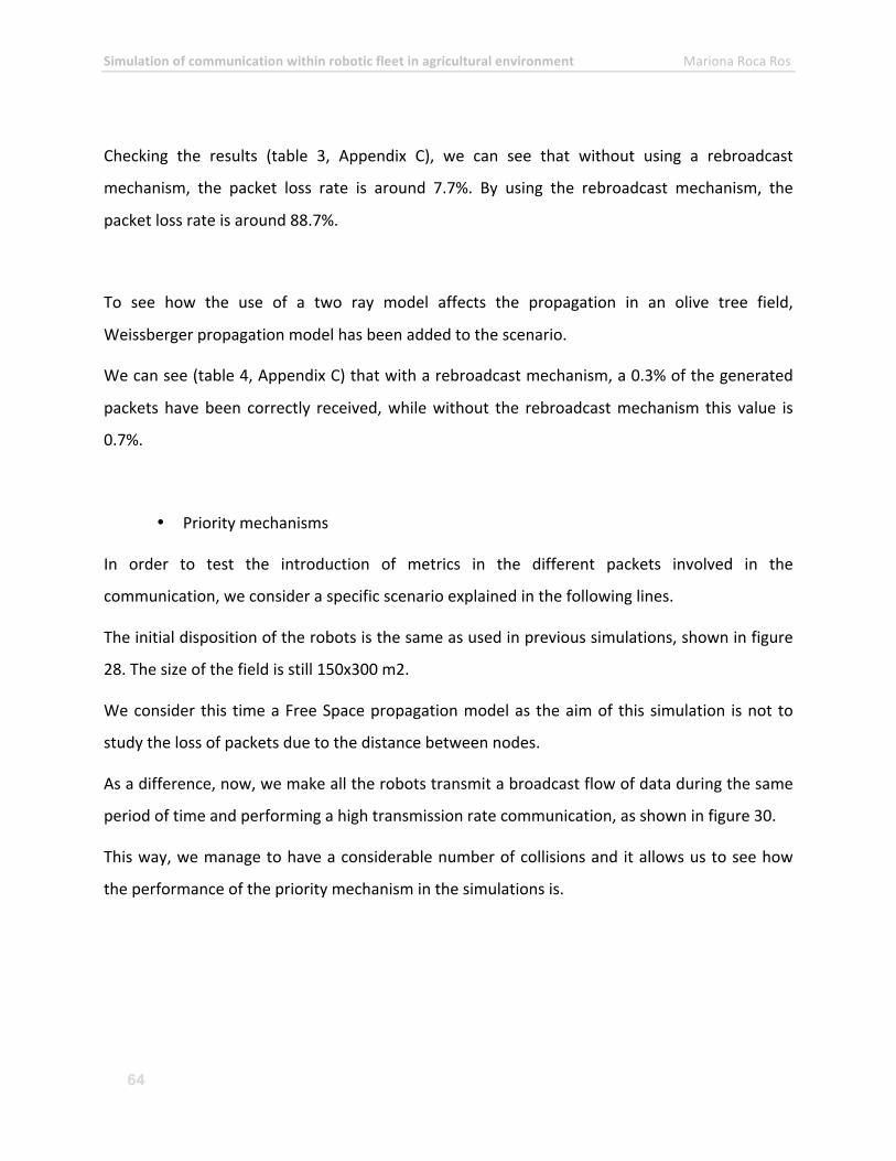
Simulation of communication within robotic fleet in agricultural environment Mariona Roca Ros
64
Checking the results (table 3, Appendix C), we can see that without using a rebroadcast
mechanism, the packet loss rate is around 7.7%. By using the rebroadcast mechanism, the
packet loss rate is around 88.7%.
To see how the use of a two ray model affects the propagation in an olive tree field,
Weissberger propagation model has been added to the scenario.
We can see (table 4, Appendix C) that with a rebroadcast mechanism, a 0.3% of the generated
packets have been correctly received, while without the rebroadcast mechanism this value is
0.7%.
• Priority mechanisms
In order to test the introduction of metrics in the different packets involved in the
communication, we consider a specific scenario explained in the following lines.
The initial disposition of the robots is the same as used in previous simulations, shown in figure
28. The size of the field is still 150x300 m2.
We consider this time a Free Space propagation model as the aim of this simulation is not to
study the loss of packets due to the distance between nodes.
As a difference, now, we make all the robots transmit a broadcast flow of data during the same
period of time and performing a high transmission rate communication, as shown in figure 30.
This way, we manage to have a considerable number of collisions and it allows us to see how
the performance of the priority mechanism in the simulations is.
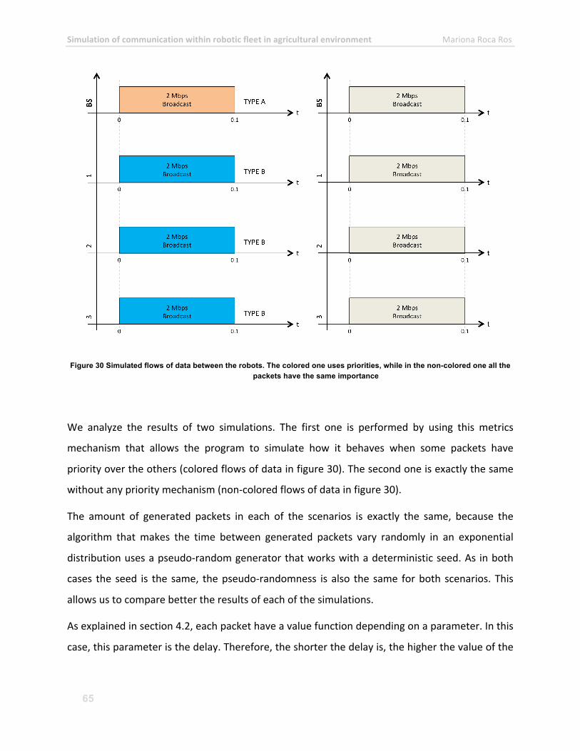
Simulation of communication within robotic fleet in agricultural environment Mariona Roca Ros
65
Figure 30 Simulated flows of data between the robots. The colored one uses priorities, while in the non-colored one all the packets have the same importance
We analyze the results of two simulations. The first one is performed by using this metrics
mechanism that allows the program to simulate how it behaves when some packets have
priority over the others (colored flows of data in figure 30). The second one is exactly the same
without any priority mechanism (non-‐colored flows of data in figure 30).
The amount of generated packets in each of the scenarios is exactly the same, because the
algorithm that makes the time between generated packets vary randomly in an exponential
distribution uses a pseudo-‐random generator that works with a deterministic seed. As in both
cases the seed is the same, the pseudo-‐randomness is also the same for both scenarios. This
allows us to compare better the results of each of the simulations.
As explained in section 4.2, each packet have a value function depending on a parameter. In this
case, this parameter is the delay. Therefore, the shorter the delay is, the higher the value of the
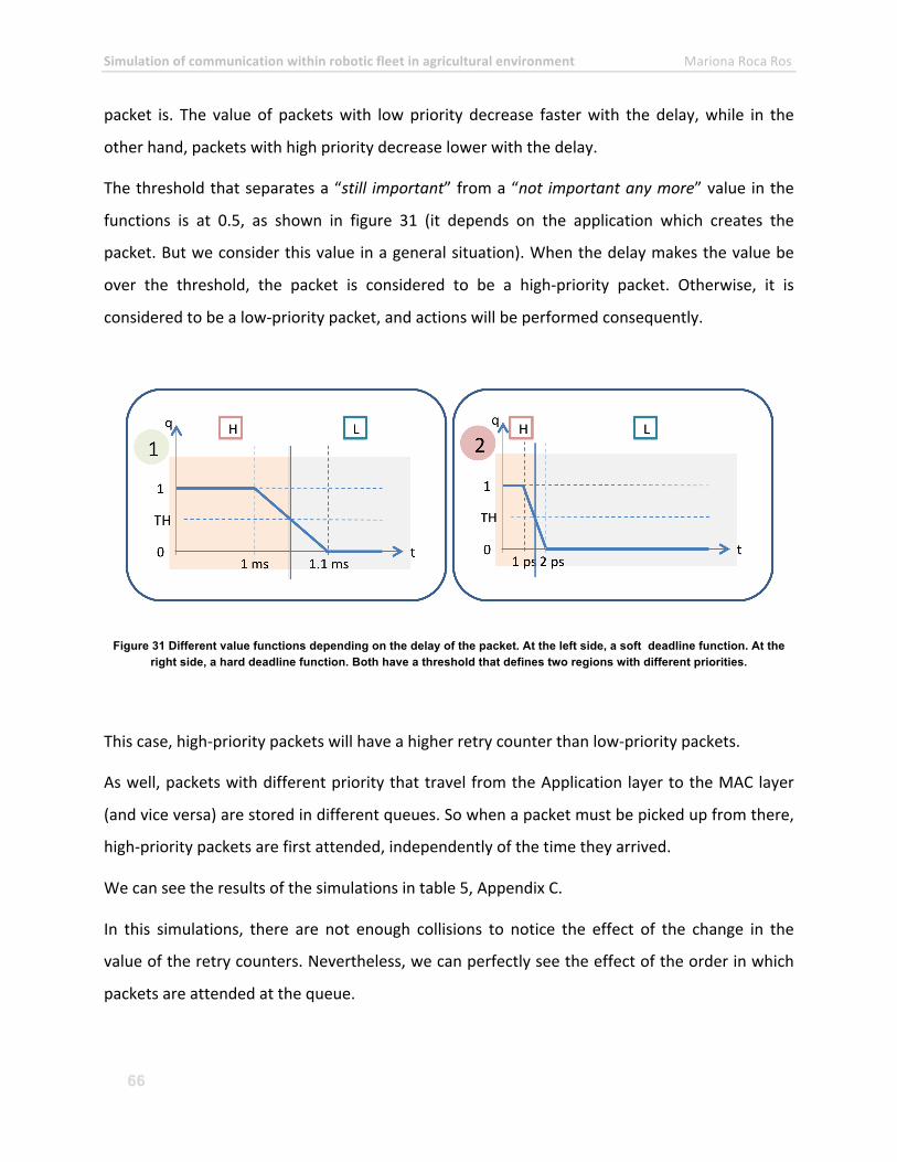
Simulation of communication within robotic fleet in agricultural environment Mariona Roca Ros
66
packet is. The value of packets with low priority decrease faster with the delay, while in the
other hand, packets with high priority decrease lower with the delay.
The threshold that separates a “still important” from a “not important any more” value in the
functions is at 0.5, as shown in figure 31 (it depends on the application which creates the
packet. But we consider this value in a general situation). When the delay makes the value be
over the threshold, the packet is considered to be a high-‐priority packet. Otherwise, it is
considered to be a low-‐priority packet, and actions will be performed consequently.
Figure 31 Different value functions depending on the delay of the packet. At the left side, a soft deadline function. At the right side, a hard deadline function. Both have a threshold that defines two regions with different priorities.
This case, high-‐priority packets will have a higher retry counter than low-‐priority packets.
As well, packets with different priority that travel from the Application layer to the MAC layer
(and vice versa) are stored in different queues. So when a packet must be picked up from there,
high-‐priority packets are first attended, independently of the time they arrived.
We can see the results of the simulations in table 5, Appendix C.
In this simulations, there are not enough collisions to notice the effect of the change in the
value of the retry counters. Nevertheless, we can perfectly see the effect of the order in which
packets are attended at the queue.
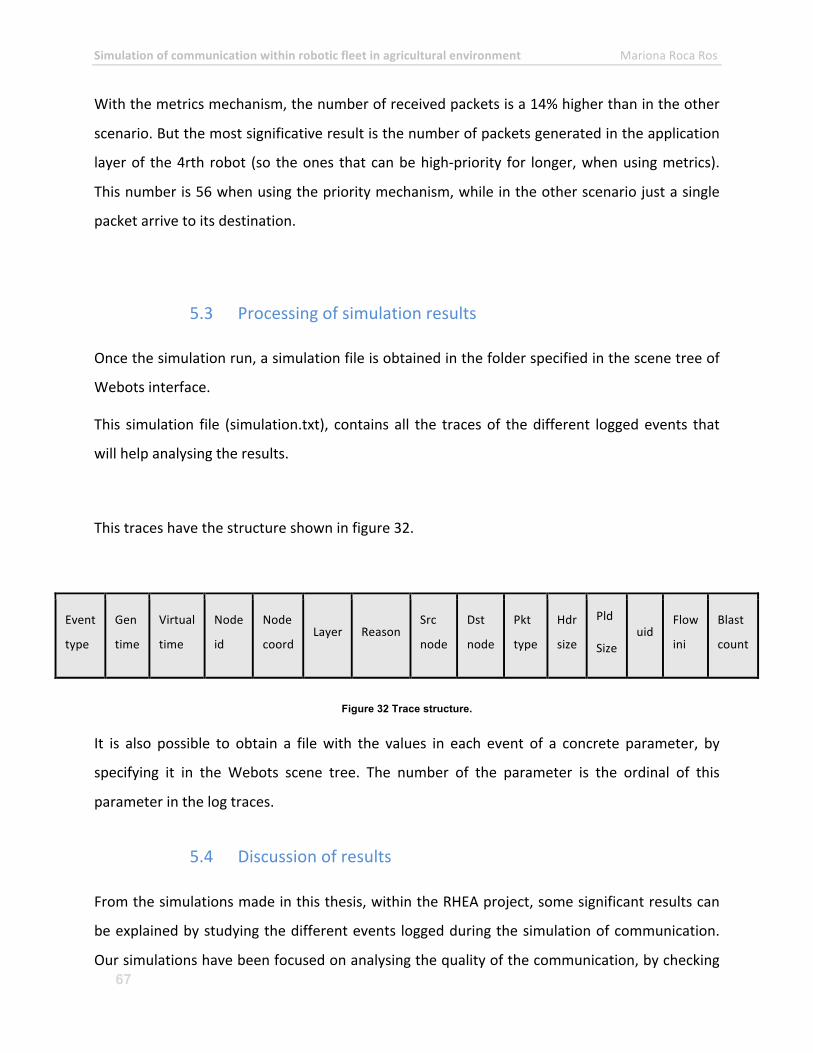
Simulation of communication within robotic fleet in agricultural environment Mariona Roca Ros
67
With the metrics mechanism, the number of received packets is a 14% higher than in the other
scenario. But the most significative result is the number of packets generated in the application
layer of the 4rth robot (so the ones that can be high-‐priority for longer, when using metrics).
This number is 56 when using the priority mechanism, while in the other scenario just a single
packet arrive to its destination.
5.3 Processing of simulation results
Once the simulation run, a simulation file is obtained in the folder specified in the scene tree of
Webots interface.
This simulation file (simulation.txt), contains all the traces of the different logged events that
will help analysing the results.
This traces have the structure shown in figure 32.
Event
type
Gen
time
Virtual
time
Node
id
Node
coord Layer Reason
Src
node
Dst
node
Pkt
type
Hdr
size
Pld
Size uid
Flow
ini
Blast
count
Figure 32 Trace structure.
It is also possible to obtain a file with the values in each event of a concrete parameter, by
specifying it in the Webots scene tree. The number of the parameter is the ordinal of this
parameter in the log traces.
5.4 Discussion of results
From the simulations made in this thesis, within the RHEA project, some significant results can
be explained by studying the different events logged during the simulation of communication.
Our simulations have been focused on analysing the quality of the communication, by checking
Simulation of communication within robotic fleet in agricultural environment Mariona Roca Ros
68
the loss of packets and the correct packet reception in each link. For that we specially studied
the range when having different propagation models and the behaviour of packet reception
when having priority packets.
No range problems are found when the crops have not grown yet. Even in the highest possible
distances between robots, packets can be received with enough strength to be processed by the
application layer of the receiver.
Things change when having an Olive Tree crop. By using the Weissberger model, we can
appreciate that a higher loss of data is produced when the robots are moving through the rows.
The range in this crop describes an ellipse around the emitter, and reaches around 56m in the
perpendicular direction to the rows (84m by adding a rebroadcast mechanism), and 99m in the
direction of the rows (150m by adding a rebroadcast mechanism). It makes us think about some
concepts like, for example, the autonomy of the robots, or the density of the robot fleet (dense
or sparse).
When recreating a dialogue between the robots, collisions must be also taken into account.
Specially in a scenario with wet floor (with no grown crop), where there are no obstacles in the
communication, and as all packets can arrive to its destination, the traffic is higher than in any
other situation. We can see in the results of the simulations that a 89% of the packets are
dropped because of collisions in this scenario when using rebroadcast mechanism, but just a
6.6% if this rebroadcast mechanism is not used. Therefore, in applications generating a high
traffic through the channel, collisions must be specially taken into account, as the loss packet
rate is directly related to the packet generation rate.
As said before, if there are obstacles between the robots, then the packet collision rate gets
lower because of the decrease of the traffic in the links. In the other hand, it increases the
number of loss packets due to the short range of the emitter.
In order to give priority to some packets, some simulations run with defined metrics in each of
the packets. In our case, we gave a higher value function to the packets generated in the base
station, and a lower value function to all the others. Packets with higher value function keep the
Simulation of communication within robotic fleet in agricultural environment Mariona Roca Ros
69
high priority flag longer than the others. When at any point in the communication stack a packet
is detected to be a high priority packet, some actions can be performed, like for example, in our
scenario, increasing the retry counter to make the probability of correct reception at the
receiver higher.
These lasts simulations help us see that when different priority-‐packets are received, the high
priority ones are first processed even if they arrived later at the node.
The performed simulations also help us to determine the time a simulation last. It is not an
exact value as it depends on the number and frequency of the events, and the computation
capacity needed to process them. For example, broadcast communication simulations are
definitely faster than unicast ones, as no control packets are generated.
In the simulations performed in this thesis, the virtual time of the simulator changed between
70% of the real time and 10% of it. This virtual time, though, is not the time of our simulations,
as in our algorithms the scheduler has been scaled in time. All our simulations have been
performed with a scale factor of 6500. So at the end, there is a factor of 2000 between the real
time and the simulation scaled time.
For example, to simulate 0.5 seconds of a broadcast communication with a packet generation
speed of 2Mbps in each of the four robots involved in the simulation, around 17 minutes are
needed.
5.5 Possible extensions
Through the simulations some aspects in the communication within or outside the RHEA
scenarios can be more accurately studied in the future.
In relation to the different metrics added to the packets, in this thesis it has just been focused
the management of priorities. But not all the possible actions that can be performed when a
packet is detected to have a certain priority level. Changes in the contention window of the
backoff mechanism; putting extreme values in the retry counters when the reception of a
Simulation of communication within robotic fleet in agricultural environment Mariona Roca Ros
70
packet fails; or even more than two priority levels can be added in the simulations just by
adding more queues at the buffer between the Application and the MAC layer. These are some
examples of the possible extensions performed in this way.
Regarding the propagation models, in this thesis we dealed with the extreme situations of
having no grown crops (flat wet ground) or having the most dense possible crops in RHEA (the
olive tree). Nevertheless, more models can be added in order to simulate all the possible crops
in RHEA.
Simulation of communication within robotic fleet in agricultural environment Mariona Roca Ros
71
6. Conclusion
6.1 Contribution
Since Webots is a commonly used software package to model, program and simulate mobile
robots in commercial and in research environments, the main contribution of this thesis is to
develop new functionalities in order to be able to make more reliable simulations of the
communication between robots.
Until now, no communication standards were available in this simulator, so simulation of
communication was just possible at the physical layer.
Basing on the algorithm already developed for NS2 architecture, a simple and modular scheme
has been created for the Webots architecture. This will allow an easy implementation of other
standards just by following the structure of the scheduler and the layers already developed in
this thesis.
IEEE 802.11 standard has been implemented. As well, this implementation has been checked
through some realistic agricultural scenarios (within the EU RHEA project). This way, and by
adapting the propagation model and the general performance to this scenarios, the wireless
communication between robots and the base station has been run and checked.
Therefore, through the analysis of the simulation results, the quality of communication and its
range has been obtained, and made us think about some concepts such as the autonomy of the
robots, or the density of the fleet. The discussion of this concepts and its application, makes the
communication within the fleet easier, and consequently, the objectives of the RHEA project to
be easily achieved.
Nevertheless, the discussion of this concepts in RHEA must be done in future work, as well as
the implementation of other communication standards (such as ZigBee).
Simulation of communication within robotic fleet in agricultural environment Mariona Roca Ros
72
6.2 Outlook
After analyzing the current situation of the networked robots, the problem of simulating the
communication in an already existing mobile robot simulator tool has been described. The aim
of this thesis is to implement new functionalities for this simulator so mobile robot simulations
can include the simulation of the communication by using WLAN.
With this purpose, the requirements of the communication within the RHEA robotic fleet have
been defined in terms of maximum data speed and the minimum packet loss rate. Basing on this
requirements, the implementation of WLAN IEEE 802.11 has been developed in a modular and
structured way, so new standards can be easily implemented in the future by following the
same structure.
In order to implement the standard IEEE 802.11, the algorithm used in NS2 (an event-‐based
network simulator) has been adapted to the architecture of Webots (a time-‐based network
simulator). It required the creation of a scheduler and a layered structure. The scheduler is not
only needed to create events (packet passing from one layer to the other one), but also to
implement the timeouts of the timers defined in the different modules of the MAC and the
Physical layer (modelled as state-‐event machines).
The way time-‐based simulator is ruled by the scheduler, is to create a special event that makes
the simulation move forward one step of time. Therefore, when this event is attended, all the
devices in the world defined in the simulator, compute one step of time.
The adaptation of the algorithm required the adaptation of the Emitter node in the Webots
interface, so the user can specify the parameters through the simulator and so there is no need
to deal with the code.
As time in Webots evolves from a step of time to an other step of time, the time definition was
not precise enough for timers to work normally. Therefore, a scaling of the timeline in the
scheduler was required, and it implied a slow down of the simulator.
The adapted algorithm have been complemented with some propagation models that suited
with some RHEA realistic scenarios (such as Weissberger model, which models a vegetation
environment). A rebroadcast mechanism has also been implemented and also metrics have
Simulation of communication within robotic fleet in agricultural environment Mariona Roca Ros
73
been introduced to give the packets a value according to their importance and to their delay in
the communication.
Once the algorithm is completely adapted, the evaluation of the implementation has been
tested by recreating simple scenarios and checking the behaviour of the communication.
After the implementation has been tested and verified, we proceeded to recreate some realistic
RHEA scenarios in order to check if the configuration of the scenarios is appropriate when using
this standard.
The conclusions we can take from the simulations are that when the crop is not grown, and
considering a wet floor, a packet loss rate can reach the 7% of the total sent packets if we don’t
introduce a rebroadcast mechanism in the communication. If we do, this packet loss rate can
reach a value around 89%. This difference appears because the increment of the traffic, which
makes the collision probability sharply increase.
Therefore, it is important to pay special attention to the compromise between increasing the
range of a node (by adding a rebroadcast mechanism), and keeping a low packet loss rate.
In the other hand, problems arrive when having an already grown Olive Tree crop. In this
situation, and using the rebroadcast mechanism, the range can cover up to a 56% of the space
in the perpendicular direction to the rows, and a 100% in the parallel direction. Even though,
this result is a limit, but the probability of having this results is very low, as having the robots
completely aligned is almost impossible due to the field distribution between the robots. At this
point, the use of other standards such as ZigBee is required, or otherwise, some properties in
the scenario such as the autonomy of the robots, or the density of the fleet must be considered.
In this sense, it must be taken into account that having a dense fleet could seemly imply less
needed autonomy in the robots, but could lead to a situation in which the robots in the sides
could not reach the signal of the base station. Otherwise, having a sparse fleet would lead us to
have a long time of autonomy in the robots, even though all of them could reach the signal of
the base station at some time.
Simulation of communication within robotic fleet in agricultural environment Mariona Roca Ros
74
The situation of having metrics in the packets has also been checked. In the simulations, we
could appreciate that the high priority packets were first processed even if they arrived later at
the node.
The time a simulation last has also been discussed, and even it depends on the frequency of
events and in the needed computation capacity to process them, to make the simulations
performed in this thesis, a factor of 2000 between the real time and the simulation scaled time
was present. So it makes the simulation slow down and must be taken into account when
setting out a new scenario to simulate.
The new aspects to be considered in the future work are the implementation of new standards,
such as ZigBee, or the implementation of more propagation models.
In RHEA, the implementation of new functionalities in the Application Layer according to its
scenarios will be necessary to implement the real behaviour of the robots in the project.
Some new functionalities in the nodes can be provided, such as the possibility of adding more
interfaces to the nodes.
As well, the optimization of the time a simulation last would be a good improve when adding
communication features to the simulations.
Simulation of communication within robotic fleet in agricultural environment Mariona Roca Ros
75
7. References
[1] Lynne E. Parker , “Chapter 40, Multiple Mobile Robot Systems”, Mobile and Distributed
Robotics.
[2] John Billingsley, Arto Visala, Mark Dunn, “Chapter 46, Robotics in Agriculture and Forestry”,
Mobile and Distributed Robotics.
[3] Dezhen Song, Ken Goldberg, Nak Young Chong , “Chapter 32, Networked Telerobots”,
Mobile and Distributed Robotics.
[4] Vijay Kumar, Daniela Rus, Gaurav S. Sukhatme, “Chapter 41, Networked Robots”, Mobile
and Distributed Robotics.
[5] P.Gonzalez-‐de-‐Santos and A.Ribeiro, “Description of the High-‐level decision making system
(D.4.1)”, EU. RHEA project.
[6] Wikipedia, “Resilience”.
[7] Wikipedia, “Synchronization”.
[8] Wikipedia, “Synchronization in Telecommunications”.
[9] Wikipedia, “Metrics (networking)”.
[10] Wikipedia, “Modelo OSI”.
[11] Wikipedia, “IEEE 802.11”.
[12] Qi Chen, Felix Schmidt-‐Eisenlohr, Daniel Jiang, Marc Torrent-‐Moreno, Luca Delgrossi,
Hannes Hartenstein, “Overhaul of IEEE 802.11 Modelling and Simulation in NS-‐2”.
[13] Broadcom, “The new mainstream Wireless LAN standard”.
[14] M.Roca, S.Tomic, “Simulation of Communication within the RHEA Robotic Fleet”.
[15] Webots "User Guide", http://www.cyberbotics.com/
[16] Webots "Reference manual", http://www.cyberbotics.com/
[17] Wikipedia, “ZigBee”
[18] "Network Simulator ns-‐2", http://www.isi.edu/nsnam/ns
Simulation of communication within robotic fleet in agricultural environment Mariona Roca Ros
76
[19] Kevin Fall, Kannan Varadhan, “The ns Manual (formerly ns Notes and Documentation)”,
The VINT Project.
[20] Dr Grahan Brooker , “Sensors and Signals”, University of Sydney, 2006.
[21] Christoph Sommer, Falko Dressler, “Using the Right Two-‐Ray Model? A measurement-‐
based Evaluation of PHY Models in VANETs”, Institute of Computer Science, University of
Innsbruck, Austria.
[22] Verdone, Roberto; Dardari, Davide; Mazzini, Gianluca; Conti, Andrea, “Wireless Sensor and
Actuator Networks-‐Technologies, Analysis and Design”. ©2008 Elsevier.
[23] John Thelen, Daan Goense, Koen Langendoen, “Radio Wave Propagation in Potato Fields”.
[24] Pedro Mestre, José Ribeiro, Carlos Serodio, Joao Monteiro, “Propagation of IEEE802.15.4 in
Vegetation”.
[25] L.M.Kamarudin, R.B.Ahmad, B.L.Ong, A.Zakaria, D.Ndzi, “Modelling and Simulation of near-‐
earth Wireless Sensor Networks for Agriculture based Application using OMNeT++”.
[26] E.G.Ström, E.Uhlemann, C.F.Mecklenbräuker, “Performance metrics for mobile-‐to-‐mobile
communications”.
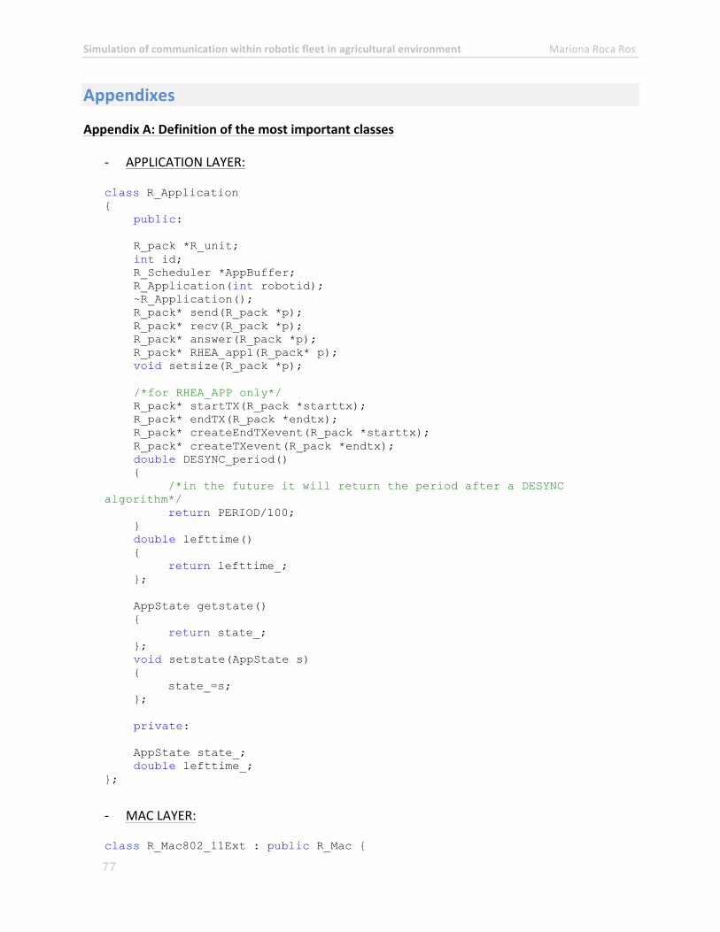
Simulation of communication within robotic fleet in agricultural environment Mariona Roca Ros
77
Appendixes
Appendix A: Definition of the most important classes
-‐ APPLICATION LAYER:
class R_Application { public: R_pack *R_unit; int id; R_Scheduler *AppBuffer; R_Application(int robotid); ~R_Application(); R_pack* send(R_pack *p); R_pack* recv(R_pack *p); R_pack* answer(R_pack *p); R_pack* RHEA_app1(R_pack* p); void setsize(R_pack *p); /*for RHEA_APP only*/ R_pack* startTX(R_pack *starttx); R_pack* endTX(R_pack *endtx); R_pack* createEndTXevent(R_pack *starttx); R_pack* createTXevent(R_pack *endtx); double DESYNC_period() { /*in the future it will return the period after a DESYNC algorithm*/ return PERIOD/100; } double lefttime() { return lefttime_; }; AppState getstate() { return state_; }; void setstate(AppState s) { state_=s; }; private: AppState state_; double lefttime_; };
-‐ MAC LAYER:
class R_Mac802_11Ext : public R_Mac {
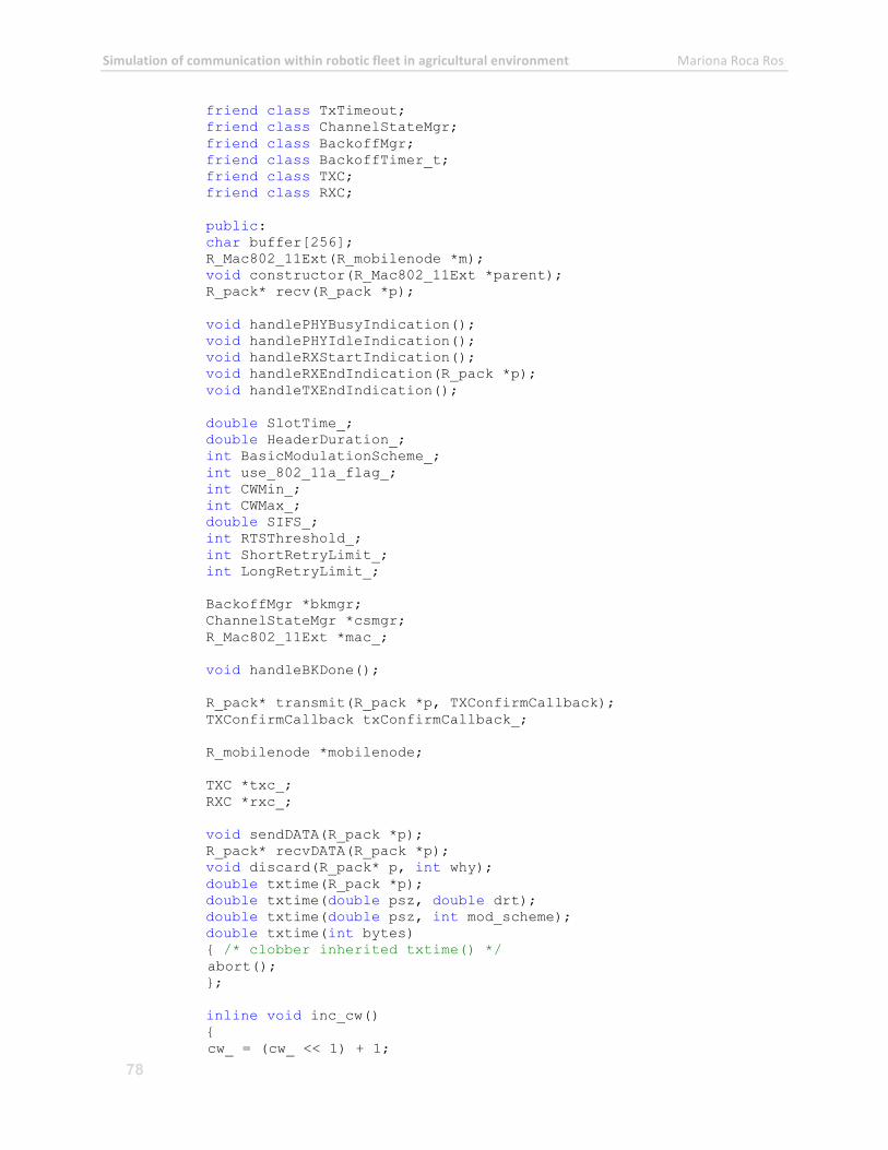
Simulation of communication within robotic fleet in agricultural environment Mariona Roca Ros
78
friend class TxTimeout; friend class ChannelStateMgr; friend class BackoffMgr; friend class BackoffTimer_t; friend class TXC; friend class RXC; public: char buffer[256]; R_Mac802_11Ext(R_mobilenode *m); void constructor(R_Mac802_11Ext *parent); R_pack* recv(R_pack *p); void handlePHYBusyIndication(); void handlePHYIdleIndication(); void handleRXStartIndication(); void handleRXEndIndication(R_pack *p); void handleTXEndIndication(); double SlotTime_; double HeaderDuration_; int BasicModulationScheme_; int use_802_11a_flag_; int CWMin_; int CWMax_; double SIFS_; int RTSThreshold_; int ShortRetryLimit_; int LongRetryLimit_; BackoffMgr *bkmgr; ChannelStateMgr *csmgr; R_Mac802_11Ext *mac_; void handleBKDone(); R_pack* transmit(R_pack *p, TXConfirmCallback); TXConfirmCallback txConfirmCallback_; R_mobilenode *mobilenode; TXC *txc_; RXC *rxc_; void sendDATA(R_pack *p); R_pack* recvDATA(R_pack *p); void discard(R_pack* p, int why);
double txtime(R_pack *p); double txtime(double psz, double drt); double txtime(double psz, int mod_scheme); double txtime(int bytes) { /* clobber inherited txtime() */ abort(); }; inline void inc_cw() { cw_ = (cw_ << 1) + 1;
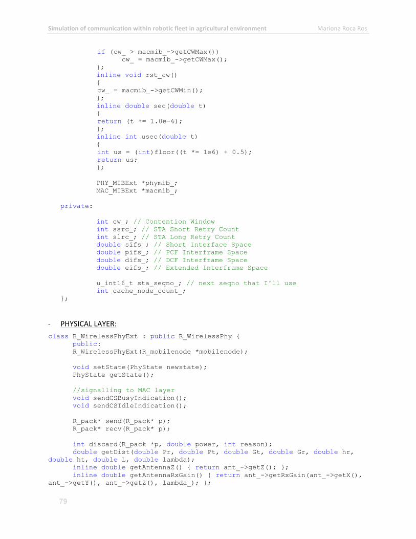
Simulation of communication within robotic fleet in agricultural environment Mariona Roca Ros
79
if (cw_ > macmib_->getCWMax()) cw_ = macmib_->getCWMax(); }; inline void rst_cw() { cw_ = macmib_->getCWMin(); }; inline double sec(double t) { return (t *= 1.0e-6); }; inline int usec(double t) { int us = (int)floor((t *= 1e6) + 0.5); return us; }; PHY_MIBExt *phymib_; MAC_MIBExt *macmib_; private: int cw_; // Contention Window int ssrc_; // STA Short Retry Count int slrc_; // STA Long Retry Count double sifs_; // Short Interface Space double pifs_; // PCF Interframe Space double difs_; // DCF Interframe Space double eifs_; // Extended Interframe Space u_int16_t sta_seqno_; // next seqno that I'll use int cache_node_count_; };
-‐ PHYSICAL LAYER: class R_WirelessPhyExt : public R_WirelessPhy {
public: R_WirelessPhyExt(R_mobilenode *mobilenode); void setState(PhyState newstate); PhyState getState(); //signalling to MAC layer void sendCSBusyIndication(); void sendCSIdleIndication(); R_pack* send(R_pack* p); R_pack* recv(R_pack* p); int discard(R_pack *p, double power, int reason);
double getDist(double Pr, double Pt, double Gt, double Gr, double hr, double ht, double L, double lambda);
inline double getAntennaZ() { return ant_->getZ(); }; inline double getAntennaRxGain() { return ant_->getRxGain(ant_->getX(),
ant_->getY(), ant_->getZ(), lambda_); };

Simulation of communication within robotic fleet in agricultural environment Mariona Roca Ros
80
inline double getAntennaTxGain() { return ant_->getTxGain(ant_->getX(), ant_->getY(), ant_->getZ(), lambda_); };
inline double getPowerMonitorThresh() { return PowerMonitorThresh_; }; int sendchannel(R_pack *p);
R_pack *control; R_mobilenode *m; double lambda_; // wavelength (m) double L_; // system loss factor double CSThresh_ext; // carrier sense threshold (W) fixed by chipset double CPThresh_ext; // capture threshold double RXThresh_ext; // capture threshold double Pt_; // transmitted signal power (W) double freq_; // frequency double HeaderDuration_; // preamble+SIGNAL int BasicModulationScheme_; int PreambleCaptureSwitch_; //PreambleCaptureSwitch int DataCaptureSwitch_; //DataCaptureSwitch double SINR_PreambleCapture_; double SINR_DataCapture_; double trace_dist_; double noise_floor_; double PowerMonitorThresh_; //R_FreeSpace *propagation_; R_TwoRayModel *propagation_; //R_Weissberger *propagation_; R_OmniAntenna *ant_; R_PowerMonitor *powerMonitor; PhyState state; PhyState oldstate; R_pack *pkt_RX; R_pack *pkt_TX; double SINR_Th_RX; //SINR threshold for decode data according to the modulation scheme double power_RX; R_pack *rX_Timer; R_pack *preRX_Timer; R_pack *tX_Timer; double SINR_Th(int R_modulationScheme); friend class R_PowerMonitor;
};
-‐ PRERECEIVE LAYER: class R_prerec { public: R_prerec();
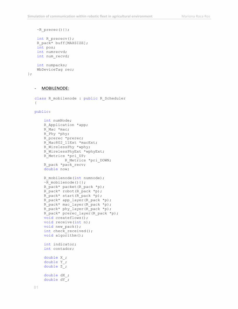
Simulation of communication within robotic fleet in agricultural environment Mariona Roca Ros
81
~R_prerec(){}; int R_prerecv(); R_pack* buff[MAXSIZE]; int pos; int numrecvd; int num_recvd; int numpacks; WbDeviceTag rec; };
-‐ MOBILENODE:
class R_mobilenode : public R_Scheduler { public: int numNode; R_Application *app; R_Mac *mac; R_Phy *phy; R_prerec *prerec; R_Mac802_11Ext *macExt; R_WirelessPhy *wphy; R_WirelessPhyExt *wphyExt; R_Metrics *pri_UP;
R_Metrics *pri_DOWN; R_pack *pack_recv; double now; R_mobilenode(int numnode); ~R_mobilenode(){}; R_pack* packet(R_pack *p); R_pack* robot(R_pack *p); R_pack* start(R_pack *p); R_pack* app_layer(R_pack *p); R_pack* mac_layer(R_pack *p); R_pack* phy_layer(R_pack *p); R_pack* prerec_layer(R_pack *p); void createflows(); void receive(int n); void new_pack(); int check_received(); void algorithm(); int indicator; int contador; double X_; double Y_; double Z_; double dX_; double dY_;
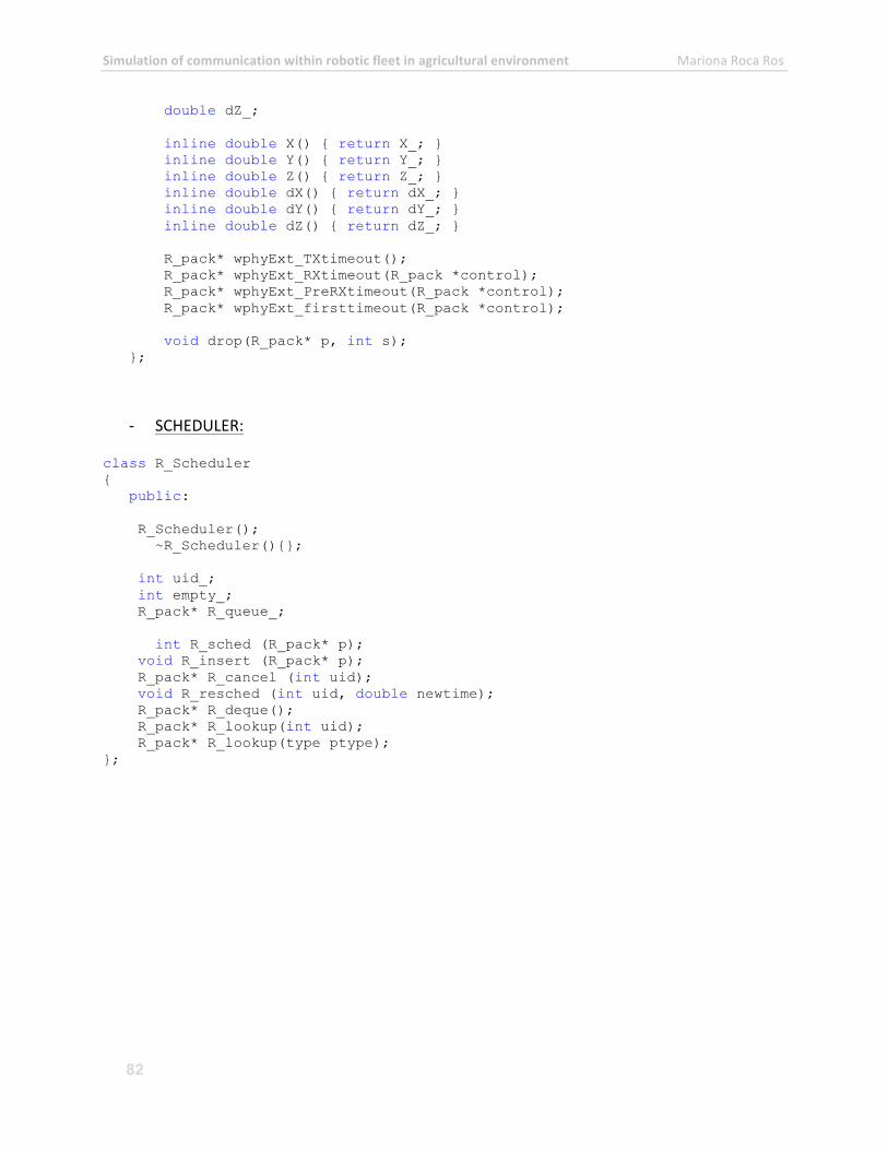
Simulation of communication within robotic fleet in agricultural environment Mariona Roca Ros
82
double dZ_; inline double X() { return X_; } inline double Y() { return Y_; } inline double Z() { return Z_; } inline double dX() { return dX_; } inline double dY() { return dY_; } inline double dZ() { return dZ_; } R_pack* wphyExt_TXtimeout(); R_pack* wphyExt_RXtimeout(R_pack *control); R_pack* wphyExt_PreRXtimeout(R_pack *control); R_pack* wphyExt_firsttimeout(R_pack *control); void drop(R_pack* p, int s); };
-‐ SCHEDULER:
class R_Scheduler { public: R_Scheduler(); ~R_Scheduler(){}; int uid_; int empty_; R_pack* R_queue_; int R_sched (R_pack* p); void R_insert (R_pack* p); R_pack* R_cancel (int uid); void R_resched (int uid, double newtime); R_pack* R_deque(); R_pack* R_lookup(int uid); R_pack* R_lookup(type ptype); };
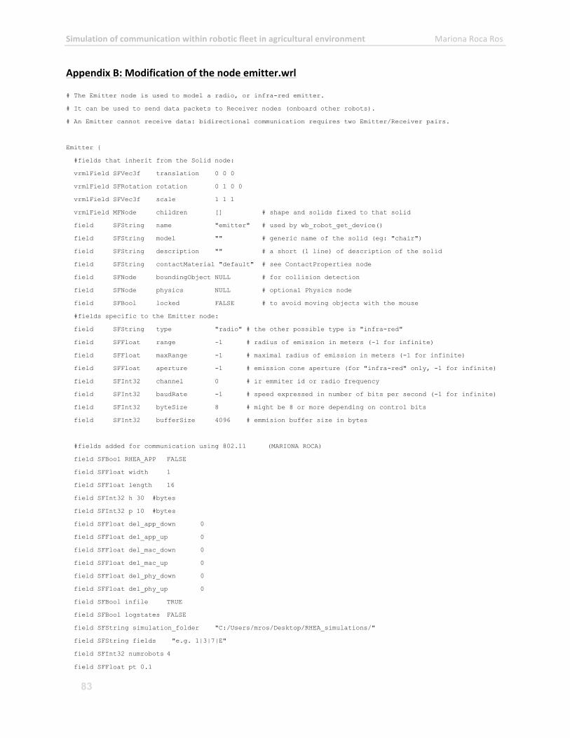
Simulation of communication within robotic fleet in agricultural environment Mariona Roca Ros
83
Appendix B: Modification of the node emitter.wrl
# The Emitter node is used to model a radio, or infra-red emitter.
# It can be used to send data packets to Receiver nodes (onboard other robots).
# An Emitter cannot receive data: bidirectional communication requires two Emitter/Receiver pairs.
Emitter {
#fields that inherit from the Solid node:
vrmlField SFVec3f translation 0 0 0
vrmlField SFRotation rotation 0 1 0 0
vrmlField SFVec3f scale 1 1 1
vrmlField MFNode children [] # shape and solids fixed to that solid
field SFString name "emitter" # used by wb_robot_get_device()
field SFString model "" # generic name of the solid (eg: "chair")
field SFString description "" # a short (1 line) of description of the solid
field SFString contactMaterial "default" # see ContactProperties node
field SFNode boundingObject NULL # for collision detection
field SFNode physics NULL # optional Physics node
field SFBool locked FALSE # to avoid moving objects with the mouse
#fields specific to the Emitter node:
field SFString type "radio" # the other possible type is "infra-red"
field SFFloat range -1 # radius of emission in meters (-1 for infinite)
field SFFloat maxRange -1 # maximal radius of emission in meters (-1 for infinite)
field SFFloat aperture -1 # emission cone aperture (for "infra-red" only, -1 for infinite)
field SFInt32 channel 0 # ir emmiter id or radio frequency
field SFInt32 baudRate -1 # speed expressed in number of bits per second (-1 for infinite)
field SFInt32 byteSize 8 # might be 8 or more depending on control bits
field SFInt32 bufferSize 4096 # emmision buffer size in bytes
#fields added for communication using 802.11 (MARIONA ROCA)
field SFBool RHEA_APP FALSE
field SFFloat width 1
field SFFloat length 16
field SFInt32 h 30 #bytes
field SFInt32 p 10 #bytes
field SFFloat del_app_down 0
field SFFloat del_app_up 0
field SFFloat del_mac_down 0
field SFFloat del_mac_up 0
field SFFloat del_phy_down 0
field SFFloat del_phy_up 0
field SFBool infile TRUE
field SFBool logstates FALSE
field SFString simulation_folder "C:/Users/mros/Desktop/RHEA_simulations/"
field SFString fields "e.g. 1|3|7|E"
field SFInt32 numrobots 4
field SFFloat pt 0.1
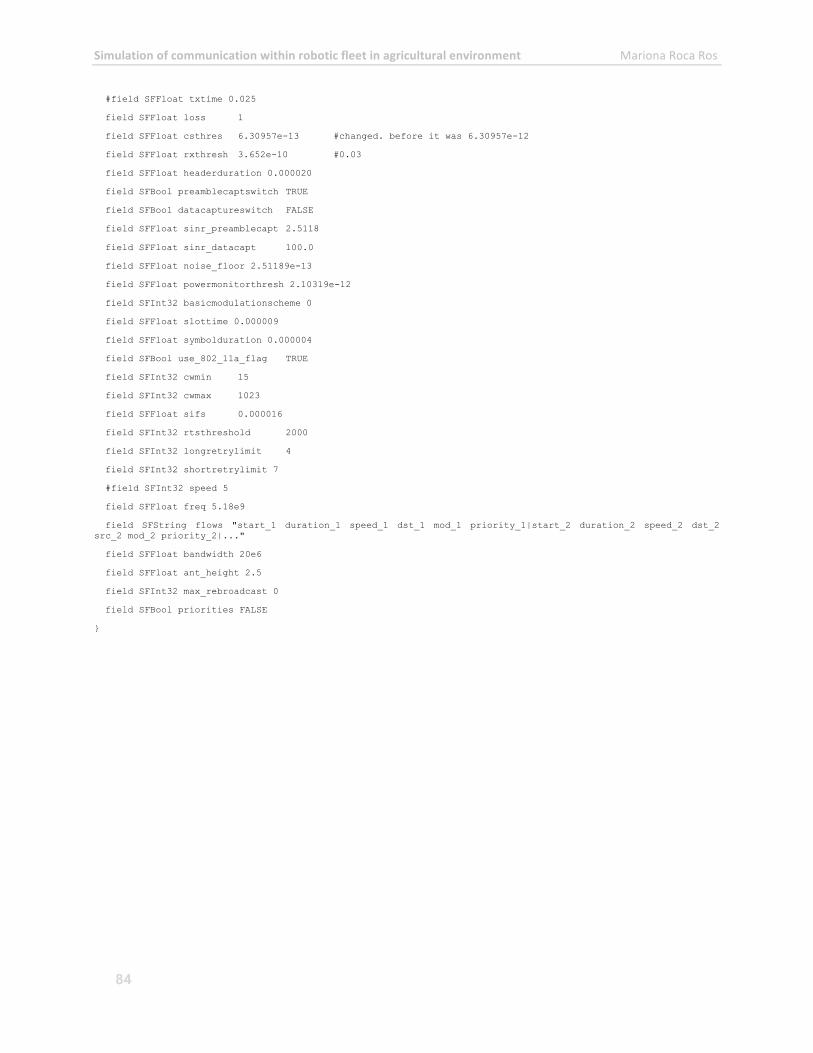
Simulation of communication within robotic fleet in agricultural environment Mariona Roca Ros
84
#field SFFloat txtime 0.025
field SFFloat loss 1
field SFFloat csthres 6.30957e-13 #changed. before it was 6.30957e-12
field SFFloat rxthresh 3.652e-10 #0.03
field SFFloat headerduration 0.000020
field SFBool preamblecaptswitch TRUE
field SFBool datacaptureswitch FALSE
field SFFloat sinr_preamblecapt 2.5118
field SFFloat sinr_datacapt 100.0
field SFFloat noise_floor 2.51189e-13
field SFFloat powermonitorthresh 2.10319e-12
field SFInt32 basicmodulationscheme 0
field SFFloat slottime 0.000009
field SFFloat symbolduration 0.000004
field SFBool use_802_11a_flag TRUE
field SFInt32 cwmin 15
field SFInt32 cwmax 1023
field SFFloat sifs 0.000016
field SFInt32 rtsthreshold 2000
field SFInt32 longretrylimit 4
field SFInt32 shortretrylimit 7
#field SFInt32 speed 5
field SFFloat freq 5.18e9
field SFString flows "start_1 duration_1 speed_1 dst_1 mod_1 priority_1|start_2 duration_2 speed_2 dst_2 src_2 mod_2 priority_2|..."
field SFFloat bandwidth 20e6
field SFFloat ant_height 2.5
field SFInt32 max_rebroadcast 0
field SFBool priorities FALSE
}
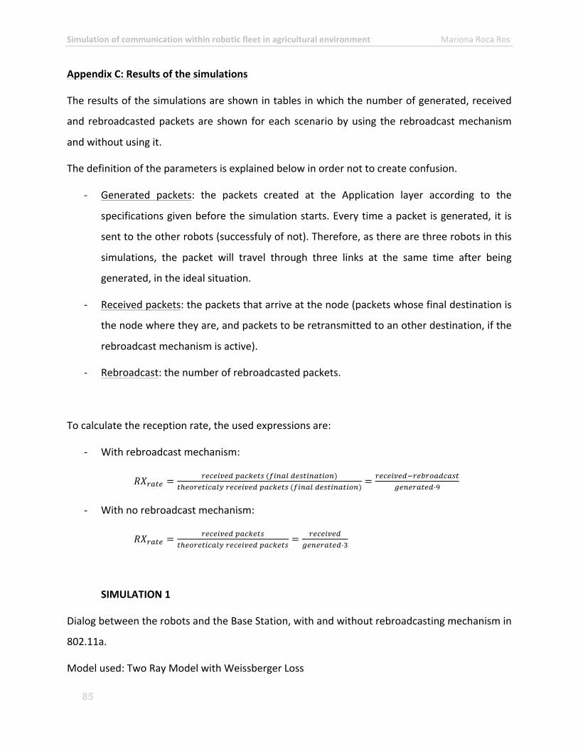
Simulation of communication within robotic fleet in agricultural environment Mariona Roca Ros
85
Appendix C: Results of the simulations
The results of the simulations are shown in tables in which the number of generated, received
and rebroadcasted packets are shown for each scenario by using the rebroadcast mechanism
and without using it.
The definition of the parameters is explained below in order not to create confusion.
-‐ Generated packets: the packets created at the Application layer according to the
specifications given before the simulation starts. Every time a packet is generated, it is
sent to the other robots (successfuly of not). Therefore, as there are three robots in this
simulations, the packet will travel through three links at the same time after being
generated, in the ideal situation.
-‐ Received packets: the packets that arrive at the node (packets whose final destination is
the node where they are, and packets to be retransmitted to an other destination, if the
rebroadcast mechanism is active).
-‐ Rebroadcast: the number of rebroadcasted packets.
To calculate the reception rate, the used expressions are:
-‐ With rebroadcast mechanism:
𝑅𝑋!"#$ =!"#"$%"& !"#$%&' (!"#$% !"#$%&'$%(&)
!!!"#!$%&'() !"#"$%"& !"#$%&' (!"#$% !"#$%&'$%(&)= !"#"$%"&!!"#!$%&'%()
!"#"$%&"'·!
-‐ With no rebroadcast mechanism:
𝑅𝑋!"#$ =!"#"$%"& !"#$%&'
!!!"#!$%&'() !"!"#$"% !"#$%&'= !"#"$%"&
!"#"$%&"'·!
SIMULATION 1
Dialog between the robots and the Base Station, with and without rebroadcasting mechanism in
802.11a.
Model used: Two Ray Model with Weissberger Loss
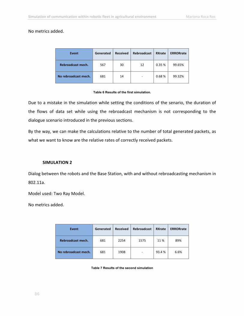
Simulation of communication within robotic fleet in agricultural environment Mariona Roca Ros
86
No metrics added.
Event Generated Received Rebroadcast RXrate ERRORrate
Rebroadcast mech. 567 30 12 0.35 % 99.65%
No rebroadcast mech. 681 14 -‐ 0.68 % 99.32%
Table 6 Results of the first simulation.
Due to a mistake in the simulation while setting the conditions of the senario, the duration of
the flows of data set while using the rebroadcast mechanism is not corresponding to the
dialogue scenario introduced in the previous sections.
By the way, we can make the calculations relative to the number of total generated packets, as
what we want to know are the relative rates of correctly received packets.
SIMULATION 2
Dialog between the robots and the Base Station, with and without rebroadcasting mechanism in
802.11a.
Model used: Two Ray Model.
No metrics added.
Event Generated Received Rebroadcast RXrate ERRORrate
Rebroadcast mech. 681 2254 1575 11 % 89%
No rebroadcast mech. 681 1908 -‐ 93.4 % 6.6%
Table 7 Results of the second simulation
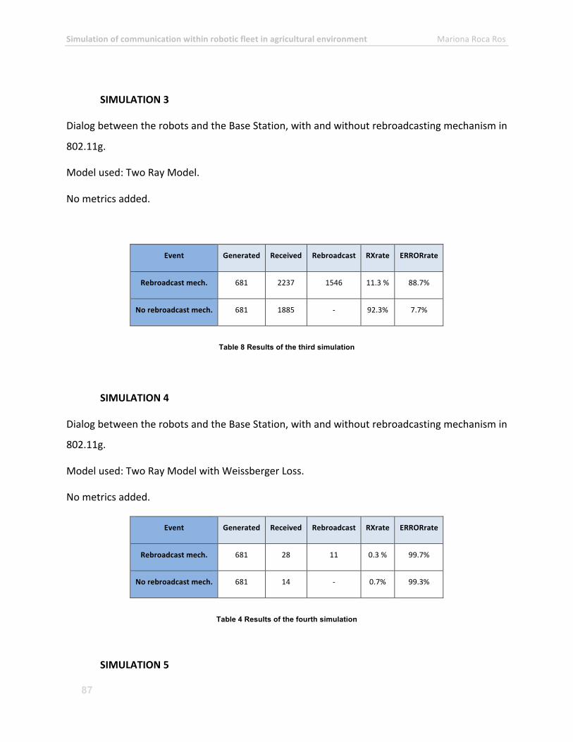
Simulation of communication within robotic fleet in agricultural environment Mariona Roca Ros
87
SIMULATION 3
Dialog between the robots and the Base Station, with and without rebroadcasting mechanism in
802.11g.
Model used: Two Ray Model.
No metrics added.
Event Generated Received Rebroadcast RXrate ERRORrate
Rebroadcast mech. 681 2237 1546 11.3 % 88.7%
No rebroadcast mech. 681 1885 -‐ 92.3% 7.7%
Table 8 Results of the third simulation
SIMULATION 4
Dialog between the robots and the Base Station, with and without rebroadcasting mechanism in
802.11g.
Model used: Two Ray Model with Weissberger Loss.
No metrics added.
Event Generated Received Rebroadcast RXrate ERRORrate
Rebroadcast mech. 681 28 11 0.3 % 99.7%
No rebroadcast mech. 681 14 -‐ 0.7% 99.3%
Table 4 Results of the fourth simulation
SIMULATION 5
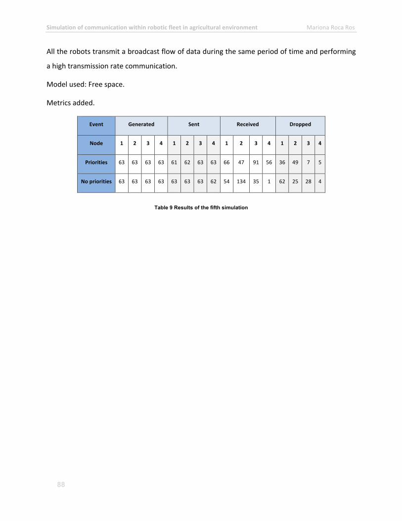
Simulation of communication within robotic fleet in agricultural environment Mariona Roca Ros
88
All the robots transmit a broadcast flow of data during the same period of time and performing
a high transmission rate communication.
Model used: Free space.
Metrics added.
Event Generated Sent Received Dropped
Node 1 2 3 4 1 2 3 4 1 2 3 4 1 2 3 4
Priorities 63 63 63 63 61 62 63 63 66 47 91 56 36 49 7 5
No priorities 63 63 63 63 63 63 63 62 54 134 35 1 62 25 28 4
Table 9 Results of the fifth simulation
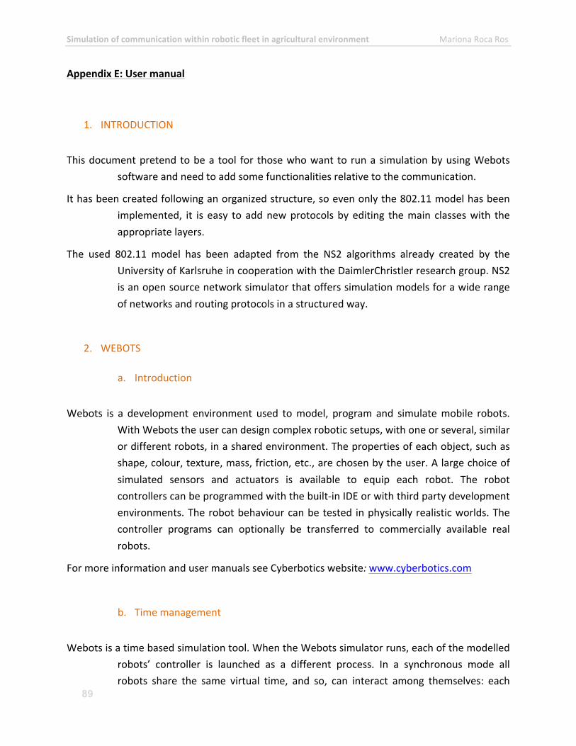
Simulation of communication within robotic fleet in agricultural environment Mariona Roca Ros
89
Appendix E: User manual
1. INTRODUCTION
This document pretend to be a tool for those who want to run a simulation by using Webots software and need to add some functionalities relative to the communication.
It has been created following an organized structure, so even only the 802.11 model has been implemented, it is easy to add new protocols by editing the main classes with the appropriate layers.
The used 802.11 model has been adapted from the NS2 algorithms already created by the University of Karlsruhe in cooperation with the DaimlerChristler research group. NS2 is an open source network simulator that offers simulation models for a wide range of networks and routing protocols in a structured way.
2. WEBOTS
a. Introduction
Webots is a development environment used to model, program and simulate mobile robots. With Webots the user can design complex robotic setups, with one or several, similar or different robots, in a shared environment. The properties of each object, such as shape, colour, texture, mass, friction, etc., are chosen by the user. A large choice of simulated sensors and actuators is available to equip each robot. The robot controllers can be programmed with the built-‐in IDE or with third party development environments. The robot behaviour can be tested in physically realistic worlds. The controller programs can optionally be transferred to commercially available real robots.
For more information and user manuals see Cyberbotics website: www.cyberbotics.com
b. Time management
Webots is a time based simulation tool. When the Webots simulator runs, each of the modelled robots’ controller is launched as a different process. In a synchronous mode all robots share the same virtual time, and so, can interact among themselves: each
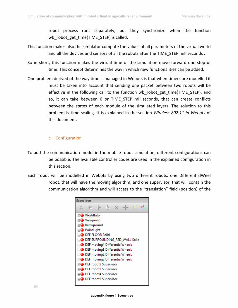
Simulation of communication within robotic fleet in agricultural environment Mariona Roca Ros
90
robot process runs separately, but they synchronize when the function wb_robot_get_time(TIME_STEP) is called.
This function makes also the simulator compute the values of all parameters of the virtual world and all the devices and sensors of all the robots after the TIME_STEP milliseconds .
So in short, this function makes the virtual time of the simulation move forward one step of time. This concept determines the way in which new functionalities can be added.
One problem derived of the way time is managed in Webots is that when timers are modelled it must be taken into account that sending one packet between two robots will be effective in the following call to the function wb_robot_get_time(TIME_STEP), and so, it can take between 0 or TIME_STEP milliseconds, that can create conflicts between the states of each module of the simulated layers. The solution to this problem is time scaling. It is explained in the section Wireless 802.11 in Webots of this document.
c. Configuration
To add the communication model in the mobile robot simulation, different configurations can be possible. The available controller codes are used in the explained configuration in this section.
Each robot will be modelled in Webots by using two different robots: one DifferentialWeel robot, that will have the moving algorithm, and one supervisor, that will contain the communication algorithm and will access to the “translation” field (position) of the
appendix figure 1 Scene tree
Simulation of communication within robotic fleet in agricultural environment Mariona Roca Ros
91
DifferentialWeel, and will use it to calculate some parameters like received Power.
Each modelled robot will have one identifier. It will be a number between 1 and “numrobots” (field described in the annexed table 1).
In the example seen in figure 1, four robots are displayed in the simulation. So for example, for the robot number 1, a Supervisor (robot1) and a DifferentialWheels (moving1) is created.
It is important to follow the structure of the names in the nodes. Otherwise, the controller of each robot will not recognise the devices and no communication will be possible within the different robots.
Notice that the names explained before (moving1 and robot1) are DEF names. These names have nothing to do with the field “name” inside each node. DEF node can be set by clicking the node and writing it at the bottom of the scene tree window.
In the two subsections below both robots are detailed.
“movingX” DifferentialWheels
The only thing to take into account at the moment of creating this robot is its DEF name. This must be “movingX”, where X is the number of the node.
“robotX” Supervisor
In the supervisor there are more things to take into account:
1) The DEF name and the name field of the robot must be set to “robotX”, where X is the number of the robot.
2) The controller of the robot must be the “RHEA_transceiver_X”. Each controller has the value “NUMNODE” set to the number of the robot (1, 2, 3, ...) in the file declare.h.
3) In the children node, two devices must be added: an Emitter and a Receiver (see figures 9 and 10 in the annex) -‐ Emitter:
o Must have its DEF name set to “robotX_emitter”, where X is the number of the robot.
o Type must be set to “radio”
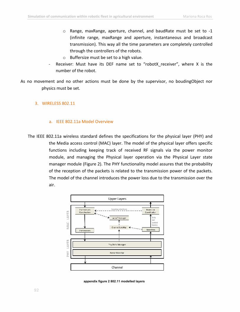
Simulation of communication within robotic fleet in agricultural environment Mariona Roca Ros
92
o Range, maxRange, aperture, channel, and baudRate must be set to -‐1 (infinite range, maxRange and aperture, instantaneous and broadcast transmission). This way all the time parameters are completely controlled through the controllers of the robots.
o Buffersize must be set to a high value. -‐ Receiver: Must have its DEF name set to “robotX_receiver”, where X is the
number of the robot.
As no movement and no other actions must be done by the supervisor, no boudingObject nor physics must be set.
3. WIRELESS 802.11
a. IEEE 802.11a Model Overview
The IEEE 802.11a wireless standard defines the specifications for the physical layer (PHY) and the Media access control (MAC) layer. The model of the physical layer offers specific functions including keeping track of received RF signals via the power monitor module, and managing the Physical layer operation via the Physical Layer state manager module (Figure 2). The PHY functionality model assures that the probability of the reception of the packets is related to the transmission power of the packets. The model of the channel introduces the power loss due to the transmission over the air.
appendix figure 2 802.11 modelled layers
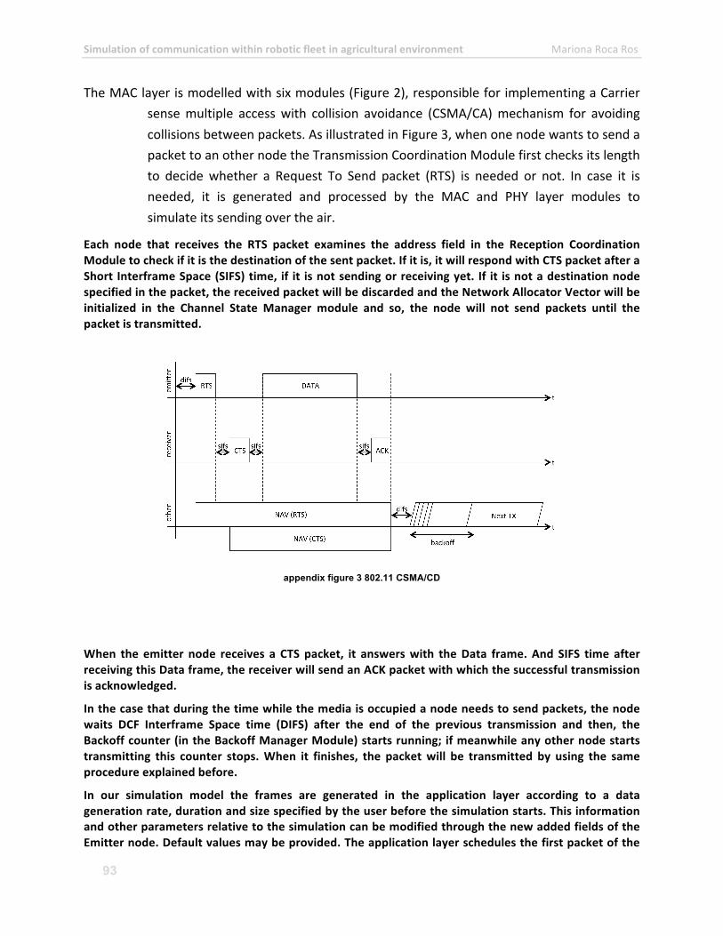
Simulation of communication within robotic fleet in agricultural environment Mariona Roca Ros
93
The MAC layer is modelled with six modules (Figure 2), responsible for implementing a Carrier sense multiple access with collision avoidance (CSMA/CA) mechanism for avoiding collisions between packets. As illustrated in Figure 3, when one node wants to send a packet to an other node the Transmission Coordination Module first checks its length to decide whether a Request To Send packet (RTS) is needed or not. In case it is needed, it is generated and processed by the MAC and PHY layer modules to simulate its sending over the air.
Each node that receives the RTS packet examines the address field in the Reception Coordination Module to check if it is the destination of the sent packet. If it is, it will respond with CTS packet after a Short Interframe Space (SIFS) time, if it is not sending or receiving yet. If it is not a destination node specified in the packet, the received packet will be discarded and the Network Allocator Vector will be initialized in the Channel State Manager module and so, the node will not send packets until the packet is transmitted.
appendix figure 3 802.11 CSMA/CD
When the emitter node receives a CTS packet, it answers with the Data frame. And SIFS time after receiving this Data frame, the receiver will send an ACK packet with which the successful transmission is acknowledged.
In the case that during the time while the media is occupied a node needs to send packets, the node waits DCF Interframe Space time (DIFS) after the end of the previous transmission and then, the Backoff counter (in the Backoff Manager Module) starts running; if meanwhile any other node starts transmitting this counter stops. When it finishes, the packet will be transmitted by using the same procedure explained before.
In our simulation model the frames are generated in the application layer according to a data generation rate, duration and size specified by the user before the simulation starts. This information and other parameters relative to the simulation can be modified through the new added fields of the Emitter node. Default values may be provided. The application layer schedules the first packet of the
Simulation of communication within robotic fleet in agricultural environment Mariona Roca Ros
94
first flow, and the first packet of the other flows are stored in a Queue List from where the MAC layer will pick the packets up when possible.
When a packet is received through the Webots emitter/receiver devices, it is sent to the scheduler and when it is time to, it is attended by the physical layer according to the 802.11 protocol.
b. Configuration and Parameters
The user must introduce the parameters related to the different flows of data involved in the simulation and also the ones making reference to the 802.11 model itself. For the latest, default values have been provided according to the parameters given by the research group who developed the used model for NS2. These values belong with IEEE 802.11a version.
In the annexed table 1, parameters are described with its corresponding default values.
All these parameters must be introduced through the Webots interface. For it, the default “Emitter” node has been modified and must be allocated in the correct folder in the user’s computer. In the folder “\Webots\resources\nodes” the file “emitter.wrl” must be changed by the provided in the pack. Once changed, when Webots simulator is launched, the new fields will appear in the Emitter node, at the scene tree.
Before starting the simulation, other parameters must be also changed, but this time, in the code:
-‐ In each controller “RHEA_transceiver_X.cc”: we must specify the number of the node (NUMNODE) and we must also change the X at the file name (must coincide with the NUMNODE number).
/******************** to be set by the user:***************************************/
/* */
/* must indicate the number of this supervisor in the following define: */
#define NUMNODE 5
/* */
/**********************************************************************************/
-‐ In file “declare.h”, the following parameters must be set: /******************** to be set by the user: **************************************/
/* */
/* speed of the simulation: */
#define TIME_STEP 1 //milliseconds
#define SCALE 6500
/* Two Ray Propagation Model: */
#define PERMITIVITY_ 27
/* if metrics, number of packet types: */
#define NUM_PRI 2 //modify also in R_pack.h
/* if metrics, the priority limits are the following: */
#define LIM0_0 0.0010
#define LIM0_1 0.0011
Simulation of communication within robotic fleet in agricultural environment Mariona Roca Ros
95
#define LIM1_0 0.00000001
#define LIM1_1 0.00000002
/* size of RTS, CTS and ACK. */
#define RTSlen 20 //bytes
#define CTSlen 14
#define ACKlen 14
/* if RHEA application */
#define SLOT_UTILIZATION 80 //0 -‐ 100 (%)
/* Weissberger propagation model. Distance factors: (D1.1 page 97/102) */
#define WEISSBERGER_FACTOR_Z 0.286 //2/7
#define WEISSBERGER_FACTOR_X 0.5 //2/4
/* */
/**********************************************************************************/
-‐ In the case of introducing metrics, the number of packet types must also be introduced in the file R_pack.h:
/******************** to be set by the user:***************************************/
/* */
#define NUM_PRI 2 //also in declare.h
/* */
/**********************************************************************************/
4. WIRELESS 802.11 IN WEBOTS
a. Class and layer structures
As shown in Figure 3, new implemented layers are the PHY and MAC layers corresponding to the structure of the wireless IEEE 802.11a standard and a simple application layer. A pre-‐reception layer is added to simulate the Wireless Channel.
A Queue List is implemented as an interface for the MAC layer, so just one packet is processed at any time while others are in the queue. The mecanism of picking new packets up from this Queue List is implemented in the MAC layer.
Before starting the simulation, the user must fill some parameters regarding to the 802.11 model and the simulation. More information about these parameters in 3b section in this paper.
The layers in our implementation are centrally managed by the Mobilenode object which inherits from a scheduler class that manages how the time evolves. In this approach after a packet is processed by one layer it is put into the scheduler queue. The scheduler takes the packet from the queue according to the time predefined by the last layer which processed the packet and forwards it to the next layer. This way of operation is essential for the implementation of protocols at different layers as the operation of each layer protocol is modeled as a state-‐event machine. In this way the delay that different layers introduce can also be modeled in the simulation to make it more realistic.
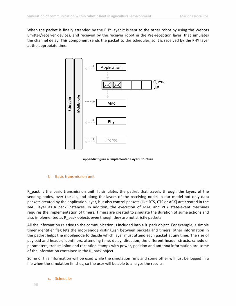
Simulation of communication within robotic fleet in agricultural environment Mariona Roca Ros
96
When the packet is finally attended by the PHY layer it is sent to the other robot by using the Webots Emitter/receiver devices, and received by the receiver robot in the Pre-‐reception layer, that simulates the channel delay. This component sends the packet to the scheduler, so it is received by the PHY layer at the appropiate time.
appendix figure 4 Implemented Layer Structure
b. Basic transmission unit
R_pack is the basic transmission unit. It simulates the packet that travels through the layers of the sending nodes, over the air, and along the layers of the receiving node. In our model not only data packets created by the application layer, but also control packets (like RTS, CTS or ACK) are created in the MAC layer as R_pack instances. In addition, the execution of MAC and PHY state-‐event machines requires the implementation of timers. Timers are created to simulate the duration of sume actions and also implemented as R_pack objects even though they are not strictly packets.
All the information relative to the communication is included into a R_pack object. For example, a simple timer identifier flag lets the mobilenode distinguish between packets and timers; other information in the packet helps the mobilenode to decide which layer must attend each packet at any time. The size of payload and header, identifiers, attending time, delay, direction, the different header structs, scheduler parameters, transmission and reception stamps with power, position and antenna information are some of the information contained in the R_pack object.
Some of this information will be used while the simulation runs and some other will just be logged in a file when the simulation finishes, so the user will be able to analyse the results.
c. Scheduler
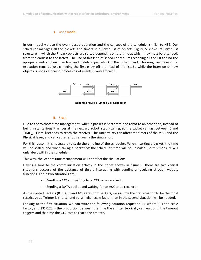
Simulation of communication within robotic fleet in agricultural environment Mariona Roca Ros
97
i. Used model
In our model we use the event-‐based operation and the concept of the scheduler similar to NS2. Our scheduler manages all the packets and timers in a linked list of objects. Figure 5 shows its linked-‐list structure in which the R_pack objects are sorted depending on the time at which they must be attended, from the earliest to the lattest. The use of this kind of scheduler requires scanning all the list to find the apropiate entry when inserting and deleting packets. On the other hand, choosing next event for execution requires just trimming the first entry off the head of the list. So while the insertion of new objects is not so efficient, processing of events is very efficient.
appendix figure 5 Linked List Scheduler
ii. Scale
Due to the Webots time management, when a packet is sent from one robot to an other one, instead of being instantanious it arrives at the next wb_robot_step() calling, so the packet can last between 0 and TIME_STEP milliseconds to reach the receiver. This uncertainty can affect the timers of the MAC and the Physical layer, and can cause serious errors in the simulation.
For this reason, it is necessary to scale the timeline of the scheduler. When inserting a packet, the time will be scaled, and when taking a packet off the scheduler, time will be unscaled. So this measure will only afect within the scheduler.
This way, the webots time management will not afect the simulations.
Having a look to the communication activity in the nodes shown in figure 6, there are two critical situations because of the existance of timers interacting with sending a receiving through webots functions. These two situations are:
-‐ Sending a RTS and waiting for a CTS to be received.
-‐ Sending a DATA packet and waiting for an ACK to be received.
As the control packets (RTS, CTS and ACK) are short packets, we assume the first situation to be the most restrictive as Txtimer is shorter and so, a higher scale factor than in the second situation will be needed.
Looking at the first situation, we can write the following equation (equation 1), where S is the scale factor, and 132/122 is the proportion between the time the emitter teorically can wait until the timeout triggers and the time the CTS lasts to reach the emitter.
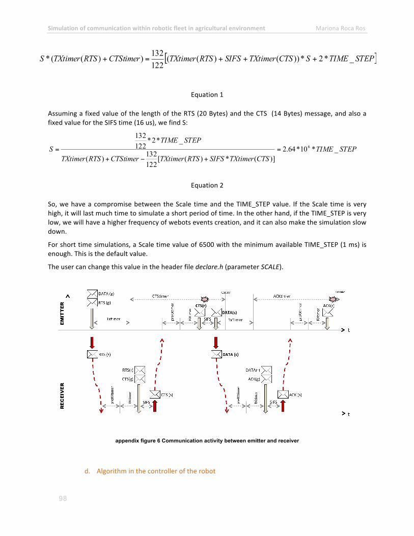
Simulation of communication within robotic fleet in agricultural environment Mariona Roca Ros
98
[ ]STEPTIMESCTSTXtimerSIFSRTSTXtimerCTStimerRTSTXtimerS _*2*))()((122132))((* +++=+
Equation 1
Assuming a fixed value of the length of the RTS (20 Bytes) and the CTS (14 Bytes) message, and also a fixed value for the SIFS time (16 us), we find S:
STEPTIMECTSTXtimerSIFSRTSTXtimerCTStimerRTSTXtimer
STEPTIMES _*10*64.2
)](*)([122132)(
_*2*122132
6=+−+
=
Equation 2
So, we have a compromise between the Scale time and the TIME_STEP value. If the Scale time is very high, it will last much time to simulate a short period of time. In the other hand, if the TIME_STEP is very low, we will have a higher frequency of webots events creation, and it can also make the simulation slow down.
For short time simulations, a Scale time value of 6500 with the minimum available TIME_STEP (1 ms) is enough. This is the default value.
The user can change this value in the header file declare.h (parameter SCALE).
appendix figure 6 Communication activity between emitter and receiver
d. Algorithm in the controller of the robot
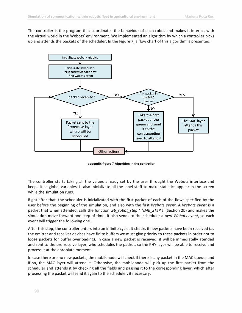
Simulation of communication within robotic fleet in agricultural environment Mariona Roca Ros
99
The controller is the program that coordinates the behaviour of each robot and makes it interact with the virtual world in the Webots’ environment. We implemented an algorithm by which a controller picks up and attends the packets of the scheduler. In the Figure 7, a flow chart of this algorithm is presented.
appendix figure 7 Algorithm in the controller
The controller starts taking all the values already set by the user throught the Webots interface and keeps it as global variables. It also inicializate all the label staff to make statistics appear in the screen while the simulation runs.
Right after that, the scheduler is inicializated with the first packet of each of the flows specified by the user before the beginning of the simulation, and also with the first Webots event. A Webots event is a packet that when attended, calls the function wb_robot_step ( TIME_STEP ) (Section 2b) and makes the simulation move forward one step of time. It also sends to the scheduler a new Webots event, so each event will trigger the following one.
After this step, the controller enters into an infinite cycle. It checks if new packets have been received (as the emitter and receiver devices have finite buffers we must give priority to these packets in order not to loose packets for buffer overloading). In case a new packet is received, it will be inmediatelly atended and sent to the pre-‐receive layer, who schedules the packet, so the PHY layer will be able to receive and process it at the apropiate moment.
In case there are no new packets, the mobilenode will check if there is any packet in the MAC queue, and if so, the MAC layer will attend it. Otherwise, the mobilenode will pick up the first packet from the scheduler and attends it by checking all the fields and passing it to the corresponding layer, which after processing the packet will send it again to the scheduler, if necessary.
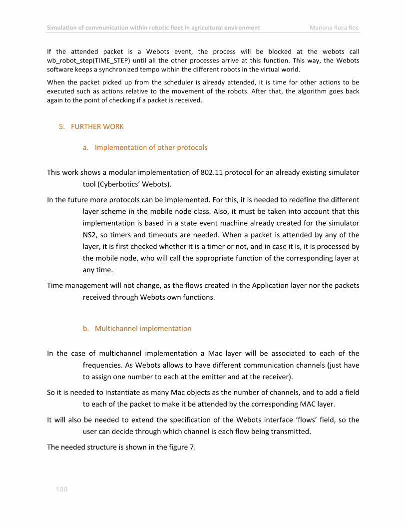
Simulation of communication within robotic fleet in agricultural environment Mariona Roca Ros
100
If the attended packet is a Webots event, the process will be blocked at the webots call wb_robot_step(TIME_STEP) until all the other processes arrive at this function. This way, the Webots software keeps a synchronized tempo within the different robots in the virtual world.
When the packet picked up from the scheduler is already attended, it is time for other actions to be executed such as actions relative to the movement of the robots. After that, the algorithm goes back again to the point of checking if a packet is received.
5. FURTHER WORK
a. Implementation of other protocols
This work shows a modular implementation of 802.11 protocol for an already existing simulator tool (Cyberbotics’ Webots).
In the future more protocols can be implemented. For this, it is needed to redefine the different layer scheme in the mobile node class. Also, it must be taken into account that this implementation is based in a state event machine already created for the simulator NS2, so timers and timeouts are needed. When a packet is attended by any of the layer, it is first checked whether it is a timer or not, and in case it is, it is processed by the mobile node, who will call the appropriate function of the corresponding layer at any time.
Time management will not change, as the flows created in the Application layer nor the packets received through Webots own functions.
b. Multichannel implementation
In the case of multichannel implementation a Mac layer will be associated to each of the frequencies. As Webots allows to have different communication channels (just have to assign one number to each at the emitter and at the receiver).
So it is needed to instantiate as many Mac objects as the number of channels, and to add a field to each of the packet to make it be attended by the corresponding MAC layer.
It will also be needed to extend the specification of the Webots interface ‘flows’ field, so the user can decide through which channel is each flow being transmitted.
The needed structure is shown in the figure 7.
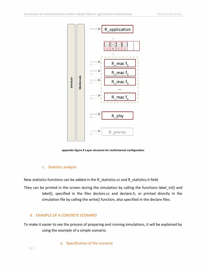
Simulation of communication within robotic fleet in agricultural environment Mariona Roca Ros
101
appendix figure 8 Layer structure for multichannel configuration
c. Statistics analysis
New statistics functions can be added in the R_statistics.cc and R_statistics.h field.
They can be printed in the screen during the simulation by calling the functions label_ini() and label(), specified in the files declare.cc and declare.h, or printed directly in the simulation file by calling the write() function, also specified in the declare files.
6. EXAMPLE OF A CONCRETE SCENARIO
To make it easier to see the process of preparing and running simulations, it will be explained by using the example of a simple scenario.
a. Specification of the scenario
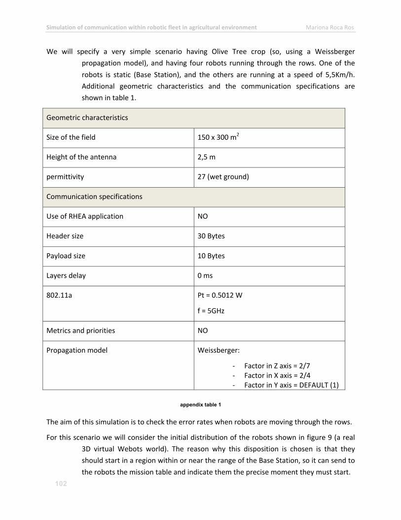
Simulation of communication within robotic fleet in agricultural environment Mariona Roca Ros
102
We will specify a very simple scenario having Olive Tree crop (so, using a Weissberger propagation model), and having four robots running through the rows. One of the robots is static (Base Station), and the others are running at a speed of 5,5Km/h. Additional geometric characteristics and the communication specifications are shown in table 1.
Geometric characteristics
Size of the field 150 x 300 m2
Height of the antenna 2,5 m
permittivity 27 (wet ground)
Communication specifications
Use of RHEA application NO
Header size 30 Bytes
Payload size 10 Bytes
Layers delay 0 ms
802.11a Pt = 0.5012 W
f = 5GHz
Metrics and priorities NO
Propagation model Weissberger:
-‐ Factor in Z axis = 2/7 -‐ Factor in X axis = 2/4 -‐ Factor in Y axis = DEFAULT (1)
appendix table 1
The aim of this simulation is to check the error rates when robots are moving through the rows.
For this scenario we will consider the initial distribution of the robots shown in figure 9 (a real 3D virtual Webots world). The reason why this disposition is chosen is that they should start in a region within or near the range of the Base Station, so it can send to the robots the mission table and indicate them the precise moment they must start.
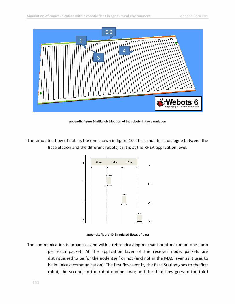
Simulation of communication within robotic fleet in agricultural environment Mariona Roca Ros
103
appendix figure 9 initial distribution of the robots in the simulation
The simulated flow of data is the one shown in figure 10. This simulates a dialogue between the Base Station and the different robots, as it is at the RHEA application level.
appendix figure 10 Simulated flows of data
The communication is broadcast and with a rebroadcasting mechanism of maximum one jump per each packet. At the application layer of the receiver node, packets are distinguished to be for the node itself or not (and not in the MAC layer as it uses to be in unicast communication). The first flow sent by the Base Station goes to the first robot, the second, to the robot number two; and the third flow goes to the third
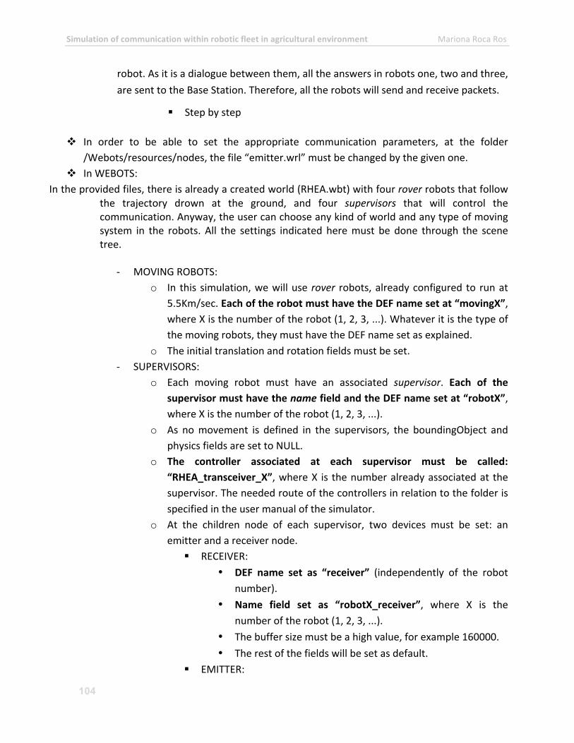
Simulation of communication within robotic fleet in agricultural environment Mariona Roca Ros
104
robot. As it is a dialogue between them, all the answers in robots one, two and three, are sent to the Base Station. Therefore, all the robots will send and receive packets.
§ Step by step
v In order to be able to set the appropriate communication parameters, at the folder /Webots/resources/nodes, the file “emitter.wrl” must be changed by the given one.
v In WEBOTS: In the provided files, there is already a created world (RHEA.wbt) with four rover robots that follow
the trajectory drown at the ground, and four supervisors that will control the communication. Anyway, the user can choose any kind of world and any type of moving system in the robots. All the settings indicated here must be done through the scene tree.
-‐ MOVING ROBOTS:
o In this simulation, we will use rover robots, already configured to run at 5.5Km/sec. Each of the robot must have the DEF name set at “movingX”, where X is the number of the robot (1, 2, 3, ...). Whatever it is the type of the moving robots, they must have the DEF name set as explained.
o The initial translation and rotation fields must be set. -‐ SUPERVISORS:
o Each moving robot must have an associated supervisor. Each of the supervisor must have the name field and the DEF name set at “robotX”, where X is the number of the robot (1, 2, 3, ...).
o As no movement is defined in the supervisors, the boundingObject and physics fields are set to NULL.
o The controller associated at each supervisor must be called: “RHEA_transceiver_X”, where X is the number already associated at the supervisor. The needed route of the controllers in relation to the folder is specified in the user manual of the simulator.
o At the children node of each supervisor, two devices must be set: an emitter and a receiver node.
§ RECEIVER: • DEF name set as “receiver” (independently of the robot
number). • Name field set as “robotX_receiver”, where X is the
number of the robot (1, 2, 3, ...). • The buffer size must be a high value, for example 160000. • The rest of the fields will be set as default.
§ EMITTER:
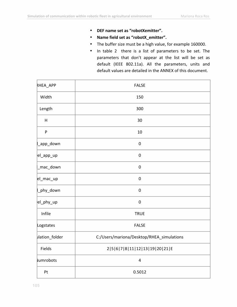
Simulation of communication within robotic fleet in agricultural environment Mariona Roca Ros
105
• DEF name set as “robotXemitter”. • Name field set as “robotX_emitter”. • The buffer size must be a high value, for example 160000. • In table 2 there is a list of parameters to be set. The
parameters that don’t appear at the list will be set as default (IEEE 802.11a). All the parameters, units and default values are detailed in the ANNEX of this document.
RHEA_APP FALSE
Width 150
Length 300
H 30
P 10
Del_app_down 0
Del_app_up 0
Del_mac_down 0
Del_mac_up 0
Del_phy_down 0
Del_phy_up 0
Infile TRUE
Logstates FALSE
Simulation_folder C:/Users/mariona/Desktop/RHEA_simulations
Fields 2|5|6|7|8|11|12|13|19|20|21|E
Numrobots 4
Pt 0.5012
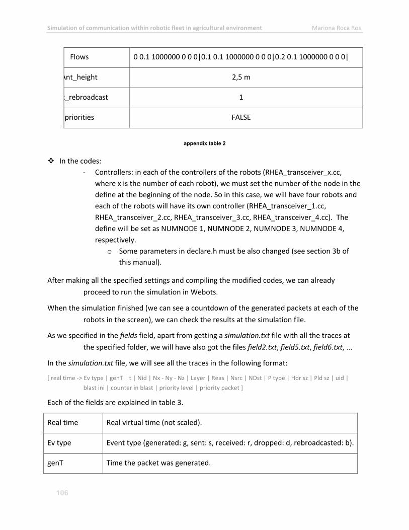
Simulation of communication within robotic fleet in agricultural environment Mariona Roca Ros
106
Flows 0 0.1 1000000 0 0 0|0.1 0.1 1000000 0 0 0|0.2 0.1 1000000 0 0 0|
Ant_height 2,5 m
Max_rebroadcast 1
priorities FALSE
appendix table 2
v In the codes: -‐ Controllers: in each of the controllers of the robots (RHEA_transceiver_x.cc,
where x is the number of each robot), we must set the number of the node in the define at the beginning of the node. So in this case, we will have four robots and each of the robots will have its own controller (RHEA_transceiver_1.cc, RHEA_transceiver_2.cc, RHEA_transceiver_3.cc, RHEA_transceiver_4.cc). The define will be set as NUMNODE 1, NUMNODE 2, NUMNODE 3, NUMNODE 4, respectively.
o Some parameters in declare.h must be also changed (see section 3b of this manual).
After making all the specified settings and compiling the modified codes, we can already proceed to run the simulation in Webots.
When the simulation finished (we can see a countdown of the generated packets at each of the robots in the screen), we can check the results at the simulation file.
As we specified in the fields field, apart from getting a simulation.txt file with all the traces at the specified folder, we will have also got the files field2.txt, field5.txt, field6.txt, ...
In the simulation.txt file, we will see all the traces in the following format:
[ real time -‐> Ev type | genT | t | Nid | Nx -‐ Ny -‐ Nz | Layer | Reas | Nsrc | NDst | P type | Hdr sz | Pld sz | uid | blast ini | counter in blast | priority level | priority packet ]
Each of the fields are explained in table 3.
Real time Real virtual time (not scaled).
Ev type Event type (generated: g, sent: s, received: r, dropped: d, rebroadcasted: b).
genT Time the packet was generated.
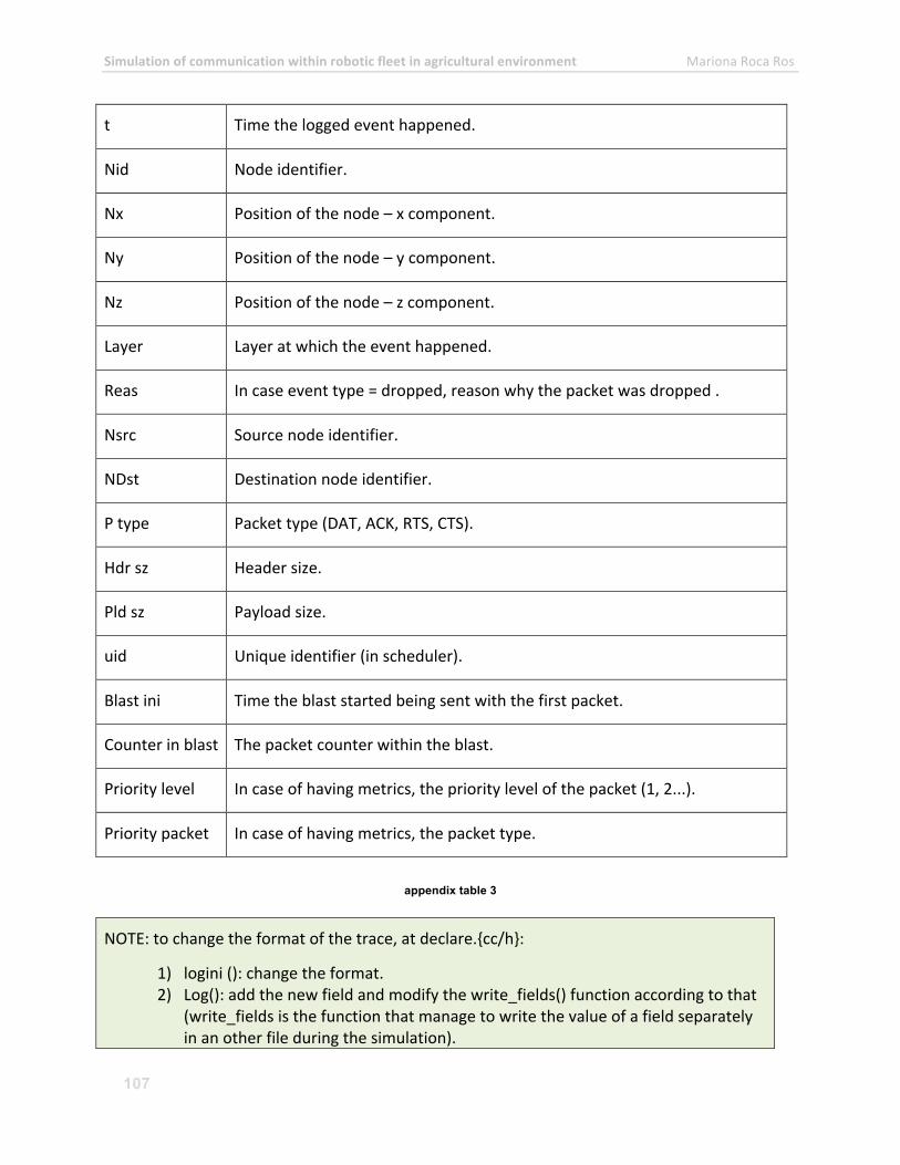
Simulation of communication within robotic fleet in agricultural environment Mariona Roca Ros
107
t Time the logged event happened.
Nid Node identifier.
Nx Position of the node – x component.
Ny Position of the node – y component.
Nz Position of the node – z component.
Layer Layer at which the event happened.
Reas In case event type = dropped, reason why the packet was dropped .
Nsrc Source node identifier.
NDst Destination node identifier.
P type Packet type (DAT, ACK, RTS, CTS).
Hdr sz Header size.
Pld sz Payload size.
uid Unique identifier (in scheduler).
Blast ini Time the blast started being sent with the first packet.
Counter in blast The packet counter within the blast.
Priority level In case of having metrics, the priority level of the packet (1, 2...).
Priority packet In case of having metrics, the packet type.
appendix table 3
NOTE: to change the format of the trace, at declare.{cc/h}:
1) logini (): change the format. 2) Log(): add the new field and modify the write_fields() function according to that
(write_fields is the function that manage to write the value of a field separately in an other file during the simulation).
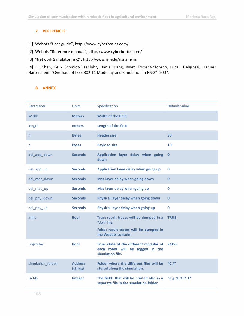
Simulation of communication within robotic fleet in agricultural environment Mariona Roca Ros
108
7. REFERENCES
[1] Webots “User guide”, http://www.cyberbotics.com/
[2] Webots “Reference manual”, http://www.cyberbotics.com/
[3] “Network Simulator ns-‐2”, http://www.isi.edu/nsnam/ns
[4] Qi Chen, Felix Schmidt-‐Eisenlohr, Daniel Jiang, Marc Torrent-‐Moreno, Luca Delgrossi, Hannes Hartenstein, “Overhaul of IEEE 802.11 Modeling and Simulation in NS-‐2“, 2007.
8. ANNEX
Parameter Units Specification Default value
Width Meters Width of the field
length meters Length of the field
h Bytes Header size 30
p Bytes Payload size 10
del_app_down Seconds Application layer delay when going down
0
del_app_up Seconds Application layer delay when going up 0
del_mac_down Seconds Mac layer delay when going down 0
del_mac_up Seconds Mac layer delay when going up 0
del_phy_down Seconds Physical layer delay when going down 0
del_phy_up Seconds Physical layer delay when going up 0
Infile Bool True: result traces will be dumped in a “.txt” file
False: result traces will be dumped in the Webots console
TRUE
Logstates Bool True: state of the different modules of each robot will be logged in the simulation file.
FALSE
simulation_folder Address (string)
Folder where the different files will be stored along the simulation.
"C:/"
Fields Integer The fields that will be printed also in a separate file in the simulation folder.
"e.g. 1|3|7|E"
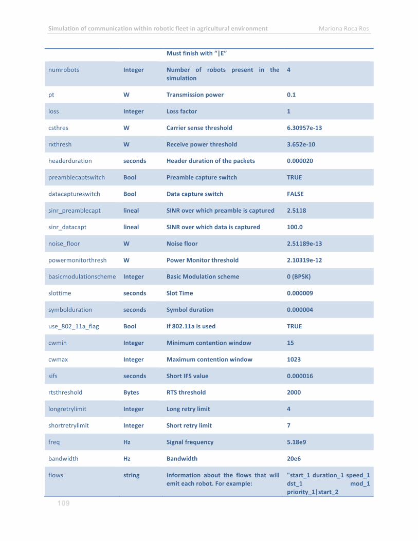
Simulation of communication within robotic fleet in agricultural environment Mariona Roca Ros
109
Must finish with “|E”
numrobots Integer Number of robots present in the simulation
4
pt W Transmission power 0.1
loss Integer Loss factor 1
csthres W Carrier sense threshold 6.30957e-‐13
rxthresh W Receive power threshold 3.652e-‐10
headerduration seconds Header duration of the packets 0.000020
preamblecaptswitch Bool Preamble capture switch TRUE
datacaptureswitch Bool Data capture switch FALSE
sinr_preamblecapt lineal SINR over which preamble is captured 2.5118
sinr_datacapt lineal SINR over which data is captured 100.0
noise_floor W Noise floor 2.51189e-‐13
powermonitorthresh W Power Monitor threshold 2.10319e-‐12
basicmodulationscheme Integer Basic Modulation scheme 0 (BPSK)
slottime seconds Slot Time 0.000009
symbolduration seconds Symbol duration 0.000004
use_802_11a_flag Bool If 802.11a is used TRUE
cwmin Integer Minimum contention window 15
cwmax Integer Maximum contention window 1023
sifs seconds Short IFS value 0.000016
rtsthreshold Bytes RTS threshold 2000
longretrylimit Integer Long retry limit 4
shortretrylimit Integer Short retry limit 7
freq Hz Signal frequency 5.18e9
bandwidth Hz Bandwidth 20e6
flows string Information about the flows that will emit each robot. For example:
"start_1 duration_1 speed_1 dst_1 mod_1 priority_1|start_2
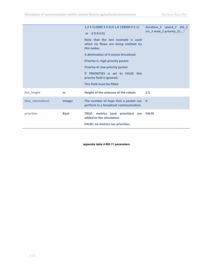
Simulation of communication within robotic fleet in agricultural environment Mariona Roca Ros
110
1,3 4 512000 2 0 0|6 1,8 128000 0 2 1|
or 0 0 0 0 0|
Note that the last example is used when no flows are being emitted by this nodes.
A destination of 0 means Broadcast.
Priority=1: high priority packet
Priority=0: low priority packet
If PRIORITIES is set to FALSE this priority field is ignored.
This field must be filled.
duration_2 speed_2 dst_2 src_2 mod_2 priority_2|..."
Ant_height m Height of the antenna of the robots 2.5
Max_rebroadcast Integer The number of hops that a packet can perform in a broadcast communication.
0
priorities Bool TRUE: metrics (and priorities) are added to the simulation.
FALSE: no metrics nor priorities.
FALSE
appendix table 4 802.11 parameters
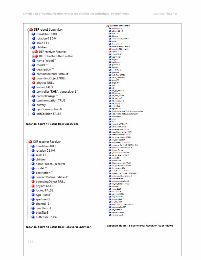
Simulation of communication within robotic fleet in agricultural environment Mariona Roca Ros
111
appendix figure 11 Scene tree: Supervisor
appendix figure 12 Scene tree: Receiver (supervisor)
appendix figure 13 Scene tree: Receiver (supervisor)
Simulation of communication within robotic fleet in agricultural environment Mariona Roca Ros
112
Related Documents