i J:\marginal\FinalDraftReport7-29-99.wpd DRAFT Marginal Energy Prices Report July 1999 U.S. Department of Energy Assistant Secretary, Energy Efficiency & Renewable Energy Office of Codes and Standards Washington, DC 20585

Welcome message from author
This document is posted to help you gain knowledge. Please leave a comment to let me know what you think about it! Share it to your friends and learn new things together.
Transcript
iJ:\marginal\FinalDraftReport7-29-99.wpd
DRAFT
Marginal Energy Prices Report
July 1999
U.S. Department of EnergyAssistant Secretary,Energy Efficiency & Renewable EnergyOffice of Codes and StandardsWashington, DC 20585

iiJ:\marginal\FinalDraftReport7-29-99.wpd
This document was prepared for the Department of Energyby staff members of the
Lawrence Berkeley National Laboratory (LBNL)

iiiJ:\marginal\FinalDraftReport7-29-99.wpd
MARGINAL ENERGY PRICES
Final Report
Page
Outline i
Executive Summary 1
I. Background 2II. Methods 4III. Analysis and Results – Commercial 6IV. Analysis and Results – Residential 12V. Residential Heating Oil and Propane 19VI. Taxes 22
AppendicesAppendix 1. Tariffs Used in the Commercial Analysis 26Appendix 2. Examples of Commercial Bill Calculations 27Appendix 3. Demand Decrement Due to Standards - The Role of Lighting Coincidence and Diversity 28Appendix 4. Weighting Method for Commercial Sample 29Appendix 5. Tax Tables 32
TablesTable 1. Characterization and Summary of Commercial Electric Utility Sample 6Table 2. Distribution of r-squared Values for Electricity (Summer and Winter) and Gas Regressions 14Table 3. Number of Households in Each Appliance Data Set, and in Subsets with Marginal Prices 15Table 4. Heating Oil Prices 19Table 5. Propane Prices 21Table 6. State Sales Taxes 32Table 7. Gas and Electric Utility Regulatory Assessments by States 38Table 8. kWh Taxes on Electricity 38
FiguresFigure 1. Commercial Electricity Marginal Prices 11Figure 2. RECS 1993 Linear Regression on Electricity Bills, Household 4164 13Figure 3. RECS 1993 Linear Regression on Gas Bills, Household 1001 14Figure 4. Residential Summer Electricity Marginal Prices 16Figure 5. Residential Winter Electricity Marginal Prices 17Figure 6. Residential Gas Marginal Prices 18
ContributorsLawrence Berkeley National Laboratory (LBNL) Report Coordinator: Stuart ChaitkinLBNL Report Contributors: Peter Biermayer, Sarah Bretz, Steve Brown, Stuart Chaitkin, Sachu Constantine, Diane Fisher, Sajid Hakim, Lucy Liew, Jim Lutz, Chris Marnay, James E. McMahon, Mithra Moezzi, Julie Osborn, Esther Rawner, Judy Roberson, Greg Rosenquist, Nancy Ryan, Isaac Turiel, Stephen Wiel
Acknowledgments

ivJ:\marginal\FinalDraftReport7-29-99.wpd
This work was prepared for the Assistant Secretary for Energy Efficiency and Renewable Energy, Office of Codes andStandards, of the U.S. Department of Energy, under Contract No. DE-AC03-76SF0098. Data and advice weregraciously provided by Robert Latta and Steve Wade of the Energy Information Administration.

1J:\marginal\FinalDraftReport7-29-99.wpd
MARGINAL ENERGY PRICES – FINAL REPORT
EXECUTIVE SUMMARY
This report responds to a recommendation from the Department of Energy’s (DOE) Advisory Committee on ApplianceEnergy Efficiency Standards. It presents the derivation of estimated consumer marginal energy prices for thecommercial and residential sectors for use in the life-cycle cost (LCC) analyses for four of the high priority appliances’energy efficiency standards rulemakings – clothes washers, water heaters, fluorescent lamp ballasts, and central airconditioners/heat pumps.
Marginal prices as discussed here are those prices consumers pay (or save) for their last units of energy used (orsaved). Marginal prices reflect a change in a consumer’s bill (that might be associated with new energy efficiencystandards) divided by the corresponding change in the amount of energy the consumer used.
Previous LCC analyses had either used Energy Information Administration’s (EIA) Residential Energy ConsumptionSurvey (RECS) household average prices for valuing energy savings from residential sector energy efficiencystandards or a distribution of average prices derived from electric utility data for valuing energy savings fromcommercial sector energy efficiency standards. Average energy prices for a consumer are derived by dividing annualenergy costs by annual energy consumption. At the utility level, average energy prices are derived by dividingannual revenues by annual energy sales.
Section I below provides background on the work developed for marginal energy prices. Section II describes themethods used to derive marginal energy prices. Other credible methods to calculate or estimate consumers’ marginalenergy prices were not found. Because of the complexity inherent in utility tariffs, methods that simply subtract fixedcosts from average costs do not constitute a credible method for calculating marginal prices.
Section III shows the analysis for the commercial sector (for application to fluorescent lamp ballasts). The analysiscentered on the calculation of electricity bills for a distribution of sample buildings in conjunction with a distributionof commercial tariffs. Jackson Associates’ Market Analysis and Information System (MAISY®) database provided thesource of information for the building energy and demand levels among buildings of different types. Commercialtariffs from a sample of utilities were collected and modeled..
Section IV describes the analysis for the residential sector (for application to three products: clothes washers, waterheaters, and central air conditioners/heat pumps). The analysis centered on use of consumer bills from the RECS 1993database. Seasonal marginal electricity prices and annual marginal natural gas prices were derived by calculating theslope of the regression lines associated with monthly bill and consumption data.
Prices of residential heating oil and propane were also examined. Because bills paid by residential consumers for thesefuels are determined almost wholly by the volume purchased, quoted prices are essentially marginal prices. Section Vpresents the results of our examination of residential heating oil and propane prices.
Section VI discusses the effect of taxes on marginal prices.
A summary of the results of the analyses to derive commercial and residential marginal prices follows:
· Commercial- Analysis based on the LBNL/MAISY® approach.- Used tariffs for 21% of national commercial electricity customers.- Electricity marginal prices for individual customers range from 85% below to 51% above the average price
for the same customer. At the consumption-weighted mean of the differences, electricity marginal pricesare 5.2% lower than average prices.
· Residential- Analysis based on the RECS national sample.

1 Letter from Dan Reicher, DOE Assistant Secretary, Energy Efficiency and Renewable Energy, to the AdvisoryCommittee members, July 28, 1998.
2J:\marginal\FinalDraftReport7-29-99.wpd
- Electricity marginal prices for individual customers in the summer (June-September) range from 98%below to 175% above the average price for the same customer. At the consumption-weighted mean ofthe differences, electricity marginal prices are 2.5% higher than average prices in the summer.
- Electricity marginal prices for individual customers in the winter (the remaining eight months) range from100% below to 130% above the average price for the same customer. At the consumption-weightedmean of the differences, electricity marginal prices are 5.3% lower than average prices in the winter.
- Gas marginal prices range for individual customers from 98% below to 248% above the average price forthe same customer. At the consumption-weighted mean of the differences, gas marginal prices are 7.8%lower than average prices.
I. BACKGROUND
The IssueIn the past, DOE’s analyses of the life-cycle costs of and consumer bill savings possible from appliance energyefficiency standards were based on average energy prices. Using marginal energy prices in these analyses is moretheoretically sound because consumers would save energy on the margin (that is, at the price they pay for their lastunit of energy), not at the average price they pay for their energy. Unfortunately, neither published nor readilyavailable data existed for consumer marginal energy prices. Indeed, a major research effort was required to deriveconsumer marginal energy prices.
DOE Advisory CommitteeIn its April 21, 1998 letter to Secretary of Energy Pena, the Advisory Committee on Appliance Energy EfficiencyStandards delivered recommendations to the Department of Energy regarding, among other things, the use of energyprices in future appliance standards rulemakings. For life-cycle cost analyses the Committee recommended that DOEshould replace the use of national average energy prices with the full range of consumer marginal energy rates. Absent consumer marginal energy rate information, the Committee recommended DOE use a range of net energy rates,calculated by removing all fixed charges (such as monthly customer charges that consumers incur regardless of theirmonthly energy usage). In response to the Committee’s recommendations, DOE1 agreed that the use of marginalenergy rates would improve the theoretical soundness of the analysis and decided to determine marginal rates usingeither RECS or commercially available databases. While the Department believed at that time that it was unknown ifremoving fixed costs is more or less reflective of marginal rates, it did not intend to take that intermediate step withoutevidence that the result would improve the accuracy of the analysis.
Fixed ChargesIn considering the recommendation to subtract fixed charges, the Department asked LBNL to examine the dataprovided by the Edison Electric Institute (EEI) concerning electric rates for 104 utilities, serving over 63 millioncustomers. The data included average prices, tail block rates and fixed charges, but not marginal prices. EEI reportedthat fixed charges as a weighted percentage of average prices represent 7.5 percent. However, in examining the actualrate schedules of a few of these 104 utilities, it was found that some of the reported fixed charges were actuallyminimum charges, not customer charges. Thus the actual fixed charges, which are independent of kilowatthour (kWh)usage, would be somewhat lower than the reported 7.5 percent depending upon how often minimum charges wereconsidered to be customer charges within the whole EEI sample of utilities.
The Department agreed that for flat rate schedules, the removal of these adjusted fixed charges would yield themarginal rate. However, upon examining the EEI data, it was determined that most rates are not flat. Of the 104 utilitiesrepresented in the data, 100 contained average price, tail block rate and fixed charges. For utilities with a single flatrate schedule, the average price absent the fixed charges should equal the tail block rate. Of the 100 utilities, only 16met this test within an assumed one percent reporting and rounding error. Thus, 84 percent of the utilities had non-flatrates or a mix of rate schedules which greatly complicates the determination of the marginal price. Of these 84 utilities,

2 MAISY® is a proprietary product that was acquired by LBNL from Jackson Associates, Suite 200, 4825 CreekstoneDrive, Durham, NC 27703; 919-967-9000/919-967-8040 (fax);e-mail:[email protected]
3J:\marginal\FinalDraftReport7-29-99.wpd
roughly half had tail blocks higher than the average price, indicating inclining block rates, and half had lower tailblocks indicating declining block rates. Seasonal rates further complicate this picture.
The American Gas Association (AGA) had conducted a similar analysis using 1996 data for 264 gas utilities serving 46million residential customers. AGA found that fixed customer charges constituted approximately 13.5% of thoseutilities’ total gas revenues from their residential consumers. Beyond noticing that the AGA analysis included onlytwo of California’s gas utilities (e.g., it did not include data for either Pacific Gas & Electric or San Diego Gas &Electric), AGA’s analysis was not closely evaluated.
Marginal PricesWith inclining or declining block rates, the actual value of consumer energy savings is the product of the marginalprice, plus any applicable taxes or fees, times the energy units saved. While simple in theory, the accurate derivationof this saving is very difficult. Consumers are typically billed monthly for their energy usage and will face differentmarginal rates during the year depending on where their energy consumption places them in the rate schedule in anygiven month and how that rate may change with the time of year. It should be noted that just examining the last or tailblock of a rate schedule is not sufficient since many, if not most, consumers do not progress to the last block of therate schedule each and every month of the year. The seasonal variability of appliance usage is most obvious forspace conditioning products such as air conditioners, but, in reality, almost all appliances undergo some seasonalvariation in their usage. Given the possible wide range of marginal prices between winter and summer months, anysignificant seasonal variation in usage could have a significant effect on the marginally calculated savings. Using actual marginal prices may yield consumer energy savings higher or lower than the past method of usingaverage costs based on total revenue. Given the prevalence of summer peaking utilities and seasonal rates, it seemslikely that appliances with heavier summer usage, particularly central air conditioners, would most probably produce agreater consumer value of savings using marginal prices. Therefore, removing fixed costs, which only guaranteeslower estimates of energy prices, would then be a correction in the wrong direction.
RestructuringGiven restructuring of parts of the energy supply sector, customers may soon have more than one bill (e.g., one fromthe distribution company, and one or more from generators or suppliers). To capture complete information, futuresurveys would best gather energy pricing information directly from the customers, rather than from utilities or localdistribution companies. The most efficient means to collect energy pricing information in the future involves includingconsumption by month and pricing information in future bills. The pricing information would include for eachcustomer, the rate schedule: marginal rates, fixed charges, demand charges for commercial and industrial customers, ortime-of-use rates where applicable.
Data SourcesIn the near term (before new surveys can be crafted and implemented), several sources of information were availablefor this current research and analysis on marginal prices. Residential consumers’ utility bills were available from theRECS 1993 survey. Commercial customers’ utility bills could be approximated from monthly usage and likely utilitytariff. Monthly usage for a large sample of commercial buildings was available from a commercial product, theMAISY® commercial database.2 Utility tariff sheets were available from utility web sites, commercial services, or theutilities themselves. Data on utility sales and number of customers on various tariffs were available for investor-owned utilities from the Federal Energy Regulatory Commission (FERC) Form 1 filings made by those utilities. Formunicipal utilities and co-ops, equivalent tariff-level data were obtained from either the utility itself or were availablefrom the Rural Utility Service.

4J:\marginal\FinalDraftReport7-29-99.wpd
II. METHODS
Calculating the true bill effects of proposed appliance energy efficiency standards on diverse U.S. consumers isdifficult because of the many electricity and natural gas tariffs in place, and the complexity of these tariffs. Since theset of end-uses currently under consideration for new standards includes fluorescent lamp ballasts, calculations forcommercial as well as residential electricity customers must be included, which complicates the task considerablybecause commercial tariffs are generally more complex.
To address this difficult research question, several complementary approaches were developed. Those approachesare briefly outlined below. Each of these approaches was a step in the overall sequence of setting up the modelingcapability to allow calculation of samples of customer bills.
“Analytic” ApproachThis approach was the first-cut analysis in which residential electricity and gas tariffs and commercial electricity tariffswere examined as they were collected. Comparing each particular tariff’s rate blocks to average prices yielded themaximum and minimum differences between marginal and average price possible for that particular tariff. Becauseconsumption is unknown, actual customer marginal prices cannot be obtained by this method; only the outer boundsto those prices can be obtained. The findings from this approach were:
a) Care must be taken to find and account for all charges, since the tariffs are often complex, with a numberof charges based on demand levels, voltage levels, seasons, etc. Residential tariffs tend, though, to beless complex than commercial tariffs.
b) For residential gas, individual customer marginal prices are most likely to be below average prices, butwith a large range in results.
c) For residential electricity, individual customer marginal prices can show a very large range, withdifferences ranging from –79% to +344% compared to the average price for customers having a particulartariff, although many of the extreme results appear on tariffs that cover only a few customers and thuswould be seldom experienced.
d) For commercial electricity, individual customer marginal prices also show a large range and no discernablepattern emerged from the analysis.
Because the range of differences between marginal and average prices from this analysis was large, it was concludedthat simple patterns in the relationship between average and marginal prices did not seem to exist. Therefore, thefocus was on the methods that permit estimation of individual customer bills: the experimental, empirical, and RECSanalyses.
“Empirical” ApproachLBNL contracted with Jackson Associates for use of and enhancement to its proprietary MAISY® database of U.S.residential and commercial building energy characteristics. This approach involves allocating these residences andcommercial buildings, currently only identified by state, to electric utility service territories and then to particular utilitytariffs. Monthly customer bills can then be calculated with and without energy and demand savings, yielding marginalprices for each particular consumer. The method and code for conducting the allocation of customers and estimationof bills was developed using two utilities in a southern California test area, and a bill calculator function using theactual tariffs of electric and gas utilities was developed. For commercial buildings, this approach evolved into the oneexplained in Section III. Since an estimate of the effect on the house’s natural gas bill was also required for analysis ofthe three residential products (clothes washers, water heaters, and central air conditioners/heat pumps), thehouseholds were further assigned to a natural gas local distribution company (LDC) that serves a part of the territoryof that residence’s electric utility. While for residential buildings, this “empirical” approach was put aside in favor ofthe RECS approach described below, it was used as the foundation for the “experimental” approach in the analysis ofcommercial sector fluorescent lamp ballasts.
“Experimental” ApproachDuring the collection of tariffs and the designing of the computer code for the empirical approach, a spreadsheet billcalculator was developed. Exploratory experimental tariffs could be modeled in this spreadsheet, and, together with

5J:\marginal\FinalDraftReport7-29-99.wpd
load shapes from the general literature and estimates of monthly customer energy use effects, bills can be estimated. A variation of this method that used actual commercial tariffs and load shapes from MAISY® commercial buildingsprovided the technical approach used for the commercial sector analysis. See Section III for the details and results ofthis method as applied in final form to the analysis of the commercial sector.
“Big Bang” ApproachThe initial sample of electric utility tariffs that was analyzed had been chosen with consideration of diversity in termsof utility ownership, geography, and utility size in mind. That sample was extended, as time permitted, but the utility-by-utility detailed approach necessarily covered only a limited fraction of the total customer population. On the otherhand, a large fraction of customers in the country are actually served on a rather small number of tariffs from a limitednumber of large utilities. This fact suggested an alternative “big bang” approach. In this approach, the tariffs with thegreatest number of customers would be examined. This approach was drawn upon to a limited degree in the expansionof the set of commercial tariffs used in the final commercial sector analysis.
RECS ApproachConsumer marginal energy prices were estimated directly from household RECS data by calculating the slopes of theregression lines that relate customer bills and customer usage. For electricity, the slopes of the regressions for foursummer months (June-September) and, separately, for the remaining (“winter”) months were calculated. For naturalgas, the data did not support calculations beyond the annual level. After exploring the empirical method outlinedabove for use in the analysis for the residential sector, the RECS method (because of its advantages which areexplained further in Section IV) was adopted for the analysis of residential marginal prices in this project. See SectionIV for the details and the results of this RECS method.
Linkage to the Product LCC AnalysesTo anticipate the impact of using marginal prices in place of average prices, a simple sensitivity analysis on the LCCfor each product was conducted, using a range of possible energy price variations. The results were:
a) For central air conditioners, the efficiency level having the minimum LCC was not affected over the range-25 to +25% from average energy prices.
b) For water heaters, the design option for electric water heaters having the minimum life cycle cost issensitive to the value of marginal energy prices, but less so for natural gas water heaters.
c) For clothes washers, the efficiency level having the minimum LCC was not affected over the range –25%to +25% from average energy prices. In addition, payback period was shown to be affected by a lowerpercentage than the change in energy prices, because the operating savings due to water is unaffected bya change in energy price.
d) For ballasts, electronic ballasts were shown to reduce LCC at energy prices down to 45% below average,compared to energy efficient magnetic (EEM). For cathode cutouts, energy prices down to 10% belowaverage still yielded a reduced LCC compared to EEM.
See the relevant Technical Support Documents (TSDs), Notice of Proposed Rulemakings (NOPRs), and the AdvancedNotice of Proposed Rulemaking (ANOPR) – all in progress -- for information on the application of the results of themarginal energy price study to specific products.
6J:\marginal\FinalDraftReport7-29-99.wpd
Utility Sta
te
Typ
e
Cust.MWh Sales Cust.
MWh Sales
PG&E CA IOU 552,901 49,530,911 401,747 16,025,437 3.0% 1.7% 73% 32%SoCal Edison CA IOU 481,417 51,410,408 419,163 23,057,727 3.1% 2.5% 87% 45%Commonwealth Edison IL IOU 292,709 49,933,859 291,143 25,859,649 2.2% 2.8% 99% 52%Virginia Power VA IOU 189,301 20,061,476 137,813 2,696,019 1.0% 0.3% 73% 13%Detroit Edison MI IOU 177,088 17,997,214 166,003 7,613,394 1.2% 0.8% 94% 42%Alabama Power AL IOU 174,602 11,330,312 154,077 7,917,907 1.1% 0.9% 88% 70%Penn Power & Light PA IOU 149,221 20,475,206 143,849 8,781,171 1.1% 0.9% 96% 43%Niagara Mohawk Power NY IOU 148,124 23,279,622 143,590 4,550,295 1.1% 0.5% 97% 20%NSP (MN) MN IOU 135,183 5,009,755 110,807 4,461,852 0.8% 0.5% 82% 89%Union Electric Co MO IOU 134,699 12,189,235 120,596 8,735,132 0.9% 0.9% 90% 72%Appalachian Power VA IOU 110,740 16,390,313 78,554 674,926 0.6% 0.1% 71% 4%Jersey Central P&L NJ IOU 106,157 10,510,309 104,922 5,358,036 0.8% 0.6% 99% 51%Wisconsin Elec Power WI IOU 93,973 18,454,563 85,735 2,705,293 0.6% 0.3% 91% 15%Boston Edison MA IOU 87,644 7,991,349 80,255 2,820,415 0.6% 0.3% 92% 35%Ohio Power Company OH IOU 87,314 24,917,126 6,442 6,348,160 0.0% 0.7% 7% 25%Central Power & Light TX IOU 85,311 12,844,712 74,107 2,099,439 0.5% 0.2% 87% 16%Arizona Public Service AZ IOU 79,755 8,524,882 78,530 6,989,968 0.6% 0.8% 98% 82%PEPCO MD IOU 70,909 15,307,001 53,620 1,317,800 0.4% 0.1% 76% 9%Cleveland Electric Illum OH IOU 64,907 5,883,328 63,161 2,765,339 0.5% 0.3% 97% 47%Seattle City Light WA Muni 43,497 3,081,941 43,497 3,081,941 0.3% 0.3% 100% 100%NSP (WI) WI IOU 31,236 866,425 27,449 831,739 0.2% 0.1% 88% 96%Madison Gas & Electric WI IOU 16,220 1,727,832 14,815 685,233 0.1% 0.1% 91% 40%Savannah Elec & Power GA IOU 14,100 1,156,078 708 517,052 0.0% 0.1% 5% 45%Poudre Valley REA CO Co-op 2,774 377,974 2,101 96,424 0.0% 0.0% 76% 26%
Sample Total 389,251,831 2,802,684 145,990,348 20.7% 15.7% 84% 38%US TOTAL 928,440,265
Percent of US in Modeled Tariffs
Our Sample as Percent of Utility
By Modeled Tariffs By Utility
Cust.Megawatt-hour
Sales
3,329,78213,540,374
Total Number of Customers
Total Megawatt-hour Sales
III. ANALYSIS AND RESULTS – COMMERCIAL
Commercial marginal electricity prices were derived by calculating monthly bills for a distribution of buildings (withenergy usage information) using a set of modeled commercial tariffs. This section of the Marginal Energy Prices reportfirst describes the utility tariffs that were chosen and modeled for this analysis. Then the process for calculating theelectricity bills and the marginal electricity prices for the sampled commercial buildings is described. Becausecommercial tariffs tend to have demand charges, the adjustment applied to represent the reduction in demandassociated with new energy efficiency standards is described next. The method by which the sampled buildings areweighted in the analysis is also described. Lastly, the results of the commercial analysis are presented.
A. Tariff Collection and Modeling
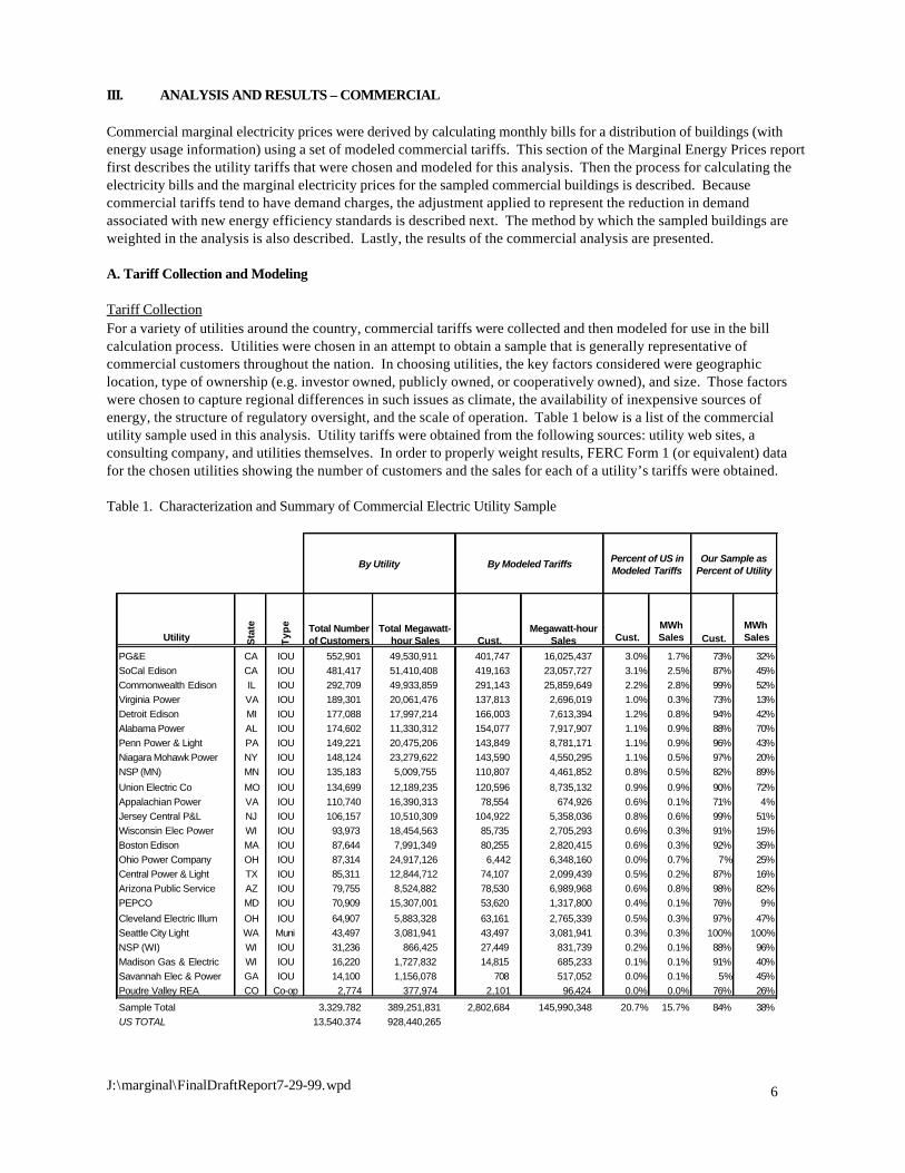
Tariff CollectionFor a variety of utilities around the country, commercial tariffs were collected and then modeled for use in the billcalculation process. Utilities were chosen in an attempt to obtain a sample that is generally representative ofcommercial customers throughout the nation. In choosing utilities, the key factors considered were geographiclocation, type of ownership (e.g. investor owned, publicly owned, or cooperatively owned), and size. Those factorswere chosen to capture regional differences in such issues as climate, the availability of inexpensive sources ofenergy, the structure of regulatory oversight, and the scale of operation. Table 1 below is a list of the commercialutility sample used in this analysis. Utility tariffs were obtained from the following sources: utility web sites, aconsulting company, and utilities themselves. In order to properly weight results, FERC Form 1 (or equivalent) datafor the chosen utilities showing the number of customers and the sales for each of a utility’s tariffs were obtained.
Table 1. Characterization and Summary of Commercial Electric Utility Sample

7J:\marginal\FinalDraftReport7-29-99.wpd
Because tariff-level information on sales is not as readily available for publicly and cooperatively owned utilities as itis for investor-owned utilities that must report such information annually to FERC, the sample contained only onemunicipal utility and one co-op. While the co-op included in the analysis had an average commercial price nearly thesame as the average commercial price of all of the co-ops in the country, the same was not true for the municipal utilityin our sample. As a sensitivity analysis, several more municipal utilities were later added, which brought the weightedaverage electricity price of the municipal utilities in the sample closer to the average commercial price of all of themunicipal utilities in the country. The bill calculator (which is described below) was then re-run using the expandedset of tariffs. See Section D below for the results of this sensitivity analysis.
Commercial Tariff StructureCommercial tariffs can be complex. A commercial tariff usually includes the following types of information:· Applicability / Availability — the type of customer served under this tariff.· Character of Service — the type of current, voltage, and single or three-phase.· Monthly Rate — customer charge, energy charge, demand charge (if applicable), and extra charges.· Definition of demand charges.· Rate periods (if time-of-use) and definition of seasons.· Minimum monthly charge.· Power factor adjustments and reactive power demand charges.
Commercial Spreadsheet ModelingGenerally, the commercial tariff modeling effort focused on two common categories of commercial tariffs: small generalservice and general service. The collected commercial tariffs were modeled in spreadsheet form, excluding some tariffsand/or components that could not be applied to buildings in MAISY®. For instance, some tariffs provide charges forboth single and three-phase service. Because MAISY® does not distinguish between these two types of service, onlythe charges for single phase were modeled. Also, some tariffs charge different prices for primary, secondary, andtransmission voltage levels. Because of the types of buildings used in MAISY®, only the secondary voltage levelswere considered. Power factor and reactive demand charges, which are adjustments based on voltage and demandusage, were ignored. Other factors were ignored if the information could not be used in MAISY® or are rarelyapplicable. The spreadsheet also contains the number of customers in a tariff, total number of customers in acommercial utility, the megawatt-hours sold, kilowatt-hours sold per customer, and average price per kilowatt-hour. These data were extracted from FERC Form 1 for IOU’s and from comparable sources for municipal utilities and co-ops.
B. Calculation of Commercial Bills and Marginal Prices
OverviewThe Commercial Tariffs Spreadsheet, or CTAS, contains a collection of modeled commercial electric utility tariffs, acollection of modeled commercial buildings, and Visual Basic program modules. Each building is assigned to a groupof applicable tariffs, based on building demand, and monthly bills are calculated for each tariff for a calendar year. Then, building energy usage and demands are decremented to account for savings expected from a new energyefficiency standard, monthly bills are recalculated, and the differences in bills and energy use are used to calculatemarginal prices.
Commercial TariffsElectric utilities calculate customer bills from tariffs that define the type and amount of each charge. These charges aregenerally levied on a monthly basis, and generally have three main components: fixed charges, usage charges, anddemand charges. These tariffs were collected for a number of US electric utilities and modeled for inclusion in CTAScalculations. CTAS contains the specific commercial tariffs for the utilities shown in Appendix 1.
In addition to the parameters necessary to calculate customer bills, information was collected for each tariff regardingthe number of customers, revenues, and delivered energy. This tariff-level data on customers and delivered energywere used to weight the resulting bill and marginal price calculations to represent a national distribution of marginalprices. The calculations did not use a tariff unless it was also possible to collect usage and delivered energy data forthat individual tariff (as opposed to being able to collect such information only for the entire utility or a group of that
3 Source: CBECS Table BC-39: Lighting Equipment, Number of Buildings, 1995.
8J:\marginal\FinalDraftReport7-29-99.wpd
utility’s tariffs). Industrial tariffs, as contrasted to commercial tariffs, have not been included in CTAS. This isprimarily because the MAISY® database does not include industrial buildings.
Electric utilities typically have many commercial tariffs. Southern California Edison, for instance, has over 100commercial tariffs. Most of these tariffs target a very small number of customers, or even individual customers, andthus have been ignored in CTAS. To maximize coverage in the limited time available, only the most-used two or threecommercial tariffs for each utility have been included in CTAS. Taken together, these few tariffs cover 84% of thecustomers in our utility sample and 38% of the commercial electricity sales by those sampled utilities.
Generally speaking, commercial customers are assigned to a particular tariff based on their peak monthly and/or annualdemand as measured in kilowatts over a short period of time, e.g. 15 or 30 minutes. This demand “window” was usedto determine which of all the tariffs to apply to a particular building in the CTAS collection. For instance the GS-2 tariffcarried by Southern California Edison is applied to a customer/building whose peak demand is between 20 and 500kW. This assignment by demand window means that a particular building will have bills calculated using some subsetof all the modeled tariffs, typically one tariff per utility.
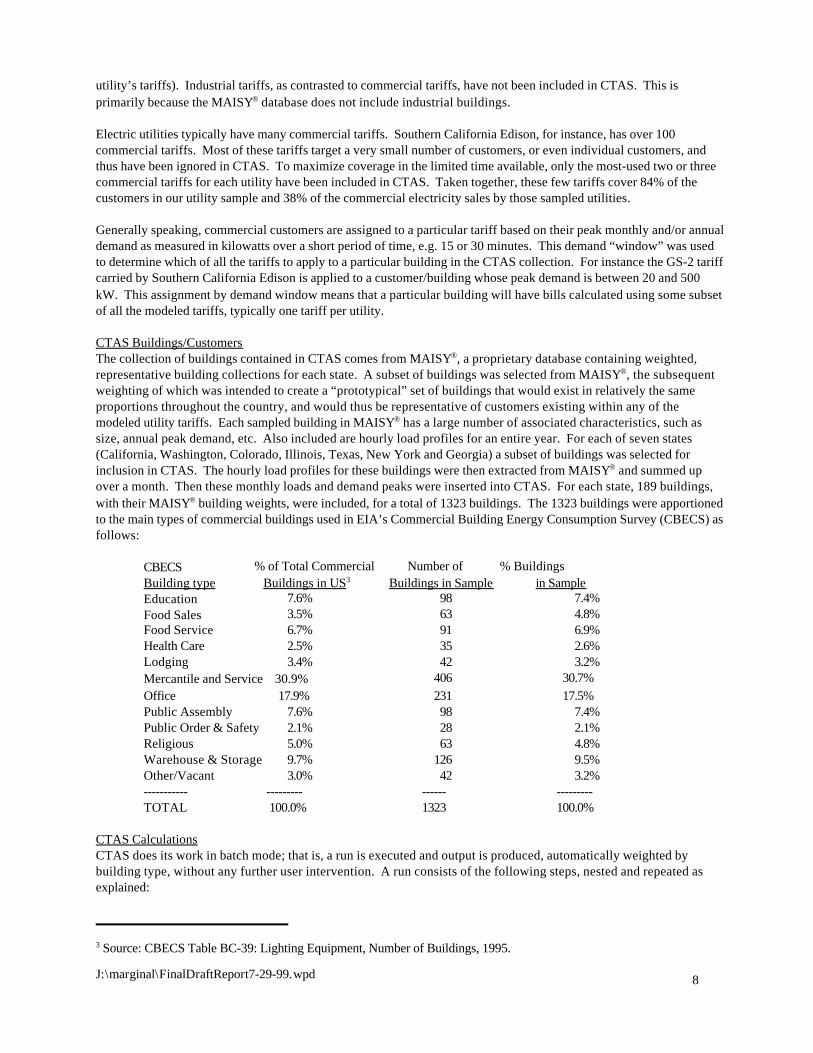
CTAS Buildings/CustomersThe collection of buildings contained in CTAS comes from MAISY®, a proprietary database containing weighted,representative building collections for each state. A subset of buildings was selected from MAISY®, the subsequentweighting of which was intended to create a “prototypical” set of buildings that would exist in relatively the sameproportions throughout the country, and would thus be representative of customers existing within any of themodeled utility tariffs. Each sampled building in MAISY® has a large number of associated characteristics, such assize, annual peak demand, etc. Also included are hourly load profiles for an entire year. For each of seven states(California, Washington, Colorado, Illinois, Texas, New York and Georgia) a subset of buildings was selected forinclusion in CTAS. The hourly load profiles for these buildings were then extracted from MAISY® and summed upover a month. Then these monthly loads and demand peaks were inserted into CTAS. For each state, 189 buildings,with their MAISY® building weights, were included, for a total of 1323 buildings. The 1323 buildings were apportionedto the main types of commercial buildings used in EIA’s Commercial Building Energy Consumption Survey (CBECS) asfollows:
CBECS % of Total Commercial Number of % BuildingsBuilding type Buildings in US3 Buildings in Sample in SampleEducation 7.6% 98 7.4%Food Sales 3.5% 63 4.8%Food Service 6.7% 91 6.9%Health Care 2.5% 35 2.6%Lodging 3.4% 42 3.2%Mercantile and Service 30.9% 406 30.7%Office 17.9% 231 17.5%Public Assembly 7.6% 98 7.4%Public Order & Safety 2.1% 28 2.1%Religious 5.0% 63 4.8%Warehouse & Storage 9.7% 126 9.5%Other/Vacant 3.0% 42 3.2%----------- --------- ------ ---------TOTAL 100.0% 1323 100.0%
CTAS CalculationsCTAS does its work in batch mode; that is, a run is executed and output is produced, automatically weighted bybuilding type, without any further user intervention. A run consists of the following steps, nested and repeated asexplained:

4 See Appendix 2 for sample commercial bill calculations.5 The explanation of the derivation of the demand decrement appears in Appendix 3: “Demand Decrement Due toStandards – The Role of Lighting Coincidence and Diversity.”
9J:\marginal\FinalDraftReport7-29-99.wpd
• Each customer/building is considered in turn.• For each building a selection is made of applicable tariffs, based on that building’s peak annual demand.• For each tariff a calculation of a monthly bill in $/month is performed.4
• A second calculation with the same month, tariff and building is performed with decremented monthly energyuse and peak demand to obtain a representative change in the building’s bill (in order to calculate the marginalenergy price). The assumed energy use decrement is 5%; the demand decrement is 80% of 5%, that is, 4%.5
• A monthly marginal price in $/kWh for this month-tariff-building is computed by dividing the difference betweenthe two bills by the difference between the two energy consumption levels, e.g., change in $/change in kWh.
• An average price in $/kWh is computed by dividing the original, undecremented bill by the original energy use,e.g. bill $/total kWh.
• The percentage difference between the average and marginal price is calculated by subtracting the average pricefrom the marginal price and dividing by the marginal price.
• These calculations are repeated for the 12 months of a calendar year.• Annual values are obtained for average price, marginal price, and percent difference by summing each month’s
values over the year and dividing by 12.• The process is repeated for each applicable tariff for the particular customer/building.• The next building is considered and the complete process repeated, until all customer/buildings have been
processed.
CTAS OutputThe output from a CTAS run is written to a comma-separated-values, or “csv” file, with a record for each building-tariffmatch. This file, containing the fields shown below, is loaded into a FoxPro® table where additional processing occursto produce various charts and distributions.
Field Name Field Description-------------- ----------------------ACCTNO MAISY® customer / building ID numberSTATE State from which sample customer was drawnANPKKW Building annual peak demand in kW measured over 1 hourTARFTYP Tariff group index defined by demand “window”ARFINDX Index used in programTARPTR Index used in programUTILCO Electric utility’s name, e.g. Consolidated EdisonTARFNAME Name of particular tariff, e.g. GS-1NCUS Number of customers billed under that tariffDELVDMWH Annual megawatthours (MWh) delivered by utility to customers under this tariffBLDGWT Calculated weight of building, derived in part from MAISY® weightBLDGOPHRWeekly hours of operation of buildingANAVGRAT Annual average electricity priceANMR1 Annual average electricity marginal priceANE1 Annual percent difference between marginal and average electricity priceAVGBILL Annual average bill, defined as average of 12 monthly billsAVGBILL1 Annual average decremented bill, defined as average of 12 monthly average billsAVGKWH Annual average energy use, defined as average of 12 monthly energy usage levelsAVGKWH1 Annual average decremented energy use, defined as average of 12 monthly decremented energy
usage levels

6 The individual amounts by which average prices exceeded marginal prices had to be binned to prepare inputs for theLCC analysis. The weighted mean of the binned distribution was –5.7%.
10J:\marginal\FinalDraftReport7-29-99.wpd
ConclusionsCTAS was designed as an analysis tool to investigate marginal prices experienced by a range of customers over arange of commercial tariffs throughout the country. It attempts to maximize coverage by running a prototypical set ofcustomers/buildings against as broad a set of tariffs as possible, given the time constraints of the project.
C. Weighting Method
This section describes construction of the weighted distribution of commercial electricity marginal prices. The sampleof commercial buildings consisted of 1323 buildings from seven states with each building supplying multipleobservations to the final data set, one for each applicable tariff. Each observation in the final data set represents aunique combination of a building and an applicable tariff, for a total of 29,133 observations.
The composition of the sample posed a dual weighting problem: distributing weights across buildings and acrosstariffs. The weighting approach solves these problems sequentially. For each building a weight is derived from itsoriginal MAISY® building weight and scaling factors. This adjusted building weight is then apportioned across all thetariffs that were applied to the building. A composite weighting factor for each building/tariff pair combines both ofthese weighting factors. These weights are all based on energy, average monthly kWh usage at the building level andannual MWh sales for each tariff. Appendix 4, Weighting Method for Commercial Sample, shows the details of theapproach to this dual weighting problem.
D. Results of Analysis
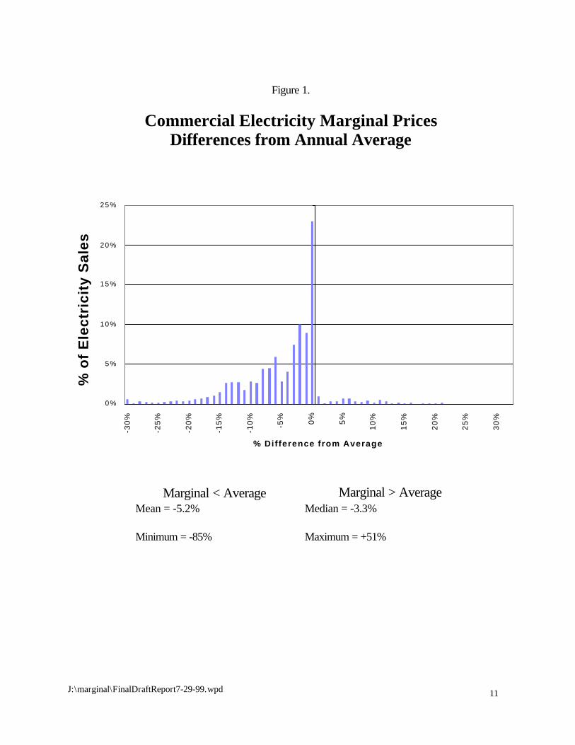
Figure 1 below displays the results of the commercial analysis by showing the distribution of the differences derivedbetween marginal electricity prices and average electricity prices. Electricity marginal prices range from 85% below to51% above the average price for the same customer. At the consumption-weighted mean of the differences, electricitymarginal prices are 5.2% lower than average prices.6 In the LCC analysis of commercial sector ballasts, this distributionof differences was used along with a distribution of average commercial sector electricity prices (which were obtainedfrom EIA data on over 3000 utilities serving commercial customers) to generate a distribution of marginal electricityprices. In the LCC analysis of industrial sector ballasts, this same distribution of differences was used along with adistribution of average industrial sector electricity prices (which were obtained from EIA data on over 2000 utilitiesserving industrial customers) to generate a distribution of marginal electricity prices.
As a result of the sensitivity analysis mentioned earlier (where additional municipal utility tariffs were included), asimilar distribution of weighted amounts were found by which average prices exceeded marginal prices, the mean ofwhich was –5.6%.
11J:\marginal\FinalDraftReport7-29-99.wpd
0%
5%
10%
15%
20%
25%
-30%
-25%
-20%
-15%
-10% -5
% 0% 5%
10%
15%
20%
25%
30%
% Difference from Average
% o
f E
lect
rici
ty S
ales
Figure 1.
Commercial Electricity Marginal PricesDifferences from Annual Average
Marginal < Average Marginal > AverageMean = -5.2% Median = -3.3%
Minimum = -85% Maximum = +51%

7 Source: Robert Latta of EIA proposed this approach.
12J:\marginal\FinalDraftReport7-29-99.wpd
IV. ANALYSIS AND RESULTS – RESIDENTIAL
Method Used to Derive Residential Electric and Natural Gas Marginal PricesData from the Energy Information Administration’s (EIA) 1993 Residential Energy Consumption Survey (RECS) wereused to calculate marginal energy prices for residential appliance owners. The main advantages of using RECS dataare: 1) this survey of 7041 U.S. households was designed by EIA to be a nationally representative sample; and 2) thedata are available to the public. Since RECS includes the exact amounts households paid for utility bills, there is noneed to derive those bills from a combination of an appropriate tariff and each building’s energy consumption. Thus,the method for deriving residential marginal energy prices was inherently simpler than our previously describedmethod for deriving commercial marginal energy prices.
EIA had collected utility bills for up to 16 billing cycles for 6119 of the 7038 RECS households that use electricity, andfor 3153 of the 4033 RECS households that use natural gas. EIA has made a public use version of these data available;it includes some error inoculation to protect the identity of individual utility customers.
Marginal energy prices were calculated by performing a separate regression analysis for each household for whichbilling data were available.7 Energy consumption was plotted on the x-axis, and the consumer’s energy bill was plottedon the y-axis. The slope of the regression line for each household (the change in the energy bill divided by thechange in the energy consumption) equals the marginal energy price for that household.
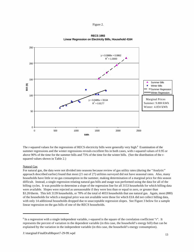
ElectricityFor electricity, the billing data were divided into two seasons, summer and “winter” (actually non-summer), where a billwas defined to be a summer bill if the midpoint of the billing period fell between June 1 and September 30. Thisdivision was done because review of utility tariffs (during the “Analytic” approach described earlier) had found thatelectric utilities often had different rates in summer vs. non-summer, and that most utilities defined summer to fallwithin this range of dates. A linear regression relating electricity bills and usage was performed separately for eachseason. The marginal electricity price for each season was estimated to be equal to the slope of the regression line. See Figure 2 below for a sample linear regression on the electricity bills of one of the RECS households.
For some households, there were either not enough data or the data points were too close together or too scattered todetermine a slope, particularly in the summer season. After a household-by-household examination of the outliers,slopes (marginal prices) that were either less than or equal to zero or greater than $0.22/kWh were also rejected. It waspossible to calculate slopes for the summer season for 5818 households, of which 5615 had acceptable fits, yieldingslopes that fell within the above range of values. It was possible to determine a slope for the “non-summer” seasonfor all 6119 households for which electricity billing data were available. Of these households, 6098 had slopes withacceptable fits. There were a total of 5606 households for which both the summer and non-summer marginal electricityprices could be determined with acceptable fits. Seasonal prices were used for each of these households in the LCCanalysis.
For households for which it was not possible to determine a seasonal rate for both seasons, or for which these ratesfell outside the acceptable range, a single linear regression was performed from the data from all billing cycles. Therewere an additional 502 households for which a single annual marginal price could be determined. This marginal pricewas used in the LCC analysis for these households. Thus, of the 7038 RECS households with electricity, a marginalelectricity price or prices were available for 6108 (5606 with seasonal rates, plus 502 with annual marginal prices only),or 87%. Most (919) of the households for which a marginal price was not available were those for which EIA did notcollect billing data, with only 11 additional households being dropped due to an indeterminate or unacceptableregression slope.
8 In a regression with a single independent variable, r-squared is the square of the correlation coefficient “r”. Itrepresents the percent of variation in the dependent variable (in this case, the household’s energy bill) that can beexplained by the variation in the independent variable (in this case, the household’s energy consumption).
13J:\marginal\FinalDraftReport7-29-99.wpd
Marginal PricesSummer: 9.88¢/kWhWinter: 4.85¢/kWh
RECS 1993 Linear Regression on Electricity Bills, Household 4164
y = 0.0988x + 0.0862R
2 = 1.0000
y = 0.0485x + 33.64R
2 = 0.8177
0
50
100
150
200
250
0 500 1000 1500 2000 2500
kWh
Bill
($)
Summer BillsWinter BillsSummer RegressionWinter Regression
Figure 2.
The r-squared values for the regressions of RECS electricity bills were generally very high.8 Examination of thesummer regressions and the winter regressions reveals excellent fits in both cases, with r-squared values of 0.95 orabove 90% of the time for the summer bills and 75% of the time for the winter bills. (See the distribution of the r-squared values shown in Table 2.)
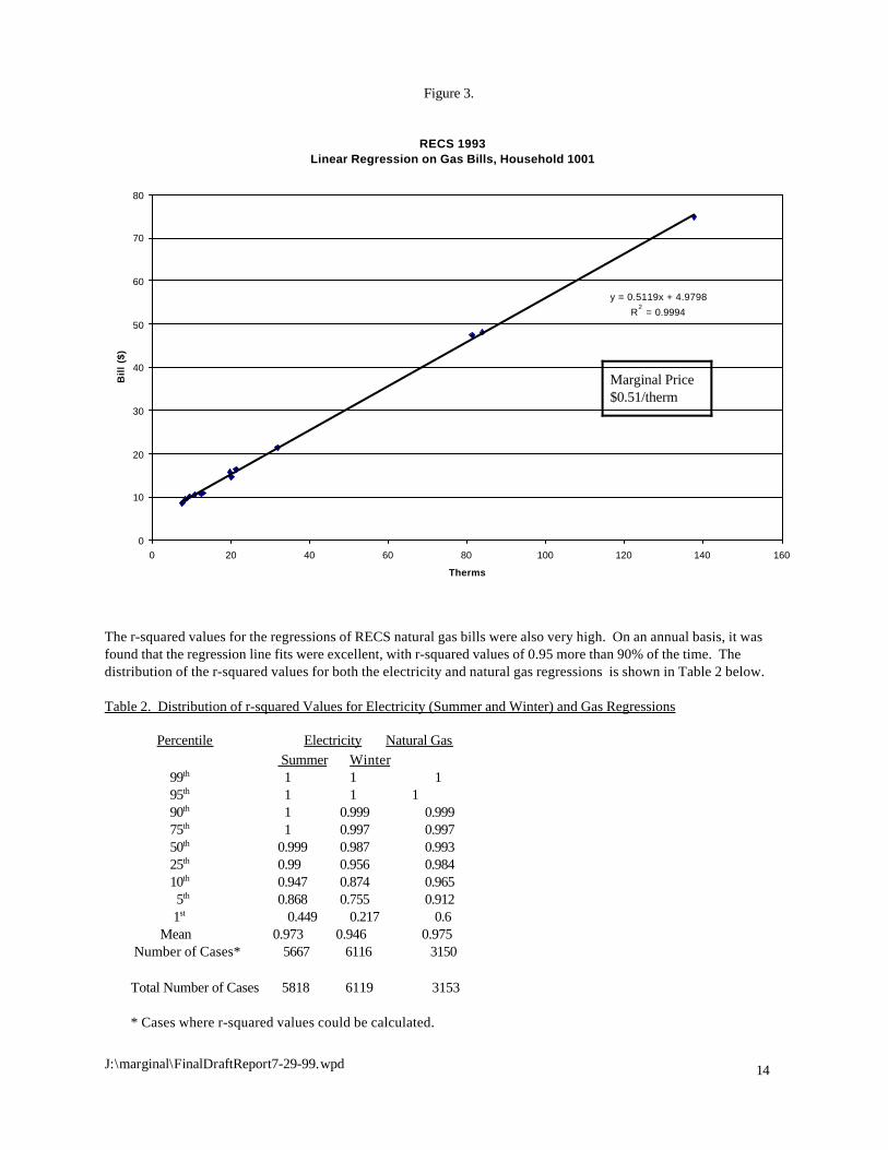
Natural GasFor natural gas, the data were not divided into seasons because review of gas utility rates (during the “Analytic”approach described earlier) found that most (21 out of 27) utilities surveyed did not have seasonal rates. Also, manyhouseholds have little or no gas consumption in the summer, making determination of a marginal price for this seasondifficult. Instead, a single regression relating natural gas bills and usage was performed using the data for all of thebilling cycles. It was possible to determine a slope of the regression line for all 3153 households for which billing datawere available. Slopes were rejected as unreasonable if they were less than or equal to zero, or greater than$3.20/therm. This left 3139 households, or 78% of the total of 4033 households that use natural gas. Again, most (880)of the households for which a marginal price was not available were those for which EIA did not collect billing data,with only 14 additional households dropped due to unacceptable regression slopes. See Figure 3 below for a samplelinear regression on the gas bills of one of the RECS households.
14J:\marginal\FinalDraftReport7-29-99.wpd
RECS 1993Linear Regression on Gas Bills, Household 1001
y = 0.5119x + 4.9798R
2 = 0.9994
0
10
20
30
40
50
60
70
80
0 20 40 60 80 100 120 140 160
Therms
Bil
l ($
)
Marginal Price$0.51/therm
Figure 3.
The r-squared values for the regressions of RECS natural gas bills were also very high. On an annual basis, it wasfound that the regression line fits were excellent, with r-squared values of 0.95 more than 90% of the time. Thedistribution of the r-squared values for both the electricity and natural gas regressions is shown in Table 2 below.
Table 2. Distribution of r-squared Values for Electricity (Summer and Winter) and Gas Regressions
Percentile Electricity Natural Gas Summer Winter
99th 1 1 1 95th 1 1 1 90th 1 0.999 0.999
75th 1 0.997 0.997 50th 0.999 0.987 0.993 25th 0.99 0.956 0.984
10th 0.947 0.874 0.965 5th 0.868 0.755 0.912
1st 0.449 0.217 0.6 Mean 0.973 0.946 0.975 Number of Cases* 5667 6116 3150
Total Number of Cases 5818 6119 3153
* Cases where r-squared values could be calculated.

15J:\marginal\FinalDraftReport7-29-99.wpd
Electricity and Natural GasA statistical analysis was performed comparing the data sets for each fuel before and after dropping the householdsfor which it was unable to calculate marginal energy prices in order to determine if any bias was being introduced bydropping those households. It was found that the subset of households that were dropped were those whose utilitybills were included in the household’s rent; presumably EIA could not collect billing data for those households.
Looking at just those subsets of RECS households that own the particular appliance of interest, it was found that thedifferences between all households and the subset for which it was able to calculate a marginal price were smaller thanthe differences described above for the set of all RECS households. These results may occur because householdswhich own clothes washers, or water heaters, or central air conditioners, tend to have a relatively lower proportion ofrenters in the first place, so fewer households of that type were dropped. For the key parameters, differences werefound to be negligible (generally 1% or less) between the appliance data set and the subset with marginal prices. Table 3 below shows the number and percent of households used in the analysis for each appliance subset afterhouseholds with no marginal price were dropped.
Table 3. Number of Households in Each Appliance Data Set, and in Subsets with Marginal Prices
Appliance Subsets
(HH = household)
All Households withappliance
Marginal Price Subset Marginal Price Subset aspercent of All Households
SurveyResponses
U.S.Households(millions)*
Survey
Responses
U.S.Households(millions)*
% ofSurveyResponses
% of RelevantU.S.Households
HHs with washer anddryer and electricity
4998 67.8 4574 61.9 92% 91%
HHs with washer anddryer and natural gas
2759 40.6 2439 35.6 88% 88%
HHs with central airconditioning
2414 32.1 2164 28.8 90% 90%
HHs with heat pumps 651 7.9 613 7.6 94% 96%HHs with electric waterheaters
2559 33.4 2323 30.3 91% 91%
HHs with natural gaswater heaters
2805 41.0 2535 36.0 90% 88%
HHs with fuel oil waterheaters**
176 1.8 163 1.7 93% 94%
* Sum of weights of households. The weight of each household is the number of US households represented by eachRECS household.
** “Marginal Price Subset” represents the households for which an electricity marginal price is available. Fuel oilmarginal price was assumed to be the same as the fuel oil average price, an assumption supported by the researchreported in Section V below.
Results of AnalysisFigures 4 and 5 below display the results of the residential electricity price analysis by showing the relationshipbetween marginal electricity prices and average electricity prices for the residential sector in the summer and thewinter. Figure 6 below displays the results (on an annual basis) of the residential gas analysis.
In the LCC analysis of three residential products (clothes washers, water heaters, and central air conditioners/heatpumps), the marginal electricity and natural gas prices used were derived directly from RECS. Figures 4, 5, and 6 belowshow how different these marginal prices are from average prices. Those marginal electricity prices in the summer(June-September) range from 98% below to 175% above the average price for the same customer. At the consumption-
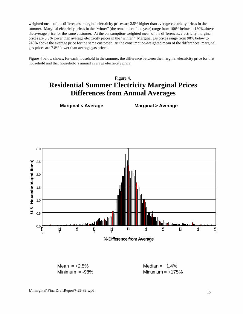
16J:\marginal\FinalDraftReport7-29-99.wpd
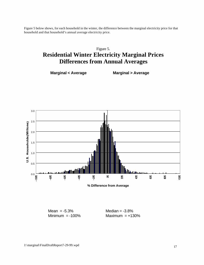
weighted mean of the differences, marginal electricity prices are 2.5% higher than average electricity prices in thesummer. Marginal electricity prices in the “winter” (the remainder of the year) range from 100% below to 130% abovethe average price for the same customer. At the consumption-weighted mean of the differences, electricity marginalprices are 5.3% lower than average electricity prices in the “winter.” Marginal gas prices range from 98% below to248% above the average price for the same customer. At the consumption-weighted mean of the differences, marginalgas prices are 7.8% lower than average gas prices.
Figure 4 below shows, for each household in the summer, the difference between the marginal electricity price for thathousehold and that household’s annual average electricity price.
Figure 4.
Residential Summer Electricity Marginal PricesDifferences from Annual Averages
0.0
0.5
1.0
1.5
2.0
2.5
3.0
% Difference from Average
Mean = +2.5% Median = +1.4%Minimum = -98% Minumum = +175%
Marginal > AverageMarginal < Average
17J:\marginal\FinalDraftReport7-29-99.wpd
Figure 5 below shows, for each household in the winter, the difference between the marginal electricity price for thathousehold and that household’s annual average electricity price.
Figure 5.
Residential Winter Electricity Marginal PricesDifferences from Annual Averages
0.0
0.5
1.0
1.5
2.0
2.5
3.0
% Difference from Average
Marginal > AverageMarginal < Average
Median = -3.8%Maximum = +130%
Mean = -5.3%Minimum = -100%
18J:\marginal\FinalDraftReport7-29-99.wpd
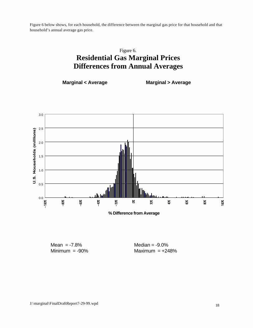
Figure 6 below shows, for each household, the difference between the marginal gas price for that household and thathousehold’s annual average gas price.
Figure 6.
Residential Gas Marginal PricesDifferences from Annual Averages
0.0
0.5
1.0
1.5
2.0
2.5
3.0
% Difference from Average
Marginal > AverageMarginal < Average
Mean = -7.8%Minimum = -90%
Median = -9.0%Maximum = +248%
19J:\marginal\FinalDraftReport7-29-99.wpd
Company Dixie Gas C&W Oil & Heating Powers Oil Co MacDuffie Petroleum Eastern PropaneLocation Verona VA Danbury CT Foxboro MA Hudson NH Rochester NHTerritory 3 counties in VA Fairfield County metro Attleboro MA NH, MA southern Maine
Price/gallon $0.85 $0.82 $0.75 $0.72 $0.66Discount cash paid in 5 days: $0.03 auto delivery: $0.03 paid in 7 bus days: $0.10 paid in 10 days: $0.10 none
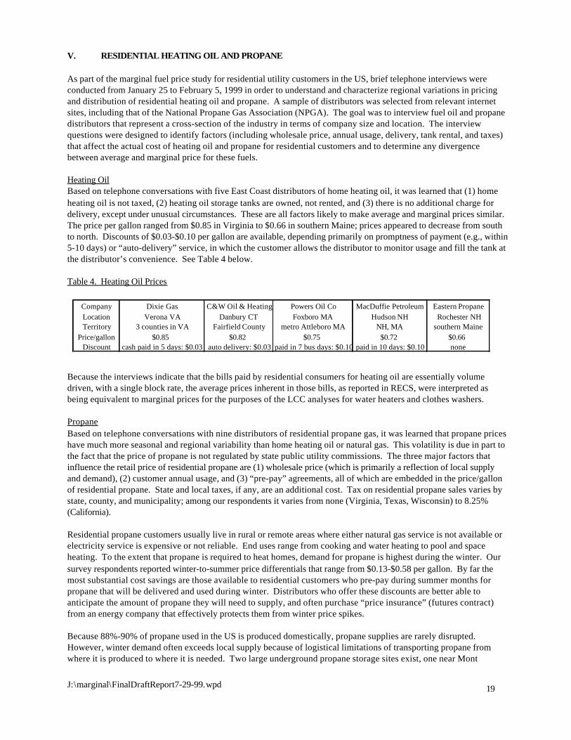
V. RESIDENTIAL HEATING OIL AND PROPANE
As part of the marginal fuel price study for residential utility customers in the US, brief telephone interviews wereconducted from January 25 to February 5, 1999 in order to understand and characterize regional variations in pricingand distribution of residential heating oil and propane. A sample of distributors was selected from relevant internetsites, including that of the National Propane Gas Association (NPGA). The goal was to interview fuel oil and propanedistributors that represent a cross-section of the industry in terms of company size and location. The interviewquestions were designed to identify factors (including wholesale price, annual usage, delivery, tank rental, and taxes)that affect the actual cost of heating oil and propane for residential customers and to determine any divergencebetween average and marginal price for these fuels.
Heating OilBased on telephone conversations with five East Coast distributors of home heating oil, it was learned that (1) homeheating oil is not taxed, (2) heating oil storage tanks are owned, not rented, and (3) there is no additional charge fordelivery, except under unusual circumstances. These are all factors likely to make average and marginal prices similar. The price per gallon ranged from $0.85 in Virginia to $0.66 in southern Maine; prices appeared to decrease from southto north. Discounts of $0.03-$0.10 per gallon are available, depending primarily on promptness of payment (e.g., within5-10 days) or “auto-delivery” service, in which the customer allows the distributor to monitor usage and fill the tank atthe distributor’s convenience. See Table 4 below.
Table 4. Heating Oil Prices
Because the interviews indicate that the bills paid by residential consumers for heating oil are essentially volumedriven, with a single block rate, the average prices inherent in those bills, as reported in RECS, were interpreted asbeing equivalent to marginal prices for the purposes of the LCC analyses for water heaters and clothes washers.
PropaneBased on telephone conversations with nine distributors of residential propane gas, it was learned that propane priceshave much more seasonal and regional variability than home heating oil or natural gas. This volatility is due in part tothe fact that the price of propane is not regulated by state public utility commissions. The three major factors thatinfluence the retail price of residential propane are (1) wholesale price (which is primarily a reflection of local supplyand demand), (2) customer annual usage, and (3) “pre-pay” agreements, all of which are embedded in the price/gallonof residential propane. State and local taxes, if any, are an additional cost. Tax on residential propane sales varies bystate, county, and municipality; among our respondents it varies from none (Virginia, Texas, Wisconsin) to 8.25%(California).
Residential propane customers usually live in rural or remote areas where either natural gas service is not available orelectricity service is expensive or not reliable. End uses range from cooking and water heating to pool and spaceheating. To the extent that propane is required to heat homes, demand for propane is highest during the winter. Oursurvey respondents reported winter-to-summer price differentials that range from $0.13-$0.58 per gallon. By far themost substantial cost savings are those available to residential customers who pre-pay during summer months forpropane that will be delivered and used during winter. Distributors who offer these discounts are better able toanticipate the amount of propane they will need to supply, and often purchase “price insurance” (futures contract)from an energy company that effectively protects them from winter price spikes.
Because 88%-90% of propane used in the US is produced domestically, propane supplies are rarely disrupted. However, winter demand often exceeds local supply because of logistical limitations of transporting propane fromwhere it is produced to where it is needed. Two large underground propane storage sites exist, one near Mont

20J:\marginal\FinalDraftReport7-29-99.wpd
Bellvue, Texas, and the second outside of Conway, Kansas. Three pipelines transport propane from these reservoirsto southern, eastern, and midwestern states. Bulk storage facilities are located at regional hubs along each pipeline;trucks transport propane between these hubs and regional distributors, who distribute the fuel to residentialcustomers. Two of the three pipelines also carry other petroleum products, so propane delivery is often interrupted.
The cost of distributing propane (from the refinery or port to a bulk storage facility) and delivering it to the residentialcustomer is incorporated in the price per gallon that each customer is charged. The lowest price per gallon ($0.65) wasreported in northern Wisconsin, while the highest price ($1.41) was reported in Galveston, near Mont Bellvue, Texas,and adjacent to several refineries. One possible explanation for this apparent anomaly is that the price of propane inWisconsin (where winters are harsh) is driven down by high demand and fierce competition, while the price in coastalTexas (where winters are mild) is buoyed up by relatively low demand and little competition. In fact, our resultssuggest that local competition (which increases along with local demand) is more a determinant of the wholesale pricethan is the distance from the propane source.
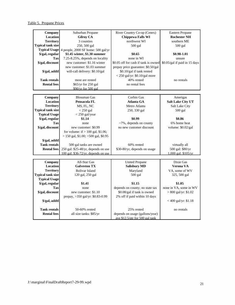
Next to local wholesale price, total annual usage has the largest effect on residential propane prices. The price pergallon reported in Table 5 below represents the retail price to a customer who uses a typical amount of propanecompared to residential customers in that particular service territory. Volume discounts are usually available to thosewho use more than the typical amount of propane; volume discounts reported by our contacts range from $0.02/gal(Utah) to $0.19/gal (Florida). Similarly, customers who use less than the typical amount of propane pay more than theregular price per gallon; distributors reported additional costs of $0.10 (Wisconsin) to $0.13 (Virginia). Propanedistributors often offer discounts to new residential customers because (1) they want new customers and (2) it takes ayear to determine the usage of each new customer. Contacts reported new customer discounts of none (Georgia) to$0.15 (Florida) to $0.31 (Texas).
Residential customers store propane in on-site tanks that range in size from 100 to 1,000 gallons; tank size increaseswith the number of end uses, severity of the climate, and difficulty of site access. Some customers lease (rent) tanksfrom their propane distributor. Renting relieves the customer of responsibility for tank maintenance and providesflexibility for temporary or mobile home owners, but prevents the customer from shopping around for the lowest fuelprice among local distributors. Customers who purchase their own tanks do so for several reasons. Permanent, year-round homes in rural areas tend to have a larger number of propane end uses and bigger tanks, which, because theyare unsightly and take up space, tend to be installed underground. Distributors are reluctant to lease undergroundtanks because leak detection and maintenance is more difficult, so buried tanks are usually owned. Owning a storagetank also allows a customer to shop around for the best available propane price. Among our respondents, percentageof tanks leased from a distributor ranges from none (Maine, Virginia) to virtually all (Utah, California). Tank rental feesdepend on tank size and/or annual usage; annual fees range from none (Wisconsin) to $100 (Utah), but generally theyare $50-100.
Because the interviews with propane distributors indicate that the bills paid by residential consumers for propane areessentially volume driven, with a single block rate, the average prices inherent in those bills, as reported in RECS, wereinterpreted as being equivalent to marginal prices for the purposes of the LCC analyses for water heaters and clotheswashers.
21J:\marginal\FinalDraftReport7-29-99.wpd
Company Suburban Propane River Country Co-op (Cenex) Eastern PropaneLocation Gilroy CA Chippewa Falls WI Rochester NHTerritory 3 counties northwest WI southern ME
Typical tank size 250, 500 gal 500 gal 500 galTypical Usage 4 people, 2000 SF home: 500 gal/yr$/gal, regular $1.45 winter, $1.30 summer $0.65 $0.98-1.01
Tax 7.25-8.25%, depends on locality none in WI unsure$/gal, discount new customer: $1.16 winter $0.05 off for cash if tank is owned $0.05/gal if paid in 15 days
new customer: $1.03 summer prepay price guarantee: $0.50/gal$/gal, addtl will-call delivery: $0.10/gal $0.10/gal if tank rented
< 250 gal/yr: $0.10/gal moreTank rentals most are rented 40% rented no rentals
Rental fees $65/yr for 250 gal no rental fees$90/yr for 500 gal
Company Blossman Gas Corbin Gas AmerigasLocation Pensacola FL Atlanta GA Salt Lake City UTTerritory MS, FL, NC Metro Atlanta Salt Lake City
Typical tank size < 250 gal 250, 330 gal 500 galTypical Usage < 250 gal/year$/gal, regular $1.14 $0.99 $0.86
Tax none ~7%, depends on county 6% home heat$/gal, discount new customer: $0.99 no new customer discount volume: $0.02/gal
for volume: if > 100 gal. $1.06;> 150 gal, $1.00; >500 gal, $0.95
$/gal, addtlTank rentals 500 gal tanks are owned 60% rented virtually all
Rental fees 250 gal: $25-48/yr, depends on use $30-80/yr, depends on usage 500 gal: $80/yr100 gal: $36-72/yr, depends on use 1,000 gal: $105/yr
Company All-Star Gas United Propane Dixie GasLocation Galveston TX Salisbury MD Verona VATerritory Bolivar Island Maryland VA, some of WV
Typical tank size 120 gal, 250 gal 500 gal 325, 500 galTypical Usage$/gal, regular $1.41 $1.15 $1.05
Tax none depends on county; no state tax none in VA, some in WV$/gal, discount new customer: $1.10 $0.08/gal if tank is owned > 800 gal/yr: $1.02
prepay, >350 gal/yr: $0.83-0.99 2% off if paid within 10 days$/gal, addtl < 400 gal/yr: $1.18
Tank rentals 50-60% rented 25% rented no rentalsRental fees all size tanks: $85/yr depends on usage (gallons/year)
ave $12.5/qtr for 500 gal tank
Table 5. Propane Prices

9 The highest single tax rate for energy that the research uncovered was for one small city in California that imposes autility users tax of 9.9%. Otherwise, the highest utility users tax rate the research uncovered is 8%. State-level salestaxes and other state-level taxes can raise the effective tax to consumers beyond these levels, though. 10 EIA, “End Use Taxes: Current EIA Practices,” August 1994, page 29.
22J:\marginal\FinalDraftReport7-29-99.wpd
VI. TAXES
OverviewThe marginal energy prices that consumers experience can be affected by the taxes that those consumers pay as partof their energy bills. Those energy bills can include taxes in two fundamentally different ways. First, tax obligationsthat an energy utility itself incurs (such as federal income taxes and property taxes) are most often considered to bepart of the utility’s revenue requirements. Consequently, such taxes are embedded within approved utility rates; theyare not itemized on utility bills (even the unbundled bills that are becoming more prevalent in the utility industry,particularly as electricity restructuring occurs in more states). Prices paid by consumers are higher (than theyotherwise would be) to the degree that these sorts of taxes are included in their utilities’ base rates. But, becauseconsumer energy savings (from using appliances that are more energy efficient) would not directly and immediatelyreduce the level of these embedded taxes, the existence of these taxes does not affect the calculation of consumers’marginal energy prices in a manner that is relevant to this research project.
The second, and more directly visible, way in which consumers pay taxes when they pay their energy bills is throughpaying various sorts of taxes (or fees) as direct add-ons to their energy bills. These taxes (such as utility users taxes,franchise fees, and regulatory fees) are often called “pass-through” taxes. They are taxes assessed by state and/orlocal jurisdictions. They are collected by utilities on behalf of consumers and then are passed on by those utilities tothe jurisdictions that imposed them. Since these taxes are not considered to be part of a utility’s revenuerequirements, they are not embedded within utility rates. Rather, such taxes are listed as line items on consumers’bills. The marginal prices that consumers pay for energy are directly affected by the existence of this type of tax;indeed, consumers’ marginal energy prices are higher than they would be if these taxes and fees did not exist. Thistype of tax is usually assessed as either a fixed percentage of the pre-tax energy bill or as a fixed dollar amount perenergy unit. In some instances, pass-through taxes using both types of assessment mechanisms are added toconsumers’ bills. For either type of pass-through tax assessment, the consumption of less energy (due to usingappliances that are more energy-efficient) will reduce (on a direct and immediate basis) the tax portion of the energy billas well as the non-tax portion of that bill. For that reason, this research project is interested in the degree of thosesavings.
Range and Magnitude of Pass-Through TaxesBecause pass-through taxes are assessed by individual states and local jurisdictions, they can vary widely in theirmagnitude, even within the same utility service territory (see below). There are four main types of pass-through taxes:
1) state sales taxes (see Appendix 5, Table 6)2) state utility regulatory assessments (see Appendix 5, Table 7)3) state taxes on units of energy (see Appendix 5, Table 8)4) local utility users taxes
These taxes individually range in size from being non-existent in some areas to being as much as 10% in other areas9. In addition, because these sorts of taxes are set by various government agencies, they rarely appear on publishedutility tariffs. They appear as line item charges on consumers’ actual bills. Therefore, determining what these taxes(especially those that are locally imposed) really are for particular customers of particular utilities would be a verydifficult task. As EIA said in its 1994 report “End-Use Taxes: Current EIA Practices,”
“Adding statutory taxes to pre-tax prices is a tedious, error-prone process. … Because of the widevariety of taxes imposed by local governments, the tax adjustment is only practicable at the State level.”10

11 Ibid, Table B2. The relevant portions of EIA’s Table B2 are shown in Appendix 5, Table 6 of this report.12 The Alliance to Save Energy, “State and Local Taxation: Energy Policy by Accident,” 1994.13 For example, in the Pacific Gas and Electric Company (PG&E) service territory of northern California, the size of thepercentage-based utility users tax, which is applied to both the electricity and natural gas components of a PG&Ecustomer’s bill, varies from 0% in many of the cities and counties served by PG&E to as much as 9.9% in one city,8.0% in five cities and 7.5% in eight cities. A total of 68 cities in PG&E’s service area currently impose this type of taxon energy consumption by their residents. While higher utility users tax rates may exist in California or in other states,no evidence of them was found.14 Andrew Hoerner, Center for a Sustainable Economy, personal communication, February 10, 1999. Additionalsources whose web sites were consulted for information on state and local energy taxes included The Federation ofTax Administrators, EPRI, and The Multistate Tax Commission.
23J:\marginal\FinalDraftReport7-29-99.wpd
The EIA report provides a state-by-state list of sales and use taxes on end-use energy consumption.11 It also indicatesthe states in which energy consumption (by energy fuel type) is exempt from state sales and use taxes. In addition,this report includes an estimate of the magnitude of the possible effect of including State sales taxes in energy prices. For electricity prices, EIA’s report shows that on average electricity prices for the residential sector rise only 0.9% withthe inclusion of state sales taxes. The range of increase in individual states is from 2% to 6.5% for those states whereelectricity consumption in the residential sector is not exempt from sales tax. For the commercial sector, the rise inelectricity prices due to the inclusion of the applicable state sales taxes would be 4.2% on average for the nation, witha range by state of from 3% to 8% for those states where electricity consumption is not exempt from sales tax. (EIA’sreport does not include similar estimates of the effect of including state sales taxes on the consumption of natural gas.)
To get a sense for the magnitude and variation of other state and local-level taxes, various sources were consulted. The most comprehensive survey of other taxes on a state level was found in a report on state and local taxation by theAlliance to Save Energy (ASE).12 This report reveals that percentage taxes for regulatory assessments in the 39 statesthat impose them (see Appendix 5, Table 7; taken from ASE’s report) range in size from 0.02% to 0.50%. In otherstates, such as California, cities can charge consumers a utility users tax. One city imposes a 9.9% utility users tax.13 Several other cities set this tax as high as 7.5% or 8.0%.
Taxes or fees on units of energy consumed range in size from 0.015 cents per kWh to 0.26 cents per kWh in the ninestates (see Appendix 5, Table 8; taken from ASE’s report) that impose that type of tax on energy used by consumers. In California, for instance, while PG&E customers pay a $0.0002/kWh in support of the California Energy Commission,customers of SDG&E also pay regulatory fees amounting to $0.00012/kWh on the electricity portion of their bills and$0.00078/therm on the gas portion of their bills. States that have no sales taxes are not prohibited from imposingelectric and gas regulatory assessments and kWh taxes on electricity. Variations and anomalies such as these make anexhaustive study of the actual taxes and fees associated with utility energy bills around the country, and even thoseassociated with this project’s modest utility sample, beyond our scope. Indeed, it is unlikely that anyone has everconducted a survey of state and local taxes comprehensive enough to capture the type of utility users taxes that canoccur in California alone.14 As a result, the effect of taxes on marginal prices was addressed in the manner outlinedbelow.
Impact of Taxes on Marginal PricesPass-through taxes increase consumers’ energy bills; they also increase consumers’ marginal prices. For apercentage-based pass-through tax (like the utility users tax described above), which is applied to the whole energybill (including any fixed charges, such as customer charges), the consumer’s marginal price is increased by thepercentage size of the tax itself. Thus, an 8% tax would increase a consumer’s marginal price by 8%. Consumers taxedat the 2% level would have a marginal price 2% higher than if they paid no pass-through taxes. Because taxes on unitsof energy (like the per kWh regulatory fees described above) do not apply to fixed charges, they raise marginal pricesin a non-linear, but still minor and easily calculated, manner.
Impact of Taxes on SavingsSince consumers both pay and save at a rate equal to the marginal price, other things being equal, reductions inenergy consumption due to new appliance energy efficiency standards will cause reductions in the size of the pass-through

15 EIA, “Energy Sales and Revenue 1997,” page 1.
24J:\marginal\FinalDraftReport7-29-99.wpd
taxes consumers pay, whether those taxes are percentage taxes or per-unit taxes. The resulting reductions in taxpayments are savings to the consumer directly associated with the more efficient appliances. Consumers facing 8%tax prices will save an additional 8% beyond what they would have saved if they did not have to pay such taxes in thefirst place. Consumers with 2% taxes will save an additional 2% of their (pre-tax) bill when their energy consumption isreduced by using appliances that are more energy-efficient.
Treatment of Taxes in This Research ProjectThis project used two main approaches to derive marginal prices. The RECS-based approach used actual consumerbills that already include all taxes (both those embedded in utility rates and pass-through taxes). Therefore, themarginal prices derived from those bills “automatically” take into account the effects of changes in taxes due tochanges in energy consumption. For use in life-cycle cost or savings analyses, no further adjustments are needed toreflect the existence of taxes in the marginal prices derived from the RECS-based approach.
The MAISY®-based approach involved using distributions of both building energy usage levels (from the MAISY®
database) and utility tariffs to derive commercial electricity bills. Because those utility tariffs do not already includepass-through taxes, the marginal prices derived by this approach are smaller than they otherwise would be to thedegree that pass-through taxes apply to the sampled buildings. Therefore, when analyzing the results of this researcheffort, consideration should be given to the applicability of the four types of pass-through taxes mentioned here(state-level sales and use taxes, other state-level % taxes, $ per energy unit taxes, and locally imposed utility userstaxes) to derive marginal electricity prices for commercial buildings that include taxes. While adding the pass-throughtaxes applicable at the state level (from the EIA and ASE report tables shown below) would involve a non-trivial andvery time-consuming, but still relatively straightforward exercise, there is no clear way to obtain the level of the locallydetermined utility users tax that might apply to the sampled buildings. Therefore, because of the lack ofcomprehensive information on the magnitude of the locally imposed utility users taxes, one must be aware that themarginal prices so calculated may not be as high as they really should be wherever those taxes would apply. Thus,marginal prices and savings for an individual consumer may still be understated by from 0% to 10%.
Taxes and Average PricesOnce marginal prices are calculated and taxes are considered, a comparison with regularly published average prices,such as those issued by EIA, may be desired. Those published average prices are calculated by dividing utilityrevenues by sales. With regard to whether or not these published average prices include taxes, the underlyingquestion is which taxes are included in utility revenues. It is clear that embedded taxes are included within the utilityrevenue requirements that form the basis for utility revenues through the traditional rate-setting process; however, it isnot clear whether pass-through taxes are considered to be part of utility revenues. In response to the request forclarity on this issue, EIA referred us to a page in EIA’s “Electric Sales and Revenue 1997” report that contains thefollowing statement:
“Taxing authorities differ on whether a specific tax is assessed to the utility or to the consumer, a differencethat in turn determines whether or not the tax is included in the electric utility’s operating revenues.”15
Therefore, it is concluded that one cannot know for sure whether pass-through taxes, especially those imposed bylocal government agencies, are included in utility revenues and thus included in average prices. While this lack ofcertainty about the inclusion of pass-through taxes in published average prices jeopardizes any comparison ofaverage and marginal prices, it is believed that comparing RECS-based marginal prices with published average priceswould be more sound, for example, than comparing marginal prices derived by the MAISY®-based approach (wheretaxes must be added in manually) with published average prices.
Tax Feedback LoopsSome might argue that local governments (and perhaps even state governments) might raise their locally-imposedutility tax rates if the revenues they obtain from consumers’ energy bills decline because consumers use less energy asa consequence of improved appliance energy-efficiency standards. This project did not attempt to analyze such

25J:\marginal\FinalDraftReport7-29-99.wpd
positions. It is noted that while similar arguments have been made during debates on electric industry restructuringoccurring around the country, there is no widespread agreement on their validity.
ConclusionThis report has not attempted to account for all appropriate taxes in the calculation of marginal energy prices in theanalysis because it is essentially impossible to do so. Comparisons between published average energy prices andcalculated marginal energy prices must be made with care because they are subject to error for the same reasons. Thisreport indicates the degree of error that may be present.
The derivation of commercial consumer marginal electricity prices excludes pass-through taxes and thusunderestimates consumers’ marginal bill savings by 0% to as much as 10%, depending upon the level of state andlocally imposed taxes. In contrast, the derivation of marginal electricity and gas prices for the residential sector fromactual consumer bills from RECS includes pass-through taxes; thus, the underestimation of consumers’ marginal billsavings inherent in the commercial analysis does not exist in the residential analysis.

26J:\marginal\FinalDraftReport7-29-99.wpd
Appendix 1. Tariffs Used in the Commercial Analysis
Utility State Tariff Utility State Tariff
Alabama PowerAlabama PowerAlabama PowerAppalachian Power CoArizona Public ServiceArizona Public ServiceBoston EdisonBoston EdisonCentral Power and LightCleveland Electric Illum. CoCleveland Electric Illum. CoCommonwealth Edison CoDetroit EdisonJersey Central Power & LightMadison G&EMadison G&ENSPNSPNSPNSP
A LA LA LVAA ZA ZMAMATXOHOHILMINJW IW IMNMNW IW I
LPEMLPMLPSSGSE30E32G-1 G-221Gen CommLg CommRate 6 non-TOUD3GSCg-1Cg-5A10, D12, E13A14, D16,E15Cg-2Cg-2 unmetered
NSPNiagara Mohawk Power CorpNiagara Mohawk Power CorpOhio Power CompanyPEPCOPacific Gas and ElectricPacific Gas and ElectricPennsylvania Power & LightPennsylvania Power & LightPoudre ValleySavannah Electric and PowerSeattle City LightSeattle City LightSoCal EdisonSoCal EdisonUnion Electric Co.Union Electric Co.Virginia Power CompanyWisconsin Electric Power
W INYNYOHDCCACAPAPACOGAW AW ACACAMOMOVAW I
Cg-5SC-2 DemandSC-2 Non-DemandGS3-11GSA1A10GS-1GS-3B-97GS-7Rate 31Rate 34GS-1GS-2No. 2No. 3GS-1Cg 1

27J:\marginal\FinalDraftReport7-29-99.wpd
Appendix 2. Examples of Commercial Bill Calculations
Commercial tariffs generally fall into two categories, non-demand and demand. Demand is measured in kilowatts (kW)required by the customer over a relatively short time period, often 30 minutes. Meters are installed at the customer siteto measure monthly and sometimes annual peak demand, and these are used to compute the demand component of thecustomer’s bill.
Typically demand tariffs are assigned to large customers, such as office buildings, hospitals, and malls. Non-demandtariffs are assigned to smaller customers, such as restaurants and small grocery stores. An example of each isillustrated below.
Example 1: Non-demand tariff
Utility: Alabama PowerTariff: Commercial, LPSCustomer Base Charge: $8.65/mo.Summer Energy Charge: $0.06223/kWhWinter Energy Charge: $0.05843/kWh
Customer: Usage: 2547 kWhMonth: JanuaryBaseline Bill: $157.47 = 8.65 + ($0.05843 * 2547)
Bill with 5% Usage Decrement: (Figures below include rounding)Usage: 2420 kWh = 2547 kWh – (0.05 * 2547 kWh)Bill: $150.03 = 8.65 + ($0.05843 * 2420)
Monthly Average Price: $0.06183/kWh = $157.47 / 2547Monthly Marginal Price: $0.05843/kWh = Bill Savings / Energy Savings
= ($157.47 - $150.03) / (2547 - 2420)
Example 2: Demand Tariff
Utility: Southern California EdisonTariff: Commercial GS2Tariff Min/Max kW: 80 - 2000 kW/hr (measured over 15 minutes)Customer Base Charge: $60.30/mo.Energy Block Cutoffs: Block 1: 300 kWh/kW (based on monthly peak kW)Energy Charge, Block 1: $0.07692/kWhEnergy Charge, Block 2: $0.04391/kWhDemand Charge Component 1: $5.40 (Summer), $5.40 (Winter)Demand Charge Component 2: $7.75 (Summer), $0.00 (Winter)
Customer Usage: 150388 kWhMonth: May
Monthly Peak kW: 71 kW (over 15 minutes)Baseline Bill: $7750.35 = $60.30 + ((300*71)*$0.07692) + ((150388 - (300*71))*$0.04391)
+ (71*$5.40)Bill with 5% Energy and4% Demand Decrement: $7376.71 = $60.30 + ((300*(71*0.96))*$0.07692)
+ (((150388*0.95) - (300*(71*0.96)))*$0.04391) + ((71*0.96)*$5.40)
Monthly Average Price: $0.05163/kWh = 7376.71 / (150388*0.95)Monthly Marginal Price: $0.04969/kWh = Bill Savings / Energy Savings
= ($7750.35 - $7376.71) / (150388 - (150388 * 0.95))

16 See comment #12 on the Draft Report on Potential Impact of Possible Energy Efficiency Levels for Fluorescent LampBallasts,, received by DOE from Steve Rosenstock of EEI on August 28, 1997.
28J:\marginal\FinalDraftReport7-29-99.wpd
Appendix 3. Demand Decrement Due to Standards - The Role of Lighting Coincidence and Diversity
In the process of marginal price estimation, it is necessary to account for demand charges in the calculation of somecommercial sector bills. Demand charges depend upon the peak building demand (kW) each month. For eachcustomer or building analyzed, the monthly energy use (kWh) and the monthly demand (kW) are based on actualannual kWh and actual summer and winter peak kW and summer and winter average peak kW. Since a change fromenergy-efficient magnetic (EEM) ballasts meeting the current standard to electronic ballasts for four-foot T12 systemswould save about 15% of lighting energy used by fluorescent lamps and since about 30-35% of building energy use isfor lighting, about 5% of building energy use will be saved if EEM ballasts are converted to electronic ballasts. The5% reduction was assumed to occur every month.
It is also necessary to estimate the reduction in peak demand if building energy use is reduced by 5% on average. Some analysts prefer to discuss this issue in terms of diversity and coincidence. Coincidence is the lighting kW duringthe building peak divided by the lighting peak kW. In this situation, the coincidence factor was expected to be closeto 1.0 since, whatever the maximum number of lamps that operate during the lighting peak, a very similar number oflamps can be expected to operate during the building peak. EEI has suggested using 0.9 for the default coincidencefactor.16
Coincidence factor (C) = lighting kW during building peak/lighting peak kW
The diversity factor is a measure of the percent of the installed kW for lighting used during the lighting peak. Diversity is already accounted for because the actual building energy usage (which comes from the MAISY®
database) already excludes those lamps not in use during some parts of the day. Instead the concern is with lightingaverage kW because that is, in essence, reduced by 5% in the bill calculator when monthly energy use is reduced by5%. It is assumed that the lighting hours do not change when more efficient ballasts are installed.
Diversity (D) = lighting peak kW/lighting kW installed
Some analysts might multiply coincidence (C) times diversity (D); that would not yield the desired ratio of lighting kWduring the building peak to lighting average kW.
In relative terms, demand reduction is assumed to be 80% of energy savings. For 5% energy savings, it is assumedthat the demand reduction would be 4% of peak kW. This means that if 500 identical fixtures are operating on average,that only 400 (or 80%) are operating during the building peak demand period. The 80% value relative to the averagevalue is used because the monthly lighting energy use can be considered to be equal to some average kW times themonthly lighting hours and the monthly lighting energy use is reduced by a fixed percentage.

29J:\marginal\FinalDraftReport7-29-99.wpd
Appendix 4: Weighting Method for Commercial Sample
The composition of the commercial sample posed a dual weighting problem: distributing weights across buildings andacross the approximately 20 tariffs that were applied to each building. The weighting approach solves these problemssequentially. The first step is to develop building weights, derived from the original MAISY® building weight andscaling factors (based on kWh usage), as discussed below. This adjusted building weight is then apportioned acrossall the tariffs (weighted by annual MWh sales) that were applied to the building. The composite weighting factor foreach building/tariff pair combines both of these weighting factors.
Calculation of Adjusted Building WeightsEach building in the sample is viewed as representing a share of the commercial buildings in its region of the US. Stateand regional scaling factors were developed and used to rescale the individual buildings’ MAISY® weights torepresent national usage, as described below.
The first step was to account for the fact that the sample was a subset of the MAISY® buildings for each state. Foreach of the seven states a state factor was computed:
state in the buildings sampledfor weightsMAISY of Sum
state in the buildings allfor weightsMAISY of Sum Factor State
=
The statewide energy usage represented by each sampled building was then computed by multiplying the building’sMAISY® weight by its average annual energy usage and the state factor. For each sampled building i:
Building i’s Adjusted State Energy Use = Annual kWh i * MAISY® Weight i * State Factor
The next step was to scale state usage to regional usage. US Census Divisions were assigned to one of seven regions, each represented by a state in our sample. Census Divisions not directly represented by a state in oursample were assigned to a state representing the most similar adjacent division. The table below shows the mappingof sampled states to Census Divisions.
Assignment of Sampled States to Census Divisions for Weighting Calculations
Sampled State Census Division(s) RepresentedNew York Middle Atlantic, New EnglandIllinois East North Central, West North CentralGeorgia South Atlantic, East South CentralTexas West South CentralColorado MountainWashington Pacific Contiguous (excluding California), Pacific Noncontiguous California California
Region Factors were then computed based on state and regional commercial retail electricity sales derived from 1998EIA data (see the table below). The Region Factors are the ratio of commercial sector electricity sales in the division(s)corresponding with each of the sampled states to the commercial sector electricity sales in each of those individualstates.
Sales Commercial Retail State
Sales Commercial Retail RegionalFactorRegion =
Applying the Region Factors was the next step in computing the Adjusted Building Weights for each building:
Building i’s Adjusted Region Energy Use = Region Factor * Building i’s Adjusted State Energy Use

17 The annual reports that IOUs submit to FERC, “Form 1 - Annual Report for Major Electric Utilities, Licensees, andOthers”, include information on the utilities’ sales, number of customers, and average rate by tariff or rate schedule on“page” 304 of that form (“Sales of Electricity by Rate Schedules”). An electronic database of the FERC Form 1 filings(that included page 304 data) was obtained from a commercial service known as Energy Central News.
30J:\marginal\FinalDraftReport7-29-99.wpd
Derivation of State and Regional Weights Used in Computed Tariff Average RatesSum of Bldg Wts Commercial kWh (millions)
StateSampled Buildings State
State Factor State Region
Region Factor
California 24506 557548 22.75 6710 6710 1.00Colorado 12698 84339 6.64 1203 4933 4.10Georgia 14022 140103 9.99 2369 20465 8.64Illinois 15645 205813 13.16 4312 17431 4.04New York 28734 331675 11.54 3895 12526 3.22Texas 46881 331176 7.06 6142 8911 1.45Washington 18221 120664 6.62 1833 3306 1.80
Total 160707 1771318 74282
The final step in calculating the Adjusted Building Weight takes each building as a share of the national total. Foreach sampled building i:
buildings sampled allfor Energy UseRegion Adjusted of Sum
Energy UseRegion Adjusted WeightBuilding Adjusted i
i =
For each sampled building, the Adjusted Building Weight is the percentage of national energy use represented by thatbuilding.
Derivation of Weights for Building/Tariff PairsIn the second phase of the weighting process, the weight for each building was apportioned across the applicabletariffs that had been used to compute marginal prices for it. These building/tariff weights sum to one for the entiresample and to the Adjusted Building Weight for each sampled building.
A different set of weights was computed for each sampled building because a unique set of tariffs was applied to eachsampled building based on its particular pattern of energy usage. The building-specific tariff weights were computedusing the FERC data on MWh sales for each tariff.17
This process was implemented in two steps.
The first step was to calculate the relative weight of each of the tariffs that were applied to a building. For eachbuilding (denoted by i) and tariff (denoted by j):
i Building toApplicable Tariffs Allfor SalesMWh of Sumj Tarifffor SalesMWh
i Buildingfor j Tariff of Share =

31J:\marginal\FinalDraftReport7-29-99.wpd
The building-specific tariff weights were then combined with the adjusted building weights to obtain a unique weightfor each building/tariff pair:
Weight for Building i on Tariff j = Adjusted Building Weight i * Share of Tariff j for Building i
These are the weights that were used to calculate weighted averages for the sample and for binning the data to derivethe distribution of percent differences between average and marginal prices (called epsilons) for use in the LCCanalysis.
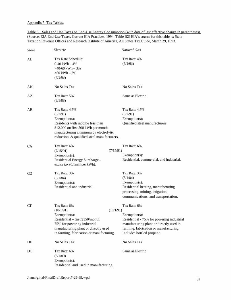
32J:\marginal\FinalDraftReport7-29-99.wpd
Appendix 5. Tax Tables.
Table 6. Sales and Use Taxes on End-Use Energy Consumption (with date of last effective change in parentheses) (Source: EIA End-Use Taxes, Current EIA Practices, 1994. Table B2) EIA’s source for this table is: StateTaxation/Revenue Offices and Research Institute of America, All States Tax Guide, March 29, 1993.
State Electric Natural Gas
AL Tax Rate Schedule: Tax Rate: 4%0-40 kWh – 4% (7/1/63)>40-60 kWh – 3%>60 kWh – 2%(7/1/63)
AK No Sales Tax No Sales Tax
AZ Tax Rate: 5% Same as Electric(6/1/83)
AR Tax Rate: 4.5% Tax Rate: 4.5%(5/7/91) (5/7/91)Exemption(s): Exemption(s):Residents with income less than Qualified steel manufacturers.$12,000 on first 500 kWh per month,manufacturing aluminum by electrolyticreduction, & qualified steel manufacturers.
CA Tax Rate: 6% Tax Rate: 6%(7/15/91) (7/15/91)Exemption(s): Exemption(s):Residential Energy Surcharge-- Residential, commercial, and industrial.excise tax (0.1mill per kWh).
CO Tax Rate: 3% Tax Rate: 3%(8/1/84) (8/1/84)Exemption(s): Exemption(s):Residential and industrial. Residential heating, manufacturing
processing, mining, irrigation,communications, and transportation.
CT Tax Rate: 6% Tax Rate: 6%(10/1/91) (10/1/91)Exemption(s): Exemption(s):Residential – first $150/month; Residential - 75% for powering industrial75% for powering industrial manufacturing plant or directly used inmanufacturing plant or directly used farming, fabrication or manufacturing.in farming, fabrication or manufacturing. Includes bottled propane.
DE No Sales Tax No Sales Tax
DC Tax Rate: 6% Same as Electric(6/1/80)Exemption(s):Residential and used in manufacturing.
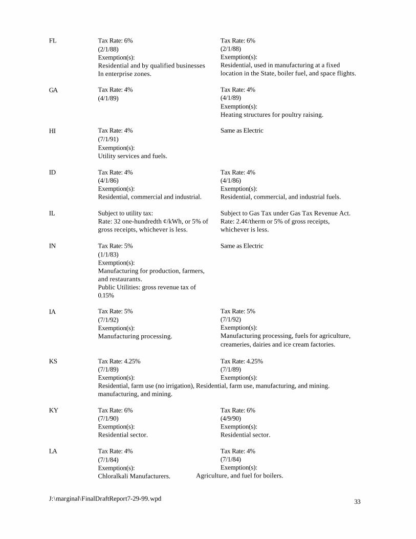
33J:\marginal\FinalDraftReport7-29-99.wpd
FL Tax Rate: 6% Tax Rate: 6%(2/1/88) (2/1/88)Exemption(s): Exemption(s):Residential and by qualified businesses Residential, used in manufacturing at a fixedIn enterprise zones. location in the State, boiler fuel, and space flights.
GA Tax Rate: 4% Tax Rate: 4%(4/1/89) (4/1/89)
Exemption(s):Heating structures for poultry raising.
HI Tax Rate: 4% Same as Electric(7/1/91)Exemption(s):Utility services and fuels.
ID Tax Rate: 4% Tax Rate: 4%(4/1/86) (4/1/86)Exemption(s): Exemption(s):Residential, commercial and industrial. Residential, commercial, and industrial fuels.
IL Subject to utility tax: Subject to Gas Tax under Gas Tax Revenue Act.Rate: 32 one-hundredth ¢/kWh, or 5% of Rate: 2.4¢/therm or 5% of gross receipts, gross receipts, whichever is less. whichever is less.
IN Tax Rate: 5% Same as Electric(1/1/83)Exemption(s):Manufacturing for production, farmers,and restaurants.Public Utilities: gross revenue tax of0.15%
IA Tax Rate: 5% Tax Rate: 5%(7/1/92) (7/1/92)Exemption(s): Exemption(s):Manufacturing processing. Manufacturing processing, fuels for agriculture,
creameries, dairies and ice cream factories.
KS Tax Rate: 4.25% Tax Rate: 4.25%(7/1/89) (7/1/89)Exemption(s): Exemption(s):Residential, farm use (no irrigation), Residential, farm use, manufacturing, and mining.manufacturing, and mining.
KY Tax Rate: 6% Tax Rate: 6%(7/1/90) (4/9/90)Exemption(s): Exemption(s):Residential sector. Residential sector.
LA Tax Rate: 4% Tax Rate: 4%(7/1/84) (7/1/84)Exemption(s): Exemption(s):Chloralkali Manufacturers. Agriculture, and fuel for boilers.
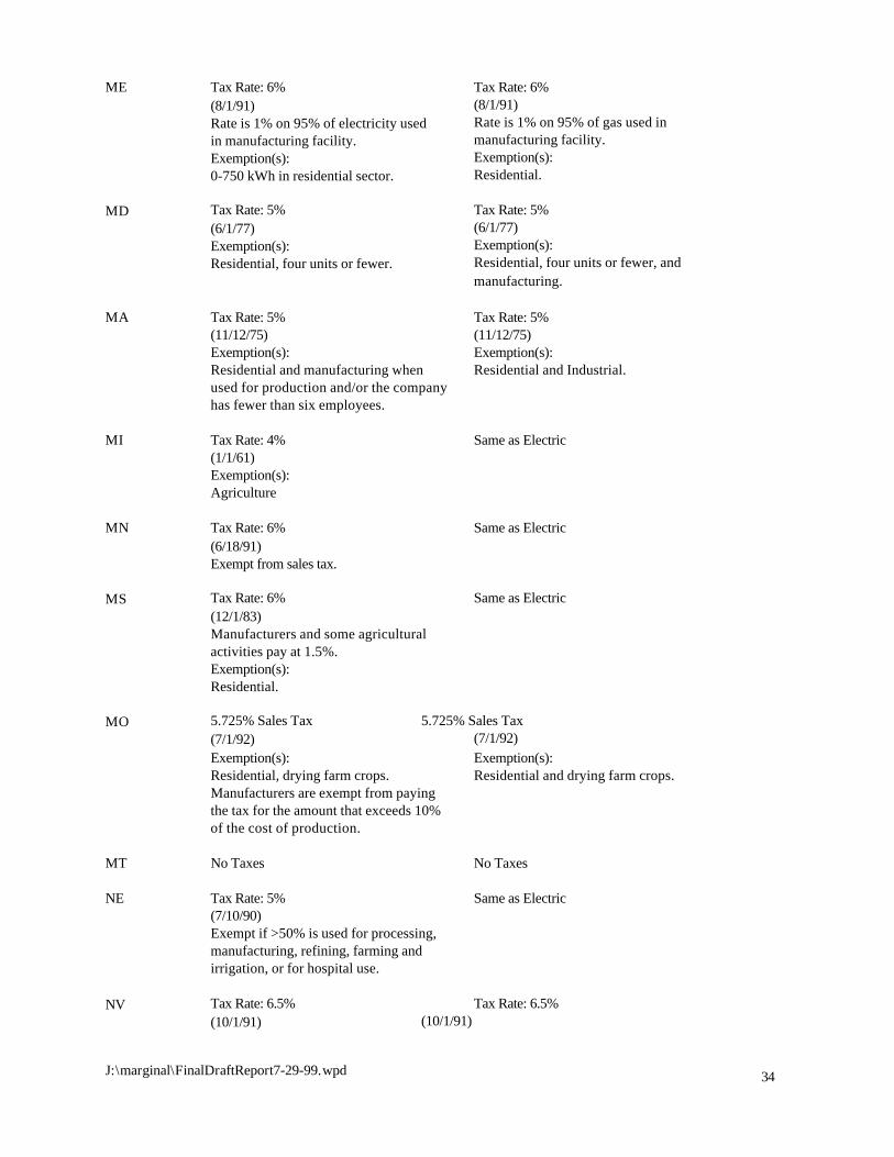
34J:\marginal\FinalDraftReport7-29-99.wpd
ME Tax Rate: 6% Tax Rate: 6%(8/1/91) (8/1/91)Rate is 1% on 95% of electricity used Rate is 1% on 95% of gas used inin manufacturing facility. manufacturing facility.Exemption(s): Exemption(s):0-750 kWh in residential sector. Residential.
MD Tax Rate: 5% Tax Rate: 5%(6/1/77) (6/1/77)Exemption(s): Exemption(s):Residential, four units or fewer. Residential, four units or fewer, and
manufacturing.
MA Tax Rate: 5% Tax Rate: 5%(11/12/75) (11/12/75)Exemption(s): Exemption(s):Residential and manufacturing when Residential and Industrial.used for production and/or the companyhas fewer than six employees.
MI Tax Rate: 4% Same as Electric(1/1/61)Exemption(s):Agriculture
MN Tax Rate: 6% Same as Electric(6/18/91)Exempt from sales tax.
MS Tax Rate: 6% Same as Electric(12/1/83)Manufacturers and some agriculturalactivities pay at 1.5%.Exemption(s):Residential.
MO 5.725% Sales Tax 5.725% Sales Tax(7/1/92) (7/1/92)Exemption(s): Exemption(s):Residential, drying farm crops. Residential and drying farm crops.Manufacturers are exempt from payingthe tax for the amount that exceeds 10%of the cost of production.
MT No Taxes No Taxes
NE Tax Rate: 5% Same as Electric(7/10/90)Exempt if >50% is used for processing,manufacturing, refining, farming andirrigation, or for hospital use.
NV Tax Rate: 6.5% Tax Rate: 6.5%(10/1/91) (10/1/91)
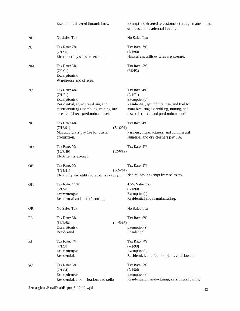
35J:\marginal\FinalDraftReport7-29-99.wpd
Exempt if delivered through lines. Exempt if delivered to customers through mains, lines,or pipes and residential heating.
NH No Sales Tax No Sales Tax
NJ Tax Rate: 7% Tax Rate: 7%(7/1/90) (7/1/90)Electric utility sales are exempt. Natural gas utilities sales are exempt.
NM Tax Rate: 5% Tax Rate: 5%(7/9/91) (7/9/91)Exemption(s):Warehouse and offices.
NY Tax Rate: 4% Tax Rate: 4%(7/1/71) (7/1/71)Exemption(s): Exemption(s):Residential, agricultural use, and Residential, agricultural use, and fuel formanufacturing assembling, mining, and manufacturing assembling, mining, andresearch (direct-predominant use). research (direct and predominant use).
NC Tax Rate: 4% Tax Rate: 4%(7/16/91) (7/16/91)Manufacturers pay 1% for use in Farmers, manufacturers, and commercialproduction. laundries and dry cleaners pay 1%.
ND Tax Rate: 5% Tax Rate: 5%(12/6/89) (12/6/89)Electricity is exempt.
OH Tax Rate: 5% Tax Rate: 5%(1/24/81) (1/24/81)Electricity and utility services are exempt. Natural gas is exempt from sales tax.
OK Tax Rate: 4.5% 4.5% Sales Tax(5/1/90) (5/1/90)Exemption(s): Exemption(s):Residential and manufacturing. Residential and manufacturing.
OR No Sales Tax No Sales Tax
PA Tax Rate: 6% Tax Rate: 6%(11/1/68) (11/5/68)Exemption(s): Exemption(s):Residential. Residential.
RI Tax Rate: 7% Tax Rate: 7%(7/1/90) (7/1/90)Exemption(s): Exemption(s):Residential. Residential, and fuel for plants and flowers.
SC Tax Rate: 5% Tax Rate: 5%(7/1/84) (7/1/84)Exemption(s): Exemption(s):Residential, crop irrigation, and radio Residential, manufacturing, agricultural curing,
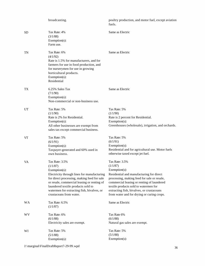
36J:\marginal\FinalDraftReport7-29-99.wpd
broadcasting. poultry production, and motor fuel, except aviationfuels.
SD Tax Rate: 4% Same as Electric(3/1/88)Exemption(s):Farm use.
TN Tax Rate: 6% Same as Electric(4/1/92)Rate is 1.5% for manufacturers, and forfarmers for use in food production, andfor nurserymen for use in growinghorticultural products.Exemption(s):Residential
TX 6.25% Sales Tax Same as Electric(7/1/90)Exemption(s):Non-commercial or non-business use.
UT Tax Rate: 5% Tax Rate: 5%(1/1/90) (1/1/90)Rate is 2% for Residential. Rate is 2 percent for Residential.Exemption(s): Exemption(s):All other businesses are exempt from Greenhouses (wholesale), irrigation, and orchards.sales tax except commercial business.
VT Tax Rate: 5% Tax Rate: 5%(6/1/91) (6/1/91)Exemption(s): Exemption(s):Taxpayer-generated and 60% used in Residential and for agricultural use. Motor fuelsown business. otherwise taxed except jet fuel.
VA Tax Rate: 3.5% Tax Rate: 3.5%(1/1/87) (1/1/87)Exemption(s): Exemption(s):Electricity through lines for manufacturing Residential and manufacturing for directfor direct processing, making feed for sale processing, making feed for sale or resale,or resale, commercial leasing or renting of commercial leasing or renting of launderedlaundered textile products sold to textile products sold to watermen for watermen for extracting fish, bivalves, or extracting fish, bivalves, or crustaceans
crustaceans from water. from water and for drying or curing crops.
WA Tax Rate: 6.5% Same as Electric(1/1/87)
WV Tax Rate: 6% Tax Rate 6%(6/1/88) (6/1/88)Electricity sales are exempt. Natural gas sales are exempt.
WI Tax Rate: 5% Tax Rate: 5%(5/1/88) (5/1/88)Exemption(s): Exemption(s):

37J:\marginal\FinalDraftReport7-29-99.wpd
Residential and farming: November Residential and farming: November through April;through April. commercial fishing, interstate and foreign commerce,
and railroads.
WY Tax Rate: 3% Same as Electric(7/1/67)Exemption(s):Manufacturing process, and agriculturaluse.
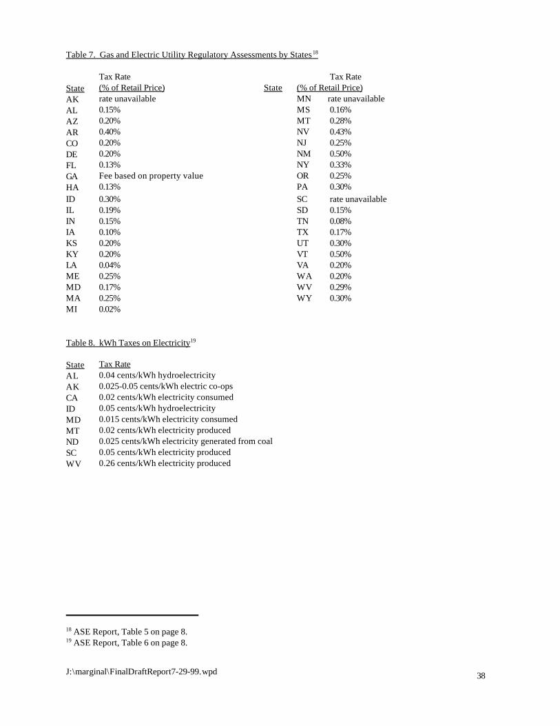
18 ASE Report, Table 5 on page 8.19 ASE Report, Table 6 on page 8.
38J:\marginal\FinalDraftReport7-29-99.wpd
Table 7. Gas and Electric Utility Regulatory Assessments by States18
Tax Rate Tax RateState (% of Retail Price) State (% of Retail Price)AK rate unavailable MN rate unavailableAL 0.15% MS 0.16%AZ 0.20% MT 0.28%AR 0.40% NV 0.43%CO 0.20% NJ 0.25%DE 0.20% NM 0.50%FL 0.13% NY 0.33%GA Fee based on property value OR 0.25%HA 0.13% PA 0.30%ID 0.30% SC rate unavailableIL 0.19% SD 0.15%IN 0.15% TN 0.08%IA 0.10% TX 0.17%KS 0.20% UT 0.30%KY 0.20% VT 0.50%LA 0.04% VA 0.20%ME 0.25% WA 0.20%MD 0.17% WV 0.29%MA 0.25% WY 0.30%MI 0.02%
Table 8. kWh Taxes on Electricity19
State Tax RateAL 0.04 cents/kWh hydroelectricityAK 0.025-0.05 cents/kWh electric co-opsCA 0.02 cents/kWh electricity consumedID 0.05 cents/kWh hydroelectricityMD 0.015 cents/kWh electricity consumedMT 0.02 cents/kWh electricity producedND 0.025 cents/kWh electricity generated from coalSC 0.05 cents/kWh electricity producedWV 0.26 cents/kWh electricity produced
Related Documents