Long-term Forecasting and Evaluation

Available online at www.sciencedirect.com

sting 23 (2007) 539–551www.elsevier.com/locate/ijforecast

International Journal of Foreca

Long-term forecasting and evaluation

Clive W.J. Granger a,1, Yongil Jeon b,⁎

a Department of Economics, University of California, San Diego, La Jolla, CA 92093-0508, United Statesb School of Economics, Sungkyunkwan University, 53 Myeongnyun-dong 3ga, Jongno-ku, Seoul, 110-745, South Korea

Abstract

Looking ahead thirty years is a difficult task, but is not impossible. In this paper we illustrate how to evaluate such long-termforecasts. Long-term forecasting is likely to be dominated by trend curves, particularly the simple linear and exponential trends.However, there will certainly be breaks in their parameter values at some unknown points, so that eventually the forecasts willbe unsatisfactory. We investigate whether or not simple methods of long-run forecasting can ever be successful, after one takesinto account the uncertainty level associated with the forecasts.© 2007 International Institute of Forecasters. Published by Elsevier B.V. All rights reserved.

JEL classification: C5

Keywords: Long-term trend fitting; Forecasting evaluation; Density forecasting

1. Introduction

Suppose that one was asked to forecast the generalstate of the economy of the world in the year 2037using data available in the year 2007. It would be adaunting task. Most of the commonly used forecastingtechniques would be irrelevant. If a model assumesstationarity, the long run forecast is just the mean of theseries. If the model assumes a unit root without drift,then the long run forecast is essentially the most recentvalue of the series. A unit root process with driftsimply gives a long run forecast that is a linear trend.

⁎ Corresponding author. Tel.: +82 2 760 0487; fax: +82 2 744 5717.E-mail addresses: [email protected] (C.W.J. Granger),

[email protected] (Y. Jeon).1 Tel.: +1 858 534 3856; fax: +1 858 534 7040.

y

0169-2070/$ - see front matter © 2007 International Institute of Forecastedoi:10.1016/j.ijforecast.2007.07.002

Long-term forecasting will probably be dominated bytrend curves, particularly the simple linear and expo-nential trends. Unfortunately, there will also certainlybe breaks in their parameter values at unknown points,so that eventually the forecasts will be unsatisfactory.An objective of this paper is to investigate whether ornot simple methods of long-run forecasting can besuccessful, after one fully considers the uncertaintiesassociated with the forecasts.

There are various different approaches to long-runforecasting. Examples are:

(1) “The World Economy. History and Prospects” byRostow (1978), who views the past to look into thefuture, and considers the stages of economicgrowth (in a similar fashion to the familiar stagesof demographic change), the trends and the cycles,

rs. Published by Elsevier B.V. All rights reserved.

540 C.W.J. Granger, Y. Jeon / International Journal of Forecasting 23 (2007) 539–551

with both short and long periods, particularly theKontratieff Wave. The book includes few actualforecasts that can be evaluated.

(2) In “Towards the Year 2000” edited by DanielBell (1968), which is a report by the AmericanAcademy's Commission on the Year 2000,forty-three high quality contributors, all malesapart from Margaret Mead, contribute intellec-tual essays and discussions. These producesensible accounts of many topics, viewed fromseveral perspectives, but fail to reach manyconclusions and give no specific forecasts.

(3) “The Limits to Growth” by Meadows, Mea-dows, Randers, and Behrens (1972) containsspecific forecasts, called scenarios, which arederived from a complicated, possibly non-linear,feedback model. This model can produceinitially exponential trends which may eventu-ally clash and result in a collapse of theeconomy. A later evaluation, “Beyond theLimits” by Meadows, Meadows, Randers, andTinbergen (1992) displays results from thirteenscenarios, of which three reach a maximumupper limit for the material standard of livingaround the year 2000, nine produce collapsesstarting soon after 2000, and one expands livingstandards until 2040 and then collapses. Theresults are not robust to small changes in theassumptions used in the models.

(4) “The Year 2000” by Kahn and Wiener (1967),which is the subject of the discussion in Section 2,bases forecasts on trends of many kinds, considersscenarios about how various movements willinteract in the future, and includes the impact ofscientific development.2 The study came from theHudson Institute, a private non-profit public policy“think tank” that is still active. The objective was

2 Kahn and Wiener use a variety of forecasting techniques, butparticularly:

(a)Trendline fitting for population and economic forecasts. Thisproduced a mixed success: good if a satisfactory trend curve ischosen, but otherwise quite incorrect.

(b)Scenarios thinking about plausible futures. Kahn and Wienerare again successful on occasions, but miss some substantial futuredevelopments.

(c)A form of Delphi for looking at scientific breakthroughs,which involves talking to prominent scientists. This technique isoften successful, as some current trends do continue, but othersprove to be dead ends.

to use the data available in 1966 or so to forecastthe society, and particularly the economy, aroundthe year 2000. When one forecasts as far as thirty-three years ahead, it should not be expected thatthe forecastswill be precise either in size or in date.In 1967 theywould not be expected tomake usefulforecasts of, say, unemployment or inflation forNew York or London for the year 2000. It wouldbe as unrealistic as our making such forecasts in2000 for the year 2033. It is difficult enoughmaking forecasts for economic variables over aone year horizon.3 Some growth rates can beexpected to remain constant over a thirty yearperiod, while some could decline because ofchanging tastes or scarcity of resources. Othergrowth rates could increase because of newopportunities and scientific advances. The realforecasting skill comes in deciding what arereasonable or likely changes in the growth rates.4

This paper unfolds as follows. Section 2 discussesthe book by Kahn and Wiener (1967), which illustratesthat long-range forecasting is difficult but notimpossible, and provides a useful template of how toapproach the task. We illustrate the evaluation of theirlong-term forecasts of science and technology, and theU.S. population and economy. In the remainder of ourdiscussion we examine the properties of trend fitting ingreater depth. This is hardly a new use, but it is onethat has not been systematically explored for its long-run forecasting abilities. Section 3 considers the post-sample evaluation of four different trend fitting curvesfor total U.S. personal consumption, where the initialforecasting was done in Granger (1980, 1989). Section4 employs two popular trend fitting models, a randomwalk model with drift and a trend-stationary model(with equal weights and with exponential decliningweights). Although the two models indicate similarlong-term mean forecasts, their confidence intervalsdiverge as the forecasting horizons increase. Using theuncertainty measure helps to differentiate between two

3 Some variables, such as population, change fairly slowly andponderously, while others, such as GDP, change in a steady fashion.These are thus candidates for numerical forecasts, and hence forevaluation.4 When considered together, one gets a diverse, varied set of

trends, described frequently in Kahn and Wiener by the delightfullyold-fashioned term “multifold trends.”

6 Examples of “half-successes” by our chosen scheme areimproved acceptability of the “change” of sex of children and/or

541C.W.J. Granger, Y. Jeon / International Journal of Forecasting 23 (2007) 539–551

similar models in the trend fitting. Section 5 presentsour conclusions.

2. Forecasting science — an evaluative review ofKahn and Wiener (1967)

The activities of “futurists” in the 1960s could bedivided into “hard” and “soft” components. The hardside dealt with technological forecasting, often based onforecasts of scientific developments, as in Gabor (1963),or on trend fitting, to extrapolate measures of technicalability, such as computer speed or the maximum speedof aircraft. The soft side largely consisted of scenariowriting, in which an attempt wasmade to describe how afuture society would look if various trends continuedand interacted with each other and with expectedscientific discoveries.

It is useful to consider Kahn and Wiener's study insome detail, because it illustrates the possibility ofmaking some worthwhile long-run forecasts and theobvious difficulties of doing so. To be sensible, thesociety in the scenario has to fit together; that is, it mustbe coherent. A central, or “surprise-free” scenario istaken to be the most likely, but a variety of more extremepossible scenarios can also be envisioned, such as theweakening of communism, the breakdown of democra-cy, or the aftermath of a nuclear war. About half of Kahnand Wiener (1967) is concerned with such scenarios,which make interesting enough reading, rather likeviewing George Orwell's “1984” in 1960, but suchprojections or forecasts are virtually impossible toevaluate. The surprise-free scenario for 2000 is roughlycorrect in some respects but quite wrong in others. Partof the problem is that a scenario does not forecast aparticularly tight period, such as the year 2000, but rathera longer time period, say 1975 to 2010. For example,there is a great deal of attention paid to weapons andmilitary spending, which was important for much of theintervening period, but was less so by 2000.

Hard forecasts are rather easier to evaluate, al-though difficulties remain.5 The authors provide a list

5 The first chapter lists a number of basic trends, most of whichproved to be correct, and several of which will be relevant in thefuture. Also in chapter one, the classification of future solutions intogroups from “pre-industrial” to “post-industrial” need redefining butremains useful. The “canonical variables” from the “standard world”from Chapter 6 are also helpful in organizing one's thinking.

of 100 “Technical Innovations Very Likely in the LastThird of the Twentieth Century.” Using entirelypersonal subjective criteria, we would judge thatthirty-five of these innovations have occurred, forty-eight have not, fourteen have partially occurred (thatis, they are in the very early stages) and three could notbe classified because their statements were unclear.Some examples of successful forecasts are morereliable and longer-range weather forecasting; exten-sive and intensive use of high altitude cameras; newtechniques for cheap, convenient, and reliable birthcontrol; a general and substantial increase in lifeexpectancy; “high quality” medical care for undevel-oped areas; automated grocery and department stores(becoming used); and home computers to “run”households and communicate with the outside world.

Examples of forecasts that are unsuccessful so farare intensive and/or extensive expansion of tropicalagriculture and forestry (chopping down trees does notqualify); some control of weather and/or climate; newand more reliable “educational” and propagandatechniques for affecting human behavior, both publicand private; human hibernation for extensive periods(months to years); the capability to choose the sex ofunborn children (not counting selective abortion); newtechniques and institutions for the education ofchildren (computers?); and physically non-harmfulmethods of over-indulging.

Some of these examples illustrate how difficult it isto interpret the forecast and judge whether it issuccessful or not.6 We have listed just a few of theone hundred innovations given in the book asexamples. If our personal classifications are accepted,it is unclear whether having thirty-five out of onehundred correct is considered a success, as there isnothing with which to compare it. Many of the lesssuccessful forecasts have a problem with time; these

adults; permanent manned satellites and lunar installations, andinterplanetary travel; and flexible penology without using prisons.Examples of forecasts that we could not judge include new orimproved super performance fabrics (papers, filters, plastics); agreater use of underground buildings; and major improvements inearth moving and construction equipment generally. It is unclearhow one evaluates words such as “new or improved,” “greater use”or “major improvements.”

542 C.W.J. Granger, Y. Jeon / International Journal of Forecasting 23 (2007) 539–551

innovations seem likely to come about in the nextdecade or so.

The authors also list twenty-five “less likely butimportant possibilities”, and a further list of “ten farout possibilities,” none of which have occurred by theyear 2000. The first list includes, for example, roomtemperature superconductors; the conversion of mam-mals (humans?) to being fluid breathers; and atechnological equivalent of telepathy. The onlyexample that comes close to occurring is the predictionof the use of automated freeways. The “far-out” listincludes anti-gravity, interstellar travel, and extremelycheap electricity.

Some scientific advances that have happened but donot appear on the lists are cloning, the human DNAgenome sequence map, and the development of thehigh-production rice and wheat which produced the“green revolution” that helped feed the world'sincrease in population. The World Wide Web wasnot specifically forecast, but the use of fast homecomputers, linked together, and the widespreadavailability of all the information “in the Library ofCongress” is discussed. With all forms of technolog-ical forecasting, the forecasts are about what will bepossible rather than how this will be achieved. Thus,although the web itself and its full implications werenot forecast in the book, many of the basic propertiesof the system were indicated.7

Kahn and Wiener (1967) contains forecasts ofpopulation, GNP, and GNP per capita for the U.S. andseveral other countries to roughly the year 2000. For theU.S., a number of other economic measures are alsoforecast. On some occasions, low, middle, and highforecasts are provided to suggest some kind of uncertaintyrange, although these are not specific confidenceintervals. In what follows, some of the tables arereproduced in a growth rate form, with “actual” growthrate values for the year 2000 added. Most “actuals” areavailable from the 2002 Statistical Abstract of the UnitedStates(www.census.gov) or the World Population DataSheet, 2002, from the Population Reference Bureau.

The GNP per capita in the World Population DataSheet is in 2000 US$. To convert to 1965 US$ wemultiply by 0.2 (as the average inflation rate between

7 The chapter on science and technology pays particular attentionto nuclear energy, lasers, and holography, choices which now seemrather strange. All are important in differing degrees, but for thelatter two, less than was anticipated in 1967, we believe.

1965 and 2000 was about 4%). It is seen that theforecast populations are generally higher than theactual populations, and the GNP/capita forecasts aremuch too high, as is shown in Table 1. The samepatterns occur with major individual countries, as isshown in Table 2. It is worth noting that two majorcountries in the original table, the Soviet Union andGermany, have changed dramatically. An unintendedforecast being made by the book's authors was thatcountries would stay unchanged.

The country-specific data shown in Table 3indicates that, for GNP per capita for fourteen othercountries, the ratio of actual/forecast values varies from0.09 to 1.9, which is a wide range. Table 3 illustratesthat only four forecasts were too high. Table 4 showsthat, in general, the forecasts for the U.S. were too high,being optimistic in forecasting components of the U.S.GNP per capita. In addition, GNP and two-thirds of thecomponents were forecast too high.

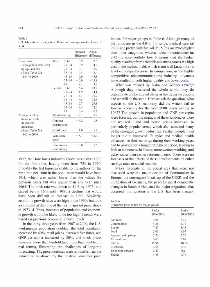
Kahn and Wiener also forecast labor marketvariables, shown in Table 5. Men actually participatesomewhat less than expected, but women participate toa much greater extent. Although this is not shown, it isparticularly the case for unmarried women, eventhough married women's participation rates are alsohigh relative to expectations. Kahn and Wiener makecontinued reference to declines in the work week, extravacations and days of rest, and general increases inleisure. The problem of how society would cope withthe large amounts of leisure time that its workerswould enjoy around the year 2000 was a popular topicamongst forecasters in the 1960s. This “difficulty”really has not occurred, particularly in the UnitedStates, as the above figures show, with the hours ofwork in 2000 being similar to those in 1965, except forthe Retail Trade which has turned to a greater use ofpart-time workers. Other developed economies do notfollow quite the same pattern, however.

As an article in the Time magazine (13 June 2000)reported, vacation times taken as mandated varygreatly across the more-developed countries, from30 days a year in France, Austria, Denmark, Spain andSweden, down to 18 in Germany and 16 in the USA.The fact that the numerical forecasts are not exactly thesame as the actual figures for (around) 2000 should notbe interpreted negatively. It is unclear whether anyonecould have done much better. Forecasting with perfecthindsight is all too easy, and is not to be trusted.

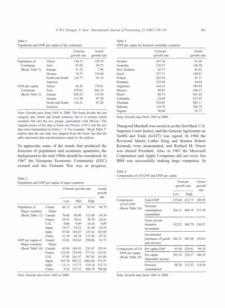
Table 1Population and GNP per capita of the continents

Forecastgrowth rate

Actualgrowth rate

Population ofContinents(Book Table 3)

Africa 150.72 158.79Asia 95.92 94.75Europe 31.32 7.99Oceana 78.57 119.60North and SouthAmerica

116.77 81.76

GNP per capitaContinents(Book Table 3)

Africa 96.45 178.01Asia 279.61 463.16Europe 269.25 135.94Oceana 115.50 87.70North and SouthAmerica

116.21 87.28

Note: Growth rates from 1965 to 2000. The book divides the lascategory into North and South America, but it is unclear whichcountries fall into the two groups, particularly with Mexico. Theoriginal source of the data is Kahn and Wiener (1967), but the rawdata were manipulated in Tables 1–6. For example, “Book Table 3”implies that the raw data was adapted from the book, but that thetable represents data transformations made by the authors.

Table 2Population and GNP per capita of major countries

Forecast growth rate Actualgrowthrate

Low Mid High

Population ofMajor countries(Book Table 12)

UnitedStates

48.72 63.08 85.64 44.79

Canada 70.00 90.00 115.00 56.39France 20.41 30.61 38.78 20.41U.K. 0.00 9.09 16.36 9.09Japan 18.37 25.51 41.84 29.29India 87.68 102.87 131.62 105.89China 31.39 68.34 111.92 67.22

GNP per capita ofMajor countries(Book Table 14)

UnitedStates

33.82 185.63 250.86 91.73

Canada 63.96 186.93 251.87 120.54France 132.85 254.99 371.41 153.85U.K. 97.89 261.97 367.85 161.09Japan 365.58 902.33 1066.86 531.97India − 13.13 172.73 310.10 372.73China 8.16 227.55 888.78 700.00

Note: Growth rates from 1965 to 2000.

Table 3GNP per capita for fourteen contender countries

Forecastgrowth rate

Actualgrowth rate

Sweden 247.58 91.99Australia 129.57 148.58New Zealand 65.37 91.82Israel 337.71 189.81Poland 282.54 87.11Romania 325.89 68.03Argentina 164.23 389.84Mexico 49.45 286.37Brazil 80.71 421.43Columbia 29.60 337.55Thailand 219.05 903.17Pakistan 119.78 308.79Nigeria 50.60 92.77

Note: Growth rates from 1965 to 2000.

543C.W.J. Granger, Y. Jeon / International Journal of Forecasting 23 (2007) 539–551

t

To appreciate some of the trends that produced theforecasts of population and economic quantities, thebackground to the mid-1960s should be considered. In1967 the European Economic Community (EEC)existed and the Vietnam War was in progress;

able 4omponents of US GNP and GNP per capita

Forecastgrowth rate

Actualgrowthrate

Low High

omponentsof US GNP(Book Table 26)

Total GNP 219.68 432.75 189.95

Personalconsumptionexpenditure

236.11 460.19 211.50

Gross privatedomesticinvestment

192.52 388.79 230.37

Governmentpurchases of goodsand services

202.21 403.68 156.03

omponents of USGNP per capita(Book Table 29)

Per capita GNP 95.60 229.81 99.35

Per capitadisposable income

103.32 238.17 106.55

Personalconsumption

98.20 215.32 114.58

ote: Growth rates from 1965 to 2000.

ThurgoodMarshall was sworn in as the first black U.S.Supreme Court Justice; and the General Agreement onTariffs and Trade (GATT) was signed. In 1968 theReverend Martin Luther King and Senator RobertKennedy were assassinated, and Richard M. Nixonwas elected President. Also, in 1967 the MicrosoftCorporation and Apple Computers did not exist, butIBM was successfully making large computers. In

TC

C

C

N

able 5.S. labor force participation: Rates and average weekly hours ofork

Forecastdifference

Actualdifference

abor forceParticipation Rates (%)by age and sex(Book Table 22)1964 to 2000

Male Total 0.9 − 2.520−24 0.9 − 4.025–34 0.1 − 2.735–44 0.4 − 3.445–54 0.6 − 5.855–64 − 0.9 − 16.865+ − 8.1 − 9.6

Female Total 5.4 23.220–24 4.9 24.125–34 4.1 39.235–44 6.5 32.545–54 10.7 25.855–64 9.4 12.065+ 0.4 − 0.2

verage weeklyhours of workin selectedindustries(Book Table 23)1965 to 2000

Manufacturing − 9.1 0.2

Contractconstruction

− 6.2 1.8

Retail trade − 4.0 − 5.4

Wholesaletrade

− 8.7 − 2.0

Bituminouscoal mining

− 10.0 5.5

544 C.W.J. Granger, Y. Jeon / International Journal of Forecasting 23 (2007) 539–551

TUw

L

A

Table 6Consumer price index by major groups

Ratios1996/1965

Ratios2000/1965

All items 4.98 5.47Commodities 4.36 4.77Energy 7.47 8.45Food 3.01 4.05Apparel and upkeep 2.24 2.76Medical care 5.67 6.08Fuel oil 15.96 18.24Electricity 4.24 3.32Telephone services 2.42 NAShelter 4.88 4.76

1972, the Dow Jones Industrial Index closed over 1000for the first time, having risen from 753 in 1970.Probably the last figure available to the authors for thebirth rate per 1000 in the population would have been19.4, which was rather lower than the values forprevious years but was higher than any year since1965. The birth rate was down to 14.8 by 1973, andstayed below 16.0 until 1988, a decline that wouldhave been difficult to forecast in 1966. Similarly,economic growth rates were high in the 1960s but tooka strong hit at the time of the first major oil price shockin 1973–4. Thus, forecasts of population and econom-ic growth would be likely to be too high if trends werebased on previous economic growth levels.

In the thirty-three years from 1967 to 2000, the U.S.working-age population doubled, the total populationincreased by 40%, retail prices increased five times, realGNP per capita increased by 80%, and stock pricesincreased more than ten-fold (and more than doubled inreal terms), illustrating the challenges of long-runforecasting. The price increases were not uniform acrossindustries, as shown by the relative consumer price

indices for major groups in Table 6. Although many ofthe ratios are in the 4.0 to 5.0 range, medical care (at9.06), and particularly fuel oil (at 15.96), aremuch higherthan other categories, whereas telecommunications (at2.42) is note-worthily low. It seems that the higherquality resulting from scientific advances comes at a highcost in the medical field, which is not well known for itslevel of competitiveness. In comparison, in the highlycompetitive telecommunications industry, advanceshave resulted in both higher quality and lower costs.

What was missed by Kahn and Wiener (1967)?Although they discussed the whole world, they doconcentrate on the United States as the largest economy,and we will do the same. Here we ask the question, whataspects of the U.S. economy did the writers fail toforecast correctly for the year 2000 when writing in1967? The growth in population and GNP per capitawere forecast, but the impacts of these tendencies werenot realized. Land and house prices increased inparticularly popular areas, which also attracted manyof the strongest growth industries. Further, people livedlonger due to improved life styles and medical healthadvances, so their earnings during their working yearshad to provide for a longer retirement period, leading tolittle or no increase in leisure,morewomenworking, anddelay rather than earlier retirement ages. There were noforecasts of the effects of these developments on eithersavings rates or social security.

Major forecasts in the social area that were notdiscussed were the major decline of Communism inEurope, the consequent break-up of the USSR and theunification of Germany, the peaceful racial democraticchanges in South Africa, and the major migrations thatoccurred. Immigration in the U.S. has been a major

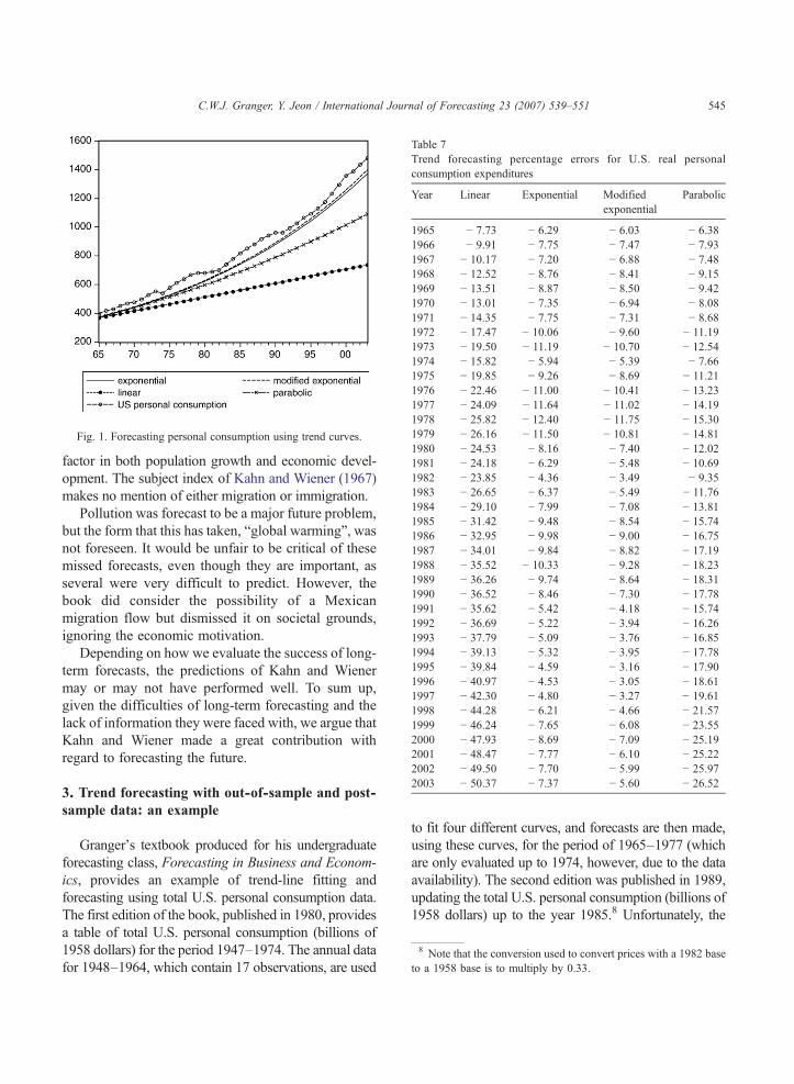
Table 7Trend forecasting percentage errors for U.S. real personaconsumption expenditures

Year Linear Exponential Modifiedexponential

Parabolic

1965 − 7.73 − 6.29 − 6.03 − 6.381966 − 9.91 − 7.75 − 7.47 − 7.931967 − 10.17 − 7.20 − 6.88 − 7.481968 − 12.52 − 8.76 − 8.41 − 9.151969 − 13.51 − 8.87 − 8.50 − 9.421970 − 13.01 − 7.35 − 6.94 − 8.081971 − 14.35 − 7.75 − 7.31 − 8.681972 − 17.47 − 10.06 − 9.60 − 11.191973 − 19.50 − 11.19 − 10.70 − 12.541974 − 15.82 − 5.94 − 5.39 − 7.661975 − 19.85 − 9.26 − 8.69 − 11.211976 − 22.46 − 11.00 − 10.41 − 13.231977 − 24.09 − 11.64 − 11.02 − 14.191978 − 25.82 − 12.40 − 11.75 − 15.301979 − 26.16 − 11.50 − 10.81 − 14.81Fig. 1. Forecasting personal consumption using trend curves.

545C.W.J. Granger, Y. Jeon / International Journal of Forecasting 23 (2007) 539–551

1980 − 24.53 − 8.16 − 7.40 − 12.021981 − 24.18 − 6.29 − 5.48 − 10.691982 − 23.85 − 4.36 − 3.49 − 9.351983 − 26.65 − 6.37 − 5.49 − 11.761984 − 29.10 − 7.99 − 7.08 − 13.811985 − 31.42 − 9.48 − 8.54 − 15.741986 − 32.95 − 9.98 − 9.00 − 16.751987 − 34.01 − 9.84 − 8.82 − 17.191988 − 35.52 − 10.33 − 9.28 − 18.231989 − 36.26 − 9.74 − 8.64 − 18.311990 − 36.52 − 8.46 − 7.30 − 17.781991 − 35.62 − 5.42 − 4.18 − 15.741992 − 36.69 − 5.22 − 3.94 − 16.261993 − 37.79 − 5.09 − 3.76 − 16.851994 − 39.13 − 5.32 − 3.95 − 17.781995 − 39.84 − 4.59 − 3.16 − 17.901996 − 40.97 − 4.53 − 3.05 − 18.611997 − 42.30 − 4.80 − 3.27 − 19.611998 − 44.28 − 6.21 − 4.66 − 21.571999 − 46.24 − 7.65 − 6.08 − 23.552000 − 47.93 − 8.69 − 7.09 − 25.192001 − 48.47 − 7.77 − 6.10 − 25.222002 − 49.50 − 7.70 − 5.99 − 25.972003 − 50.37 − 7.37 − 5.60 − 26.52

8 Note that the conversion used to convert prices with a 1982 baseto a 1958 base is to multiply by 0.33.

factor in both population growth and economic devel-opment. The subject index of Kahn and Wiener (1967)makes no mention of either migration or immigration.

Pollution was forecast to be a major future problem,but the form that this has taken, “global warming”, wasnot foreseen. It would be unfair to be critical of thesemissed forecasts, even though they are important, asseveral were very difficult to predict. However, thebook did consider the possibility of a Mexicanmigration flow but dismissed it on societal grounds,ignoring the economic motivation.

Depending on how we evaluate the success of long-term forecasts, the predictions of Kahn and Wienermay or may not have performed well. To sum up,given the difficulties of long-term forecasting and thelack of information they were faced with, we argue thatKahn and Wiener made a great contribution withregard to forecasting the future.

3. Trend forecasting with out-of-sample and post-sample data: an example

Granger's textbook produced for his undergraduateforecasting class, Forecasting in Business and Econom-ics, provides an example of trend-line fitting andforecasting using total U.S. personal consumption data.The first edition of the book, published in 1980, providesa table of total U.S. personal consumption (billions of1958 dollars) for the period 1947–1974. The annual datafor 1948–1964, which contain 17 observations, are used

l

to fit four different curves, and forecasts are then made,using these curves, for the period of 1965–1977 (whichare only evaluated up to 1974, however, due to the dataavailability). The second edition was published in 1989,updating the total U.S. personal consumption (billions of1958 dollars) up to the year 1985.8 Unfortunately, the

9 Granger (1980) estimates the linear function using OLS C(t) =191+9.69t which is very similar to the two-point estimates. Grange(1989, page 37) claims that using the OLS estimated exponentiafunction gives forecasting values that are too high, and thus that theunsophisticated estimation of the two point method produces the betteforecasts, although this is not what we would usually expect to occur.

Fig. 2. Trend stationary forecasting: the case of the U.S.

546 C.W.J. Granger, Y. Jeon / International Journal of Forecasting 23 (2007) 539–551

second edition did not expand the fitting period, keepingthe same estimation period of 1948–1964, and thusproviding the same parameters for the four curves.However, the evaluation is made for the updated sampleperiod of 1965–1988.

The four different trend curves fitted in Granger(1980, 1989) are the linear, exponential, parabolic, andmodified exponential curves, although trend-curvefitting methods rarely have any solid economic theoryunderlying the forecasts. In the first attempt, Granger(1980) uses a much simpler (but possibly suboptimal)estimation method, where the averages of five adjacentpoints are used to fit the curves. A three-point methodis used for fitting the parabolic curve and the modifiedexponential curve. Each of three points is the weightedaverage of the first five terms, the weighted average ofthe middle five terms, and the weighted average of thelast five terms. Two points, which are the weightedaverage of the first five terms and the last five terms,

completely determine the parameters of the twoparameter curves, the linear straight line and theexponential curve. The estimated parameters fromusing either the two- or the three-point method are 9

(i) the linear line, C(t)=a+b·t=192.6+9.687t

(ii) the exponential curve, C(t)= exp(a+b·t) = exp(5.3033+0.0343t)

(iii) the parabolic curve, C(t)= a+b·t+c·t2 =201.96+6.449t+0.1675t2

(iv) the modified exponential curve, C(t)= a+b·rt=3.131+197.79 (1.0355)t.

rl

r

Fig. 3. Trend stationary forecasts with exponential weights: the case of the U.S.

547C.W.J. Granger, Y. Jeon / International Journal of Forecasting 23 (2007) 539–551

Granger (1980, pp. 35–36) reports that, over theestimation and out-of-sample periods, the straight lineis the worst approximation, while the other threecurves are indistinguishable. Each curve's downwardbias for the out-of-sample forecasting period from1965 to 1974 was noted. Later, Granger (1989, p. 37)claims that the exponential and modified exponentialforecasts are almost identical, and that both aresuperior to those of the linear and parabolic curves,with acceptable levels of error such as 1%–7%.

In this paper, the annual data of real personalconsumption expenditures is updated to 2003 (bil-lions of chained 2000 dollars) from the FederalReserve Bank of St. Louis.10 Using post-sample data,the trend forecasting is carried out for four different

10 The conversion used for converting prices with a 2000 base to a1958 base is to multiply by 0.20117, after comparing the commondata between 1947 and 1974.

methods, shown in Fig. 1, using the parameterestimates from the 1980 book. The forecastingevaluation is performed using

error ¼ ðforecast� actualÞactual

� 100:

Table 7 shows the out-of-sample forecast percent-age errors. These values increase monotonically for thelinear and parabolic curves, but not for two exponen-tials. Over a 39 year period, the simple exponential hasa percentage error of less than 12.40 on all occasions,and for 23 horizons is less than 8% wrong. Themodified exponential percentage error is always lessthan that of the simple exponential, with 28 horizonsunder 8%. The most surprising statistic is that themodified exponential curve has had single-digitpercentage errors since 1980, and has been at orbelow 7.09 since 1981. Thus, it appears that this very

Fig. 4. Differenced stationary forecasting: the case of the U.S.

548 C.W.J. Granger, Y. Jeon / International Journal of Forecasting 23 (2007) 539–551

simple trend model can effectively forecast thisparticular economic series at least forty years ahead.

These two exponential curves can be written asγ+α ·βt, where for the exponential, γ=0, α= ea,β= eb, and for the modified exponential, γ=a, α=b,r=β. Thus, the modified exponential is superior,because it adds a further, and useful, coefficient. It isnevertheless worth noting that in Table 7, all of theerrors in the exponential columns are negative,suggesting that the modified exponential wouldhave done even better if the original estimate of γhad been larger. These results are also easily seen inFig. 1. The superiority of the exponential and themodified exponential are due to the relatively stablegrowth rate of consumption. The level of consump-tion, however, is not easily forecastable due to itsnon-stationarity.

4. Long-term forecast evaluation with uncertainty

In this section we consider the two simplest modelsfor long-term trend forecasts, a stochastic randomwalk model with drift and a deterministic trend-stationary model. These two empirical models indicatesimilar means, but the confidence intervals changedifferently as we forecast at longer horizons. Thedistinction between difference stationary and trendstationary models has been debated. Our simplest formof the random walk model with drift consists of a non-zero mean and a shock, while expanding theconfidence interval over forecasting horizons. Atrend stationary model contains a linear time trendand a white noise innovation, where the confidenceinterval does not change over the different horizons.Thus, the uncertainty is another way to differentiate

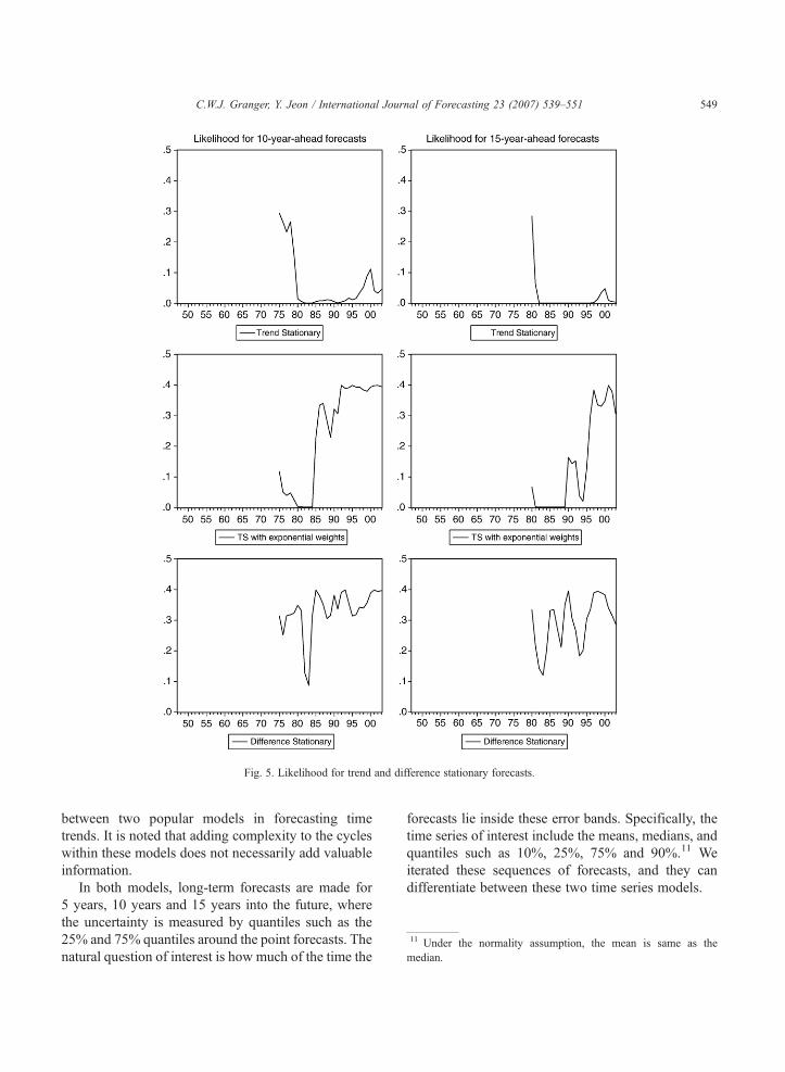
Fig. 5. Likelihood for trend and difference stationary forecasts.

11 Under the normality assumption, the mean is same as themedian.

549C.W.J. Granger, Y. Jeon / International Journal of Forecasting 23 (2007) 539–551

between two popular models in forecasting timetrends. It is noted that adding complexity to the cycleswithin these models does not necessarily add valuableinformation.

In both models, long-term forecasts are made for5 years, 10 years and 15 years into the future, wherethe uncertainty is measured by quantiles such as the25% and 75% quantiles around the point forecasts. Thenatural question of interest is how much of the time the

forecasts lie inside these error bands. Specifically, thetime series of interest include the means, medians, andquantiles such as 10%, 25%, 75% and 90%.11 Weiterated these sequences of forecasts, and they candifferentiate between these two time series models.

550 C.W.J. Granger, Y. Jeon / International Journal of Forecasting 23 (2007) 539–551

For the trend stationary model, we estimate thelinear time trend and the residual variance from in-sample data, since the series contains a deterministictrend accounting for the sustained increase over timeplus a stationary random disturbance term. That is,

yt ¼ aþ bdt þ et;

where et is a white noise with zero mean andσe2 variance.

Thus the h-step-ahead forecast is fn;h ¼ aþbðnþ hÞ,and its forecast error isV(en,h)=σe

2. Based on the data andmodel information, we can form density forecasts, andthus quantiles. Fixing the starting year, we move inone year increments and continue iterating this cycle.Alternatively, rather than putting equal weights onhistorical data, exponentially decreasing weights areused instead. That is, we choose a andb to make the sumof discounted squared residuals as small as possible:

XT

t¼1

kT�tðyt � a�bdtÞ2:

The value of λ=0.8 is used in an exploratory study,while λ=1 leads to ordinary least squares estimation.After fixing the starting year again, we move inone year increments of T and continue iterating thiscycle until the last observed year.

For the randomwalk model with drift, the wanderingassociated with the random walk is dominated by thepositive drift term. We take the first difference of arandom walk series, and form the drift and residuals.Then we have the difference stationary model being

yt ¼ yt�1 þ mþ et;

where εt is a white noise with zero mean and varianceσε2.

Therefore, the h-step-ahead forecast is gn;h ¼ hd mþ yn,and its forecast errors are V(εn,h)=h ·σε

2, which increasesas the forecast horizon h increases.

The data used is the annual real gross domesticproduct for the United States (billions of chained 2000dollars) between 1929 and 2003, obtained from theFederal Reserve Bank of St. Louis.12 Data from fiveother countries are also considered.13 Logs are taken

12 http://research.stlouisfed.org/fred2/series/GDPCA.13 The data for the other countries, including Australia (1950–2003), Japan (1950–2002), France (1950–2003), Germany (1950–2003), and the United Kingdom (1950–2003) are obtained from theIMF's International Financial Statistics. The analysis of thesecountries is available upon request.

before modeling the series. The first models areestimated using data from 1947 (1950 for the othercountries) to 1965, and then forecasting one year aheadfrom 1966, five years ahead from 1970, ten years aheadfrom 1975, and fifteen years ahead from 1980. Theresidual variances are also calculated and used forbuilding the 5%and 95%quantiles by using the standardnormality assumption. The procedure is iterated byone year increments from a fixed starting year, untilforecasts for the year 2003 are reached for eachforecasting horizon. The U.S. results are shown inFigs. 2, 3 and 4. The likelihoods observed as calculatedfrom the normality assumption are shown in Fig. 5.

Our discussion will concentrate on the ten and fifteenyear forecasts. Fig. 2 and 4 suggest that the two simplemodels being considered are not easy to differentiatebetween in terms of the central ormean forecast, but theydo differ substantially in terms of the spread, and thus inlikelihood, as seen in Fig. 5. Over both the ten- andfifteen-year horizons, both models consistently forecastquite well, but for this example, the random walk withdrift is superior. The actual GDP is quite close to theforecast mean and well within the confidence intervals.This is not so obviously the case with the linear model.

The exercises using data from other countries provedto be much less satisfactory, as these GDP growth rateswere much less nearly constant. By giving recent valuesof the data fitting period higher weight in the estimationmethod than the earlier data, improved forecasts wereobtained, but when a substantial change in growthoccurs several years in the future, it is clear that no trendcurve method will perform very well. To sum up, theresults illustrate the superiority of the random walk withdrift, as it has more realistic confidence intervals.

These confidence intervals have ignored “parame-ter uncertainty”, as we follow the standard forecastingprocedure of estimating a model and then using it toforecast, ignoring the fact that its parameters areestimated. The model is a tool, and when it is used weare not considering all the other tools that could havebeen used, but were not. A workman using a hammerdoes not worry about all the other hammers that couldhave been made, but just considers the one in hand.

5. Conclusion — where next?

To look ahead thirty years is a particularly difficulttask, and forecasting the next decade is not easy either.

551C.W.J. Granger, Y. Jeon / International Journal of Forecasting 23 (2007) 539–551

What we hope to have shown, however, is that suchtasks are not impossible. Will the low rates of birthcontinue? Will technology driven high rates of laborproductivity continue, providing low inflation andunemployment rates? Will the business cycle return?One can also ask how many of the scientific questionswill be resolved and become economically relevant. Toguesstimate the answers and the growth rates for trendsfor the next ten years is feasible, but forecasting furtherahead is much more difficult. We doubt whetheranyone could have done much better than Kahn andWiener (1967), even though their forecasts turned outto be far from perfect.

Long-run forecasting is a good field to participatein, as it is a long time before your forecasts can beevaluated. The forecasts evaluated in Sections 2 and 3were made in 1967 and 1980, and thus used rathersimple methods. In use at that time were Delphi and agroup of simple deterministic trends. The simplerandom walk model with drift was also available by1980, but was not viewed as a plausible long-runforecast. It would now be possible to use morecomplicated time series models, such as fractionalunit roots with trends of fractional power. One mayhave to bootstrap to get approximate confidenceintervals, and then wait for many years to decidewhether the method works. We would suggestpretending that we do not know what has happenedover the past decade or so, and starting fitting a trend toa data set ending in 1990, say, and see how well it doesin forecasting 2000 and onward. An explanation ofnew models and techniques is certainly worthwhile butmay be difficult to achieve. It is clear from both ourexperience and that of Kahn and Wiener that the

occurrence of future major breaks is the main reasonthat simple statistical long-term forecasts are of poorquality. It seems that attention needs to be directed tothe equally difficult task of forecasting such breaks.

Certainly people keep trying; for example, McRae(1994) discusses the world in 2020, and has a chapterentitled “North America: The Giant in Retreat.” Itshould be interesting for someone to evaluate hisforecasts in twenty years' time.

Acknowledgement

We are grateful to Dennis Ahlburg for the helpfulcomments and suggestions.

References

Bell, D. (Ed.). (1968). Towards the year 2000. Boston: Houghton,Mifflin and Co.

Gabor, D. (1963). Inventing the Future. London: Sacker andWarburg.

Granger, C. W. J. (1980). Forecasting in business and economics.Academic Press Inc.

Granger, C. W. J. (1989). Forecasting in business and economics(2nd Edition). Academic Press Inc.

Kahn, H., &Wiener, A. J. (1967). The Year 2000— A framework forspeculation on the next thirty-three years. New York: MacMillanCompany.

McRae, H. (1994). The World in 2000. Cambridge: HarvardBusiness School Press.

Meadows, D. H., Meadows, D. L., Randers, J., & Behrens, W. W.(1972). The limits to growth. New York: Universe Books.

Meadows, D. H., Meadows, D. L., Randers, J., & Tinbergen, J.(1992). Beyond the limits: Global collapse or a sustainablefuture? London: Earthscan.

Rostow, W. W. (1978). The world economy. History and prospects.Austin: University of Texas Press.