LiDAR-based Perception and Control for Rotary-wing UAVs in GPS-denied Environments Duarte José Baptista Pereira Alves Thesis to obtain the Master of Science Degree in Aerospace Engineering Supervisor(s): Prof. Rita Maria Mendes de Almeida Correia da Cunha Prof. Bruno João Nogueira Guerreiro Examination Committee Chairperson:Prof. João Manuel Lage de Miranda Lemos Supervisor:Prof. Rita Maria Mendes de Almeida Correia da Cunha Member of the Committee:Prof. Pedro Manuel Urbano de Almeida Lima October 2016

Welcome message from author
This document is posted to help you gain knowledge. Please leave a comment to let me know what you think about it! Share it to your friends and learn new things together.
Transcript
LiDAR-based Perception and Control for Rotary-wing UAVsin GPS-denied Environments
Duarte José Baptista Pereira Alves
Thesis to obtain the Master of Science Degree in
Aerospace Engineering
Supervisor(s): Prof. Rita Maria Mendes de Almeida Correia da CunhaProf. Bruno João Nogueira Guerreiro
Examination Committee
Chairperson:Prof. João Manuel Lage de Miranda LemosSupervisor:Prof. Rita Maria Mendes de Almeida Correia da Cunha
Member of the Committee:Prof. Pedro Manuel Urbano de Almeida Lima
October 2016

ii

Acknowledgments
I need to thank DSOR laboratory Team, in particular Prof. Rita Cunha for all her help in the research
part of the thesis, in that regard I should also thank Prof. Bruno Guerreiro for is help with the control
problem, in addition, he was always there during the testing phase along with Eng. Bruno Gomes, who
helped with setting up the connection between the quadcopter and simulink as well keeping the quad-
copter from crashing sometimes, along with Mr. Tojeira, the backup pilot, who would help to stabilize the
quadcopter manually in case of any problem with the algorithms.
I also need to thank my family and friends for all their support during this last stage of my academic life.
iii

iv
Resumo
Esta tese explora o problema da estimacao da atitude e controlo dum quadrotor em ambientes no qual
nao existe cobertura GPS, o que e particularmente importante, por exemplo, para inspecionar pontes.
O sensor usado para este efeito foi o LiDAR que permite estimar a posicao do corpo relativamente a
um poste de referencia. Em primeiro lugar foi estudada a determinacao da atitude usando vectores no
referencial do corpo e no inercial e fundindo essa informacao com a que e obtida pelo giroscopio. Estes
podem tambem estimar um bias constante na velocidade angular com algumas alteracoes, ambas as
versoes foram desenvolvidas, tendo depois sido analisados os casos nos quais podem ser usados. Ex-
perimentalmente, os observadores foram usados com vectores obtidos atraves do LiDAR, onde as suas
medidas correspondem a interseccoes com um poste que e usado como referencia. Foram tambem
desenvolvidos controladores de posicao e atitude de modo a manter o qudricoptero em frente ao poste.
Estes foram testados experimentalmente usando a matriz de Rotacao do IMU, o Estimador e derivando
a posicao atraves do LiDAR. Os resultados obtidos com este sistema foram promissores, podendo ser
usados quando nao existe informacao de GPS.
Palavras-chave: Estimacao de Atitude, Estimadores Nao-Lineares, Controlo Nao-Linear,
LiDAR
v

vi
Abstract
This thesis explores the problem of Attitude Estimation and Control of a quadcopter in a GPS denied
environment. This is particularly important in cases such as bridge inspections. The sensor used for
this purpose was a LiDAR which allows the estimation of the relative position and attitude of the vehicle
relative to a pier. Firstly, the problem of attitude estimation was addressed, using vector measurements
expressed in the body frame and in the inertial frame, fusing this information with the one obtained from
the gyroscopes. The presented observers can estimate a constant bias in the angular velocity with
a few changes. Both versions were developed and the cases were they can be used were analysed.
Experimentally the observers were tested using vector measurements in the body and inertial frames
obtained from the LiDAR, where those measurements correspond to edges of a reference pier. Position
and attitude controllers were also developed in order to keep the Quadcopter facing the pier. These
were then experimentally tested using the Rotation Matrix from the IMU, the estimator and the estimated
position from the LiDAR. The results obtained for this system were promissing and can be used when
GPS information is unavailable.
Keywords: Attitude Estimation, Nonlinear Estimation, Nonlinear Control, LiDAR, Bias Estima-
tion
vii

viii
Contents
Acknowledgments . . . . . . . . . . . . . . . . . . . . . . . . . . . . . . . . . . . . . . . . . . . iii
Resumo . . . . . . . . . . . . . . . . . . . . . . . . . . . . . . . . . . . . . . . . . . . . . . . . . v
Abstract . . . . . . . . . . . . . . . . . . . . . . . . . . . . . . . . . . . . . . . . . . . . . . . . . vii
List of Tables . . . . . . . . . . . . . . . . . . . . . . . . . . . . . . . . . . . . . . . . . . . . . . xi
List of Figures . . . . . . . . . . . . . . . . . . . . . . . . . . . . . . . . . . . . . . . . . . . . . xiii
1 Introduction 1
1.1 Motivation . . . . . . . . . . . . . . . . . . . . . . . . . . . . . . . . . . . . . . . . . . . . . 1
1.2 Topic Overview . . . . . . . . . . . . . . . . . . . . . . . . . . . . . . . . . . . . . . . . . . 2
1.2.1 Attitude Estimation . . . . . . . . . . . . . . . . . . . . . . . . . . . . . . . . . . . . 2
1.2.2 Attitude and Position Control . . . . . . . . . . . . . . . . . . . . . . . . . . . . . . 3
1.3 Objectives and Outline . . . . . . . . . . . . . . . . . . . . . . . . . . . . . . . . . . . . . . 3
2 Attitude Estimation Methods 5
2.1 Problem Statement . . . . . . . . . . . . . . . . . . . . . . . . . . . . . . . . . . . . . . . . 5
2.2 Simple case . . . . . . . . . . . . . . . . . . . . . . . . . . . . . . . . . . . . . . . . . . . . 6
2.3 Single vector measurement . . . . . . . . . . . . . . . . . . . . . . . . . . . . . . . . . . . 7
2.4 Bias Correction . . . . . . . . . . . . . . . . . . . . . . . . . . . . . . . . . . . . . . . . . . 9
2.5 Bias Correction and time varying vectors in inertial frame . . . . . . . . . . . . . . . . . . 11
2.6 Simulation Results . . . . . . . . . . . . . . . . . . . . . . . . . . . . . . . . . . . . . . . . 16
3 Attitude Estimation Results 26
3.1 Experimental setup . . . . . . . . . . . . . . . . . . . . . . . . . . . . . . . . . . . . . . . . 26
3.2 Discretized Filters . . . . . . . . . . . . . . . . . . . . . . . . . . . . . . . . . . . . . . . . 28
3.3 LiDAR sensor Simulation . . . . . . . . . . . . . . . . . . . . . . . . . . . . . . . . . . . . 29
3.3.1 Sensitivity of the Conversion block . . . . . . . . . . . . . . . . . . . . . . . . . . . 30
3.4 Experiment . . . . . . . . . . . . . . . . . . . . . . . . . . . . . . . . . . . . . . . . . . . . 31
3.4.1 Observer without bias . . . . . . . . . . . . . . . . . . . . . . . . . . . . . . . . . . 31
3.4.1.1 Using multiple vector measurements . . . . . . . . . . . . . . . . . . . . 31
3.4.1.2 Using a single vector Measurement . . . . . . . . . . . . . . . . . . . . . 33
3.4.2 Observer with Bias Correction . . . . . . . . . . . . . . . . . . . . . . . . . . . . . 34
ix
4 Position and Attitude Control 37
4.1 Outer Loop - Position Control . . . . . . . . . . . . . . . . . . . . . . . . . . . . . . . . . . 37
4.2 Inner Loop - Attitude Control . . . . . . . . . . . . . . . . . . . . . . . . . . . . . . . . . . 39
4.3 Inner Loop to Control R1 . . . . . . . . . . . . . . . . . . . . . . . . . . . . . . . . . . . . . 41
5 Controller Results 44
5.1 The Setup . . . . . . . . . . . . . . . . . . . . . . . . . . . . . . . . . . . . . . . . . . . . . 44
5.2 Conversions and Gains . . . . . . . . . . . . . . . . . . . . . . . . . . . . . . . . . . . . . 46
5.3 Trajectory Selection . . . . . . . . . . . . . . . . . . . . . . . . . . . . . . . . . . . . . . . 48
5.4 Results . . . . . . . . . . . . . . . . . . . . . . . . . . . . . . . . . . . . . . . . . . . . . . 49
5.4.1 Using the Rotation Matrix from the IMU . . . . . . . . . . . . . . . . . . . . . . . . 49
5.4.2 Using the Rotation Matrix from the Estimator . . . . . . . . . . . . . . . . . . . . . 50
6 Conclusions 52
6.1 Future Work . . . . . . . . . . . . . . . . . . . . . . . . . . . . . . . . . . . . . . . . . . . . 52
Bibliography 53
A Mathematical Background A.1
A.1 Algebraic Properties . . . . . . . . . . . . . . . . . . . . . . . . . . . . . . . . . . . . . . . A.1
A.2 Nonlinear Systems Theory . . . . . . . . . . . . . . . . . . . . . . . . . . . . . . . . . . . A.3
A.2.1 Nonautonomous System . . . . . . . . . . . . . . . . . . . . . . . . . . . . . . . . A.3
x

List of Tables
3.1 Discretized versions of the observers with and without bias correction . . . . . . . . . . . 28
3.2 Sensitivity analysis of the LiDAR conversion block . . . . . . . . . . . . . . . . . . . . . . 30
5.1 Equipment used with the quadcopter . . . . . . . . . . . . . . . . . . . . . . . . . . . . . . 44
5.2 Values of Gas vs Mass(g) . . . . . . . . . . . . . . . . . . . . . . . . . . . . . . . . . . . . 46
A.1 List of properties valid for any square matrix, taken from [31] . . . . . . . . . . . . . . . . A.1
A.2 List of properties of the skew-symmetric operator, taken from [31] and [10] . . . . . . . . A.2
A.3 List of properties for the trace of a matrix, taken from [31] . . . . . . . . . . . . . . . . . . A.3
xi

xii
List of Figures
2.1 The Simulink model of the System. . . . . . . . . . . . . . . . . . . . . . . . . . . . . . . . 17
2.2 Lyapunov function for initial θ < π2 . . . . . . . . . . . . . . . . . . . . . . . . . . . . . . . . 18
2.3 Lyapunov function derivative for initial θ < π2 . . . . . . . . . . . . . . . . . . . . . . . . . . 18
2.4 Lyapunov function for initial π2 < θ < π . . . . . . . . . . . . . . . . . . . . . . . . . . . . . 18
2.5 Lyapunov function derivative for initial π2 < θ < π . . . . . . . . . . . . . . . . . . . . . . . 18
2.6 Lyapunov function for initial θ < π2 . . . . . . . . . . . . . . . . . . . . . . . . . . . . . . . . 19
2.7 Lyapunov function derivative for initial θ < π2 . . . . . . . . . . . . . . . . . . . . . . . . . . 19
2.8 Lyapunov function for initial θ < π2 . . . . . . . . . . . . . . . . . . . . . . . . . . . . . . . . 21
2.9 Lyapunov function derivative for initial θ < π2 . . . . . . . . . . . . . . . . . . . . . . . . . . 21
2.10 The Simulink model of the System. . . . . . . . . . . . . . . . . . . . . . . . . . . . . . . . 21
2.11 Error in the Rotation Matrix estimation for initial θ < π2 . . . . . . . . . . . . . . . . . . . . 22
2.12 Error in Bias estimation for initial θ < π2 . . . . . . . . . . . . . . . . . . . . . . . . . . . . . 22
2.13 Lyapunov function for initial π2 < θ < π . . . . . . . . . . . . . . . . . . . . . . . . . . . . . 22
2.14 Lyapunov function derivative for initial π2 < θ < π . . . . . . . . . . . . . . . . . . . . . . . 22
2.15 Error in the Rotation Matrix estimation for initial π2 < θ < π . . . . . . . . . . . . . . . . . . 23
2.16 Error in Bias estimation for initial π2 < θ < π . . . . . . . . . . . . . . . . . . . . . . . . . . 23
2.17 Lyapunov function for initial θ < π2 . . . . . . . . . . . . . . . . . . . . . . . . . . . . . . . 24
2.18 Lyapunov function derivative for initial θ < π2 . . . . . . . . . . . . . . . . . . . . . . . . . . 24
2.19 Error in the Rotation Matrix estimation for initial θ < π2 . . . . . . . . . . . . . . . . . . . . 24
2.20 Error in Bias estimation for initial θ < π2 . . . . . . . . . . . . . . . . . . . . . . . . . . . . . 24
2.21 Lyapunov function for initial π2 < θ < π . . . . . . . . . . . . . . . . . . . . . . . . . . . . . 25
2.22 Lyapunov function derivative for initial π2 < θ < π . . . . . . . . . . . . . . . . . . . . . . . 25
2.23 Error in the Rotation Matrix estimation for initial π2 < θ < π . . . . . . . . . . . . . . . . . . 25
2.24 Error in Bias estimation for initial π2 < θ < π . . . . . . . . . . . . . . . . . . . . . . . . . . 25
3.1 Data point usage . . . . . . . . . . . . . . . . . . . . . . . . . . . . . . . . . . . . . . . . . 27
3.2 Simulink representation of the observer system . . . . . . . . . . . . . . . . . . . . . . . . 28
3.3 Example of the Intersection between the Laser and the Pier . . . . . . . . . . . . . . . . . 30
3.4 Number of Laser Measurements available with time . . . . . . . . . . . . . . . . . . . . . 31
3.5 Estimated Roll vs IMU Roll, using multiple vector measurements, kP = 0.8 . . . . . . . . . 32
3.6 Estimated vector measurements of the Laser without angular velocity bias . . . . . . . . . 33
xiii
3.7 Estimated euler angles vs IMU euler angles, single vector measurement, kP = 0.8 . . . . 34
3.8 Estimated euler angles vs IMU euler angles, estimating bias, kP = 0.8, kI = 0.3 . . . . . . 35
3.9 Estimated bias vs True value, kP = 0.8, kI = 0.3 . . . . . . . . . . . . . . . . . . . . . . . . 36
3.10 Estimated vector measurements of the Laser with angular velocity bias . . . . . . . . . . 36
5.1 UDP blocks used for communication . . . . . . . . . . . . . . . . . . . . . . . . . . . . . . 45
5.2 The blocks that decode the LiDAR and AHRS messages . . . . . . . . . . . . . . . . . . . 45
5.3 Mikrokopter Encoding block . . . . . . . . . . . . . . . . . . . . . . . . . . . . . . . . . . . 46
5.4 Relation between the Gas and the Thrust . . . . . . . . . . . . . . . . . . . . . . . . . . . 47
5.5 Desired Gas sent to the Mikrokopter . . . . . . . . . . . . . . . . . . . . . . . . . . . . . . 49
5.6 Desired Angular velocity response sent to the Mikrokopter in its reference frame . . . . . 49
5.7 Position vs Desired Position using the IMU . . . . . . . . . . . . . . . . . . . . . . . . . . . 50
5.8 Desired Gas sent to the Mikrokopter . . . . . . . . . . . . . . . . . . . . . . . . . . . . . . 50
5.9 Desired Angular velocity response sent to the Mikrokopter in its reference frame . . . . . 51
5.10 Position vs Desired Position using the new Rotation Matrix . . . . . . . . . . . . . . . . . . 51
xiv
Chapter 1
Introduction
A UAV (Unmanned Aerial Vehicle) is an aircraft with no onboard pilot. They can either be controlled from
a ground station or fly autonomously from a given set of programmed instructions. A special category
for this type of vehicles are the RUAVs (rotary-wing UAVs), for the past few years there has been a sig-
nificant increase in their popularity due its hovering capabilities, as well as the fact that they can take-off
and land in a relatively much smaller space than other aircraft types.This means they are well suited for
search and rescue missions, in inaccessible areas, where time is often critical and delays can result in
the loss of human lives, this possibility is analysed in [1]. They can also be used in Surveillance op-
erations, that include bridge inspections and monitoring river boundaries not only reducing operational
costs for these tasks but also be used in situations where a manned inspection is not possible [2]. Even
Amazon, the retail company, for example ships products with RUAVs using their service Prime Air, de-
signed to deliver packages to customers in 30 minutes [3]. For society in general they can make it safer
by improving surveillance, allowing peacekeepers to monitor and respond to human rights violations and
illegal activities while at the same time minimizing the risk to the peacekeepers themselves.
1.1 Motivation
The motivations for this work can be divided in three interrelated topics, Navigation in GPS denied envi-
ronments, Attitude Estimation and Feedback Control.
The first topic is important because in several environments it is not possible to use GPS for navigation,
this challenge means new kinds of navigations are possible, such as bridge inspections and indoor nav-
igation.
The second topic, attitude estimation is a well known problem and has been studied for several decades.
In theory the attitude can be obtained by integrating the rotation matrix kinematics using the data given
by the gyroscopes. This approach is not applicable in practice as it ignores the existence of bias and
sensor noise.
This thesis explores an alternative which is to determine the attitude using vector measurements and
1
fusing that data with the one obtained by the gyroscopes. This topic, in particular, had a lot of interest
in the last decade, specifically fusing those measurements with the angular velocity of the gyroscope to
obtain a better estimate of the attitude.
Finally, the third topic is feedback control for RUAVs, the motivation is particularly with using non-linear
controllers, as they can make more robust controllers which work under more conditions. Additionally, it
is interesting to test the interaction between this kind of controllers and estimators as this has been an
ongoing research topic for control.
1.2 Topic Overview
1.2.1 Attitude Estimation
To recover the orientation of an aircraft the use of sensors is needed, examples include accelerometers
and magnetometers, however they do not give the exact orientation and thus some kind of attitude esti-
mation is needed, this problem has been the focus of several research.
Attitude reconstruction is a estimation scheme where the vector measurements are used to calculate
the orientation, usually it is reconstructed from the observation of at least two non-collinear vectors, in
the two respective frames,and solved as an optimization problem. The first algorithm developed was the
TRIAD algorithm [4], however when there is measurement noise, the attitude matrix is not guaranteed to
remain in the rotation group SO(3), making further projection necessary. Second the algorithm is inflexi-
ble regarding the number of vector measurements and does not take into account their reliability. These
problems disappear with the Wahba’s problem [5], however they are computationally more expensive
and were not well suited to real-time applications until Davenport’s q-method and the numerical tech-
nique QUEST appeared. In all algorithms there is a trade-off between computational time and precision.
Furthermore the information contained in measurements of past attitudes is not preserved [6].
To tackle this problem several methods have been developed to estimate the attitude, these include the
MEKF (Multiplicative Extended Kalman filter) which is the standard for low cost IMUs , however this
method is still computational expensive and difficult to tune which caused the development of determin-
istic non-linear observers [7] .
A lot of research also considers the problem of angular velocity bias [8, 9, 10]. The vector measurements
can be used directly for the attitude estimation and almost global asymptotic convergence is proven even
when there is a constant bias in the angular velocity, assuming the measurements are constant in the
inertial frame [11]. For a similar case, [12] generalizes [11] and notices it’s parallelism with the MEKF.
In [13] almost global asymptotic convergence is proven for the case where there is only one vector mea-
surement if there is permanent input excitation and without angular velocity bias. In [14] it was proven
that if the one vector measurement is time varying, this permanent input excitation isn’t needed. [15]
shows that semi global stability can be proven for time varying vectors with bias estimation.
If the measurements are orthogonal, almost asymptotic convergence is proven even with time varying
2
vectors such as in [16].
In [17], the work developed in [11] was updated for the bias compensation using an anti-windup non-
linear integrator. Most of these approaches are proven for the continuous vector measurements, more
recently [18] solves the problem for sampled vector measurements by using a predictor to compensate
for the sampling and delay of the vector measurements.
1.2.2 Attitude and Position Control
In a general way attitude control systems can be divided between linear and non-linear control.
In the first case, the system’s dynamics are approximated around the desired flight condition, the ad-
vantage lie on their simplicity. The advantage of the second method is that it can yield controllers with a
larger domain of stability and enhanced robustness [19]. However, it might present undesired dynamics
when the modelling is not accurate enough, plus the interaction between the estimation and the con-
troller has been an ongoing research topic for control.
Non-linear control applied to RUAV, the specific case relevant to this thesis, can be divided in 2 large
categories, control based on dynamic extensions and hierarchical controllers. In the first one, the thrust
vector is considered as a state variable and differentiated until one obtains 3 independent control vari-
ables, allowing exact linearisation of the translational dynamics. The second one however uses a two
stage architecture with a fast inner loop and a slower outer loop. In most cases one uses Lyapunov for
control design, however there are cases with sliding mode and predictive control.
1.3 Objectives and Outline
The objectives of this thesis are first to study the Attitude Estimation Problem, particularly, Non Linear
Complementary Filters, which use measurements in two reference frames in order to estimate the Ro-
tation Matrix that changes between them. The second objective is to test the developed filters with real
time data, evaluating its performance for several conditions which were previously studied. The third ob-
jective is developing non-linear feedback Controllers in order to control the position and attitude. Finally
one wants to test the complete system’s performance for several flight trajectories, using the estimated
position computed using LiDAR data.
In order to achieve this, here is an overview of how the thesis is organized:
Chapter 2 provides a mathematical background on the concepts to be used throughout the thesis, from
algebra, which contains several concepts which are used to simplify further proofs, to non-linear control
theory, more specifically to the non-autonomous case.
Chapter 3 analyses the most important attitude estimation schemes that use the vector measurements
directly, from the mathematical stability proof stage to the actual simulation. It includes the cases where
3

there is no angular velocity bias, one with where there are multiple vector measurements without any
restrictions, the other when there is a single time varying vector measurement. It includes the cases
where there is a constant angular velocity bias and the measurements are constant on the inertial frame
and time varying on the Inertial frame.
Chapter 4 presents the discrete time versions of the filters as well as testing them with actual measure-
ments obtained from a LiDAR equipped quadcopter.
Chapter 5 investigates the dual to the estimation problem, the control problem, where an attitude and
position controller is proposed, accompanied by its stability proof, additionally, a novel non-linear yaw
controller is used to keep the quadcopter always facing the pier and its stability .
In Chapter 6 the controllers are tested in a Mikrokopter Quadro XL using the IMU and the previously
developed Observer using Simulink for a fixed trajectory, where the position is obtained from the LiDAR.
4
Chapter 2
Attitude Estimation Methods
The Attitude Estimation Problem consists of combining measurements from various potentially imperfect
sensors located onboard an object (e.g. vehicle, aircraft, etc...) into an accurate estimate of the attitude
of the object. In this chapter, this problem is introduced using nonlinear observers and indicating in
which conditions they can be applied. The final part of the chapter shows examples of these cases.
2.1 Problem Statement
This problem follows on the work of [20], as such one will often use the same notation. Consider two
frames, the Inertial frame {I}, and a body frame {B}, attached to the rigid body. Let R ∈ SO(3) be the
rotation matrix that transforms the vectors expressed in {B} to {I} and ω ∈ R3 the rigid body angular
velocity expressed in {B}. The rigid body attitude kinematics is described by the differential equation
R = RS(ω). (2.1)
The angular velocity measurements ωr ∈ R3 are assumed to be corrupted by a constant unknown bias
term b ∈ R3 so that
ωr = ω + b. (2.2)
For the estimation one assumes, vector measurements are obtained from sensors. The raw vectors are
represented by a matrix QB , expressed in {B}, where each column vector is a reference vector in the
body frame. They are also expressed in {I} by the matrix QI . Here the column vectors are normalized
(vi = Qi
‖Qi‖ ) in order to have a problem in the form [21]. Let R be an estimate of R, therefore an estimate
of the normalized vector in {B} frame can be written as viB = RT viI or also as viB = Rvi
B , the vector
viB can also be written as viB = RT vi
I , also from here on they will be written as viB = vi and viI = vi0.
In the following sections, several observer solutions will be derived for cases with different assumptions.
5
2.2 Simple case
In this case an observer without bias in the angular velocity measurements is being considered. The
dynamics are given by˙R = RS(ω) (2.3)
with ω taking the form
ω = ω + kPωerror. (2.4)
The innovation term for the angular velocity can be expressed as
ωerror =
n∑i=1
kivi × RT vi0. (2.5)
For simplicity, writing M =n∑i=1
vivTi ,using some algebraic manipulation, S(ωerror) can be written as
S(ωerror) =
n∑i=1
vivTi − vivi
T = RM −MRT (2.6)
where R is the rotation matrix error defined as R = RTR. The error dynamics are given by
˙R = −S(ω)R+ RS(ω) = [R, S(ω)]− kPS(ωerror)R. (2.7)
Using as candidate Lyapunov function
V = tr(I − R). (2.8)
It can be seen that this function is bounded such that 0 < V < 4. Differentiating this function, replacing
(2.7) and using the property that states the trace of a commutator is zero, results in
V = −tr( ˙R) = tr(kP (RM −MRT )R). (2.9)
Using the cyclic property of the Trace, replacing equation (2.6) and since the inner product is the trace
of the outer product, equation (2.9) can be rearranged as
V = kP tr((I − R2)M)
= kP
n∑i=1
vTi (I − R2)vi. (2.10)
6
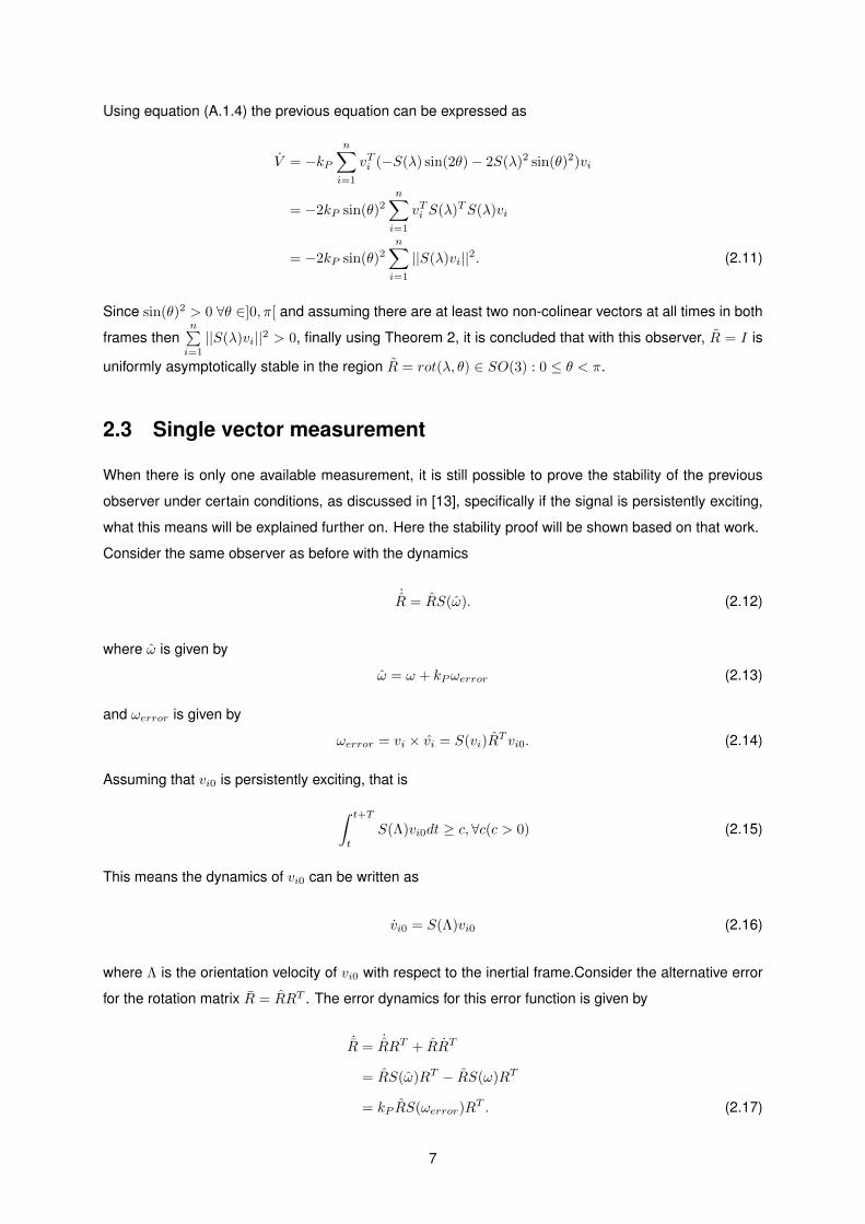
Using equation (A.1.4) the previous equation can be expressed as
V = −kPn∑i=1
vTi (−S(λ) sin(2θ)− 2S(λ)2 sin(θ)2)vi
= −2kP sin(θ)2n∑i=1
vTi S(λ)TS(λ)vi
= −2kP sin(θ)2n∑i=1
||S(λ)vi||2. (2.11)
Since sin(θ)2 > 0 ∀θ ∈]0, π[ and assuming there are at least two non-colinear vectors at all times in both
frames thenn∑i=1
||S(λ)vi||2 > 0, finally using Theorem 2, it is concluded that with this observer, R = I is
uniformly asymptotically stable in the region R = rot(λ, θ) ∈ SO(3) : 0 ≤ θ < π.
2.3 Single vector measurement
When there is only one available measurement, it is still possible to prove the stability of the previous
observer under certain conditions, as discussed in [13], specifically if the signal is persistently exciting,
what this means will be explained further on. Here the stability proof will be shown based on that work.
Consider the same observer as before with the dynamics
˙R = RS(ω). (2.12)
where ω is given by
ω = ω + kPωerror (2.13)
and ωerror is given by
ωerror = vi × vi = S(vi)RT vi0. (2.14)
Assuming that vi0 is persistently exciting, that is
∫ t+T
t
S(Λ)vi0dt ≥ c,∀c(c > 0) (2.15)
This means the dynamics of vi0 can be written as
vi0 = S(Λ)vi0 (2.16)
where Λ is the orientation velocity of vi0 with respect to the inertial frame.Consider the alternative error
for the rotation matrix R = RRT . The error dynamics for this error function is given by
˙R =˙RRT + RRT
= RS(ω)RT − RS(ω)RT
= kP RS(ωerror)RT . (2.17)
7
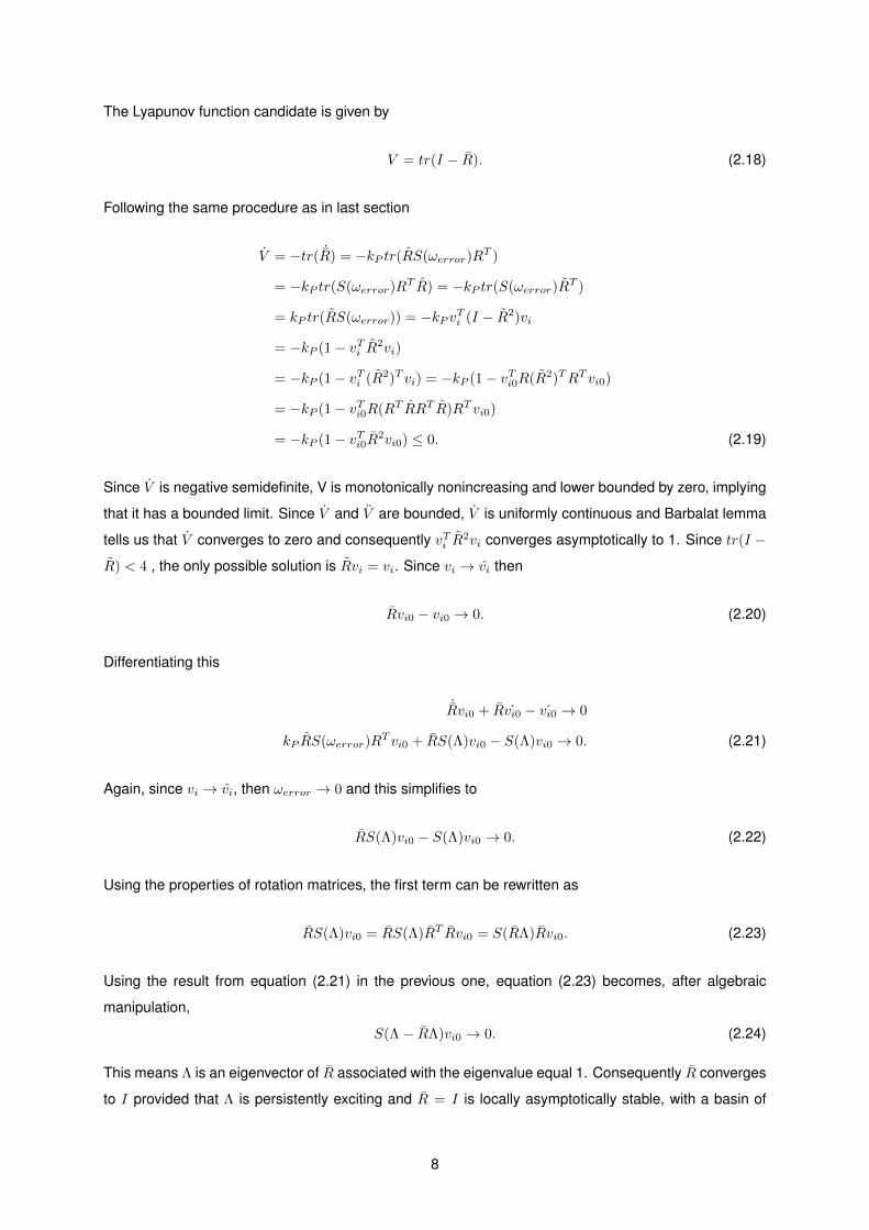
The Lyapunov function candidate is given by
V = tr(I − R). (2.18)
Following the same procedure as in last section
V = −tr( ˙R) = −kP tr(RS(ωerror)RT )
= −kP tr(S(ωerror)RT R) = −kP tr(S(ωerror)R
T )
= kP tr(RS(ωerror)) = −kP vTi (I − R2)vi
= −kP (1− vTi R2vi)
= −kP (1− vTi (R2)T vi) = −kP (1− vTi0R(R2)TRT vi0)
= −kP (1− vTi0R(RT RRT R)RT vi0)
= −kP (1− vTi0R2vi0) ≤ 0. (2.19)
Since V is negative semidefinite, V is monotonically nonincreasing and lower bounded by zero, implying
that it has a bounded limit. Since V and V are bounded, V is uniformly continuous and Barbalat lemma
tells us that V converges to zero and consequently vTi R2vi converges asymptotically to 1. Since tr(I −
R) < 4 , the only possible solution is Rvi = vi. Since vi → vi then
Rvi0 − vi0 → 0. (2.20)
Differentiating this
˙Rvi0 + R ˙vi0 − ˙vi0 → 0
kP RS(ωerror)RT vi0 + RS(Λ)vi0 − S(Λ)vi0 → 0. (2.21)
Again, since vi → vi, then ωerror → 0 and this simplifies to
RS(Λ)vi0 − S(Λ)vi0 → 0. (2.22)
Using the properties of rotation matrices, the first term can be rewritten as
RS(Λ)vi0 = RS(Λ)RT Rvi0 = S(RΛ)Rvi0. (2.23)
Using the result from equation (2.21) in the previous one, equation (2.23) becomes, after algebraic
manipulation,
S(Λ− RΛ)vi0 → 0. (2.24)
This means Λ is an eigenvector of R associated with the eigenvalue equal 1. Consequently R converges
to I provided that Λ is persistently exciting and R = I is locally asymptotically stable, with a basin of
8
attraction containing almost all initial conditions , i. e. all initial conditions such that tr(I − R) < 4. [13]
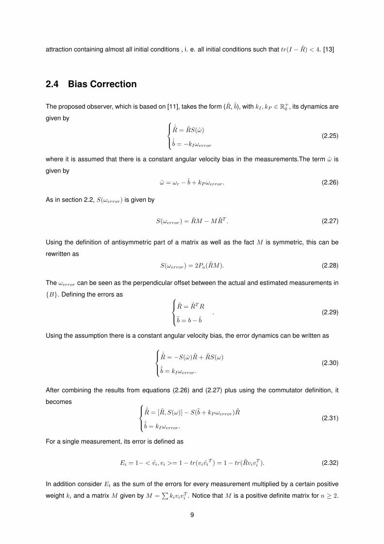
2.4 Bias Correction
The proposed observer, which is based on [11], takes the form (R, b), with kI , kP ∈ R+0 , its dynamics are
given by ˙R = RS(ω)
˙b = −kIωerror
(2.25)
where it is assumed that there is a constant angular velocity bias in the measurements.The term ω is
given by
ω = ωr − b+ kPωerror. (2.26)
As in section 2.2, S(ωerror) is given by
S(ωerror) = RM −MRT . (2.27)
Using the definition of antisymmetric part of a matrix as well as the fact M is symmetric, this can be
rewritten as
S(ωerror) = 2Pa(RM). (2.28)
The ωerror can be seen as the perpendicular offset between the actual and estimated measurements in
{B}. Defining the errors as R = RTR
b = b− b. (2.29)
Using the assumption there is a constant angular velocity bias, the error dynamics can be written as
˙R = −S(ω)R+ RS(ω)
˙b = kIωerror.
(2.30)
After combining the results from equations (2.26) and (2.27) plus using the commutator definition, it
becomes ˙R = [R, S(ω)]− S(b+ kPωerror)R
˙b = kIωerror.
(2.31)
For a single measurement, its error is defined as
Ei = 1− < vi, vi >= 1− tr(viviT ) = 1− tr(RvivTi ). (2.32)
In addition consider Et as the sum of the errors for every measurement multiplied by a certain positive
weight ki and a matrix M given by M =∑kiviv
Ti . Notice that M is a positive definite matrix for n ≥ 2.
9
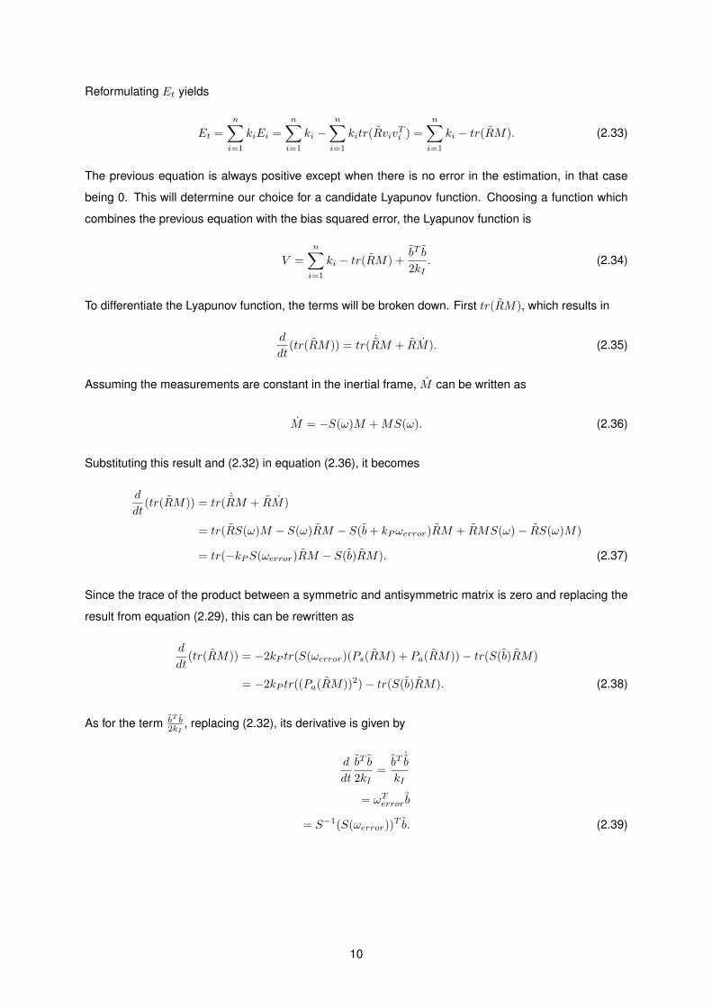
Reformulating Et yields
Et =
n∑i=1
kiEi =
n∑i=1
ki −n∑i=1
kitr(RvivTi ) =
n∑i=1
ki − tr(RM). (2.33)
The previous equation is always positive except when there is no error in the estimation, in that case
being 0. This will determine our choice for a candidate Lyapunov function. Choosing a function which
combines the previous equation with the bias squared error, the Lyapunov function is
V =
n∑i=1
ki − tr(RM) +bT b
2kI. (2.34)
To differentiate the Lyapunov function, the terms will be broken down. First tr(RM), which results in
d
dt(tr(RM)) = tr( ˙RM + RM). (2.35)
Assuming the measurements are constant in the inertial frame, M can be written as
M = −S(ω)M +MS(ω). (2.36)
Substituting this result and (2.32) in equation (2.36), it becomes
d
dt(tr(RM)) = tr( ˙RM + RM)
= tr(RS(ω)M − S(ω)RM − S(b+ kPωerror)RM + RMS(ω)− RS(ω)M)
= tr(−kPS(ωerror)RM − S(b)RM). (2.37)
Since the trace of the product between a symmetric and antisymmetric matrix is zero and replacing the
result from equation (2.29), this can be rewritten as
d
dt(tr(RM)) = −2kP tr(S(ωerror)(Ps(RM) + Pa(RM))− tr(S(b)RM)
= −2kP tr((Pa(RM))2)− tr(S(b)RM). (2.38)
As for the term bT b2kI
, replacing (2.32), its derivative is given by
d
dt
bT b
2kI=bT
˙b
kI
= ωTerror b
= S−1(S(ωerror))T b. (2.39)
10
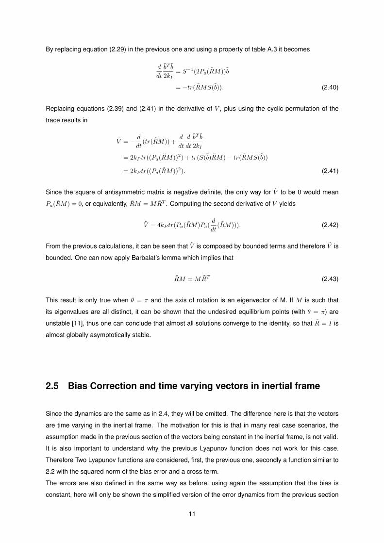
By replacing equation (2.29) in the previous one and using a property of table A.3 it becomes
d
dt
bT b
2kI= S−1(2Pa(RM))b
= −tr(RMS(b)). (2.40)
Replacing equations (2.39) and (2.41) in the derivative of V , plus using the cyclic permutation of the
trace results in
V = − d
dt(tr(RM)) +
d
dt
d
dt
bT b
2kI
= 2kP tr((Pa(RM))2) + tr(S(b)RM)− tr(RMS(b))
= 2kP tr((Pa(RM))2). (2.41)
Since the square of antisymmetric matrix is negative definite, the only way for V to be 0 would mean
Pa(RM) = 0, or equivalently, RM = MRT . Computing the second derivative of V yields
V = 4kP tr(Pa(RM)Pa(d
dt(RM))). (2.42)
From the previous calculations, it can be seen that V is composed by bounded terms and therefore V is
bounded. One can now apply Barbalat’s lemma which implies that
RM = MRT (2.43)
This result is only true when θ = π and the axis of rotation is an eigenvector of M. If M is such that
its eigenvalues are all distinct, it can be shown that the undesired equilibrium points (with θ = π) are
unstable [11], thus one can conclude that almost all solutions converge to the identity, so that R = I is
almost globally asymptotically stable.
2.5 Bias Correction and time varying vectors in inertial frame
Since the dynamics are the same as in 2.4, they will be omitted. The difference here is that the vectors
are time varying in the inertial frame. The motivation for this is that in many real case scenarios, the
assumption made in the previous section of the vectors being constant in the inertial frame, is not valid.
It is also important to understand why the previous Lyapunov function does not work for this case.
Therefore Two Lyapunov functions are considered, first, the previous one, secondly a function similar to
2.2 with the squared norm of the bias error and a cross term.
The errors are also defined in the same way as before, using again the assumption that the bias is
constant, here will only be shown the simplified version of the error dynamics from the previous section
11
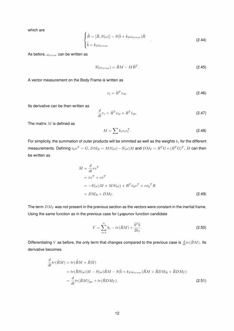
which are ˙R = [R, S(ω)]− S(b+ kPωerror)R
˙b = kIωerror
. (2.44)
As before, ωerror can be written as
S(ωerror) = RM −MRT . (2.45)
A vector measurement on the Body Frame is written as
vi = RT vi0. (2.46)
Its derivative can be then written asd
dtvi = RT vi0 +RT vi0. (2.47)
The matrix M is defined as
M =∑
kivivTi . (2.48)
For simplicity, the summation of outer products will be ommited as well as the weights ki for the different
measurements. Defining v0vT = G, DMR = MS(ω)−S(ω)M and DMT = RTG+(RTG)T , M can then
be written as
M =d
dtvvT
= vvT + vvT
= −S(ω)M +MS(ω) +RT v0vT + vv0
TR
= DMR +DMT . (2.49)
The term DMT was not present in the previous section as the vectors were constant in the inertial frame.
Using the same function as in the previous case for Lyapunov function candidate
V =
n∑i=1
ki − tr(RM) +bT b
2kI. (2.50)
Differentiating V as before, the only term that changes compared to the previous case is ddt tr(RM). Its
derivative becomes
d
dttr(RM) = tr( ˙RM + RM)
= tr(RS(ω)M − S(ω)RM − S(b+ kPωerror)RM + RDMR + RDMT )
=d
dttr(RM)|pc + tr(RDMT ). (2.51)
12
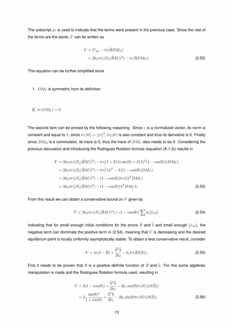
The subscript pc is used to indicate that the terms were present in the previous case. Since the rest of
the terms are the same, V can be written as
V = V |pc − tr(RDMT )
= 2kP tr((Pa(RM))2)− tr(RDMT ). (2.52)
This equation can be further simplified since
1. DMT is symmetric from its definition
2. tr(DMT ) = 0
The second item can be proved by the following reasoning. Since v is a normalized vector, its norm is
constant and equal to 1, since tr(M) = ||v||2, tr(M) is also constant and thus its derivative is 0. Finally
since DMR is a commutator, its trace is 0, thus the trace of DMT also needs to be 0. Considering the
previous discussion and introducing the Rodrigues Rotation formula (equation (A.1.3)) results in
V = 2kP tr((Pa(RM))2)− tr((I + S(λ) sin(θ) + S(λ)2(1− cos(θ)))DMT )
= 2kP tr((Pa(RM))2)− tr((λλT − I)(1− cos(θ))DMT )
= 2kP tr((Pa(RM))2)− (1− cos(θ))tr(λλTDMT )
= 2kP tr((Pa(RM))2)− (1− cos(θ))λTDMTλ. (2.53)
From this result we can obtain a conservative bound on V given by
V ≤ 2kP tr((Pa(RM))2) + (1− cos(θ))∑
ki‖vi0‖ (2.54)
indicating that for small enough initial conditions for the errors R and b and small enough ‖vi0‖, the
negative term can dominate the positive term in (2.54), meaning that V is decreasing and the desired
equilibrium point is locally uniformly asymptotically stable. To obtain a less conservative result, consider
V = tr(I − R) +bT b
2kI− kctr(RS(b)). (2.55)
First it needs to be proven that V is a positive definite function of R and b. For this some algebraic
manipulation is made and the Rodrigues Rotation formula used, resulting in
V = 2(1− cos(θ)) +bT b
2kI− 2kc sin(θ)tr(S(λ)S(b))
= 2sin(θ)2
1 + cos(θ)+bT b
2kI− 2kc sin(θ)tr(S(λ)S(b)). (2.56)
13
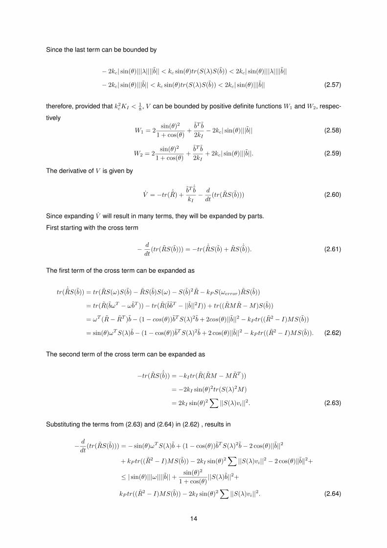
Since the last term can be bounded by
− 2kc| sin(θ)|||λ||||b|| < kc sin(θ)tr(S(λ)S(b)) < 2kc| sin(θ)|||λ||||b||
− 2kc| sin(θ)|||b|| < kc sin(θ)tr(S(λ)S(b)) < 2kc| sin(θ)|||b|| (2.57)
therefore, provided that k2cKI <18 , V can be bounded by positive definite functions W1 and W2, respec-
tively
W1 = 2sin(θ)2
1 + cos(θ)+bT b
2kI− 2kc| sin(θ)|||b|| (2.58)
W2 = 2sin(θ)2
1 + cos(θ)+bT b
2kI+ 2kc| sin(θ)|||b||. (2.59)
The derivative of V is given by
V = −tr( ˙R) +bT
˙b
kI− d
dt(tr(RS(b))) (2.60)
Since expanding V will result in many terms, they will be expanded by parts.
First starting with the cross term
− d
dt(tr(RS(b))) = −tr( ˙RS(b) + RS(
˙b)). (2.61)
The first term of the cross term can be expanded as
tr( ˙RS(b)) = tr(RS(ω)S(b)− RS(b)S(ω)− S(b)2R− kPS(ωerror)RS(b))
= tr(R(bωT − ωbT ))− tr(R(bbT − ||b||2I)) + tr((RMR−M)S(b))
= ωT (R− RT )b− (1− cos(θ))bTS(λ)2b+ 2cos(θ)||b||2 − kP tr((R2 − I)MS(b))
= sin(θ)ωTS(λ)b− (1− cos(θ))bTS(λ)2b+ 2 cos(θ)||b||2 − kP tr((R2 − I)MS(b)). (2.62)
The second term of the cross term can be expanded as
−tr(RS(˙b)) = −kItr(R(RM −MRT ))
= −2kI sin(θ)2tr(S(λ)2M)
= 2kI sin(θ)2∑||S(λ)vi||2. (2.63)
Substituting the terms from (2.63) and (2.64) in (2.62) , results in
− d
dt(tr(RS(b))) = − sin(θ)ωTS(λ)b+ (1− cos(θ))bTS(λ)2b− 2 cos(θ)||b||2
+ kP tr((R2 − I)MS(b))− 2kI sin(θ)2
∑||S(λ)vi||2 − 2 cos(θ)‖b‖2+
≤ | sin(θ)|||ω||||b||+ sin(θ)2
1 + cos(θ)||S(λ)b||2+
kP tr((R2 − I)MS(b))− 2kI sin(θ)2
∑||S(λ)vi||2. (2.64)
14
The term kP tr((R2 − I)MS(b)) can be bounded by1
kP tr((R2 − I)MS(b)) ≤ S−1(2Pa((R2 − I)M))T b
≤ ||S−1(2Pa(R2M))||||b||
≤√
2||(I − R2)M ||||b||
≤√
2||I − R2||||M ||||b||
= 4 sin(θ)||M ||||b||. (2.65)
Substituting the previous result in the bound for − ddt (tr(RS(b))), plus considering θ ∈]0, π2 [
− d
dt(tr(RS(b))) ≤ | sin(θ)|||ω||||b||+sin(θ)2(
1
2||S(λ)b||2−2kI
∑||S(λ)vi||2)+4 sin(θ)||M ||||b||−2kc cos(θ)‖b‖2.
(2.66)
Regarding the term˙bT b2kI
from the bias term, it can be written as
˙bT b
2kI= S−1(2Pa(RM))T b. (2.67)
This term can then be bounded by
˙bT b
2kI≤ ||S−1(2Pa(RM))||||b||
= ||S−1(2Pa((R− I)M))||||b||
≤√
2||(I − R)M ||||b||
≤ 2||M || sin(θ)||b||. (2.68)
In the previous steps, the properties of table A.2 were used for the inequalities. The term tr( ˙R) can be
written as
tr( ˙R) = 2kP sin(θ)2n∑i=1
vTi S(λ)2vi − tr(RS(b))
= 2kP sin(θ)2n∑i=1
vTi ||S(λ)vi||2 − tr(RS(b))
≤ 2kP sin(θ)2n∑i=1
vTi ||S(λ)vi||2 + 2 sin(θ)||b||. (2.69)
Collecting all the terms from 2.70, 2.69 and 2.65, one can define the system
V ≤ −[| sin(θ)| ||b||
]a11 a12
a12 a22
| sin(θ)|
||b||
(2.70)
1||I − R|| = 2√2 sin(θ)
15
where Bω is a bound for ||ω|| and a11,a12,a22 are given by
a11 = 2(kP − kckI)
∑||S(λ)vi||2 + kc
1+cos(θ) ||S(λ)b||2
a12 = −(2kc||M ||+ ||M ||+ 1 + kcBω
2 )
a22 = 2kc cos(θ)
. (2.71)
To make the matrix negative definite
a11 > 0
a11a22 − a212 > 0
. (2.72)
This translates in setting up the gains kP , kI and the constant kc. By obeying this conditions, uniform
asymptotic stability of the observer errors can be guaranteed, using Theorem 1. Since for this stability
proof θ needed to be less than π2 , the domain is smaller than for the previous section case, nonetheless,
the simulation results suggest that the observer can perform very well in the presence of angular velocity
bias, even over a larger interval. This may as well be just a problem of finding a better Lyapunov function.
Important note: Although one is restricting only to θ < π2 , this also imposes a restriction on b.
2.6 Simulation Results
In this section the cases from the previous sections are simulated for situations where they are applica-
ble. In all examples, θ is the angle of the rotation matrix error in the angle axis representation.
Example 1 Simple case
A Simulink Model is created and tested, in which a system of differential equations to simulate R is
used in order to have the vectors in both reference frames, which are needed to feed the observer
system.
The vectors are time varying on the inertial frame and the angular velocity input is driven by
ω = 3 sin(150t)[1 1 1
]T. (2.73)
The vectors on the Inertial Frame were created as an arbitrary matrix driven by sinusoidal functions
and its column vectors were normalized.
For initial conditions one assumed the Estimate to be
R0 =
0.7071 0.6124 0.3536
0 0.5000 −0.8660
−0.7071 0.6124 0.3536
(2.74)
16
the initial rotation as
R0 =
0.4698 −0.3420 0.8138
0.1710 0.9397 0.2962
−0.8660 0 0.5000
. (2.75)
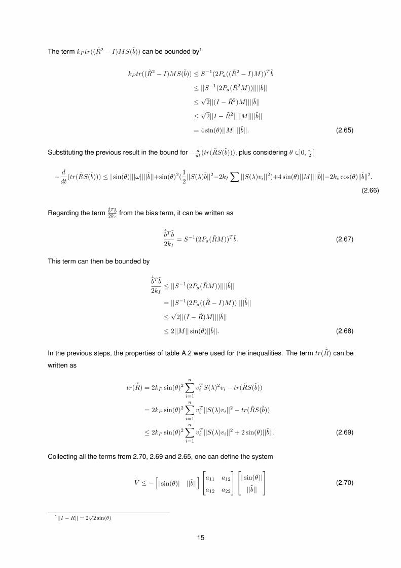
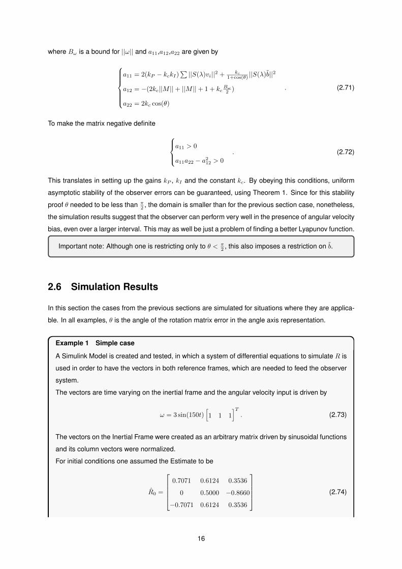
This choice was made in order to have θ < π2 . The constant kP was defined as kP = 1. Figure
2.1 shows the Simulink representation of the system , where the inputs are in yellow, the observer
system is light blue, the system is dark blue and the Lyapunov function is white. Figure 2.4 shows
the response obtained for the Lyapunov function. It can be seen that the error goes to zero just
after 2 seconds, crosschecking its derivative it can be seen that its value is always less than 0, thus
in agreement with the conditions for the stability proof.
Figure 2.1: The Simulink model of the System.
Figure 2.2: Lyapunov function for initial θ <π2
Figure 2.3: Lyapunov function derivative for
initial θ < π2
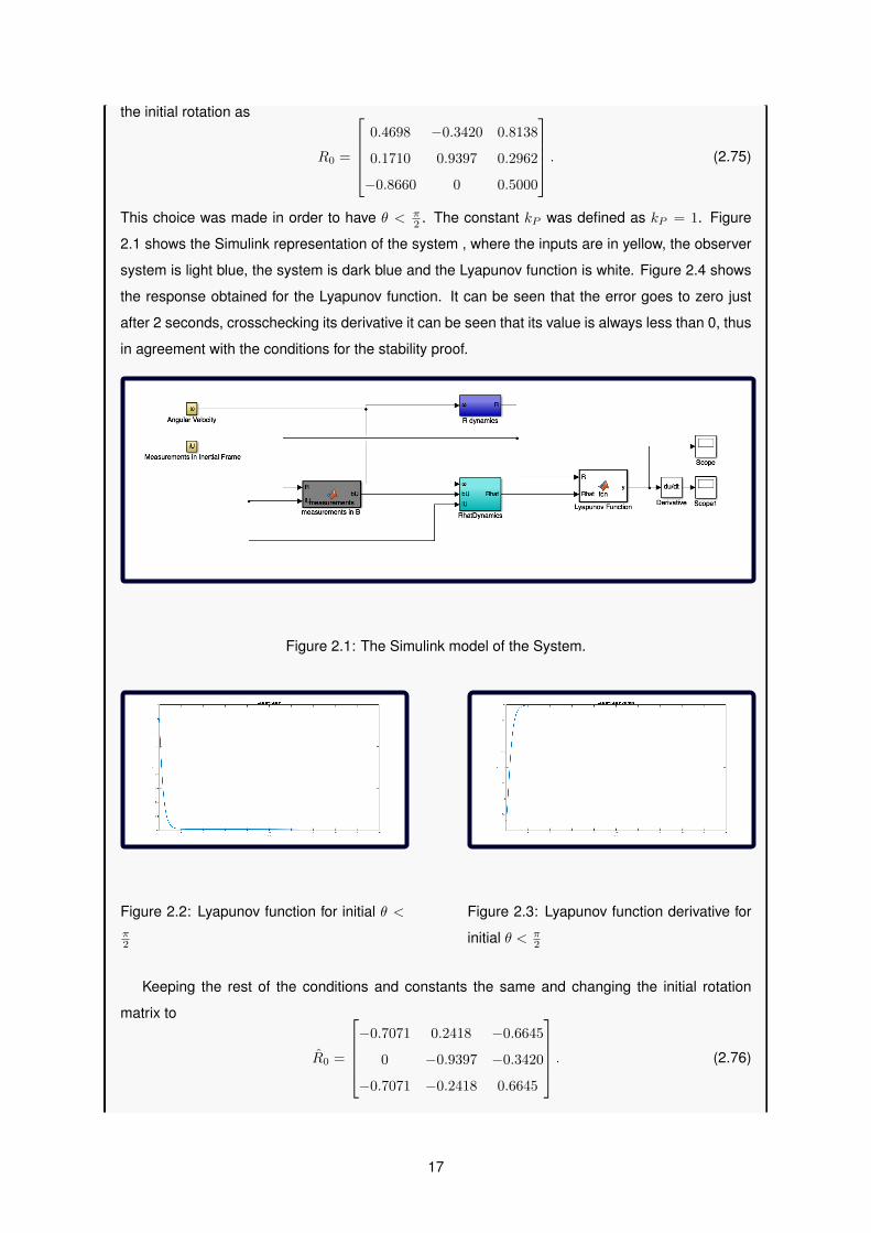
Keeping the rest of the conditions and constants the same and changing the initial rotation
matrix to
R0 =
−0.7071 0.2418 −0.6645
0 −0.9397 −0.3420
−0.7071 −0.2418 0.6645
. (2.76)
17
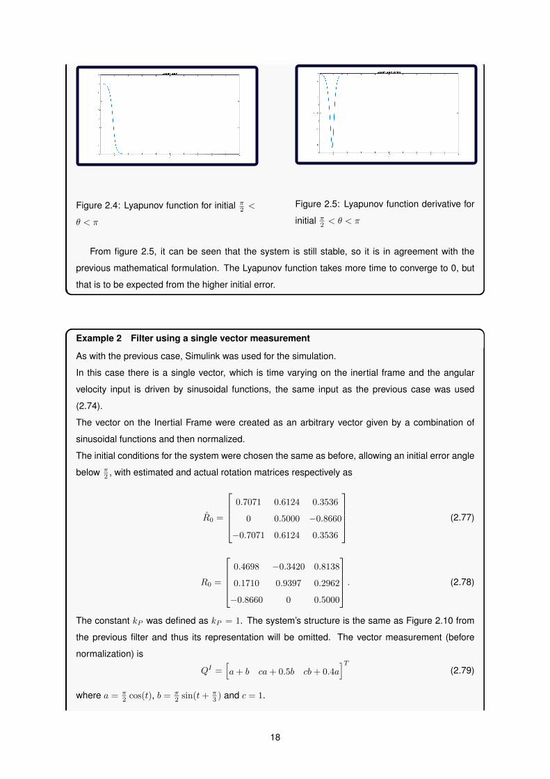
Figure 2.4: Lyapunov function for initial π2 <
θ < π
Figure 2.5: Lyapunov function derivative for
initial π2 < θ < π
From figure 2.5, it can be seen that the system is still stable, so it is in agreement with the
previous mathematical formulation. The Lyapunov function takes more time to converge to 0, but
that is to be expected from the higher initial error.
Example 2 Filter using a single vector measurement
As with the previous case, Simulink was used for the simulation.
In this case there is a single vector, which is time varying on the inertial frame and the angular
velocity input is driven by sinusoidal functions, the same input as the previous case was used
(2.74).
The vector on the Inertial Frame were created as an arbitrary vector given by a combination of
sinusoidal functions and then normalized.
The initial conditions for the system were chosen the same as before, allowing an initial error angle
below π2 , with estimated and actual rotation matrices respectively as
R0 =
0.7071 0.6124 0.3536
0 0.5000 −0.8660
−0.7071 0.6124 0.3536
(2.77)
R0 =
0.4698 −0.3420 0.8138
0.1710 0.9397 0.2962
−0.8660 0 0.5000
. (2.78)
The constant kP was defined as kP = 1. The system’s structure is the same as Figure 2.10 from
the previous filter and thus its representation will be omitted. The vector measurement (before
normalization) is
QI =[a+ b ca+ 0.5b cb+ 0.4a
]T(2.79)
where a = π2 cos(t), b = π
2 sin(t+ π3 ) and c = 1.
18
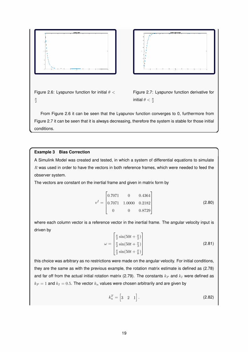
Figure 2.6: Lyapunov function for initial θ <π2
Figure 2.7: Lyapunov function derivative for
initial θ < π2
From Figure 2.6 it can be seen that the Lyapunov function converges to 0, furthermore from
Figure 2.7 it can be seen that it is always decreasing, therefore the system is stable for those initial
conditions.
Example 3 Bias Correction
A Simulink Model was created and tested, in which a system of differential equations to simulate
R was used in order to have the vectors in both reference frames, which were needed to feed the
observer system.
The vectors are constant on the inertial frame and given in matrix form by
vI =
0.7071 0 0.4364
0.7071 1.0000 0.2182
0 0 0.8729
(2.80)
where each column vector is a reference vector in the inertial frame. The angular velocity input is
driven by
ω =
π2 sin(50t+ π
2 )
π2 sin(50t+ π
3 )
π2 sin(50t+ π
8 )
(2.81)
this choice was arbitrary as no restrictions were made on the angular velocity. For initial conditions,
they are the same as with the previous example, the rotation matrix estimate is defined as (2.78)
and far off from the actual initial rotation matrix (2.79). The constants kP and kI were defined as
kP = 1 and kI = 0.5. The vector kn values were chosen arbitrarily and are given by
kTn =[3 2 1
]. (2.82)
19
The initial bias estimate was assumed as
bT0 =[2 2 2
]. (2.83)
The actual bias is given by
bT0 =[1 1 1
](2.84)
this choice again is purely arbitrary, furthermore these values would be quite high for a real situa-
tion. The Simulink representation of the system is shown in figure 2.10, where the inputs to system,
are in yellow, the constants used for the system are in magenta, the Observer System is light blue,
the System is dark blue. The red block is for the calculation of the errors and the orange blocks
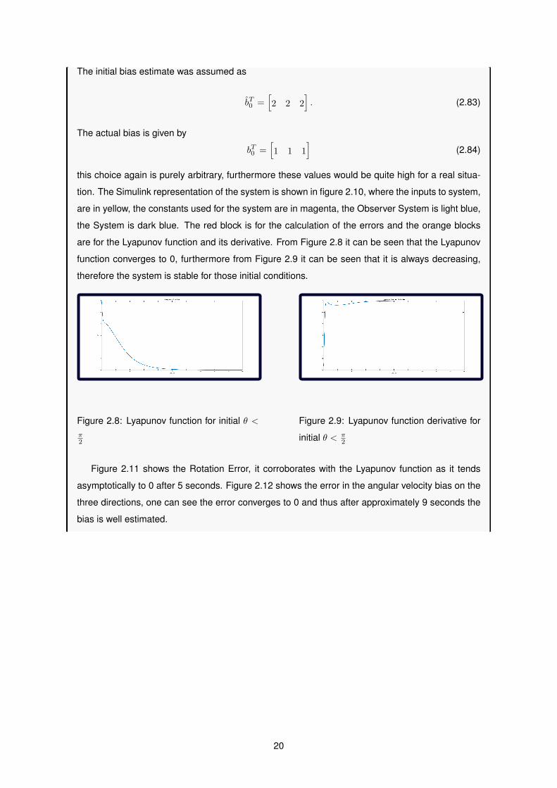
are for the Lyapunov function and its derivative. From Figure 2.8 it can be seen that the Lyapunov
function converges to 0, furthermore from Figure 2.9 it can be seen that it is always decreasing,
therefore the system is stable for those initial conditions.
Figure 2.8: Lyapunov function for initial θ <π2
Figure 2.9: Lyapunov function derivative for
initial θ < π2
Figure 2.11 shows the Rotation Error, it corroborates with the Lyapunov function as it tends
asymptotically to 0 after 5 seconds. Figure 2.12 shows the error in the angular velocity bias on the
three directions, one can see the error converges to 0 and thus after approximately 9 seconds the
bias is well estimated.
20
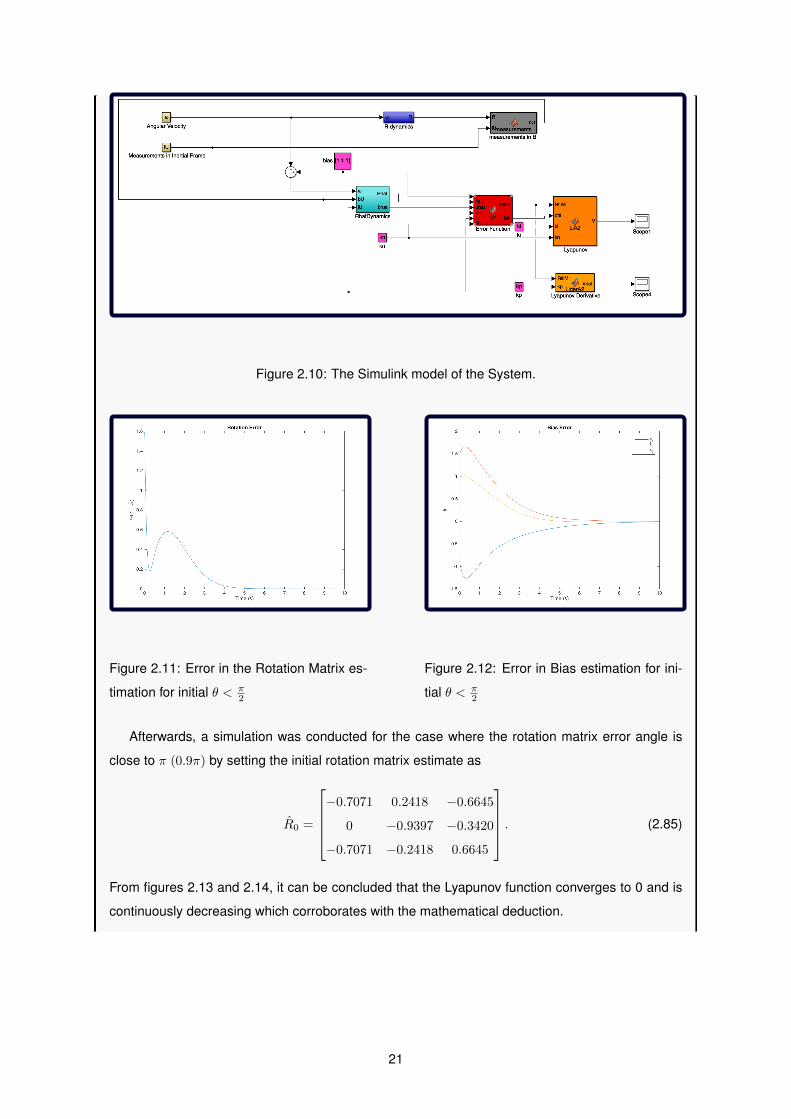
Figure 2.10: The Simulink model of the System.
Figure 2.11: Error in the Rotation Matrix es-
timation for initial θ < π2
Figure 2.12: Error in Bias estimation for ini-
tial θ < π2
Afterwards, a simulation was conducted for the case where the rotation matrix error angle is
close to π (0.9π) by setting the initial rotation matrix estimate as
R0 =
−0.7071 0.2418 −0.6645
0 −0.9397 −0.3420
−0.7071 −0.2418 0.6645
. (2.85)
From figures 2.13 and 2.14, it can be concluded that the Lyapunov function converges to 0 and is
continuously decreasing which corroborates with the mathematical deduction.
21
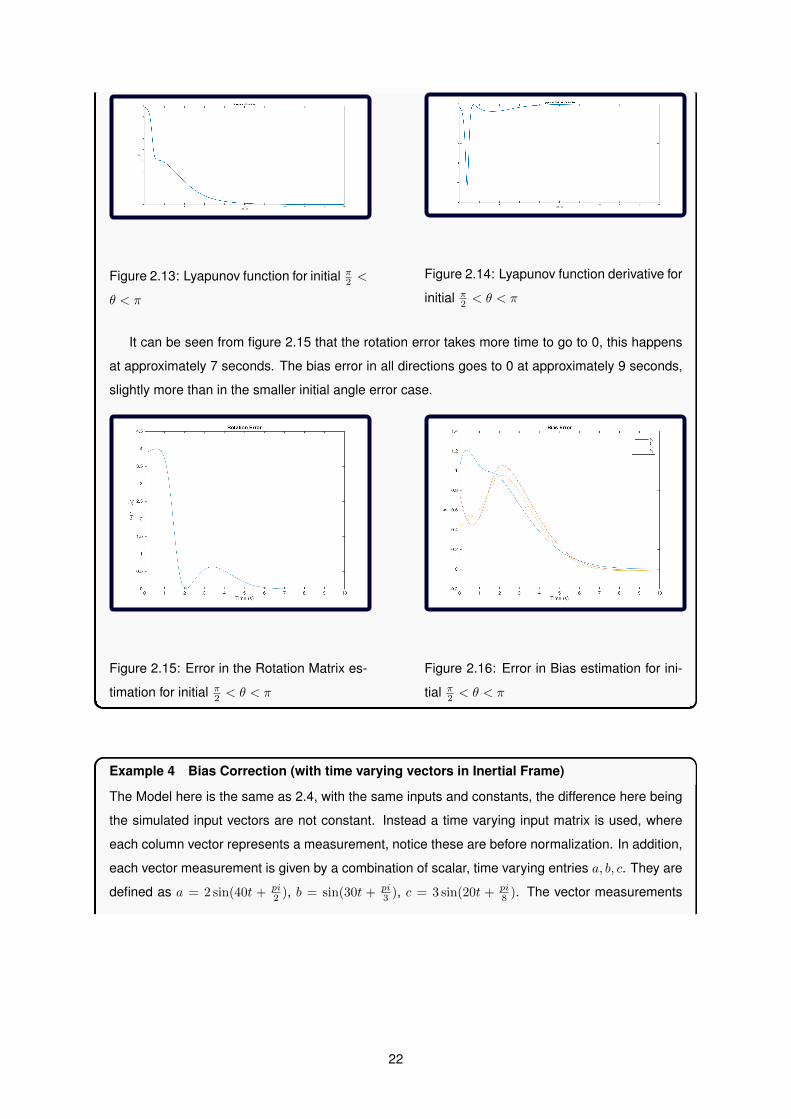
Figure 2.13: Lyapunov function for initial π2 <
θ < π
Figure 2.14: Lyapunov function derivative for
initial π2 < θ < π
It can be seen from figure 2.15 that the rotation error takes more time to go to 0, this happens
at approximately 7 seconds. The bias error in all directions goes to 0 at approximately 9 seconds,
slightly more than in the smaller initial angle error case.
Figure 2.15: Error in the Rotation Matrix es-
timation for initial π2 < θ < π
Figure 2.16: Error in Bias estimation for ini-
tial π2 < θ < π
Example 4 Bias Correction (with time varying vectors in Inertial Frame)
The Model here is the same as 2.4, with the same inputs and constants, the difference here being
the simulated input vectors are not constant. Instead a time varying input matrix is used, where
each column vector represents a measurement, notice these are before normalization. In addition,
each vector measurement is given by a combination of scalar, time varying entries a, b, c. They are
defined as a = 2 sin(40t + pi2 ), b = sin(30t + pi
3 ), c = 3 sin(20t + pi8 ). The vector measurements
22

matrix before normalization is given by
QI =
−abc b+ a b+ c
b c a
a b c
. (2.86)
The initial rotation error is chosen as lower than π2 , since this was the restriction on the stability
proof. The angular velocity input is driven by
ω =
π2 sin(50t+ π
2 )
π2 sin(50t+ π
3 )
π2 sin(50t+ π
8 )
(2.87)
here the angular velocity was kept as a bounded value in order to satisfy the assumption in the
proof. For the rest of the initial conditions, they are the same ones as the ones from the previous
example for the θ < π2 case.
The Lyapunov function used is the second one, whose stability was proven for θ < π2 . From figures
2.17 and 2.18 it can be seen that the Lyapunov function converges to 0 and is always decreasing,
agreeing with the proof.
Figure 2.17: Lyapunov function for initial θ <
π2
Figure 2.18: Lyapunov function derivative for
initial θ < π2
By changing the rotation matrix estimation to
R0 =
−0.7071 0.2418 −0.6645
0 −0.9397 −0.3420
−0.7071 −0.2418 0.6645
, (2.88)
from Figure 2.19 one can see that the Rotation Matrix error converges to 0 as well, the differ-
ence with the previous case is some shakiness between 0.2 and 3 seconds. The error bias also
converges to 0 on the three directions as one can see from figure 2.20, this happens as with the
previous case approximately 9 seconds later.
These results suggest that for θ < π2 the behaviour is quite similar to the constant measurement
23
case.
Figure 2.19: Error in the Rotation Matrix es-
timation for initial θ < π2
Figure 2.20: Error in Bias estimation for ini-
tial θ < π2
Changing the initial rotation matrix estimate to
R0 =
−0.7071 0.2418 −0.6645
0 −0.9397 −0.3420
−0.7071 −0.2418 0.6645
(2.89)
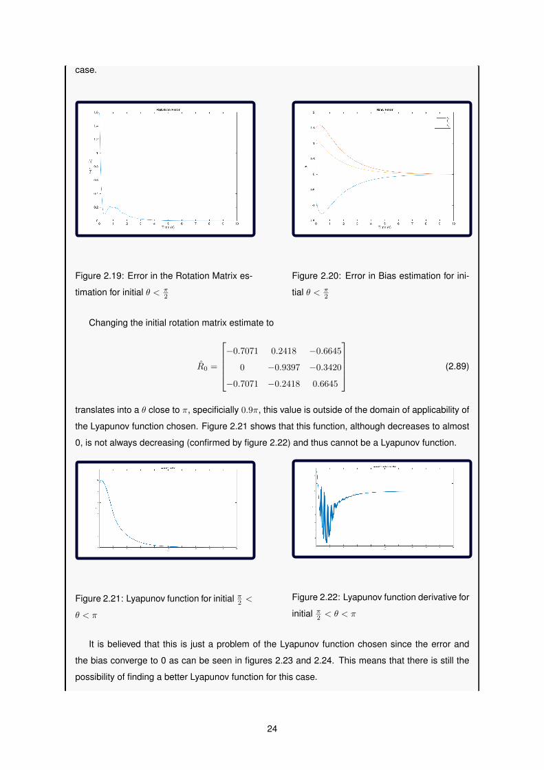
translates into a θ close to π, specificially 0.9π, this value is outside of the domain of applicability of
the Lyapunov function chosen. Figure 2.21 shows that this function, although decreases to almost
0, is not always decreasing (confirmed by figure 2.22) and thus cannot be a Lyapunov function.
Figure 2.21: Lyapunov function for initial π2 <
θ < π
Figure 2.22: Lyapunov function derivative for
initial π2 < θ < π
It is believed that this is just a problem of the Lyapunov function chosen since the error and
the bias converge to 0 as can be seen in figures 2.23 and 2.24. This means that there is still the
possibility of finding a better Lyapunov function for this case.
24
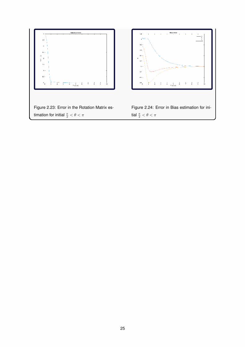
Figure 2.23: Error in the Rotation Matrix es-
timation for initial π2 < θ < π
Figure 2.24: Error in Bias estimation for ini-
tial π2 < θ < π
25
Chapter 3
Attitude Estimation Results
3.1 Experimental setup
In order to test the observers using vector measurements, the existing platforms and sensors available
in DSOR/ISR were used, specifically a quadcopter equipped with a Hokuyo LiDAR, building on the work
of [20].
This LiDAR measures 1081 distances corresponding to the angles between −135◦ and 135◦ . The vehi-
cle’s LiDAR will hit one or two faces of the cuboid shaped object, depending on its orientation, and the
intersection between them will result in one or two straight lines, which from here on will be called edges
to follow the terminology of [20]. The edges are represented by a matrix QB , expressed in {B}, where
each column of this matrix represents an edge and expressed in {I} by the matrix QI , noticing that the
projection in the XY plane of this reference frame corresponds to the section of the pier. Throughout this
simulation the column vectors are normalized (vi = Qi
‖Qi‖ ) in order to have a problem in the form [21].
Notice however, that due to the geometry of the problem, it is possible that in some cases the vehicle’s
facing only one side of the pier and thus has only one vector measurement, in this case, while the sys-
tem would still converge, this convergence would take more time as previously discussed.
Two blocks are used for the conversion of between the LiDAR distances measured and the vectors
needed for the observer, which were already developed at DSOR prior to this work. One block is re-
sponsible for clustering the data points and selects the one whose centroid is the closest from the origin
in {B} . For the second block, after receiving the clustered data points, it estimates the dimensions of
the pier, removes the outliers and calculates the edges. Estimating the dimensions of the pier is the main
difference with respect with [20], which relied heavily on knowing beforehand the edge dimensions. The
second block requires as input, besides the cluster information (number of points, distances,angles), the
absolute height at which the Quadcopter is. To obtain this information, it can be used, for example, the
barometer data. However, sometimes the barometer information is unreliable, so an approximate height
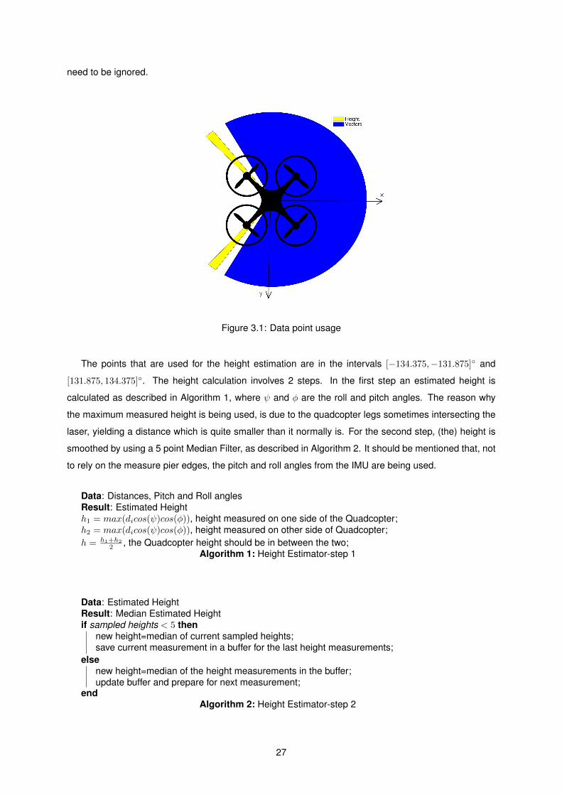
is obtained by equipping the Quadcopter with mirrors which reflect the LiDAR rays into the ground. Fig-
ure 3.1 shows the correspondence between the data points and their usage, due to using some laser
points for the height estimation, some points inbetween the height estimation and the edges calculation
26
need to be ignored.
Figure 3.1: Data point usage
The points that are used for the height estimation are in the intervals [−134.375,−131.875]◦ and
[131.875, 134.375]◦. The height calculation involves 2 steps. In the first step an estimated height is
calculated as described in Algorithm 1, where ψ and φ are the roll and pitch angles. The reason why
the maximum measured height is being used, is due to the quadcopter legs sometimes intersecting the
laser, yielding a distance which is quite smaller than it normally is. For the second step, (the) height is
smoothed by using a 5 point Median Filter, as described in Algorithm 2. It should be mentioned that, not
to rely on the measure pier edges, the pitch and roll angles from the IMU are being used.
Data: Distances, Pitch and Roll anglesResult: Estimated Heighth1 = max(dicos(ψ)cos(φ)), height measured on one side of the Quadcopter;h2 = max(dicos(ψ)cos(φ)), height measured on other side of Quadcopter;h = h1+h2
2 , the Quadcopter height should be in between the two;Algorithm 1: Height Estimator-step 1
Data: Estimated HeightResult: Median Estimated Heightif sampled heights < 5 then
new height=median of current sampled heights;save current measurement in a buffer for the last height measurements;
elsenew height=median of the height measurements in the buffer;update buffer and prepare for next measurement;
endAlgorithm 2: Height Estimator-step 2
27
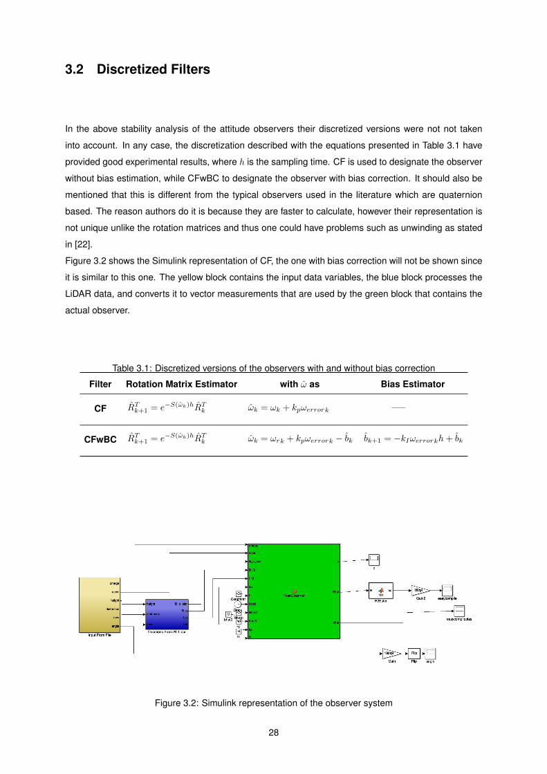
3.2 Discretized Filters
In the above stability analysis of the attitude observers their discretized versions were not not taken
into account. In any case, the discretization described with the equations presented in Table 3.1 have
provided good experimental results, where h is the sampling time. CF is used to designate the observer
without bias estimation, while CFwBC to designate the observer with bias correction. It should also be
mentioned that this is different from the typical observers used in the literature which are quaternion
based. The reason authors do it is because they are faster to calculate, however their representation is
not unique unlike the rotation matrices and thus one could have problems such as unwinding as stated
in [22].
Figure 3.2 shows the Simulink representation of CF, the one with bias correction will not be shown since
it is similar to this one. The yellow block contains the input data variables, the blue block processes the
LiDAR data, and converts it to vector measurements that are used by the green block that contains the
actual observer.
Table 3.1: Discretized versions of the observers with and without bias correction
Filter Rotation Matrix Estimator with ω as Bias Estimator
CF RTk+1 = e−S(ωk)hRTk ωk = ωk + kpωerrork –––
CFwBC RTk+1 = e−S(ωk)hRTk ωk = ωrk + kpωerrork − bk bk+1 = −kIωerrorkh+ bk
Figure 3.2: Simulink representation of the observer system
28

Data: Vector Measurements, Angular velocity
Result: Estimated Rotation Matrix
if Simulation Starts then
Initialize next estimates;
else
current estimate is the previous next estimate;
Normalize measurements;
Calculate ωerror ;
Calculate next estimates;
endAlgorithm 3: Pose Observer pseudo code
3.3 LiDAR sensor Simulation
Before testing the observers with real data, a simulink block was created to simulate the sensor data
which is obtained from the LiDAR.
Data: Rotation Matrix, Pier Position in I, Quadcopter Position in I, dimensions of Pier
Result: distance vectora, new, altitude
Initialize Pier vertices in I;
Rotate the Pier vertices to B;
Determine the vertices that define the cross section of the Pier in B;
Define the edges made of the vertices; for range of angles of the LiDAR do
for range of edges of the pier do
if nth edge of pier and the ith laser angle intersect thenCalculate intersection between the edge of the pier and the ith laser angle;
Calculate distance from the intersection to the origin (aux);
ith distance is equal to the mininum between aux and ith distanceb;
end
end
end
if distance vector is equal to the previous distance vector thennew=0;
elsenew=1;
endAlgorithm 4: LiDAR Sensor Block
avector with 1081 distancesbFor distances bigger than 0
The Simulink block created needs as input the rotation matrix from {I} to {B}, the position of the
29
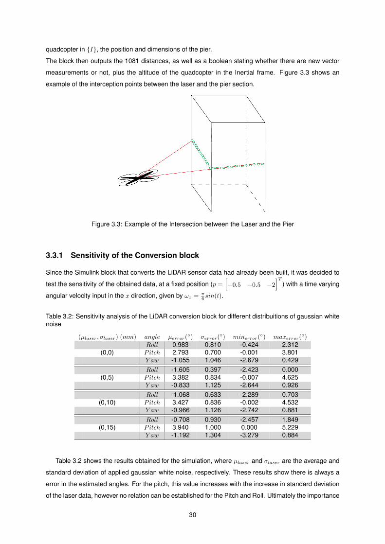
quadcopter in {I}, the position and dimensions of the pier.
The block then outputs the 1081 distances, as well as a boolean stating whether there are new vector
measurements or not, plus the altitude of the quadcopter in the Inertial frame. Figure 3.3 shows an
example of the interception points between the laser and the pier section.
Figure 3.3: Example of the Intersection between the Laser and the Pier
3.3.1 Sensitivity of the Conversion block
Since the Simulink block that converts the LiDAR sensor data had already been built, it was decided to
test the sensitivity of the obtained data, at a fixed position (p =[−0.5 −0.5 −2
]T) with a time varying
angular velocity input in the x direction, given by ωx = π6 sin(t).
Table 3.2: Sensitivity analysis of the LiDAR conversion block for different distribuitions of gaussian whitenoise
(µlaser, σlaser) (mm) angle µerror(◦) σerror(
◦) minerror(◦) maxerror(
◦)
(0,0)Roll 0.983 0.810 -0.424 2.312Pitch 2.793 0.700 -0.001 3.801Y aw -1.055 1.046 -2.679 0.429
(0,5)Roll -1.605 0.397 -2.423 0.000Pitch 3.382 0.834 -0.007 4.625Y aw -0.833 1.125 -2.644 0.926
(0,10)Roll -1.068 0.633 -2.289 0.703Pitch 3.427 0.836 -0.002 4.532Y aw -0.966 1.126 -2.742 0.881
(0,15)Roll -0.708 0.930 -2.457 1.849Pitch 3.940 1.000 0.000 5.229Y aw -1.192 1.304 -3.279 0.884
Table 3.2 shows the results obtained for the simulation, where µlaser and σlaser are the average and
standard deviation of applied gaussian white noise, respectively. These results show there is always a
error in the estimated angles. For the pitch, this value increases with the increase in standard deviation
of the laser data, however no relation can be established for the Pitch and Roll. Ultimately the importance
30
of this test lies in knowing there will be an error in the estimation that can go up to 5◦, this means that a
future controller using the observer cannot be too fast in order to decrease the impact of such errors.
3.4 Experiment
In this section, the cases from the previous chapter are tested, in all of them the sampling frequency for
the experiment was 40Hz.
3.4.1 Observer without bias
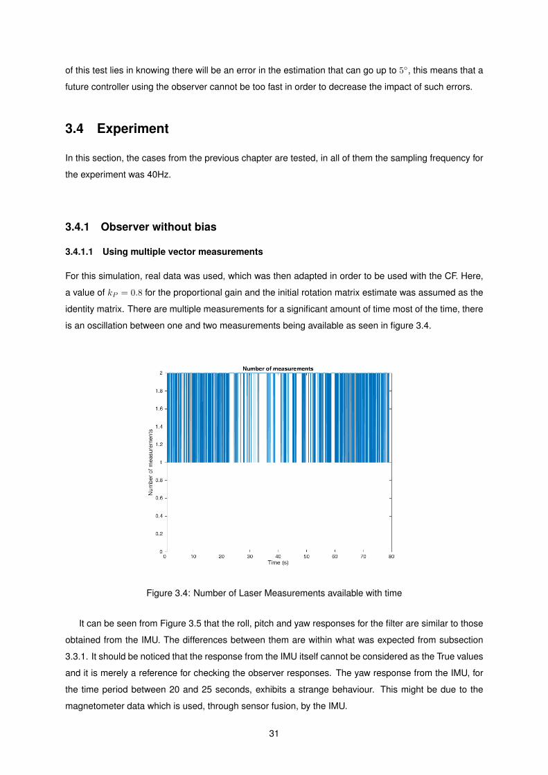
3.4.1.1 Using multiple vector measurements
For this simulation, real data was used, which was then adapted in order to be used with the CF. Here,
a value of kP = 0.8 for the proportional gain and the initial rotation matrix estimate was assumed as the
identity matrix. There are multiple measurements for a significant amount of time most of the time, there
is an oscillation between one and two measurements being available as seen in figure 3.4.
Figure 3.4: Number of Laser Measurements available with time
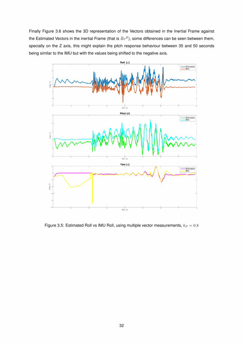
It can be seen from Figure 3.5 that the roll, pitch and yaw responses for the filter are similar to those
obtained from the IMU. The differences between them are within what was expected from subsection
3.3.1. It should be noticed that the response from the IMU itself cannot be considered as the True values
and it is merely a reference for checking the observer responses. The yaw response from the IMU, for
the time period between 20 and 25 seconds, exhibits a strange behaviour. This might be due to the
magnetometer data which is used, through sensor fusion, by the IMU.
31
Finally Figure 3.6 shows the 3D representation of the Vectors obtained in the Inertial Frame against
the Estimated Vectors in the inertial Frame (that is RvB), some differences can be seen between them,
specially on the Z axis, this might explain the pitch response behaviour between 35 and 50 seconds
being similar to the IMU but with the values being shifted to the negative axis.
Figure 3.5: Estimated Roll vs IMU Roll, using multiple vector measurements, kP = 0.8
32
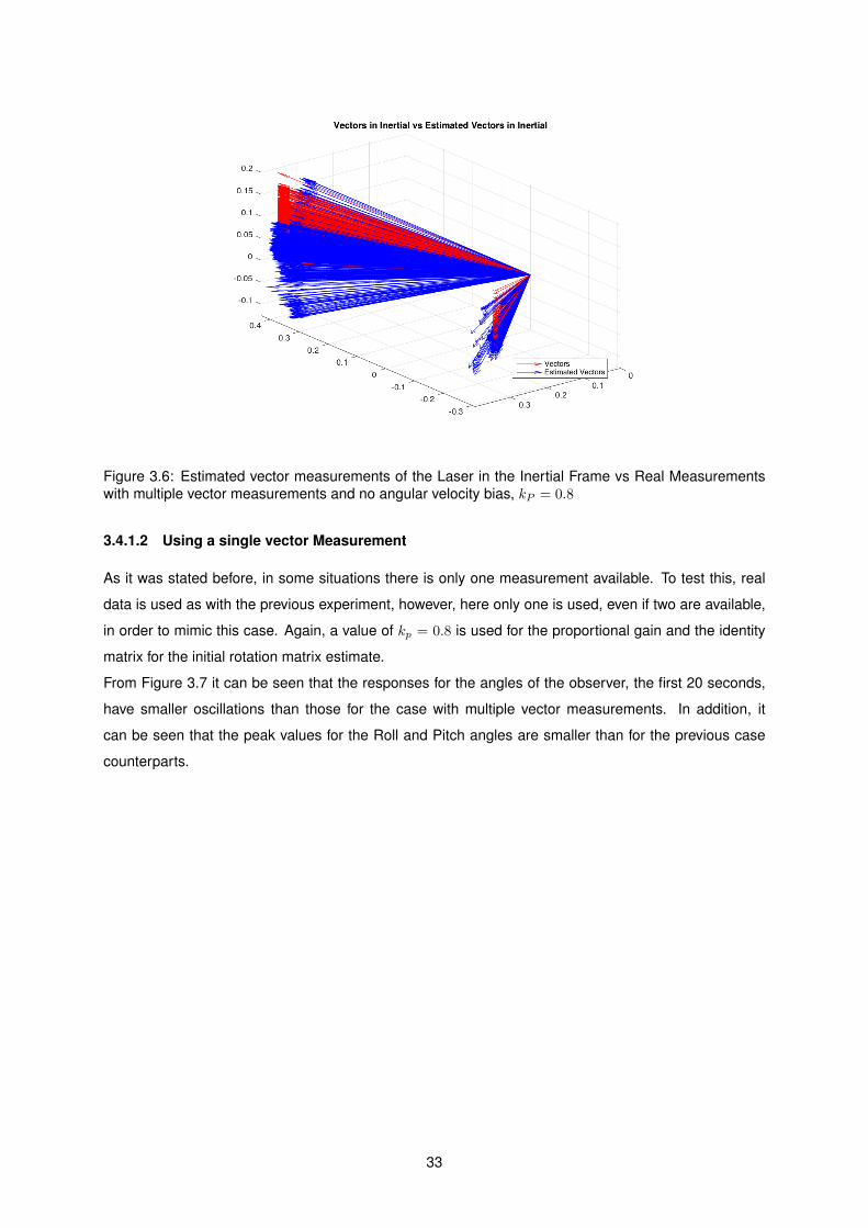
Figure 3.6: Estimated vector measurements of the Laser in the Inertial Frame vs Real Measurementswith multiple vector measurements and no angular velocity bias, kP = 0.8
3.4.1.2 Using a single vector Measurement
As it was stated before, in some situations there is only one measurement available. To test this, real
data is used as with the previous experiment, however, here only one is used, even if two are available,
in order to mimic this case. Again, a value of kp = 0.8 is used for the proportional gain and the identity
matrix for the initial rotation matrix estimate.
From Figure 3.7 it can be seen that the responses for the angles of the observer, the first 20 seconds,
have smaller oscillations than those for the case with multiple vector measurements. In addition, it
can be seen that the peak values for the Roll and Pitch angles are smaller than for the previous case
counterparts.
33
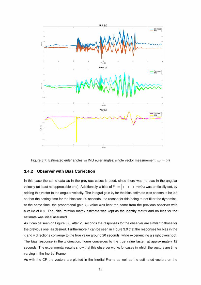
Figure 3.7: Estimated euler angles vs IMU euler angles, single vector measurement, kP = 0.8
3.4.2 Observer with Bias Correction
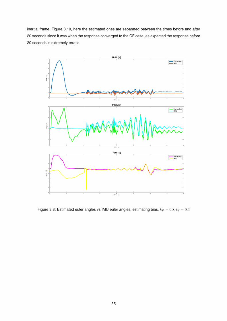
In this case the same data as in the previous cases is used, since there was no bias in the angular
velocity (at least no appreciable one). Additionally, a bias of bT =[1 1 1
]rad/s was artificially set, by
adding this vector to the angular velocity. The integral gain kI for the bias estimate was chosen to be 0.3
so that the setting time for the bias was 20 seconds, the reason for this being to not filter the dynamics,
at the same time, the proportional gain kP value was kept the same from the previous observer with
a value of 0.8. The initial rotation matrix estimate was kept as the identity matrix and no bias for the
estimate was initial assumed.
As it can be seen on Figure 3.8, after 20 seconds the responses for the observer are similar to those for
the previous one, as desired. Furthermore it can be seen in Figure 3.9 that the responses for bias in the
x and y directions converge to the true value around 20 seconds, while experiencing a slight overshoot.
The bias response in the z direction, figure converges to the true value faster, at approximately 12
seconds. The experimental results show that this observer works for cases in which the vectors are time
varying in the Inertial Frame.
As with the CF, the vectors are plotted in the Inertial Frame as well as the estimated vectors on the
34
inertial frame, Figure 3.10, here the estimated ones are separated between the times before and after
20 seconds since it was when the response converged to the CF case, as expected the response before
20 seconds is extremely erratic.
Figure 3.8: Estimated euler angles vs IMU euler angles, estimating bias, kP = 0.8, kI = 0.3
35
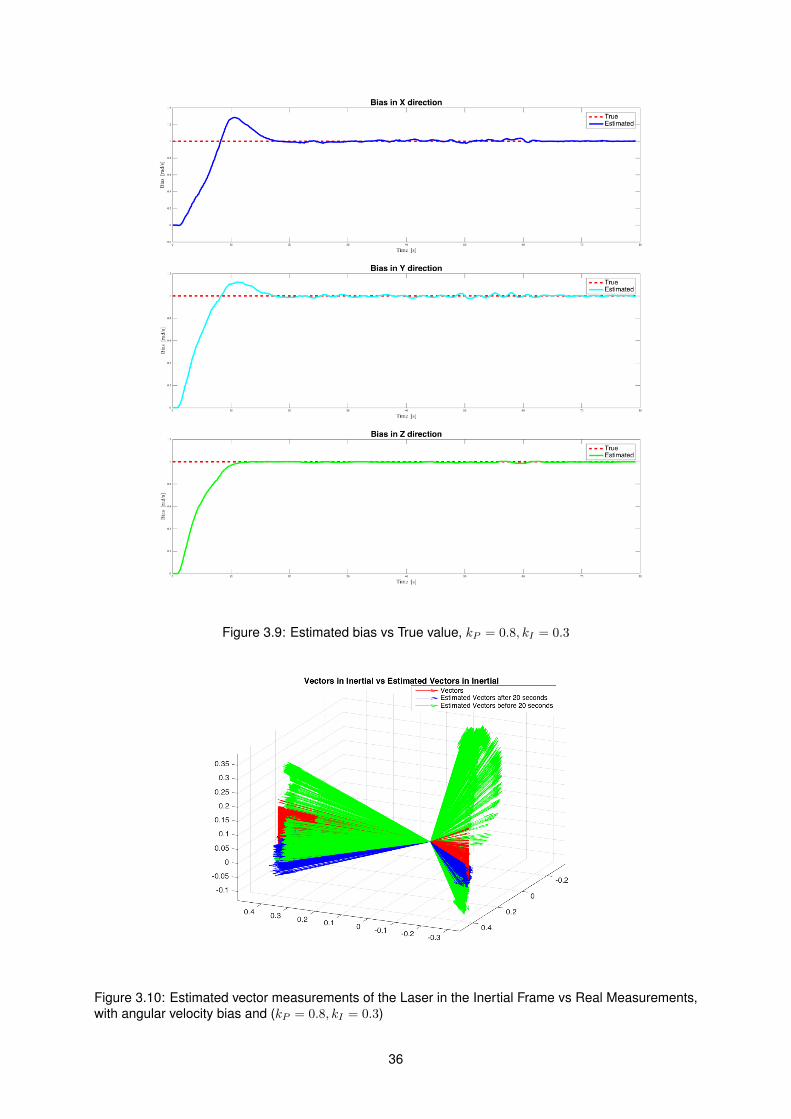
Figure 3.9: Estimated bias vs True value, kP = 0.8, kI = 0.3
Figure 3.10: Estimated vector measurements of the Laser in the Inertial Frame vs Real Measurements,with angular velocity bias and (kP = 0.8, kI = 0.3)
36
Chapter 4
Position and Attitude Control
When one wants to follow a desired trajectory, position control is also necessary. Building on the work in
[23], the developed controller belongs to the class of Hierarchical Controllers, where the Attitude Control
loop (Inner Loop) is faster then the Position Control Loop (Outer Loop). It is important to notice, that
this analysis does not consider the fact the attitude fed to the controller is estimated, as stated in the
following assumption.
Assumption 1.
The dynamics between the angular velocity error are negligible, as one assumes the angular velocity is
driven to the desired one instantaneously.
4.1 Outer Loop - Position Control
The system dynamics of a quadcopter are considered to be given by the system of equations
x = v
v = ge3 − Tmr3
(4.1)
where T is the scalar thrust applied to the vehicle and r3 as the third column vector of the rotation matrix
from {B} to {I}, g is the acceleration due to gravity, and e3 is third versor that defines the coordinate
system. The error dynamics of the system to be controlled are then given by
˙x = v
˙v = ge3 − Tmr3 − vd
. (4.2)
The error in the angular velocity is not needed, as the system is going to be actuated in thrust and angular
velocity. The errors for position and velocity are defined as x = x − xd and v = v − vd, respectively, in
37
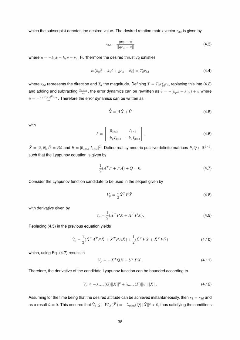
which the subscript d denotes the desired value. The desired rotation matrix vector r3d is given by
r3d =ge3 − u||ge3 − u||
(4.3)
where u = −kpx− kv v + vd. Furthermore the desired thrust Td satisfies
m(kpx+ kv v + ge3 − vd) = Tdr3d (4.4)
where r3d represents the direction and Td the magnitude. Defining T = TdrT3dr3, replacing this into (4.2)
and adding and subtracting Tdr3dm , the error dynamics can be rewritten as ˙v = −(kpx + kv v) + u where
u = −TdS(r3)2r3d
m . Therefore the error dynamics can be written as
˙X = AX + U (4.5)
with
A =
03×3 I3×3
−kpI3×3 −kvI3×3
, (4.6)
X = [x, v], U = Bu and B = [03×3 I3×3]T . Define real symmetric positive definite matrices P,Q ∈ R6×6,
such that the Lyapunov equation is given by
1
2(ATP + PA) +Q = 0. (4.7)
Consider the Lyapunov function candidate to be used in the sequel given by
Vp =1
2XTPX. (4.8)
with derivative given by
Vp =1
2( ˙XTPX + XTP˙X). (4.9)
Replacing (4.5) in the previous equation yields
Vp =1
2(XTATPX + XTPAX) +
1
2(UTPX + XTPU) (4.10)
which, using Eq. (4.7) results in
Vp = −XTQX + UTPX. (4.11)
Therefore, the derivative of the candidate Lyapunov function can be bounded according to
Vp ≤ −λmin(Q)||X||2 + λmax(P )||u||||X||. (4.12)
Assuming for the time being that the desired attitude can be achieved instantaneously, then r3 = r3d and
as a result u = 0. This ensures that Vp ≤ −WQ(X) = −λmin(Q)‖X‖2 < 0, thus satisfying the conditions
38
of Theorem 2, yielding asymptotic stability of the origin X = 0. Further on, the constants will be defined
in order to achieve the stability of the complete system even without considering this simplification. The
norm of u can be written as ||u|| = Td
m ||S(r3)r3d||, where the fact of ||S(r3)2r3d|| = ||S(r3)r3d|| was used.
Substituting this result plus using the triangular inequality, equation (4.12) can be rewritten as
Vp ≤ −λmin(Q)(||x||2 + ||v||2) + λmax(P )Tdm||S(r3)r3d||(||x||+ ||v||). (4.13)
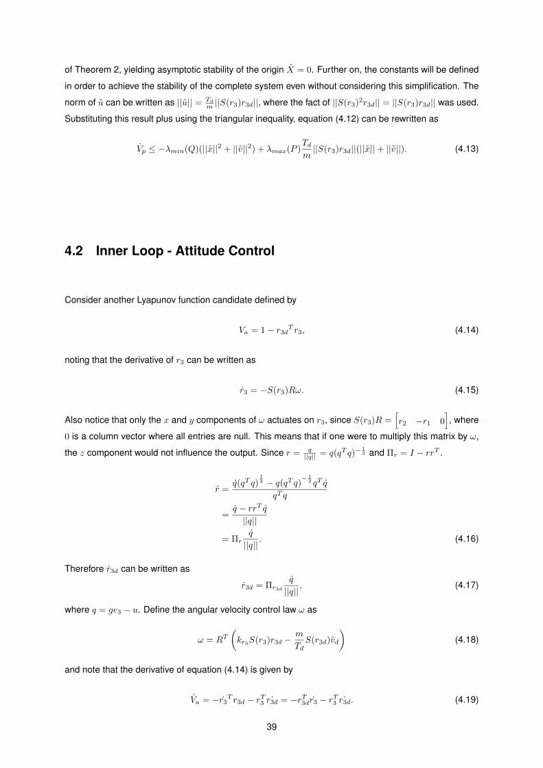
4.2 Inner Loop - Attitude Control
Consider another Lyapunov function candidate defined by
Va = 1− r3dT r3, (4.14)
noting that the derivative of r3 can be written as
r3 = −S(r3)Rω. (4.15)
Also notice that only the x and y components of ω actuates on r3, since S(r3)R =[r2 −r1 0
], where
0 is a column vector where all entries are null. This means that if one were to multiply this matrix by ω,
the z component would not influence the output. Since r = q||q|| = q(qT q)−
12 and Πr = I − rrT .
r =q(qT q)
12 − q(qT q)−
12 qT q
qT q
=q − rrT q||q||
= Πrq
||q||. (4.16)
Therefore r3d can be written as
r3d = Πr3d
q
||q||, (4.17)
where q = ge3 − u. Define the angular velocity control law ω as
ω = RT(kr3S(r3)r3d −
m
TdS(r3d)vd
)(4.18)
and note that the derivative of equation (4.14) is given by
Va = −r3T r3d − rT3 ˙r3d = −rT3dr3 − rT3 ˙r3d. (4.19)
39
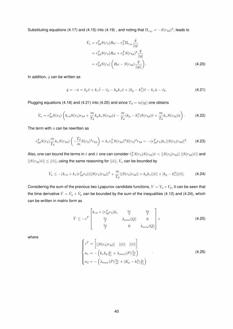
Substituting equations (4.17) and (4.15) into (4.19) , and noting that Πr3d = −S(r3d)2, leads to
Va = rT3dS(r3)Rω − rT3 Πr3d
q
||q|
= rT3dS(r3)Rω + rT3 S(r3d)2 q
||q|
= rT3dS(r3)
(Rω − S(r3d)
q
||q||
). (4.20)
In addition, q can be written as
q = −u = kpv + kv ˙v − vd − kpkvx+ (kp − k2v)v − kvu− vd. (4.21)
Plugging equations (4.18) and (4.21) into (4.20) and since Td = m||q|| one obtains
Va = rT3dS(r3)
(kr3S(r3)r3d +
m
TdkpkvS(r3d)x−
m
Td(kp − k2v)S(r3d)v +
m
TdkvS(r3d)u
). (4.22)
The term with u can be rewritten as
rT3dS(r3)m
TdkvS(r3d)
(−TdmS(r3)2r3d
)= kvr
T3 S(r3d)
2S(r3)2r3d = −(rT3dr3)kv||S(r3)r3d||2. (4.23)
Also, one can bound the terms in v and x one can consider rT3 S(r3)S(r3d)v < ||S(r3)r3d|| ||S(r3d)v|| and
||S(r3d)v|| ≤ ||v||, using the same reasoning for ||x||, Va can be bounded by
Va ≤ −(kr3 + kv(rT3dr3))||S(r3)r3d||2 +
m
Td||S(r3)r3d||+ kpkv||x||+ |kp − k2v|||v||. (4.24)
Considering the sum of the previous two Lyapunov candidate functions, V = Va+Vp, it can be seen that
the time derivative V = Va + Vp can be bounded by the sum of the inequalities (4.12) and (4.24), which
can be written in matrix form as
V ≤ −zT
kr3 + (rT3dr3)kv
n1
2n2
2
n1
2 λmin(Q) 0
n2
2 0 λmin(Q)
z (4.25)
where zT =
[||S(r3)r3d|| ||x|| ||v||
]n1 = −
(kvkp
mTd
+ λmax(P )Td
m
)n2 = −
(λmax(P )Td
m + |Kp − k2v|mTd
) . (4.26)
40
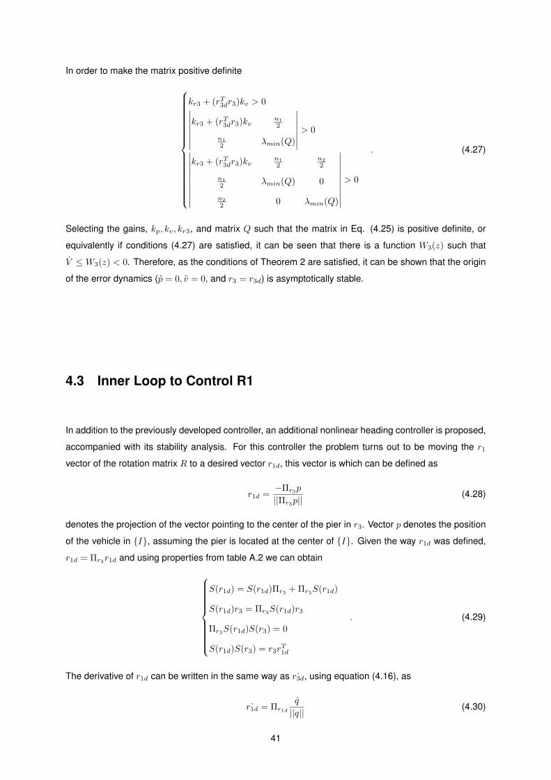
In order to make the matrix positive definite
kr3 + (rT3dr3)kv > 0∣∣∣∣∣∣∣kr3 + (rT3dr3)kv
n1
2
n1
2 λmin(Q)
∣∣∣∣∣∣∣ > 0
∣∣∣∣∣∣∣∣∣∣kr3 + (rT3dr3)kv
n1
2n2
2
n1
2 λmin(Q) 0
n2
2 0 λmin(Q)
∣∣∣∣∣∣∣∣∣∣> 0
. (4.27)
Selecting the gains, kp, kv, kr3, and matrix Q such that the matrix in Eq. (4.25) is positive definite, or
equivalently if conditions (4.27) are satisfied, it can be seen that there is a function W3(z) such that
V ≤ W3(z) < 0. Therefore, as the conditions of Theorem 2 are satisfied, it can be shown that the origin
of the error dynamics (p = 0, v = 0, and r3 = r3d) is asymptotically stable.
4.3 Inner Loop to Control R1
In addition to the previously developed controller, an additional nonlinear heading controller is proposed,
accompanied with its stability analysis. For this controller the problem turns out to be moving the r1
vector of the rotation matrix R to a desired vector r1d, this vector is which can be defined as
r1d =−Πr3p
||Πr3p||(4.28)
denotes the projection of the vector pointing to the center of the pier in r3. Vector p denotes the position
of the vehicle in {I}, assuming the pier is located at the center of {I}. Given the way r1d was defined,
r1d = Πr3r1d and using properties from table A.2 we can obtain
S(r1d) = S(r1d)Πr3 + Πr3S(r1d)
S(r1d)r3 = Πr3S(r1d)r3
Πr3S(r1d)S(r3) = 0
S(r1d)S(r3) = r3rT1d
. (4.29)
The derivative of r1d can be written in the same way as ˙r3d, using equation (4.16), as
˙r1d = Πr1d
q
||q||(4.30)
41
where in this case q = −Πr3p. It is helpful to rewrite r3 in a different way from (4.15) in order to have
terms in r1 and r3, this is done by considering ω = [ωx ωy ωz]T , and is given by
r3 = −S(r3)Rω
= −ωxS(r3)r1 + ωyr1. (4.31)
The term q can be written as
q = − ˙Πr3p−Πr3 p
= r3rT3 + r3r3
T −Πr3v
=(−ωxS(r3)r1r
T3 + ωyr1r
T3 + ωxr3r
T1 S(r3) + r3r
T1 ωy
)p−Πr3v
=(−ωxS(r3)r1r
T3 + ωyr1r
T3 + ωxS(r1)S(r3)S(r3) + ωyS(r1)S(r3)
)p−Πr3v
=(−ωxS(r3)r1r
T3 + ωyr1r
T3 − ωxS(r1)Πr3 + ωyS(r1)S(r3)Πr3
)p−Πr3v
=(−ωxS(r3)r1r
T3 + ωyr1r
T3
)p−Πr3v − (ωxS(r1)− ωyS(r1)S(r3)) Πr3p
=(−ωxS(r3)r1r
T3 + ωyr1r
T3
)p−Πr3v + (ωxS(r1)− ωyS(r1)S(r3)) r1d||q||. (4.32)
Using the result obtained from the transformation (4.32) one can rewrite ˙r1d as
˙r1d =Πr1d
||q||((−ωxS(r3)r1r
T3 + ωyr1r
T3
)p−Πr3v
)+ Πr1d (ωxS(r1)− ωyS(r1)S(r3)) r1d
=Πr1d
||q||((−ωxS(r3)r1r
T3 + ωyr1r
T3
)p−Πr3v
)+ (ωxS(r1)− ωyS(r1)S(r3)) r1d (4.33)
where the second step uses the fact rT1dS(r1)S(r3) = rT1dr3rT1 = 0, and it is important to notice that if
one does the inner product between r1 and ˙r1d, the second term dependent on r1d disappears. The
derivative of r1, considering ωT =[ωx ωy ωz
], can be written in a similar way to that of r3 as
r1 = −S(r1)Rω. (4.34)
To prove the stability of the control input chosen, the Lyapunov function candidate is chosen as
Vr1 = 1− rT1 r1d. (4.35)
Differentiating equation (4.35), one obtains
Vr1 = −r1T r1d − rT1 ˙r1d = −r1dT r1 − rT1 ˙r1d. (4.36)
42
Plugging equations (4.34) and (4.33) into (4.36), results in
Vr1 = rT1dS(r1)Rω − rT1 ˙r1d
= rT1d
[0 r3 −r2
]ω − rT1
Πr1d
||q||((−ωxS(r3)r1r
T3 + ωyr1r
T3
)p−Πr3v
)= −rT1dS(r3)2
[0 r3 −r2
]ω + rT1
S(r1d)2
||q||((−ωxS(r3) + ωy) r1r
T3 p−Πr3v
)= −rT1dS(r3)
[0 0 r1
]ω − rT1d
S(r1)S(r1d)
||q||((−ωxS(r3) + ωy) r1r
T3 p−Πr3v
)= rT1dS(r1)
[0 0 r3
]ω − rT1d
S(r1)
||q||((−ωxS(r1d)S(r3) + ωyS(r1d)) r1r
T3 p+ S(r1d)S(r3)2v
)= rT1dS(r1)r3ωz − rT1d
S(r1)
||q||((−ωxS(r1d)S(r3)S(r3) + ωyS(r1d)S(r3))S(r1)p+ S(r1d)S(r3)2v
)= rT1dS(r1)r3ωz − rT1d
S(r1)
||q||(r3r
T1d (−ωxS(r3) + ωyI)S(r1)p+ r3r
T1dS(r3)v
)= rT1dS(r1)r3
(ωz −
1
||q||(rT1d (−ωxS(r3) + ωyI)S(r1)p+ rT1dS(r3)v
)). (4.37)
In order to have only one negative definite term, the control action is defined as
ωz =1
||q||(rT1d (−ωxS(r3) + ωyI)S(r1)p+ rT1dS(r3)v
)− kr1rT1dS(r1)r3, (4.38)
where kr1 ∈ R+0 . Plugging the previously derived parts into (4.37), results in equation
Vr1 = −kr1(rT1dS(r3)r1)2 < 0. (4.39)
Selecting a positive gain kr1 , it can be seen that the lyapunov function derivative satisfies Vr1 ≤ −Wr1(z) =
−kr1(rT1dS(r3)r1)2 < 0. Therefore, as the conditions of Theorem 2 are satisfied, it can be shown that the
origin of the error dynamics (r1 = r1d) is asymptotically stable.
43
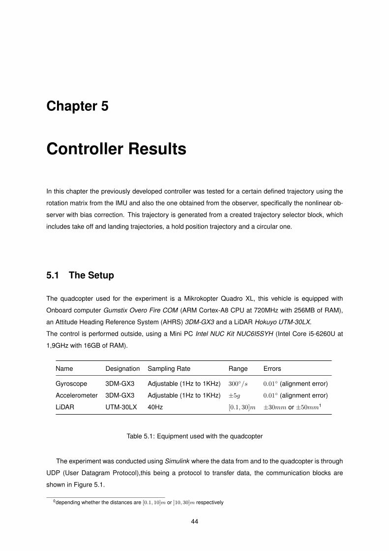
Chapter 5
Controller Results
In this chapter the previously developed controller was tested for a certain defined trajectory using the
rotation matrix from the IMU and also the one obtained from the observer, specifically the nonlinear ob-
server with bias correction. This trajectory is generated from a created trajectory selector block, which
includes take off and landing trajectories, a hold position trajectory and a circular one.
5.1 The Setup
The quadcopter used for the experiment is a Mikrokopter Quadro XL, this vehicle is equipped with
Onboard computer Gumstix Overo Fire COM (ARM Cortex-A8 CPU at 720MHz with 256MB of RAM),
an Attitude Heading Reference System (AHRS) 3DM-GX3 and a LiDAR Hokuyo UTM-30LX.
The control is performed outside, using a Mini PC Intel NUC Kit NUC6I5SYH (Intel Core i5-6260U at
1,9GHz with 16GB of RAM).
Name Designation Sampling Rate Range Errors
Gyroscope 3DM-GX3 Adjustable (1Hz to 1KHz) 300◦/s 0.01◦ (alignment error)
Accelerometer 3DM-GX3 Adjustable (1Hz to 1KHz) ±5g 0.01◦ (alignment error)
LiDAR UTM-30LX 40Hz [0.1, 30]m ±30mm or ±50mm1
Table 5.1: Equipment used with the quadcopter
The experiment was conducted using Simulink where the data from and to the quadcopter is through
UDP (User Datagram Protocol),this being a protocol to transfer data, the communication blocks are
shown in Figure 5.1.
0depending whether the distances are [0.1, 10]m or ]10, 30]m respectively
44
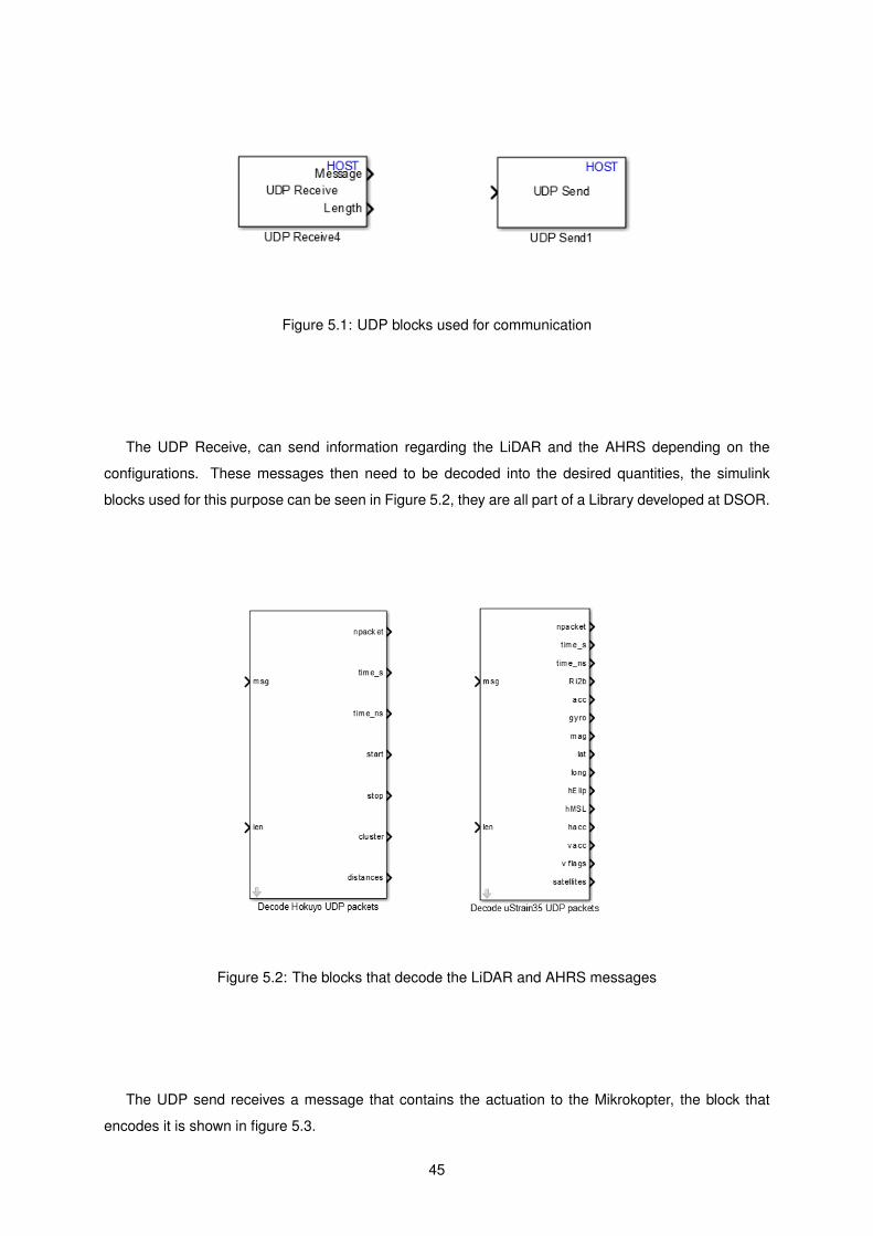
Figure 5.1: UDP blocks used for communication
The UDP Receive, can send information regarding the LiDAR and the AHRS depending on the
configurations. These messages then need to be decoded into the desired quantities, the simulink
blocks used for this purpose can be seen in Figure 5.2, they are all part of a Library developed at DSOR.
Figure 5.2: The blocks that decode the LiDAR and AHRS messages
The UDP send receives a message that contains the actuation to the Mikrokopter, the block that
encodes it is shown in figure 5.3.
45
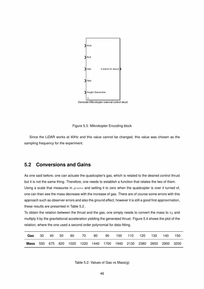
Figure 5.3: Mikrokopter Encoding block
Since the LiDAR works at 40Hz and this value cannot be changed, this value was chosen as the
sampling frequency for the experiment.
5.2 Conversions and Gains
As one said before, one can actuate the quadcopter’s gas, which is related to the desired control thrust
but it is not the same thing. Therefore, one needs to establish a function that relates the two of them.
Using a scale that measures in grams and setting it to zero when the quadcopter is over it turned of,
one can then see the mass decrease with the increase of gas. There are of course some errors with this
approach such as observer errors and also the ground effect, however it is still a good first approximation,
these results are presented in Table 5.2 .
To obtain the relation between the thrust and the gas, one simply needs to convert the mass to kg and
multiply it by the gravitational acceleration yielding the generated thrust. Figure 5.4 shows the plot of the
relation, where the one used a second order polynomial for data fitting.
Gas 30 40 50 60 70 80 90 100 110 120 130 140 150
Mass 550 675 820 1020 1220 1440 1700 1940 2130 2380 2650 2900 3200
Table 5.2: Values of Gas vs Mass(g)
46
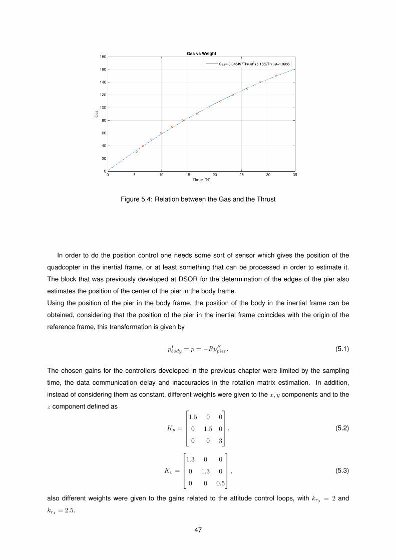
Figure 5.4: Relation between the Gas and the Thrust
In order to do the position control one needs some sort of sensor which gives the position of the
quadcopter in the inertial frame, or at least something that can be processed in order to estimate it.
The block that was previously developed at DSOR for the determination of the edges of the pier also
estimates the position of the center of the pier in the body frame.
Using the position of the pier in the body frame, the position of the body in the inertial frame can be
obtained, considering that the position of the pier in the inertial frame coincides with the origin of the
reference frame, this transformation is given by
pIbody = p = −RpBpier. (5.1)
The chosen gains for the controllers developed in the previous chapter were limited by the sampling
time, the data communication delay and inaccuracies in the rotation matrix estimation. In addition,
instead of considering them as constant, different weights were given to the x, y components and to the
z component defined as
Kp =
1.5 0 0
0 1.5 0
0 0 3
, (5.2)
Kv =
1.3 0 0
0 1.3 0
0 0 0.5
, (5.3)
also different weights were given to the gains related to the attitude control loops, with kr3 = 2 and
kr1 = 2.5.
47
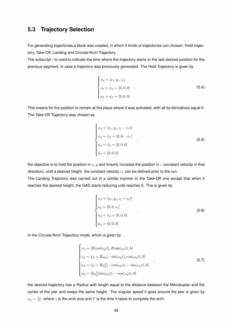
5.3 Trajectory Selection
For generating trajectories,a block was created, in which 4 kinds of trajectories can chosen: Hold trajec-
tory, Take-Off, Landing and Circular/Arch Trajectory.
The subscript i is used to indicate the time where the trajectory starts or the last desired position for the
previous segment, in case a trajectory was previously generated. The Hold Trajectory is given by
xd = [xi, yi, zi]
vd = xd = [0, 0, 0]
ad = ad = [0, 0, 0]
. (5.4)
This means for the position to remain at the place where it was activated, with all its derivatives equal 0.
The Take-Off Trajectory was chosen as
xd = [xi, yi, zi − vct]
vd = xd = [0, 0,−vc]
ad = vd = [0, 0, 0]
ad = [0, 0, 0]
, (5.5)
the objective is to hold the position in x, y and linearly increase the position in z (constant velocity in that
direction), until a desired height. the constant velocity vc can be defined prior to the run.
The Landing Trajectory was carried out in a similar manner to the Take-Off one except that when it
reaches the desired height, the GAS starts reducing until reaches 0. This is given by
xd = [xi, yi, zi + vct]
vd = [0, 0, vc]
ad = vd = [0, 0, 0]
ad = [0, 0, 0]
. (5.6)
In the Circular/Arch Trajectory mode, which is given by
xd = [R cos(ωpt), R sin(ωpt), h]
vd = xd = Rωp[− sin(ωpt), cos(ωpt), 0]
ad = vd = Rω2p[− cos(ωpt),− sin(ωpt), 0]
ad = Rω3p[sin(ωpt),− cos(ωpt), 0]
, (5.7)
the desired trajectory has a Radius with length equal to the distance between the Mikrokopter and the
center of the pier and keeps the same height. The angular speed it goes around the pier is given by
ωp = πsT , where s is the arch size and T is the time it takes to complete the arch.
48
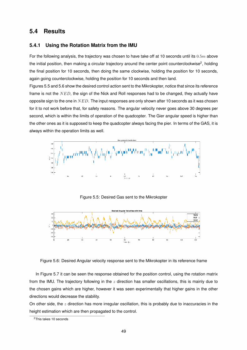
5.4 Results
5.4.1 Using the Rotation Matrix from the IMU
For the following analysis, the trajectory was chosen to have take off at 10 seconds until its 0.5m above
the initial position, then making a circular trajectory around the center point counterclockwise2, holding
the final position for 10 seconds, then doing the same clockwise, holding the position for 10 seconds,
again going counterclockwise, holding the position for 10 seconds and then land.
Figures 5.5 and 5.6 show the desired control action sent to the Mikrokopter, notice that since its reference
frame is not the NED, the sign of the Nick and Roll responses had to be changed, they actually have
opposite sign to the one inNED. The input responses are only shown after 10 seconds as it was chosen
for it to not work before that, for safety reasons. The angular velocity never goes above 30 degrees per
second, which is within the limits of operation of the quadcopter. The Gier angular speed is higher than
the other ones as it is supposed to keep the quadcopter always facing the pier. In terms of the GAS, it is
always within the operation limits as well.
Figure 5.5: Desired Gas sent to the Mikrokopter
Figure 5.6: Desired Angular velocity response sent to the Mikrokopter in its reference frame
In Figure 5.7 it can be seen the response obtained for the position control, using the rotation matrix
from the IMU. The trajectory following in the z direction has smaller oscillations, this is mainly due to
the chosen gains which are higher, however it was seen experimentally that higher gains in the other
directions would decrease the stability.
On other side, the z direction has more irregular oscillation, this is probably due to inaccuracies in the
height estimation which are then propagated to the control.2This takes 10 seconds
49
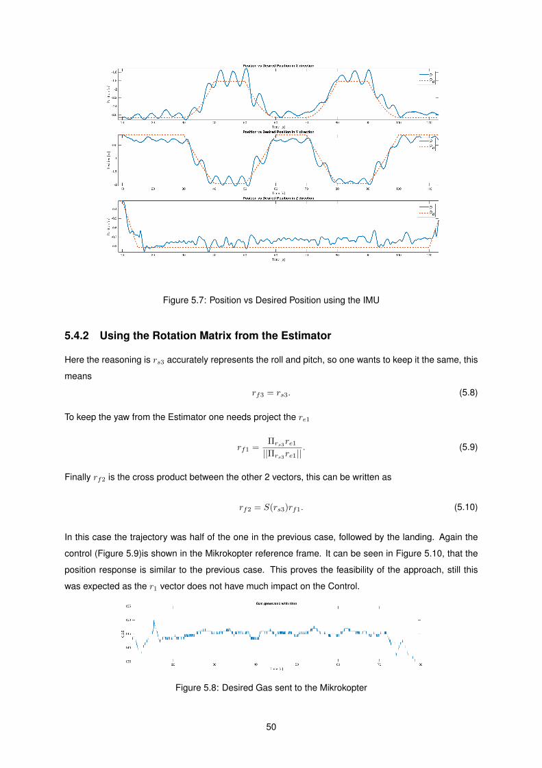
Figure 5.7: Position vs Desired Position using the IMU
5.4.2 Using the Rotation Matrix from the Estimator
Here the reasoning is rs3 accurately represents the roll and pitch, so one wants to keep it the same, this
means
rf3 = rs3. (5.8)
To keep the yaw from the Estimator one needs project the re1
rf1 =Πrs3re1||Πrs3re1||
. (5.9)
Finally rf2 is the cross product between the other 2 vectors, this can be written as
rf2 = S(rs3)rf1. (5.10)
In this case the trajectory was half of the one in the previous case, followed by the landing. Again the
control (Figure 5.9)is shown in the Mikrokopter reference frame. It can be seen in Figure 5.10, that the
position response is similar to the previous case. This proves the feasibility of the approach, still this
was expected as the r1 vector does not have much impact on the Control.
Figure 5.8: Desired Gas sent to the Mikrokopter
50
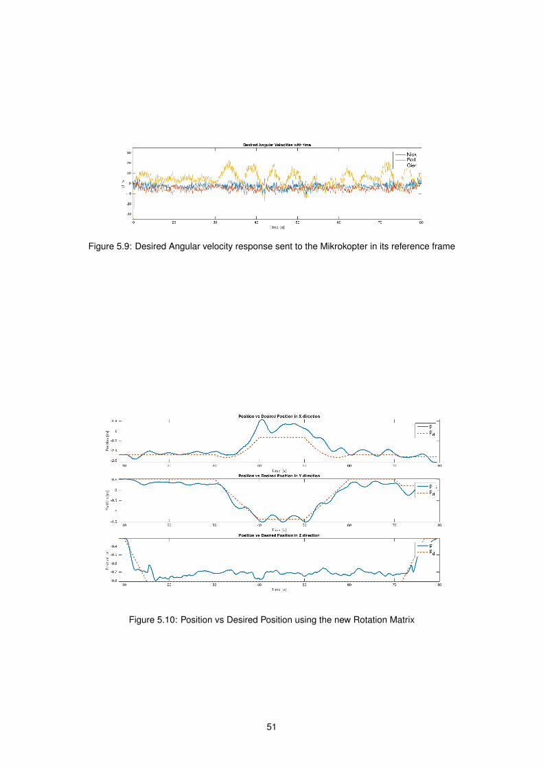
Figure 5.9: Desired Angular velocity response sent to the Mikrokopter in its reference frame
Figure 5.10: Position vs Desired Position using the new Rotation Matrix
51
Chapter 6
Conclusions
The main conclusion with this work is that it is possible to control the attitude and position of a quad-
copter in a GPS denied environment using LiDAR for the position and attitude estimation.
It was theoretically proven that the observer works for with multiple vector measurements as well as
when there is only a time varying vector measurement. In addition it was also proven that the observer
with Bias Correction, can indeed estimate attitude correctly.
Experimentally, using a quadcopter equipped with LiDAR it was seen that using only one vector mea-
surement presents a larger error. This might be due to the theory not having into consideration the
existence of noise in the vector measurement or needing more time for convergence.
The complete developed controller, which includes a nonlinear hierarchical controller for position and
attitude and the nonlinear heading controller, is stable and can be used with LiDAR data for position
control relative to a pier.
The controllers were successfully implemented in a Mikrokopter Quadro XL, using the rotation matrix
given by the IMU and yielded a good trajectory following considering the limitations. Using the observer
for the control, it was not possible to achieve satisfying results since the errors in the estimation for the
pitch and roll were to high. It is possible however to still use just the yaw estimation part of the observer
for the control with some mathematical manipulation.
6.1 Future Work
As future work the Quadcopter should be redesigned in order to have the NUC inside it, this would then
remove the communication delays. Still regarding the redesign, the arms should be bigger in order for
the rays used for the altitude determination to not be reflected on the quadcopter’s body.
Another possible development would be to test the performance with other LiDAR lasers, preferably
ones where the sampling rate could be changed.
52
Bibliography
[1] S. Waharte and N. Trigoni. Supporting search and rescue operations with uavs. In Emerging
Security Technologies (EST), 2010 International Conference on, pages 142–147. IEEE, 2010.
[2] S. Rathinam, P. Almeida, Z. Kim, S. Jackson, A. Tinka, W. Grossman, and R. Sengupta. Au-
tonomous searching and tracking of a river using an uav. In American Control Conference, 2007.
ACC’07, pages 359–364. IEEE, 2007.
[3] Amazon.com. Amazon prime air, 2016. URL http://www.amazon.com/b?node=8037720011.
[4] H. D. Black. A passive system for determining the attitude of a satellite. AIAA Journal, 2(7):1350–
1351, 1964.
[5] G. Wahba. A least squares estimate of satellite attitude. SIAM review, 7(3):409–409, 1965.
[6] M.-D. Hua, G. Ducard, T. Hamel, and R. Mahony. Introduction to nonlinear attitude estimation for
aerial robotic systems. Aerospace Lab, pages AL08–04, 2014.
[7] J. L. Crassidis, F. L. Markley, and Y. Cheng. Survey of nonlinear attitude estimation methods.
Journal of Guidance, Control, and Dynamics, 30(1):12–28, 2007.
[8] J. K. Thienel. Nonlinear observer/controller designs for spacecraft attitude control systems with
uncalibrated gyros. 2004.
[9] G. Troni and L. L. Whitcomb. Adaptive estimation of measurement bias in three-dimensional field
sensors with angular rate sensors: Theory and comparative experimental evaluation. In Robotics:
Science and Systems, 2013.
[10] H. F. Grip, T. I. Fossen, T. A. Johansen, and A. Saberi. Attitude estimation based on time-varying
reference vectors with biased gyro and vector measurements. Proc. IFAC World Congr., Milan,
Italy, pages 8497–8502, 2011.
[11] R. Mahony, T. Hamel, and J.-M. Pflimlin. Nonlinear complementary filters on the special orthogonal
group. Automatic Control, IEEE Transactions on, 53(5):1203–1218, 2008.
[12] K. J. Jensen. Generalized nonlinear complementary attitude filter. Journal of Guidance, Control,
and Dynamics, 34(5):1588–1593, 2011.
53
[13] R. Mahony, T. Hamel, J. Trumpf, and C. Lageman. Nonlinear attitude observers on so (3) for
complementary and compatible measurements: A theoretical study. In Decision and Control, 2009
held jointly with the 2009 28th Chinese Control Conference. CDC/CCC 2009. Proceedings of the
48th IEEE Conference on, pages 6407–6412. IEEE, 2009.
[14] A. Khosravian and M. Namvar. Globally exponential estimation of satellite attitude using a single
vector measurement and gyro. In Decision and Control (CDC), 2010 49th IEEE Conference on,
pages 364–369. IEEE, 2010.
[15] H. F. Grip, T. Fossen, T. A. Johansen, A. Saberi, et al. Attitude estimation using biased gyro and
vector measurements with time-varying reference vectors. Automatic Control, IEEE Transactions
on, 57(5):1332–1338, 2012.
[16] S. Bras, R. Cunha, J. F. Vasconcelos, C. Silvestre, and P. Oliveira. A nonlinear attitude observer
based on active vision and inertial measurements. Robotics, IEEE Transactions on, 27(4):664–677,
2011.
[17] M.-D. Hua, G. Ducard, T. Hamel, R. Mahony, and K. Rudin. Implementation of a nonlinear attitude
estimator for aerial robotic vehicles. Control Systems Technology, IEEE Transactions on, 22(1):
201–213, 2014.
[18] A. Khosravian, J. Trumpf, R. Mahony, and T. Hamel. Recursive attitude estimation in the presence
of multi-rate and multi-delay vector measurements,”. In American Control Conference, vol.-, 2015.
[19] M.-D. Hua, T. Hamel, P. Morin, and C. Samson. Introduction to feedback control of underactuated
vtolvehicles: A review of basic control design ideas and principles. IEEE Control Systems, 33(1):
61–75, 2013.
[20] A. Gomes. Laser-based control of rotary-wing uavs. Master’s thesis, Instituto Superior Tecnico,
2015.
[21] R. Mahony, T. Hamel, and J.-M. Pflimlin. Complementary filter design on the special orthogonal
group so (3). In Decision and Control, 2005 and 2005 European Control Conference. CDC-ECC’05.
44th IEEE Conference on, pages 1477–1484. IEEE, 2005.
[22] N. A. Chaturvedi, A. K. Sanyal, and N. H. McClamroch. Rigid-body attitude control. Control Sys-
tems, IEEE, 31(3):30–51, 2011.
[23] R. Santos. Load transportation using rotary-wing uavs. Master’s thesis, Instituto Superior Tecnico,
2015.
[24] J. Vasconcelos, R. Cunha, C. Silvestre, and P. Oliveira. Landmark based nonlinear observer for
rigid body attitude and position estimation. In Decision and Control, 2007 46th IEEE Conference
on, pages 1033–1038. IEEE, 2007.
[25] A. Khosravian, J. Trumpf, R. Mahony, and C. Lageman. Observers for invariant systems on lie
groups with biased input measurements and homogeneous outputs. Automatica, 55:19–26, 2015.
54
[26] J. Vasconcelos, R. Cunha, C. Silvestre, and P. Oliveira. Stability of a nonlinear attitude observer on
so (3) with nonideal angular velocity measurements. In Control Conference (ECC), 2009 European,
pages 2769–2774. IEEE, 2009.
[27] D. Choukroun. Novel methods for attitude determination using vector observations. PhD thesis,
Technion-Israel Institute of Technology, Faculty of Aerospace Engineering, 2003.
[28] M.-D. Hua, K. Rudin, G. Ducard, T. Hamel, and R. Mahony. Nonlinear attitude estimation with mea-
surement decoupling and anti-windup gyro-bias compensation. In IFAC World Congress, pages
2972–2978, 2011.
[29] A. Barrau and S. Bonnabel. Intrinsic filtering on lie groups with applications to attitude estimation.
Automatic Control, IEEE Transactions on, 60(2):436–449, 2015.
[30] H. K. Khalil and J. Grizzle. Nonlinear systems, volume 3. Prentice hall New Jersey, 1996.
[31] M. Brookes. The matrix reference manual, 2011. URL http://www.ee.imperial.ac.uk/hp/
staff/dmb/matrix/intro.html.
55

56
Appendix A
Mathematical Background
This chapter reviews several Mathematical concepts needed further on for mathematical proofs. Several
Algebraic properties are enumerated and a brief introduction to Non Linear System Theory is made.
A.1 Algebraic Properties
A square matrix can either be positive (semi-)definite, negative (semi-) definite or indefinite. A matrix N
is positive definite if xTNx > 0, positive semi-definite if xTNx ≥ 0, for any vector x different from zero,
noting that similar expressions for negative definite and negative semi-definite matrices can be defined,
but with opposite signs.
Every square matrix N can be written as a sum of symmetric and anti-symmetric (also called skew
symmetric) matrices (N = Ps(N) + Pa(N)). Ps(N) designates the symmetric part of the matrix N and
Pa(N) designates the anti symmetric part of the matrix. The properties in Table A.1 are always valid for
these kind of matrices.
Table A.1: List of properties valid for any square matrix, taken from [31]
Equation
Ps(N) = Ps(N)T
Pa(N) = −Pa(N)T
Ps(N) = N+NT
2
Pa(N) = N−NT
2
The angular velocity of rotation between two frames can be expressed as a skew-symmetric matrix
instead of a vector, also allowing to consider the cross-product of two vectors into a simpler case of
matrix multiplication. Throughout this thesis, the skew operator equation a × b = S(a)b, will be used
A.1
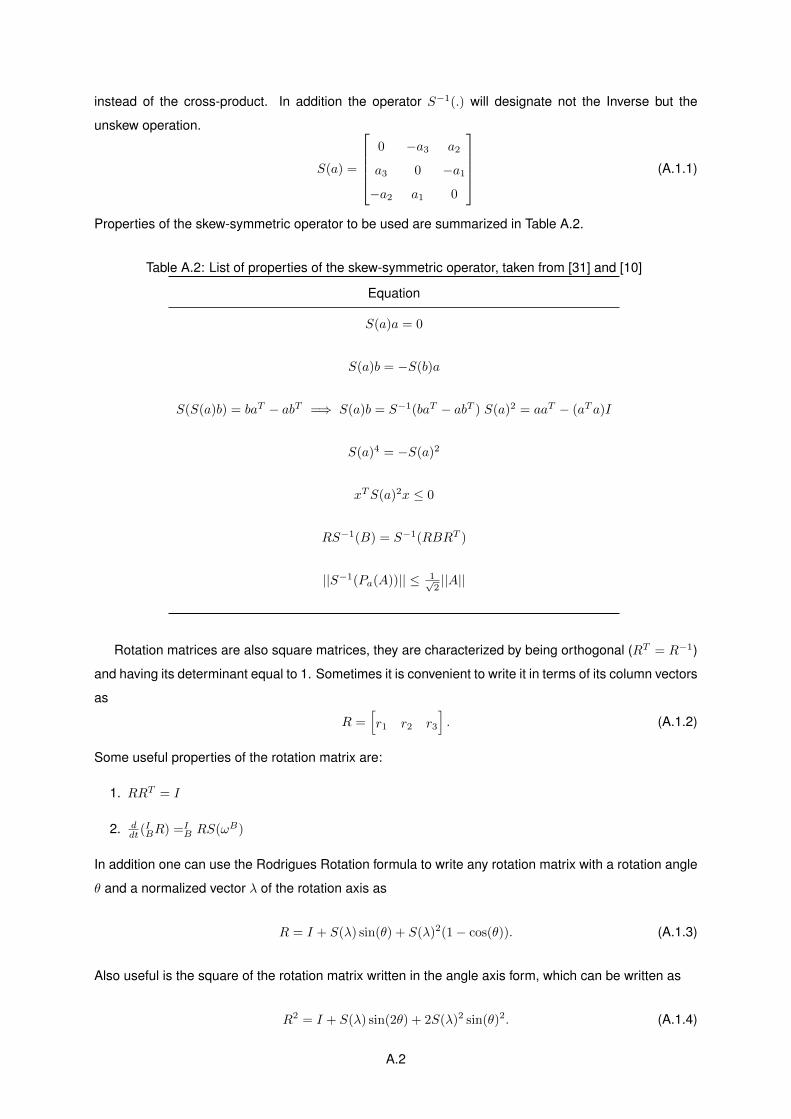
instead of the cross-product. In addition the operator S−1(.) will designate not the Inverse but the
unskew operation.
S(a) =
0 −a3 a2
a3 0 −a1−a2 a1 0
(A.1.1)
Properties of the skew-symmetric operator to be used are summarized in Table A.2.
Table A.2: List of properties of the skew-symmetric operator, taken from [31] and [10]
Equation
S(a)a = 0
S(a)b = −S(b)a
S(S(a)b) = baT − abT =⇒ S(a)b = S−1(baT − abT ) S(a)2 = aaT − (aTa)I
S(a)4 = −S(a)2
xTS(a)2x ≤ 0
RS−1(B) = S−1(RBRT )
||S−1(Pa(A))|| ≤ 1√2||A||
Rotation matrices are also square matrices, they are characterized by being orthogonal (RT = R−1)
and having its determinant equal to 1. Sometimes it is convenient to write it in terms of its column vectors
as
R =[r1 r2 r3
]. (A.1.2)
Some useful properties of the rotation matrix are:
1. RRT = I
2. ddt (
IBR) =I
B RS(ωB)
In addition one can use the Rodrigues Rotation formula to write any rotation matrix with a rotation angle
θ and a normalized vector λ of the rotation axis as
R = I + S(λ) sin(θ) + S(λ)2(1− cos(θ)). (A.1.3)
Also useful is the square of the rotation matrix written in the angle axis form, which can be written as
R2 = I + S(λ) sin(2θ) + 2S(λ)2 sin(θ)2. (A.1.4)
A.2
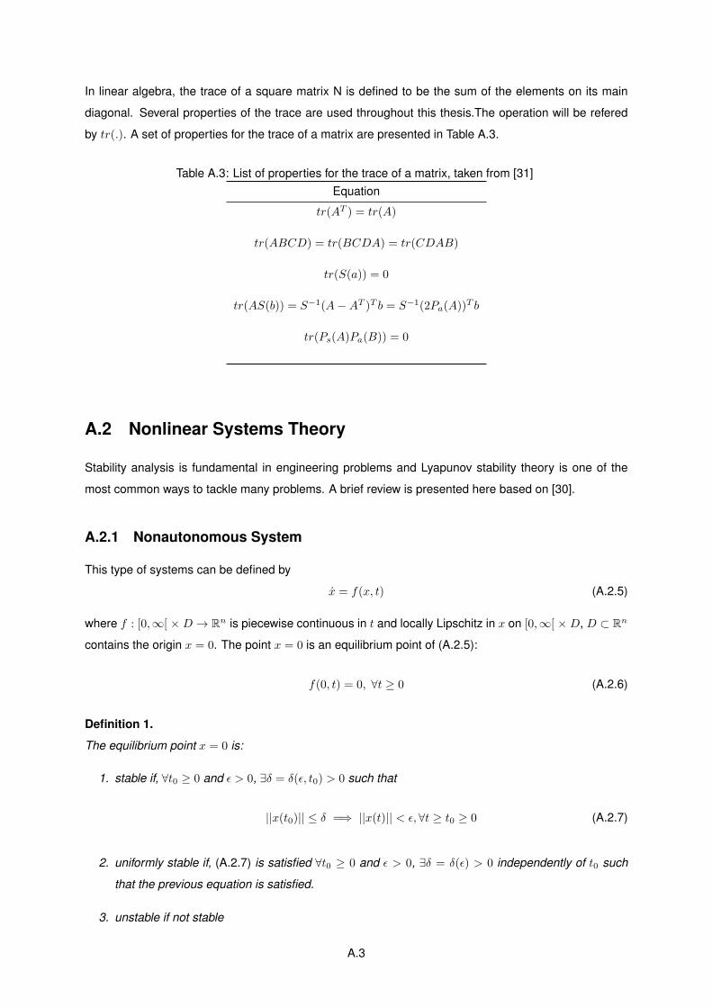
In linear algebra, the trace of a square matrix N is defined to be the sum of the elements on its main
diagonal. Several properties of the trace are used throughout this thesis.The operation will be refered
by tr(.). A set of properties for the trace of a matrix are presented in Table A.3.
Table A.3: List of properties for the trace of a matrix, taken from [31]Equation
tr(AT ) = tr(A)
tr(ABCD) = tr(BCDA) = tr(CDAB)
tr(S(a)) = 0
tr(AS(b)) = S−1(A−AT )T b = S−1(2Pa(A))T b
tr(Ps(A)Pa(B)) = 0
A.2 Nonlinear Systems Theory
Stability analysis is fundamental in engineering problems and Lyapunov stability theory is one of the
most common ways to tackle many problems. A brief review is presented here based on [30].
A.2.1 Nonautonomous System
This type of systems can be defined by
x = f(x, t) (A.2.5)
where f : [0,∞[ × D → Rn is piecewise continuous in t and locally Lipschitz in x on [0,∞[ × D, D ⊂ Rn
contains the origin x = 0. The point x = 0 is an equilibrium point of (A.2.5):
f(0, t) = 0, ∀t ≥ 0 (A.2.6)
Definition 1.
The equilibrium point x = 0 is:
1. stable if, ∀t0 ≥ 0 and ε > 0, ∃δ = δ(ε, t0) > 0 such that
||x(t0)|| ≤ δ =⇒ ||x(t)|| < ε,∀t ≥ t0 ≥ 0 (A.2.7)
2. uniformly stable if, (A.2.7) is satisfied ∀t0 ≥ 0 and ε > 0, ∃δ = δ(ε) > 0 independently of t0 such
that the previous equation is satisfied.
3. unstable if not stable
A.3
4. asymptotically stable if it is stable and there is a positive constant c = c(t0) such that x(t) → 0 as
t→∞ , ∀ ||x(t0)|| < c
5. uniformly asymptotically stable if it is uniformly stable and there is a positive constant c, indepen-
dent of t0 such that x(t)→ 0 as t→∞ uniformly in t0, ∀||x(t0)|| < c
6. globally uniformly asymptotically stable if uniformly stable, limε→∞ δ(ε) = ∞ and for each pair
a, c > 0,∃T (a, c) > 0 such that
||x(t)|| < a ∀t ≥ t0 + T (a, c), ||x(t0)|| < c (A.2.8)
Theorem 1.
Let x = 0 be an equilibrium point for (A.2.5) and D ∈ Rn be a domain containing that point. Let
V : [0,∞[×D → R be a continuously differentiable function such that:
W1(x) ≤ V (t, x) ≤W2(x) (A.2.9)
∂V
∂t+∂V
∂xf(t, x) ≤ 0 (A.2.10)
∀t ≥ 0 and ∀x ∈ D where W1 and W2 are continuous positive definite functions on D. Then x = 0 is
uniformly stable.
Theorem 2.
Suppose the assumptions from the previous theorem are satisfied with the inequality (A.2.10) strength-
ened to∂V
∂t+∂V
∂xf(t, x) ≤ −W3(x) (A.2.11)
∀t ≥ 0 and ∀x ∈ D where W3 is a continuous positive definite function on D. Then x = 0 is uniformly
asymptotically stable. Moreover, if r and c are chosen such that Br = {||x|| ≤ r} ⊂ D and c <
min||x||=rW1(x) then every trajectory starting in {x ∈ Br|W2(x) ≤ c} satisfies
||x(t)|| ≤ β(||x(t0)||, t− t0),∀t ≥ t0 ≥ 0. (A.2.12)
For some KL function β. Finally if D = Rn and W1(x) is radially unbounded, then x = 0 is globally
asymptotically stable.
The following Lemma is known as the Barbalat’s lemma, and is reproduced here as in [30].
Lemma 1.
Let φ : be a uniformly continuous function on [0,∞), suppose that limt→+∞∫ t0φ(τ)dτ exists and is finite.
Then,
φ(t)→ 0 as t→∞ (A.2.13)
A.4
Related Documents