Lewontin (1972) Rasmus Grønfeldt Winther 0000-0001-8976-3052 To appear in: Lorusso, L and Winther, R.G. 2022. Remapping Race in a Global Context. London: Routledge. **PENULTIMATE VERSION.** Abstract Richard C. Lewontin is arguably the most influential evolutionary biologist of the second half of the 20th century. In this chapter, I provide two windows on his influential 1972 article “The Apportionment of Human Diversity”: First, I show how the fourteen publications that he cites influenced him and framed his exploration; second, I present close readings of the five sections of the article: “Introduction,” “The Genes,” “The Samples,” “The Measure of Diversity,” and “The Results.” I hope to illuminate the article’s basic anatomy and argumentative arc, and why it became such a historically important document. In particular, I make explicit all of the mathematics (e.g., six Shannon information measures) and the general population genetic theory underlying this mathematics (e.g., the Wahlund effect). Lewontin did not make this explicit in his article. Furthermore, in redoing all of his calculations, I find that Lewontin made calculation errors (including rounding errors or omitting diversity component values) for all the genes he analyzed except one (P), and understated the among races diversity component, according to even just his own calculations. In reproducing the original computation, I find that the values of, respectively, within populations, among populations but within races, and among races diversity apportionments shift slightly (86%, 7%, 7%); here, in this “field guide” to Lewontin (1972), as well as in Winther (2022), I discuss this change in light of the values produced in subsequent replications of Lewontin’s calculation with other statistics and data sets.

Welcome message from author
This document is posted to help you gain knowledge. Please leave a comment to let me know what you think about it! Share it to your friends and learn new things together.
Transcript
Lewontin (1972)
Rasmus Grønfeldt Winther 0000-0001-8976-3052
To appear in:
Lorusso, L and Winther, R.G. 2022. Remapping Race in a Global
Context. London: Routledge.
**PENULTIMATE VERSION.**
Abstract
Richard C. Lewontin is arguably the most influential evolutionary biologist of the second half of
the 20th century. In this chapter, I provide two windows on his influential 1972 article “The
Apportionment of Human Diversity”: First, I show how the fourteen publications that he cites
influenced him and framed his exploration; second, I present close readings of the five sections of
the article: “Introduction,” “The Genes,” “The Samples,” “The Measure of Diversity,” and “The
Results.” I hope to illuminate the article’s basic anatomy and argumentative arc, and why it became
such a historically important document. In particular, I make explicit all of the mathematics (e.g.,
six Shannon information measures) and the general population genetic theory underlying this
mathematics (e.g., the Wahlund effect). Lewontin did not make this explicit in his article.
Furthermore, in redoing all of his calculations, I find that Lewontin made calculation errors
(including rounding errors or omitting diversity component values) for all the genes he analyzed
except one (P), and understated the among races diversity component, according to even just his
own calculations. In reproducing the original computation, I find that the values of, respectively,
within populations, among populations but within races, and among races diversity apportionments
shift slightly (86%, 7%, 7%); here, in this “field guide” to Lewontin (1972), as well as in Winther
(2022), I discuss this change in light of the values produced in subsequent replications of
Lewontin’s calculation with other statistics and data sets.

Winther “Lewontin (1972)”
2
Introduction
Richard C. Lewontin is arguably the most influential evolutionary biologist of the second half of
the 20th century. A PhD student of Theodosius Dobzhansky—one of the architects of the neo-
Darwinian modern synthesis along with R. A. Fisher, Sewall Wright, J. B. S. Haldane, Ernst
Mayr, and George Gaylord Simpson—Lewontin has dazzled us with his experimental and
mathematical prowess, conceptual sharpness, and inspirational qualities as a teacher, mentor,
public speaker, and writer.
Of particular note for Remapping Race in a Global Context is his classic 1972 article,
titled “The Apportionment of Human Diversity,” especially the 85.4%/8.3%/6.3% distribution of
genetic diversity components that Lewontin posits (1972, Table 4, p. 396) at three levels (within
populations, among populations but within races, and among races). “Lewontin’s distribution,”
as we could call it (see Winther, 2022), has been subject to wildly different ontological and
political interpretations: Most commentators insist that it shows that we are all equal. However,
some interlocutors claim that even relatively small percentages of average genetic difference
among the aggregate, total population of respective continents—i.e., the so-called “races”—
implies significant difference both in the evolutionary past (signature) and evolutionary future.
This is not the place to discuss these matters, in part because they are covered elsewhere in this
volume by A. W. F. Edwards, Lisa Gannett, Adam Hochman, Jonathan Michael Kaplan, Rasmus
Nielsen, and Quayshawn Spencer, among others, as well as in the volume Postscript.
What I wish to do here is provide the reader two windows on Lewontin (1972). First, I
summarize the publications that influenced him and framed his exploration. Lewontin collated an
impressive array of knowledge on molecular and cytological genetics, taxonomy and natural
Winther “Lewontin (1972)”
3
history, statistical evolutionary theory, and conceptual (even philosophical) Darwinian insights.
The bibliography of Lewontin (1972) sheds light on what concerned him in 1972.
The second window is a close reading of each of the five sections of the article:
“Introduction,” “The Genes,” “The Samples,” “The Measure of Diversity,” and “The Results.”
This window illuminates the basic anatomy and argumentative arc of Lewontin (1972). In
redoing all his calculations, I find that Lewontin’s Distribution of (1) within populations, (2)
among populations but within races, and (3) among races diversity apportionments are,
respectively and rounding to the nearest percentage, in fact 86%/7%/7%. As I show, probably for
the first time in a systematic manner, Lewontin made calculation errors (including rounding
errors or omitting diversity values) for all the genes he analyzed except one. He also understated
the among races diversity component, according to even just his own calculations.
Looking back 50 years later, we see that Lewontin (1972) crystallized a set of problems
and questions that had been inchoate in the study of human evolution for a long time. It also
provided partial answers, which have been immensely influential.
Lewontin before Lewontin (1972)
The bibliography contains 14 publications in total, all of which are cited here.1 In this section, I
focus on eight of them that together present three interrelated themes providing critical context
for our investigation. The publications are the five articles by Lewontin himself—three of them
co-authored—together with articles by Theodosius Dobzhansky and Hermann J. Muller, as well
as a technical report by Ladislav and Marie P. Dolanský. The themes are (1) the classical versus
balance hypotheses of the extent and structure of genetic variation within species, (2) the
molecularization of genetics, and (3) statistics and measures of genetic variation.
Winther “Lewontin (1972)”
4
Classical versus balance hypotheses
The importance of heritable variation for the evolutionary process cannot be overstated. But how
is variation passed on, and how prevalent is it in different populations of a species? I will not
here review some basic ingredients necessary to begin to answer this question: Gregor Mendel’s
principles of heredity, Thomas Hunt Morgan’s confirmation of the chromosomal theory of
inheritance, Francis Crick and James Watson’s genes-are-DNA model, and the mathematical
population genetics of Fisher, Wright, and Haldane, which delineates how evolutionary forces
such as natural selection, genetic drift, migration, and mutation change gene frequencies in
natural, experimental, and theoretical populations.
Lewontin (1972) represents a hallmark in investigating genetic variation in human
populations. For the young Lewontin, the main question of experimental population genetics
was: “At what proportion of his loci will the average individual in a population be
heterozygous?” (Lewontin and Hubby, 1966, p. 603; cf. Hubby and Lewontin, 1966, p. 577).
Understanding the depth and centrality of this question requires turning to the debate between
classical and balance hypotheses, that is, between the idea that there is “a high level of
heterozygosity in natural populations” and the view “that polymorphic loci will represent a small
minority of all genes” (Lewontin and Hubby, 1966, p. 603).
The two key figures in this pugilistic mid-20th-century scientific controversy were
Dobzhansky, Lewontin’s mentor, and Hermann J. Muller, a fruit fly geneticist, student of T. H.
Morgan and Nobel laureate for discovering that X-rays induce mutations. Lewontin (1972) cites
Muller (1950) and Dobzhansky (1955). One of the earliest, simplest, and most definitive
contrasts of the two hypotheses can be found in the latter article:
Winther “Lewontin (1972)”
5
According to the classical hypothesis, evolutionary changes consist in the main in gradual
substitution and eventual fixation of the more favorable, in place of the less favorable, gene
alleles and chromosomal structures. Superior alleles are established by natural selection, and
supplant inferior ones. Most individuals in a Mendelian population should, then, be
homozygous for most genes. Heterozygous loci will be a minority. …
According to the balance hypothesis, the adaptive norm is an array of genotypes heterozygous
for more or less numerous gene alleles, gene complexes, and chromosomal structures.
Homozygotes for these genes and gene complexes occur in normal outbred populations only
in a minority of individuals, and make these individuals more or less inferior to the norm in
fitness.
(Dobzhansky, 1955, p. 3)
Muller defended a stark view wherein natural selection was primarily directional and purifying,
favoring one allele over all others at a given locus, and within a given environment. (Different
populations and different “races” often live in distinct environments and niches.) In his 1950
article, Muller cites an earlier 1918 article of his in which he used “races” in a very generic sense
synonymous with “varieties”: “It is to the advantage of the organism that most genes shall be
very stable, and present-day races are doubtless the products of a long process of selection”
(Muller, 1918, p. 494, 1950, p. 122). That is, at every locus, selection eliminates all alleles
except for the fittest one, thereby making most loci in a population homozygous.
Dobzhansky, in contrast, championed a more holistic picture in which most loci in most
individuals were heterozygous—implying (due to Mendel’s principles) that each locus requires
many allele types, which can mix and match in different types of heterozygous pairs. For
Winther “Lewontin (1972)”
6
Dobzhansky, natural selection tended to be balancing selection, which favored heterozygotes
over homozygotes (also sometimes, and perhaps confusingly, called “hybrid vigor”).
Much rode on these two hypotheses, including distinct overarching pictures of the precise
nature of selection, the evolutionary potential of natural populations, and the ways in which
evolutionary forces such as selection, migration, and mutation interacted. This is not the place
for a detailed discussion of classical versus balance hypotheses.2 I simply wish to illustrate the
larger context for why Lewontin cared to develop a population genetic research program
focusing on assessing genic heterozygosity, which resulted in four articles with the telling,
common, main title: “A Molecular Approach to the Study of Genic Heterozygosity in Natural
Populations.” Let us turn to the molecular strategy in order to understand Lewontin’s
overarching defense of his mentor’s balance hypothesis.
The molecularization of genetics
By the mid-60s, heritable variation had been assessed at the cellular level of chromosomal
“inversions and translocations” (e.g., chromosomal segment rearrangements in Drosophila, cf.
Winther, 2020, Figure 8.2, pp. 220–221), and even for “rare visible mutations at many loci”
(Hubby and Lewontin, 1966, p. 577). However, what was required was a much more consistent,
robust, and logical mode of pinpointing loci as well as allele variation at loci.
In their pathbreaking two articles from 1966, both cited in Lewontin (1972), Hubby and
Lewontin devised a successful and influential molecular strategy for assessing both allele
variation in a population and the typical amount of heterozygosity in individuals, within and
among populations. They argued that such a strategy had to satisfy four logically iron-clad
criteria:
Winther “Lewontin (1972)”
7
(1) Phenotypic differences caused by allelic substitution at single loci must be detectable in
single individuals. (2) Allelic substitutions at one locus must be distinguishable from
substitutions at other loci. (3) A substantial portion of (ideally, all) allelic substitutions must
be distinguishable from each other. (4) Loci studied must be an unbiased sample of the genome
with respect to physiological effects and degree of variation.
(Hubby and Lewontin, 1966, p. 578)
Based on Hubby’s earlier electrophoretic work (Hubby, 1963), Hubby and Lewontin articulate
what I identify as a three-step molecular strategy. The first two steps were shown in Hubby and
Lewontin (1966), whereas the third was an “application” (Hubby and Lewontin, 1966, p. 579),
central especially to Lewontin and Hubby (1966):
1. Identify and distinguish distinct Drosophila proteins by different assaying procedures of
purification (e.g., salting out, centrifuging), staining, and electrophoretic mobility, for each
adult enzyme or larval protein.
2. Confirm the Mendelian inheritance of many of these proteins (and their associated protein
variants), thereby identifying relevant alleles for each protein, and sometimes even the
chromosome containing the locus coding for the protein. For instance, the locus for alkaline
phosphatase-4, ap-4—now known as Aph-4—is sex-linked (Hubby and Lewontin, 1966, pp.
587–589).
3. Evaluate the allele frequencies of the protein alleles in five populations of Drosophila
pseudoobscura: Flagstaff, Arizona; Mather, California; Wildrose, California; Cimarron,
Colorado; Strawberry Canyon (Berkeley), California (Lewontin and Hubby, 1966, p. 596;
most of these populations also provided the individual fruit flies for Hubby and Lewontin,
1966, p. 580). For instance, alkaline phosphatase-4 was found to have only two alleles—0.93
Winther “Lewontin (1972)”
8
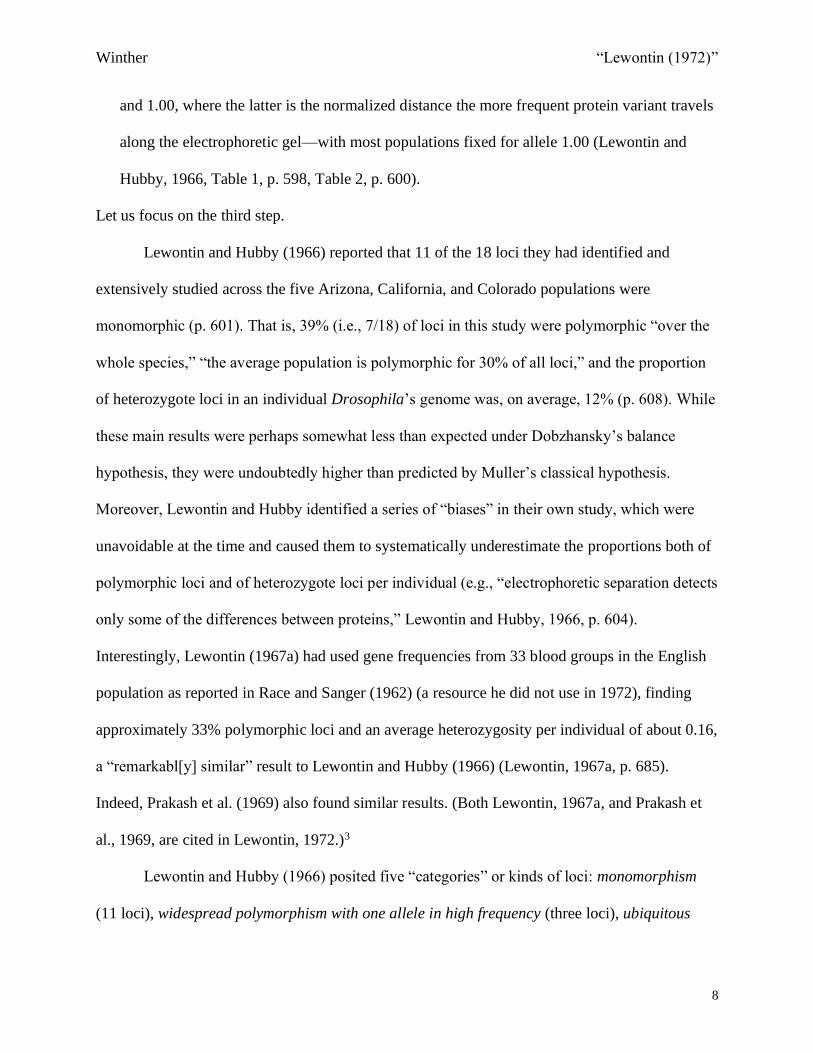
and 1.00, where the latter is the normalized distance the more frequent protein variant travels
along the electrophoretic gel—with most populations fixed for allele 1.00 (Lewontin and
Hubby, 1966, Table 1, p. 598, Table 2, p. 600).
Let us focus on the third step.
Lewontin and Hubby (1966) reported that 11 of the 18 loci they had identified and
extensively studied across the five Arizona, California, and Colorado populations were
monomorphic (p. 601). That is, 39% (i.e., 7/18) of loci in this study were polymorphic “over the
whole species,” “the average population is polymorphic for 30% of all loci,” and the proportion
of heterozygote loci in an individual Drosophila’s genome was, on average, 12% (p. 608). While
these main results were perhaps somewhat less than expected under Dobzhansky’s balance
hypothesis, they were undoubtedly higher than predicted by Muller’s classical hypothesis.
Moreover, Lewontin and Hubby identified a series of “biases” in their own study, which were
unavoidable at the time and caused them to systematically underestimate the proportions both of
polymorphic loci and of heterozygote loci per individual (e.g., “electrophoretic separation detects
only some of the differences between proteins,” Lewontin and Hubby, 1966, p. 604).
Interestingly, Lewontin (1967a) had used gene frequencies from 33 blood groups in the English
population as reported in Race and Sanger (1962) (a resource he did not use in 1972), finding
approximately 33% polymorphic loci and an average heterozygosity per individual of about 0.16,
a “remarkabl[y] similar” result to Lewontin and Hubby (1966) (Lewontin, 1967a, p. 685).
Indeed, Prakash et al. (1969) also found similar results. (Both Lewontin, 1967a, and Prakash et
al., 1969, are cited in Lewontin, 1972.)3
Lewontin and Hubby (1966) posited five “categories” or kinds of loci: monomorphism
(11 loci), widespread polymorphism with one allele in high frequency (three loci), ubiquitous

Winther “Lewontin (1972)”
9
polymorphism with no wild type (three loci), local indigenous polymorphism (one locus), and
local pure races (0 loci). Note that “widespread” implies a lower prevalence than “ubiquitous,”
and “wild type” is a high-frequency and geographically pervasive allele. A “local pure race,”
which was nonexistent in their data set, would correspond to “populations homozygous for one
allele and other populations homozygous for a different one” (Lewontin and Hubby, 1966, p.
602), which would have been very much in line with the classical hypothesis. The names and
relative distributions of these categories resonate with the questions and problematics of
Lewontin (1972).4
But we require one last framing theme, based on an obscure citation to a technical report
out of MIT (Massachusetts Institute of Technology)’s Research Laboratory of Electronics. After
all, Lewontin needed a measure, a statistic, for his analysis.
Statistics and measures of genetic variation
Lewontin required a way to measure the total amount of genetic variation at different levels of
population structure: within local populations, among populations but within continental races,
and among races. Which measure of genetic variation (diversity) should we use, and how should
we assess the relative amount of variation at the three different levels? How should we
“apportion human diversity”?
Standard population genetic theory often starts with the measure of heterozygosity, h: the
total number of heterozygotes of any kind, in a population, at a locus. Lewontin was well aware
of this measure of genetic variation (1972, p. 388; eq. 1.1). (Incidentally, statisticians and
ecologists often refer to this measure as Gini or Gini diversity, per Gini, 1912, cf. Simpson, 1949,
work with which Lewontin possibly was familiar.) However, Lewontin preferred another one:
Winther “Lewontin (1972)”
10
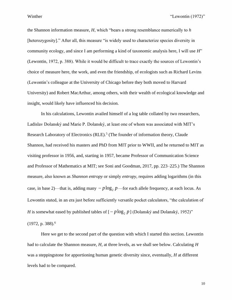
the Shannon information measure, H, which “bears a strong resemblance numerically to h
[heterozygosity].” After all, this measure “is widely used to characterize species diversity in
community ecology, and since I am performing a kind of taxonomic analysis here, I will use H”
(Lewontin, 1972, p. 388). While it would be difficult to trace exactly the sources of Lewontin’s
choice of measure here, the work, and even the friendship, of ecologists such as Richard Levins
(Lewontin’s colleague at the University of Chicago before they both moved to Harvard
University) and Robert MacArthur, among others, with their wealth of ecological knowledge and
insight, would likely have influenced his decision.
In his calculations, Lewontin availed himself of a log table collated by two researchers,
Ladislav Dolanský and Marie P. Dolanský, at least one of whom was associated with MIT’s
Research Laboratory of Electronics (RLE).5 (The founder of information theory, Claude
Shannon, had received his masters and PhD from MIT prior to WWII, and he returned to MIT as
visiting professor in 1956, and, starting in 1957, became Professor of Communication Science
and Professor of Mathematics at MIT; see Soni and Goodman, 2017, pp. 223–225.) The Shannon
measure, also known as Shannon entropy or simply entropy, requires adding logarithms (in this
case, in base 2)—that is, adding many 2 logp p− —for each allele frequency, at each locus. As
Lewontin stated, in an era just before sufficiently versatile pocket calculators, “the calculation of
H is somewhat eased by published tables of [ 2 logp p− ] (Dolanský and Dolanský, 1952)”
(1972, p. 388).6
Here we get to the second part of the question with which I started this section. Lewontin
had to calculate the Shannon measure, H, at three levels, as we shall see below. Calculating H
was a steppingstone for apportioning human genetic diversity since, eventually, H at different
levels had to be compared.

Winther “Lewontin (1972)”
11
Lewontin’s method of comparing H within populations, among populations but within
races, and among races resembles Sewall Wright’s F-statistics.7 Even so, Lewontin’s
bibliography fails us in tracing this influence on Lewontin (1972). Admittedly, Dobzhansky
(1955), contained in Lewontin’s bibliography, cites relevant work by Wright on “panmictic
units” or “demes” to articulate the notion of “Mendelian populations,” which Dobzhansky took
to exist also in Homo sapiens, grounded in “geographic isolation” and “marriage regulation”
(1955, p. 2).
But more generally, and more importantly, Lewontin was familiar with Wright’s rich and
diverse work, including his mathematics of population structure and inbreeding coefficients,
captured in his F-statistics. After all, Wright was a towering figure in population genetics and
had also published with Lewontin’s PhD mentor. Lewontin (1967b) described all of this, and
more. Lewontin concluded a brief review of a 1950 book by Fisher as follows: “That Fisher
could have completed a manuscript on the theory of inbreeding in 1961 without a single mention
of Sewall Wright… bears witness to the power of pride and prejudice” (Lewontin, 1965, p.
1801). Wright’s work attuned geneticists, including Lewontin, to the importance of population
structure and to ways of measuring it.
Bibliographic chasing provides an excellent way to understand Lewontin (1972). The
classical versus balance debate framed his understanding of what was at stake in detecting
genetic variation in a variety of species, including Homo sapiens. And Lewontin was profoundly
sensitive to the centrality of detecting genetic variation at the molecular level, as attested to by
his work with Jack Hubby.
How do we use molecular genetic data to apportion diversity? We require a measure and
a method of partitioning genetic variation. The Shannon measure—fed into an F-statistics-like

Winther “Lewontin (1972)”
12
apportionment of human diversity—was the last mathematical ingredient Lewontin deployed to
answer what, at one point at least in Lewontin (1972), he took to be his “question”: “How much
of human diversity between populations is accounted for by more or less conventional racial
classification?” (p. 386). The short answer? Not much, something like 6.3% [sic]. The longer
answer? Let us revisit Lewontin’s classic article using our three framing themes, addressing each
section in turn.
“Introduction”
Lewontin (1972) starts by discussing the “nodal” nature of variation. That is, “individuals fall in
clusters in the space of phenotypic description.” If we imagine an abstract phenotypic space—
sometimes called a morphospace—with each dimension being a particular phenotypic character
or aggregate set of characters, and each organism is a point in this space, then the organisms of a
species are not evenly distributed throughout this space. Instead, Lewontin admits that there are
three different levels of nodal or clustered variation in Homo sapiens: demes or populations,
races, and our species as a whole. He also suggests that for many, but not all, “post-Darwinians,”
such multilevel nodal structure is a necessary “outcome of an evolutionary process” that takes
genetic variation as its fuel (Lewontin, 1972, p. 381).
Lewontin (1972) can be interpreted as asking the following question: To what extent are
such nodes or groups, in particular human demes (populations) or human races, real? Are such
groups indicative of significant structuring of genetic variation, or are they imposed and reified,
based on our perceptual biases and on classificatory expectations and norms in colonialist and
racist societies?
In a nutshell, are races genetically real?

Winther “Lewontin (1972)”
13
Our first two framing themes help us here. Start with the classical versus balance
hypotheses. According to the classical view, “most men were homozygous for wild-type genes at
virtually all their loci,” such that “the obvious genetical differences in morphological and
physiological characters between races are a major component of the total variation within the
species” (Lewontin, 1972, p. 381). Muller held that different populations and different races (in
organisms in general, not just humans) had been under a long process of selection, leaving most
(if not all) loci fixed, that is, homozygous. Since the alleles fixed at particular loci differ among
populations and among races, most (if not all) genetic variation is among populations or races,
rather than within populations. In contrast, according to the balance view, attributed by Lewontin
to Dobzhansky (1955), “heterozygosity is the rule in sexually reproducing species,” such “that
population and racial variations are likely to be less significant in the total species variation”
(Lewontin, 1972, p. 382). The difference is immense—populations and races would be
genetically real under the classical view, but according to the balance view, they would be mere
cognitive or social (or both) epiphenomena or reifications.
To be precise, and especially for humans, the classical hypothesis of H. J. Muller was
committed to something like the following three positions (Lewontin, 1972, pp. 381–382):
1. Within a species, there are real phenotypic nodes or classes or groups or clusters of organisms,
at populational and racial levels.
2. Each phenotypic node is associated with a certain set of alleles at certain loci; these alleles
tend to be fixed differently in different nodes.
3. Such fixed loci are representative of the clear majority of loci in the different nodes or groups
since all loci have been subject to the strong hand of directional selection.

Winther “Lewontin (1972)”
14
Interestingly, Lewontin accepted the bulk of the first two positions. Later in his article, he
defends “the undoubted existence of such [racial] nodes in the taxonomic space,” insisting that
no one would confuse a Papuan aboriginal with any South American Indian, yet no one can
give an objective criterion for where a dividing line should be drawn in the continuum from
South American Indians through Polynesians, Micronesians, Melanesians, to Papuans.
(Lewontin, 1972, p. 385)
Recall also that he acknowledged that there were “obvious genetical differences” for certain
characters between races (Lewontin, 1972, p. 381). Indeed, Lewontin did not need to accept or
insist on either the ephemerality or subjectivity of populational or racial phenotypic nodes [i.e.,
deny (1)], or the non-existence, or predictive or explanatory weakness, of simple, one-to-one
gene-character (or genotype–phenotype) mappings [i.e., deny (2); although he did deny the
absolute fixation of alleles], to make his overall point that especially genetic races are illusions.
Rather, Lewontin vehemently opposed the classical view regarding position (3)—that the
loci underlying the nodal phenotypes were representative of the genome as a whole. Without the
check of the “objective quantification” of human genetic variation (Lewontin, 1972, p. 382), the
clear cognitive and social biases deploying “obvious and well differentiated stereotypes” (p.
385), and emphasizing intergroup (i.e., interpopulational, interracial) as opposed to intragroup
variation, at both the phenotypic and genotypic levels, could run rampant. We tend to posit
populations, and especially races, based on “those characters to which human perceptions are
most finely tuned (nose, lip and eye shapes, skin color, hair form, and quantity), precisely
because they are the characters that men ordinarily use to distinguish individuals” (p. 382). This
bias belies the third classical hypothesis position that loci informative of populational and,
especially racial, classification (i.e., loci with extreme allele frequency differences among
Winther “Lewontin (1972)”
15
populations, and among races, ideally fixed in different ways in different populations and races)
were representative of all loci. Nevertheless, while Lewontin (1972) is a clear argument against
the third position, Lewontin actually accepts very much here with respect to the classical
hypothesis—more than we would expect and more than he accepted later in his career.
The objective quantification of genetic variation and diversity lies in our second framing
theme, the molecularization of genetics. Lewontin referred both to the methods and the results of
“protein electrophoresis” (reviewed above) and “immunological techniques,” which permit the
“direct” and “objective” assessment and evaluation of genetic diversity, per locus, among human
individuals and groups at various levels of population structure. Citing a number of studies using
“objective techniques” and “older information on the distribution of human blood group genes,”
Lewontin argues that it is possible to estimate the relative amount of intragroup (or intranode)
versus intergroup (internode) genetic variation or diversity in humans and thus to provide a “firm
quantitative basis” to claims about the genetic reality of human racial groups (Lewontin, 1972,
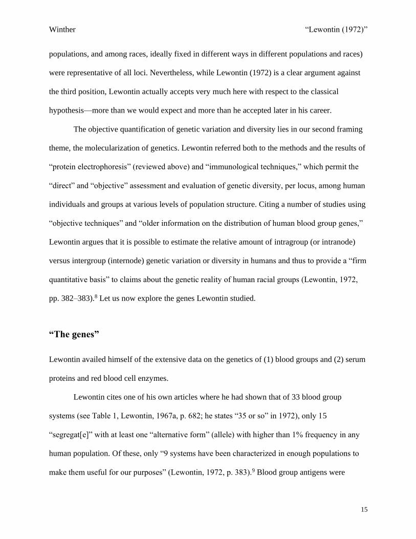
pp. 382–383).8 Let us now explore the genes Lewontin studied.
“The genes”
Lewontin availed himself of the extensive data on the genetics of (1) blood groups and (2) serum
proteins and red blood cell enzymes.
Lewontin cites one of his own articles where he had shown that of 33 blood group
systems (see Table 1, Lewontin, 1967a, p. 682; he states “35 or so” in 1972), only 15
“segregat[e]” with at least one “alternative form” (allele) with higher than 1% frequency in any
human population. Of these, only “9 systems have been characterized in enough populations to
make them useful for our purposes” (Lewontin, 1972, p. 383).9 Blood group antigens were

Winther “Lewontin (1972)”
16
detected by immunological techniques, their phenotypic frequencies in different populations
surveyed, and their genotypic and allele frequencies inferred and calculated. Calculations
followed assumptions about the genetic behavior of each blood group (e.g., gene and allele
number, complete or incomplete dominance and codominance) and about Hardy–Weinberg
equilibrium.
As his sources for blood group information, Lewontin cites Mourant (1954), Mourant et
al. (1958), and Boyd (1950) (1972, p. 383). While he never states the specific tables or pages he
used in these books, it is clear that he relied on their data tables with direct allele frequency
information, and that he also sometimes inferred allele frequencies from phenotypic data, also
given in tables (e.g., Blackfoot Indians for Kidd, Mourant, 1954, Table 39, p. 410,10 and the
entire Lewis data set). Scouring these references reveals that most allele frequency data were
taken from Mourant (1954). By my count, data for six of the nine blood groups were exclusively
from this source (Table 1.1). Titles of Mourant’s Chapters 2–6 name all nine groups (e.g.,
Chapter 6: “The P, Lutheran, Kell, Duffy, Kidd, and Other Systems,” p. v). However, ABO allele
frequency data were almost certainly also taken from Mourant et al. (1958); it’s unclear why else
Lewontin would cite that source, which only contains extensive amounts of ABO data. It is
difficult to determine which populations Lewontin sampled from the many available to him in
very long ABO tables in the three references. One piece of evidence that he used Boyd (1950), at
least for ABO, is that in Table 23, p. 223, Boyd gives ABO data for Shoshone in Wyoming, a
group mentioned in Lewontin’s Table 2 (my Table 1.2), but not otherwise presented, as far as I
can tell, in any other relevant table for the other 16 genes. Boyd (1950) only offered useful allele
frequency tables for ABO, MNS, and Rh (Table 1.1).11
Winther “Lewontin (1972)”
17
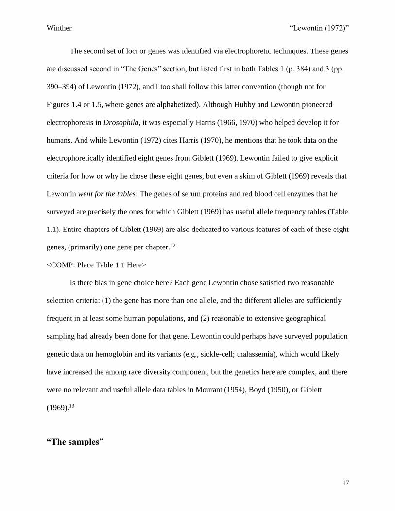
The second set of loci or genes was identified via electrophoretic techniques. These genes
are discussed second in “The Genes” section, but listed first in both Tables 1 (p. 384) and 3 (pp.
390–394) of Lewontin (1972), and I too shall follow this latter convention (though not for
Figures 1.4 or 1.5, where genes are alphabetized). Although Hubby and Lewontin pioneered
electrophoresis in Drosophila, it was especially Harris (1966, 1970) who helped develop it for
humans. And while Lewontin (1972) cites Harris (1970), he mentions that he took data on the
electrophoretically identified eight genes from Giblett (1969). Lewontin failed to give explicit
criteria for how or why he chose these eight genes, but even a skim of Giblett (1969) reveals that
Lewontin went for the tables: The genes of serum proteins and red blood cell enzymes that he
surveyed are precisely the ones for which Giblett (1969) has useful allele frequency tables (Table
1.1). Entire chapters of Giblett (1969) are also dedicated to various features of each of these eight
genes, (primarily) one gene per chapter.12
<COMP: Place Table 1.1 Here>
Is there bias in gene choice here? Each gene Lewontin chose satisfied two reasonable
selection criteria: (1) the gene has more than one allele, and the different alleles are sufficiently
frequent in at least some human populations, and (2) reasonable to extensive geographical
sampling had already been done for that gene. Lewontin could perhaps have surveyed population
genetic data on hemoglobin and its variants (e.g., sickle-cell; thalassemia), which would likely
have increased the among race diversity component, but the genetics here are complex, and there
were no relevant and useful allele data tables in Mourant (1954), Boyd (1950), or Giblett
(1969).13
“The samples”
Winther “Lewontin (1972)”
18
In trying to answer whether races are genetically real—whether racial classification has any
statistical, genetic, or scientific validity—Lewontin faced the colossal task of synthesizing a vast
amount of data from many human populations. He employed a seven-race classification (Table
1.2), listing the populations he drew upon. It is not always easy to determine which exact
populations he used, however; nor what he did when multiple allele frequencies were indicated
for the same population; nor how he aggregated and averaged the allele frequencies of (sub-
)populations. Before identifying just a few issues solely for the case of haptoglobin, I would like
to tackle two dilemmas directly addressed in Lewontin (1972).
First, he aims for a classification that is “a priori representativ[e] of the range of human
diversity” (Lewontin, 1972, p. 384). But how many populations should one sample, and how
should one weight different populations with (immensely) different numbers of individuals? He
ends up counting each population equally (see eqs. 1.7–1.9) and includes “as much as possible,
equal numbers of African peoples, European nationalities, Oceanian populations, Asian peoples,
and American Indian tribes” (p. 385). (How he names and refers to these populations is itself of
interest, as is the fact that Australian aborigines are not here mentioned.) These choices lead to a
bias toward overestimating both the total human genetic diversity and the among populations
diversity component as opposed to the within populations component (see note 21).
The second methodological problem concerns which racial classification system to start
from. Consider the following: Are Sámi (Lapps) Europeans or East Asians? How African are
African Americans? More generally, should we (1) use “linguistic, historical, cultural, and
morphological” “external” evidence, thus decreasing the among races diversity component by
pouring and lumping genetically distinct populations into the same race? Or should we (2) use
entirely genetic evidence to delineate populations and races, though this “has no end” as every

Winther “Lewontin (1972)”
19
population would have to be made a race? Lewontin opts for something quite close to (1), though
he does make “a few switches based on obvious total genetic divergence” (Lewontin, 1972, p.
386).
<COMP: Place Table 1.2 Here>
Even a partial investigation of just one gene—haptoglobin—brings to light issues with
Lewontin’s analysis. The first cell of Table 3 of Lewontin (1972) states 25 as the number of
European populations from which allele frequencies were gathered for haptoglobin. However, in
counting populations in Giblett’s (1969) Table 2.1, pp. 94–95, only 21 of his European
populations match Lewontin’s Table 2 (my Table 1.2). Lewontin does not list, for example,
Sicilians, Sardinians, Yugoslavians, or Australians in Table 1.2. The allele frequencies of all
Italian groups here are so close it is hard to tell how data abstraction (Winther, 2020, Chapter 3)
was performed. Did he lump Sicilians and Sardinians with Italians or did he simply ignore them?
Similarly, Lewontin asserts the use of 21 African populations (Table 3), but comparing Giblett’s
Table 2.1 to Table 1.2 gives only 19 African populations. Why are the Yoruba and Ibadan, which
are listed under Nigerians in Giblett, 1969, p. 95, not listed in Table 1.2, whereas the other three
Nigerian ethnicities listed by Giblett for haptoglobin are—Fulani, Habe, and Ibo? Are African
Americans (p. 96) included under African here—and should they be? (I counted them as such,
per Table 1.2.) Why are Ethiopians or the Kgalagadi from Giblett’s table not listed in Lewontin’s
Table 2?
There are inordinately many small questions about how Lewontin abstracted from the
data tables to his statistical tables.14 After some checking of the mapping of allele frequencies
from data sources to Lewontin’s Table 3 across many of the genes, I have come to accept that
Lewontin’s data abstraction is roughly accurate, even if there are many outstanding questions
Winther “Lewontin (1972)”
20
and concerns.15 What interests me more, and what I turn to in the last two sections, is the actual
population genetic theory behind the apportionment of human diversity, and the recalculation
of—and discovery of multiple errors in—Lewontin’s Table 3.
“The measure of diversity”
Let us explore how Lewontin actually performed his calculations. This section reviews the logic
of his method, while the subsequent section examines Lewontin’s results.
A thought experiment
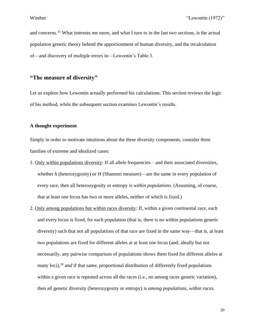
Simply in order to motivate intuitions about the three diversity components, consider three
families of extreme and idealized cases:
1. Only within populations diversity: If all allele frequencies—and their associated diversities,
whether h (heterozygosity) or H (Shannon measure)—are the same in every population of
every race, then all heterozygosity or entropy is within populations. (Assuming, of course,
that at least one locus has two or more alleles, neither of which is fixed.)
2. Only among populations but within races diversity: If, within a given continental race, each
and every locus is fixed, for each population (that is, there is no within populations genetic
diversity) such that not all populations of that race are fixed in the same way—that is, at least
two populations are fixed for different alleles at at least one locus (and, ideally but not
necessarily, any pairwise comparison of populations shows them fixed for different alleles at
many loci),16 and if that same, proportional distribution of differently fixed populations
within a given race is repeated across all the races (i.e., no among races genetic variation),
then all genetic diversity (heterozygosity or entropy) is among populations, within races.
Winther “Lewontin (1972)”
21
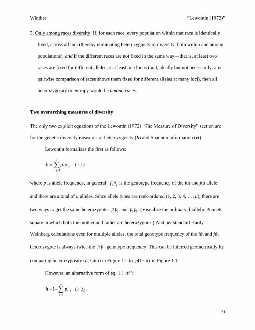
3. Only among races diversity: If, for each race, every population within that race is identically
fixed, across all loci (thereby eliminating heterozygosity or diversity, both within and among
populations), and if the different races are not fixed in the same way—that is, at least two
races are fixed for different alleles at at least one locus (and, ideally but not necessarily, any
pairwise comparison of races shows them fixed for different alleles at many loci), then all
heterozygosity or entropy would be among races.
Two overarching measures of diversity
The only two explicit equations of the Lewontin (1972) “The Measure of Diversity” section are
for the genetic diversity measures of heterozygosity (h) and Shannon information (H).
Lewontin formalizes the first as follows:
, 1
,u
i j
i j
h p p=
= (1.1)
where p is allele frequency, in general; i jp p is the genotype frequency of the ith and jth allele;
and there are a total of u alleles. Since allele types are rank-ordered (1, 2, 3, 4, …, u), there are
two ways to get the same heterozygote: 1 2p p and 2 1p p . (Visualize the ordinary, biallelic Punnett
square in which both the mother and father are heterozygous.) And per standard Hardy–
Weinberg calculations even for multiple alleles, the total genotype frequency of the ith and jth
heterozygote is always twice the i jp p genotype frequency. This can be inferred geometrically by
comparing heterozygosity (h; Gini) in Figure 1.2 to (1 )p p− in Figure 1.1.
However, an alternative form of eq. 1.1 is17:
2
1
1 ,u
i
i
h p=
= − (1.2)

Winther “Lewontin (1972)”
22
where 2
ip is the homozygotic genotype frequency of the ith allele, and there are a total of u
alleles. In general, for multiple alleles, eq. 1.2 is preferred to eq. 1.1, as it is easier for
calculations and for the tracking of genotypes.
Regarding Shannon information, formally, Lewontin writes:
2
1
log ,u
i i
i
H p p=
= − (1.3)
where ip is the frequency of the ith allele, the base of the (binary) logarithm is 2, and there are a
total of u alleles. Above, it was mentioned that Lewontin preferred to use this entropy measure.
<COMP: Place Figure 1.1 Here>
<COMP: Place Figure 1.2 Here>
Diversity is most naturally thought of as a measure of a system’s heterogeneity,
potentially assessed at various hierarchical levels. As justification for the use of these two
measures, Lewontin declaims four criteria that a diversity measure must meet (the criteria names
are mine): (1) minimum diversity criterion: the measure should be at its minimal value, ideally 0,
when there is only one allele in the population (or race or species), or when one allele of several
is fixed; (2) maximum diversity criterion: the measure should be at its maximal value when all
allele frequencies at a locus are equal, that is, when i j k up p p p= = = , and the diversity
should decrease as one or more alleles become rare (and others become common)18; (3) allele
number sensitivity criterion: assuming, for simplicity’s sake, equal allele frequencies, diversity
increases as we increase the number of alleles: “a population with ten [equally frequent] alleles is
obviously more diverse… than a population with two [equally frequent] alleles” (Lewontin,
1972, p. 388); and (4) convexity criterion: we will explore this criterion below. Both h and H

Winther “Lewontin (1972)”
23
satisfy these four conditions, as we can see in Figure 1.2, which represents a minimum diversity
value at 0p = or 1p = and a maximum diversity value at 0.5p = , and is convex.
Six diversity measures
Although he did not explicitly write out any of the following six diversity measures, Lewontin
(1972) effectively calculated each of them for each gene of the 17 genes studied.19
OH , the diversity of a given population:
, 2 ,
1
log ,u
O i m i m
i
H p p=
= − (1.4)
where ,i mp is the frequency of allele i in population m, and u is the total number of alleles at the
particular locus.
raceH , the racially averaged diversity:
, 2 ,
1
log ,u
race i r i r
i
H p p=
= − (1.5)
where ,i rp is the average frequency of the ith allele, within a given race, r, whereas u is the total
number of alleles at the particular locus.20 Lewontin actually calculates the (per allele, per locus)
,i rp by averaging the allele frequencies ,i mp of each population of that race, effectively
“counting each population once” (Lewontin, 1972, p. 389). This diversity value is calculated for
each race independently.
speciesH , the species-averaged diversity:
, 2 ,
1
log ,u
species i s i s
i
H p p=
= − (1.6)

Winther “Lewontin (1972)”
24
where ,i sp is the average frequency of the ith allele, within the entire species, again counting
every single population once, and u is the total number of alleles at a locus. Lewontin actually
calculates the (per allele, per locus) overarching ,i sp as a weighted average in which each race’s
,i rp is weighted according to the number of populations it has ( )rN , out of the total species
population number ( )sN , for that locus.
popH , the average population diversity of a race:
,
1
1,
M
pop O m
m
H HM =
= (1.7)
where ,O mH is the population diversity OH of the mth population of a race, and M is the total
number of populations in the given race. This diversity value is calculated for each race
independently.
popH , the weighted average of every race’s popH :
,
1
1,
R
pop r pop r
rs
H N HN =
= (1.8)
where , pop rH is popH of the rth race, rN is the number of populations in race r (corresponding to
M in eq. 1.7, which often differs for each race), sN is the total number of populations in the
species, and R is the total number of races of the species.
raceH , the weighted average of every race’s raceH :
,
1
1,
R
race r race r
rs
H N HN =
= (1.9)

Winther “Lewontin (1972)”
25
where ,race rH is raceH of the rth race, rN is the number of populations in race r, sN is the total
number of populations in the species, and R is the total number of races of the species.
From these six Shannon information diversity measures, the magic of Lewontin’s
analysis emerges. Here’s how.
Eqs. 1.4–1.6 are explicitly Shannon information measures, using three different allele
frequencies: OH uses allele frequency data of a single population, which is read from the tables
reviewed in the section “The Genes” (this is the only measure of the six not listed in Table 3 of
Lewontin, 1972); raceH uses the original data table allele frequencies within populations,
averaging them over populations, within a race (and is listed for each gene in Table 3 of
Lewontin, 1972); and speciesH averages data table population allele frequencies over the entire
species (and is listed for each gene in Table 3 of Lewontin, 1972). Furthermore, always counting
each population once (i.e., equally), Lewontin calculated three kinds of averages (eqs. 1.7–1.9):
popH , popH , and raceH .
Now, since eqs. 1.4–1.6 use different allele frequencies, three different diversity values
will be produced. Because they are assessed and calculated at different levels, with more
diversity or information (entropy) each time since we average allele frequencies at increasingly
higher levels (viz., other populations within a race; other races), they are broadly independent of
one another. There are metaphorically three degrees of freedom here—constrained by
inequalities given below. This can be understood by observing that popH depends numerically
directly on popH , which depends on OH , whereas raceH is numerically rooted in raceH . Third,
speciesH is not an average of explicit Shannon information diversity measures, but is a Shannon
Winther “Lewontin (1972)”
26
information diversity measure calculated directly from species-level allele frequencies, and is the
highest diversity value of the six.21
The Wahlund effect
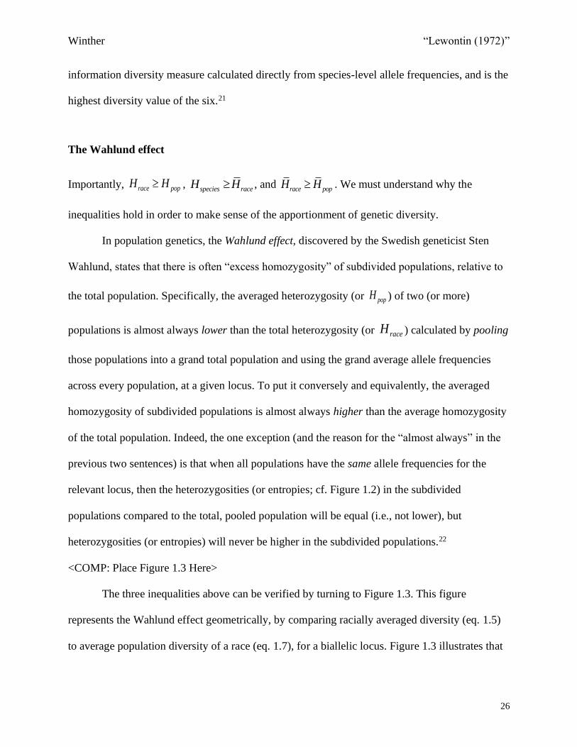
Importantly, race popH H , species raceH H , and race popH H . We must understand why the
inequalities hold in order to make sense of the apportionment of genetic diversity.
In population genetics, the Wahlund effect, discovered by the Swedish geneticist Sten
Wahlund, states that there is often “excess homozygosity” of subdivided populations, relative to
the total population. Specifically, the averaged heterozygosity (or popH ) of two (or more)
populations is almost always lower than the total heterozygosity (or raceH ) calculated by pooling
those populations into a grand total population and using the grand average allele frequencies
across every population, at a given locus. To put it conversely and equivalently, the averaged
homozygosity of subdivided populations is almost always higher than the average homozygosity
of the total population. Indeed, the one exception (and the reason for the “almost always” in the
previous two sentences) is that when all populations have the same allele frequencies for the
relevant locus, then the heterozygosities (or entropies; cf. Figure 1.2) in the subdivided
populations compared to the total, pooled population will be equal (i.e., not lower), but
heterozygosities (or entropies) will never be higher in the subdivided populations.22
<COMP: Place Figure 1.3 Here>
The three inequalities above can be verified by turning to Figure 1.3. This figure
represents the Wahlund effect geometrically, by comparing racially averaged diversity (eq. 1.5)
to average population diversity of a race (eq. 1.7), for a biallelic locus. Figure 1.3 illustrates that
Winther “Lewontin (1972)”
27
raceH will almost always be higher than popH , except when allele frequencies across populations
are identical. In a nutshell: race popH H .23 Differently put, the average allele frequency used to
calculate raceH (or, alternatively, speciesH ) will almost always give a higher diversity than taking
the average of 1OH and 2OH , that is, popH (or, alternatively, raceH ).24
All of this is precisely because of the convexity criterion: “a collection of individuals
made by pooling two populations ought always to be more diverse than the average of their
separate diversities, unless the two populations are identical in composition” (Lewontin, 1972,
388). Observe that the convex diversity function raceH (or, alternatively, speciesH ) almost always
“overshoots” the line connecting the two populations, which must give the (averaged) popH (or,
alternatively, raceH ) exactly at the point on the line cutting allele frequency rp of Figure 1.3,
that is, ,i rp of eq. 1.5 (or, alternatively, ,i sp of eq. 1.6).25 The only time this overshooting does
not hold is when the populations have the same allele frequencies, and the vertical lines collapse
together such that race popH H= (or, alternatively, species raceH H= ).26
If all of this is true for the level depicted in Figure 1.3, it must also be true for measures
averaging those levels, as captured, respectively, by eqs. 1.9 and 1.8. That is, race popH H .
Apportioning diversity at three levels
With this framework in place, Lewontin apportions total, averaged diversity at three distinct
levels. He does this with three explicitly stated equations (pp. 395–396), resonant with Wright’s
F-statistics27:
Winther “Lewontin (1972)”
28
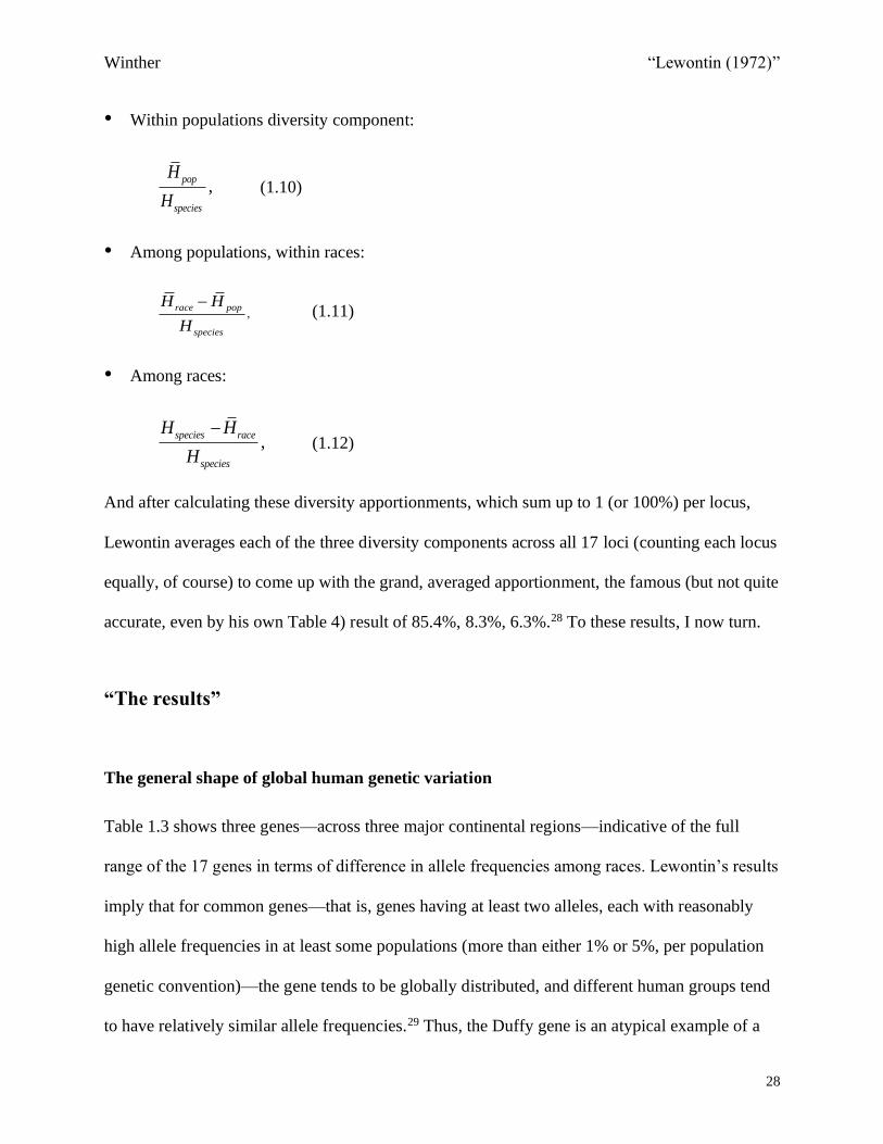
• Within populations diversity component:
,pop
species
H
H (1.10)
• Among populations, within races:
race pop
species
H H
H
−, (1.11)
• Among races:
,species race
species
H H
H
− (1.12)
And after calculating these diversity apportionments, which sum up to 1 (or 100%) per locus,
Lewontin averages each of the three diversity components across all 17 loci (counting each locus
equally, of course) to come up with the grand, averaged apportionment, the famous (but not quite
accurate, even by his own Table 4) result of 85.4%, 8.3%, 6.3%.28 To these results, I now turn.
“The results”
The general shape of global human genetic variation
Table 1.3 shows three genes—across three major continental regions—indicative of the full
range of the 17 genes in terms of difference in allele frequencies among races. Lewontin’s results
imply that for common genes—that is, genes having at least two alleles, each with reasonably
high allele frequencies in at least some populations (more than either 1% or 5%, per population
genetic convention)—the gene tends to be globally distributed, and different human groups tend
to have relatively similar allele frequencies.29 Thus, the Duffy gene is an atypical example of a

Winther “Lewontin (1972)”
29
common gene, as it is more extremely diverged than average.30 Similar to Rh, Duffy has an
among race diversity component of approximately 26%—see eq. 1.12), Table 1.6, and Figures
1.4 and 1.5. In contrast, 6-Phosphogluconate dehydrogenase (6PGD) indicates less variation
among populations than the average common gene. P is beautifully typical of common genes,
showing some variation across continental regions.31
<COMP: Place Table 1.3 Here>
A map key
What do the different values indicated in Lewontin’s (1972) Table 3, pp. 390–394, per gene,
correspond to in the previous section’s formalism?
The top row of N corresponds, for the indicated N of each race, to M (eq. 1.7) or to rN
(eqs. 1.8 and 1.9), and, for the “Total” N of the species, to sN (eqs. 1.8 and 1.9). (I accepted
Lewontin’s assertions of N, and did not question them in my recalculations.)
The second row of p corresponds, for the indicated p of each race, to ,i rp (eq. 1.5),
and for the first entry under the speciesH column,32 to ,i sp (eq. 1.6). (I accepted Lewontin’s
assertions of p , i.e., ,i rp , for each race, and did not question them in my recalculations.)
The last three rows simply correspond, per race, to diversity values that are calculated,
respectively, by eqs. 1.5 and 1.7 and by dividing the latter value by the former. (I accepted
Lewontin’s assertions of popH , i.e., eq. 1.7, per locus per race, and did not question them in my
recalculations.)
Winther “Lewontin (1972)”
30
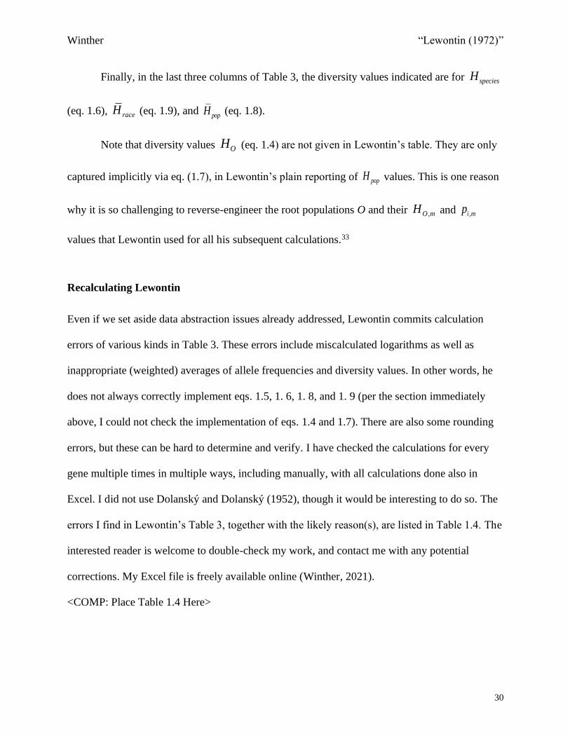
Finally, in the last three columns of Table 3, the diversity values indicated are for speciesH
(eq. 1.6), raceH (eq. 1.9), and popH (eq. 1.8).
Note that diversity values OH (eq. 1.4) are not given in Lewontin’s table. They are only
captured implicitly via eq. (1.7), in Lewontin’s plain reporting of popH values. This is one reason
why it is so challenging to reverse-engineer the root populations O and their ,O mH and ,i mp
values that Lewontin used for all his subsequent calculations.33
Recalculating Lewontin
Even if we set aside data abstraction issues already addressed, Lewontin commits calculation
errors of various kinds in Table 3. These errors include miscalculated logarithms as well as
inappropriate (weighted) averages of allele frequencies and diversity values. In other words, he
does not always correctly implement eqs. 1.5, 1. 6, 1. 8, and 1. 9 (per the section immediately
above, I could not check the implementation of eqs. 1.4 and 1.7). There are also some rounding
errors, but these can be hard to determine and verify. I have checked the calculations for every
gene multiple times in multiple ways, including manually, with all calculations done also in
Excel. I did not use Dolanský and Dolanský (1952), though it would be interesting to do so. The
errors I find in Lewontin’s Table 3, together with the likely reason(s), are listed in Table 1.4. The
interested reader is welcome to double-check my work, and contact me with any potential
corrections. My Excel file is freely available online (Winther, 2021).
<COMP: Place Table 1.4 Here>
Winther “Lewontin (1972)”
31
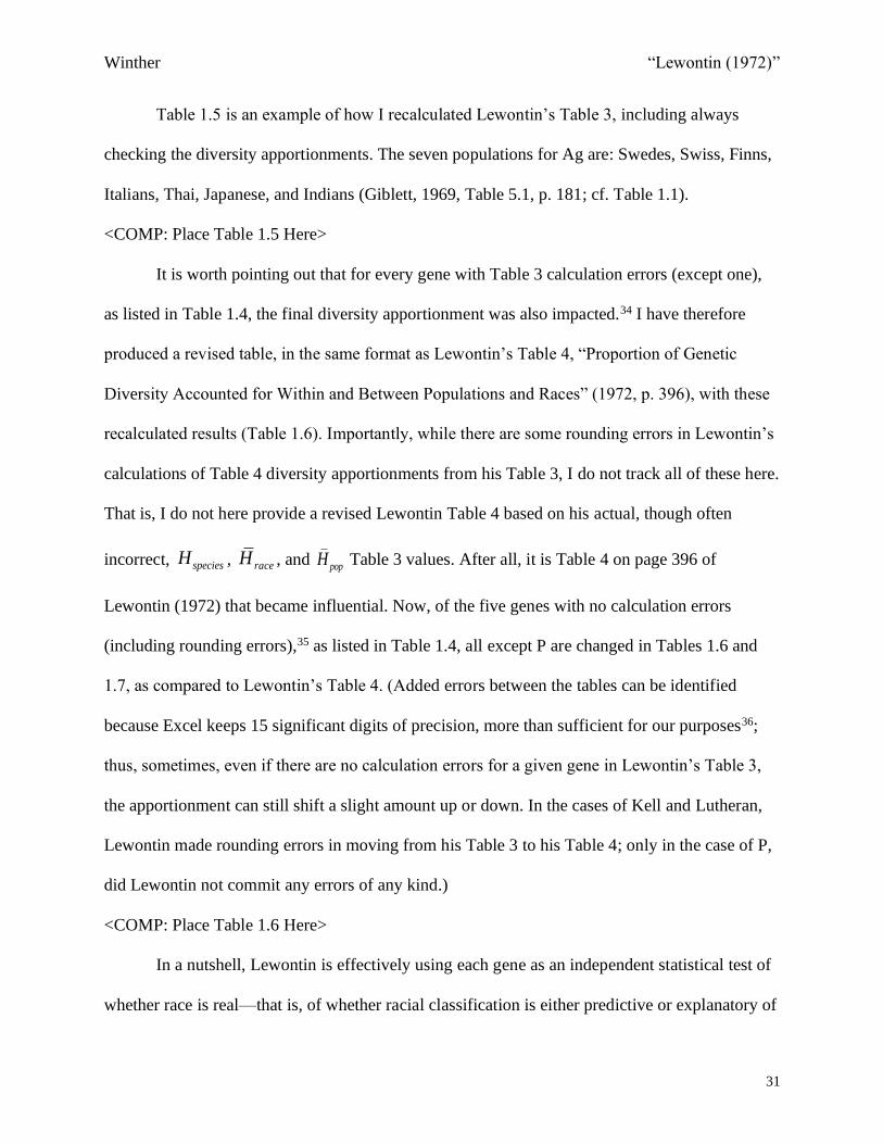
Table 1.5 is an example of how I recalculated Lewontin’s Table 3, including always
checking the diversity apportionments. The seven populations for Ag are: Swedes, Swiss, Finns,
Italians, Thai, Japanese, and Indians (Giblett, 1969, Table 5.1, p. 181; cf. Table 1.1).
<COMP: Place Table 1.5 Here>
It is worth pointing out that for every gene with Table 3 calculation errors (except one),
as listed in Table 1.4, the final diversity apportionment was also impacted.34 I have therefore
produced a revised table, in the same format as Lewontin’s Table 4, “Proportion of Genetic
Diversity Accounted for Within and Between Populations and Races” (1972, p. 396), with these
recalculated results (Table 1.6). Importantly, while there are some rounding errors in Lewontin’s
calculations of Table 4 diversity apportionments from his Table 3, I do not track all of these here.
That is, I do not here provide a revised Lewontin Table 4 based on his actual, though often
incorrect, speciesH , raceH , and popH Table 3 values. After all, it is Table 4 on page 396 of
Lewontin (1972) that became influential. Now, of the five genes with no calculation errors
(including rounding errors),35 as listed in Table 1.4, all except P are changed in Tables 1.6 and
1.7, as compared to Lewontin’s Table 4. (Added errors between the tables can be identified
because Excel keeps 15 significant digits of precision, more than sufficient for our purposes36;
thus, sometimes, even if there are no calculation errors for a given gene in Lewontin’s Table 3,
the apportionment can still shift a slight amount up or down. In the cases of Kell and Lutheran,
Lewontin made rounding errors in moving from his Table 3 to his Table 4; only in the case of P,
did Lewontin not commit any errors of any kind.)
<COMP: Place Table 1.6 Here>
In a nutshell, Lewontin is effectively using each gene as an independent statistical test of
whether race is real—that is, of whether racial classification is either predictive or explanatory of

Winther “Lewontin (1972)”
32
genetic differences among groups (Table 1.6). Lewontin wants to say that it is neither predictive
nor explanatory.
<COMP: Place Table 1.7 Here>
For almost all of the 17 genes, except for P, Lewontin made at least one calculation error
(including rounding errors). Only a few of these errors were serious, and they were not
systematic (Figures 1.4 and 1.5). However, the overstatement (by 0.7%) of the among
populations diversity component and the understatement (by 1.3%) of the among races
components, relative to just his own Table 4, merit further discussion (Table 1.6). Since the
recalculated among populations but within races and among races diversity components are
almost the same—7.1/7.2%—I suggest that we rethink Lewontin’s distribution as properly
86%/7%/7% (Table 1.6). While this result may seem anticlimactic, it may be a better
mnemonic. I, for one, am grateful for having been able to redo all his calculations in order to
ensure that we are getting the calculations right in this area of inquiry, and in the interest of
scientific reproducibility.37
<COMP: Place Figure 1.4 Here>
<COMP: Place Figure 1.5 Here>
Conclusion
Lewontin (1972) deserves to be celebrated as it turns 50. In beginning work on what was
intended to be a short introduction to the piece, its deep multidimensionality became quickly
clear to me: evolutionary theory, statistics, politics, and ethics intertwine. As I started finding
errors in his results, and as I began digging into his concise but illuminating bibliography, I
realized that it would not be a simple matter to introduce this seminal work. I felt I had to
Winther “Lewontin (1972)”
33
describe Lewontin before Lewontin (1972), present the content—explicit as well as implicit—of
the different sections of his article, and carefully check all his calculations and claims. The
resulting chapter is a kind of field guide to Lewontin (1972).
This chapter does not attempt to cover everything. For instance, Lewontin, a Marxist,
mentions on the first page of his article the importance of “long-term changes in socioeconomic
relations” in shaping professional views on “the relative importance and extent of intragroup as
opposed to intergroup variation” (Lewontin, 1972, p. 381, citing Lewontin, 1968), and he also
believes he has shown “racial classification” to be “of virtually no genetic or taxonomic
significance” (Lewontin, 1972, p. 397). More ironically, he accepts race at a phenotypic level, as
we saw above; he is not as judgmentally harsh about the genetic reality of populations qua nodes
or groups as he is about the genetic reality of races qua nodes or groups, although he finds that
their diversity apportionments are commensurable, and even overstates the former diversity
component at the expense of the latter, and two years later publishes a book (Lewontin, 1974)
arguing for the entire genome as a unit of selection—even though in 1972 he unavoidably
averages across loci, thereby losing classificatory information, as so many of the chapters in this
volume, and elsewhere, discuss (e.g., Winther, 2018).38
In addition, there are potential ethical concerns in data collection and management, and in
theoretical calculation, abstraction, and modeling. Almost certainly, there are any number of
such concerns involved in the data collection and management of the thousands of research
papers consulted by Mourant (1954) (e.g., 1716 numbered references, pp. 239–33539), and the
many hundreds referred to by Giblett (1969), in mapping out their rich data tables of allele
frequencies. These important ethical issues have been covered in this volume by Guillermo
Delgado-P, Kelly Happe, and Krystal Tsosie. The extent and exact nature of Lewontin’s

Winther “Lewontin (1972)”
34
culpability in such matters—indirect as it may be—is interesting and should be further
investigated.
I hope I will be forgiven for not discussing these matters here, as they have been
discussed extensively and perhaps exhaustively elsewhere. The particular responsibility of my
chapter is to present, for the first time it would seem, the full flesh and bones of the scientific
background, data, theory, and results of Lewontin (1972). After all, this classic is remarkably
telegraphic. It neither explicitly lists data sources nor explains background population genetic
theory. It is also replete with calculation errors—recall that Lewontin made errors for all genes
except one.
Could I derive Lewontin’s results from his data? Could I replicate and reproduce his
analyses? In the end, his diversity component distribution among the three levels should be
revised to 86%/7%/7%. This is a small correction. While Lewontin’s calculation errors are not
systematic (Figures 1.4 and 1.5), this could not have been known before the recalculations
presented in this chapter, nor could the fact that he overstates the among populations diversity
component while understating the among races diversity component, even by his own Table 4
(Table 1.6). We should also recall that his results have (only) roughly held up to the test of
time.40 Fifty years on from Lewontin (1972), it is important to remember that, in addition to
adulating a great work such as this one, we must also strive to understand and evaluate, on a deep
level, its content.
Acknowledgments

Winther “Lewontin (1972)”
35
Lucas McGranahan copyedited expertly, Amir Najmi was a sounding board for the figures, and
Marie Raffn was an inspiration. Correspondence and occasional conversations over the years
with Richard C. Lewontin have been a gift, as has his ongoing support.
Figure 1.1 Entropy (H) and Gini (h) summand values. The values of the components (summands)
of our two measures, plotted against allele frequency p, for a biallelic locus. (Concept and draft
by Rasmus Grønfeldt Winther; illustrated by Amir Najmi using ggplot2 in R.)
Figure 1.2 Entropy versus Gini diversity. The actual diversity values of Shannon information, H,
and heterozygosity, h, mapped against allele frequency, for a biallelic locus, per, respectively,
eqs (1.3) and (1.1) or (1.2). (Concept and draft by Rasmus Grønfeldt Winther; illustrated by
Amir Najmi using ggplot2 in R.)
Figure 1.3 The Wahlund effect per convexity criterion. Two populations are shown, and diversity
is entropy, that is, the Shannon information measure. 1OH and 2OH are the diversities of the first
and the second population, respectively. Since the locus is biallelic—i.e., the other allele
frequency is simply (1 )p− —and to avoid confusion both about which population’s allele
frequency is being depicted and about the fact that the frequency for the same allele is
represented in both populations, ,i mp is written as 1Op and 2Op for, respectively, the first and
the second population. See text for further archaeology of the figure. (Concept and draft by
Rasmus Grønfeldt Winther; illustrated by Amir Najmi using ggplot2 in R.)
Figure 1.4 Lewontin–Winther bar plots. Bar plots of the three diversity components for each
gene (on the same scale), as presented in Lewontin’s Table 4, p. 396, compared to the true
recalculated values from Table 1.6. Differences are often minimal. (Concept and illustration by
Amir Najmi using ggplot2 in R.)
Winther “Lewontin (1972)”
36
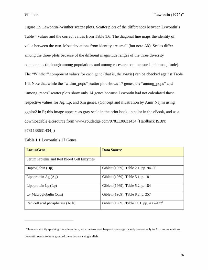
Figure 1.5 Lewontin–Winther scatter plots. Scatter plots of the differences between Lewontin’s
Table 4 values and the correct values from Table 1.6. The diagonal line maps the identity of
value between the two. Most deviations from identity are small (but note Ak). Scales differ
among the three plots because of the different magnitude ranges of the three diversity
components (although among populations and among races are commensurable in magnitude).
The “Winther” component values for each gene (that is, the x-axis) can be checked against Table
1.6. Note that while the “within_pops” scatter plot shows 17 genes, the “among_pops” and
“among_races” scatter plots show only 14 genes because Lewontin had not calculated those
respective values for Ag, Lp, and Xm genes. (Concept and illustration by Amir Najmi using
ggplot2 in R; this image appears as gray scale in the print book, in color in the eBook, and as a
downloadable eResource from www.routledge.com/9781138631434 [Hardback ISBN:
9781138631434].)
Table 1.1 Lewontin’s 17 Genes
Locus/Gene Data Source
Serum Proteins and Red Blood Cell Enzymes
Haptoglobin (Hp) Giblett (1969), Table 2.1, pp. 94–98
Lipoprotein Ag (Ag) Giblett (1969), Table 5.1, p. 181
Lipoprotein Lp (Lp) Giblett (1969), Table 5.2, p. 184
2 Macroglobulin (Xm) Giblett (1969), Table 8.2, p. 257
Red cell acid phosphatase (APh) Giblett (1969), Table 11.1, pp. 436–4371
1 There are strictly speaking five alleles here, with the two least frequent ones significantly present only in African populations.
Lewontin seems to have grouped these two as a single allele.
Winther “Lewontin (1972)”
37
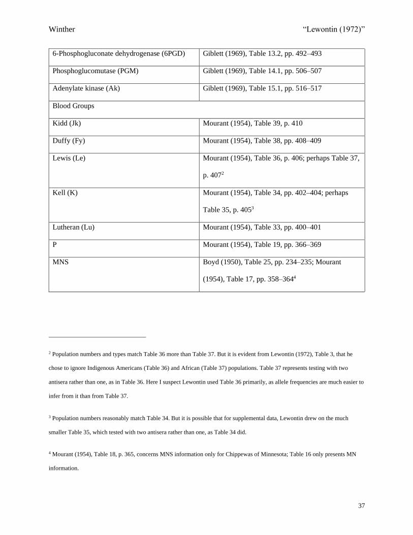
6-Phosphogluconate dehydrogenase (6PGD) Giblett (1969), Table 13.2, pp. 492–493
Phosphoglucomutase (PGM) Giblett (1969), Table 14.1, pp. 506–507
Adenylate kinase (Ak) Giblett (1969), Table 15.1, pp. 516–517
Blood Groups
Kidd (Jk) Mourant (1954), Table 39, p. 410
Duffy (Fy) Mourant (1954), Table 38, pp. 408–409
Lewis (Le) Mourant (1954), Table 36, p. 406; perhaps Table 37,
p. 4072
Kell (K) Mourant (1954), Table 34, pp. 402–404; perhaps
Table 35, p. 4053
Lutheran (Lu) Mourant (1954), Table 33, pp. 400–401
P Mourant (1954), Table 19, pp. 366–369
MNS Boyd (1950), Table 25, pp. 234–235; Mourant
(1954), Table 17, pp. 358–3644
2 Population numbers and types match Table 36 more than Table 37. But it is evident from Lewontin (1972), Table 3, that he
chose to ignore Indigenous Americans (Table 36) and African (Table 37) populations. Table 37 represents testing with two
antisera rather than one, as in Table 36. Here I suspect Lewontin used Table 36 primarily, as allele frequencies are much easier to
infer from it than from Table 37.
3 Population numbers reasonably match Table 34. But it is possible that for supplemental data, Lewontin drew on the much
smaller Table 35, which tested with two antisera rather than one, as Table 34 did.
4 Mourant (1954), Table 18, p. 365, concerns MNS information only for Chippewas of Minnesota; Table 16 only presents MN
information.
Winther “Lewontin (1972)”
38
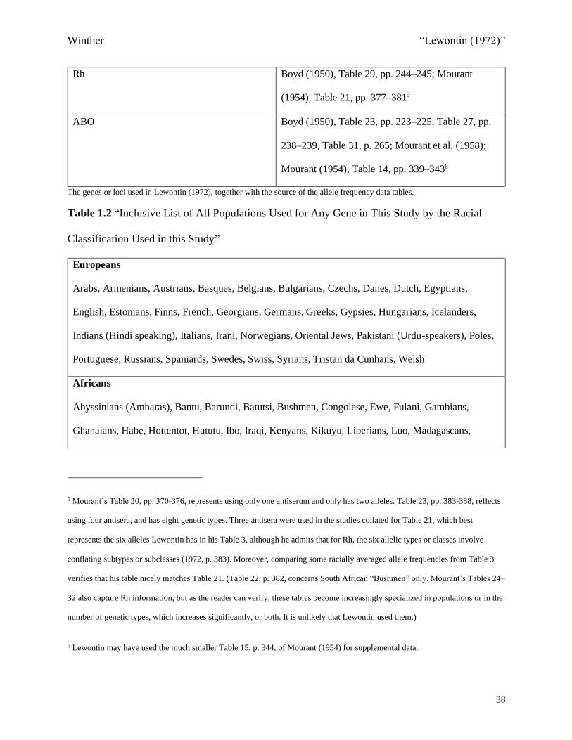
Rh Boyd (1950), Table 29, pp. 244–245; Mourant
(1954), Table 21, pp. 377–3815
ABO Boyd (1950), Table 23, pp. 223–225, Table 27, pp.
238–239, Table 31, p. 265; Mourant et al. (1958);
Mourant (1954), Table 14, pp. 339–3436
The genes or loci used in Lewontin (1972), together with the source of the allele frequency data tables.
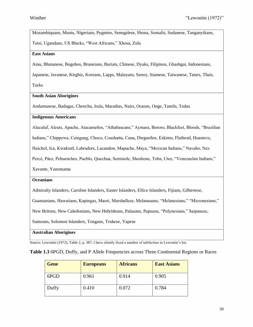
Table 1.2 “Inclusive List of All Populations Used for Any Gene in This Study by the Racial
Classification Used in this Study”
Europeans
Arabs, Armenians, Austrians, Basques, Belgians, Bulgarians, Czechs, Danes, Dutch, Egyptians,
English, Estonians, Finns, French, Georgians, Germans, Greeks, Gypsies, Hungarians, Icelanders,
Indians (Hindi speaking), Italians, Irani, Norwegians, Oriental Jews, Pakistani (Urdu-speakers), Poles,
Portuguese, Russians, Spaniards, Swedes, Swiss, Syrians, Tristan da Cunhans, Welsh
Africans
Abyssinians (Amharas), Bantu, Barundi, Batutsi, Bushmen, Congolese, Ewe, Fulani, Gambians,
Ghanaians, Habe, Hottentot, Hututu, Ibo, Iraqi, Kenyans, Kikuyu, Liberians, Luo, Madagascans,
5 Mourant’s Table 20, pp. 370-376, represents using only one antiserum and only has two alleles. Table 23, pp. 383-388, reflects
using four antisera, and has eight genetic types. Three antisera were used in the studies collated for Table 21, which best
represents the six alleles Lewontin has in his Table 3, although he admits that for Rh, the six allelic types or classes involve
conflating subtypes or subclasses (1972, p. 383). Moreover, comparing some racially averaged allele frequencies from Table 3
verifies that his table nicely matches Table 21. (Table 22, p. 382, concerns South African “Bushmen” only. Mourant’s Tables 24–
32 also capture Rh information, but as the reader can verify, these tables become increasingly specialized in populations or in the
number of genetic types, which increases significantly, or both. It is unlikely that Lewontin used them.)
6 Lewontin may have used the much smaller Table 15, p. 344, of Mourant (1954) for supplemental data.
Winther “Lewontin (1972)”
39
Mozambiquans, Msutu, Nigerians, Pygmies, Senegalese, Shona, Somalis, Sudanese, Tanganyikans,
Tutsi, Ugandans, US Blacks, “West Africans,” Xhosa, Zulu
East Asians
Ainu, Bhutanese, Bogobos, Bruneians, Buriats, Chinese, Dyaks, Filipinos, Ghashgai, Indonesians,
Japanese, Javanese, Kirghiz, Koreans, Lapps, Malayans, Senoy, Siamese, Taiwanese, Tatars, Thais,
Turks
South Asian Aborigines
Andamanese, Badagas, Chenchu, Irula, Marathas, Nairs, Oraons, Onge, Tamils, Todas
Indigenous Americans
Alacaluf, Aleuts, Apache, Atacameños, “Athabascans,” Aymara, Bororo, Blackfeet, Bloods, “Brazilian
Indians,” Chippewa, Caingang, Choco, Coushatta, Cuna, Diegueños, Eskimo, Flathead, Huasteco,
Huichol, Ica, Kwakiutl, Labradors, Lacandon, Mapuche, Maya, “Mexican Indians,” Navaho, Nez
Percé, Páez, Pehuenches, Pueblo, Quechua, Seminole, Shoshone, Toba, Utes, “Venezuelan Indians,”
Xavante, Yanomama
Oceanians
Admiralty Islanders, Caroline Islanders, Easter Islanders, Ellice Islanders, Fijians, Gilbertese,
Guamanians, Hawaiians, Kapingas, Maori, Marshallese, Melanauans, “Melanesians,” “Micronesians,”
New Britons, New Caledonians, New Hebrideans, Palauans, Papuans, “Polynesians,” Saipanese,
Samoans, Solomon Islanders, Tongans, Trukese, Yapese
Australian Aborigines
Source: Lewontin (1972), Table 2, p. 387; I have silently fixed a number of infelicities in Lewontin’s list.
Table 1.3 6PGD, Duffy, and P Allele Frequencies across Three Continental Regions or Races
Gene Europeans Africans East Asians
6PGD 0.961 0.914 0.905
Duffy 0.410 0.072 0.784
Winther “Lewontin (1972)”
40
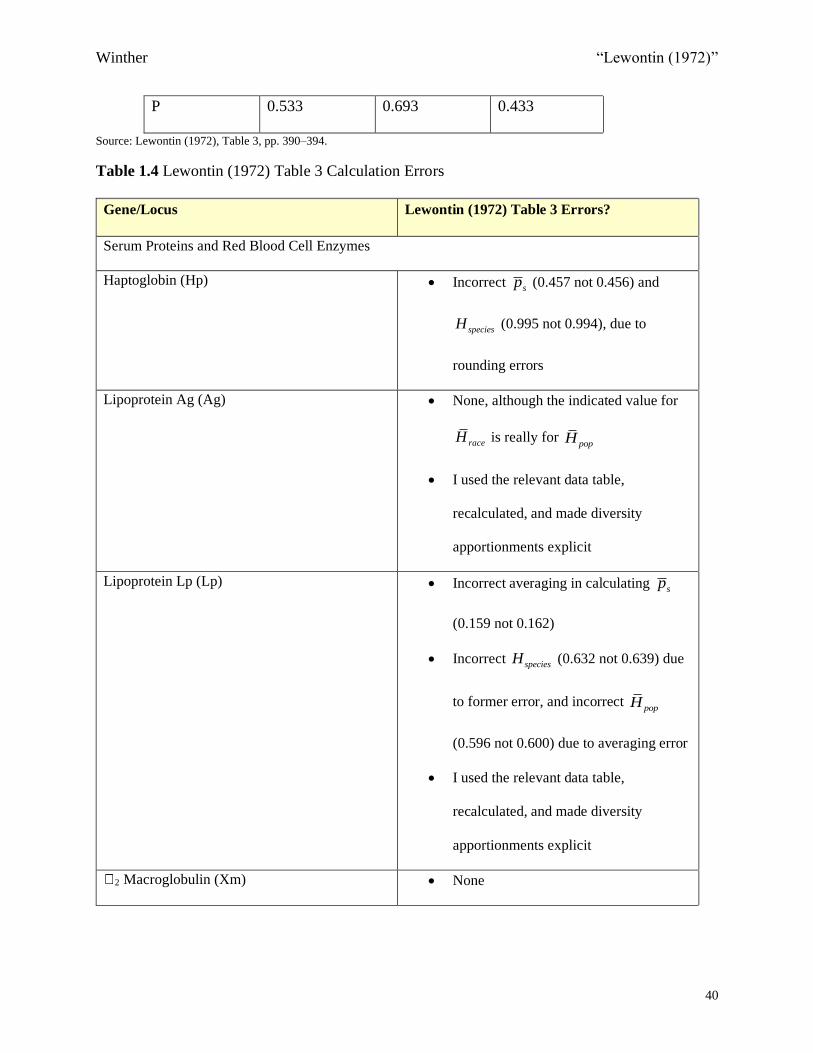
P 0.533 0.693 0.433
Source: Lewontin (1972), Table 3, pp. 390–394.
Table 1.4 Lewontin (1972) Table 3 Calculation Errors
Gene/Locus Lewontin (1972) Table 3 Errors?
Serum Proteins and Red Blood Cell Enzymes
Haptoglobin (Hp) • Incorrect sp (0.457 not 0.456) and
speciesH (0.995 not 0.994), due to
rounding errors
Lipoprotein Ag (Ag) • None, although the indicated value for
raceH is really for popH
• I used the relevant data table,
recalculated, and made diversity
apportionments explicit
Lipoprotein Lp (Lp) • Incorrect averaging in calculating sp
(0.159 not 0.162)
• Incorrect speciesH (0.632 not 0.639) due
to former error, and incorrect popH
(0.596 not 0.600) due to averaging error
• I used the relevant data table,
recalculated, and made diversity
apportionments explicit
2 Macroglobulin (Xm) • None

Winther “Lewontin (1972)”
41
• I used the relevant data table,
recalculated, and made diversity
apportionments explicit
Red Cell Acid Phosphatase (APh) • Incorrect raceH (0.976 not 0.977) and
popH (0.918 not 0.917), due to rounding
errors
• Incorrect 2,sp (0.682 not 0.683) and
4,sp (0.002 not 0.001), both likely
rounding errors
• Incorrect speciesH (0.999 not 0.989) due
to logarithm or rounding errors, or both7
6-Phosphogluconate dehydrogenase (6PGD) • Incorrect popH (0.287 not 0.286) due to
a rounding error
Phosphoglucomutase (PGM) • Incorrect speciesH (0.759 not 0.758) due
to a rounding error
7 By “logarithm error,” I mean any error Lewontin might have made in reading or calculating from the values listed in Dolanský
and Dolanský (1952). They list the values of p for calculating binary or base two logarithms to three decimal figures, and the
actual logarithmic values to six decimal figures. Interestingly, and likely because he followed this logarithm table, Lewontin
presented all allele frequencies to the nearest thousandth. (Every diversity measure and subsequent diversity apportionment was
also rounded to the nearest thousandth by Lewontin.) Depending on the gene, Gibblett (1969) presented allele frequency data to
the nearest hundredth or thousandth, and Mourant (1954) generally to the nearest ten thousandth.
Winther “Lewontin (1972)”
42
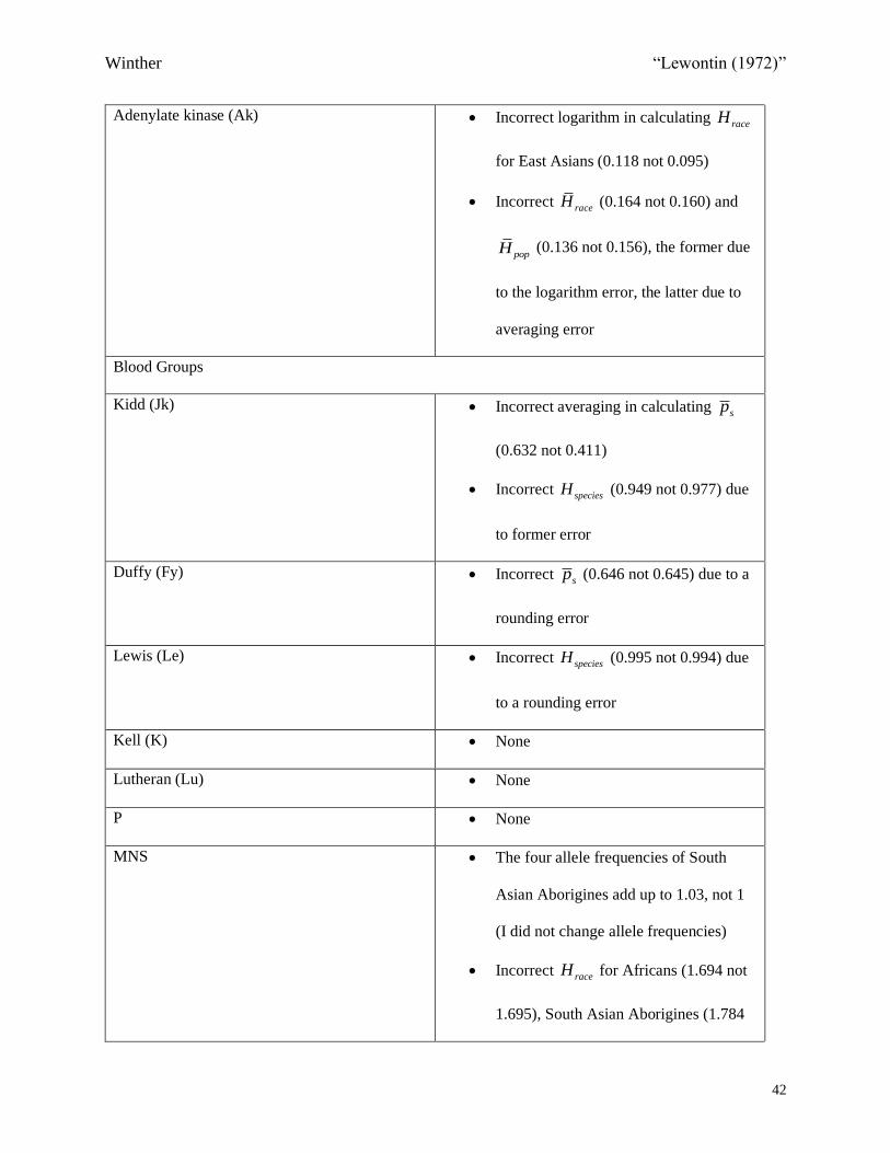
Adenylate kinase (Ak) • Incorrect logarithm in calculating raceH
for East Asians (0.118 not 0.095)
• Incorrect raceH (0.164 not 0.160) and
popH (0.136 not 0.156), the former due
to the logarithm error, the latter due to
averaging error
Blood Groups
Kidd (Jk) • Incorrect averaging in calculating sp
(0.632 not 0.411)
• Incorrect speciesH (0.949 not 0.977) due
to former error
Duffy (Fy) • Incorrect sp (0.646 not 0.645) due to a
rounding error
Lewis (Le) • Incorrect speciesH (0.995 not 0.994) due
to a rounding error
Kell (K) • None
Lutheran (Lu) • None
P • None
MNS • The four allele frequencies of South
Asian Aborigines add up to 1.03, not 1
(I did not change allele frequencies)
• Incorrect raceH for Africans (1.694 not
1.695), South Asian Aborigines (1.784

Winther “Lewontin (1972)”
43
not 1.785), and Indigenous Americans
(1.534 not 1.609), due to logarithm or
rounding errors, or both
• Incorrect 2,sp (0.421 not 0.420) and
4,sp (0.354 not 0.353), both likely
rounding errors
• Incorrect raceH (1.655 not 1.663) and
popH (1.581 not 1.591), the former due
to prior raceH errors, the latter due to
averaging error
Rh • The six allele frequencies add up to 1
only for Oceanians and Australian
Aborigines (I did not change allele
frequencies)
• Incorrect averaging in calculating 1,sp
(0.517 not 0.518), 3,sp (0.147 not
0.148), and 5,sp (0.165 not 0.166),
likely rounding errors
• Incorrect raceH for Europeans (1.765
not 1.763), Indigenous Americans (1.51
not 1.509), and Australian Aborigines
(1.601 not 1.600), due to logarithm or
rounding errors, or both
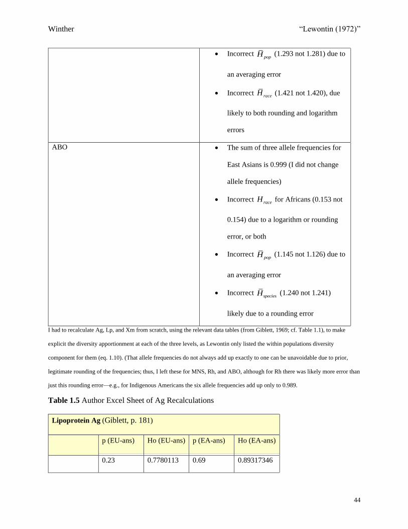
Winther “Lewontin (1972)”
44
• Incorrect popH (1.293 not 1.281) due to
an averaging error
• Incorrect raceH (1.421 not 1.420), due
likely to both rounding and logarithm
errors
ABO • The sum of three allele frequencies for
East Asians is 0.999 (I did not change
allele frequencies)
• Incorrect raceH for Africans (0.153 not
0.154) due to a logarithm or rounding
error, or both
• Incorrect popH (1.145 not 1.126) due to
an averaging error
• Incorrect speciesH (1.240 not 1.241)
likely due to a rounding error
I had to recalculate Ag, Lp, and Xm from scratch, using the relevant data tables (from Giblett, 1969; cf. Table 1.1), to make
explicit the diversity apportionment at each of the three levels, as Lewontin only listed the within populations diversity
component for them (eq. 1.10). (That allele frequencies do not always add up exactly to one can be unavoidable due to prior,
legitimate rounding of the frequencies; thus, I left these for MNS, Rh, and ABO, although for Rh there was likely more error than
just this rounding error—e.g., for Indigenous Americans the six allele frequencies add up only to 0.989.
Table 1.5 Author Excel Sheet of Ag Recalculations
Lipoprotein Ag (Giblett, p. 181)
p (EU-ans) Ho (EU-ans) p (EA-ans) Ho (EA-ans)
0.23 0.7780113 0.69 0.89317346

Winther “Lewontin (1972)”
45
0.24 0.79504028 0.73 0.84146464
0.31 0.89317346 0.74 0.82674637
0.23 0.7780113
N 4
3
Hpop
0.81105909
0.85379482
Hpop-bar
0.8293744
p-bar (race) 0.2525
0.720
H race 0.81521654
0.85545081
Hrace-bar 0.8324598
p-bar
(species)
0.45285714
Hspecies 0.99357783
w/in pops
0.83473521
Among
pops/within
race
0.00310534
Among races
0.16215945
Source of data: Giblett (1969), 5.1, p. 181; cf. Table 1.1 above.
“EU-ans”: European populations; “EA-ans”: East Asian populations. Equations are embedded in the cells.
Table 1.6 The True Genetic Diversity Apportionment
Within Pops Among
Pops
Among
Races
Hp 0.893 0.050 0.057
Ag 0.835 0.003 0.162
Lp 0.942 0.025 0.033
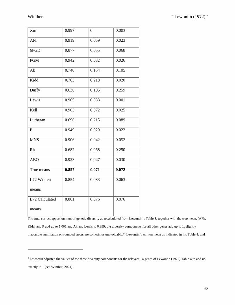
Winther “Lewontin (1972)”
46
Xm 0.997 0 0.003
APh 0.919 0.059 0.023
6PGD 0.877 0.055 0.068
PGM 0.942 0.032 0.026
Ak 0.740 0.154 0.105
Kidd 0.763 0.218 0.020
Duffy 0.636 0.105 0.259
Lewis 0.965 0.033 0.001
Kell 0.903 0.072 0.025
Lutheran 0.696 0.215 0.089
P 0.949 0.029 0.022
MNS 0.906 0.042 0.052
Rh 0.682 0.068 0.250
ABO 0.923 0.047 0.030
True means 0.857 0.071 0.072
L72 Written
means
0.854 0.083 0.063
L72 Calculated
means
0.861 0.076 0.076
The true, correct apportionment of genetic diversity as recalculated from Lewontin’s Table 3, together with the true mean. (APh,
Kidd, and P add up to 1.001 and Ak and Lewis to 0.999; the diversity components for all other genes add up to 1; slightly
inaccurate summation on rounded errors are sometimes unavoidable.8) Lewontin’s written mean as indicated in his Table 4, and
8 Lewontin adjusted the values of the three diversity components for the relevant 14 genes of Lewontin (1972) Table 4 to add up
exactly to 1 (see Winther, 2021).
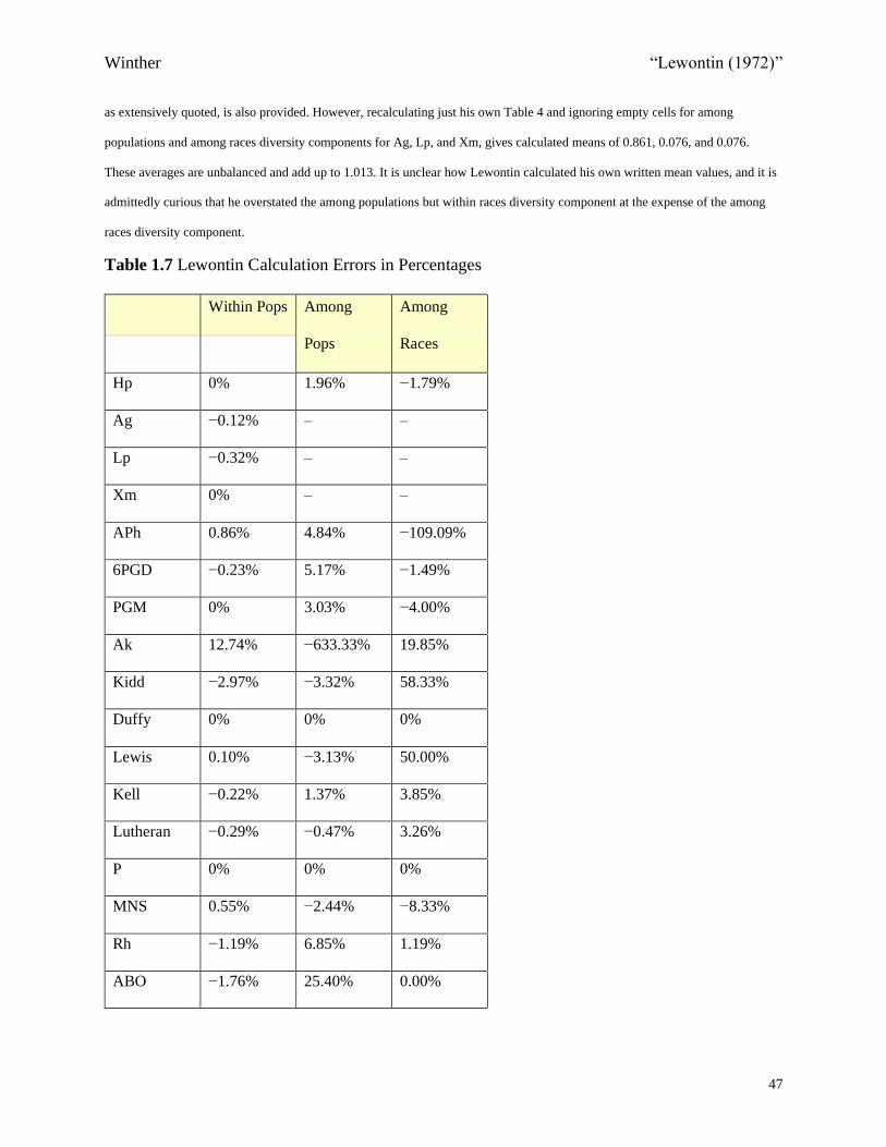
Winther “Lewontin (1972)”
47
as extensively quoted, is also provided. However, recalculating just his own Table 4 and ignoring empty cells for among
populations and among races diversity components for Ag, Lp, and Xm, gives calculated means of 0.861, 0.076, and 0.076.
These averages are unbalanced and add up to 1.013. It is unclear how Lewontin calculated his own written mean values, and it is
admittedly curious that he overstated the among populations but within races diversity component at the expense of the among
races diversity component.
Table 1.7 Lewontin Calculation Errors in Percentages
Within Pops Among
Pops
Among
Races
Hp 0% 1.96% −1.79%
Ag −0.12% – –
Lp −0.32% – –
Xm 0% – –
APh 0.86% 4.84% −109.09%
6PGD −0.23% 5.17% −1.49%
PGM 0% 3.03% −4.00%
Ak 12.74% −633.33% 19.85%
Kidd −2.97% −3.32% 58.33%
Duffy 0% 0% 0%
Lewis 0.10% −3.13% 50.00%
Kell −0.22% 1.37% 3.85%
Lutheran −0.29% −0.47% 3.26%
P 0% 0% 0%
MNS 0.55% −2.44% −8.33%
Rh −1.19% 6.85% 1.19%
ABO −1.76% 25.40% 0.00%

Winther “Lewontin (1972)”
48
Deviations of Lewontin’s (1972) Table 4, p. 396, from my recalculated Table 1.6, in percentages (a negative number indicates
that his number is lower than the actual, true value, and vice versa). Only Ak is absolutely and uniformly off. Most errors are
small, and even for some high percentages, the absolute difference is small: e.g., the among races diversity component for Lewis
is actually 0.001, whereas Lewontin writes 0.002 (see also Figures 1.4 and 1.5).
Bibliography
Barbujani, G., Magagni, A., Minch, E., and Cavalli-Sforza, L.L. (1997). An Apportionment of
Human DNA Diversity. Proceedings of the National Academy of Sciences (USA), 94(9), pp.
4516–4519.
Beatty, J. (1987). Weighing the Risks: Stalemate in the Classical/Balance Controversy. Journal
of the History of Biology, 20, pp. 289–319.
Biddanda, A., Rice, D.P., and Novembre, J. (2020). A Variant-Centric Perspective on
Geographic Patterns of Human Allele Frequency Variation. eLife, 9, e60107. [online]
Available: https://doi.org/10.7554/eLife.60107 [Accessed 12 March, 2021].
Boyd, W.C. (1950). Genetics and the Races of Man: An Introduction to Modern Physical
Anthropology. Oxford: Blackwell. [Cited in Lewontin, 1972.]
Brown, R.A. and Armelagos, G.J. (2001). Apportionment of Racial Diversity: A Review.
Evolutionary Anthropology, 10(1), pp. 34–40.
Charlesworth, B. and Charlesworth, D. (2017). Population Genetics from 1966 to 2016.
Heredity, 118, pp. 2–9.
Dobzhansky, T. (1955). A Review of Some Fundamental Concepts and Problems of Population
Genetics. Cold Spring Harbor Symposia on Quantitative Biology, 20, pp. 1–15. [Cited in
Lewontin, 1972.]

Winther “Lewontin (1972)”
49
Dolanský, L. and Dolanský, M.P. (1952). Table of ( )2 2 2 2
1 1 1 1log , log , log 1 log
1p p p
p p p p+ −
−.
Technical Report 227, Research Laboratory of Electronics. Cambridge: Massachusetts
Institute of Technology. [online] Available:
https://dspace.mit.edu/bitstream/handle/1721.1/4838/RLE-TR-227-
14261805.pdf?sequence=1&isAllowed=y [Accessed 1 May, 2021]. [Cited in Lewontin,
1972.]
Geserick, G. and Wirth, I. (2012). Genetic Kinship Investigation from Blood Groups to DNA
Markers. Transfusion Medicine and Hemotherapy: Offizielles Organ der Deutschen
Gesellschaft für Transfusionsmedizin und Immunhämatologie, 39(3), pp. 163–175. [online]
Available: https://doi.org/10.1159/000338850 [Accessed 3 July, 2021].
Giblett, E.R. (1969). Genetic Markers in Human Blood. Oxford and Edinburgh: Blackwell.
[Cited in Lewontin, 1972.]
Gini, C.W. (1912). Variabilita e mutabilita; contributo allo studio delle distribuzioni e delle
relazioni statistiche. Bologna: Tipografia di Paolo Cuppin.
Harris, H. (1966). Enzyme Polymorphisms in Man. Proceedings of the Royal Society of London.
Series B, Biological Sciences, 164(995), pp. 298–310.
Harris, H. (1970). The Principles of Human Biochemical Genetics. Amsterdam: North Holland
Publishing. [Cited in Lewontin, 1972.]
Hartl, D.L and Clark, A.G. (1989). Principles of Population Genetics. Sunderland: Sinauer
Associates.
Hubby J.L. (1963). Protein Differences in Drosophila. I. Drosophila melanogaster. Genetics,
48(6), pp. 871–879.
Winther “Lewontin (1972)”
50
Hubby, J.L. and Lewontin, R.C. (1966). A Molecular Approach to the Study of Genic
Heterozygosity in Natural Populations: I. The Number of Alleles at Different Loci in
Drosophila pseudoobscura. Genetics, 54(2), pp. 577–594. [Cited in Lewontin, 1972.]
Instituto Veneto di Scienze, Lettere ed Arti. (2001). Richard Lewontin. [online] Available:
http://www.istitutoveneto.it/flex/cm/pages/ServeBLOB.php/L/IT/IDPagina/1175 [Accessed
20 May, 2018].
Jensen, J.L.W.V. (1906). Sur les fonctions convexes et les inégalités entre les valeurs moyennes.
Acta Mathematica, 30(1), pp. 175–193.
Karlin, S. and Taylor, H.M. (1975). A First Course in Stochastic Processes, 2nd ed. New York:
Academic Press.
Levins, R. and Lewontin, R.C. (1985). The Dialectical Biologist. Cambridge, MA: Harvard
University Press.
Lewontin, R.C. (1965). Review of R.A. Fisher. The Theory of Inbreeding. Science, 150(3705),
pp. 1800–1801.
Lewontin, R.C. (1967a). An Estimate of Average Heterozygosity in Man. American Journal of
Human Genetics, 19(5), pp. 681–685. [Cited in Lewontin, 1972.]
Lewontin, R.C. (1967b). Population Genetics. Annual Review of Genetics, 1, pp. 37–70.
Lewontin, R.C. (1968). The Concept of Evolution. In: D. Sells, ed., The International
Encyclopedia of the Social Sciences, vol. 5. New York: Macmillan and The Free Press, pp.
202–210. [Cited in Lewontin, 1972.]
Lewontin, R.C. (1972). The Apportionment of Human Diversity. In: Dobzhansky T., Hecht
M.K., and Steere W.C., eds., Evolutionary Biology, vol. 6. New York: Springer, pp. 381–398.

Winther “Lewontin (1972)”
51
Lewontin, R.C. (1974). The Genetic Basis of Evolutionary Change. New York: Columbia
University press.
Lewontin, R.C. (1991). Twenty-Five Years Ago in Genetics: Electrophoresis in the Development
of Evolutionary Genetics: Milestone or Millstone? Genetics, 128(4), pp. 657–662.
Lewontin, R.C. and Hubby, J.L. (1966). A Molecular Approach to the Study of Genic
Heterozygosity in Natural Populations: II. Amount of Variation and Degree of Heterozygosity
in Natural Populations of Drosophila pseudoobscura. Genetics, 54(2), pp. 595–609. [Cited in
Lewontin, 1972.]
Mourant, A.E. (1954). The Distribution of the Human Blood Groups. Oxford: Blackwell. [Cited
in Lewontin, 1972.]
Mourant, A.E., Kopeć, A.C., and Domaniewska-Sobczak, K. (1958). The ABO Blood Groups:
Comprehensive Tables and Maps of World Distribution. Oxford: Blackwell. [Cited in
Lewontin, 1972.]
Muller H.J. (1918). Genetic Variability, Twin Hybrids and Constant Hybrids, in a Case of
Balanced Lethal Factors. Genetics, 3(5), pp. 422–499.
Muller, H.J. (1950). Our Load of Mutations. American Journal of Human Genetics, 2(2), pp.
111–176. [Cited in Lewontin, 1972.]
Nielsen, R. and Slatkin, M. (2013). An Introduction to Population Genetics: Theory and
Applications. Sunderland, MA: Sinauer Associates.
Prakash, S., Lewontin, R.C., and Hubby, J.L. (1969). A Molecular Approach to the Study of
Genic Heterozygosity in Natural Populations: IV. Patterns of Genic Variation in Central,
Marginal and Isolated Populations of Drosophila pseudoobscura. Genetics, 61(4), pp. 841–
858. [Cited in Lewontin, 1972.]
Winther “Lewontin (1972)”
52
Race, R.R. and Sanger, R. (1962). Blood Groups in Man, 4th ed. Oxford: Blackwell.
Rechcigl, Jr., M. (2021). American Men and Women in Medicine, Applied Sciences and
Engineering with Roots in Czechoslovakia: Practitioners – Educators – Specialists –
Researchers. Bloomington, IN: AuthorHouse; Google Play e-Book edition.
Rosenberg, N.A. (2011). A Population-Genetic Perspective on the Similarities and Differences
Among Worldwide Human Populations. Human Biology, 83, pp. 659–684.
Rosenberg, N.A., Pritchard, J.K., Weber, J.L., Cann, H.M., Kidd, K.K., Zhivotovsky, L.A., and
Feldman, M.W. (2002). Genetic Structure of Human Populations. Science, 298(5602), pp.
2381–85.
Selander, R.K. and Yang, S.Y. (1969). Protein Polymorphism and Genic Heterozygosity in a
Wild Population of the House Mouse (Mus musculus). Genetics, 63(3), pp. 653–67. [Cited in
Lewontin, 1972.]
Simpson, E.H. (1949). Measurement of Diversity. Nature, 163, p. 688.
Soni, J. and Goodman, R. (2017). A Mind at Play: How Claude Shannon invented the
Information Age. New York: Simon & Schuster.
Szpak, M, Xue, Y, Ayub, Q., and Tyler-Smith, C. (2019). How Well Do We Understand the
Basis of Classic Selective Sweeps in Humans? FEBS Letters, 593(13), pp. 1431–1448.
Winther, R.G. (ed.). (2018). Phylogenetic Inference, Selection Theory, and History of Science:
Selected Papers of A.W.F. Edwards with Commentaries. Cambridge: Cambridge University
Press.
Winther, R.G. (2020). When Maps Become the World. Chicago, IL: University of Chicago Press.

Winther “Lewontin (1972)”
53
Winther, R.G. (2021). Lewontin 1972 The Apportionment of Human Diversity Apportionment
Check and Recalculation Winther 2022, Dryad, Dataset. [online] Available:
https://doi.org/10.7291/D1F68R [Accessed 8 August, 2021].
Winther, R.G. (2022). Our Genes: A Philosophical Perspective on Human Evolutionary
Genomics. Cambridge: Cambridge University Press.
1 His Hubby and Lewontin (1965) (properly: 1966) is really two publications: Hubby and Lewontin (1966) and
Lewontin and Hubby (1966).
2 Cf. Beatty (1987). In his influential book, Lewontin drew some provocative contrasts, e.g., between the
“pessimistic” classical view and the “optimistic” balance view (Lewontin, 1974, pp. 23–31). Interestingly, Lewontin
(1972) also cites Lewontin (1968), which was his first general essay on overarching philosophical and historical
aspects of evolution. See his bibliography up to 2001, collated by Instituto Veneto.
3 For a critical assessment of the influence of his own molecular strategy, see Lewontin (1991). In their
retrospective, Charlesworth and Charlesworth (2017) acknowledge Hubby and Lewontin (1966) and Harris (1966)
as “the first attempts to quantify genetic variability without any bias towards genes that were already known to be
variable” (Charlesworth and Charlesworth, 2017, p. 3). Incidentally, Lewontin (1972) cites Harris (1970), but not
Harris (1966) (although Lewontin, 1967a does).
4 I here abstract away from their extensive and fascinating theoretical discussion of the explanatory, evolutionary
forces causing and maintaining allele variation within and among populations (Lewontin and Hubby, 1966, pp. 605–
608), which is of less relevance to Lewontin (1972).
5 Ladislav was of Czech ancestry, born in Vienna, and studied communication theory at MIT, before receiving a
Harvard doctorate in applied physics (see: Rechcigl, 2021, loc. 814), and Marie was likely a relation. She is not
listed in Rechcigl (2021). See also: http://worldcat.org.ezproxy.uindy.edu/identities/viaf-83694028/ [Accessed 20
May, 2021].
6 How these tables were themselves calculated is a matter for another time. It is mind-boggling to realize that the
first tables of logarithms were produced by the Scottish mathematician John Napier in the early 17th century.

Winther “Lewontin (1972)”
54
7 After all, F-statistics are premised on h; one kind of F-statistic, the fixation index (i.e., FST), is a measure also
seeking to assess the relative loss or deficit of diversity or heterozygosity in subdivided populations, relative to the
total population (see Winther, 2022, Chapters 4 and 5, and references therein).
8 Regarding “objective techniques” for assessing heterozygosity, Lewontin cites Hubby and Lewontin (1966),
Lewontin and Hubby (1966), and Prakash et al. (1969), as well as a mouse study, Selander and Yang (1969), and
two human analyses, Lewontin (1967a) and Harris (1970).
9 He here prefers the term “systems” to “genes” since it was unclear whether some of them involved one gene with
multiple alleles or several genes, each with fewer alleles. For simplicity’s sake, Lewontin assumes the former. (We
know today that this is not true for, e.g., Rh or MNS.)
10 I verified that averaging the a allele for Kidd across Eskimos, “Indians (British Columbians),” Blood, and
Blackfoot groups (Mourant’s population categories) gives a value very close to Lewontin’s stated a = 0.615, in the
second row of the Kidd entry of his Table 3. He also states there that there are four populations for Indigenous
Americans, consonant with Mourant’s Table 39, which, incidentally, is also the only table for Kidd in the three
books cited. Notably, Lewontin Table 2 lists “Blackfeet,” while Mourant uses “Blackfoot Indians.” I suspect
Lewontin is using the terms interchangeably, although “All Blackfeet are Blackfoot, but not all Blackfoot are
Blackfeet.” See: https://indiancountrytoday.com/archive/10-things-you-should-know-about-the-blackfeet-nation
[Accessed June 10, 2021].
11 That these blood groups are still used in antibody panels can be verified here (Xg is added, ABO is absent,
otherwise all other eight blood groups are shown):
https://commons.wikimedia.org/wiki/File:Serology_interpretation_of_antibody_panel_for_blood_group_antigens.jp
g [Accessed May 1, 2021].
12 For a synoptic, historical presentation of the uses of many of these blood groups, and blood group genes, for
medical (e.g., blood transfusions) or forensic (e.g., ancestry or kinship analyses) purposes, starting with the
discovery of the ABO blood group system early in the 20th century by Nobel laureate Karl Landsteiner, see
Geserick and Wirth (2012).
13 There is no easy way of extracting allele frequency information from Mourant (1954), Table 40 “Sickle-Cell
Trait,” pp. 211–240.
Winther “Lewontin (1972)”
55
14 Another confusion: In drawing on Giblett’s simple tables for recalculating Lp and Xm below, I followed
Lewontin’s population number, N, which forced me to include allele frequencies of (North) Americans with
European backgrounds, though they are not listed in Table 1.2. (Although, “U.S. White” is mentioned as one of the
four populations for Xm, Lewontin (1972), p. 389. This is the only place in the article where the populations studied
for a gene are explicitly listed.) One more: Australian aborigines are represented for only five genes in Table 3, in
three cases as a single population, but for Lutheran and MNS, N = 2. In the relevant place, Mourant’s tables list
“New Guinea Natives” for Lutheran (p. 401) and MNS (p. 362), which certainly in the former case is the only other
candidate that Lewontin must be thinking of (and allele frequency checking partly verifies this). But Papuans are
classified under Oceanians in Table 2.
15 For instance, Lewontin assumed that the data table allele frequencies of Giblett (1969) and Mourant (1954) were
true allele frequency parameters. He did not engage in allele frequency estimation procedures, standard in
population genetics. Even so, because the sample sizes of Giblett (1969) and Mourant (1954) were rarely much
below 100—typically on the order of several hundred—the data table allele frequencies presented were reliable
renditions of the true allele frequencies in the assessed populations (see Winther, 2022).
16 The Shannon measure of the fixed allele will be 0, since the logarithm of 1 in any base is 0. The Shannon measure
for all other alleles at the same loci will also be 0, since their gene frequency p is 0. The heterozygosity measure is
also 0, since, per eq. 1.1, h = 0.
17 Eqs. 1.1 and 1.2 are equivalent; they give the same values h for the same allele frequencies, since all heterozygote
and homozygote genotype frequencies must add up to 1.
18 Inspect Table 3 (Lewontin, 1972) for P, and note that the species level allele frequency is 0.509, meaning that for
this biallelic locus, the two allele frequencies are almost equal, and this is reflected in the (maximum) species-
averaged diversity value of 1 (cf. Figure 1.2).
19 This can be verified by his verbal glosses on p. 389 and by recalculating his entire Table 3, which I have done and
will summarize below. Note that you can add the words “per locus” to each diversity measure, after the initial “the”:
e.g., “the per locus diversity of a given population.”
20 For the 17 genes Lewontin assessed, u = 2 for 13 genes, u = 3 for one gene (ABO blood group), u = 4 for two
genes (APh, MNS), and u = 6 for one gene (the Rhesus factor blood group).

Winther “Lewontin (1972)”
56
21 Lewontin observes that counting each population equally overestimates speciesH “since small populations are
given equal weight with large ones,” and underestimates popH since “too much weight [is given] to small isolated
populations and to less numerous races like [Indigenous Americans] and Australian aborigines, both of which have
gene frequencies that differ markedly from the rest of the species” (1972, p. 389). While mathematical consistency
obligates Lewontin to state the last phrase, it is unclear how valid this claim is from the Table 3 data presented—
inspect haptoglobin, Rh, and ABO and form your own judgment.
22 The Wahlund effect also holds for more than two alleles at a locus, although with some complexities (e.g., Hartl
and Clark, 1989, pp. 288–291; see also Chapter 4 of Nielsen and Slatkin, 2013).
23 Move the 2Op line left or right, any arbitrary amount, even if the diagram “flips” when 2 1O Op p , and note
that raceH is always greater than popH , except when the vertical lines coincide. (Alternatively, in your mind’s eye,
move 1Op to the left as you move 2Op any arbitrary amount.)
24 Another comparison of levels could also be captured by another version of this figure or state-space map
(Winther, 2020): species-averaged diversity, speciesH versus the weighted average of every race’s raceH , i.e.,
raceH . (I allude to this comparison in the “or, alternatively…” parentheses of the main text.) However, I do not
here visually represent this comparison, since the diversity values of this pair are necessarily higher than the
corresponding values of the represented pair, though not in any fixed way (recall our metaphorical three degrees of
freedom, constrained by three inequalities). This is because both speciesH and raceH are calculated with more
races than the one currently captured by Figure 1.3, races which could have wildly different allele frequencies,
thereby significantly increasing speciesH ; raceH too could be quite high, if the internal heterogeneity of the races is
high. Incidentally, in this alternative figure, 1Op and 2Op are replaced, respectively, by 1rp and 2rp (the average
frequency of the allele in either race), and rp is replaced by sp . In such a new rendition, we would move up a level
of population structure, and visualize species raceH H .

Winther “Lewontin (1972)”
57
25 Formally, this follows from Jensen’s Inequality, proved by Danish mathematician J. L. W. V. Jensen in 1906, a
statement of which is “succinctly written” as eq. 2.6 in Karlin and Taylor (1975), p. 249. The interested reader can
verify the geometric overshooting due to convexity with either arithmetical calculations from, e.g., Lewontin (1972),
or by confirming the race poph h inequality, for a biallelic locus, by using p and (1 )p− with the simpler h
measure (eq. 1.1). (Importantly, raceH and speciesH are explicit entropies, and hence are (on) the convex entropy
function, while popH and raceH are merely averages of, respectively, OH and raceH entropies, and hence fall
on the connecting lines.)
26 That weighting by increasing the number of populations within a race from two to more (or unbalancing the
population numbers in different races) does not eliminate the overshooting can also be inferred geometrically from
Figure 1.3. Consider the simple case where we have three populations in a race, one of which has allele frequency
1Op and two of which have 2Op . Moving rp horizontally 2/3 rather than 1/2 from 1Op towards 2Op , and doing
the same for popH vertically, it is still the case that race popH H , though less so. This is so for any weighting of a
finite number of populations, i.e., for any extreme difference in numbers of populations within a race with either
1Op or 2Op . (This geometry also holds for the next level of comparison, between speciesH and raceH ; moreover,
for this level, consider also that even if some races have 0 populations for some loci, as is the case in Lewontin
(1972), those races will not figure in any of the six diversity measures).
27 Although not quite, for a variety of reasons. Also, Lewontin worries about using analysis of variance (ANOVA)
methodology in this context to decompose genetic variance into the three levels, and opts not to employ it
(Lewontin, 1972, p. 386; cf. Winther, 2022, Chapters 4 and 5).
28 Adding eqs. 1.10–1.12 together gives one, since 1species
species
H
H= .
29 Consult Biddanda et al. (2020) for why this is true, while it is also true that “most variants are rare and
geographically localized” (p. 1, ff.).
30 This distribution is unsurprising, as individuals homozygous for the alternative allele of Table 3 are resistant to the
malarial parasite Plasmodium vivax, historically common in Africa, and, to a lesser extent, in Southeast Asia, e.g.,
Winther “Lewontin (1972)”
58
Szpak et al. (2019), pp. 1432–1435. This locus has thus been under selection. A note on nomenclature: while gene
names today are typically italicized, also to distinguish them from their protein products (whose names are typically
not italicized), in this chapter I follow Lewontin’s convention of not italicizing gene names. All relevant names refer
to genes rather than protein products.
31 Rosenberg (2011), Figure 3, p. 664 selects three microsatellite loci with roughly analogous levels of allele
frequency geographic differentiation, with Duffy corresponding to D12S2070 (bottom row); 6PGD to D6S474 (top
row); and P to D10S1425 (middle row).
32 The overbar on speciesH in Lewontin’s table is unnecessary, as reflected even in his Table 4.
33 Incidentally, calculating ,O mH for every population of 517 total populations must have been an enormous
amount of work on the part of Lewontin, and perhaps others. It seems unlikely he could have calculated these, or
even rigorously completed all the Table 3 calculations, on a Cambridge, MA–Vermont bus ride (Lewontin, pers.
comm., February 17, 2016). I chose not to check for calculation errors, if we can call them that, in most ,O mH
because often it is unclear which populations he used in each given race, and how he handled them (see “The
Samples” section above). Near-endless discussion would have ensued. Rather, it is more powerful to check the
internal consistency of Table 3.
34 Except for Duffy, which involved a single rounding error that did not impact speciesH , and hence did not change
the diversity apportionments (see also Figures 1.4 and 1.5, and Table 1.7).
35 Here I also include Ag and Xm, although he did not make all their diversity components explicit.
36 See:
https://docs.microsoft.com/en-us/office/troubleshoot/excel/floating-point-arithmetic-inaccurate-result [Accessed 1
June, 2021].
37 Table 34 of Lewontin (1974) corrected some—but only some—of the calculation errors of the 17 genes of
Lewontin (1972) (e.g., Lewis), and amended the overarching apportionment of diversity components to
84.9%/7.5%/7.5% (p. 156). This is closer to his own data, but still rounds incorrectly. Moreover, publications
focusing on the diversity apportionment of human genetic variation that cite Lewontin (1972) rarely also cite
Lewontin (1974) (see Winther, 2022).

Winther “Lewontin (1972)”
59
38 Regarding the last point, given even just the data available to him, Lewontin was obligated to average across loci.
Recall that the many studies referred to and tabulated by Giblett (1969) and Mourant (1954) were for specific genes
in specific populations, with only some studies looking at multiple populations, and effectively no studies surveying
the same individuals for more than one locus—i.e., Lewontin’s sources did not include multilocus data. The human
genome projects emerging especially in the 1990s of course changed all of that, and introduced oceans of multilocus
data.
39 Although: “six entries, included in error, had to be removed leaving blank numbers” (e.g., #463, p. 265) (Mourant,
1954, p. 239).
40 See Brown and Armelagos (2001), p. 38, for a useful table comparing eight studies of diversity apportionment
subsequent to Lewontin’s. Interestingly, and as a small example of the influence of Lewontin (1972), Brown and
Armelagos simply report Lewontin’s own (incorrect, even by his Table 4) written means, rather than doing any
recalculations. See also Table 1 of Barbujani et al. (1997), p. 4518, and Table 1 of Rosenberg et al. (2002), p. 2382.
While apportionment always tends to be mostly within populations, depending on the kinds of (autosomal) gene or
measure used, especially the among race component can be significant (e.g., 2.8%–14.0%; 7.2%–15.4%; 10%–
11.7%, for three studies cited in Brown and Armelagos, 2001, and Jorde et al., 2001 found 10.4%–17.4%; see
Winther, 2022, Chapter 6).

rgw1
Text Box
Fig. 1.1

rgw1
Text Box
Fig. 1.2
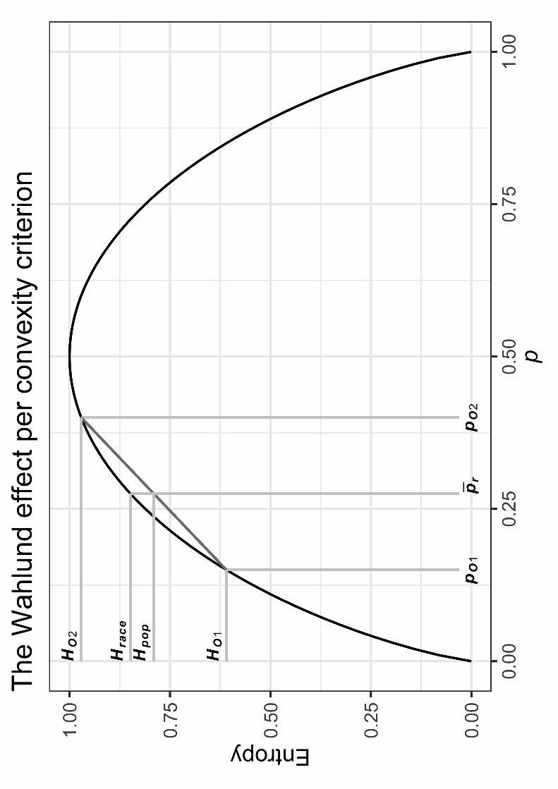
rgw1
Text Box
Fig. 1.3
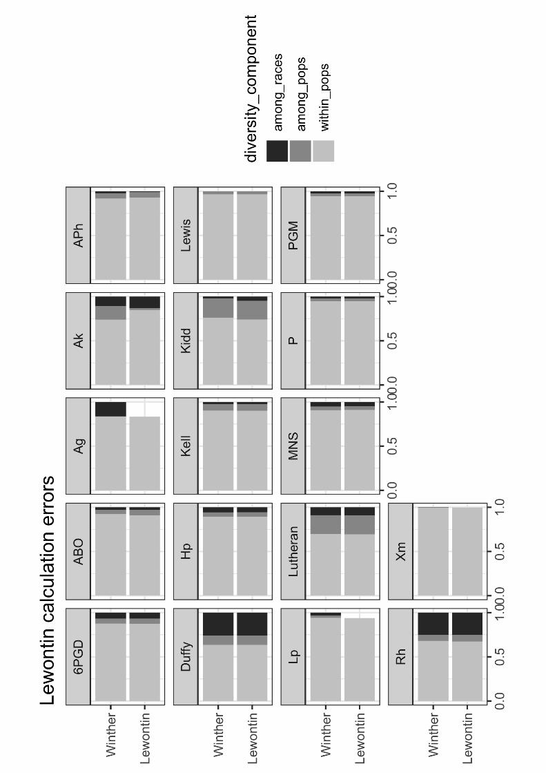
rgw1
Text Box
Fig. 1.4
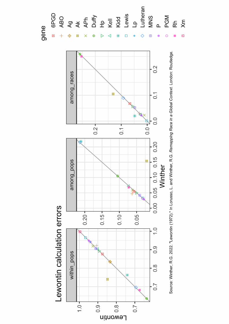
rgw1
Text Box
Fig. 1.5
Related Documents