Lecture1 Image Video Compression

April 18, 2002 Page 1John G. Apostolopoulos

Image & VideoCoding

Image and Video Compression

MIT 6.344, Spring 2002

John G. ApostolopoulosStreaming Media Systems Group

Hewlett-Packard [email protected]

John G. ApostolopoulosPage 2

Image & VideoCoding

April 18, 2002

Overview of Next Five Lectures

• Image and Video Compression (Thurs, 4/18)– Principles and practice of image/video coding

• Video Compression (Tues, 4/23)– Current video compression standards – Object-based video coding (MPEG-4)

• Compressed-Domain Video Processing (Thurs, 4/25)– Efficient processing of compressed video

• Video Communication and Video Streaming I (Tues, 4/30)– Video streaming over the Internet

• Video Communication and Video Streaming II (Thurs, 5/2)– Video communication over lossy packet networks and

wireless links → Error-resilient video communication

Today


Image & VideoCoding

April 18, 2002

Outline of Today’s Lecture

• Motivation for compression• Brief review of generic compression system (from last lecture)

– Today: Examine use of transforms for representing a signal• Image compression

– Transform, uniform quantization, Huffman coding• Video compression

– Exploit temporal dimension of video signal– Motion-compensated prediction– Generic (MPEG-type) video coder architecture


Image & VideoCoding

April 18, 2002

Motivation for Compression:Example of HDTV Video Signal

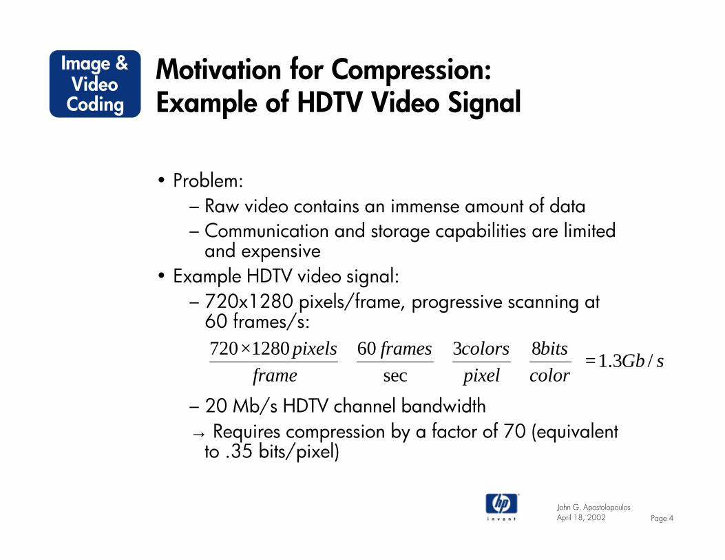
• Problem:– Raw video contains an immense amount of data– Communication and storage capabilities are limited

and expensive• Example HDTV video signal:

– 720x1280 pixels/frame, progressive scanning at 60 frames/s:

– 20 Mb/s HDTV channel bandwidth→ Requires compression by a factor of 70 (equivalent

to .35 bits/pixel)

sGbcolor

bitspixelcolorsframes

framepixels

/3.183

sec601280720

=

×


Image & VideoCoding

April 18, 2002

Achieving Compression

• Reduce redundancy and irrelevancy• Sources of redundancy

– Temporal: Adjacent frames highly correlated– Spatial: Nearby pixels are often correlated with

each other– Color space: RGB components are correlated

among themselves→ Relatively straightforward to exploit

• Irrelevancy– Perceptually unimportant information→ Difficult to model and exploit


Image & VideoCoding

April 18, 2002

Spatial and Temporal Redundancy

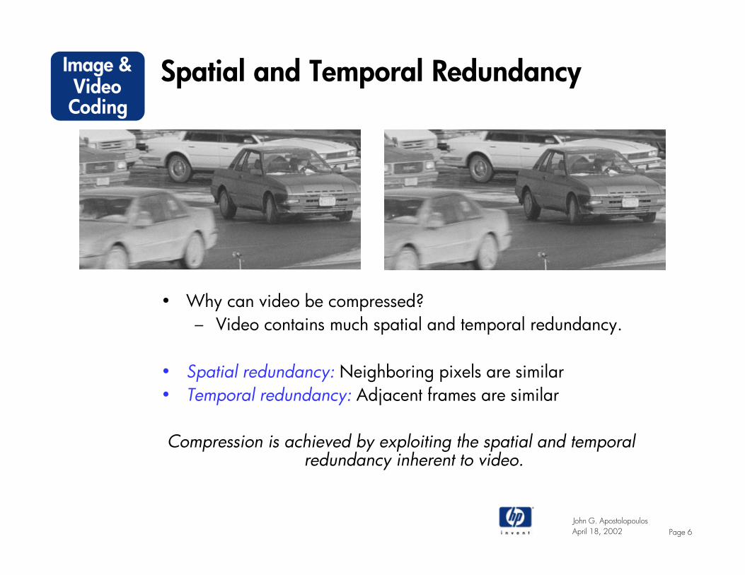
• Why can video be compressed?– Video contains much spatial and temporal redundancy.

• Spatial redundancy: Neighboring pixels are similar• Temporal redundancy: Adjacent frames are similar

Compression is achieved by exploiting the spatial and temporal redundancy inherent to video.


Image & VideoCoding

April 18, 2002







Image & VideoCoding

April 18, 2002

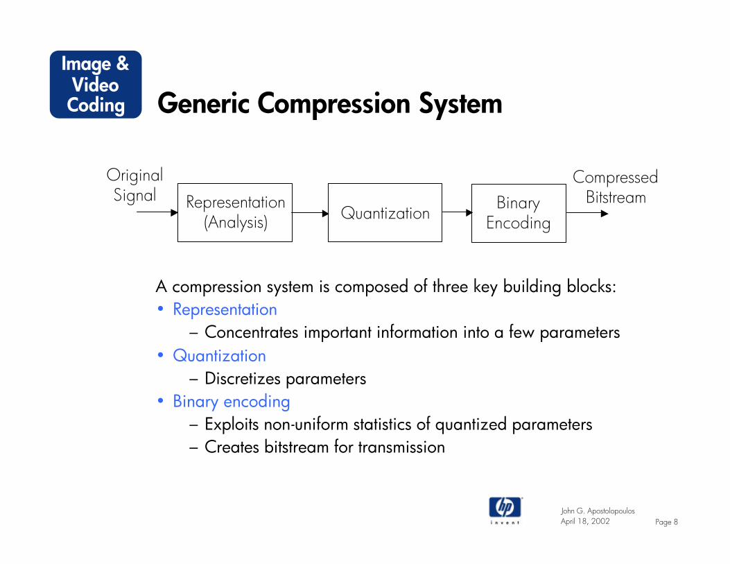
Generic Compression System

A compression system is composed of three key building blocks:• Representation

– Concentrates important information into a few parameters• Quantization

– Discretizes parameters• Binary encoding

– Exploits non-uniform statistics of quantized parameters– Creates bitstream for transmission

Representation(Analysis) Quantization Binary

Encoding

CompressedBitstream

OriginalSignal


Image & VideoCoding

April 18, 2002

Generic Compression System (cont.)

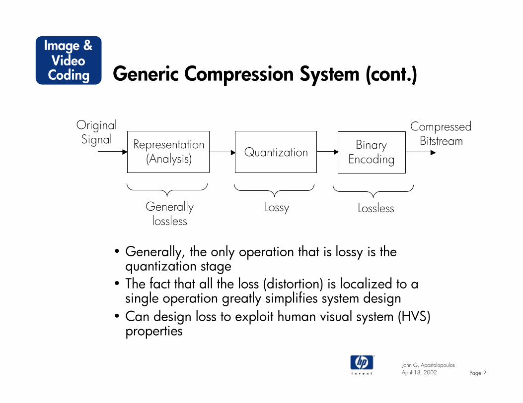
• Generally, the only operation that is lossy is the quantization stage

• The fact that all the loss (distortion) is localized to a single operation greatly simplifies system design

• Can design loss to exploit human visual system (HVS) properties

Representation(Analysis) Quantization

CompressedBitstream

OriginalSignal

Generallylossless

Lossy Lossless

BinaryEncoding


Image & VideoCoding

April 18, 2002

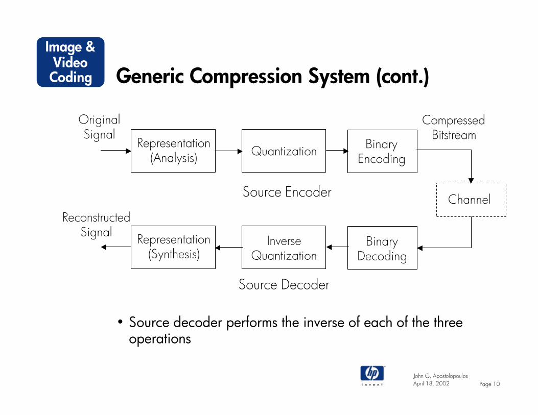
Generic Compression System (cont.)

• Source decoder performs the inverse of each of the three operations

Representation(Analysis) Quantization

CompressedBitstream

OriginalSignal

Representation(Synthesis)

InverseQuantization

ChannelReconstructed

Signal

Source Encoder

Source Decoder

BinaryEncoding

BinaryDecoding


Image & VideoCoding

April 18, 2002







Image & VideoCoding

April 18, 2002

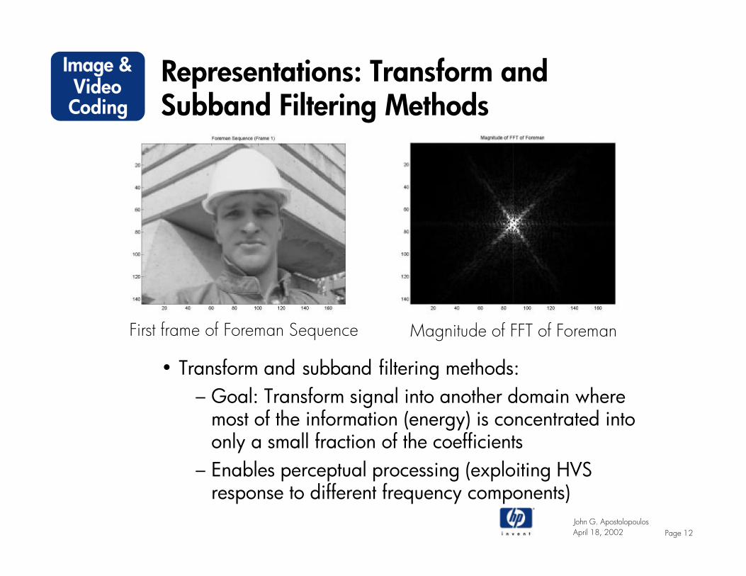
Representations: Transform and Subband Filtering Methods

• Transform and subband filtering methods:– Goal: Transform signal into another domain where

most of the information (energy) is concentrated into only a small fraction of the coefficients

– Enables perceptual processing (exploiting HVS response to different frequency components)

First frame of Foreman Sequence Magnitude of FFT of Foreman


Image & VideoCoding

April 18, 2002

Transform Image Coding

• A good transform provides:– Most of the image energy is concentrated into a

small fraction of the coefficients– Coding only these small fraction of the coefficients

and discarding the rest can often lead to excellent reconstructed quality

→ The more energy compaction the better!• Orthogonal transforms are particularly useful

– Energy in discarded coefficients is equal to energy in reconstruction error


Image & VideoCoding

April 18, 2002

Possible Transforms for Image Coding

• Karhunen-Loeve Transform (KLT)– Optimal energy compaction– Requires knowledge of signal covariance– In general, no simple computational algorithm

• Discrete Fourier Transform (DFT)– Fast algorithms– Good energy compaction, but not as good as DCT

• Discrete Cosine Transform (DCT)– Fast algorithms– Good energy compaction– All real coefficients– Overall good performance and widely used for image

and video coding


Image & VideoCoding

April 18, 2002

Global DCT versus Block DCT

• Basic question: Compute DCT over the entire image (global DCT) or over each small part?

• Observation: Image content varies significantly across different parts of the image, difficult to exploit with a global transform

• Block-DCT– Partition image into 8x8 pixel blocks– Compute 2-D DCT of each block

• Advantages of Block-DCT– Reduced computation– Suitable for parallel processing– Enables adaptive encoding: Can easily allocate

more bits to blocks that are more important


Image & VideoCoding

April 18, 2002

Discrete Cosine Transform (DCT)

• 1-D Discrete Cosine Transform (N-point):

• 1-D DCT basis vectors:

• 2-D DCT: Separable transform of 1-D DCT• 2-D DCT basis vectors?

– Basis pictures!

( ) ( )

−=

==

+

= ∑−

=

1,...,2,12

01)(

where2

12cos)()(

1

0

NkN

kNk

Nkn

nskkCN

n

α

πα

( ) ( )

+

=N

knknbk 2

12cos)(

πα


Image & VideoCoding

April 18, 2002

2-D Discrete Cosine Transform

• 2-D basis vectors for 2-D DCT are basis pictures!• 64 basis pictures for 8x8-pixel 2-D DCT• Image coding with the 2-D DCT is equivalent to approximating

the image as a linear combination of these basis pictures!


Image & VideoCoding

April 18, 2002

Coding Transform Coefficients

Selecting the basis pictures to approximate an image is equivalent to selecting the DCT coefficients to code

General methods of coding/discarding coefficients:1. Zonal coding:

– Code all coefficients in a zone and discard others– Example zone: Spatial low frequencies– Only need to code coefficient amplitudes

2. Threshold coding:– Keep coefficients with magnitude above a threshold– Coefficient amplitudes and locations must be coded– Provides best performance

k1

k2

Discard

Code


Image & VideoCoding

April 18, 2002

Comments on Transform and Subband Filtering Methods

• Examples of “traditional” transforms:– KLT, DFT, DCT

• Examples of “traditional” subband filtering methods:– Perfect reconstruction filterbanks, wavelets

• Transform and subband interpretations:– All of the above are linear representations and can be interpreted

from either a transform or a subband filtering viewpoint• Transform viewpoint:

– Express signal as a linear combination of basis vectors– Stresses linear expansion (linear algebra) perspective

• Subband filtering viewpoint:– Pass signal through a set of filters and examine the frequencies

passed by each filter (subband)– Stresses filtering (signal processing) perspective


Image & VideoCoding

April 18, 2002

Transform/Subband Representations:Wavelet Transform• Wavelet transform provides basis vectors at different scales:

– High frequency basis vectors with small support– Good for “edges”

– Low frequency basis vectors with large support– Good for slowly varying lowpass components

• Highly simplifed → I’ll be happy to talk about these in detail…

Example: 3-level 2-D WT,10 2-D basis pictures

Both transform and subband filtering viewpoints provide important insights

into designing and using wavelets


Image & VideoCoding

April 18, 2002







Image & VideoCoding

April 18, 2002

Image Compression

• Goal: High quality image approximation using a small number of bits

• Must reduce redundancy and irrelevancy• Examine representation along:

– Spatial dimension– Color space dimension

• Quantization• Binary encoding


Image & VideoCoding

April 18, 2002

Spatial Processing:Transform/Subband Methods

• Transform/subband methods– KLT, DFT, DCT– Subband filtering, LOT, wavelets

• Desired properties– High energy compaction– Fast computation (separable, and fast algorithms)

• Discrete Cosine Transform (DCT)– Good energy compaction (better than DFT)– Fast algorithms exist– Block DCT


Image & VideoCoding

April 18, 2002

Spatial Processing:Block DCT

• Block DCT– Partition image into 8x8 pixel blocks– Each block independently transformed and processed

– Compute 8x8 2-D DCT of each block– Quantize and encode each block

• Advantages:– Enables simple, spatially-adaptive processing– Reduces computation and memory requirements– Suitable for parallel processing

• Basic building block for most current image and video compression standards including:

– JPEG, MPEG-1/2/4, H.261/3/L


Image & VideoCoding

April 18, 2002

Spatial Processing:Wavelet Transform

• Wavelet transform:– Provides good energy compaction– Better match to “edges” than Block DCT

• Overall, provides better compression performance than Block DCT for still image coding

– Basic building block for JPEG-2000• Has not gained acceptance in video coding standards

– Not a good match for block-matching ME (discussed later in this lecture)

– Also significant inertia behind Block DCT


Image & VideoCoding

April 18, 2002

Color Space Processing

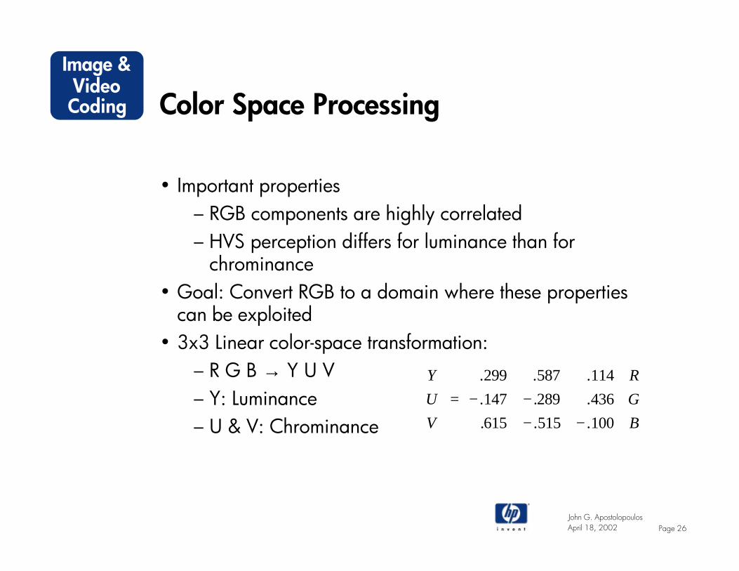
• Important properties– RGB components are highly correlated– HVS perception differs for luminance than for

chrominance• Goal: Convert RGB to a domain where these properties

can be exploited• 3x3 Linear color-space transformation:

– R G B → Y U V– Y: Luminance– U & V: Chrominance

−−−−=

BGR

VUY

100.515.615.436.289.147.114.587.299.


Image & VideoCoding

April 18, 2002

Color Space Processing (cont.)

Advantages of color space conversion:• HVS has lower spatial frequency response to U and V

than to Y→ Reduce sampling density for U and V

• HVS has lower sensitivity to U and V than to Y→ Quantize U and V more coarsely

• Comment:– While an RGB signal would appear to require 3

times the number of bits of a single-color image, it only requires <1.5 times as many bits


Image & VideoCoding

April 18, 2002

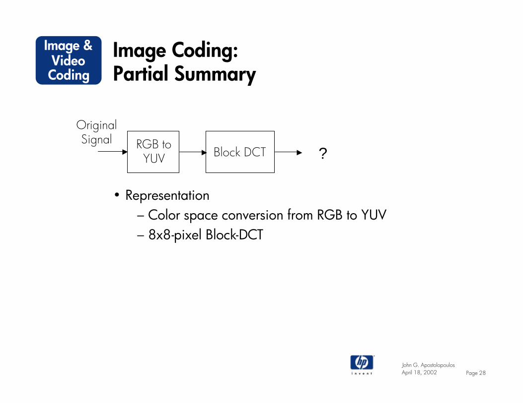
Image Coding:Partial Summary

• Representation– Color space conversion from RGB to YUV– 8x8-pixel Block-DCT

RGB toYUV Block DCT

OriginalSignal

?


Image & VideoCoding

April 18, 2002

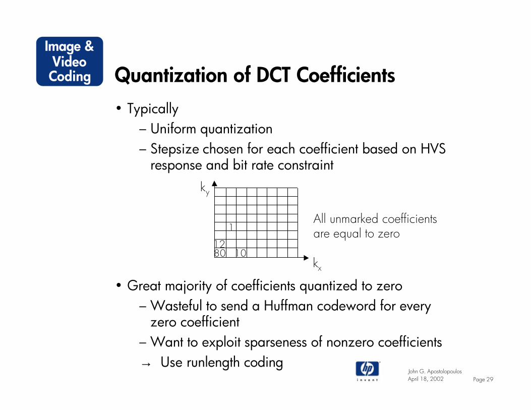
Quantization of DCT Coefficients• Typically

– Uniform quantization– Stepsize chosen for each coefficient based on HVS

response and bit rate constraint

• Great majority of coefficients quantized to zero– Wasteful to send a Huffman codeword for every

zero coefficient– Want to exploit sparseness of nonzero coefficients→ Use runlength coding

ky

kx

8012

10

1All unmarked coefficientsare equal to zero


Image & VideoCoding

April 18, 2002

Runlength Coding and Zigzag Scanning of DCT Coefficients

• Runlength coding: – Encode each run of consecutive zeros between

nonzero quantized coefficients– Length of consecutive zeros: runlength

• Order coefficients by zigzag scanning:– Exploit the fact that most of the non-zero coefficients

are in the low frequencies– Increase the runlengths of zero-valued coefficients– Basically cluster non-zero coefficients at the

beginning and zero coefficients at the end• End of block (EOB) marker to signify that all subsequent

coefficients are zero


Image & VideoCoding

April 18, 2002

Example: Runlength Coding and Zigzag Scanning of DCT Coefficients

• Zigzag scanned DCT coefficients: 80, 0, 12, 0, 0, 10, 0, 0, 0, 0, 0, 1, 0, 0, 0, 0, …, 0

• Coding symbols:80, (1,12), (2,10), (5,1), EOB

• Notes:– DC coefficient is always non-zero for an image and always coded– (n,m) is (run,value) pair

ky

kx

ky

kx

8012

10

1


Image & VideoCoding

April 18, 2002

Image Compression: Summary

• Coding an image (single frame):– RGB to YUV color-space conversion– Partition image into 8x8-pixel blocks– 2-D DCT of each block– Quantize each DCT coefficient– Runlength and Huffman code the nonzero quantized DCT

coefficients→ Basis for the JPEG Image Compression Standard→ JPEG-2000 uses wavelet transform and arithmetic coding

Quantization

CompressedBitstream

OriginalImage Runlength &

HuffmanCoding

RGBto

YUVBlock DCT


Image & VideoCoding

April 18, 2002







Image & VideoCoding

April 18, 2002

Video Compression

• Video: Sequence of frames (images) that are related• Related along the temporal dimension

– Therefore temporal redundancy exists• Main addition over image compression

– Temporal redundancy→ Video coder must exploit the temporal redundancy


Image & VideoCoding

April 18, 2002

Temporal Processing

• Usually high frame rate: Significant temporal redundancy• Possible representations along temporal dimension:

– Transform/subband methods– Good for textbook case of constant velocity uniform

global motion– Inefficient for nonuniform motion, I.e. real-world motion– Requires large number of frame stores

– Leads to delay (Memory cost may also be an issue)

– Predictive methods– Good performance using only 2 frame stores– However, simple frame differencing in not enough


Image & VideoCoding

April 18, 2002

Video Compression

• Main addition over image compression: – Exploit the temporal redundancy

• Predict current frame based on previously coded frames• Three types of coded frames:

– I-frame: Intra-coded frame, coded independently of all other frames

– P-frame: Predictively coded frame, coded based on previously coded frame

– B-frame: Bi-directionally predicted frame, coded based on both previous and future coded frames

I frame P-frame B-frame


Image & VideoCoding

April 18, 2002

Temporal Processing:Motion-Compensated Prediction

• Simple frame differencing fails when there is motion• Must account for motion

→ Motion-compensated (MC) prediction• MC-prediction generally provides significant improvements• Questions:

– How can we estimate motion?– How can we form MC-prediction?


Image & VideoCoding

April 18, 2002

Temporal Processing:Motion Estimation

• Ideal situation:– Partition video into moving objects– Describe object motion→ Generally very difficult

• Practical approach: Block-Matching Motion Estimation– Partition each frame into blocks– Describe motion of each block→ No object identification required→ Good, robust performance


Image & VideoCoding

April 18, 2002

Block-Matching Motion Estimation

• Assumptions:– Translational motion within block:

– All pixels within each block have the same motion• ME Algorithm:

– Divide current frame into non-overlapping N1xN2 blocks– For each block, find the best matching block in reference frame

• MC-Prediction Algorithm:– Use best matching blocks of reference frame as prediction of

blocks in current frame

16 15 14

13

12 11

10 9

8 7 6

5

4 3 2

1

16 15

14 13

12 11

10 9

8 7

6 5

4 3

2 1

Reference Frame Current Frame

),,(),,( 221121 refcur kmvnmvnfknnf −−=

Motion Vector(mv1, mv2)


Image & VideoCoding

April 18, 2002

Block Matching:Determining the Best Matching Block

• For each block in the current frame search for best matching block in the reference frame

– Metrics for determining “best match”:

– Candidate blocks: – Strategies for searching candidate blocks for best match

– Full search: Examine all candidate blocks– Partial (fast) search: Examine a carefully selected subset

• Estimate of motion for best matching block: “motion vector”

( )[ ]( )∑ ∑

∈−−−=

21,

2221121 ),,(,,

nn Blockrefcur kmvnmvnfknnfMSE

( )( )∑ ∑

∈

−−−=21,

221121 ),,(,,nn Block

refcur kmvnmvnfknnfMAE

( ) area pixel 32,32 e.g., in, blocks All ±±


Image & VideoCoding

April 18, 2002

Motion Vectors and Motion Vector Field

• Motion vector– Expresses the relative horizontal and vertical offsets

(mv1,mv2), or motion, of a given block from one frame to another

– Each block has its own motion vector• Motion vector field

– Collection of motion vectors for all the blocks in a frame


Image & VideoCoding

April 18, 2002

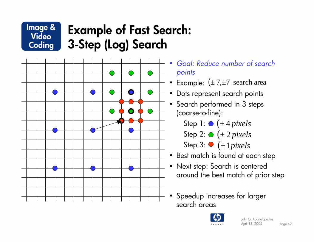
Example of Fast Search:3-Step (Log) Search

• Goal: Reduce number of search points

• Example:• Dots represent search points• Search performed in 3 steps

(coarse-to-fine):Step 1:Step 2:Step 3:

• Best match is found at each step• Next step: Search is centered

around the best match of prior step

• Speedup increases for larger search areas

( )pixels4±( )pixels2±( )pixels1±

( ) areasearch 7,7 ±±


Image & VideoCoding

April 18, 2002

Motion Vector Precision?

• Motivation:– Motion is not limited to integer-pixel offsets– However, video only known at discrete pixel locations– To estimate sub-pixel motion, frames must be spatially

interpolated• Fractional MVs are used to represent the sub-pixel motion• Improved performance (extra complexity is worthwhile)• Half-pixel ME used in most standards: MPEG-1/2/4• Why are half-pixel motion vectors better?

– Can capture half-pixel motion– Averaging effect (from spatial interpolation) reduces

prediction error → Improved prediction– For noisy sequences, averaging effect reduces noise →

Improved compression


Image & VideoCoding

April 18, 2002

Practical Half-Pixel Motion Estimation Algorithm

• Half-pixel ME (coarse-fine) algorithm:1) Coarse step: Perform integer motion estimation on blocks; find

best integer-pixel MV2) Fine step: Refine estimate to find best half-pixel MV

a) Spatially interpolate the selected region in reference frameb) Compare current block to interpolated reference frame

blockc) Choose the integer or half-pixel offset that provides best

match• Typically, bilinear interpolation is used for spatial interpolation


Image & VideoCoding

April 18, 2002

Example: MC-Prediction for Two Consecutive Frames

Previous Frame(Reference Frame)

Current Frame(To be Predicted)

16 15 14 13

12 11 10 9

8 7 6

5

4 3 2 1

16 15 14

13

12 11 10 9

8 7

6 5

4 3 2 1

Reference Frame Predicted Frame


Image & VideoCoding

April 18, 2002

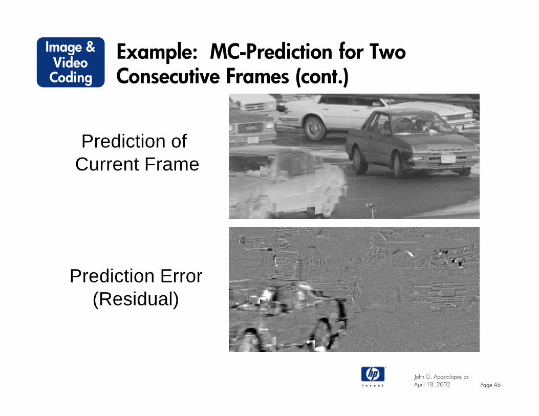
Example: MC-Prediction for Two Consecutive Frames (cont.)

Prediction of Current Frame

Prediction Error(Residual)


Image & VideoCoding

April 18, 2002

Block Matching Algorithm: Summary• Issues:

– Block size?– Search range?– Motion vector accuracy?

• Motion typically estimated only from luminance• Advantages:

– Good, robust performance for compression– Resulting motion vector field is easy to represent (one MV

per block) and useful for compression– Simple, periodic structure, easy VLSI implementations

• Disadvantages:– Assumes translational motion model → Breaks down for

more complex motion– Often produces blocking artifacts (OK for coding with

Block DCT)


Image & VideoCoding

April 18, 2002

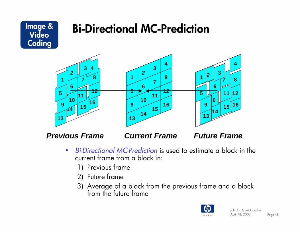
Bi-Directional MC-Prediction

• Bi-Directional MC-Prediction is used to estimate a block in the current frame from a block in:1) Previous frame2) Future frame3) Average of a block from the previous frame and a block

from the future frame

161514

13

1211

109

876

5

432

1

1615

1413

1211

109

87

65

43

21

Previous Frame Current Frame

161514

13

121110

9

876

5

4

321

Future Frame


Image & VideoCoding

April 18, 2002

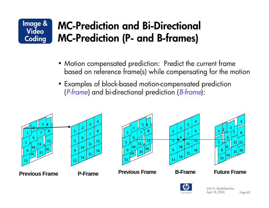
MC-Prediction and Bi-Directional MC-Prediction (P- and B-frames)

• Motion compensated prediction: Predict the current frame based on reference frame(s) while compensating for the motion

• Examples of block-based motion-compensated prediction (P-frame) and bi-directional prediction (B-frame):

161514

13

1211

109

876

5

432

1

1615

1413

1211

109

87

65

43

21

Previous Frame B-Frame

161514

13

121110

9

876

5

4

321

Future Frame

161514

13

1211

109

876

5

432

1

1615

1413

1211

109

87

65

43

21

Previous Frame P-Frame


Image & VideoCoding

April 18, 2002

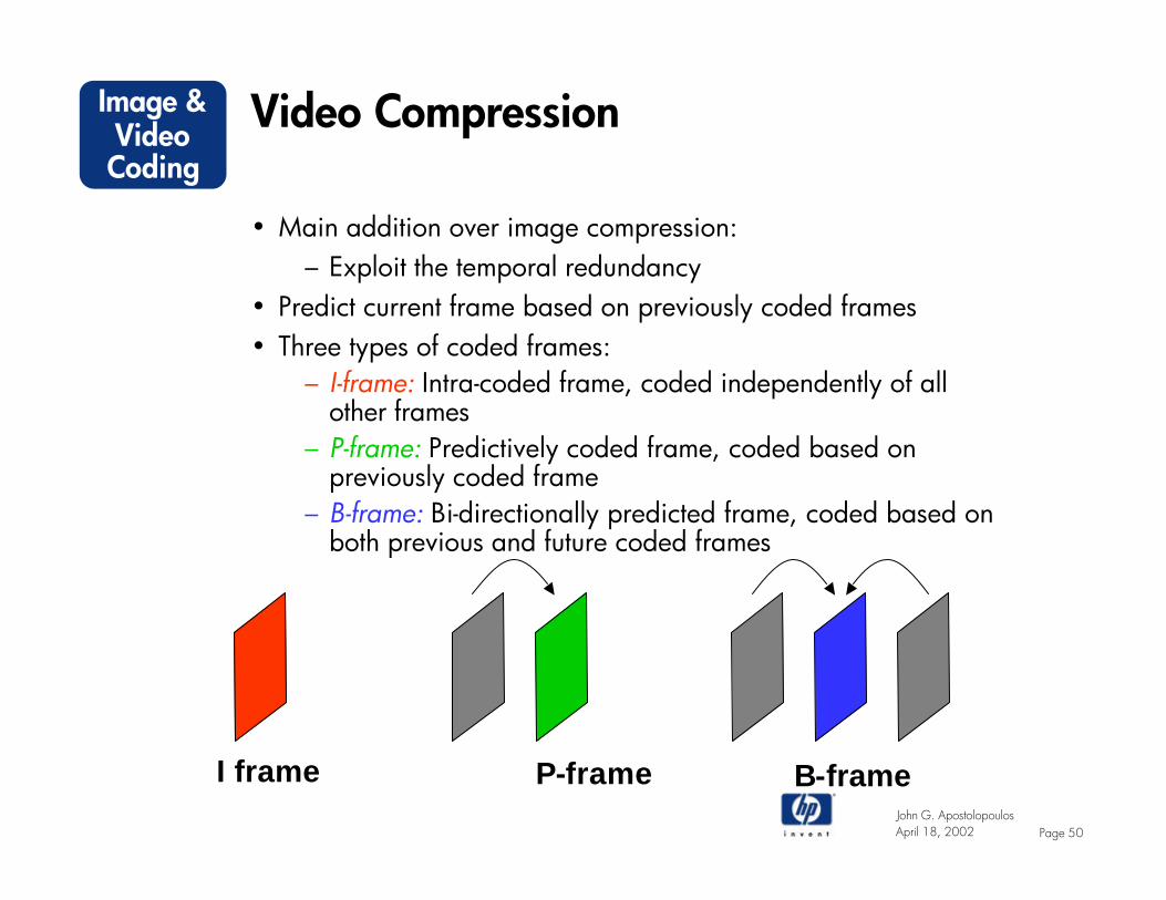
Video Compression

• Main addition over image compression: – Exploit the temporal redundancy

• Predict current frame based on previously coded frames• Three types of coded frames:

– I-frame: Intra-coded frame, coded independently of all other frames

– P-frame: Predictively coded frame, coded based on previously coded frame

– B-frame: Bi-directionally predicted frame, coded based on both previous and future coded frames

I frame P-frame B-frame


Image & VideoCoding

April 18, 2002

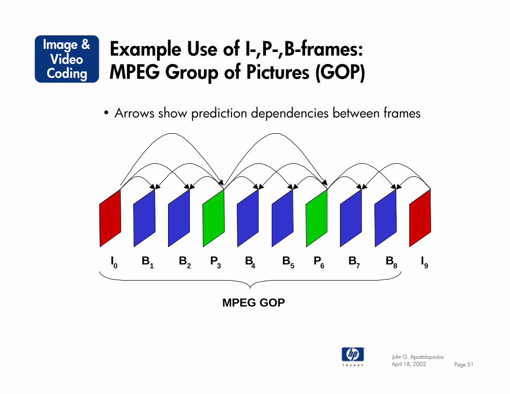
Example Use of I-,P-,B-frames: MPEG Group of Pictures (GOP)

• Arrows show prediction dependencies between frames

MPEG GOP

I0 B1 B2 P3 B4 B5 P6 B7 B8 I9


Image & VideoCoding

April 18, 2002

Summary of Temporal Processing

• Use MC-prediction (P and B frames) to reduce temporal redundancy

• MC-prediction usually performs well; In compression have a second chance to recover when it performs badly

• MC-prediction yields:– Motion vectors– MC-prediction error or residual → Code error with

conventional image coder• Sometimes MC-prediction may perform badly

– Examples: Complex motion, new imagery (occlusions)– Approach:

1. Identify blocks where prediction fails 2. Code block without prediction


Image & VideoCoding

April 18, 2002

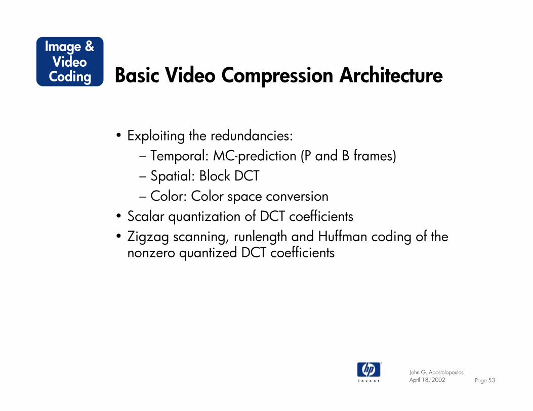
Basic Video Compression Architecture

• Exploiting the redundancies:– Temporal: MC-prediction (P and B frames)– Spatial: Block DCT– Color: Color space conversion

• Scalar quantization of DCT coefficients• Zigzag scanning, runlength and Huffman coding of the

nonzero quantized DCT coefficients


Image & VideoCoding

April 18, 2002

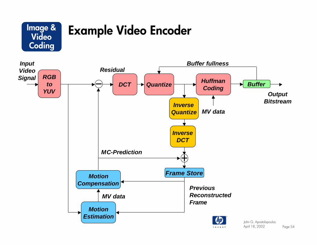
Example Video Encoder

DCT HuffmanCoding

MotionEstimation

MotionCompensation

BufferRGB

toYUV

MV data

MV data

MC-Prediction

ResidualInputVideoSignal

OutputBitstream

Quantize

InverseDCT

InverseQuantize

PreviousReconstructedFrame

Buffer fullness

Frame Store


Image & VideoCoding

April 18, 2002

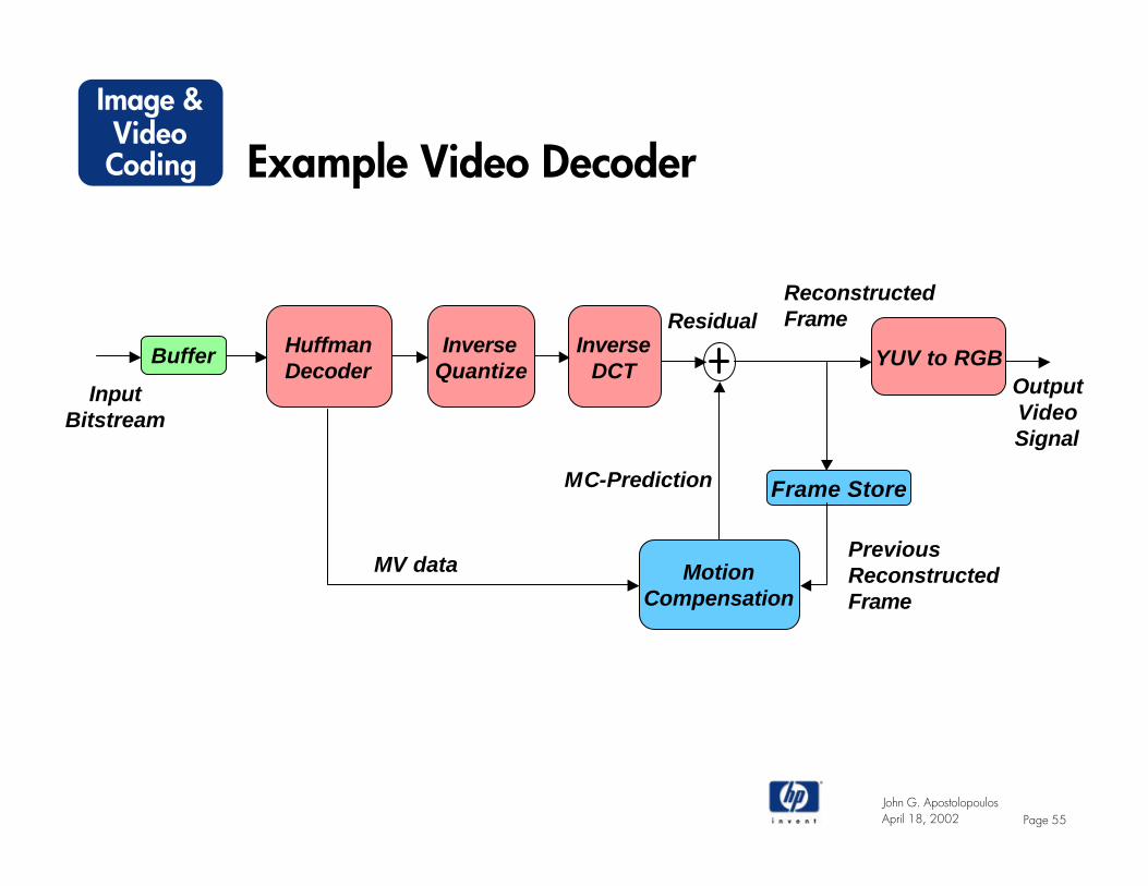
Example Video Decoder

HuffmanDecoder

MotionCompensation

Buffer YUV to RGB

MV data

ReconstructedFrame

OutputVideoSignal

InputBitstream

MC-Prediction

ResidualInverse

DCTInverse

Quantize

Frame Store

PreviousReconstructedFrame


Image & VideoCoding

April 18, 2002

Review of Today’s Lecture






Image & VideoCoding

April 18, 2002

Next Lecture

• Continue video compression– Generic (MPEG-type) video coder architecture– Scalable video coding

• Current video compression standards– What do the standards specify?– Frame-based video coding: MPEG-1/2/4, H.261/3– Object-based video coding: MPEG-4

• Object-based video coding (MPEG-4)

Lecture1 Image Video Compression

Documents