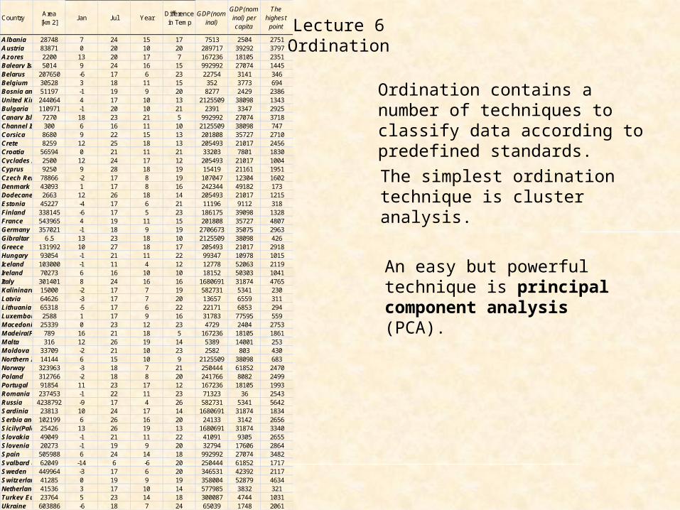
Lecture 6 Ordination C ountry Area [km 2] Jan Jul Y ear Difference in Tem p GDP(nom inal) GDP(nom inal) per capita T he highes t point A lbania 28748 7 24 15 17 7513 2504 2751 A ustria 83871 0 20 10 20 289717 39292 3797 Azores 2200 13 20 17 7 167236 18105 2351 Baleary Isl 5014 9 24 16 15 992992 27074 1445 Belarus 207650 -6 17 6 23 22754 3141 346 Belgium 30528 3 18 11 15 352 3773 694 Bosnia an 51197 -1 19 9 20 8277 2429 2386 United Kin 244064 4 17 10 13 2125509 38098 1343 Bulgaria 110971 -1 20 10 21 2391 3347 2925 C anary Isla 7270 18 23 21 5 992992 27074 3718 Channel Is 300 6 16 11 10 2125509 38098 747 Corsica 8680 9 22 15 13 201808 35727 2710 C rete 8259 12 25 18 13 205493 21017 2456 C roatia 56594 0 21 11 21 33203 7801 1830 Cyclades I 2500 12 24 17 12 205493 21017 1004 Cyprus 9250 9 28 18 19 15419 21161 1951 Czech Rep 78866 -2 17 8 19 107047 12304 1602 Denmark 43093 1 17 8 16 242344 49182 173 Dodecane 2663 12 26 18 14 205493 21017 1215 E stonia 45227 -4 17 6 21 11196 9112 318 Finland 338145 -6 17 5 23 186175 39098 1328 France 543965 4 19 11 15 201808 35727 4807 Germany 357021 -1 18 9 19 2706673 35075 2963 G ibraltar 6.5 13 23 18 10 2125509 38098 426 Greece 131992 10 27 18 17 205493 21017 2918 Hungary 93054 -1 21 11 22 99347 10978 1015 Iceland 103000 -1 11 4 12 12778 52063 2119 Ireland 70273 6 16 10 10 18152 50303 1041 Italy 301401 8 24 16 16 1680691 31874 4765 Kaliningra 15000 -2 17 7 19 582731 5341 230 L atvia 64626 -3 17 7 20 13657 6559 311 Lithuania 65318 -5 17 6 22 22171 6853 294 Luxembou 2588 1 17 9 16 31783 77595 559 Macedoni 25339 0 23 12 23 4729 2404 2753 Madeira(F 789 16 21 18 5 167236 18105 1861 Malta 316 12 26 19 14 5389 14001 253 Moldova 33709 -2 21 10 23 2582 803 430 Northern I 14144 6 15 10 9 2125509 38098 683 Norway 323963 -3 18 7 21 250444 61852 2470 Poland 312766 -2 18 8 20 241766 8082 2499 Portugal 91854 11 23 17 12 167236 18105 1993 Romania 237453 -1 22 11 23 71323 36 2543 Russia 4238792 -9 17 4 26 582731 5341 5642 S ardinia 23813 10 24 17 14 1680691 31874 1834 S erbia and 102199 6 26 16 20 24133 3142 2656 S icily(Pale 25426 13 26 19 13 1680691 31874 3340 S lovakia 49049 -1 21 11 22 41091 9305 2655 S lovenia 20273 -1 19 9 20 32794 17606 2864 S pain 505988 6 24 14 18 992992 27074 3482 S valbard & 62049 -14 6 -6 20 250444 61852 1717 S weden 449964 -3 17 6 20 346531 42392 2117 S witz erlan 41285 0 19 9 19 358004 52879 4634 Netherland 41536 3 17 10 14 577985 3832 321 Turkey Eu 23764 5 23 14 18 300087 4744 1031 Ukraine 603886 -6 18 7 24 65039 1748 2061 Ordination contains a number of techniques to classify data according to predefined standards. The simplest ordination technique is cluster analysis. An easy but powerful technique is principal component analysis (PCA).

Lecture 6 Ordination Ordination contains a number of techniques to classify data according to predefined standards. The simplest ordination technique is.
Dec 19, 2015
Welcome message from author
This document is posted to help you gain knowledge. Please leave a comment to let me know what you think about it! Share it to your friends and learn new things together.
Transcript
Lecture 6Ordination
CountryArea [km2]
Jan Jul YearDifference in Temp
GDP(nominal)
GDP(nominal) per capita
The highest point
Albania 28748 7 24 15 17 7513 2504 2751Austria 83871 0 20 10 20 289717 39292 3797Azores 2200 13 20 17 7 167236 18105 2351Baleary Islands5014 9 24 16 15 992992 27074 1445Belarus 207650 -6 17 6 23 22754 3141 346Belgium 30528 3 18 11 15 352 3773 694Bosnia and Herzegovina51197 -1 19 9 20 8277 2429 2386United Kingdom244064 4 17 10 13 2125509 38098 1343Bulgaria 110971 -1 20 10 21 2391 3347 2925Canary Islands7270 18 23 21 5 992992 27074 3718Channel Is. 300 6 16 11 10 2125509 38098 747Corsica 8680 9 22 15 13 201808 35727 2710Crete 8259 12 25 18 13 205493 21017 2456Croatia 56594 0 21 11 21 33203 7801 1830Cyclades Is. 2500 12 24 17 12 205493 21017 1004Cyprus 9250 9 28 18 19 15419 21161 1951Czech Republic78866 -2 17 8 19 107047 12304 1602Denmark 43093 1 17 8 16 242344 49182 173Dodecanese Is.2663 12 26 18 14 205493 21017 1215Estonia 45227 -4 17 6 21 11196 9112 318Finland 338145 -6 17 5 23 186175 39098 1328France 543965 4 19 11 15 201808 35727 4807Germany 357021 -1 18 9 19 2706673 35075 2963Gibraltar 6.5 13 23 18 10 2125509 38098 426Greece 131992 10 27 18 17 205493 21017 2918Hungary 93054 -1 21 11 22 99347 10978 1015Iceland 103000 -1 11 4 12 12778 52063 2119Ireland 70273 6 16 10 10 18152 50303 1041Italy 301401 8 24 16 16 1680691 31874 4765Kaliningrad Region15000 -2 17 7 19 582731 5341 230Latvia 64626 -3 17 7 20 13657 6559 311Lithuania 65318 -5 17 6 22 22171 6853 294Luxembourg2588 1 17 9 16 31783 77595 559Macedonia 25339 0 23 12 23 4729 2404 2753Madeira(Funchal)789 16 21 18 5 167236 18105 1861Malta 316 12 26 19 14 5389 14001 253Moldova 33709 -2 21 10 23 2582 803 430Northern Ireland14144 6 15 10 9 2125509 38098 683Norway 323963 -3 18 7 21 250444 61852 2470Poland 312766 -2 18 8 20 241766 8082 2499Portugal 91854 11 23 17 12 167236 18105 1993Romania 237453 -1 22 11 23 71323 36 2543Russia 4238792 -9 17 4 26 582731 5341 5642Sardinia 23813 10 24 17 14 1680691 31874 1834Serbia and Montenegro102199 6 26 16 20 24133 3142 2656Sicily(Palermo)25426 13 26 19 13 1680691 31874 3340Slovakia 49049 -1 21 11 22 41091 9305 2655Slovenia 20273 -1 19 9 20 32794 17606 2864Spain 505988 6 24 14 18 992992 27074 3482Svalbard & Jan Mayen62049 -14 6 -6 20 250444 61852 1717Sweden 449964 -3 17 6 20 346531 42392 2117Switzerland 41285 0 19 9 19 358004 52879 4634Netherlands 41536 3 17 10 14 577985 3832 321Turkey European part23764 5 23 14 18 300087 4744 1031Ukraine 603886 -6 18 7 24 65039 1748 2061
Ordination contains a number of techniques to classify data according to predefined standards.
The simplest ordination technique is cluster analysis.
An easy but powerful technique is principal component analysis (PCA).
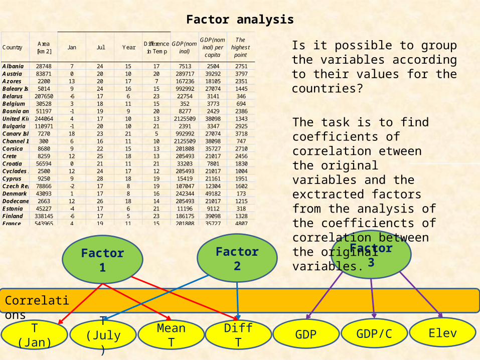
Factor analysis
CountryArea [km2]
Jan Jul YearDifference in Temp
GDP(nominal)
GDP(nominal) per capita
The highest point
Albania 28748 7 24 15 17 7513 2504 2751Austria 83871 0 20 10 20 289717 39292 3797Azores 2200 13 20 17 7 167236 18105 2351Baleary Islands5014 9 24 16 15 992992 27074 1445Belarus 207650 -6 17 6 23 22754 3141 346Belgium 30528 3 18 11 15 352 3773 694Bosnia and Herzegovina51197 -1 19 9 20 8277 2429 2386United Kingdom244064 4 17 10 13 2125509 38098 1343Bulgaria 110971 -1 20 10 21 2391 3347 2925Canary Islands7270 18 23 21 5 992992 27074 3718Channel Is. 300 6 16 11 10 2125509 38098 747Corsica 8680 9 22 15 13 201808 35727 2710Crete 8259 12 25 18 13 205493 21017 2456Croatia 56594 0 21 11 21 33203 7801 1830Cyclades Is. 2500 12 24 17 12 205493 21017 1004Cyprus 9250 9 28 18 19 15419 21161 1951Czech Republic78866 -2 17 8 19 107047 12304 1602Denmark 43093 1 17 8 16 242344 49182 173Dodecanese Is.2663 12 26 18 14 205493 21017 1215Estonia 45227 -4 17 6 21 11196 9112 318Finland 338145 -6 17 5 23 186175 39098 1328France 543965 4 19 11 15 201808 35727 4807Germany 357021Gibraltar 6.5Greece 131992Hungary 93054Iceland 103000Ireland 70273Italy 301401
15000Latvia 64626Lithuania 65318
258825339789
Malta 316Moldova 33709
14144Norway 323963Poland 312766Portugal 91854Romania 237453Russia 4238792Sardinia 23813
10219925426
Slovakia 49049Slovenia 20273Spain 505988
62049Sweden 449964
4128541536
Ukraine 603886
Is it possible to group the variables according to their values for the countries?
T (Jan) T (July) Mean T Diff T GDP GDP/C Elev
Factor 1 Factor 2 Factor 3
Correlations
The task is to find coefficients of correlation etween the original variables and the exctracted factors from the analysis of the coefficiencts of correlation between the original variables.
A
1
2
3
4
5
6
1
2
3
4
5
6
B C D E
z1a
z2a
z3a
z4a
z5a
z6a
z1b
z2b
z3b
z4b
z5b
z6b
z1c
z2c
z3c
z4c
z5c
z6c
z1d
z2d
z3d
z4d
z5d
z6d
z1e
z2e
z3e
z4e
z5e
z6e
F1 F2
f11
f21
f31
f41
f51
f61
f12
f22
f32
f42
f52
f62
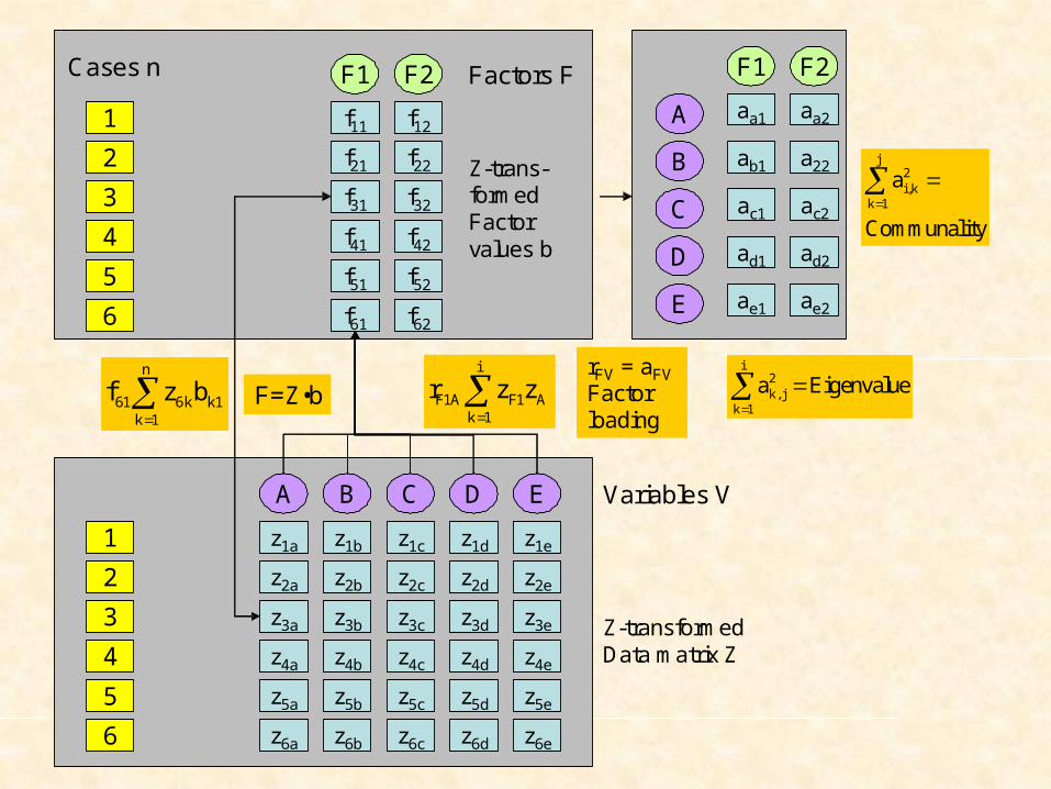
Z-transformedData matrix Z
Z-trans-formedFactorvalues b
Cases n
Variables V
Factors F
rFV = aFVFactorloading
j2i,k
k 1
a
Communality
F1 F2
A
B
C
D
E
aa1
ab1
ac1
ad1
ae1
aa2
a22
ac2
ad2
ae2
i2k , j
k 1
a Eigenvalue
F=Z•bn
61 6k k1k 1
f z b
i
F1A F1 Ak 1
r z z
n
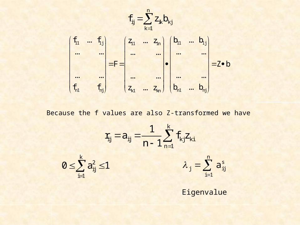
ij ik kjk 1
f z b
11 1j 11 1j11 1n
n1 nj n1 njk1 kn
f ... f b ... bz ... z
... ... ... ...... ...
F Z b
... ... ... ...... ...
f f b ... bz ... z
k
ij ij kj kin 1
1r a f z
n 1
Because the f values are also Z-transformed we have
k2ij
i 1
0 a 1
n
sj ij
i 1
a
Eigenvalue
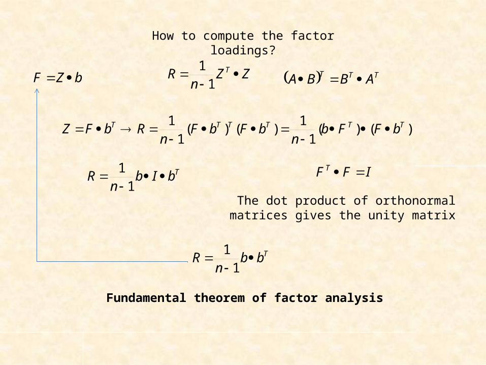
How to compute the factor loadings?
The dot product of orthonormal matrices gives the unity matrix
Fundamental theorem of factor analysis
)()(1
1)()(
11 TTTTTT bFFb
nbFbF
nRbFZ
ZZn
R T
1
1 TTT ABBA
IFF T TbIbn
R
1
1
Tbbn
R
1
1
bZF
1
2
3
4
5
6
F1 F2
f11
f21
f31
f41
f51
f61
f12
f22
f32
f42
f52
f62
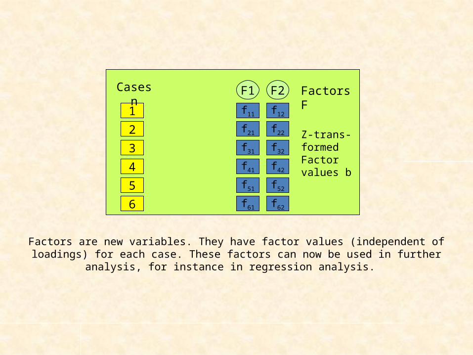
Z-trans-formed Factor values b
Cases n Factors F
Factors are new variables. They have factor values (independent of loadings) for each case. These factors can now be used in further analysis, for instance in regression analysis.
0
5
10
15
20
25
0 5 10 15
Varia
ble
2
Variable 1
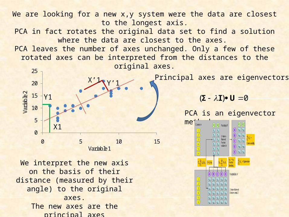
We are looking for a new x,y system were the data are closest to the longest axis.PCA in fact rotates the original data set to find a solution where the data are closest to the
axes. PCA leaves the number of axes unchanged. Only a few of these rotated axes can be
interpreted from the distances to the original axes.
We interpret the new axis on the basis of their distance (measured by their
angle) to the original axes.The new axes are the principal axes
(eigenvectors) of the dispersion matrix obtained from raw data.
X1
Y1
X’1 Y’1
0)( UIΣ
PCA is an eigenvector method
A
1
2
3
4
5
6
1
2
3
4
5
6
B C D E
z1a
z2a
z3a
z4a
z5a
z6a
z1b
z2b
z3b
z4b
z5b
z6b
z1c
z2c
z3c
z4c
z5c
z6c
z1d
z2d
z3d
z4d
z5d
z6d
z1e
z2e
z3e
z4e
z5e
z6e
F1 F2
f11
f21
f31
f41
f51
f61
f12
f22
f32
f42
f52
f62
Z-transformedData matrix Z
Z-trans-formedFactorvalues b
Cases n
Variables V
Factors F
rFV = aFVFactorloading
j2i,k
k 1
a
Communality
F1 F2
A
B
C
D
E
aa1
ab1
ac1
ad1
ae1
aa2
a22
ac2
ad2
ae2
i2k, j
k 1
a Eigenvalue
F=Z•bn
61 6k k1k 1
f z b
i
F1A F1 Ak 1
r z z
Principal axes are eigenvectors.
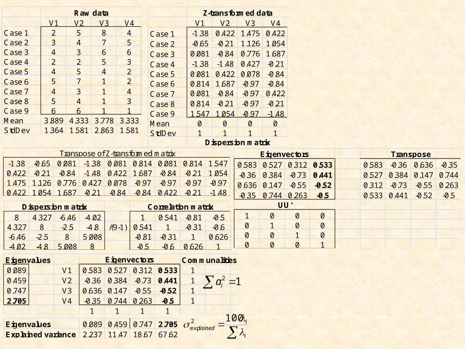
V1 V2 V3 V4Case 1 2 5 8 4Case 2 3 4 7 5Case 3 4 3 6 6Case 4 2 2 5 3Case 5 4 5 4 2Case 6 5 7 1 2Case 7 4 3 1 4Case 8 5 4 1 3Case 9 6 6 1 1Mean 3.889 4.333 3.778 3.333StdDev 1.364 1.581 2.863 1.581
Raw dataV1 V2 V3 V4
Case 1 -1.38 0.422 1.475 0.422Case 2 -0.65 -0.21 1.126 1.054Case 3 0.081 -0.84 0.776 1.687Case 4 -1.38 -1.48 0.427 -0.21Case 5 0.081 0.422 0.078 -0.84Case 6 0.814 1.687 -0.97 -0.84Case 7 0.081 -0.84 -0.97 0.422Case 8 0.814 -0.21 -0.97 -0.21Case 9 1.547 1.054 -0.97 -1.48Mean 0 0 0 0StdDev 1 1 1 1
Z-transformed data
Dispersion matrix
-1.38 -0.65 0.081 -1.38 0.081 0.814 0.081 0.814 1.5470.422 -0.21 -0.84 -1.48 0.422 1.687 -0.84 -0.21 1.0541.475 1.126 0.776 0.427 0.078 -0.97 -0.97 -0.97 -0.970.422 1.054 1.687 -0.21 -0.84 -0.84 0.422 -0.21 -1.48
Transpose of Z-transformed matrix
8 4.327 -6.46 -4.02 1 0.541 -0.81 -0.54.327 8 -2.5 -4.8 /(9-1) 0.541 1 -0.31 -0.6-6.46 -2.5 8 5.008 -0.81 -0.31 1 0.626-4.02 -4.8 5.008 8 -0.5 -0.6 0.626 1
Dispersion matrix Correlation matrix
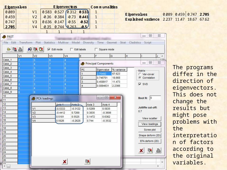
Eigenvalues Communalities0.089 V1 0.583 0.527 0.312 0.533 10.459 V2 -0.36 0.384 -0.73 0.441 10.747 V3 0.636 0.147 -0.55 -0.52 12.705 V4 -0.35 0.744 0.263 -0.5 1
1 1 1 1
Eigenvectors
Eigenvalues 0.089 0.459 0.747 2.705Explained variance 2.237 11.47 18.67 67.62
0.583 0.527 0.312 0.533 0.583 -0.36 0.636 -0.35-0.36 0.384 -0.73 0.441 0.527 0.384 0.147 0.7440.636 0.147 -0.55 -0.52 0.312 -0.73 -0.55 0.263-0.35 0.744 0.263 -0.5 0.533 0.441 -0.52 -0.5
1 0 0 00 1 0 00 0 1 00 0 0 1
UU'
Eigenvectors Transpose
12 ia
i
ilained
1002exp
Eigenvalues Communalities0.089 V1 0.583 0.527 0.312 0.533 10.459 V2 -0.36 0.384 -0.73 0.441 10.747 V3 0.636 0.147 -0.55 -0.52 12.705 V4 -0.35 0.744 0.263 -0.5 1
1 1 1 1
Eigenvectors
Eigenvalues 0.089 0.459 0.747 2.705Explained variance 2.237 11.47 18.67 67.62
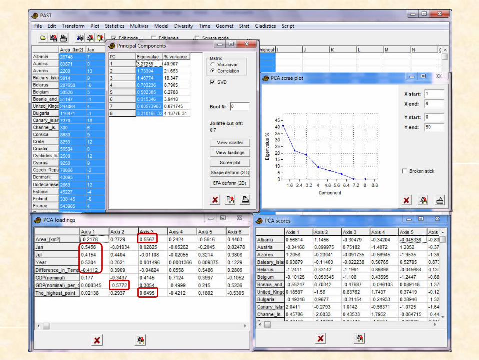
The programs differ in the direction of eigenvectors. This does not change the results but might pose problems with the interpretation of factors according to the original variables.
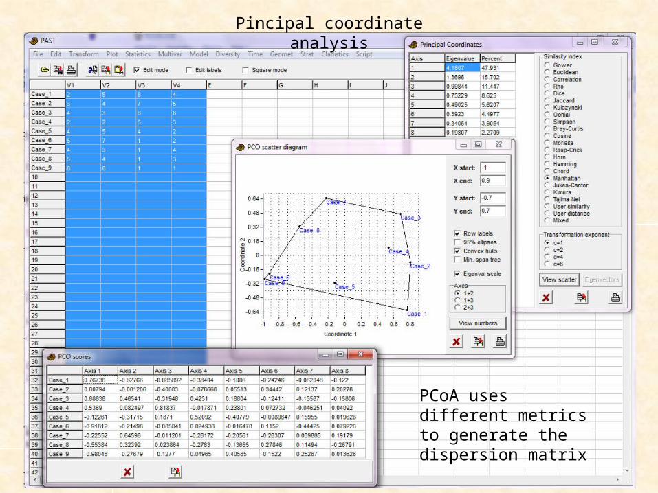
Pincipal coordinate analysis
PCoA uses different metrics to generate the dispersion matrix
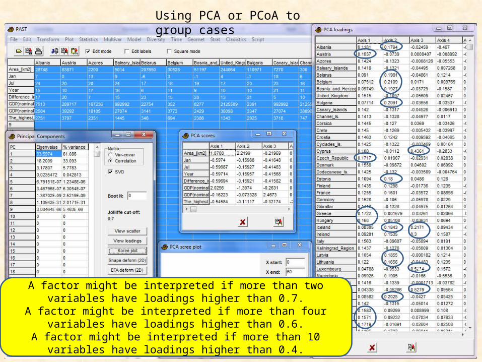
Using PCA or PCoA to group cases
vA factor might be interpreted if more than two variables have loadings
higher than 0.7.A factor might be interpreted if more than four variables have loadings
higher than 0.6.A factor might be interpreted if more than 10 variables have loadings higher
than 0.4.
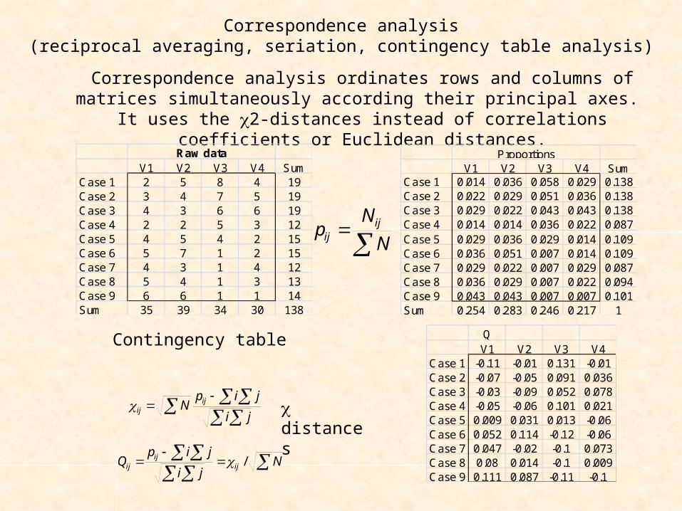
Correspondence analysis(reciprocal averaging, seriation, contingency table analysis)
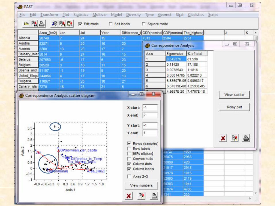
Correspondence analysis ordinates rows and columns of matrices simultaneously according their principal axes.
It uses the c2-distances instead of correlations coefficients or Euclidean distances.
V1 V2 V3 V4 SumCase 1 0.014 0.036 0.058 0.029 0.138Case 2 0.022 0.029 0.051 0.036 0.138Case 3 0.029 0.022 0.043 0.043 0.138Case 4 0.014 0.014 0.036 0.022 0.087Case 5 0.029 0.036 0.029 0.014 0.109Case 6 0.036 0.051 0.007 0.014 0.109Case 7 0.029 0.022 0.007 0.029 0.087Case 8 0.036 0.029 0.007 0.022 0.094Case 9 0.043 0.043 0.007 0.007 0.101Sum 0.254 0.283 0.246 0.217 1
ProportionsV1 V2 V3 V4 Sum
Case 1 2 5 8 4 19Case 2 3 4 7 5 19Case 3 4 3 6 6 19Case 4 2 2 5 3 12Case 5 4 5 4 2 15Case 6 5 7 1 2 15Case 7 4 3 1 4 12Case 8 5 4 1 3 13Case 9 6 6 1 1 14Sum 35 39 34 30 138
Raw data
N
Np ijij
ji
jipN ij
ij
N
ji
jipQ ij
ijij /
QV1 V2 V3 V4
Case 1 -0.11 -0.01 0.131 -0.01Case 2 -0.07 -0.05 0.091 0.036Case 3 -0.03 -0.09 0.052 0.078Case 4 -0.05 -0.06 0.101 0.021Case 5 0.009 0.031 0.013 -0.06Case 6 0.052 0.114 -0.12 -0.06Case 7 0.047 -0.02 -0.1 0.073Case 8 0.08 0.014 -0.1 0.009Case 9 0.111 0.087 -0.11 -0.1
c distances
Contingency table
V1 V2 V3 V4 SumCase 1 0.014 0.036 0.058 0.029 0.138Case 2 0.022 0.029 0.051 0.036 0.138Case 3 0.029 0.022 0.043 0.043 0.138Case 4 0.014 0.014 0.036 0.022 0.087Case 5 0.029 0.036 0.029 0.014 0.109Case 6 0.036 0.051 0.007 0.014 0.109Case 7 0.029 0.022 0.007 0.029 0.087Case 8 0.036 0.029 0.007 0.022 0.094Case 9 0.043 0.043 0.007 0.007 0.101Sum 0.254 0.283 0.246 0.217 1
Proportions
QV1 V2 V3 V4
Case 1 -0.11 -0.01 0.131 -0.01Case 2 -0.07 -0.05 0.091 0.036Case 3 -0.03 -0.09 0.052 0.078Case 4 -0.05 -0.06 0.101 0.021Case 5 0.009 0.031 0.013 -0.06Case 6 0.052 0.114 -0.12 -0.06Case 7 0.047 -0.02 -0.1 0.073Case 8 0.08 0.014 -0.1 0.009Case 9 0.111 0.087 -0.11 -0.1
V1 V2 V3 V4 SumCase 1 2 5 8 4 19Case 2 3 4 7 5 19Case 3 4 3 6 6 19Case 4 2 2 5 3 12Case 5 4 5 4 2 15Case 6 5 7 1 2 15Case 7 4 3 1 4 12Case 8 5 4 1 3 13Case 9 6 6 1 1 14Sum 35 39 34 30 138
Raw data-0.11 -0.07 -0.03 -0.05 0.009 0.052 0.047 0.08 0.111-0.01 -0.05 -0.09 -0.06 0.031 0.114 -0.02 0.014 0.0870.131 0.091 0.052 0.101 0.013 -0.12 -0.1 -0.1 -0.11-0.01 0.036 0.078 0.021 -0.06 -0.06 0.073 0.009 -0.1
Q'Q0.044 0.027 -0.06 -0.020.027 0.037 -0.04 -0.03-0.06 -0.04 0.086 0.018-0.02 -0.03 0.018 0.03
Transpose of Q
Case 1Case 2Case 3Case 4Case 5Case 6Case 7Case 8Case 9SumV1 2 3 4 2 4 5 4 5 6 35V2 5 4 3 2 5 7 3 4 6 39V3 8 7 6 5 4 1 1 1 1 34V4 4 5 6 3 2 2 4 3 1 30
Sum 19 19 19 12 15 15 12 13 14 138
Transpose of raw data matrix
Eigenvalues0 0.504 0.663 0.225 0.506
0.00459 0.532 -0.55 -0.49 0.4120.0348 0.496 0.301 -0.39 -0.710.15743 0.466 -0.41 0.741 -0.26
Eigenvectors Eigenvalues0 0.408 0.408 0.408 0.408 0.408 0.408 0.346 0.394 0.3840 -0.82 -0.82 -0.82 -0.82 -0.82 -0.82 0.096 2E-04 0.330 0.408 0.408 0.408 0.408 0.408 0.408 -0.15 -0.39 0.2750 0 0 0 0 0 0 -0.35 0.023 0.3270 0 0 0 0 0 0 -0.25 0.338 -0.060 0 0 0 0 0 0 0.588 0.223 -0.44
0.005 0 0 0 0 0 0 0.268 -0.6 -0.170.035 0 0 0 0 0 0 -0.15 -0.31 -0.30.157 0 0 0 0 0 0 -0.47 0.257 -0.5
Eigenvectors
-0.8-0.6-0.4-0.2
00.20.40.60.8
1
-1 -0.5 0 0.5 1Seco
nd a
xis
First axis
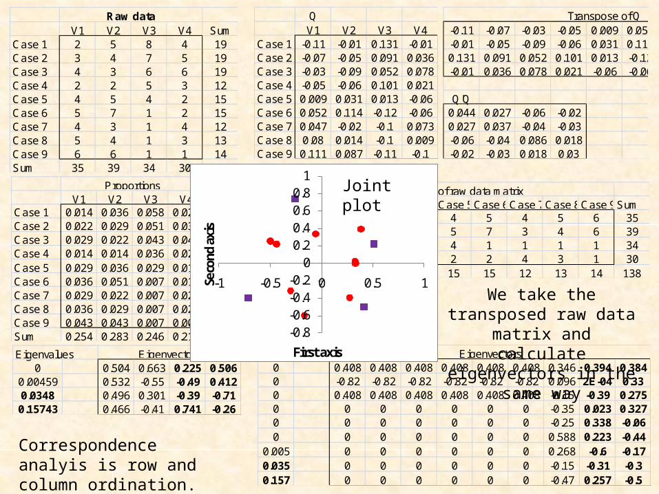
We take the transposed raw data matrix and calculate eigenvectors in the same
way
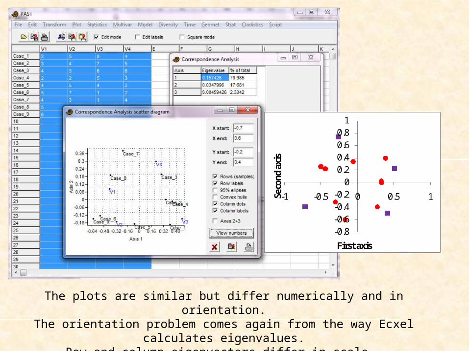
Correspondence analyis is row and column ordination.
Joint plot
-0.8-0.6-0.4-0.2
00.20.40.60.8
1
-1 -0.5 0 0.5 1Seco
nd a
xis
First axis
The plots are similar but differ numerically and in orientation.The orientation problem comes again from the way Ecxel calculates eigenvalues.
Row and column eigenvectors differ in scale. For a joint plot the vectors have to be rescaled.
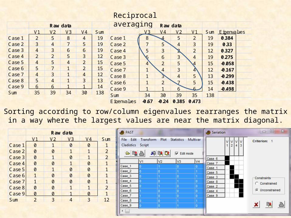
Reciprocal averaging
V3 V4 V2 V1 Sum EigenvaluesCase 1 8 4 5 2 19 0.384Case 2 7 5 4 3 19 0.33Case 4 5 3 2 2 12 0.327Case 3 6 6 3 4 19 0.275Case 5 4 2 5 4 15 -0.058Case 7 1 4 3 4 12 -0.167Case 8 1 3 4 5 13 -0.299Case 6 1 2 7 5 15 -0.438Case 9 1 1 6 6 14 -0.498Sum 34 30 39 35 138Eigenvalues -0.67 -0.24 0.385 0.473
Raw dataV1 V2 V3 V4 Sum
Case 1 2 5 8 4 19Case 2 3 4 7 5 19Case 3 4 3 6 6 19Case 4 2 2 5 3 12Case 5 4 5 4 2 15Case 6 5 7 1 2 15Case 7 4 3 1 4 12Case 8 5 4 1 3 13Case 9 6 6 1 1 14Sum 35 39 34 30 138
Raw data
V1 V2 V3 V4 SumCase 1 0 1 0 0 1Case 2 0 0 1 1 2Case 3 0 1 0 1 2Case 4 0 0 1 0 1Case 5 0 1 0 0 1Case 6 1 0 0 0 1Case 7 1 0 0 0 1Case 8 0 0 1 1 2Case 9 0 0 1 0 1Sum 2 3 4 3 12
Raw data
Sorting according to row/column eigenvalues rearranges the matrix in a way where the largest values are near the matrix diagonal.
V1 V2 V3 V4 SumCase 1 0 1 0 0 1Case 2 0 0 1 1 2Case 3 0 1 0 1 2Case 4 0 0 1 0 1Case 5 0 1 0 0 1Case 6 1 0 0 0 1Case 7 1 0 0 0 1Case 8 0 0 1 1 2Case 9 0 0 1 0 1Sum 2 3 4 3 12
Raw data
V3 V1 V4 V2 Sum 1 1 2 3Case 4 1 0 0 0 1 0.063 -1.491 -1.12 -1.155 -0.896 -0.939Case 9 1 0 0 0 1 0.063 -1.491 -1.12 -1.155 -0.896 -0.939Case 6 0 1 0 0 1 0.408 -0.195 -0.47 -0.431 -0.562 -0.577Case 7 0 1 0 0 1 0.408 -0.195 -0.47 -0.431 -0.562 -0.577Case 2 1 0 1 0 2 0.486 0.099 -0.343 -0.288 -0.404 -0.406Case 8 1 0 1 0 2 0.486 0.099 -0.343 -0.288 -0.404 -0.406Case 3 0 0 1 1 2 0.808 1.311 0.795 0.981 0.729 0.819Case 1 0 0 0 1 1 0.708 0.933 1.156 1.384 1.369 1.512Case 5 0 0 0 1 1 0.708 0.933 1.156 1.384 1.369 1.512Sum 4 2 3 3 12 Mean 0.46 -0.084 -0.028
StdDev 0.266 0.896 0.924Mean StDev
1 0.063 0.408 0.909 0.7082 0.275 0.408 0.594 0.741 0.504 0.2052 -1.12 -0.47 0.435 1.1563 -0.731 -0.47 0.037 1.035 -0.032 0.783 -0.896 -0.562 0.089 1.3694 -0.65 -0.562 -0.026 1.156 -0.021 0.8314 -0.757 -0.651 -0.007 1.415
Raw data
=los()
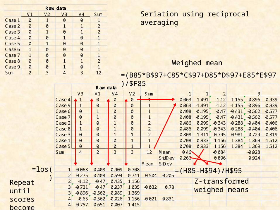
=(B85*B$97+C85*C$97+D85*D$97+E85*E$97)/$F85
=(H85-H$94)/H$95
Seriation using reciprocal averaging
Repeat until scores become stable
Weighed mean
Z-transformed weighed means
Related Documents