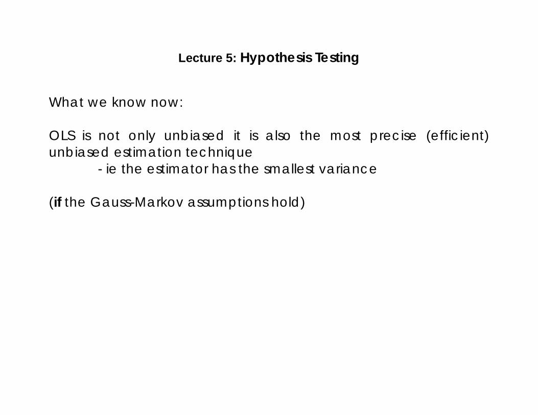
Lecture 5: Hypothesis Testing What we know now: OLS is not only unbiased it is also the most precise (efficient) unbiased estimation technique - ie the estimator has the smallest variance (if the Gauss-Markov assumptions hold)

Welcome message from author
This document is posted to help you gain knowledge. Please leave a comment to let me know what you think about it! Share it to your friends and learn new things together.
Transcript
Lecture 5: Hypothesis Testing
What we know now: OLS is not only unbiased it is also the most precise (efficient) unbiased estimation technique
- ie the estimator has the smallest variance (if the Gauss-Markov assumptions hold)
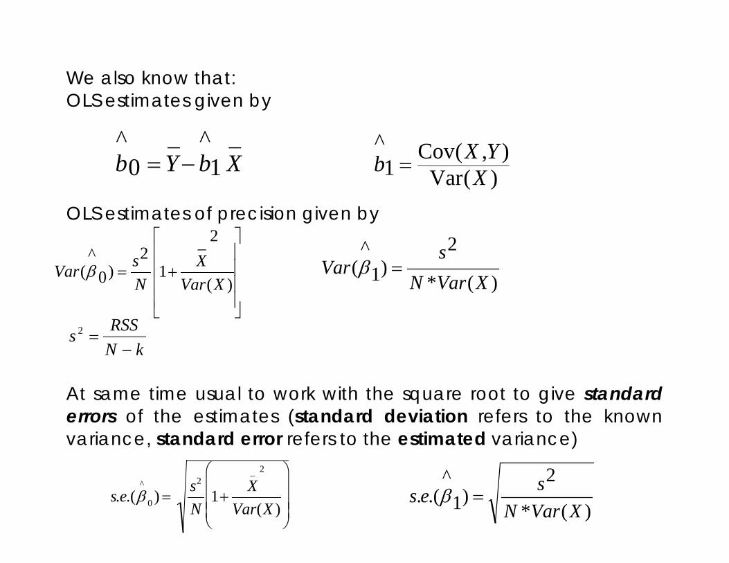
We also know that: OLS estimates given by OLS estimates of precision given by
kNRSSs
−=2
At same time usual to work with the square root to give standard errors of the estimates (standard deviation refers to the known variance, standard error refers to the estimated variance)
_1
^_0
^XbYb −= )(Var
),(Cov1
^X
YXb =
+=)(
2_
12
)0^
(XVar
XNsVar β )(*
2)1
^(
XVarNs
Var =β
s.e.(β^
0 ) =s2
N1+
X_ 2
Var(X )
)(*
2)1
^.(.
XVarNses =β
Now need to learn how to test hypotheses about whether the values of the individual estimates we get are consistent with the way we think the world may work Eg if we estimate the model by OLS C=b0 + b1Y + u and the estimated coefficient on income is b1 = 0.9 is this consistent with what we think the marginal propensity to consume should be? Now common (economic) sense can help here, but in itself it is not rigorous (or impartial) enough which is where hypothesis testing comes in
Hypothesis Testing If wish to make inferences about how close an estimated value is to a hypothesised value or even to say whether the influence of a variable is not simply the result of statistical chance (the estimates being based on a sample and so subject to random fluctuations) then need to make one additional assumption about the behaviour of the (true, unobserved) residuals in the model
Hypothesis Testing If wish to make inferences about how close an estimated value is to a hypothesised value or even to say whether the influence of a variable is not simply the result of statistical chance then need to make one additional assumption about the behaviour of the (true, unobserved) residuals in the model (the estimates being based on a sample and so subject to random fluctuations) then need to make one additional assumption about the behaviour of the (true, unobserved) residuals in the model We know already that ui ~ (0, σ2u) ie true residuals assumed to have a mean of zero and variance σ2u
Hypothesis Testing If wish to make inferences about how close an estimated value is to a hypothesised value or even to say whether the influence of a variable is not simply the result of statistical chance then need to make one additional assumption about the behaviour of the (true, unobserved) residuals in the model (the estimates being based on a sample and so subject to random fluctuations) then need to make one additional assumption about the behaviour of the (true, unobserved) residuals in the model We know already that ui ~ (0, σ2u) ie true residuals assumed to have a mean of zero and variance σ2u
Now assume additionally that residuals follow a Normal distribution
Now assume additionally that residuals follow a Normal distribution
ui ~N(0, σ2u)
Now assume additionally that residuals follow a Normal distribution
ui ~N(0, σ2u)
(Since residuals capture influence of many unobserved (random) variables, can use Central Limit Theorem which says that the sum of a large set of random variables will have a normal distribution)
If u is normal, then it is easy to show that the OLS coefficients (which are a linear function of u) are also normally distributed with the means and variances that we derived earlier. So
))(,(~ 0^
00^
βββ VarN and ))(,(~ 1^
11^
βββ VarN
If u is normal, then it is easy to show that the OLS coefficients (which are a linear function of u) are also normally distributed with the means and variances that we derived earlier. So
))(,(~ 0^
00^
βββ VarN and ))(,(~ 1^
11^
βββ VarN Why is that any use to us?
If a variable is normally distributed we know that it is Symmetric

If a variable is normally distributed we know that it is Symmetric
If a variable is normally distributed we know that it is Symmetric centred on its mean (use the symbol μ) and that the symmetry pattern is such that: 66% of values lie within mean ±1*standard deviation
If a variable is normally distributed we know that it is Symmetric centred on its mean (use the symbol μ ) and that the symmetry pattern is such that: 66% of values lie within mean ±1*standard deviation (use the symbol σ )
If a variable is normally distributed we know that it is Symmetric centred on its mean (use the symbol μ) and that the symmetry pattern is such that: 66% of values lie within mean ±1*standard deviation (use the symbol σ ) 95% of values lie within mean ±1.96*σ
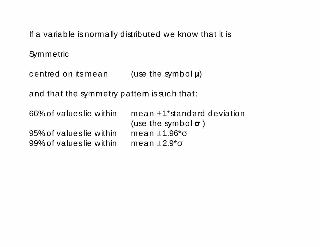
If a variable is normally distributed we know that it is Symmetric centred on its mean (use the symbol μ) and that the symmetry pattern is such that: 66% of values lie within mean ±1*standard deviation (use the symbol σ ) 95% of values lie within mean ±1.96*σ 99% of values lie within mean ±2.9*σ
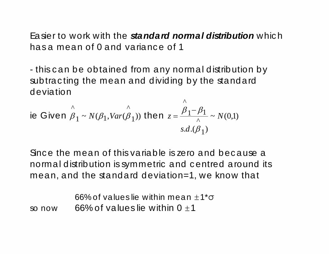
Easier to work with the standard normal distribution which has a mean (μ) of 0 and variance (σ2u ) of 1
ui ~N(0, 1)
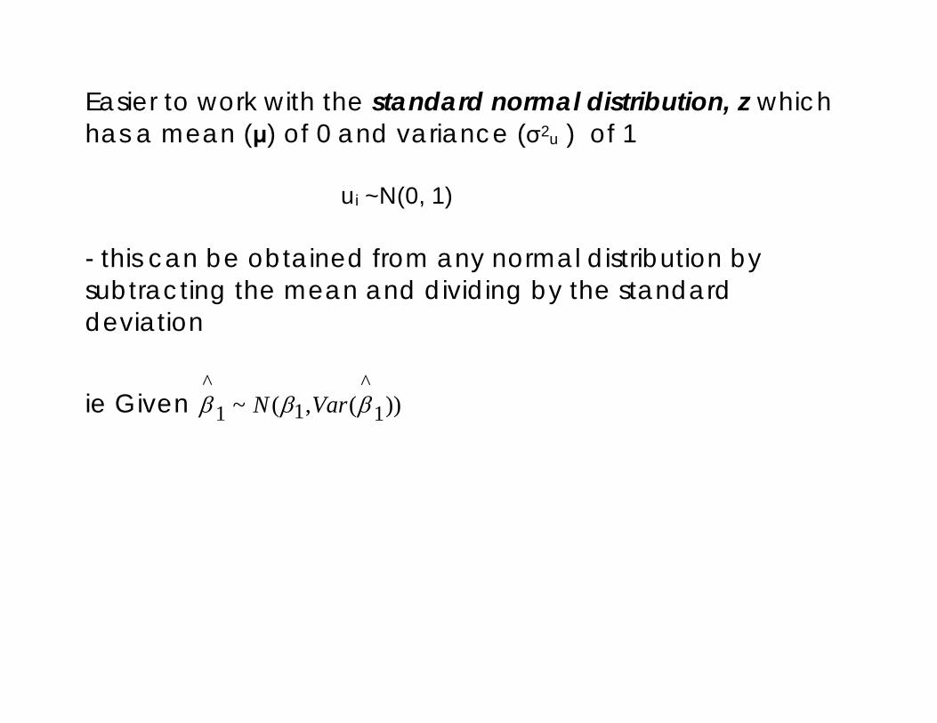
Easier to work with the standard normal distribution, z which has a mean (μ) of 0 and variance (σ2u ) of 1
ui ~N(0, 1) - this can be obtained from any normal distribution by subtracting the mean and dividing by the standard deviation
Easier to work with the standard normal distribution, z which has a mean (μ) of 0 and variance (σ2u ) of 1
ui ~N(0, 1) - this can be obtained from any normal distribution by subtracting the mean and dividing by the standard deviation
ie Given ))(,(~ 1^
11^
βββ VarN
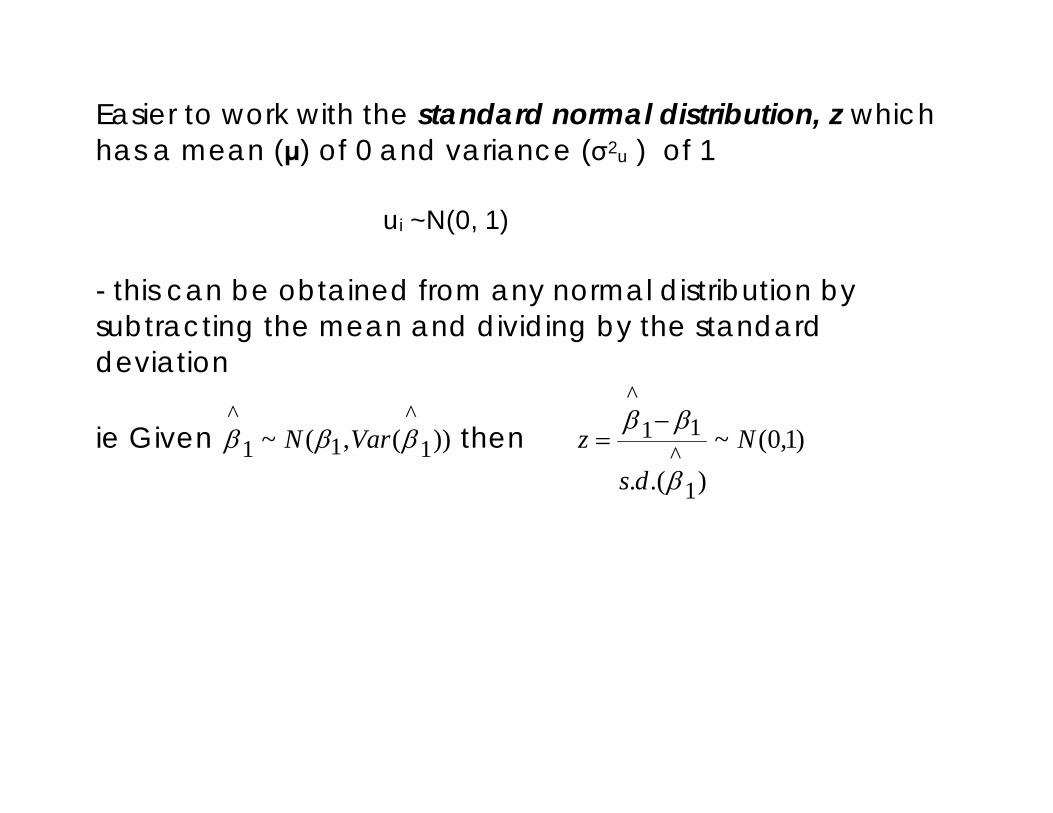
Easier to work with the standard normal distribution, z which has a mean (μ) of 0 and variance (σ2u ) of 1
ui ~N(0, 1) - this can be obtained from any normal distribution by subtracting the mean and dividing by the standard deviation
ie Given ))(,(~ 1^
11^
βββ VarN then )1,0(~).(. 1
^11
^
Nds
zβ
ββ −=
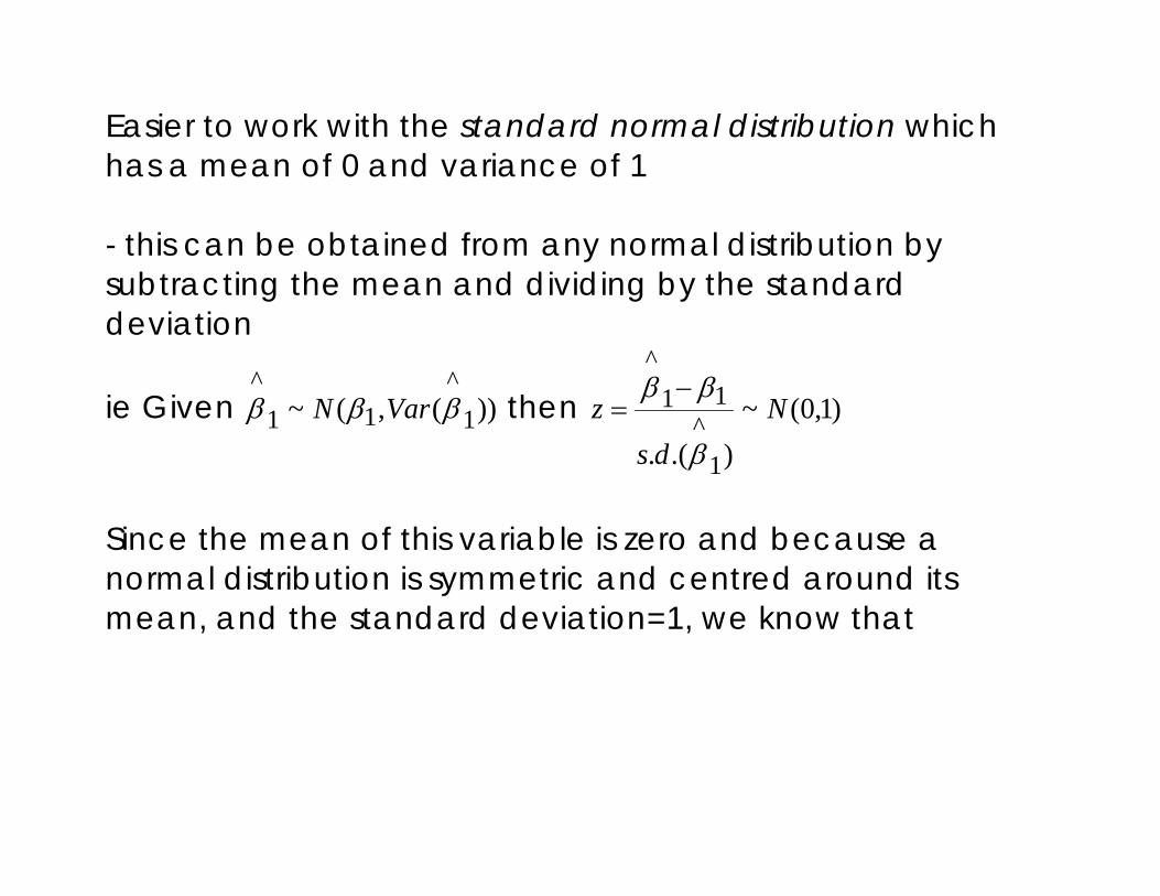
Easier to work with the standard normal distribution which has a mean of 0 and variance of 1 - this can be obtained from any normal distribution by subtracting the mean and dividing by the standard deviation
ie Given ))(,(~ 1^
11^
βββ VarN then )1,0(~).(. 1
^11
^
Nds
zβ
ββ −=
Since the mean of this variable is zero and because a normal distribution is symmetric and centred around its mean, and the standard deviation=1, we know that
66% of values lie within mean ±1*σ
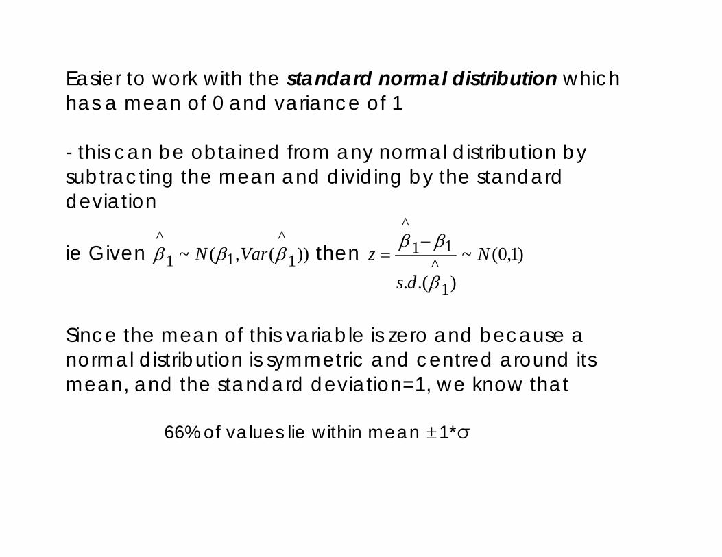
Easier to work with the standard normal distribution which has a mean of 0 and variance of 1 - this can be obtained from any normal distribution by subtracting the mean and dividing by the standard deviation
ie Given ))(,(~ 1^
11^
βββ VarN then )1,0(~).(. 1
^11
^
Nds
zβ
ββ −=
Since the mean of this variable is zero and because a normal distribution is symmetric and centred around its mean, and the standard deviation=1, we know that
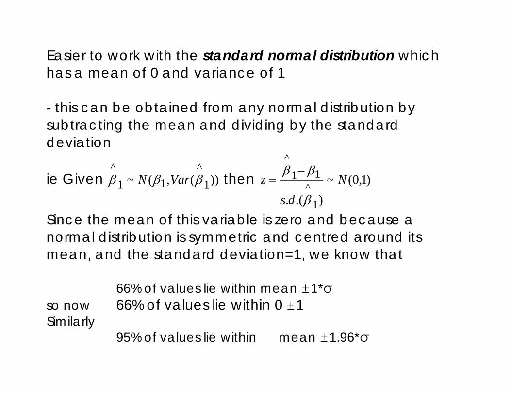
66% of values lie within mean ±1*σ so now 66% of values lie within 0 ±1
Easier to work with the standard normal distribution which has a mean of 0 and variance of 1 - this can be obtained from any normal distribution by subtracting the mean and dividing by the standard deviation
ie Given ))(,(~ 1^
11^
βββ VarN then )1,0(~).(. 1
^11
^
Nds
zβ
ββ −=
Since the mean of this variable is zero and because a normal distribution is symmetric and centred around its mean, and the standard deviation=1, we know that
66% of values lie within mean ±1*σ so now 66% of values lie within 0 ±1 Similarly
95% of values lie within mean ±1.96*σ

99% of values lie within mean ±2.9*σ
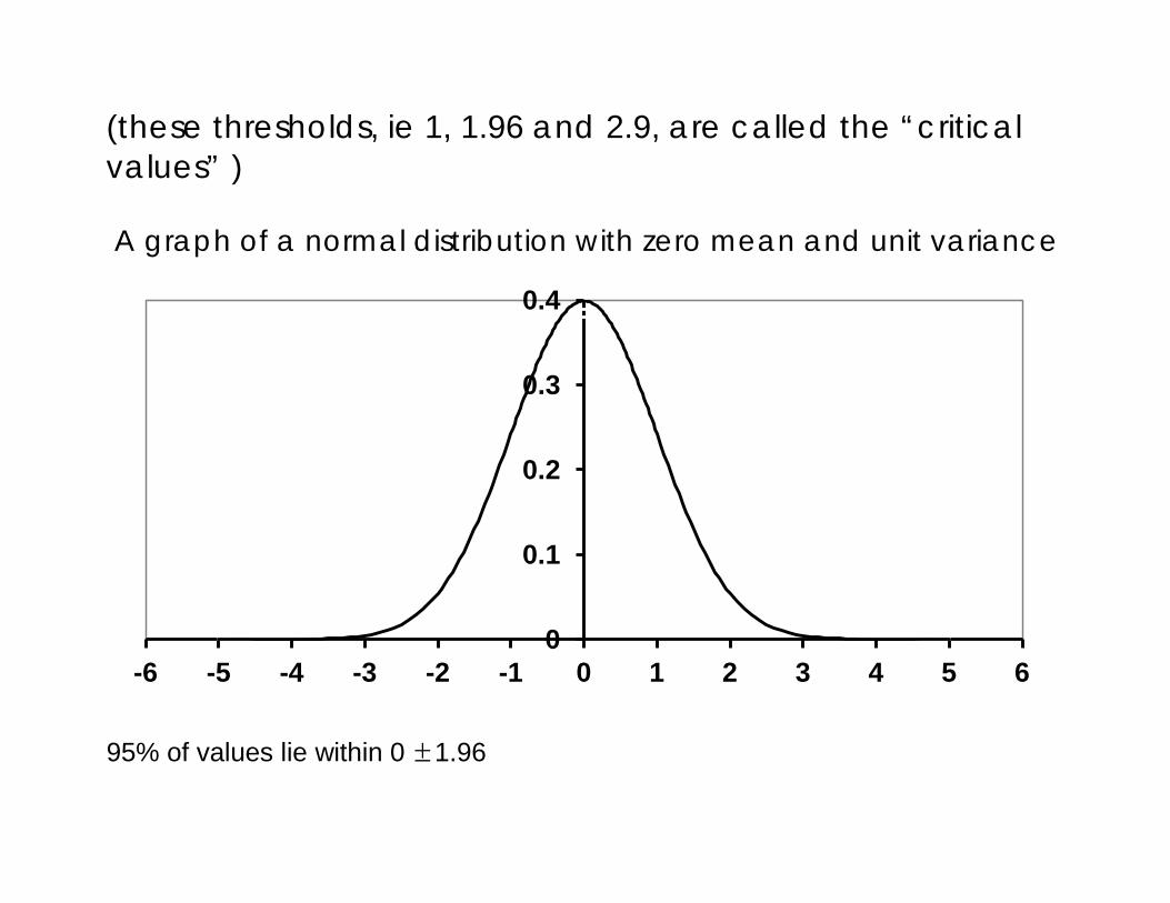
(these thresholds, ie 1, 1.96 and 2.9, are called the “critical values” ) A graph of a normal distribution with zero mean and unit variance
95% of values lie within 0 ±1.96
0
0.1
0.2
0.3
0.4
-6 -5 -4 -3 -2 -1 0 1 2 3 4 5 6
so the critical value for the 95% significance level is 1.96 Can use all this to test hypotheses about the values of individual coefficients Testing A Hypothesis Relating To A Regression Coefficient Model: Y = β0 + β1 X + u
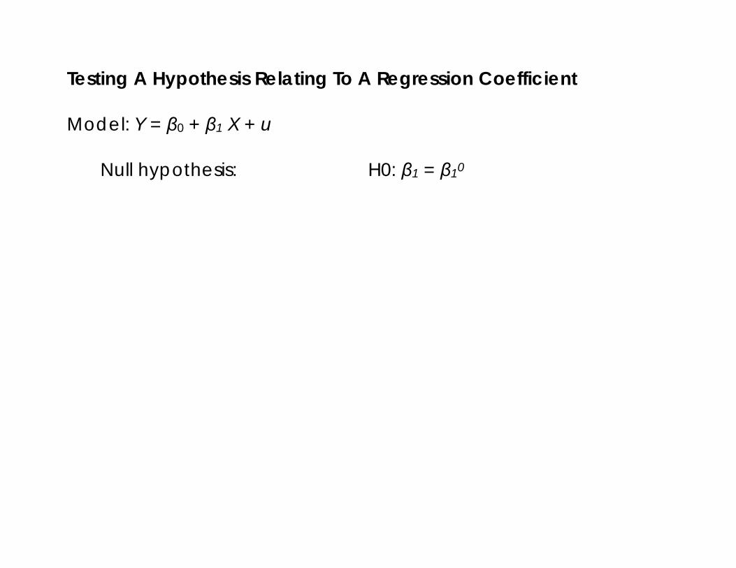
Testing A Hypothesis Relating To A Regression Coefficient Model: Y = β0 + β1 X + u Null hypothesis: H0: β1 = β10
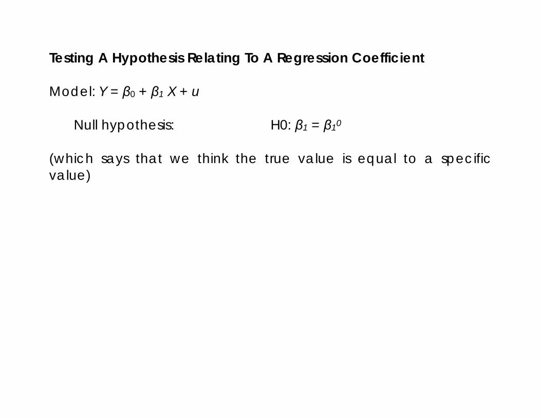
Testing A Hypothesis Relating To A Regression Coefficient Model: Y = β0 + β1 X + u Null hypothesis: H0: β1 = β10
(which says that we think the true value is equal to a specific value)
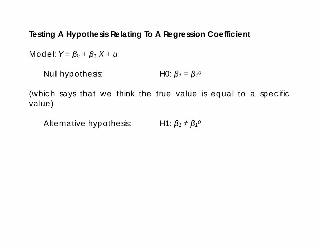
Testing A Hypothesis Relating To A Regression Coefficient Model: Y = β0 + β1 X + u Null hypothesis: H0: β1 = β10
(which says that we think the true value is equal to a specific value) Alternative hypothesis: H1: β1 ≠ β10
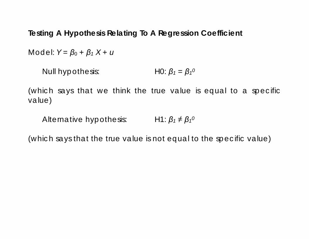
Testing A Hypothesis Relating To A Regression Coefficient Model: Y = β0 + β1 X + u Null hypothesis: H0: β1 = β10
(which says that we think the true value is equal to a specific value) Alternative hypothesis: H1: β1 ≠ β10
(which says that the true value is not equal to the specific value)

Testing A Hypothesis Relating To A Regression Coefficient Model: Y = β0 + β1 X + u Null hypothesis: H0: β1 = β10
(which says that we think the true value is equal to a specific value) Alternative hypothesis: H1: β1 ≠ β10
(which says that the true value is not equal to the specific value) But because OLS is only an estimate we have to allow for the uncertainty in the estimate – as captured by its standard error
Testing A Hypothesis Relating To A Regression Coefficient Model: Y = β0 + β1 X + u Null hypothesis: H0: β1 = β10
(which says that we think the true value is equal to a specific value) Alternative hypothesis: H1: β1 ≠ β10
(which says that the true value is not equal to the specific value) But because OLS is only an estimate we have to allow for the uncertainty in the estimate – as captured by its standard error Implicitly the variance says the estimate may be centred on this value but because this is only an estimate and not the truth, there is a possible range of other plausible values associated with it
Testing A Hypothesis Relating To A Regression Coefficient The most common hypothesis to be tested (and most regression packages default hypothesis) is that the true value of the coefficient is zero
Testing A Hypothesis Relating To A Regression Coefficient The most common hypothesis to be tested (and most regression packages default hypothesis) is that the true value of the coefficient is zero
- Which is the same thing as saying the effect of the variable is zero Since β1 = dY/dX
Testing A Hypothesis Relating To A Regression Coefficient The most common hypothesis to be tested (and most regression packages default hypothesis) is that the true value of the coefficient is zero
- Which is the same thing as saying the effect of the variable is zero Since β1 = dY/dX
Example Cons = β0 + β1Income + u
Testing A Hypothesis Relating To A Regression Coefficient The most common hypothesis to be tested (and most regression packages default hypothesis) is that the true value of the coefficient is zero
- Which is the same thing as saying the effect of the variable is zero Since β1 = dY/dX
Example Cons = β0 + β1Income + u Null hypothesis: H0: β1 = 0
Testing A Hypothesis Relating To A Regression Coefficient The most common hypothesis to be tested (and most regression packages default hypothesis) is that the true value of the coefficient is zero
- Which is the same thing as saying the effect of the variable is zero Since β1 = dY/dX
Example Cons = β0 + β1Income + u Null hypothesis: H0: β1 = 0 Alternative hypothesis: H1: β1 ≠ 0
Testing A Hypothesis Relating To A Regression Coefficient The most common hypothesis to be tested (and most regression packages default hypothesis) is that the true value of the coefficient is zero
- Which is the same thing as saying the effect of the variable is zero Since β1 = dY/dX
Example Cons = β0 + β1Income + u Null hypothesis: H0: β1 = 0 Alternative hypothesis: H1: β1 ≠ 0 and this time β1 = dCons/dIncome
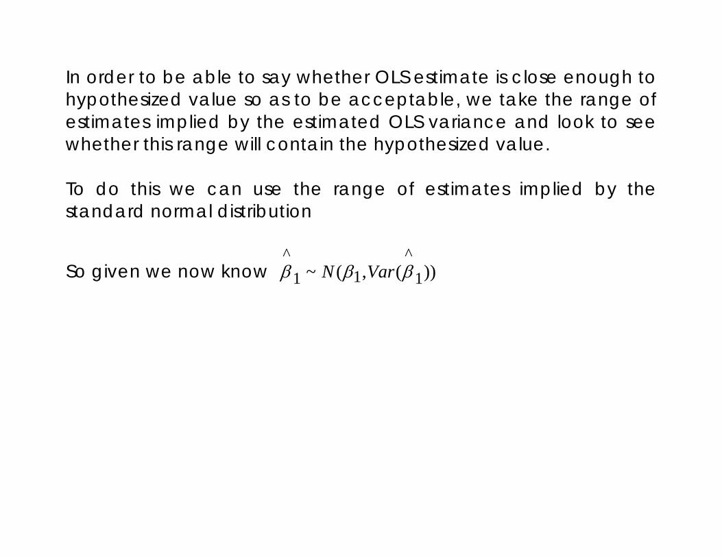
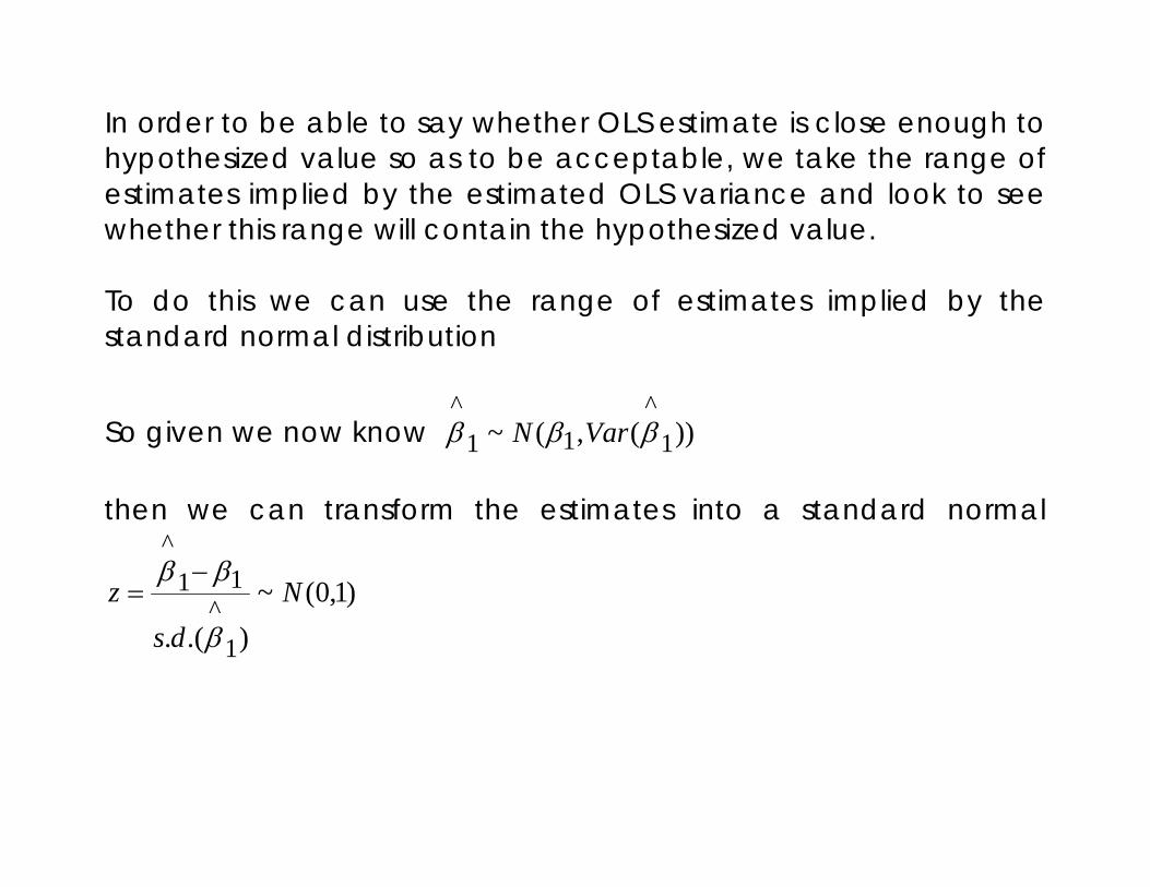
In order to be able to say whether OLS estimate is close enough to hypothesized value so as to be acceptable, we take the range of estimates implied by the estimated OLS variance and look to see whether this range will contain the hypothesized value.

In order to be able to say whether OLS estimate is close enough to hypothesized value so as to be acceptable, we take the range of estimates implied by the estimated OLS variance and look to see whether this range will contain the hypothesized value. To do this we can use the range of estimates implied by the standard normal distribution
In order to be able to say whether OLS estimate is close enough to hypothesized value so as to be acceptable, we take the range of estimates implied by the estimated OLS variance and look to see whether this range will contain the hypothesized value. To do this we can use the range of estimates implied by the standard normal distribution
So given we now know ))(,(~ 1^
11^
βββ VarN
In order to be able to say whether OLS estimate is close enough to hypothesized value so as to be acceptable, we take the range of estimates implied by the estimated OLS variance and look to see whether this range will contain the hypothesized value. To do this we can use the range of estimates implied by the standard normal distribution
So given we now know ))(,(~ 1^
11^
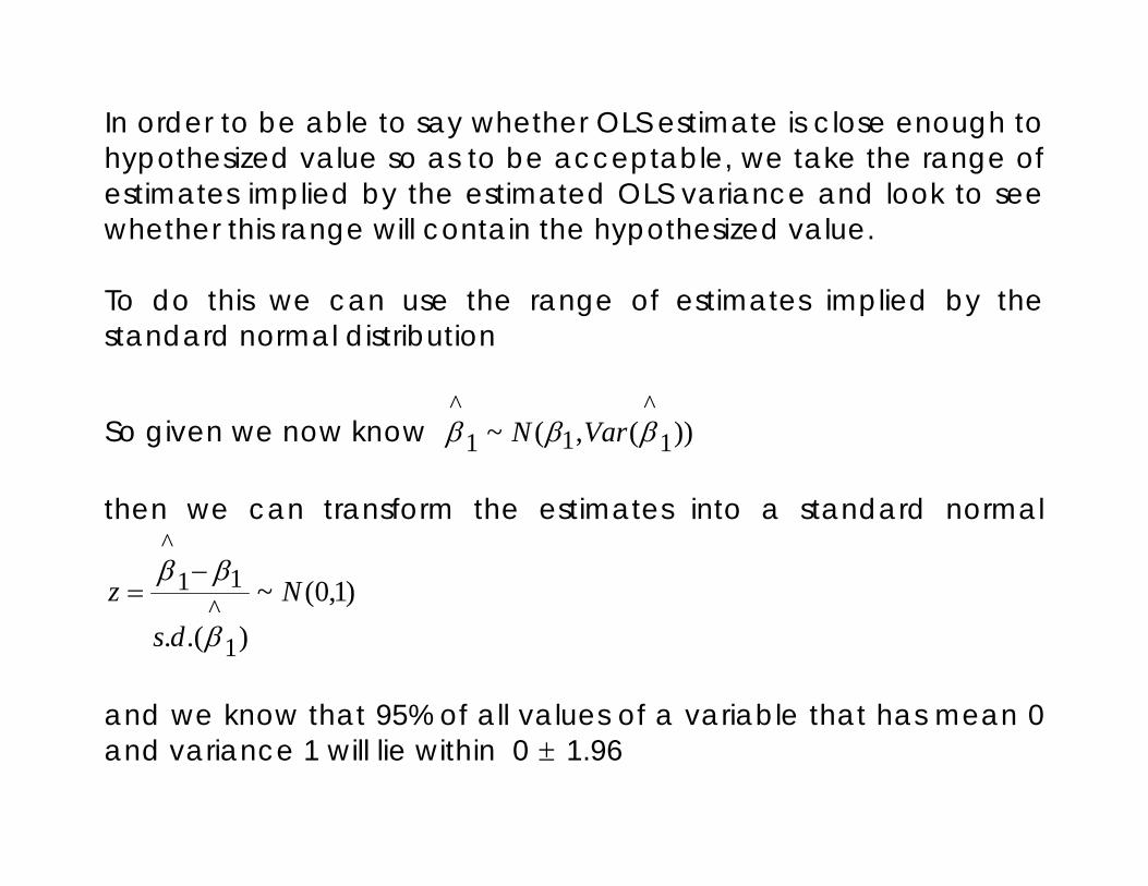
βββ VarN then we can transform the estimates into a standard normal
)1,0(~).(. 1
^11
^
Nds
zβ
ββ −=
In order to be able to say whether OLS estimate is close enough to hypothesized value so as to be acceptable, we take the range of estimates implied by the estimated OLS variance and look to see whether this range will contain the hypothesized value. To do this we can use the range of estimates implied by the standard normal distribution
So given we now know ))(,(~ 1^
11^
βββ VarN then we can transform the estimates into a standard normal
)1,0(~).(. 1
^11
^
Nds
zβ
ββ −=
and we know that 95% of all values of a variable that has mean 0 and variance 1 will lie within 0 ± 1.96
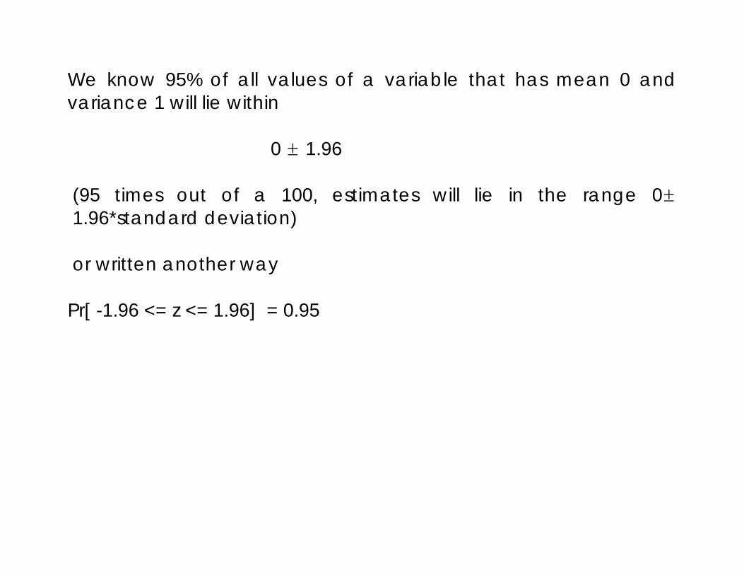
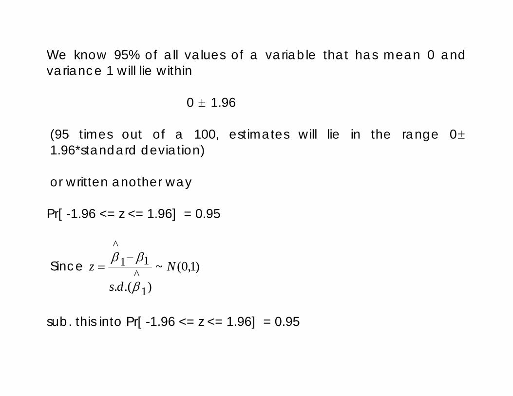
We know 95% of all values of a variable that has mean 0 and variance 1 will lie within
0 ± 1.96
(95 times out of a 100, estimates will lie in the range 0±1.96*standard deviation) or written another way
We know 95% of all values of a variable that has mean 0 and variance 1 will lie within
0 ± 1.96
(95 times out of a 100, estimates will lie in the range 0±1.96*standard deviation) or written another way Pr[ -1.96 <= z <= 1.96] = 0.95
We know 95% of all values of a variable that has mean 0 and variance 1 will lie within
0 ± 1.96
(95 times out of a 100, estimates will lie in the range 0±1.96*standard deviation) or written another way Pr[ -1.96 <= z <= 1.96] = 0.95
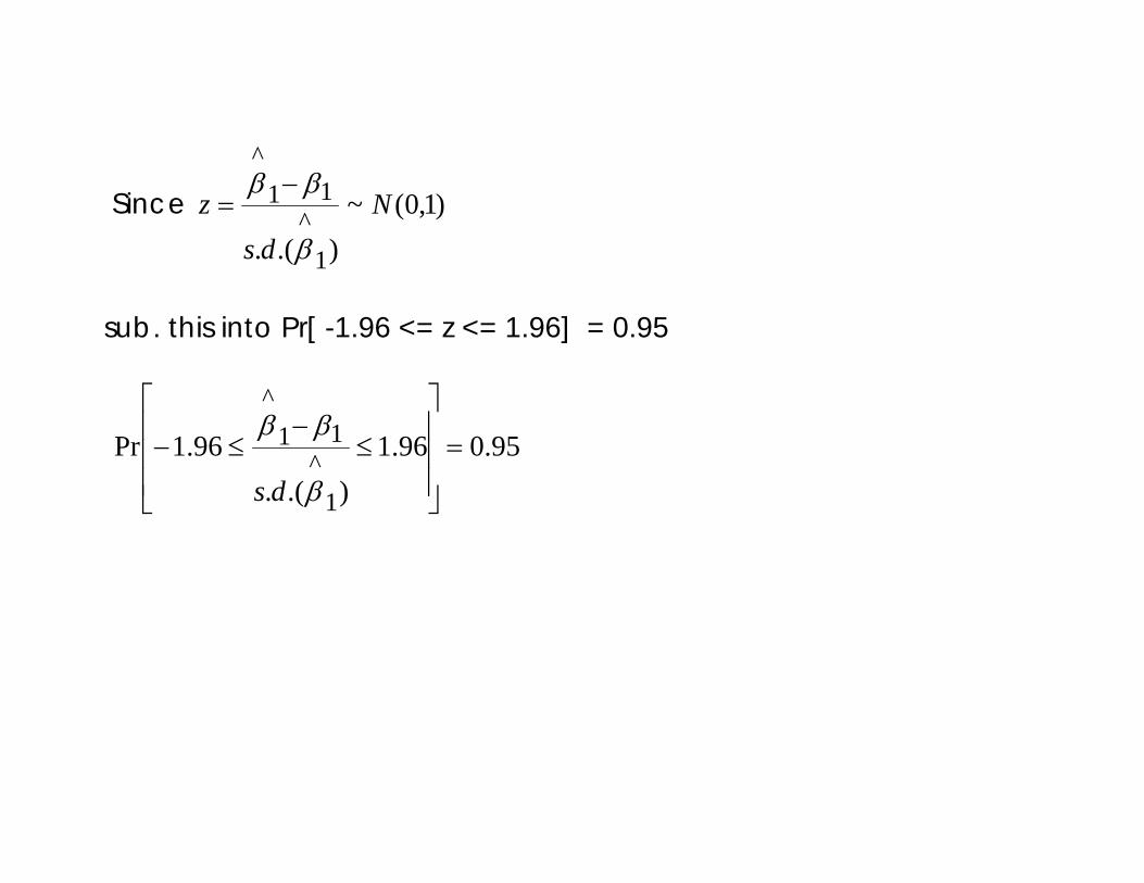
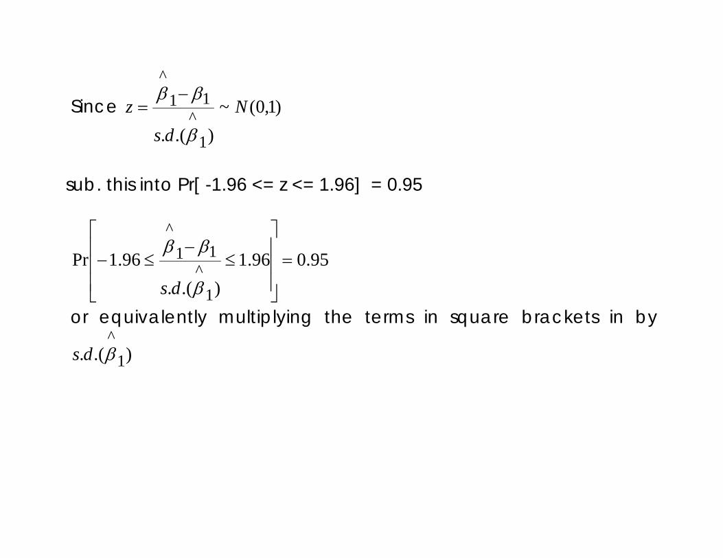
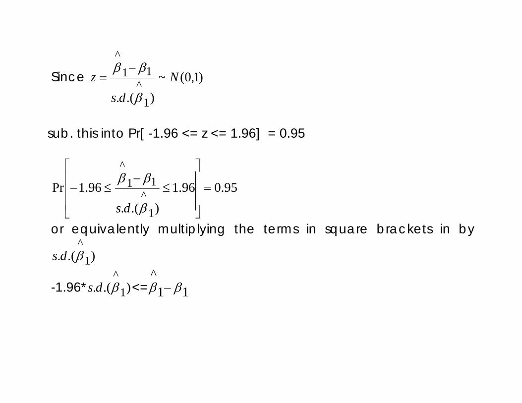
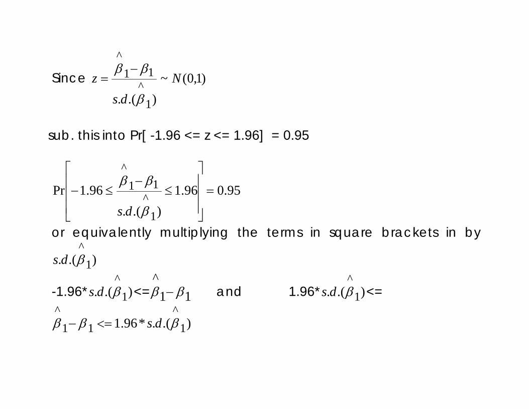
Since )1,0(~).(. 1
^11
^
Nds
zβ
ββ −=
sub. this into Pr[ -1.96 <= z <= 1.96] = 0.95
Since )1,0(~).(. 1
^11
^
Nds
zβ
ββ −=
sub. this into Pr[ -1.96 <= z <= 1.96] = 0.95
95.096.1).(.
96.1Pr
1^
11^
=
≤−
≤−
β
ββ
ds
Since )1,0(~).(. 1
^11
^
Nds
zβ
ββ −=
sub. this into Pr[ -1.96 <= z <= 1.96] = 0.95
95.096.1).(.
96.1Pr
1^
11^
=
≤−
≤−
β
ββ
ds
or equivalently multiplying the terms in square brackets in by
).(. 1^βds
Since )1,0(~).(. 1
^11
^
Nds
zβ
ββ −=
sub. this into Pr[ -1.96 <= z <= 1.96] = 0.95
95.096.1).(.
96.1Pr
1^
11^
=
≤−
≤−
β
ββ
ds
or equivalently multiplying the terms in square brackets in by
).(. 1^βds
-1.96* ).(. 1^βds <= 11
^ββ −

Since )1,0(~).(. 1
^11
^
Nds
zβ
ββ −=
sub. this into Pr[ -1.96 <= z <= 1.96] = 0.95
95.096.1).(.
96.1Pr
1^
11^
=
≤−
≤−
β
ββ
ds
or equivalently multiplying the terms in square brackets in by
).(. 1^βds
-1.96* ).(. 1^βds <= 11
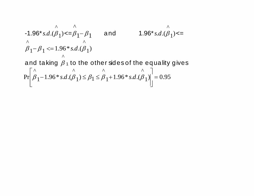
^ββ − and 1.96* ).(. 1
^βds <=
).(.*96.1 1^
11^
βββ ds<=−
Since )1,0(~).(. 1
^11
^
Nds
zβ
ββ −=
sub. this into Pr[ -1.96 <= z <= 1.96] = 0.95
95.096.1).(.
96.1Pr
1^
11^
=
≤−
≤−
β
ββ
ds
or equivalently multiplying the terms in square brackets in by
).(. 1^βds
-1.96* ).(. 1^βds <= 11
^ββ − and 1.96* ).(. 1
^βds <=
).(.*96.1 1^
11^
βββ ds<=−
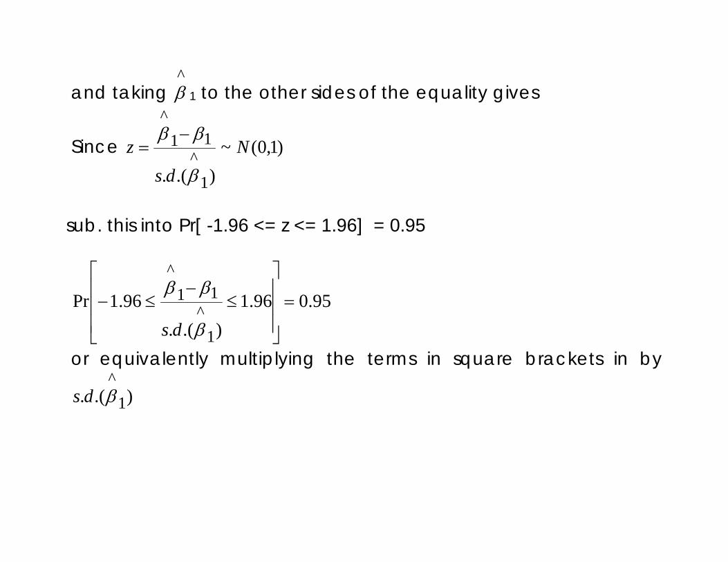
and taking ^β 1 to the other sides of the equality gives
Since )1,0(~).(. 1
^11
^
Nds
zβ
ββ −=
sub. this into Pr[ -1.96 <= z <= 1.96] = 0.95
95.096.1).(.
96.1Pr
1^
11^
=
≤−
≤−
β
ββ
ds
or equivalently multiplying the terms in square brackets in by
).(. 1^βds
-1.96* ).(. 1^βds <= 11
^ββ − and 1.96* ).(. 1
^βds <=
).(.*96.1 1^
11^
βββ ds<=−
and taking ^β 1 to the other sides of the equality gives
95.0).(.*96.1).(.*96.1Pr 1^
1^
11^
1^
=
+≤≤− βββββ dsds
95.0).(.*96.1).(.*96.1Pr 1^
1^
11^
1^
=
+≤≤− βββββ dsds
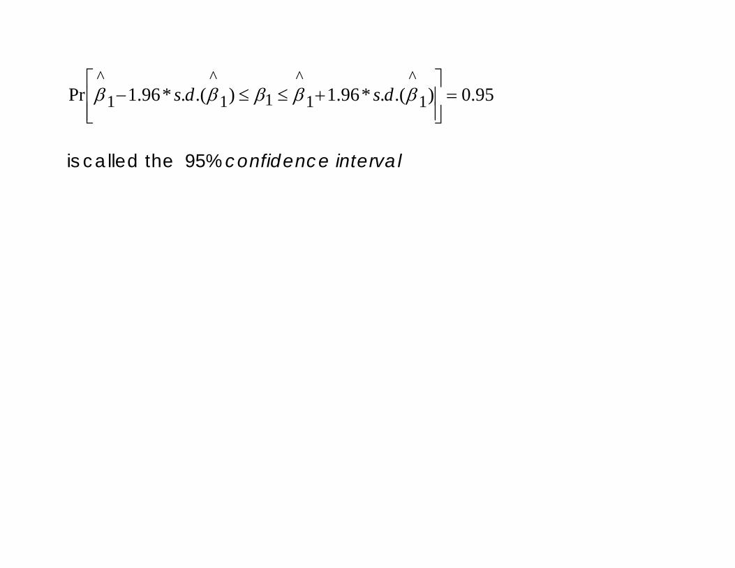
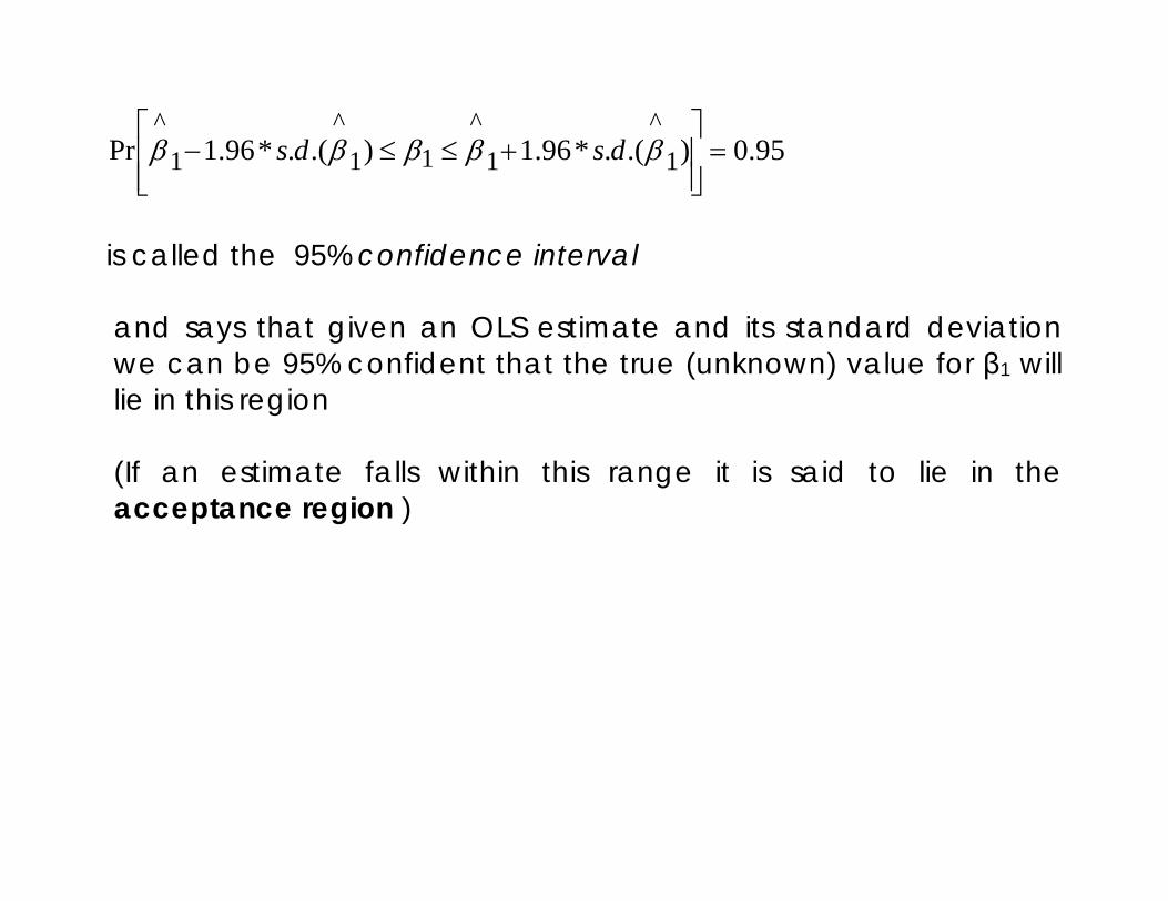
is called the 95% confidence interval

95.0).(.*96.1).(.*96.1Pr 1^
1^
11^
1^
=
+≤≤− βββββ dsds
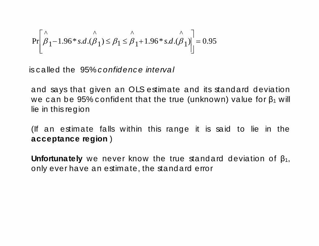
is called the 95% confidence interval and says that given an OLS estimate and its standard deviation we can be 95% confident that the true (unknown) value for β1 will lie in this region
95.0).(.*96.1).(.*96.1Pr 1^
1^
11^
1^
=
+≤≤− βββββ dsds
is called the 95% confidence interval and says that given an OLS estimate and its standard deviation we can be 95% confident that the true (unknown) value for β1 will lie in this region (If an estimate falls within this range it is said to lie in the acceptance region )
95.0).(.*96.1).(.*96.1Pr 1^
1^
11^
1^
=
+≤≤− βββββ dsds
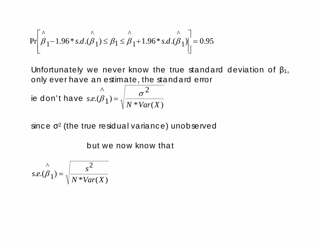
is called the 95% confidence interval and says that given an OLS estimate and its standard deviation we can be 95% confident that the true (unknown) value for β1 will lie in this region (If an estimate falls within this range it is said to lie in the acceptance region ) Unfortunately we never know the true standard deviation of β1, only ever have an estimate, the standard error
95.0).(.*96.1).(.*96.1Pr 1^
1^
11^
1^
=
+≤≤− βββββ dsds
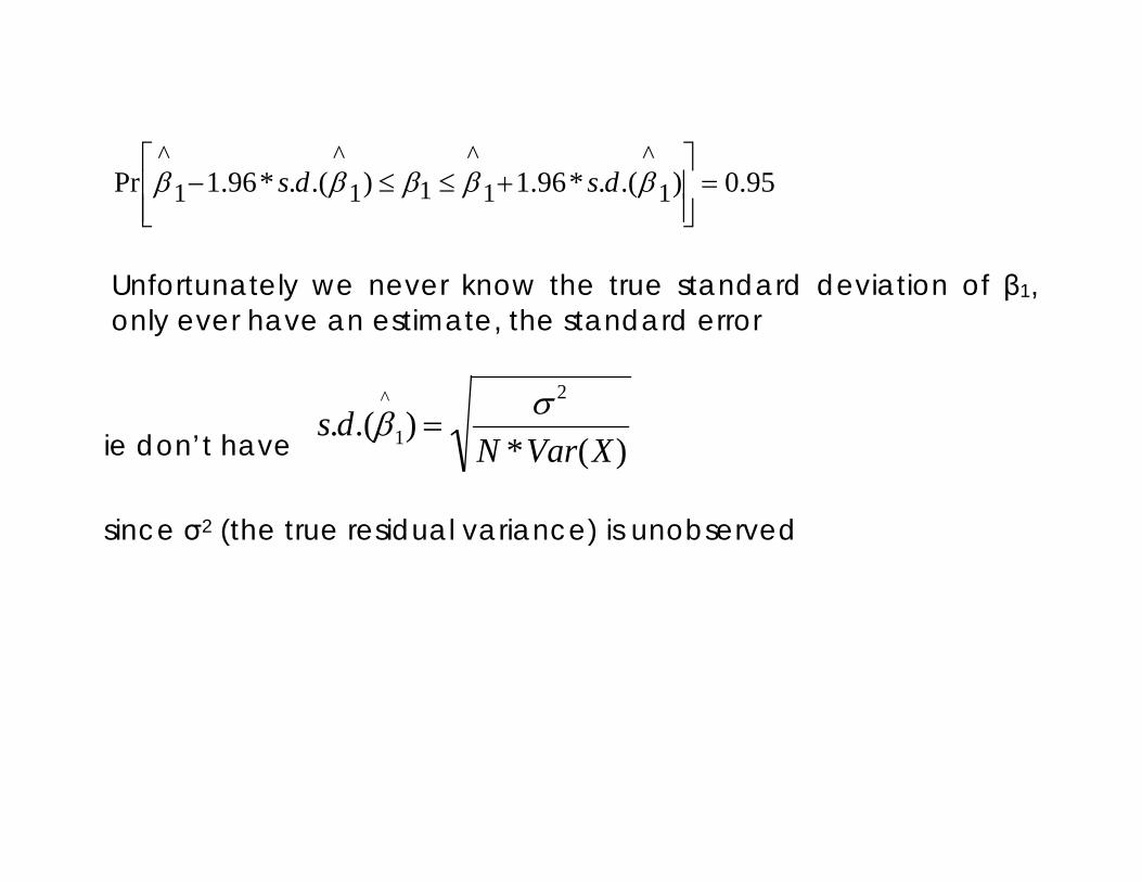
Unfortunately we never know the true standard deviation of β1, only ever have an estimate, the standard error
ie don’t have
s.d.(β^
1) =σ 2
N *Var(X)
since σ2 (the true residual variance) is unobserved
95.0).(.*96.1).(.*96.1Pr 1^
1^
11^
1^
=
+≤≤− βββββ dsds
Unfortunately we never know the true standard deviation of β1, only ever have an estimate, the standard error
ie don’t have )(*
2)1
^.(.
XVarNes σβ =
since σ2 (the true residual variance) unobserved
but we now know that
)(*).(.
21
^
XVarNses =β
95.0).(.*96.1).(.*96.1Pr 1^
1^
11^
1^
=
+≤≤− βββββ dsds
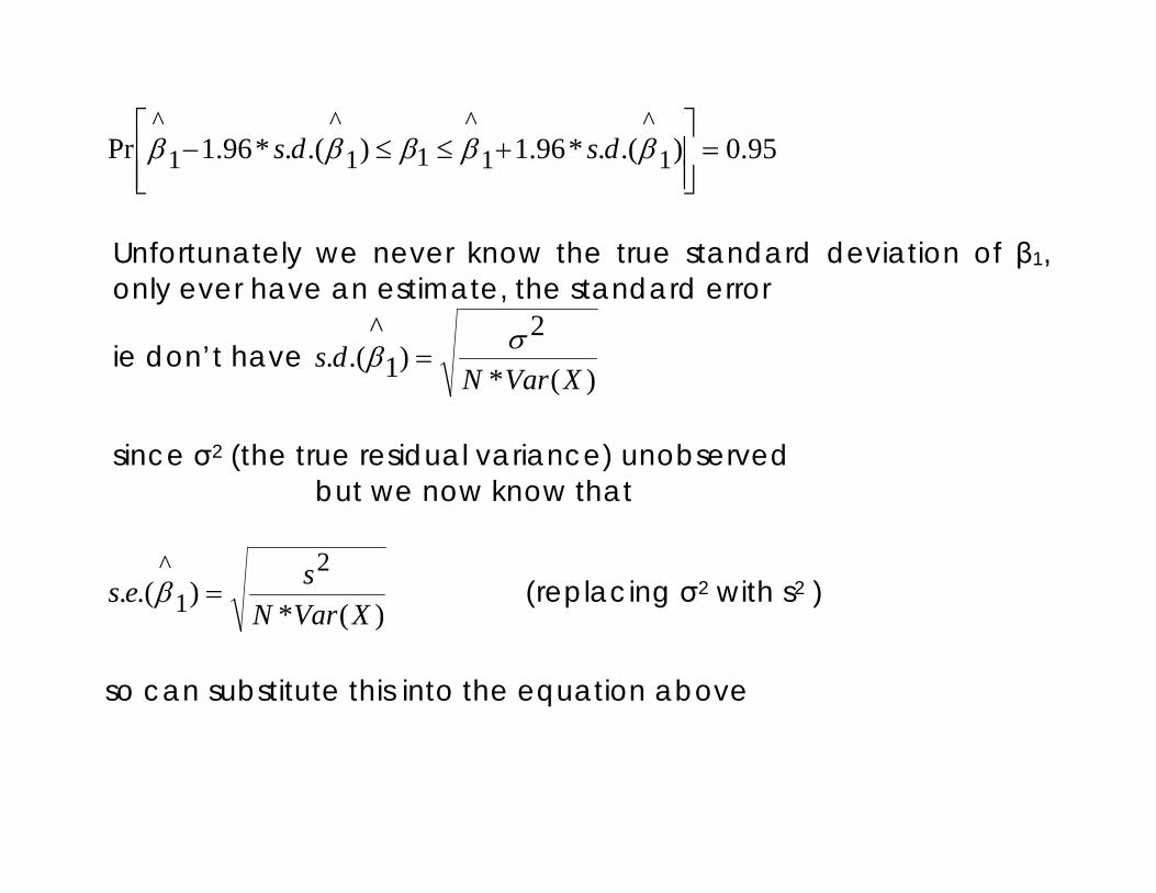
Unfortunately we never know the true standard deviation of β1, only ever have an estimate, the standard error
ie don’t have )(*
2)1
^.(.
XVarNds σβ =
since σ2 (the true residual variance) unobserved
but we now know that
)(*).(.
21
^
XVarNses =β (replacing σ2 with s2 )
so can substitute this into the equation above
95.0).(.*96.1).(.*96.1Pr 1^
1^
11^
1^
=
+≤≤− βββββ dsds
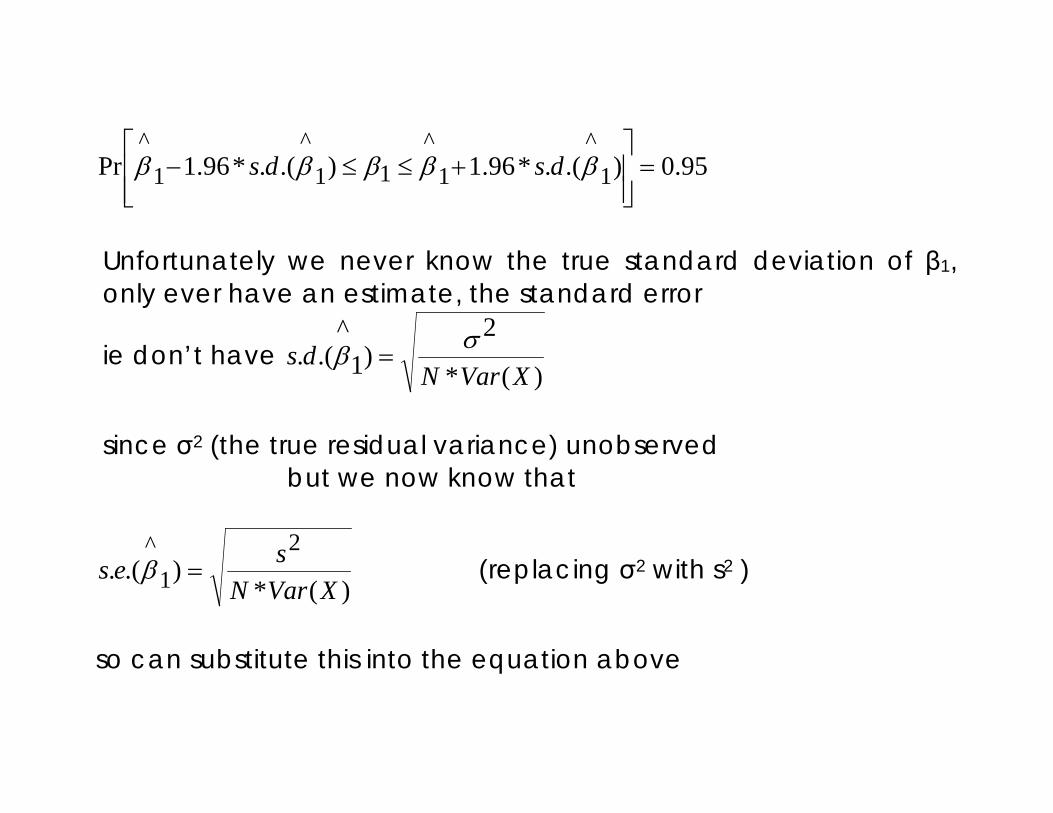
Unfortunately we never know the true standard deviation of β1, only ever have an estimate, the standard error
ie don’t have )(*
2)1
^.(.
XVarNds σβ =
since σ2 (the true residual variance) unobserved
but we now know that
)(*).(.
21
^
XVarNses =β (replacing σ2 with s2 )
so can substitute this into the equation above
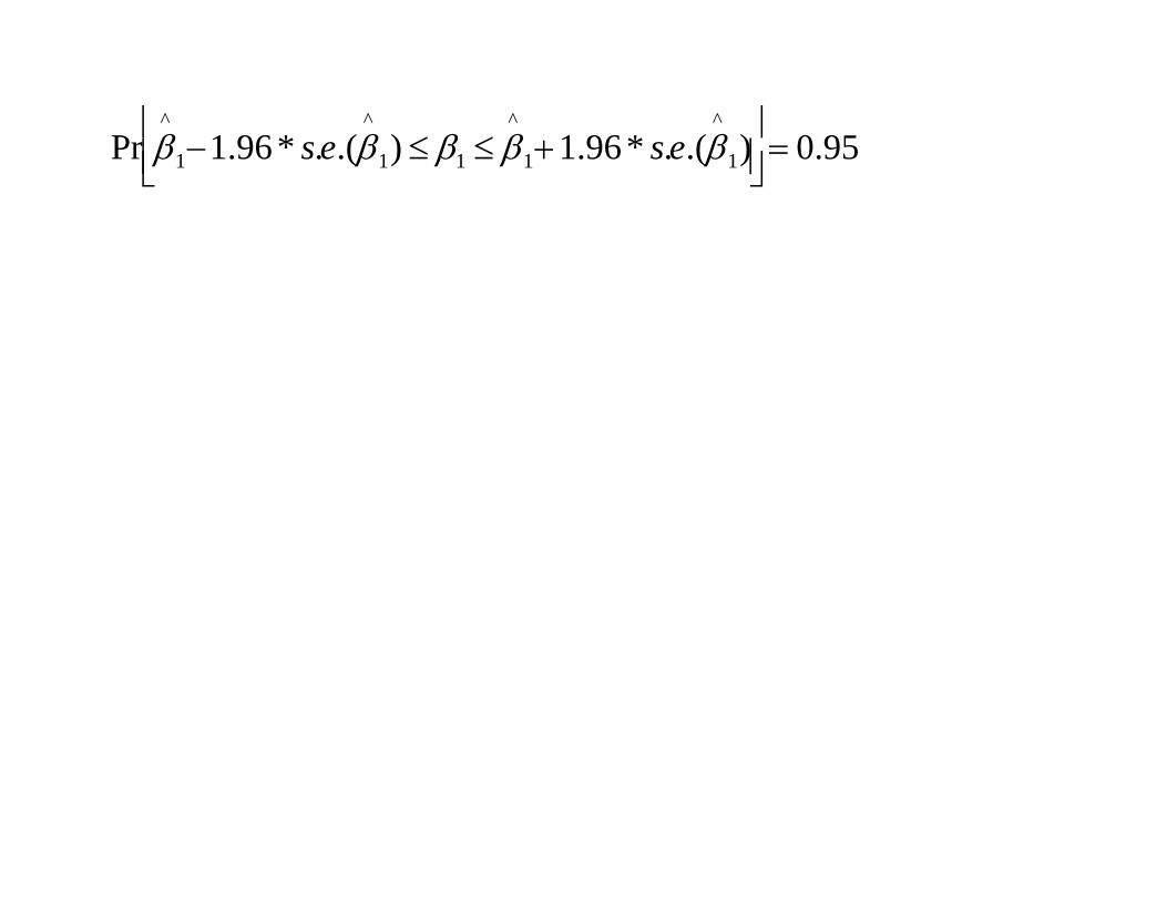
Pr β^
1−1.96 * s.e.(β^
1) ≤ β1 ≤ β^
1+1.96* s.e.(β^
1)
= 0.95

However when we do this we no longer have a standard normal distribution
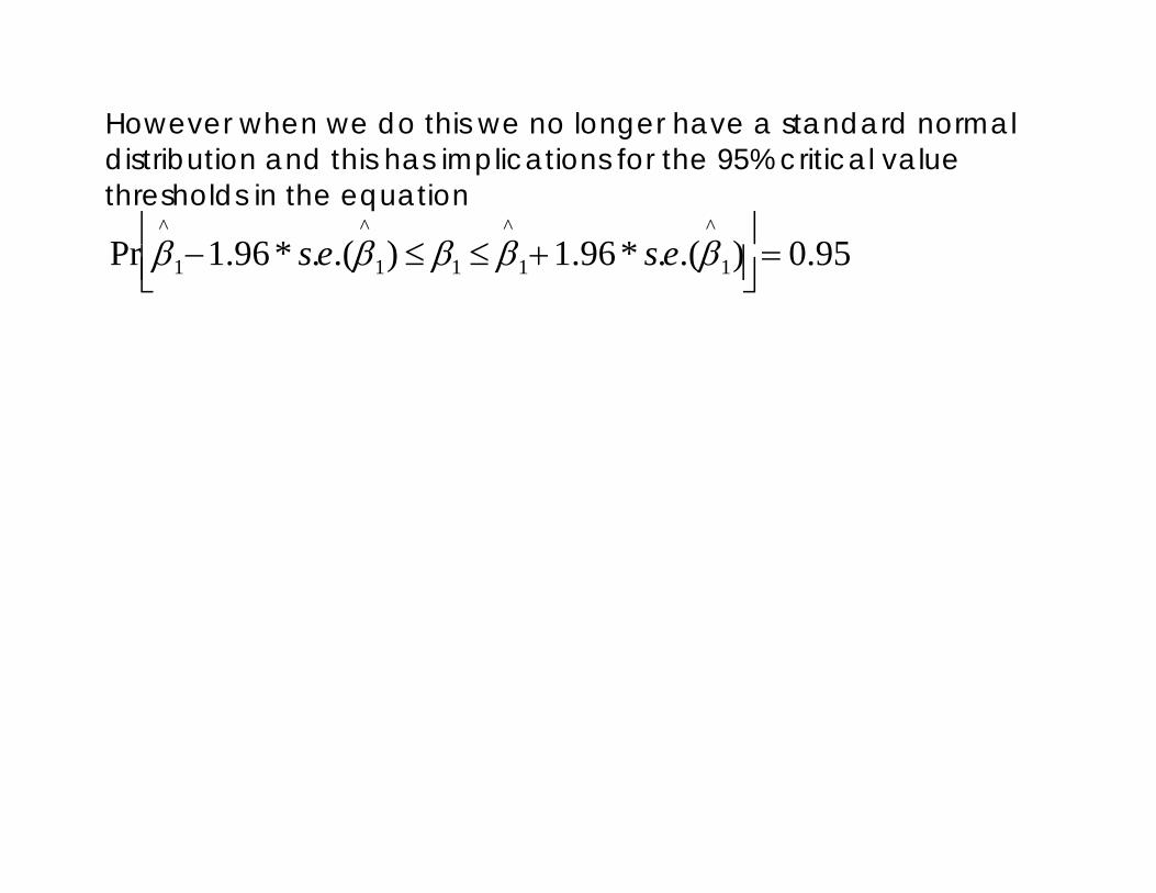
However when we do this we no longer have a standard normal distribution and this has implications for the 95% critical value thresholds in the equation
Pr β^
1−1.96 * s.e.(β^
1) ≤ β1 ≤ β^
1+1.96* s.e.(β^
1)
= 0.95
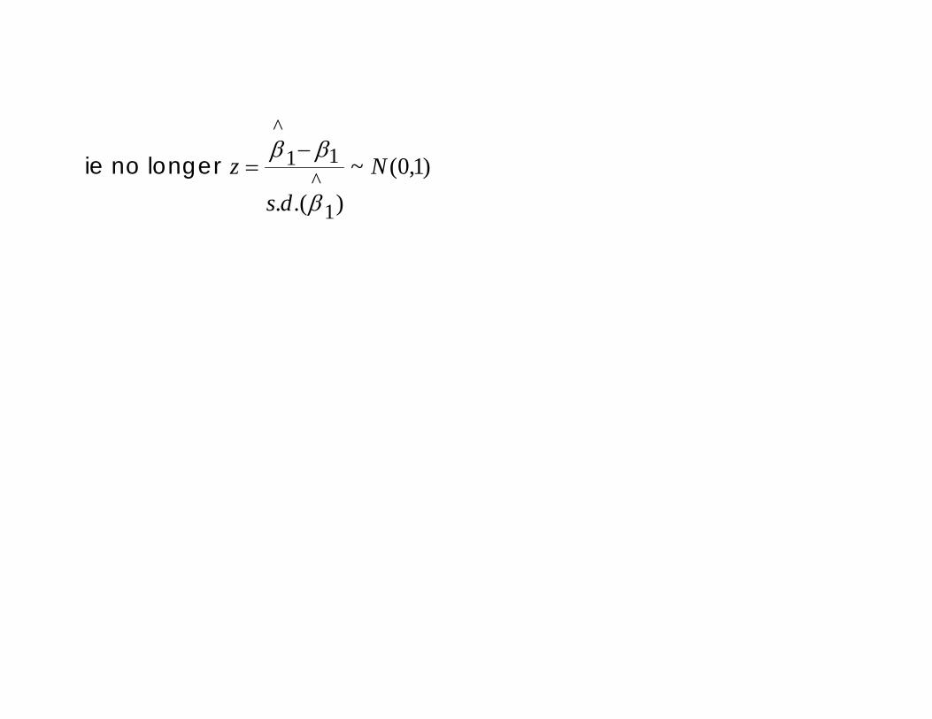
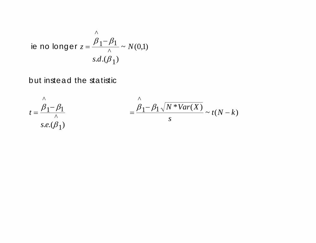
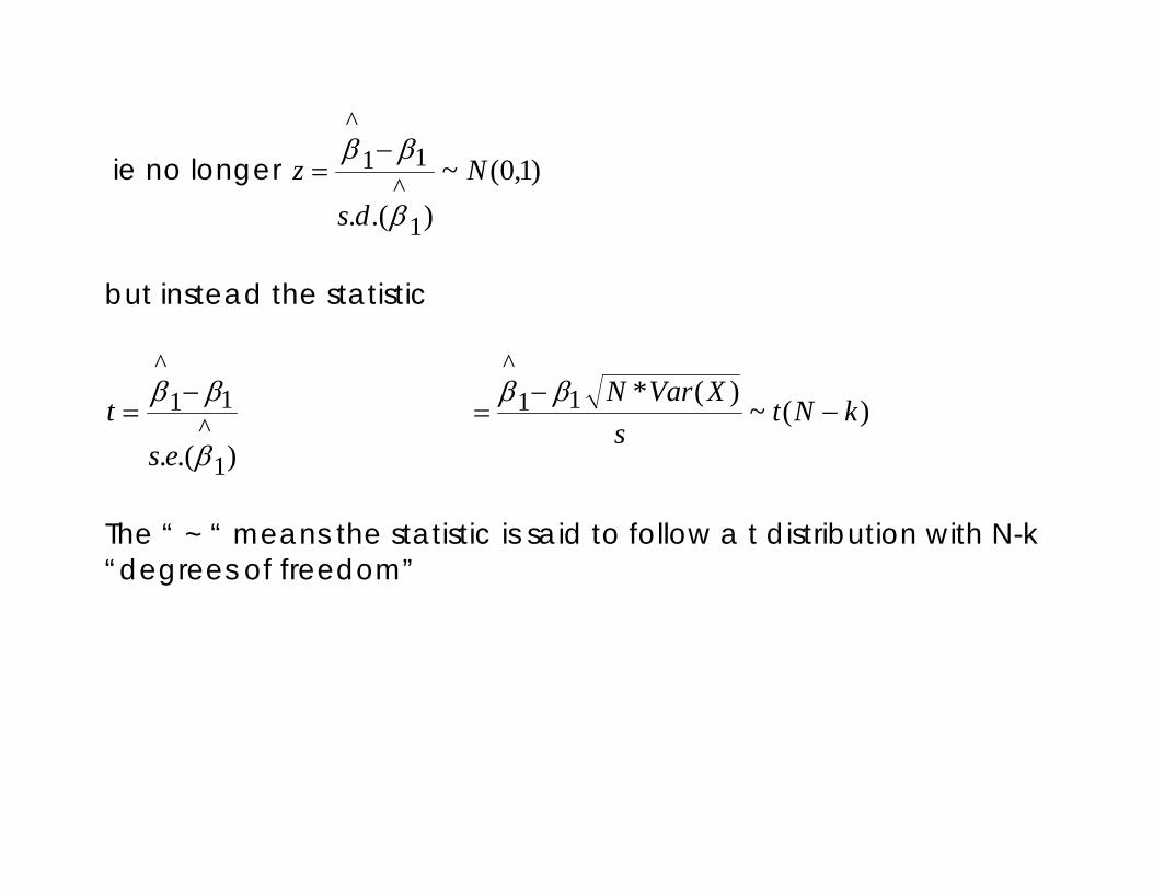
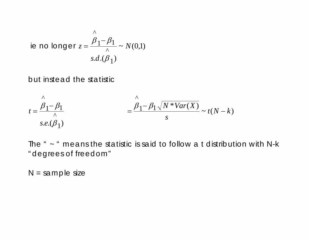
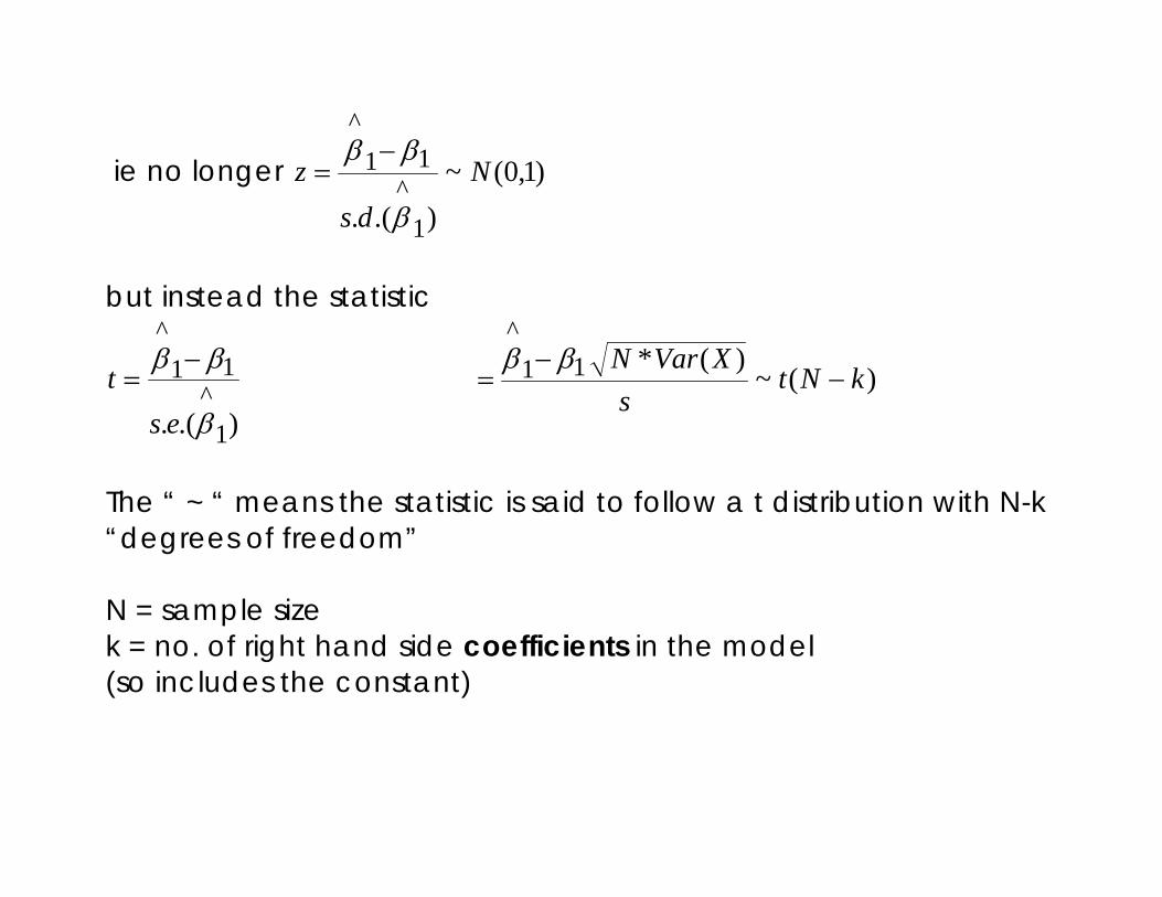
ie no longer )1,0(~).(. 1
^11
^
Nds
zβ
ββ −=
ie no longer )1,0(~).(. 1
^11
^
Nds
zβ
ββ −=
but instead the statistic
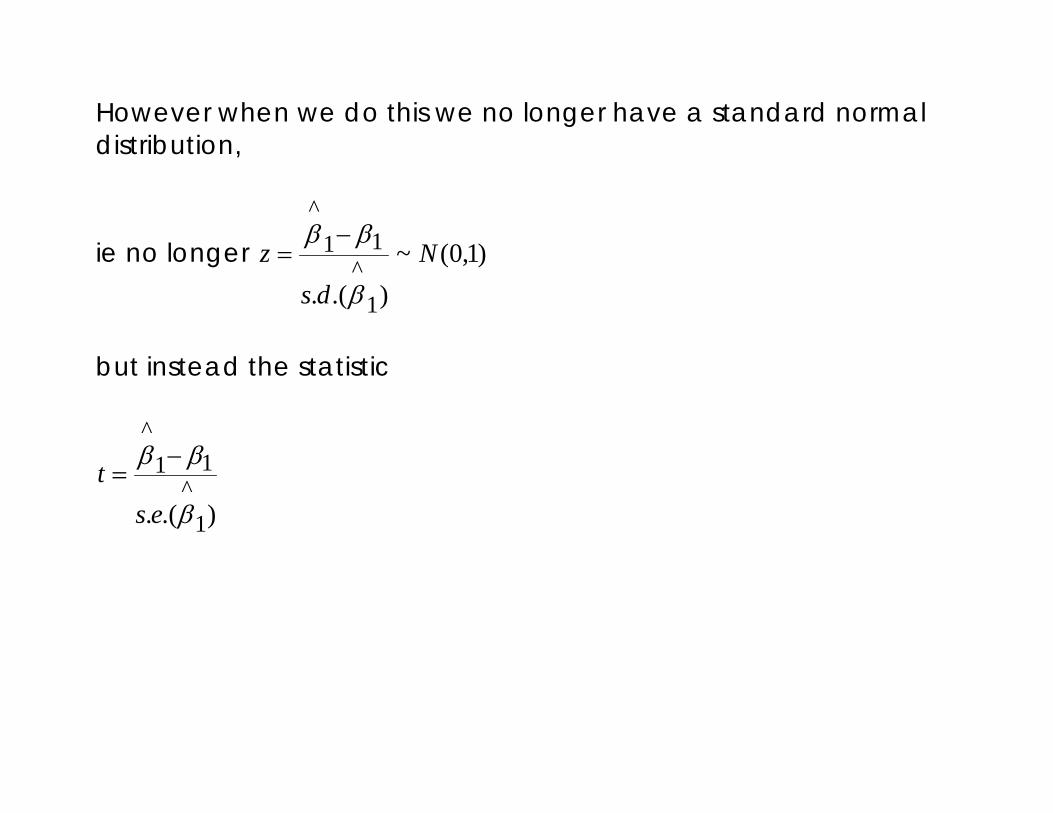
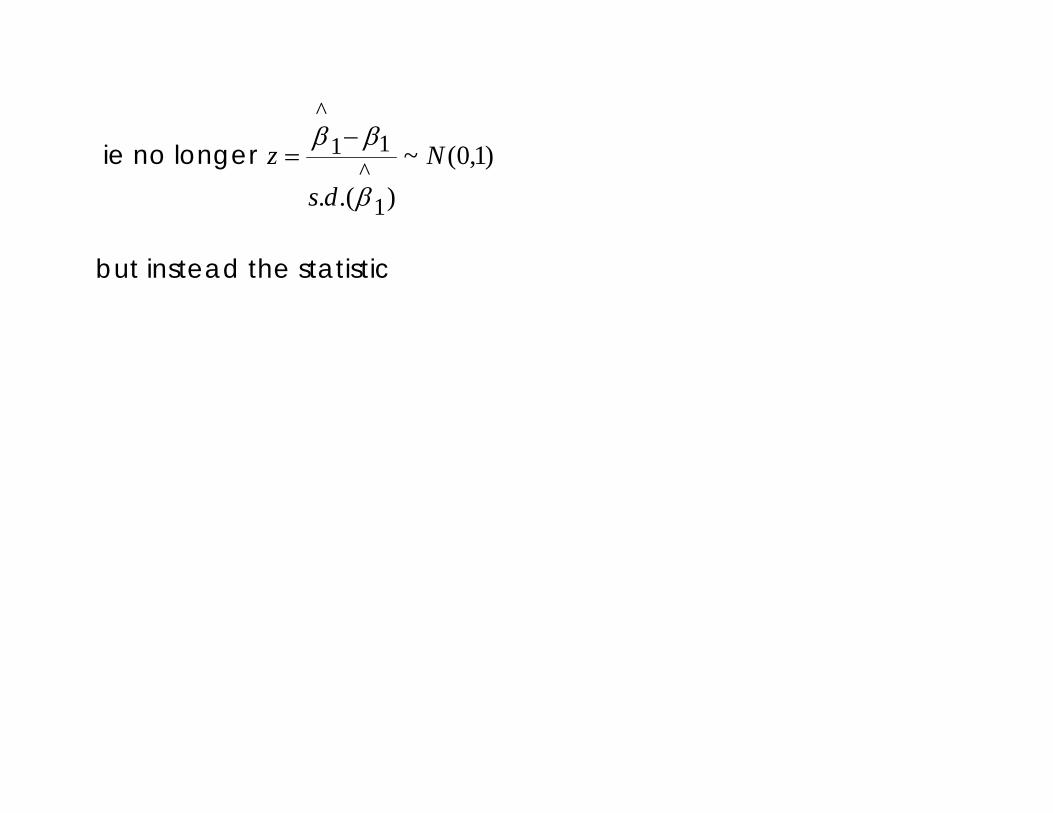
However when we do this we no longer have a standard normal distribution,
ie no longer )1,0(~).(. 1
^11
^
Nds
zβ
ββ −=
but instead the statistic
).(. 1^
11^
β
ββ
est
−=
ie no longer )1,0(~).(. 1
^11
^
Nds
zβ
ββ −=
but instead the statistic
).(. 1^
11^
β
ββ
est
−= )(~
)(*11^
kNts
XVarN−
−=
ββ
ie no longer )1,0(~).(. 1
^11
^
Nds
zβ
ββ −=
but instead the statistic
).(. 1^
11^
β
ββ
est
−= )(~
)(*11^
kNts
XVarN−
−=
ββ
The “ ~ “ means the statistic is said to follow a t distribution with N-k “degrees of freedom”
ie no longer )1,0(~).(. 1
^11
^
Nds
zβ
ββ −=
but instead the statistic
).(. 1^
11^
β
ββ
est
−= )(~
)(*11^
kNts
XVarN−
−=
ββ
The “ ~ “ means the statistic is said to follow a t distribution with N-k “degrees of freedom” N = sample size
ie no longer )1,0(~).(. 1
^11
^
Nds
zβ
ββ −=
but instead the statistic
).(. 1^
11^
β
ββ
est
−= )(~
)(*11^
kNts
XVarN−
−=
ββ
The “ ~ “ means the statistic is said to follow a t distribution with N-k “degrees of freedom” N = sample size k = no. of right hand side coefficients in the model (so includes the constant)

Student’s t distribution introduced by William Gosset 1976-1937 and developed by Ronald Fisher 1890-1962
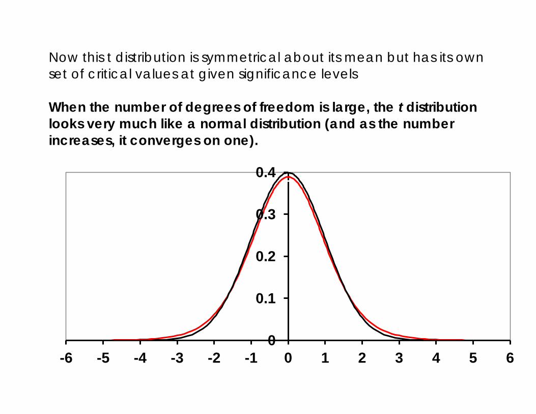
Now this t distribution is symmetrical about its mean but has its own set of critical values at given significance levels When the number of degrees of freedom is large, the t distribution looks very much like a normal distribution (and as the number increases, it converges on one).
0
0.1
0.2
0.3
0.4
-6 -5 -4 -3 -2 -1 0 1 2 3 4 5 6
Now this t distribution is symmetrical about its mean but has its own set of critical values at given significance levels which vary, unlike the standard normal distribution, with the degrees of freedom in the model,
Now this t distribution is symmetrical about its mean but has its own set of critical values at given significance levels which vary, unlike the standard normal distribution, with the degrees of freedom in the model, N-K
Now this t distribution is symmetrical about its mean but has its own set of critical values at given significance levels which vary, unlike the standard normal distribution, with the degrees of freedom in the model, N-K which means the “degrees of freedom” depend on the sample size and the number of variables in the model)
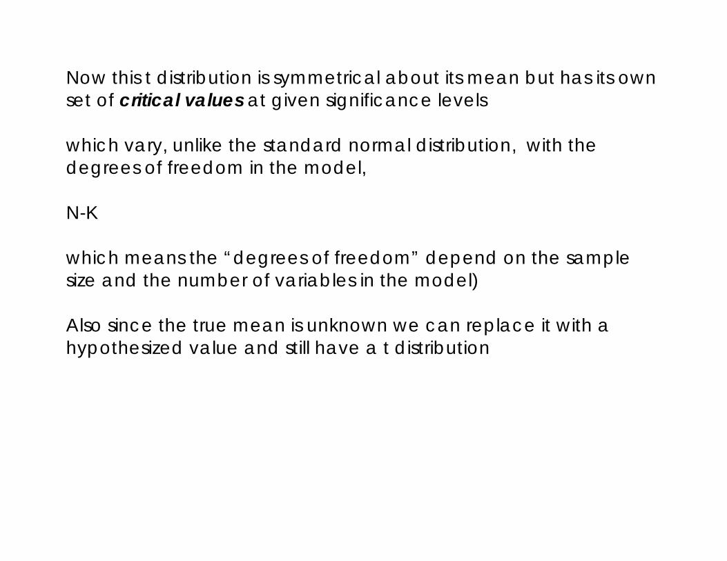
Now this t distribution is symmetrical about its mean but has its own set of critical values at given significance levels which vary, unlike the standard normal distribution, with the degrees of freedom in the model, N-K which means the “degrees of freedom” depend on the sample size and the number of variables in the model) Also since the true mean is unknown we can replace it with a hypothesized value and still have a t distribution
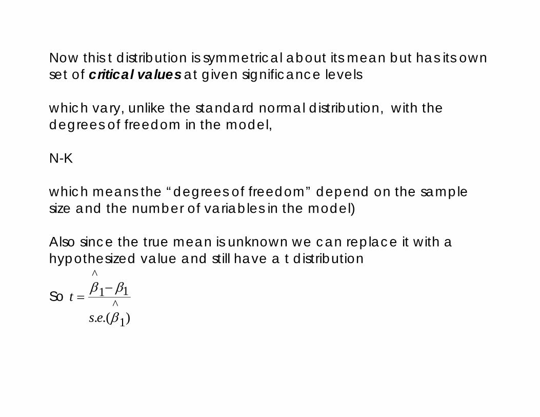
Now this t distribution is symmetrical about its mean but has its own set of critical values at given significance levels which vary, unlike the standard normal distribution, with the degrees of freedom in the model, N-K which means the “degrees of freedom” depend on the sample size and the number of variables in the model) Also since the true mean is unknown we can replace it with a hypothesized value and still have a t distribution
So ).(. 1
^11
^
β
ββ
est
−=
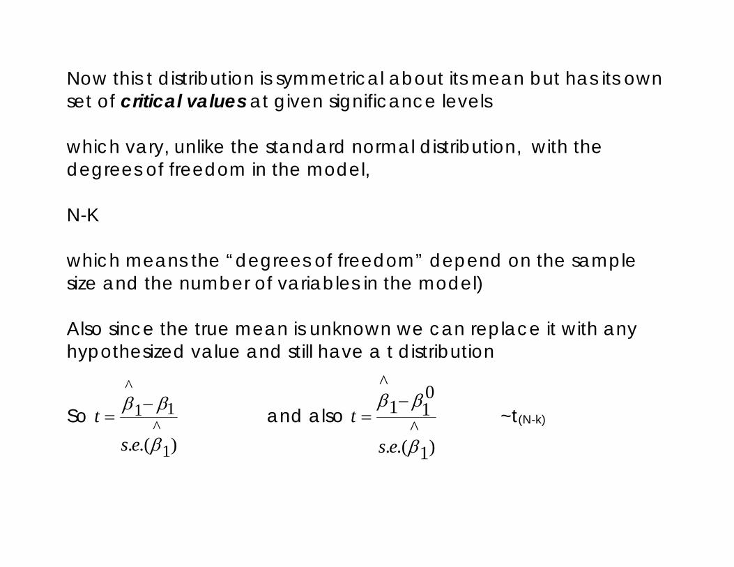
Now this t distribution is symmetrical about its mean but has its own set of critical values at given significance levels which vary, unlike the standard normal distribution, with the degrees of freedom in the model, N-K which means the “degrees of freedom” depend on the sample size and the number of variables in the model) Also since the true mean is unknown we can replace it with any hypothesized value and still have a t distribution
So ).(. 1
^11
^
β
ββ
est
−= and also
)1^
.(.
011
^
β
ββ
est
−= ~t(N-k)

Related Documents