Lecture 4. The parabolic equations and time dependent Stokes problem Ching-hsiao (Arthur) Cheng Department of Mathematics National Central University Taiwan, ROC The National Center for Theoretic Sciences, Summer 2012 Ching-hsiao Cheng Lecture 4. The parabolic theory and Stokes equations

Welcome message from author
This document is posted to help you gain knowledge. Please leave a comment to let me know what you think about it! Share it to your friends and learn new things together.
Transcript

Lecture 4. The parabolic equations and timedependent Stokes problem
Ching-hsiao (Arthur) Cheng
Department of MathematicsNational Central University
Taiwan, ROC
The National Center for Theoretic Sciences, Summer 2012
Ching-hsiao Cheng Lecture 4. The parabolic theory and Stokes equations

Parabolic equations
Let Ω ⊆ Rn be a bounded and smooth domain. We consider
ut + Lu = f in Ω× (0,T ),
u = u0 on Ω× t = 0,boundary conditions on ∂Ω× (0,T ),
where Lu is a (time-dependent) uniformly elliptic operator
defined byLu = − ∂
∂xi
(aij ∂u∂xj
)+ bi ∂u
∂xi+ cu.
Here the coefficients a, b, c may depend on t . We recall that L
is called uniformly elliptic if there exists constant λ > 0 such that
aijξiξj ≥ λ|ξ|2 ∀ ξ ∈ Rn.
∂t + L is called uniformly parabolic if L is uniformly elliptic.
Ching-hsiao Cheng Lecture 4. The parabolic theory and Stokes equations

Boundary conditions
Two types of boundary conditions are considered.
1 Dirichlet boundary condition:
u = 0 on ∂Ω× (0,T ).
2 Neumann boundary condition:
aij ∂u∂xj
Ni = g on ∂Ω× (0,T ).
A Robin type of boundary condition can also be considered, but
the theory behind that is similar to the Neumann problem, so
we ignore the discussion of such boundary condition.
Ching-hsiao Cheng Lecture 4. The parabolic theory and Stokes equations
The parabolic equations
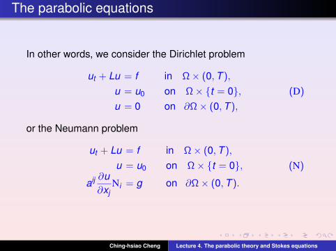
In other words, we consider the Dirichlet problem
ut + Lu = f in Ω× (0,T ),
u = u0 on Ω× t = 0, (D)
u = 0 on ∂Ω× (0,T ),
or the Neumann problem
ut + Lu = f in Ω× (0,T ),
u = u0 on Ω× t = 0, (N)
aij ∂u∂xj
Ni = g on ∂Ω× (0,T ).
Ching-hsiao Cheng Lecture 4. The parabolic theory and Stokes equations

The weak formulation and weak solutions
Assume that aij ,bi , c ∈ L∞(Ω× (0,T )), f ∈ L2(0,T ; L2(Ω)),
and u0 ∈ L2(Ω).
Definition (Weak solutions with Dirichlet boundary conditions)
A function u ∈ L2(0,T ; H10 (Ω)) with ut ∈ L2(0,T ; H−1(Ω)) is
said to be a weak solution of (D) provided that
〈ut , ϕ〉+ B(u, ϕ) =(f , ϕ)
L2(Ω)∀ϕ ∈ H1
0 (Ω), a.e. t ∈ (0,T ),
andu(0) = u0 ,
where B(u, ϕ) is defined by
B(u, ϕ) ≡∫
Ω
[aij ∂u∂xj
∂ϕ
∂xi+ bi ∂u
∂xiϕ+ cuϕ
]dx .
The integral equality is called the variational formulation of (D).
Ching-hsiao Cheng Lecture 4. The parabolic theory and Stokes equations

The weak formulation and weak solutions
Assume further that g ∈ L2(0,T ; L2(∂Ω)).
Definition (Weak solutions with Neumann boundary conditions)
A function u ∈ L2(0,T ; H1(Ω)) with ut ∈ L2(0,T ; H1(Ω)′) is saidto be a weak solution of (D) provided that
〈ut , ϕ〉+ B(u, ϕ) = (f , ϕ)L2(Ω) + (g, ϕ)L2(∂Ω)
∀ϕ ∈ H1(Ω), a.e. t ∈ (0,T ),
andu(0) = u0 ,
where B(u, ϕ) is defined by
B(u, ϕ) ≡∫
Ω
[aij ∂u∂xj
∂ϕ
∂xi+ bi ∂u
∂xiϕ+ cuϕ
]dx .
The integral equality is called the variational formulation of (N).
Ching-hsiao Cheng Lecture 4. The parabolic theory and Stokes equations

The meaning of u(0) = u0
For H = H10 (Ω;Rn) or H = H1(Ω), the initial value of a function
u ∈ L2(0,T ;H) does not make sense. However, since ut is
required to belong to L2(0,T ;H ′) in the definition of the weak
solution, the following “time embedding lemma”
Lemma
Suppose u ∈ L2(0,T ;H), with ut ∈ L2(0,T ;H ′) for some Hilbertspace H so that H →L2(Ω) ⊆ H ′. Then u ∈ C([0,T ]; L2(Ω)),and
maxt∈[0,T ]
‖u(t)‖L2(Ω) ≤(
1 +1T
)[‖u‖L2(0,T ;H) + ‖ut‖L2(0,T ;H ′)
].
suggests that u ∈ C([0,T ]; L2(Ω)); thus u(0) makes sense, and
limt→0+
‖u(t)− u0‖L2(Ω) = 0.
Ching-hsiao Cheng Lecture 4. The parabolic theory and Stokes equations

The existence and uniqueness of the weak solution
Note that the general form of the weak formulation above is
〈ut , ϕ〉+ (∇u,∇ϕ)L2(Ω) = F (ϕ) ∀ϕ ∈ H, a.e. t ∈ (0,T ).
Construction of a weak solution - the Galerkin method: Let
ek∞k=1 be an orthogonal basis in H which is orthogonal in Hand orthonormal in L2(Ω). For each k ∈ N, let
uk (x , t) =k∑
`=1
dk` (t)e`(x)
satisfy
(ukt (t), ϕ)L2(Ω) + B(uk (t), ϕ
)= F (ϕ) ∀ ϕ ∈ span(e1, · · · , ek ).
and
dk` (0) = (u0, e`)L2(Ω) ∀ 1 ≤ ` ≤ k .
Ching-hsiao Cheng Lecture 4. The parabolic theory and Stokes equations
The existence and uniqueness of the weak solution
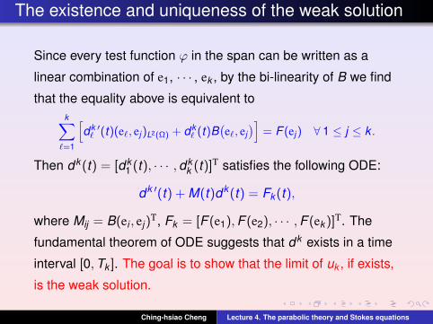
Since every test function ϕ in the span can be written as a
linear combination of e1, · · · , ek , by the bi-linearity of B we find
that the equality above is equivalent tok∑
`=1
[dk ′` (t)(e`, ej )L2(Ω) + dk
` (t)B(e`, ej
)]= F (ej ) ∀ 1 ≤ j ≤ k .
Then dk (t) = [dk1 (t), · · · ,dk
k (t)]T satisfies the following ODE:
dk ′(t) + M(t)dk (t) = Fk (t),
where Mij = B(ei , ej)T, Fk = [F (e1),F (e2), · · · ,F (ek )]T. The
fundamental theorem of ODE suggests that dk exists in a time
interval [0,Tk ]. The goal is to show that the limit of uk , if exists,
is the weak solution.
Ching-hsiao Cheng Lecture 4. The parabolic theory and Stokes equations

The existence and uniqueness of the weak solution
Question 1: Is there a positive lower bound of Tk? If not, the
limit of uk means nothing.
Question 2: How do we ensure that uk converges? If uk does
converge, in what space and in what sense?
Answer: We need to look at the so-called energy estimates.
The starting point is that uk satisfies(ukt (t), ej
)L2(Ω)
+ B(uk (t), ej
)= F (ej ) ∀ 1 ≤ j ≤ k ;
thus by the bi-linearity of B and linearity of F ,(ukt (t),uk (t)
)L2(Ω)
+ B(uk (t),uk (t)
)= F
(uk (t)
)⇒ 1
2ddt‖uk (t)‖2
L2(Ω) + B(uk (t),uk (t)
)= F
(uk (t)
)
Ching-hsiao Cheng Lecture 4. The parabolic theory and Stokes equations
The existence and uniqueness of the weak solution
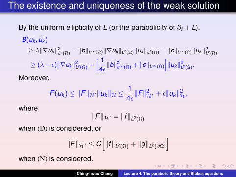
By the uniform ellipticity of L (or the parabolicity of ∂t + L),
B(uk ,uk )
≥ λ‖∇uk‖2L2(Ω) − ‖b‖L∞(Ω)‖∇uk‖L2(Ω)‖uk‖L2(Ω) − ‖c‖L∞(Ω)‖uk‖2
L2(Ω)
≥ (λ− ε)‖∇uk‖2L2(Ω) −
[ 14ε‖b‖2
L∞(Ω) + ‖c‖L∞(Ω)
]‖uk‖2
L2(Ω).
Moreover,
F (uk ) ≤ ‖F‖H ′‖uk‖H ≤14ε‖F‖2H ′ + ε‖uk‖2H,
where‖F‖H ′ = ‖f‖L2(Ω)
when (D) is considered, or
‖F‖H ′ ≤ C[‖f‖L2(Ω) + ‖g‖L2(∂Ω)
]when (N) is considered.
Ching-hsiao Cheng Lecture 4. The parabolic theory and Stokes equations

The existence and uniqueness of the weak solution
Therefore, letting ε = λ/4, we find that
12
ddt‖uk (t)‖2
L2(Ω) +λ
2‖∇uk (t)‖2
L2(Ω) ≤λ
4‖uk (t)‖2
L2(Ω) +1λ‖F (t)‖2
H ′ .
Integrating the inequality in time over the time interval (0, t), we
obtain that
‖uk (t)‖2L2(Ω) + λ
∫ t
0‖∇uk (s)‖2
L2(Ω)ds
≤ ‖uk (0)‖2L2(Ω) +
2λ‖F‖2
L2(0,T ;H ′)) +λ
2
∫ t
0‖uk (s)‖2
L2(Ω)ds
≤ ‖u0‖2L2(Ω) +
2λ‖F‖2
L2(0,T ;H ′)︸ ︷︷ ︸≡M
+λ
2
∫ t
0‖uk (s)‖2
L2(Ω)ds.
Ching-hsiao Cheng Lecture 4. The parabolic theory and Stokes equations
The existence and uniqueness of the weak solution
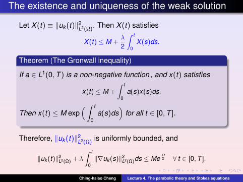
Let X (t) ≡ ‖uk (t)‖2L2(Ω). Then X (t) satisfies
X (t) ≤ M +λ
2
∫ t
0X (s)ds.
Theorem (The Gronwall inequality)
If a ∈ L1(0,T ) is a non-negative function , and x(t) satisfies
x(t) ≤ M +
∫ t
0a(s)x(s)ds.
Then x(t) ≤ M exp(∫ t
0a(s)ds
)for all t ∈ [0,T ].
Therefore, ‖uk (t)‖2L2(Ω)is uniformly bounded, and
‖uk (t)‖2L2(Ω) + λ
∫ t
0‖∇uk (s)‖2
L2(Ω)ds ≤ Meλt2 ∀ t ∈ [0,T ].
Ching-hsiao Cheng Lecture 4. The parabolic theory and Stokes equations

The existence and uniqueness of the weak solution
Implications:
1 ‖uk (t)‖2L2(Ω) =
k∑=1|dk
` (t)|2 is bounded uniformly in k ; thus
Tk ≥ T for some fixed T > 0.
2 For ϕ ∈ H, write ϕ = ϕ1 + ϕ2 with ϕ1 ∈ span(e1, · · · , ek )
and ϕ2 ⊥ ϕ1. By the definition of the dual space norm,
‖ukt‖H ′ = sup‖ϕ‖H=1
〈ukt , ϕ〉 = sup‖ϕ‖H=1
(ukt , ϕ1)L2(Ω)
= sup‖ϕ‖H=1
[F (ϕ1)− B(uk , ϕ1)
]≤ C
[‖F‖H ′ + ‖uk‖H
].
Since uk is bounded in L2(0,T ;H) uniformly in k , ukt is
uniformly bounded in L2(0,T ;H ′).
Ching-hsiao Cheng Lecture 4. The parabolic theory and Stokes equations

The existence and uniqueness of the weak solution
3 Since L2(0,T ;H) and L2(0,T ;H ′) are both Hilbert spaces,
by Banach-Alouglu theorem, there exists a subsequence
ukj of uk such that ukj and ukj t converge weakly in
L2(0,T ;H) and L2(0,T ;H ′), respectively.
4 ukj satisfies
(ukj t , v)L2(Ω) + B(ukj , v) = F (v)
∀ v =k∑
`=1
d`(t)e`(x), a.e. t ∈ (0,T );
thus passing j to the limit, we conclude that∫ T
0
[⟨ut (t), v(t)
⟩+ B
(u(t), v(t)
)]dt =
∫ T
0F(v(t)
)dt
∀ v ∈ L2(0,T ;H).
Ching-hsiao Cheng Lecture 4. The parabolic theory and Stokes equations

The existence and uniqueness of the weak solution
5 The use of v(x , t) = χ(a,b)(t)ϕ(x) for some 0 ≤ a < b ≤ T
implies that∫ b
a
[⟨ut (t), ϕ
⟩+ B
(u(t), ϕ
)]dt =
∫ b
aF(ϕ)dt ∀ ϕ ∈ H.
Therefore, the Lebesgue differentiation theorem
suggests that u satisfies the variational formulation.
Question: u(0) = u0? This is the same as asking that if
limt→0
limj→∞
ukj (t) = limj→∞
limt→0
ukj (t),
where the limit as j →∞ is taken in the sense of L2, and the
limit as t → 0 is taken in the sense of C0.
Ching-hsiao Cheng Lecture 4. The parabolic theory and Stokes equations

The existence and uniqueness of the weak solution
Answer: Let ζ ∈ C1([0,T ]) such that ζ(0) = 1 and ζ(T ) = 0.
Then∫ T
0
[(ukj t (t), ζ(t)ϕ
)L2(Ω)
+ B(ukj (t), ζ(t)ϕ
)]dt =
∫ T
0F(ζ(t)ϕ
)dt
∀ ϕ ∈ span(e1, · · · , ekj ),
and ∫ T
0
[⟨ut (t), ζ(t)ϕ
⟩+ B
(u(t), ζ(t)ϕ
)]dt =
∫ T
0F(v(t)
)dt
∀ ϕ ∈ H.
Integrating by parts in time for the first term and then passing j
to the limit, we find that
limj→∞
(ukj (0), ϕ
)L2(Ω)
=(u(0), ϕ
)L2(Ω)
∀ϕ ∈ H
which implies that u(0) = u0; thus u is a weak solution.
Ching-hsiao Cheng Lecture 4. The parabolic theory and Stokes equations

The existence and uniqueness of the weak solution
Uniqueness: Suppose that u1 and u2 are two weak solutions.
Let u = u1 − u2. Then u ∈ L2(0,T ;H) with ut ∈ L2(0,T ;H ′)satisfies∫ T
0
[〈ut (t), v(t)〉+ B
(u(t), v(t)
)]dt = 0 ∀ v ∈ L2(0,T ;H)
andu(0) = 0.
Let v(t) = χ(0,s)u(t) be a test function, we conclude that
‖u(s)‖2L2(Ω) + λ‖∇u(s)‖2
L2(Ω) ≤λ
2
∫ s
0‖u(t)‖2
L2(Ω)dt ;
thus the Gronwall inequality implies that ‖u(t)‖L2(Ω) = 0 for all
t ∈ [0,T ]. This suggests that the weak solution is unique.
Ching-hsiao Cheng Lecture 4. The parabolic theory and Stokes equations

The existence and uniqueness of the weak solution
Some remarks:
1 Unlike the case of elliptic equations, even if b or c is not
identical to zero, the weak solution always exists. This is
because the L2-norm of u is controlled by the ut term.
2 The estimates we derive for uk in L∞(0,T ; L2(Ω)) and
L2(0,T ;H) can also be done formally by testing the
equation against u (and so on). The estimates obtained in
this way are called a priori estimates which will suggest
what the solution space should be.
3 Almost all the a priori estimates can be derives rigorously,
so later on we only try to obtain the estimates formally.
Ching-hsiao Cheng Lecture 4. The parabolic theory and Stokes equations

The regularity theory of parabolic equations
The regularity theory of parabolic equations is based on elliptic
regularity in the following sense: to improve the regularity of u,
we first try to get better regularity of ut and then convert the
equation toLu = f − ut in Ω,
and use elliptic regularity to obtain better regularity of u.
Ching-hsiao Cheng Lecture 4. The parabolic theory and Stokes equations
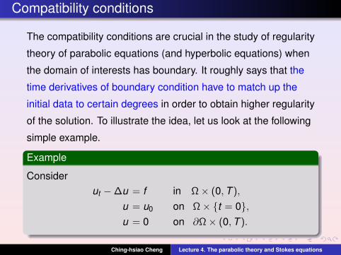
Compatibility conditions
The compatibility conditions are crucial in the study of regularity
theory of parabolic equations (and hyperbolic equations) when
the domain of interests has boundary. It roughly says that the
time derivatives of boundary condition have to match up the
initial data to certain degrees in order to obtain higher regularity
of the solution. To illustrate the idea, let us look at the following
simple example.
Example
Considerut −∆u = f in Ω× (0,T ),
u = u0 on Ω× t = 0,u = 0 on ∂Ω× (0,T ).
Ching-hsiao Cheng Lecture 4. The parabolic theory and Stokes equations

Compatibility conditions
Example (Continued...)
Having established the existence of the unique weak solution
u ∈ L2(0,T ; H10 (Ω)) with ut ∈ L2(0,T ; H−1(Ω)), suppose now
u ∈ L2(0,T ; H2(Ω)). Then ut ∈ L2(0,T ; L2(Ω)) which implies
that u ∈ C([0,T ]; H1(Ω)). Therefore, u ∈ C([0,T ]; H1/2(∂Ω))
which suggest that
limt→0‖u − u0‖H1/2(∂Ω) = 0.
Since u = 0 on boundary, the equality above suggests that
u0 = 0 on ∂Ω. This is the first order compatibility condition that
u0 has to satisfy.
Ching-hsiao Cheng Lecture 4. The parabolic theory and Stokes equations

Example (Continued...)
Suppose that we would like to establish u ∈ L2(0,T ; H4(Ω)).
Then ut ∈ L2(0,T ; H2(Ω)) and utt ∈ L2(0,T ; L2(Ω)). The time
embedding lemma implies that u ∈ C([0,T ]; H3(Ω)) and
ut ∈ C([0,T ]; H1(Ω)). Similar to the previous case, that
u ∈ C([0,T ]; H3(Ω)) implies that u0 = 0 on the boundary.
Moreover, ut = f + ∆u in Ω and ut = 0 on ∂Ω, the fact that
ut ∈ C([0,T ]; H1(Ω)) implies that
limt→0‖ut − ut (0)‖H1/2(∂Ω) = 0
which implies the second order compatibility condition
∆u0 = f (0) on ∂Ω.
Ching-hsiao Cheng Lecture 4. The parabolic theory and Stokes equations

Compatibility conditions
Define uk =∂k−1
∂tk−1
∣∣∣t=0
(f − Lu) for k ∈ N.
Definition (Compatibility conditions for (D))
For k ∈ N ∪ 0, the (k + 1)th-order compatibility condition forthe parabolic initial-boundary value problem (D) is given by
uk = 0 on ∂Ω.
Definition (Compatibility conditions for (N))
For k ∈ N ∪ 0, the (k + 1)th-order compatibility condition forthe parabolic initial-boundary value problem (N) is given by
aij (0)∂uk
∂xjNi =
∂k g∂tk (0)− Ni
k−1∑`=0
(k`
)∂k−`aij
∂tk−` (0)∂u`
∂xjon ∂Ω ,
Ching-hsiao Cheng Lecture 4. The parabolic theory and Stokes equations

The functional framework for parabolic equations
We introduce the function spaces that consist of space-time
dependent functions so that one time derivative scales like two
space derivatives. For k ≥ 1, we define
V kD (T ; Ω)
≡
u ∈ L2(0,T ; Hk (Ω))∣∣∣∂ j
t u ∈ L2(0,T ; Hk−2j (Ω)) if 0≤ j≤[
k+12
],
andV k
N (T ; Ω)
≡
u ∈ L2(0,T ; Hk (Ω))∣∣∣∂ j
t u ∈ L2(0,T ; Hk−2j (Ω)) if 0≤ j≤[
k2
],(
k − 2[
k2
])∂
[ k2 ]+1
t u ∈ L2(0,T ; H1(Ω)′),
equipped with norm
‖u‖VkD(T ;Ω) =
[ k+12 ]∑
j=0
‖∂ jt u‖L2(0,T ;Hk−2j (Ω)),
Ching-hsiao Cheng Lecture 4. The parabolic theory and Stokes equations
The functional framework for parabolic equations
and
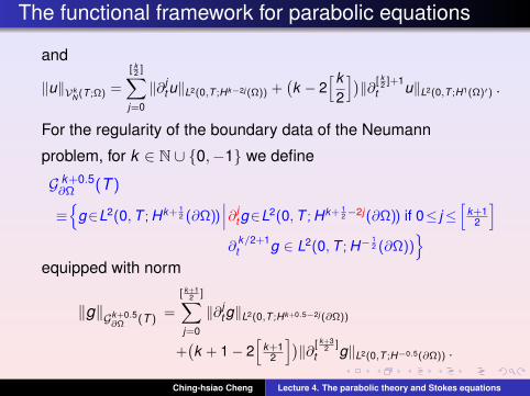
‖u‖VkN (T ;Ω) =
[ k2 ]∑
j=0
‖∂ jt u‖L2(0,T ;Hk−2j (Ω)) +
(k − 2
[k2
])‖∂[ k
2 ]+1t u‖L2(0,T ;H1(Ω)′) .
For the regularity of the boundary data of the Neumann
problem, for k ∈ N ∪ 0,−1 we define
G k+0.5∂Ω (T )
≡
g∈L2(0,T ; Hk+ 12 (∂Ω))
∣∣∣∂ jt g∈L2(0,T ; Hk+ 1
2−2j (∂Ω)) if 0≤ j≤[
k+12
]∂
k/2+1t g ∈ L2(0,T ; H−
12 (∂Ω))
equipped with norm
‖g‖Gk+0.5∂Ω (T ) =
[ k+12 ]∑
j=0
‖∂ jt g‖L2(0,T ;Hk+0.5−2j (∂Ω))
+(k + 1− 2
[k+1
2
])‖∂[ k+3
2 ]t g‖L2(0,T ;H−0.5(∂Ω)) .
Ching-hsiao Cheng Lecture 4. The parabolic theory and Stokes equations

The regularity theory for parabolic equations
Theorem
Assume that ∂Ω is of class Cm+2, ∂t + L is uniformly parabolic,
aij ,bi , c ∈ Cm+1(Ω× [0,T ]), and[aij] is symmetric. Then for
any u0 ∈ Hm+1(Ω) ∩ H10 (Ω), f ∈ Vm
D (T ; Ω), the unique weak
solution u to the parabolic initial-boundary value problem (D) in
fact belongs to Vm+2D (T ; Ω) and satisfies
‖u‖Vm+2D (T ;Ω) ≤ C
[‖u0‖Hm+1(Ω) + ‖f‖Vm
D (T ;Ω)
],
provided that the compatibility conditions are valid up to([m2
]+ 1)-th order.
Ching-hsiao Cheng Lecture 4. The parabolic theory and Stokes equations

The regularity theory for parabolic equations
Theorem
Assume that ∂Ω is of class Cm+2, ∂t + L is uniformly parabolic,
aij ,bi , c ∈ Cm+1(Ω× [0,T ]), and[aij] is symmetric. Then for
any u0 ∈ Hm+1(Ω), f ∈ VmN (T ; Ω), g ∈ G m+0.5
∂Ω (T ), the unique
weak solution u to the parabolic initial-boundary value problem
(N) in fact belongs to Vm+2N (T ; Ω) and satisfies
‖u‖Vm+2N (T ;Ω) ≤ C
[‖u0‖Hm+1(Ω) + ‖f‖Vm
N (T ;Ω) + ‖g‖Gm+0.5∂Ω (T )
],
provided that the compatibility conditions are valid up to[m + 12
]-th order.
Ching-hsiao Cheng Lecture 4. The parabolic theory and Stokes equations

The regularity theory for parabolic equations
Let Ω = S1 × (0,1) so that ∂Ω = x2 = 0 ∪ x2 = 1, and we
consider
ut −∆u = f in Ω× (0,T ),
u = u0 on Ω× t = 0, (U)
u = 0 on ∂Ω× (0,T ).
Suppose that f ∈ L2(0,T ; H2(Ω)) with ft ∈ L2(0,T ; L2(Ω)), and
u0 ∈ H3(Ω) satisfies the first and the second order compatibility
conditions; that is,
u0 ∈ H10 (Ω) and u1 ≡ f (0) + ∆u0 ∈ H1
0 (Ω).
We show that u ∈ L2(0,T ; H4(Ω)) with ut ∈ L2(0,T ; H2(Ω)) and
utt ∈ L2(0,T ; L2(Ω)).
Ching-hsiao Cheng Lecture 4. The parabolic theory and Stokes equations

The regularity theory for parabolic equations
Let w be the weak solution towt −∆w = ft in Ω× (0,T ),
w = u1 on Ω× t = 0, (W)
w = 0 on ∂Ω× (0,T ).
We note that since u1 ∈ H10 (Ω) and ft ∈ L2(0,T ; L2(Ω)), the
existence of the weak solution is guaranteed by the former
result.
Testing the equation against wt , we find that
‖wt‖2L2(Ω) +
12
ddt‖∇w‖2
L2(Ω) ≤ ‖ft‖L2(Ω)‖wt‖L2(Ω)
thus Young’s inequality implies that
‖wt‖2L2(Ω) +
ddt‖∇w‖2
L2(Ω) ≤ ‖ft‖2L2(Ω)
Ching-hsiao Cheng Lecture 4. The parabolic theory and Stokes equations

The regularity theory for parabolic equations
Therefore, w ∈ L∞(0,T ; H1(Ω)) and wt ∈ L2(0,T ; L2(Ω))
satisfying that
maxt∈[0,T ]
‖w(t)‖2H1(Ω) +
∫ T
0‖wt (t)‖2
L2(Ω)dt ≤ ‖u1‖2H1(Ω) + ‖ft‖2
L2(0,T ;L2(Ω)).
The elliptic estimates further suggest that ‖w(t)‖2L2(0,T ;H2(Ω))
shares the same upper bound.
In order to show that u ∈ L2(0,T ; H4(Ω)), we need to show that
ut ∈ L2(0,T ; H2(Ω)). To see this, we only need to show that
w = ut ; nevertheless, integrating the weak formulation of (W) in
time over the time interval (0, t),
Ching-hsiao Cheng Lecture 4. The parabolic theory and Stokes equations
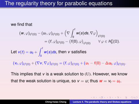
The regularity theory for parabolic equations
we find that
(w , ϕ)L2(Ω) − (u1, ϕ)L2(Ω) +(∇∫ t
0w(s)ds,∇ϕ
)L2(Ω)
= (f , ϕ)L2(Ω) −(f (0), ϕ
)L2(Ω)
∀ ϕ ∈ H10 (Ω).
Let v(t) = u0 +
∫ t
0w(s)ds, then v satisfies
(vt , ϕ)L2(Ω) + (∇v ,∇ϕ)L2(Ω) = (f , ϕ)L2(Ω) + (u1 − f (0)−∆u0, ϕ)L2(Ω).
This implies that v is a weak solution to (U). However, we know
that the weak solution is unique, so v = u; thus w = vt = ut .
Ching-hsiao Cheng Lecture 4. The parabolic theory and Stokes equations

The regularity theory for parabolic equations
Remark: If Ω = Tn, then in principle one can test the equation
against ∆3u to obtain that
12
ddt‖∇∆u‖2
L2(Tn) + ‖∆2u‖2L2(Tn) ≤ ‖∆f‖L2(Tn)‖∆2u‖L2(Tn)
which, together with Young’s inequality, further implies that
ddt‖∇∆u‖2
L2(Tn) + ‖∆2u‖2L2(Tn) ≤ ‖f‖
2H2(Tn)
Therefore, if f ∈ L2(0,T ; H2(Tn)) (but without assuming that
ft ∈ L2(0,T ; L2(Tn))), one conclude that u ∈ L∞(0,T ; H3(Tn))
and u ∈ L2(0,T ; H4(Tn)).
Ching-hsiao Cheng Lecture 4. The parabolic theory and Stokes equations

The time dependent Stokes problem
Let u : Ω→ Rn and p : Ω→ R denote the fluid velocity and
pressure, respectively. We consider
ut −∆u +∇p = f in Ω× (0,T ),
divu = 0 in Ω× (0,T ),
u = u0 on Ω× t = 0,u = 0 on ∂Ω× (0,T ).
(S)
Recall that
H10,div(Ω) =
u ∈ H1
0 (Ω;Rn)∣∣∣ divu = 0
.
Similar to the weak formulation to the parabolic equations and
the steady Stokes equations, we have the following
Ching-hsiao Cheng Lecture 4. The parabolic theory and Stokes equations

The time dependent Stokes problem
Definition
A vector-valued function u ∈ L2(0,T ; H10,div(Ω)) with time
derivative ut ∈ L2(0,T ; H10,div(Ω)′) is said to be a weak solution
to the Stokes equations (S) if
〈ut , ϕ〉+ (∇u,∇ϕ)L2(Ω;Rn2 )= (f , ϕ)L2(Ω;Rn) ∀ ϕ∈H1
0,div(Ω), a.e. t ∈ (0,T )
andu = u0 on Ω× t = 0.
The integral equality is called the variational formulation of the
Stokes equations (S).
Ching-hsiao Cheng Lecture 4. The parabolic theory and Stokes equations

The time dependent Stokes problem
Let L2div(Ω) denote the collection of functions u in L2(Ω;Rn)
such that divu = 0.
Theorem
For any u0 ∈ L2div(Ω) and f ∈ L2(0,T ; L2(Ω;Rn)), there exists a
unique weak solution u to the Stokes equations (S).
The proof of this theorem is almost identical to the existence
and uniqueness of the weak solution to the parabolic equations,
except that the Stokes problem is vector-valued, and we need
to use H10,div(Ω) basis in the Galerkin method.
The existence of p is guaranteed by the Lagrange multiplier
lemma.
Ching-hsiao Cheng Lecture 4. The parabolic theory and Stokes equations

The regularity theory of the Stokes equations
Since the time dependent Stokes equations looks very similar
to the parabolic equation, we would expect similar regularity
theory for the time dependent Stokes equations, as well as the
need of the compatibility conditions. To fully describe the
compatibility conditions, the initial state of the time derivatives
of u have to be computed, while this involves the computation
of the initial state of the time derivatives of p. For example,
ut (0) must satisfy
u1 ≡ ut (0) = ∆u0 −∇p(0) + f (0) in Ω;
thus we need to know how p(0) is obtained in order to proceed.
Ching-hsiao Cheng Lecture 4. The parabolic theory and Stokes equations

The regularity theory of the Stokes equations
Nevertheless, taking the divergence and the normal trace of the
Stokes equations, we find that p(0) solves the elliptic equation
−∆p(0) = divf (0) in Ω,
∂p(0)
∂N= f (0) · N + ∆u0 · N on ∂Ω.
When u0 ∈ Hm(Ω;Rn) ∩ H10,div(Ω) for some m ≥ 2, the solution
p0 ∈ L2(Ω)/R is uniquely determined by the equation.
In general, we have the following
Ching-hsiao Cheng Lecture 4. The parabolic theory and Stokes equations

The regularity theory of the Stokes equations
Definition
For k ∈ N, with pk−1 defined by
−∆pk−1 = div(∂k−1t f )(0) in Ω,
∂pk−1
∂N=[(∂k−1
t f )(0) + ∆uk−1]· N on ∂Ω,
the initial state of the k -th time derivative of u is given by
uk ≡ ∂kt |t=0u = ∆uk−1 −∇pk−1 + (∂k
t f )(0).
By elliptic regularity, for 1 ≤ k ≤[m+1
2
],
[ m+12 ]∑
k=1
[‖uk‖Hm+1−2k (Ω) + ‖pk−1‖Hm+2−2k (Ω)
]≤ C
[‖u0‖Hm+1(Ω) +
[ m+12 ]∑
k=0
‖∂kt f‖L2(0,T ;Hm−2k (Ω))
].
Ching-hsiao Cheng Lecture 4. The parabolic theory and Stokes equations

The regularity theory of the Stokes equations
Definition
For k ∈ N ∪ 0, the (k + 1)-th order compatibility condition forthe time dependent Stokes equations (S) is uk = 0 on ∂Ω.
Theorem
Assume that ∂Ω is of class Cm+2 for some m ∈ N ∪ 0. Thenfor any u0 ∈ Hm+1(Ω;Rn) ∩ H1
0,div(Ω) and f ∈ VmD (T ; Ω), the
unique weak solution u to the Stokes equations (S) in factbelongs to Vm+2
D (T ; Ω) and satisfies
‖u‖Vm+2D (T ;Ω) ≤ C
[‖u0‖Hm+1(Ω) + ‖f‖Vm
D (T ;Ω)
],
provided that the compatibility conditions are valid up to([m2
]+ 1)-th order.
Ching-hsiao Cheng Lecture 4. The parabolic theory and Stokes equations

The decay of the solution to the Stokes equations
Before proceeding, we introduce the space Vs defined by
Vs =
u ∈ Hs(Tn;Rn)∣∣∣ ∫
Tnu(x) dx = 0
.
For any u0 ∈ Vs, we denote etAu0 as the solution u to
ut −∆u +∇p = 0 in Tn × (0,T ),
divu = 0 in Tn × (0,T ),
u = u0 on Tn × t = 0.
Lemma
‖etA‖B(Vs,Vs+1) ≤ Ct−12 for t ∈ (0,1]; that is,
‖etAu0‖Vs+1 ≤ Ct−12 ‖u0‖Vs ∀ u0 ∈ Vs.
Ching-hsiao Cheng Lecture 4. The parabolic theory and Stokes equations

The decay of the solution to the Stokes equations
Proof: Since Tn is a domain without boundary, the regularity
theory of the Stokes equation suggests that u = etAu0 ∈ Vs+1.
Moreover,12
ddt‖Dk u‖2
L2(Tn) + ‖∇Dk u‖2L2(Tn) = 0;
thus12
ddt‖u‖2
Hs(Tn) + ‖u‖2Hs+1(Tn) = 0.
Therefore,
2∫ t
0‖u(t)‖2
Hs+1(Tn)dt = ‖u0‖2Hs(Tn) − ‖u(t)‖2
Hs(Tn) ≤ ‖u0‖2Hs(Tn).
Ching-hsiao Cheng Lecture 4. The parabolic theory and Stokes equations

The decay of the solution to the Stokes equations
On the other hand, the Poincare inequality further implies that
ddt‖u‖2
Hs(Tn) ≤ −C‖u‖2Hs(Tn)
for some constant C > 0. As a consequence,
‖u(t)‖2Hs+1(Tn) ≤ e−C(t−r)‖u(r)‖2
Hs+1(Tn).
Integrating the inequality above in r over the time interval (0, t),
we conclude that
t‖u(t)‖2Hs+1(Tn) ≤
∫ t
0‖u(r)‖2
Hs+1(Tn) ≤12‖u0‖2
Hs(Tn).
Ching-hsiao Cheng Lecture 4. The parabolic theory and Stokes equations
Related Documents


