Lecture 3: Confidence intervalskeshet/MCB2012/SlidesDodo/DataFitLect3.pdf · Bootstrap confidence intervals: Computational technique based on resampling the errors. Asymptotic confidence

Experimental data analysisLecture 3: Confidence intervals

Dodo Das

Review of lecture 2

Nonlinear regression - Iterative likelihood maximization

Levenberg-Marquardt algorithm (Hybrid of steepest descent and Gauss-Newton)

Stochastic optimization - MCMC, Simulated annealing.

Figure 3: Overview of fitting data to a model. A) Simulated dose-response data (solid circles) generated from aHill function (equation 1) using parameter values Emax = 0.8, LEC50 = !1.0, and n = 2, and with normallydistributed noise (with a standard deviation of 0.15) added to mimic experimental error. The best-fit curve (solidline) is obtained from nonlinear least squares regression between the data and a Hill function (equation 1). SeeTable 1 for the best-fit parameter estimates. Nonlinear data fitting algorithms work by finding the model parametersthat minimize the distance between the data and the curve. The distance is measured as the sum of squared residuals(SSR), where the residuals are the distance between the data and the curve. B) Residuals between the best fit curveand the data shown in panel A. C) Heat map of the SSR as a function of EC50 and Emax along with the path takenby the SSR minimization algorithm terminating at the best-fit estimate (red line) which lies near the minimum of theSSR landscape.

Figure 4: Bootstrap distribution and confidence intervals for the parameter estimates shown in Table 1 Missingy-axix, add panel labels, add panel captions.

A B C D

0.8

0.85

0.9

0.95

1

Emax

0

1

2

3

4

5

6

n

!2

!1.5

!1

!0.5

LEC

50

Figure 5: Determining statistical differences between two curves using a Bonferroni corrected t-test. A) Two sim-ulated dose-response curves (colored circles) are shown. We wish to determine if these two curves are statisticallydifferent. To do this, we fit the standard three parameter Hill function to the curve (solid lines). We find excellentfits with R2 = 0.89 (blue) and R2 = 0.95 (red). B-D) Estimates of Emax, EC50 and n are shown along with theirstandard errors for the two curves. Based on the values and the standard error, we expect statistical differences inEC50 but not in n and Emax. This is indeed reflected in the Bonferroni corrected t-test, see Table 3. Simulated dose-response curves are generated by adding normally distributed noise (with ! = 0.15) to the standard three parameterHill function with Emax = 0.9, EC50 = 10!1.5, n = 1.0 (blue curve) and Emax = 1.0, EC50 = 10!0.5, n = 2.0 (redcurve).

20

Demo 3: Nonlinear regression in MATLAB

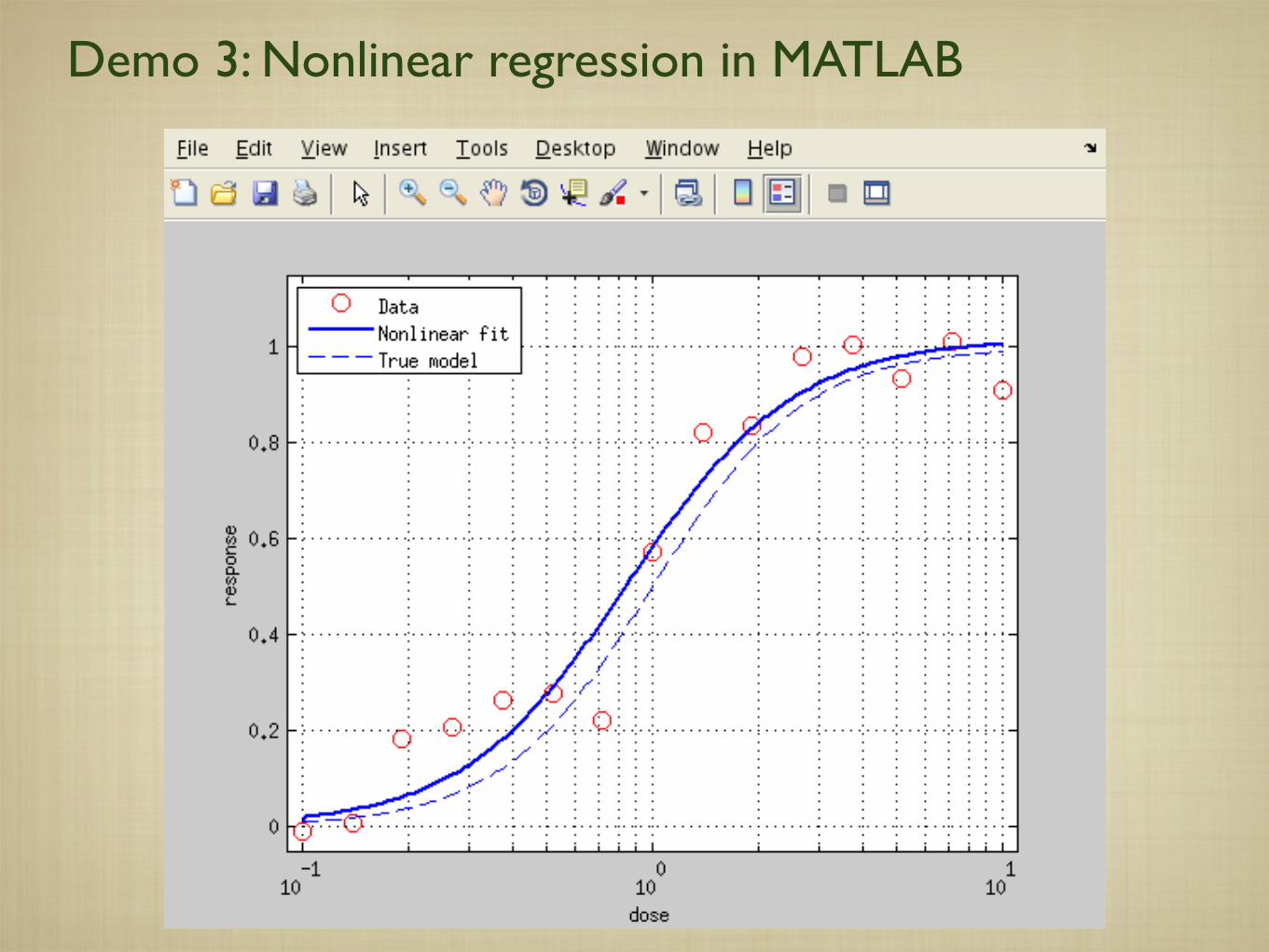
Objective: Using a Hill function to model dose-response data.

Figures

A B C

Figure 1: Examples of dose-dependent or time-dependent data to be compared. A) Dose-response data for T cellactivation. T cells were incubated with two different ligands at indicated doses for 4 hours, and the concentration ofIFN-! (a secreted cytokine) in the supernatant was measured. Data adapted from Dushek et al [1]. B) Fluorescencerecovery after photobleaching (FRAP) data for Grip-75, a component of the pericentriolar material (PCM). Thenormalized fluorescence intensity is measured as a function of time at the centre and at the periphery of the PCM.Data adapted from Conduit et al [7]. C) Binding titration of two PEGylated ligands for IgE, showing fraction of IgEbinding sites that are occupied as a function of the ligand concentration. Data adapted from Das et al [2].

Figure 2: The effect of independently varying each of the three parameters of a Hill function. Many dose-responseexperiments are well fitted by a Hill function with three parameters: the maximal response (Emax), the dose (EC50)for half-maximal response, and the Hill number (n) that measures the steepness (sensitivity) of the response. Thethree panels show how the dose-response changes when each of the parameters is independently varied: A) EC50from 0.1 to 10, B) Emax from 0.1 to 1, and C) n from 0.5 to 4. In each case, the parameter values, Emax = 1,EC50 = 1, and n = 2 give rise to the default dose response curve (bold black line). Note that the parameters areindependent so that, for example, a change in n does not alter EC50 or Emax (panel c).

19


Need the statistics toolbox which contains the function nlinfit

i) Write a MATLAB function to compute the Hill function for a given set of parameter values.


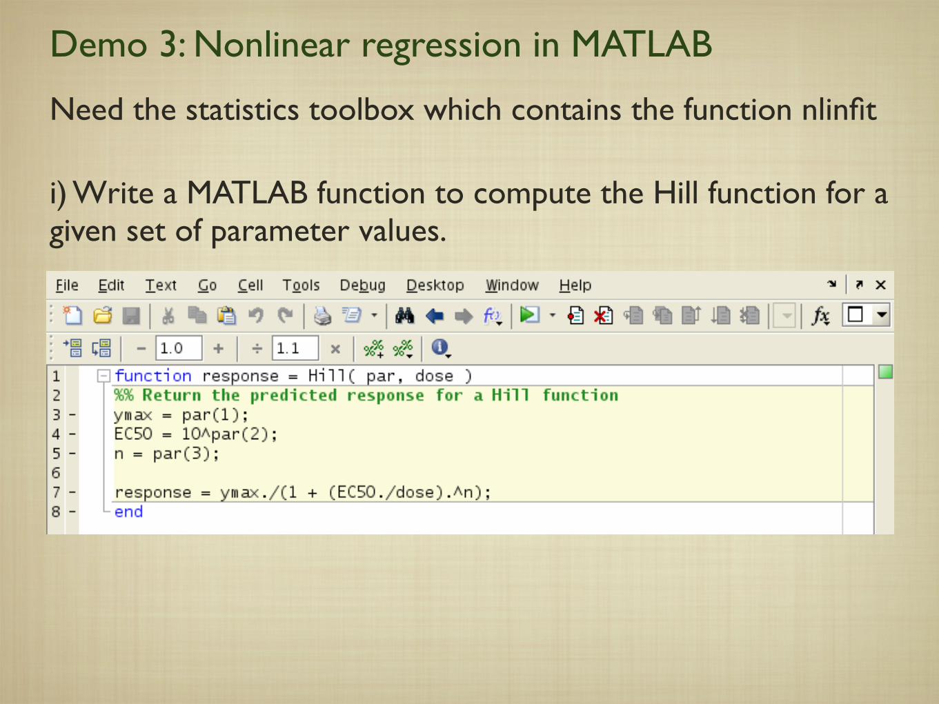
ii) Choose some model parameters to simulate data [or collect data from experiments]


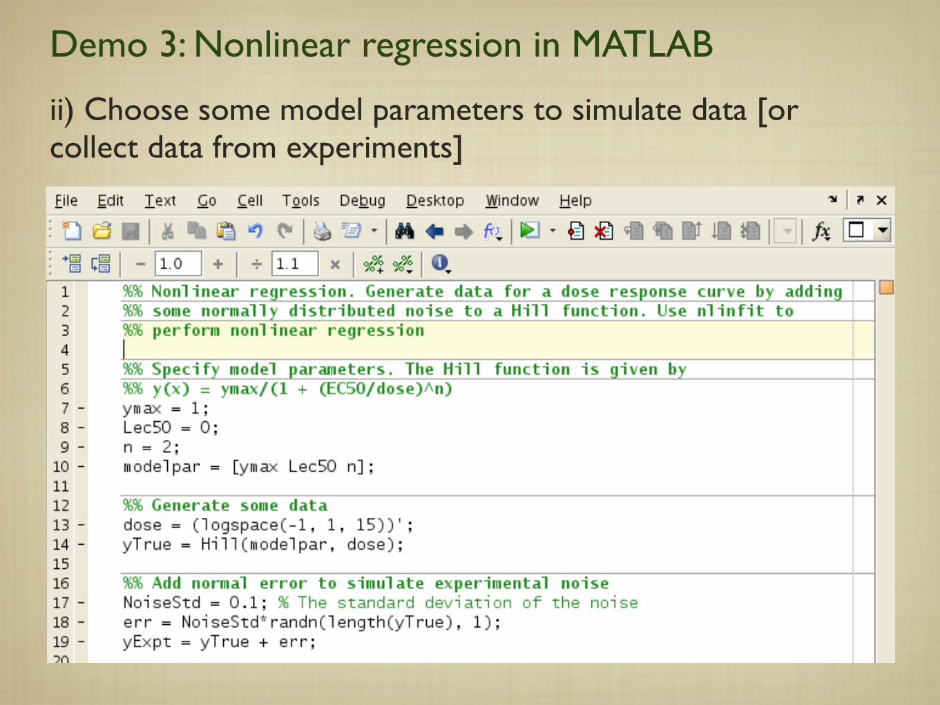
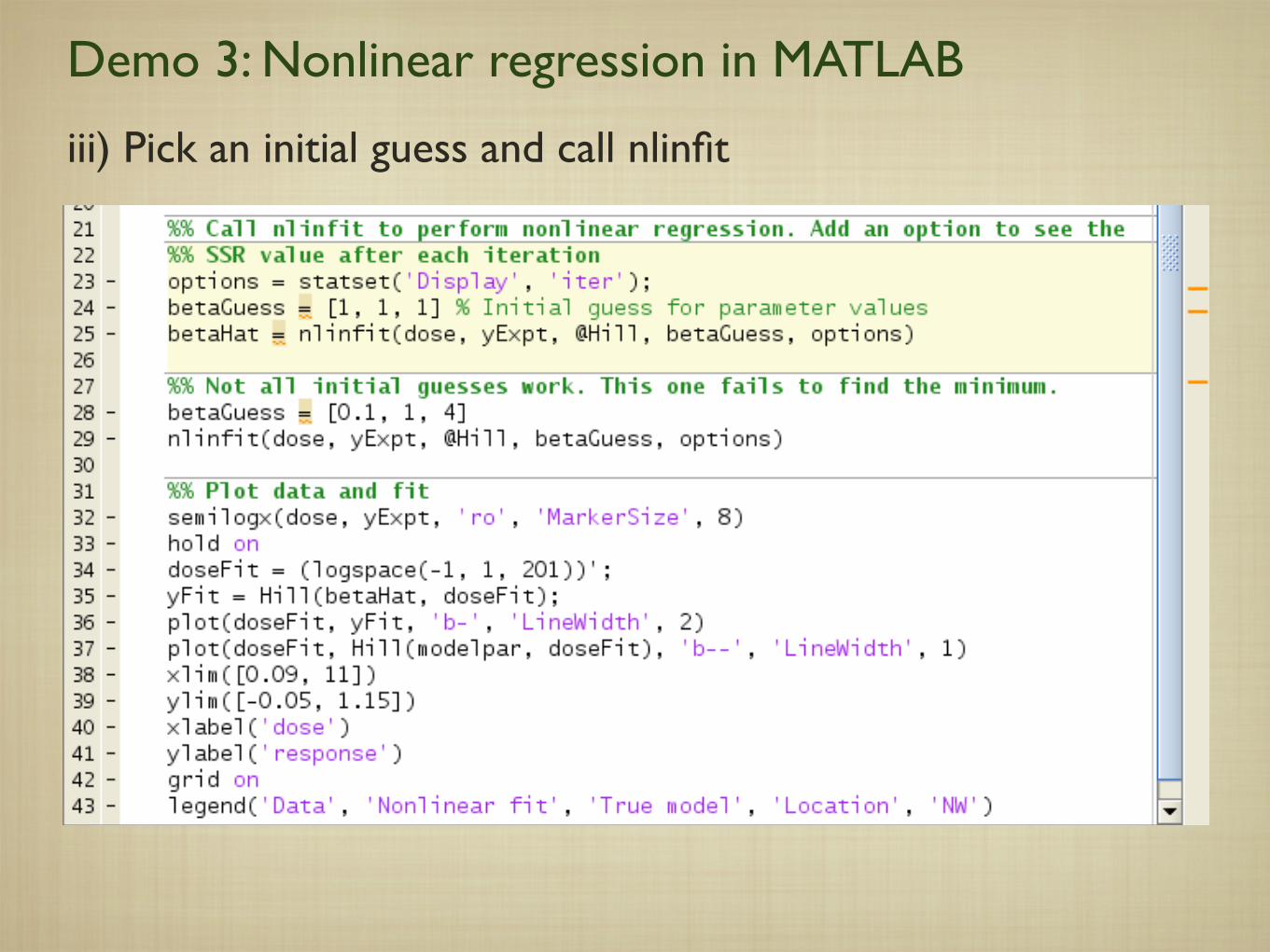
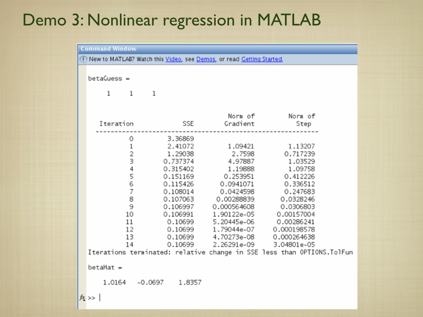
iii) Pick an initial guess and call nlinfit




Convergence can be sensitive to the initial guess.


Convergence can be sensitive to the initial guess.


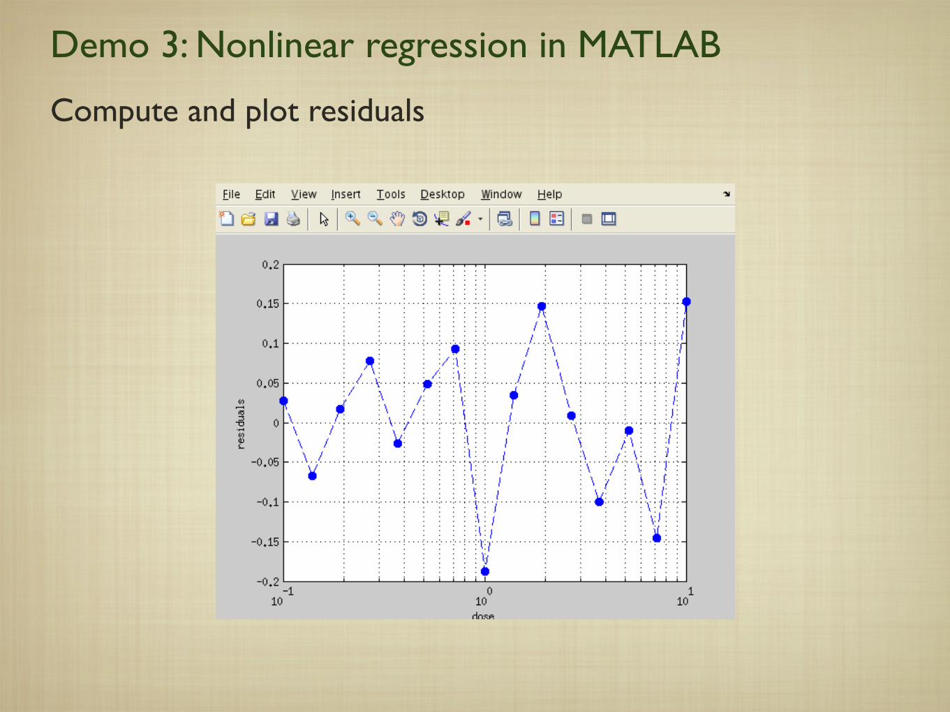
Compute and plot residuals

Parameter confidence intervals

Question: What does a 95% confidence interval mean?

eg: Say, a best fit parameter estimate is â = 1, and we have estimated the 95% CI to be [0.5, 1.5]. How can we interpret this result?

Parameter confidence intervals

Question: What does a 95% confidence interval mean?

eg: Say, a best fit parameter estimate is â = 1, and we have estimated the 95% CI to be [0.5, 1.5]. How can we interpret this result?

If we repeat our experiment and the fitting procedure many times, 95% of the times the true (but unknown) parameter value will lie within this CI.

Computing parameter confidence intervals

Two approaches:

1. Asymptotic confidence intervals: Based on an analytical approximation.

2. Bootstrap confidence intervals: Computational technique based on resampling the errors.

Asymptotic confidence intervals

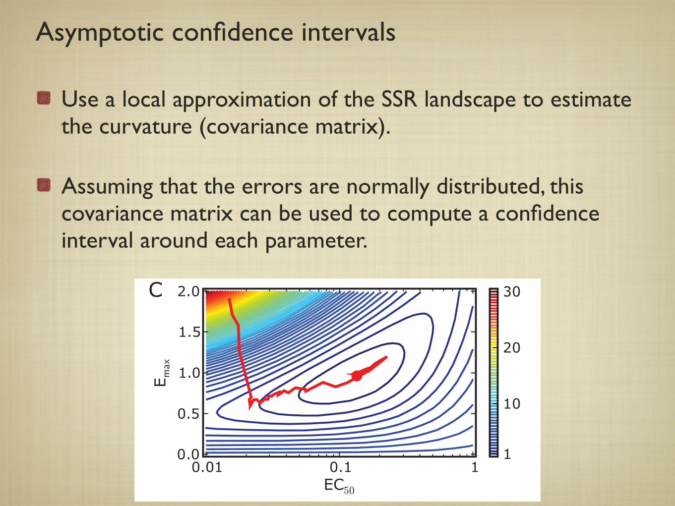
Use a local approximation of the SSR landscape to estimate the curvature (covariance matrix).

Assuming that the errors are normally distributed, this covariance matrix can be used to compute a confidence interval around each parameter.



A B C D

0.8

0.85

0.9

0.95

1

Emax

0

1

2

3

4

5

6

n

!2

!1.5

!1

!0.5

LEC

50


20

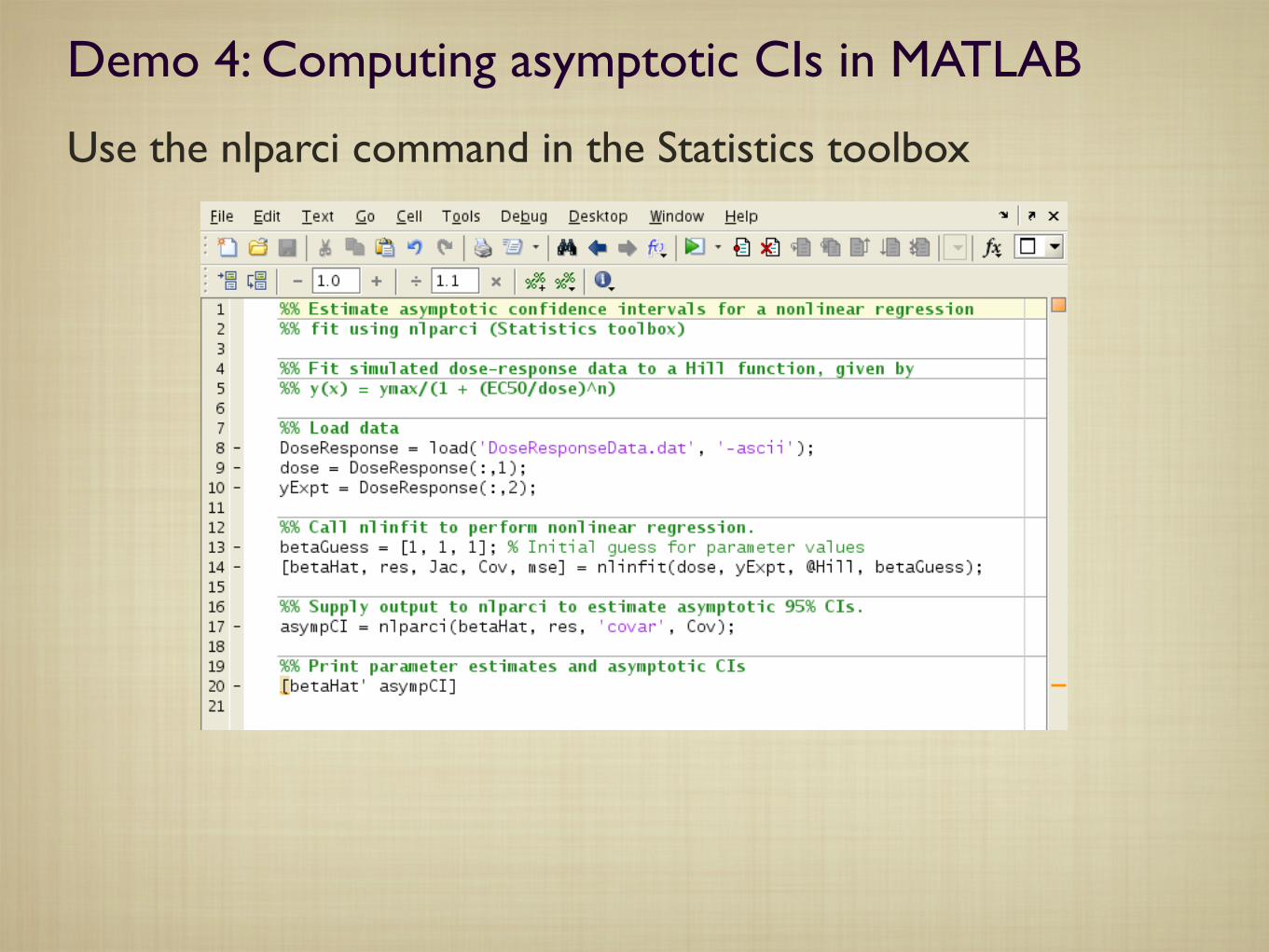
Demo 4: Computing asymptotic CIs in MATLAB

Use the nlparci command in the Statistics toolbox

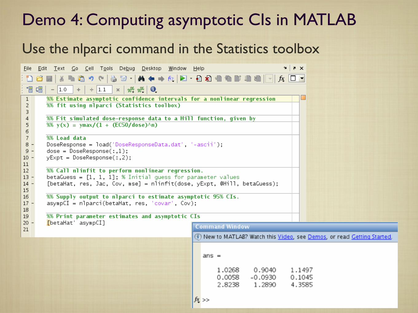
Demo 4: Computing asymptotic CIs in MATLAB

Use the nlparci command in the Statistics toolbox

Bootstrapping: The principle

A computational approach that addresses the following question:

Given a limited number of observations, how can we estimate some quantity, eg: mean, median etc. for the population from which the observations are drawn?

If we ‘resample’ from the observations, we can, in some sense, simulate the population distribution.

Bootstrapping in practice for nonlinear regression.

is related to the distribution of experimental noise. In fact, it can be shown that if the errors are normally distributed,then the parameter estimates are also approximately normally distributed. And the standard deviations of thesedistributions are usually reported as the standard error of the parameter estimates.

Is it really true that the standard deviations are reported as the standard error? (Last line inabove paragraph). Dodo: I am pretty sure that this is the case. I can verify this after I get backfrom India.

Another commonly used measure of the uncertainty in parameter estimates is a 95% confidence interval (CI). Givena 95% CI for a parameter, the interpretation is that 95% of the times this CI will enclose the true parameter value.Therefore, a narrow confidence interval means that we can be fairly confident that the true parameter value is closeto its best fit estimate, while a wide confidence interval means that there could be a large discrepancy between thetrue value of the parameter and its best fit estimate.

2.5.1 Bootstrap CI

There are two commonly used estimates of parameter CIs: an asymptotic CI, and a bootstrap CI. Asymptotic CIsare based on the standard deviations of the parameter estimates, and as such, assume that the experimental erroris normally distributed. Bootstrap CIs do not make this assumption, and are therefore more general. In particular,bootstrap estimates are more reliable for small data sets. Asymptotic CIs are usually included in the output of mostdata fitting routines whereas bootstrap CIs are not. Below, we describe the procedure for generating bootstrap CIs.

Bootstrapping is a statistical technique for computing standard errors and confidence intervals of estimated param-eters. The major advantages of bootstrapping are its conceptual simplicity and its applicability to small data sets.However, bootstrapping is not commonly implemented as a standard tool in data analysis packages. Therefore,generating bootstrap estimates requires some additional work on part of the user. It is also more computationally ex-pensive compared to the asymptotic methods, but this is rarely a limitation with the availability of modern computingpower.

To understand bootstrapping, it is helpful to view the data fitting procedure in a somewhat abstract manner. Weassume that observed data arise from an ‘ideal’ response plus some noise or experimental error that obeys somestatistical distribution. Our goal is to estimate the parameters that define the ideal response. Typically, we knownothing about the error distribution. In an ideal world, we would have the luxury of repeating an experiment many,many times over, each time obtaining an independent replicate of the data. These independent replicates would, ina sense, allow us to reconstruct the unknown error distribution, and therefore precisely quantify the uncertainty inour estimates of model parameters. In the real world, of course, experiments are expensive and data is precious. So,we resort to a computational procedure that approximates the strategy of repeating experiments: we resample theobserved errors to simulate replicate data sets.

Here is how the bootstrapping procedure works in practise for a nonlinear regression problem:

1. Use the nonlinear least squares regression to determine the best-fit estimates of the model parameters, and thepredicted model response (yi)predicted at each value of the independent variable xi.

2. Calculate the residuals !i = (yi)observed ! (yi)predicted at each of the N data points.

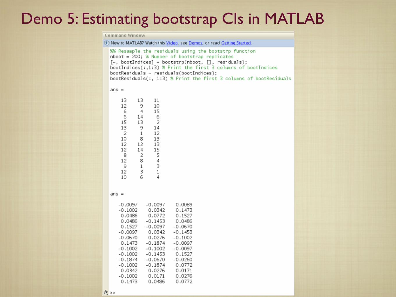
63. Resample the residuals with replacement to generate a new set of residuals {!!i }. What this means is that wegenerate a new set of N residuals where each of N values is one of the original residuals chosen with equalprobability. Typically, some of the original residuals will be chosen more than once, while some will not bechosen at all. For example, say we have three data points and we calculate the residuals to be 0.1, -0.2 and0.3. Then some possible sets of resampled residuals are: {-0.2, 0.1, -0.2}, {0.1, 0.3, -0.2}, {0.3, -0.2, -0.2},and so on.

4. Add the resampled residuals to the predicted response to generate a bootstrap data set, {xi, y!i } = {xi, (yi)predicted+!!i }

5. Treat the bootstrap dataset as an independent replicate experiment, and fit it to the model to calculate newestimates of model parameters.

6. Repeat steps 3-5 many times - typically 500 to 1000 times - each time generating a new bootstrap data set, andfitting it to the model. Store the resulting best-fit parameter estimates. These independent estimates constitutea sample from the bootstrap distribution of the model parameters.

7. For each parameter, calculate the standard deviation of the bootstrap sample. This standard deviation is theestimated bootstrap standard error for that parameter.

8. To calculate the 95% bootstrap CIs, compute the 97.5th and the 2.5th percentile values of each parameter fromthe bootstrap distributions. (There are other prescriptions for calculating bootstrap CIs, but this one is thesimplest.)

The origin of the name ‘bootstrapping’ should now make sense. We are generating the independent replicates byintelligently using our original data - reminiscent of a person pulling themselves up by their bootstrap. In Fig. 4,we plot histograms of the bootstrap parameter distribution from fitting bootstrap replicates of the dose response datain Fig. 3, overlaid with the 95% bootstrap CIs. Note that the bootstrap distributions and CIs are not necessarilysymmetric about the best-fit estimates. This is in contrast with the asymptotic CIs which are based on a normaldistribution which is symmetrical about the mean.

Should we explicitly relate the standard deviation to the CI? In other words, the probability thatthe parameters are within 1 standard deviation of their true values is 68.2%.Dodo: I wouldn’t bother. It’s too technical a detail, given the target audience for this tutorial. (Imight change my mind after I read the final draft.)

Table 2: Asymptotic and bootstrap confidence intervals for data in Fig. 3.

Parameter True value Best-fit Standard error 95% CIestimate Asymptotic Bootstrap Asymptotic Bootstrap

Emax 0.8 0.96 0.090 0.090 [0.77, 1.2] [0.79, 1.1]LEC50 -1.0 -0.87 0.082 0.091 [-1.0, -0.69] [-1.0, -0.63]n 2 1.8 0.46 0.502 [0.80, 2.8] [1.1, 3.1]

7

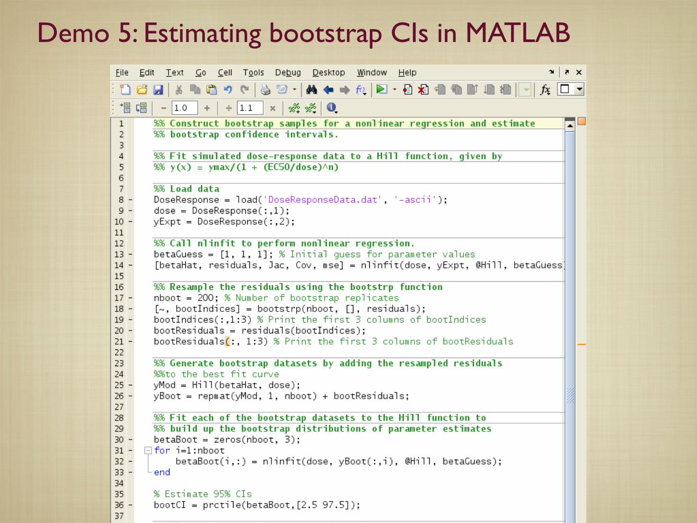
Demo 5: Estimating bootstrap CIs in MATLAB




Comparing fits from two different experiments



A B C D

0.8

0.85

0.9

0.95

1

Emax

0

1

2

3

4

5

6

n

!2

!1.5

!1

!0.5

LEC

50


20

Which paramters are different between the two datasets?

Bootstrap-based hypothesis testing

Figure 6: Bootstrap distibutions for comparing the two datasets shown in Figure 5

0.01 0.1 1

0

0.5

1R2=0.81 m=2

R2=0.93 m=3

x (dose)

y (r

esp

on

se)

Figure 7: Comparing the fit of two models to a single data set. Simulated data (blue circles) is obtained by adding15% normally distributed noise to a dose-response curve with B = 0, Emax = 1, EC50 = 10!1.0, and n = 4. Thetwo proposed models we will consider are the reduced Hill function (equation 2), that contains two fitting parameters(EC50 and Emax) with two fixed parameters (B = 0 and n = 1), and a slightly more complicated model (equation1) that contains three fitting parameters (EC50, Emax, and n) with one fixed parameter (B = 0). Given that the twomodels are nested, we expect that the more complicated model will fit the data at least as good as the simpler model.Data fitting of each model to the simulated data does indeed reveal that the more complicated model (solid red line)exhibits a larger R2 value compared to the simpler model (solid blue line). We perform a statistical test (F-test,see main text) for the null hypothesis that the two models fit the data equally well. This test accounts not only forthe SSR of each model but the number of parameters, and we find p = 7.45 ! 10!6. We therefore reject the nullhypothesis and conclude that the simpler model is insufficient to explain the data.

21

Emax is not (the 95% CI of the difference distribution crosses 0), but EC50 and n are different.

Friday

How to pick the best model from a set of proposed models?

Bias-variance tradeoff

F-test

Akaike’s information criterion (AIC)

Lecture 3: Confidence intervalskeshet/MCB2012/SlidesDodo/DataFitLect3.pdf · Bootstrap confidence intervals: Computational technique based on resampling the errors. Asymptotic confidence

Documents