Lecture 20 - Logistic Regression Statistics 102 Colin Rundel April 15, 2013

Welcome message from author
This document is posted to help you gain knowledge. Please leave a comment to let me know what you think about it! Share it to your friends and learn new things together.
Transcript
Lecture 20 - Logistic Regression
Statistics 102
Colin Rundel
April 15, 2013

Background
1 Background
2 GLMs
3 Logistic Regression
4 Additional Example
Statistics 102
Lec 20 Colin Rundel
Background
Regression so far ...
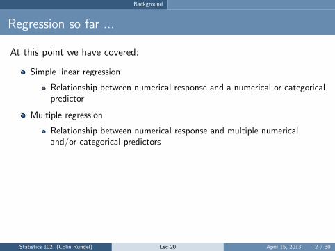
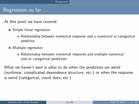
At this point we have covered:
Simple linear regression
Relationship between numerical response and a numerical or categoricalpredictor
Multiple regression
Relationship between numerical response and multiple numericaland/or categorical predictors
What we haven’t seen is what to do when the predictors are weird(nonlinear, complicated dependence structure, etc.) or when the responseis weird (categorical, count data, etc.)
Statistics 102 (Colin Rundel) Lec 20 April 15, 2013 2 / 30
Background
Regression so far ...
At this point we have covered:
Simple linear regression
Relationship between numerical response and a numerical or categoricalpredictor
Multiple regression
Relationship between numerical response and multiple numericaland/or categorical predictors
What we haven’t seen is what to do when the predictors are weird(nonlinear, complicated dependence structure, etc.) or when the responseis weird (categorical, count data, etc.)
Statistics 102 (Colin Rundel) Lec 20 April 15, 2013 2 / 30
Background
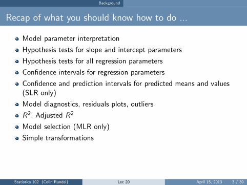
Recap of what you should know how to do ...
Model parameter interpretation
Hypothesis tests for slope and intercept parameters
Hypothesis tests for all regression parameters
Confidence intervals for regression parameters
Confidence and prediction intervals for predicted means and values(SLR only)
Model diagnostics, residuals plots, outliers
R2, Adjusted R2
Model selection (MLR only)
Simple transformations
Statistics 102 (Colin Rundel) Lec 20 April 15, 2013 3 / 30
Background
Odds
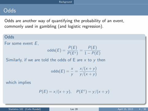
Odds are another way of quantifying the probability of an event,commonly used in gambling (and logistic regression).
Odds
For some event E ,
odds(E ) =P(E )
P(E c)=
P(E )
1− P(E )
Similarly, if we are told the odds of E are x to y then
odds(E ) =x
y=
x/(x + y)
y/(x + y)
which implies
P(E ) = x/(x + y), P(E c) = y/(x + y)
Statistics 102 (Colin Rundel) Lec 20 April 15, 2013 4 / 30

GLMs
1 Background
2 GLMs
3 Logistic Regression
4 Additional Example
Statistics 102
Lec 20 Colin Rundel
GLMs
Example - Donner Party
In 1846 the Donner and Reed families left Springfield, Illinois, for Californiaby covered wagon. In July, the Donner Party, as it became known, reachedFort Bridger, Wyoming. There its leaders decided to attempt a new anduntested rote to the Sacramento Valley. Having reached its full size of 87people and 20 wagons, the party was delayed by a difficult crossing of theWasatch Range and again in the crossing of the desert west of the GreatSalt Lake. The group became stranded in the eastern Sierra Nevadamountains when the region was hit by heavy snows in late October. Bythe time the last survivor was rescued on April 21, 1847, 40 of the 87members had died from famine and exposure to extreme cold.
From Ramsey, F.L. and Schafer, D.W. (2002). The Statistical Sleuth: A Course in Methods of Data Analysis (2nd ed)
Statistics 102 (Colin Rundel) Lec 20 April 15, 2013 5 / 30
GLMs
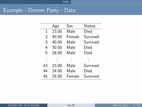
Example - Donner Party - Data
Age Sex Status
1 23.00 Male Died2 40.00 Female Survived3 40.00 Male Survived4 30.00 Male Died5 28.00 Male Died...
......
...43 23.00 Male Survived44 24.00 Male Died45 25.00 Female Survived
Statistics 102 (Colin Rundel) Lec 20 April 15, 2013 6 / 30
GLMs
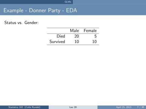
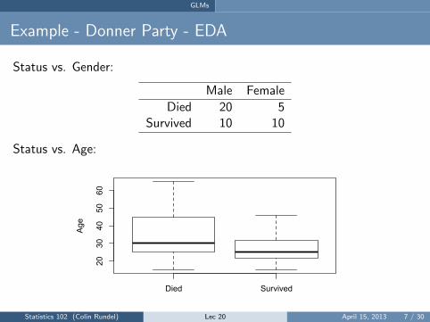
Example - Donner Party - EDA
Status vs. Gender:
Male Female
Died 20 5Survived 10 10
Status vs. Age:
Died Survived
2030
4050
60
Age
Statistics 102 (Colin Rundel) Lec 20 April 15, 2013 7 / 30
GLMs
Example - Donner Party - EDA
Status vs. Gender:
Male Female
Died 20 5Survived 10 10
Status vs. Age:
Died Survived
2030
4050
60
Age
Statistics 102 (Colin Rundel) Lec 20 April 15, 2013 7 / 30

GLMs
Example - Donner Party - ???
It seems clear that both age and gender have an effect on someone’ssurvival, how do we come up with a model that will let us explore thisrelationship?
Even if we set Died to 0 and Survived to 1, this isn’t something we cantransform our way out of - we need something more.
One way to think about the problem - we can treat Survived and Died assuccesses and failures arising from a binomial distribution where theprobability of a success is given by a transformation of a linear model ofthe predictors.
Statistics 102 (Colin Rundel) Lec 20 April 15, 2013 8 / 30
GLMs
Generalized linear models
It turns out that this is a very general way of addressing this type ofproblem in regression, and the resulting models are called generalizedlinear models (GLMs). Logistic regression is just one example of this typeof model.
All generalized linear models have the following three characteristics:
1 A probability distribution describing the outcome variable2 A linear model
η = β0 + β1X1 + · · ·+ βnXn
3 A link function that relates the linear model to the parameter of theoutcome distribution
g(p) = η or p = g−1(η)
Statistics 102 (Colin Rundel) Lec 20 April 15, 2013 9 / 30
Logistic Regression
1 Background
2 GLMs
3 Logistic Regression
4 Additional Example
Statistics 102
Lec 20 Colin Rundel
Logistic Regression
Logistic Regression
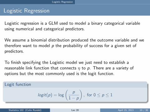
Logistic regression is a GLM used to model a binary categorical variableusing numerical and categorical predictors.
We assume a binomial distribution produced the outcome variable and wetherefore want to model p the probability of success for a given set ofpredictors.
To finish specifying the Logistic model we just need to establish areasonable link function that connects η to p. There are a variety ofoptions but the most commonly used is the logit function.
Logit function
logit(p) = log
(p
1− p
), for 0 ≤ p ≤ 1
Statistics 102 (Colin Rundel) Lec 20 April 15, 2013 10 / 30
Logistic Regression
Logistic Regression
Logistic regression is a GLM used to model a binary categorical variableusing numerical and categorical predictors.
We assume a binomial distribution produced the outcome variable and wetherefore want to model p the probability of success for a given set ofpredictors.
To finish specifying the Logistic model we just need to establish areasonable link function that connects η to p. There are a variety ofoptions but the most commonly used is the logit function.
Logit function
logit(p) = log
(p
1− p
), for 0 ≤ p ≤ 1
Statistics 102 (Colin Rundel) Lec 20 April 15, 2013 10 / 30
Logistic Regression
Properties of the Logit
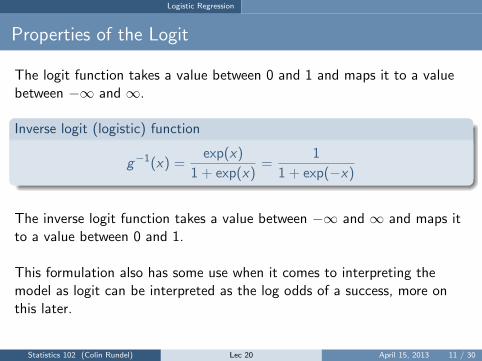
The logit function takes a value between 0 and 1 and maps it to a valuebetween −∞ and ∞.
Inverse logit (logistic) function
g−1(x) =exp(x)
1 + exp(x)=
1
1 + exp(−x)
The inverse logit function takes a value between −∞ and ∞ and maps itto a value between 0 and 1.
This formulation also has some use when it comes to interpreting themodel as logit can be interpreted as the log odds of a success, more onthis later.
Statistics 102 (Colin Rundel) Lec 20 April 15, 2013 11 / 30
Logistic Regression
The logistic regression model
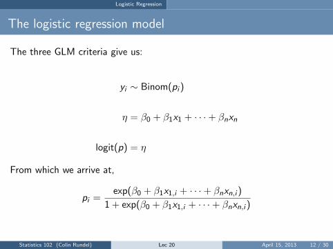
The three GLM criteria give us:
yi ∼ Binom(pi )
η = β0 + β1x1 + · · ·+ βnxn
logit(p) = η
From which we arrive at,
pi =exp(β0 + β1x1,i + · · ·+ βnxn,i )
1 + exp(β0 + β1x1,i + · · ·+ βnxn,i )
Statistics 102 (Colin Rundel) Lec 20 April 15, 2013 12 / 30
Logistic Regression
Example - Donner Party - Model
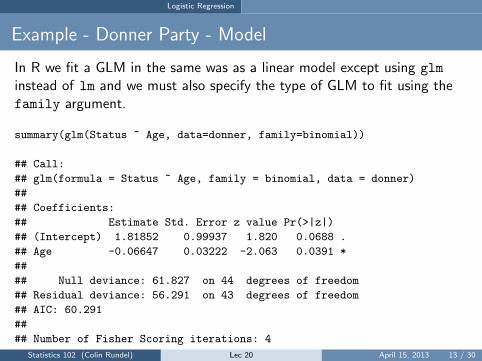
In R we fit a GLM in the same was as a linear model except using glm
instead of lm and we must also specify the type of GLM to fit using thefamily argument.
summary(glm(Status ~ Age, data=donner, family=binomial))
## Call:
## glm(formula = Status ~ Age, family = binomial, data = donner)
##
## Coefficients:
## Estimate Std. Error z value Pr(>|z|)
## (Intercept) 1.81852 0.99937 1.820 0.0688 .
## Age -0.06647 0.03222 -2.063 0.0391 *
##
## Null deviance: 61.827 on 44 degrees of freedom
## Residual deviance: 56.291 on 43 degrees of freedom
## AIC: 60.291
##
## Number of Fisher Scoring iterations: 4
Statistics 102 (Colin Rundel) Lec 20 April 15, 2013 13 / 30
Logistic Regression
Example - Donner Party - Prediction
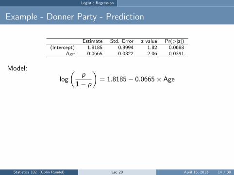
Estimate Std. Error z value Pr(>|z|)(Intercept) 1.8185 0.9994 1.82 0.0688
Age -0.0665 0.0322 -2.06 0.0391
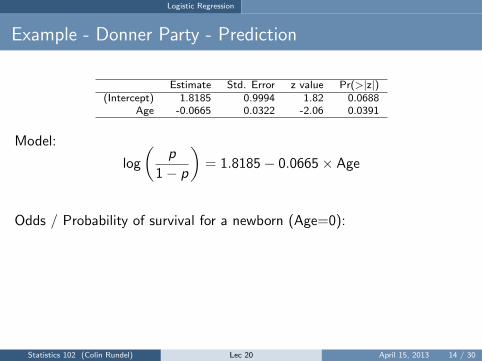
Model:
log
(p
1− p
)= 1.8185− 0.0665× Age
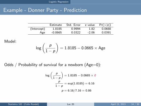
Odds / Probability of survival for a newborn (Age=0):
log
(p
1− p
)= 1.8185− 0.0665× 0
p
1− p= exp(1.8185) = 6.16
p = 6.16/7.16 = 0.86
Statistics 102 (Colin Rundel) Lec 20 April 15, 2013 14 / 30
Logistic Regression
Example - Donner Party - Prediction
Estimate Std. Error z value Pr(>|z|)(Intercept) 1.8185 0.9994 1.82 0.0688
Age -0.0665 0.0322 -2.06 0.0391
Model:
log
(p
1− p
)= 1.8185− 0.0665× Age
Odds / Probability of survival for a newborn (Age=0):
log
(p
1− p
)= 1.8185− 0.0665× 0
p
1− p= exp(1.8185) = 6.16
p = 6.16/7.16 = 0.86
Statistics 102 (Colin Rundel) Lec 20 April 15, 2013 14 / 30
Logistic Regression
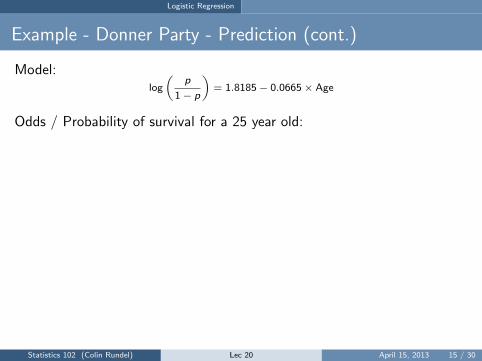
Example - Donner Party - Prediction (cont.)
Model:log
(p
1− p
)= 1.8185− 0.0665× Age
Odds / Probability of survival for a 25 year old:
log
(p
1− p
)= 1.8185− 0.0665× 25
p
1− p= exp(0.156) = 1.17
p = 1.17/2.17 = 0.539
Odds / Probability of survival for a 50 year old:
log
(p
1− p
)= 1.8185− 0.0665× 0
p
1− p= exp(−1.5065) = 0.222
p = 0.222/1.222 = 0.181
Statistics 102 (Colin Rundel) Lec 20 April 15, 2013 15 / 30
Logistic Regression
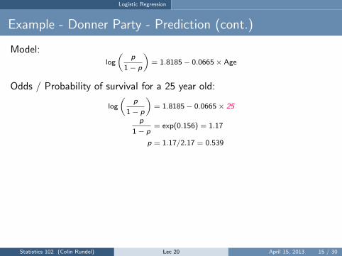
Example - Donner Party - Prediction (cont.)
Model:log
(p
1− p
)= 1.8185− 0.0665× Age
Odds / Probability of survival for a 25 year old:
log
(p
1− p
)= 1.8185− 0.0665× 25
p
1− p= exp(0.156) = 1.17
p = 1.17/2.17 = 0.539
Odds / Probability of survival for a 50 year old:
log
(p
1− p
)= 1.8185− 0.0665× 0
p
1− p= exp(−1.5065) = 0.222
p = 0.222/1.222 = 0.181
Statistics 102 (Colin Rundel) Lec 20 April 15, 2013 15 / 30
Logistic Regression
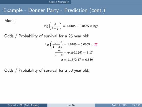
Example - Donner Party - Prediction (cont.)
Model:log
(p
1− p
)= 1.8185− 0.0665× Age
Odds / Probability of survival for a 25 year old:
log
(p
1− p
)= 1.8185− 0.0665× 25
p
1− p= exp(0.156) = 1.17
p = 1.17/2.17 = 0.539
Odds / Probability of survival for a 50 year old:
log
(p
1− p
)= 1.8185− 0.0665× 0
p
1− p= exp(−1.5065) = 0.222
p = 0.222/1.222 = 0.181
Statistics 102 (Colin Rundel) Lec 20 April 15, 2013 15 / 30
Logistic Regression
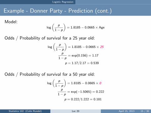
Example - Donner Party - Prediction (cont.)
Model:log
(p
1− p
)= 1.8185− 0.0665× Age
Odds / Probability of survival for a 25 year old:
log
(p
1− p
)= 1.8185− 0.0665× 25
p
1− p= exp(0.156) = 1.17
p = 1.17/2.17 = 0.539
Odds / Probability of survival for a 50 year old:
log
(p
1− p
)= 1.8185− 0.0665× 0
p
1− p= exp(−1.5065) = 0.222
p = 0.222/1.222 = 0.181
Statistics 102 (Colin Rundel) Lec 20 April 15, 2013 15 / 30
Logistic Regression
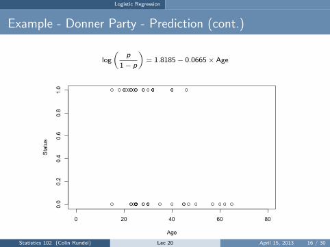
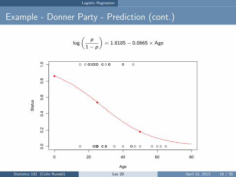
Example - Donner Party - Prediction (cont.)
log
(p
1− p
)= 1.8185− 0.0665× Age
0 20 40 60 80
0.0
0.2
0.4
0.6
0.8
1.0
Age
Status
Statistics 102 (Colin Rundel) Lec 20 April 15, 2013 16 / 30
Logistic Regression
Example - Donner Party - Prediction (cont.)
log
(p
1− p
)= 1.8185− 0.0665× Age
0 20 40 60 80
0.0
0.2
0.4
0.6
0.8
1.0
Age
Status
Statistics 102 (Colin Rundel) Lec 20 April 15, 2013 16 / 30
Logistic Regression
Example - Donner Party - Interpretation
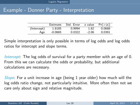
Estimate Std. Error z value Pr(>|z|)(Intercept) 1.8185 0.9994 1.82 0.0688
Age -0.0665 0.0322 -2.06 0.0391
Simple interpretation is only possible in terms of log odds and log oddsratios for intercept and slope terms.
Intercept: The log odds of survival for a party member with an age of 0.From this we can calculate the odds or probability, but additionalcalculations are necessary.
Slope: For a unit increase in age (being 1 year older) how much will thelog odds ratio change, not particularly intuitive. More often then not wecare only about sign and relative magnitude.
Statistics 102 (Colin Rundel) Lec 20 April 15, 2013 17 / 30
Logistic Regression
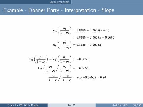
Example - Donner Party - Interpretation - Slope
log
(p1
1− p1
)= 1.8185− 0.0665(x + 1)
= 1.8185− 0.0665x − 0.0665
log
(p2
1− p2
)= 1.8185− 0.0665x
log
(p1
1− p1
)− log
(p2
1− p2
)= −0.0665
log
(p1
1− p1
/p2
1− p2
)= −0.0665
p1
1− p1
/p2
1− p2= exp(−0.0665) = 0.94
Statistics 102 (Colin Rundel) Lec 20 April 15, 2013 18 / 30
Logistic Regression
Example - Donner Party - Age and Gender
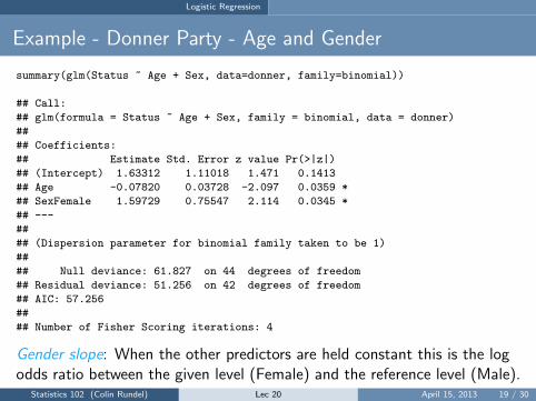
summary(glm(Status ~ Age + Sex, data=donner, family=binomial))
## Call:
## glm(formula = Status ~ Age + Sex, family = binomial, data = donner)
##
## Coefficients:
## Estimate Std. Error z value Pr(>|z|)
## (Intercept) 1.63312 1.11018 1.471 0.1413
## Age -0.07820 0.03728 -2.097 0.0359 *
## SexFemale 1.59729 0.75547 2.114 0.0345 *
## ---
##
## (Dispersion parameter for binomial family taken to be 1)
##
## Null deviance: 61.827 on 44 degrees of freedom
## Residual deviance: 51.256 on 42 degrees of freedom
## AIC: 57.256
##
## Number of Fisher Scoring iterations: 4
Gender slope: When the other predictors are held constant this is the logodds ratio between the given level (Female) and the reference level (Male).
Statistics 102 (Colin Rundel) Lec 20 April 15, 2013 19 / 30
Logistic Regression
Example - Donner Party - Gender Models
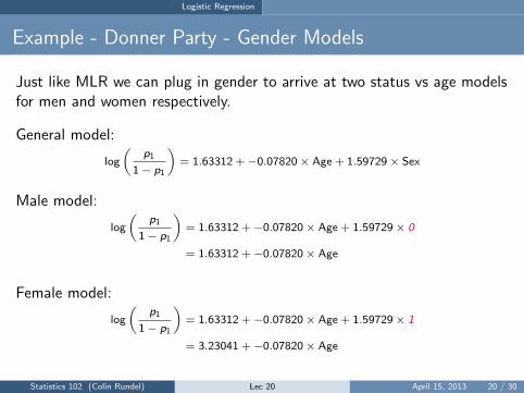
Just like MLR we can plug in gender to arrive at two status vs age modelsfor men and women respectively.
General model:
log
(p1
1− p1
)= 1.63312 +−0.07820× Age + 1.59729× Sex
Male model:
log
(p1
1− p1
)= 1.63312 +−0.07820× Age + 1.59729× 0
= 1.63312 +−0.07820× Age
Female model:
log
(p1
1− p1
)= 1.63312 +−0.07820× Age + 1.59729× 1
= 3.23041 +−0.07820× Age
Statistics 102 (Colin Rundel) Lec 20 April 15, 2013 20 / 30
Logistic Regression
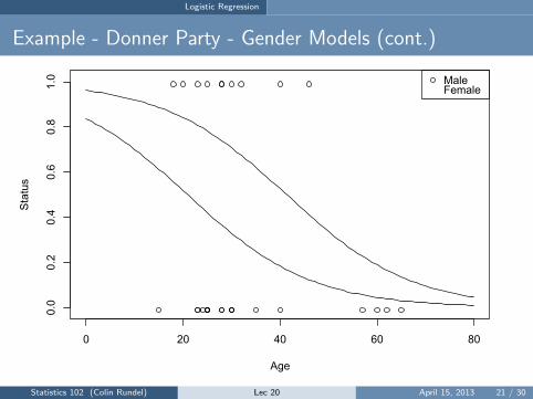
Example - Donner Party - Gender Models (cont.)
0 20 40 60 80
0.0
0.2
0.4
0.6
0.8
1.0
Age
Status
MaleFemale
Statistics 102 (Colin Rundel) Lec 20 April 15, 2013 21 / 30
Logistic Regression
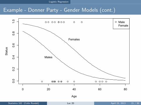
Example - Donner Party - Gender Models (cont.)
0 20 40 60 80
0.0
0.2
0.4
0.6
0.8
1.0
Age
Status
MaleFemale
Males
Females
Statistics 102 (Colin Rundel) Lec 20 April 15, 2013 21 / 30
Logistic Regression
Hypothesis test for the whole model
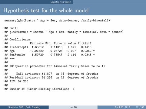
summary(glm(Status ~ Age + Sex, data=donner, family=binomial))
## Call:
## glm(formula = Status ~ Age + Sex, family = binomial, data = donner)
##
## Coefficients:
## Estimate Std. Error z value Pr(>|z|)
## (Intercept) 1.63312 1.11018 1.471 0.1413
## Age -0.07820 0.03728 -2.097 0.0359 *
## SexFemale 1.59729 0.75547 2.114 0.0345 *
## ---
##
## (Dispersion parameter for binomial family taken to be 1)
##
## Null deviance: 61.827 on 44 degrees of freedom
## Residual deviance: 51.256 on 42 degrees of freedom
## AIC: 57.256
##
## Number of Fisher Scoring iterations: 4
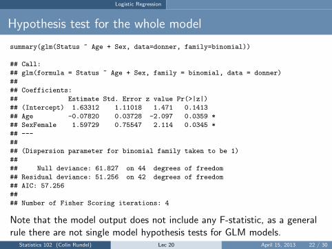
Note that the model output does not include any F-statistic, as a generalrule there are not single model hypothesis tests for GLM models.
Statistics 102 (Colin Rundel) Lec 20 April 15, 2013 22 / 30
Logistic Regression
Hypothesis test for the whole model
summary(glm(Status ~ Age + Sex, data=donner, family=binomial))
## Call:
## glm(formula = Status ~ Age + Sex, family = binomial, data = donner)
##
## Coefficients:
## Estimate Std. Error z value Pr(>|z|)
## (Intercept) 1.63312 1.11018 1.471 0.1413
## Age -0.07820 0.03728 -2.097 0.0359 *
## SexFemale 1.59729 0.75547 2.114 0.0345 *
## ---
##
## (Dispersion parameter for binomial family taken to be 1)
##
## Null deviance: 61.827 on 44 degrees of freedom
## Residual deviance: 51.256 on 42 degrees of freedom
## AIC: 57.256
##
## Number of Fisher Scoring iterations: 4
Note that the model output does not include any F-statistic, as a generalrule there are not single model hypothesis tests for GLM models.
Statistics 102 (Colin Rundel) Lec 20 April 15, 2013 22 / 30
Logistic Regression
Hypothesis tests for a coefficient
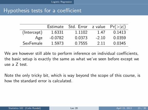
Estimate Std. Error z value Pr(>|z|)(Intercept) 1.6331 1.1102 1.47 0.1413
Age -0.0782 0.0373 -2.10 0.0359SexFemale 1.5973 0.7555 2.11 0.0345
We are however still able to perform inference on individual coefficients,the basic setup is exactly the same as what we’ve seen before except weuse a Z test.
Note the only tricky bit, which is way beyond the scope of this course, ishow the standard error is calculated.
Statistics 102 (Colin Rundel) Lec 20 April 15, 2013 23 / 30
Logistic Regression
Testing for the slope of Age
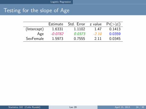
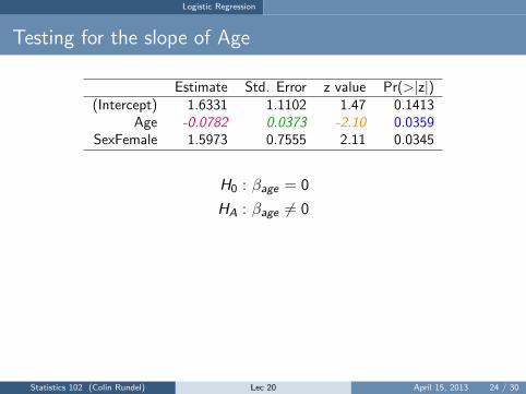
Estimate Std. Error z value Pr(>|z|)(Intercept) 1.6331 1.1102 1.47 0.1413
Age -0.0782 0.0373 -2.10 0.0359SexFemale 1.5973 0.7555 2.11 0.0345
H0 : βage = 0
HA : βage 6= 0
Z =ˆβage − βageSEage
=-0.0782− 0
0.0373= -2.10
p-value = P(|Z | > 2.10) = P(Z > 2.10) + P(Z < -2.10)
= 2× 0.0178 = 0.0359
Statistics 102 (Colin Rundel) Lec 20 April 15, 2013 24 / 30
Logistic Regression
Testing for the slope of Age
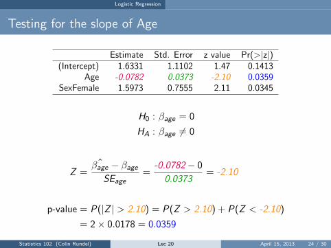
Estimate Std. Error z value Pr(>|z|)(Intercept) 1.6331 1.1102 1.47 0.1413
Age -0.0782 0.0373 -2.10 0.0359SexFemale 1.5973 0.7555 2.11 0.0345
H0 : βage = 0
HA : βage 6= 0
Z =ˆβage − βageSEage
=-0.0782− 0
0.0373= -2.10
p-value = P(|Z | > 2.10) = P(Z > 2.10) + P(Z < -2.10)
= 2× 0.0178 = 0.0359
Statistics 102 (Colin Rundel) Lec 20 April 15, 2013 24 / 30
Logistic Regression
Confidence interval for age slope coefficient
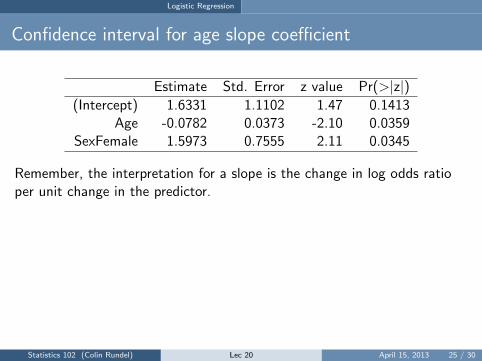
Estimate Std. Error z value Pr(>|z|)(Intercept) 1.6331 1.1102 1.47 0.1413
Age -0.0782 0.0373 -2.10 0.0359SexFemale 1.5973 0.7555 2.11 0.0345
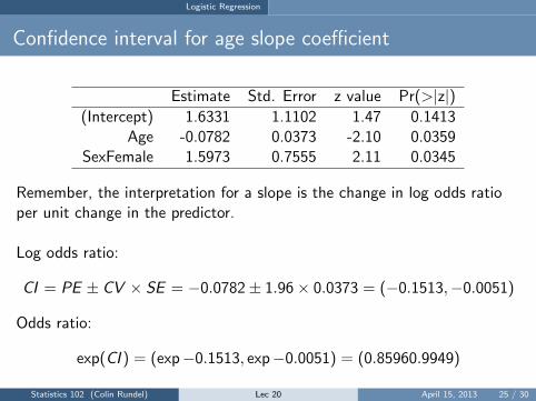
Remember, the interpretation for a slope is the change in log odds ratioper unit change in the predictor.
Log odds ratio:
CI = PE ± CV × SE = −0.0782± 1.96× 0.0373 = (−0.1513,−0.0051)
Odds ratio:
exp(CI ) = (exp−0.1513, exp−0.0051) = (0.85960.9949)
Statistics 102 (Colin Rundel) Lec 20 April 15, 2013 25 / 30
Logistic Regression
Confidence interval for age slope coefficient
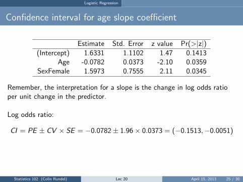
Estimate Std. Error z value Pr(>|z|)(Intercept) 1.6331 1.1102 1.47 0.1413
Age -0.0782 0.0373 -2.10 0.0359SexFemale 1.5973 0.7555 2.11 0.0345
Remember, the interpretation for a slope is the change in log odds ratioper unit change in the predictor.
Log odds ratio:
CI = PE ± CV × SE = −0.0782± 1.96× 0.0373 = (−0.1513,−0.0051)
Odds ratio:
exp(CI ) = (exp−0.1513, exp−0.0051) = (0.85960.9949)
Statistics 102 (Colin Rundel) Lec 20 April 15, 2013 25 / 30
Logistic Regression
Confidence interval for age slope coefficient
Estimate Std. Error z value Pr(>|z|)(Intercept) 1.6331 1.1102 1.47 0.1413
Age -0.0782 0.0373 -2.10 0.0359SexFemale 1.5973 0.7555 2.11 0.0345
Remember, the interpretation for a slope is the change in log odds ratioper unit change in the predictor.
Log odds ratio:
CI = PE ± CV × SE = −0.0782± 1.96× 0.0373 = (−0.1513,−0.0051)
Odds ratio:
exp(CI ) = (exp−0.1513, exp−0.0051) = (0.85960.9949)
Statistics 102 (Colin Rundel) Lec 20 April 15, 2013 25 / 30

Additional Example
1 Background
2 GLMs
3 Logistic Regression
4 Additional Example
Statistics 102
Lec 20 Colin Rundel

Additional Example
Example - Birdkeeping and Lung Cancer
A 1972 - 1981 health survey in The Hague, Netherlands, discovered anassociation between keeping pet birds and increased risk of lung cancer.To investigate birdkeeping as a risk factor, researchers conducted acase-control study of patients in 1985 at four hospitals in The Hague(population 450,000). They identified 49 cases of lung cancer among thepatients who were registered with a general practice, who were age 65 oryounger and who had resided in the city since 1965. They also selected 98controls from a population of residents having the same general agestructure.
From Ramsey, F.L. and Schafer, D.W. (2002). The Statistical Sleuth: A Course in Methods of Data Analysis (2nd ed)
Statistics 102 (Colin Rundel) Lec 20 April 15, 2013 26 / 30
Additional Example
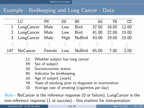
Example - Birdkeeping and Lung Cancer - Data
LC FM SS BK AG YR CD
1 LungCancer Male Low Bird 37.00 19.00 12.002 LungCancer Male Low Bird 41.00 22.00 15.003 LungCancer Male High NoBird 43.00 19.00 15.00...
......
......
......
...147 NoCancer Female Low NoBird 65.00 7.00 2.00
LC Whether subject has lung cancerFM Sex of subjectSS Socioeconomic statusBK Indicator for birdkeepingAG Age of subject (years)YR Years of smoking prior to diagnosis or examinationCD Average rate of smoking (cigarettes per day)
Note - NoCancer is the reference response (0 or failure), LungCancer is thenon-reference response (1 or success) - this matters for interpretation.
Statistics 102 (Colin Rundel) Lec 20 April 15, 2013 27 / 30
Additional Example
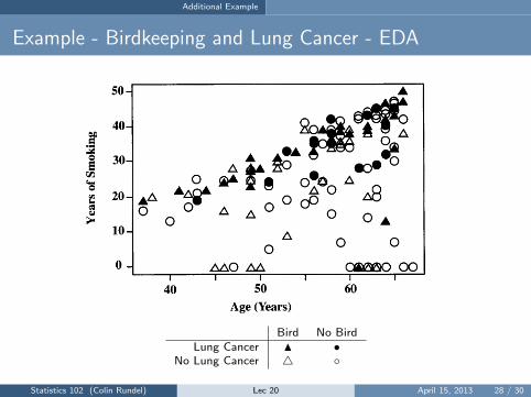
Example - Birdkeeping and Lung Cancer - EDA
Bird No BirdLung Cancer N •
No Lung Cancer 4 ◦
Statistics 102 (Colin Rundel) Lec 20 April 15, 2013 28 / 30
Additional Example
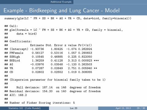
Example - Birdkeeping and Lung Cancer - Modelsummary(glm(LC ~ FM + SS + BK + AG + YR + CD, data=bird, family=binomial))
## Call:
## glm(formula = LC ~ FM + SS + BK + AG + YR + CD, family = binomial,
## data = bird)
##
## Coefficients:
## Estimate Std. Error z value Pr(>|z|)
## (Intercept) -1.93736 1.80425 -1.074 0.282924
## FMFemale 0.56127 0.53116 1.057 0.290653
## SSHigh 0.10545 0.46885 0.225 0.822050
## BKBird 1.36259 0.41128 3.313 0.000923 ***
## AG -0.03976 0.03548 -1.120 0.262503
## YR 0.07287 0.02649 2.751 0.005940 **
## CD 0.02602 0.02552 1.019 0.308055
##
## (Dispersion parameter for binomial family taken to be 1)
##
## Null deviance: 187.14 on 146 degrees of freedom
## Residual deviance: 154.20 on 140 degrees of freedom
## AIC: 168.2
##
## Number of Fisher Scoring iterations: 5
Statistics 102 (Colin Rundel) Lec 20 April 15, 2013 29 / 30
Additional Example
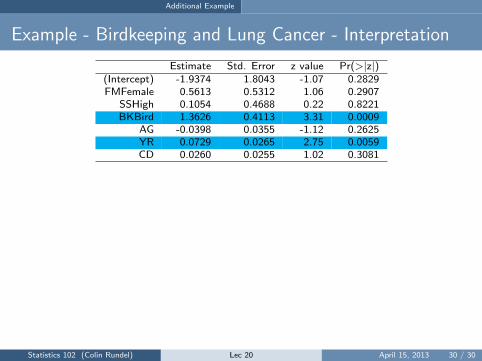
Example - Birdkeeping and Lung Cancer - Interpretation
Estimate Std. Error z value Pr(>|z|)(Intercept) -1.9374 1.8043 -1.07 0.2829FMFemale 0.5613 0.5312 1.06 0.2907
SSHigh 0.1054 0.4688 0.22 0.8221BKBird 1.3626 0.4113 3.31 0.0009
AG -0.0398 0.0355 -1.12 0.2625YR 0.0729 0.0265 2.75 0.0059CD 0.0260 0.0255 1.02 0.3081
Keeping all other predictors constant then,
The odds ratio of getting lung cancer for bird keepers vs non-birdkeepers is exp(1.3626) = 3.91.
The odds ratio of getting lung cancer for an additional year ofsmoking is exp(0.0729) = 1.08.
Statistics 102 (Colin Rundel) Lec 20 April 15, 2013 30 / 30
Additional Example
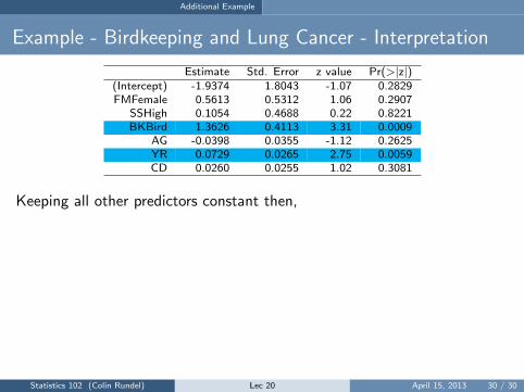
Example - Birdkeeping and Lung Cancer - Interpretation
Estimate Std. Error z value Pr(>|z|)(Intercept) -1.9374 1.8043 -1.07 0.2829FMFemale 0.5613 0.5312 1.06 0.2907
SSHigh 0.1054 0.4688 0.22 0.8221BKBird 1.3626 0.4113 3.31 0.0009
AG -0.0398 0.0355 -1.12 0.2625YR 0.0729 0.0265 2.75 0.0059CD 0.0260 0.0255 1.02 0.3081
Keeping all other predictors constant then,
The odds ratio of getting lung cancer for bird keepers vs non-birdkeepers is exp(1.3626) = 3.91.
The odds ratio of getting lung cancer for an additional year ofsmoking is exp(0.0729) = 1.08.
Statistics 102 (Colin Rundel) Lec 20 April 15, 2013 30 / 30
Additional Example
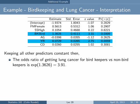
Example - Birdkeeping and Lung Cancer - Interpretation
Estimate Std. Error z value Pr(>|z|)(Intercept) -1.9374 1.8043 -1.07 0.2829FMFemale 0.5613 0.5312 1.06 0.2907
SSHigh 0.1054 0.4688 0.22 0.8221BKBird 1.3626 0.4113 3.31 0.0009
AG -0.0398 0.0355 -1.12 0.2625YR 0.0729 0.0265 2.75 0.0059CD 0.0260 0.0255 1.02 0.3081
Keeping all other predictors constant then,
The odds ratio of getting lung cancer for bird keepers vs non-birdkeepers is exp(1.3626) = 3.91.
The odds ratio of getting lung cancer for an additional year ofsmoking is exp(0.0729) = 1.08.
Statistics 102 (Colin Rundel) Lec 20 April 15, 2013 30 / 30
Additional Example
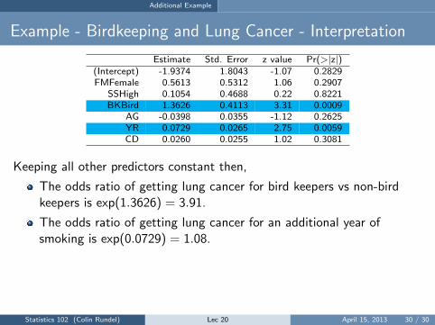
Example - Birdkeeping and Lung Cancer - Interpretation
Estimate Std. Error z value Pr(>|z|)(Intercept) -1.9374 1.8043 -1.07 0.2829FMFemale 0.5613 0.5312 1.06 0.2907
SSHigh 0.1054 0.4688 0.22 0.8221BKBird 1.3626 0.4113 3.31 0.0009
AG -0.0398 0.0355 -1.12 0.2625YR 0.0729 0.0265 2.75 0.0059CD 0.0260 0.0255 1.02 0.3081
Keeping all other predictors constant then,
The odds ratio of getting lung cancer for bird keepers vs non-birdkeepers is exp(1.3626) = 3.91.
The odds ratio of getting lung cancer for an additional year ofsmoking is exp(0.0729) = 1.08.
Statistics 102 (Colin Rundel) Lec 20 April 15, 2013 30 / 30
Related Documents