Lecture 19: Polar and singular value decompositions; generalized eigenspaces; the decomposition theorem (1) Travis Schedler Thurs, Nov 17, 2011 (version: Thurs, Nov 17, 1:00 PM)

Welcome message from author
This document is posted to help you gain knowledge. Please leave a comment to let me know what you think about it! Share it to your friends and learn new things together.
Transcript
Lecture 19: Polar and singular valuedecompositions; generalized eigenspaces; the
decomposition theorem (1)
Travis Schedler
Thurs, Nov 17, 2011 (version: Thurs, Nov 17, 1:00 PM)
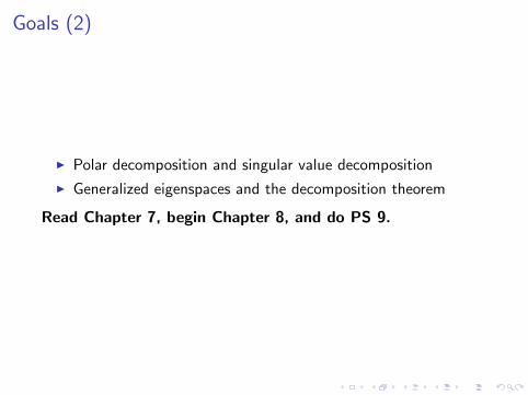
Goals (2)
I Polar decomposition and singular value decomposition
I Generalized eigenspaces and the decomposition theorem
Read Chapter 7, begin Chapter 8, and do PS 9.

Warm-up exercise (3)
(a) Let T be an invertible operator on a f.d. i.p.s. and setP :=
√T ∗T and S := TP−1. Show that S is an isometry.
Recall P is positive, so
T = SP
is a polar decomposition (i.e., S is an isometry and Ppositive).
(b) Now suppose T = 0. Show that polar decompositionsT = SP are exactly
T = S0
for every isometry S , i.e., we have always P = 0 but S can beanything.
One-dimensional analogue: Either z ∈ C is invertible, in which casez = (z/|z |)|z | = sp or else z is zero, in which case z = s · 0 for anys of absolute value one.
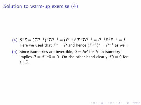
Solution to warm-up exercise (4)
(a) S∗S = (TP−1)∗TP−1 = (P−1)∗T ∗TP−1 = P−1P2P−1 = I .Here we used that P∗ = P and hence (P−1)∗ = P−1 as well.
(b) Since isometries are invertible, 0 = SP for S an isometryimplies P = S−10 = 0. On the other hand clearly S0 = 0 forall S .
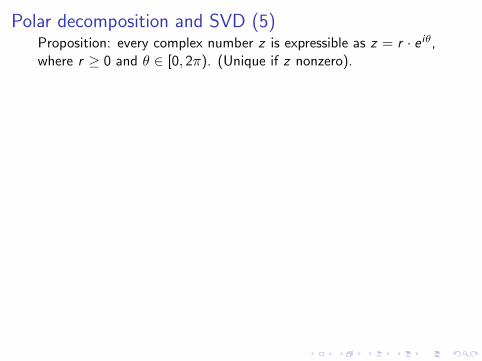
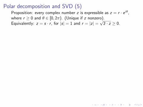
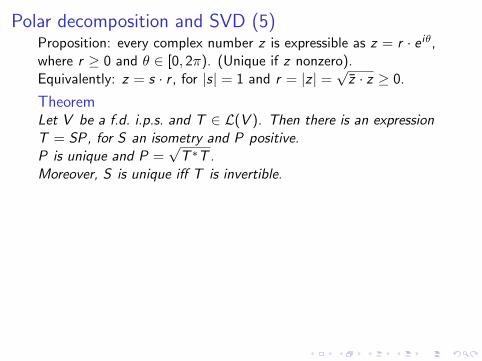
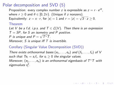
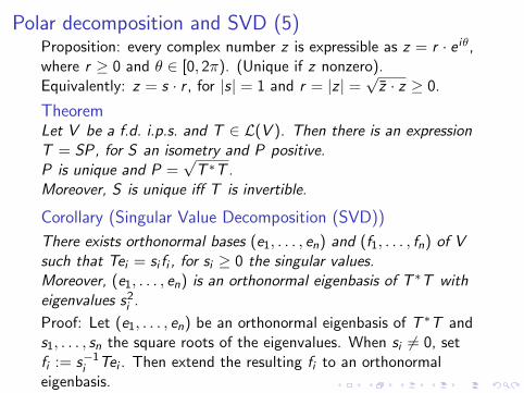
Polar decomposition and SVD (5)Proposition: every complex number z is expressible as z = r · e iθ,where r ≥ 0 and θ ∈ [0, 2π). (Unique if z nonzero).
Equivalently: z = s · r , for |s| = 1 and r = |z | =√
z · z ≥ 0.
TheoremLet V be a f.d. i.p.s. and T ∈ L(V ). Then there is an expressionT = SP, for S an isometry and P positive.P is unique and P =
√T ∗T .
Moreover, S is unique iff T is invertible.
Corollary (Singular Value Decomposition (SVD))
There exists orthonormal bases (e1, . . . , en) and (f1, . . . , fn) of Vsuch that Tei = si fi , for si ≥ 0 the singular values.Moreover, (e1, . . . , en) is an orthonormal eigenbasis of T ∗T witheigenvalues s2i .
Proof: Let (e1, . . . , en) be an orthonormal eigenbasis of T ∗T ands1, . . . , sn the square roots of the eigenvalues. When si 6= 0, setfi := s−1i Tei . Then extend the resulting fi to an orthonormaleigenbasis.
Polar decomposition and SVD (5)Proposition: every complex number z is expressible as z = r · e iθ,where r ≥ 0 and θ ∈ [0, 2π). (Unique if z nonzero).Equivalently: z = s · r , for |s| = 1 and r = |z | =
√z · z ≥ 0.
TheoremLet V be a f.d. i.p.s. and T ∈ L(V ). Then there is an expressionT = SP, for S an isometry and P positive.P is unique and P =
√T ∗T .
Moreover, S is unique iff T is invertible.
Corollary (Singular Value Decomposition (SVD))
There exists orthonormal bases (e1, . . . , en) and (f1, . . . , fn) of Vsuch that Tei = si fi , for si ≥ 0 the singular values.Moreover, (e1, . . . , en) is an orthonormal eigenbasis of T ∗T witheigenvalues s2i .
Proof: Let (e1, . . . , en) be an orthonormal eigenbasis of T ∗T ands1, . . . , sn the square roots of the eigenvalues. When si 6= 0, setfi := s−1i Tei . Then extend the resulting fi to an orthonormaleigenbasis.

Uniqueness of polar decomposition (6)
I If T = SP, then T ∗T = P∗S∗SP = P∗P = P2, soP =
√T ∗T . Thus P is unique (positive operators have unique
positive square roots; see the slides for Lecture 18 or Axler).
I If T is invertible, S = TP−1 so S is unique.
I Conversely, if T is not invertible, neither is P, and we canreplace S by SS ′ where S ′ is an isometry such that S ′v = vfor all eigenvectors v of nonzero eigenvalue. So then S is notunique.
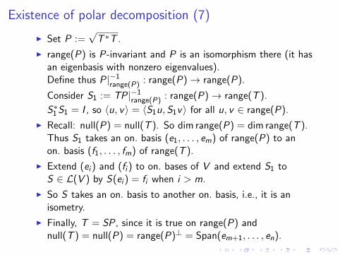
Existence of polar decomposition (7)
I Set P :=√
T ∗T .
I range(P) is P-invariant and P is an isomorphism there (it hasan eigenbasis with nonzero eigenvalues).Define thus P|−1range(P) : range(P)→ range(P).
Consider S1 := TP|−1range(P) : range(P)→ range(T ).
S∗1S1 = I , so 〈u, v〉 = 〈S1u, S1v〉 for all u, v ∈ range(P).
I Recall: null(P) = null(T ). So dim range(P) = dim range(T ).Thus S1 takes an on. basis (e1, . . . , em) of range(P) to anon. basis (f1, . . . , fm) of range(T ).
I Extend (ei ) and (fi ) to on. bases of V and extend S1 toS ∈ L(V ) by S(ei ) = fi when i > m.
I So S takes an on. basis to another on. basis, i.e., it is anisometry.
I Finally, T = SP, since it is true on range(P) andnull(T ) = null(P) = range(P)⊥ = Span(em+1, . . . , en).

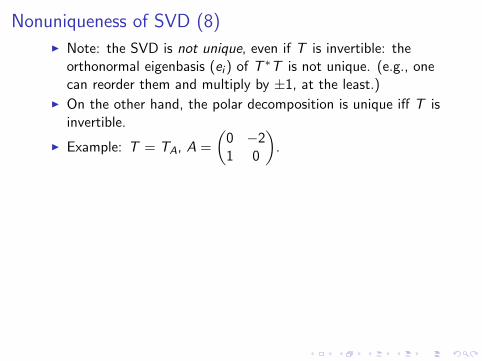
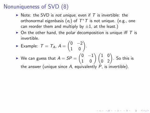
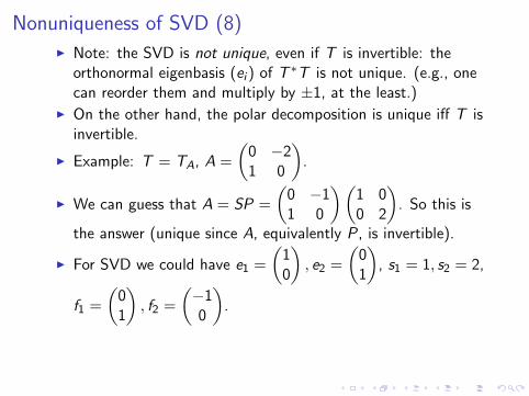
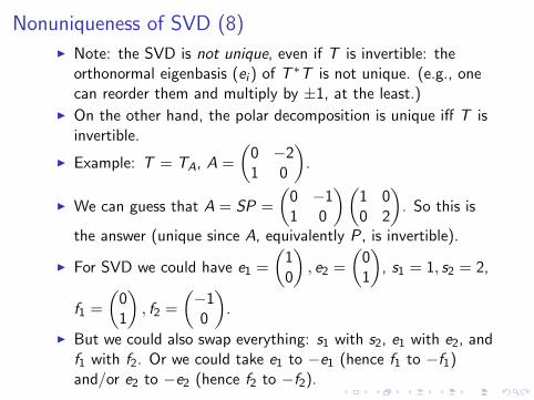
Nonuniqueness of SVD (8)
I Note: the SVD is not unique, even if T is invertible: theorthonormal eigenbasis (ei ) of T ∗T is not unique. (e.g., onecan reorder them and multiply by ±1, at the least.)
I On the other hand, the polar decomposition is unique iff T isinvertible.
I Example: T = TA, A =
(0 −21 0
).
I We can guess that A = SP =
(0 −11 0
)(1 00 2
). So this is
the answer (unique since A, equivalently P, is invertible).
I For SVD we could have e1 =
(10
), e2 =
(01
), s1 = 1, s2 = 2,
f1 =
(01
), f2 =
(−10
).
I But we could also swap everything: s1 with s2, e1 with e2, andf1 with f2. Or we could take e1 to −e1 (hence f1 to −f1)and/or e2 to −e2 (hence f2 to −f2).
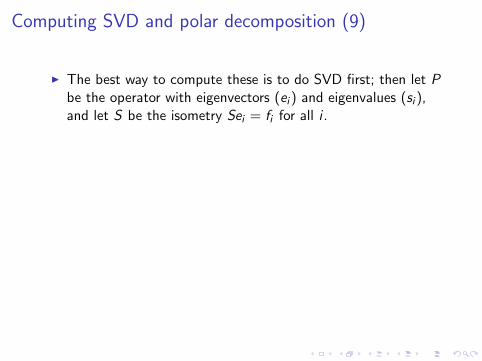
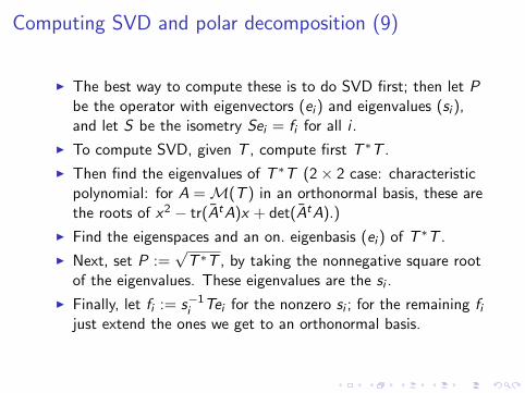
Computing SVD and polar decomposition (9)
I The best way to compute these is to do SVD first; then let Pbe the operator with eigenvectors (ei ) and eigenvalues (si ),and let S be the isometry Sei = fi for all i .
I To compute SVD, given T , compute first T ∗T .
I Then find the eigenvalues of T ∗T (2× 2 case: characteristicpolynomial: for A =M(T ) in an orthonormal basis, these arethe roots of x2 − tr(AtA)x + det(AtA).)
I Find the eigenspaces and an on. eigenbasis (ei ) of T ∗T .
I Next, set P :=√
T ∗T , by taking the nonnegative square rootof the eigenvalues. These eigenvalues are the si .
I Finally, let fi := s−1i Tei for the nonzero si ; for the remaining fijust extend the ones we get to an orthonormal basis.
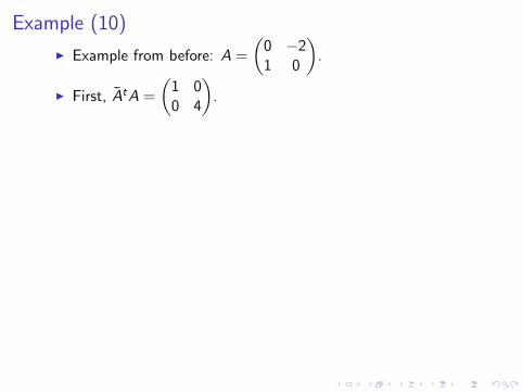
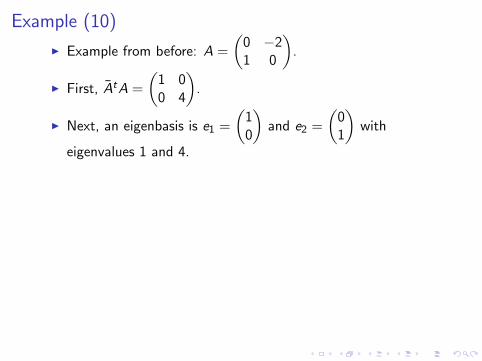
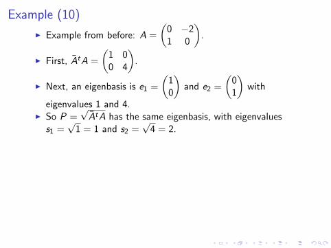
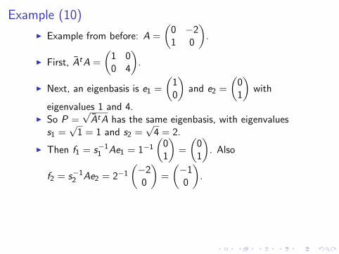
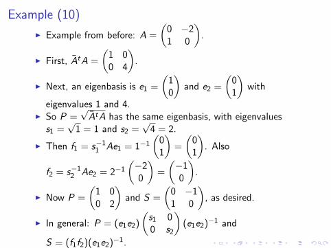
Example (10)
I Example from before: A =
(0 −21 0
).
I First, AtA =
(1 00 4
).
I Next, an eigenbasis is e1 =
(10
)and e2 =
(01
)with
eigenvalues 1 and 4.I So P =
√AtA has the same eigenbasis, with eigenvalues
s1 =√
1 = 1 and s2 =√
4 = 2.
I Then f1 = s−11 Ae1 = 1−1(
01
)=
(01
). Also
f2 = s−12 Ae2 = 2−1(−20
)=
(−10
).
I Now P =
(1 00 2
)and S =
(0 −11 0
), as desired.
I In general: P = (e1e2)
(s1 00 s2
)(e1e2)−1 and
S = (f1f2)(e1e2)−1.
Example (10)
I Example from before: A =
(0 −21 0
).
I First, AtA =
(1 00 4
).
I Next, an eigenbasis is e1 =
(10
)and e2 =
(01
)with
eigenvalues 1 and 4.
I So P =√
AtA has the same eigenbasis, with eigenvaluess1 =
√1 = 1 and s2 =
√4 = 2.
I Then f1 = s−11 Ae1 = 1−1(
01
)=
(01
). Also
f2 = s−12 Ae2 = 2−1(−20
)=
(−10
).
I Now P =
(1 00 2
)and S =
(0 −11 0
), as desired.
I In general: P = (e1e2)
(s1 00 s2
)(e1e2)−1 and
S = (f1f2)(e1e2)−1.
Example (10)
I Example from before: A =
(0 −21 0
).
I First, AtA =
(1 00 4
).
I Next, an eigenbasis is e1 =
(10
)and e2 =
(01
)with
eigenvalues 1 and 4.I So P =
√AtA has the same eigenbasis, with eigenvalues
s1 =√
1 = 1 and s2 =√
4 = 2.
I Then f1 = s−11 Ae1 = 1−1(
01
)=
(01
). Also
f2 = s−12 Ae2 = 2−1(−20
)=
(−10
).
I Now P =
(1 00 2
)and S =
(0 −11 0
), as desired.
I In general: P = (e1e2)
(s1 00 s2
)(e1e2)−1 and
S = (f1f2)(e1e2)−1.
Example (10)
I Example from before: A =
(0 −21 0
).
I First, AtA =
(1 00 4
).
I Next, an eigenbasis is e1 =
(10
)and e2 =
(01
)with
eigenvalues 1 and 4.I So P =
√AtA has the same eigenbasis, with eigenvalues
s1 =√
1 = 1 and s2 =√
4 = 2.
I Then f1 = s−11 Ae1 = 1−1(
01
)=
(01
). Also
f2 = s−12 Ae2 = 2−1(−20
)=
(−10
).
I Now P =
(1 00 2
)and S =
(0 −11 0
), as desired.
I In general: P = (e1e2)
(s1 00 s2
)(e1e2)−1 and
S = (f1f2)(e1e2)−1.
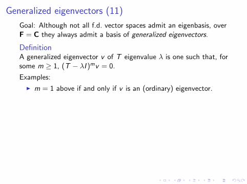
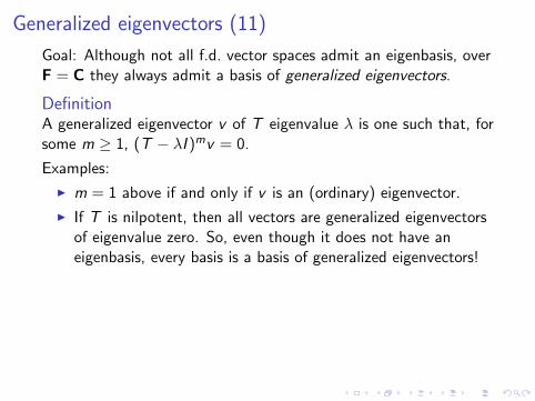
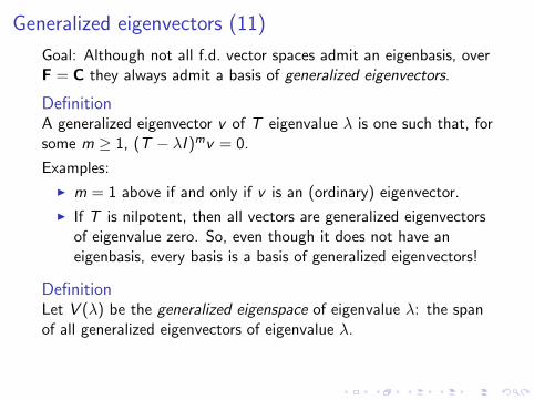
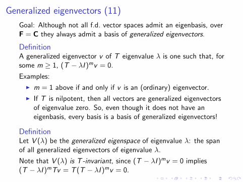
Generalized eigenvectors (11)
Goal: Although not all f.d. vector spaces admit an eigenbasis, overF = C they always admit a basis of generalized eigenvectors.
DefinitionA generalized eigenvector v of T eigenvalue λ is one such that, forsome m ≥ 1, (T − λI )mv = 0.
Examples:
I m = 1 above if and only if v is an (ordinary) eigenvector.
I If T is nilpotent, then all vectors are generalized eigenvectorsof eigenvalue zero. So, even though it does not have aneigenbasis, every basis is a basis of generalized eigenvectors!
DefinitionLet V (λ) be the generalized eigenspace of eigenvalue λ: the spanof all generalized eigenvectors of eigenvalue λ.
Note that V (λ) is T -invariant, since (T − λI )mv = 0 implies(T − λI )mTv = T (T − λI )mv = 0.
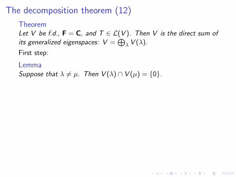
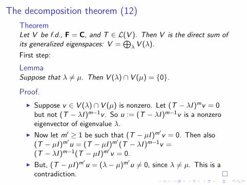
The decomposition theorem (12)
TheoremLet V be f.d., F = C, and T ∈ L(V ). Then V is the direct sum ofits generalized eigenspaces: V =
⊕λ V (λ).
First step:
LemmaSuppose that λ 6= µ. Then V (λ) ∩ V (µ) = {0}.
Proof.
I Suppose v ∈ V (λ) ∩ V (µ) is nonzero. Let (T − λI )mv = 0but not (T − λI )m−1v . So u := (T − λI )m−1v is a nonzeroeigenvector of eigenvalue λ.
I Now let m′ ≥ 1 be such that (T − µI )m′v = 0. Then also
(T − µI )m′u = (T − µI )m
′(T − λI )m−1v =
(T − λI )m−1(T − µI )m′v = 0.
I But, (T − µI )m′u = (λ− µ)m
′u 6= 0, since λ 6= µ. This is a
contradiction.
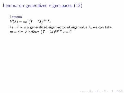
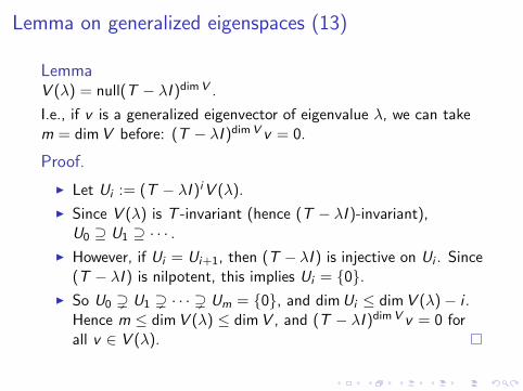
Lemma on generalized eigenspaces (13)
LemmaV (λ) = null(T − λI )dimV .
I.e., if v is a generalized eigenvector of eigenvalue λ, we can takem = dim V before: (T − λI )dimV v = 0.
Proof.
I Let Ui := (T − λI )iV (λ).
I Since V (λ) is T -invariant (hence (T − λI )-invariant),U0 ⊇ U1 ⊇ · · · .
I However, if Ui = Ui+1, then (T − λI ) is injective on Ui . Since(T − λI ) is nilpotent, this implies Ui = {0}.
I So U0 ) U1 ) · · · ) Um = {0}, and dim Ui ≤ dim V (λ)− i .Hence m ≤ dim V (λ) ≤ dim V , and (T − λI )dimV v = 0 forall v ∈ V (λ).
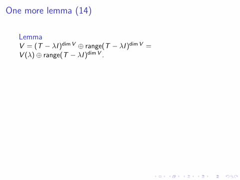
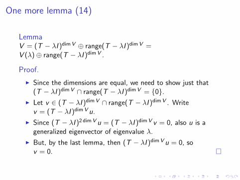
One more lemma (14)
LemmaV = (T − λI )dimV ⊕ range(T − λI )dimV =V (λ)⊕ range(T − λI )dimV .
Proof.
I Since the dimensions are equal, we need to show just that(T − λI )dimV ∩ range(T − λI )dimV = {0}.
I Let v ∈ (T − λI )dimV ∩ range(T − λI )dimV . Writev = (T − λI )dimV u.
I Since (T − λI )2 dimV u = (T − λI )dimV v = 0, also u is ageneralized eigenvector of eigenvalue λ.
I But, by the last lemma, then (T − λI )dimV u = 0, sov = 0.
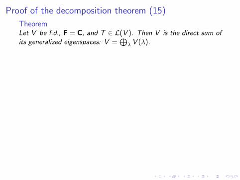
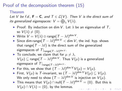
Proof of the decomposition theorem (15)
TheoremLet V be f.d., F = C, and T ∈ L(V ). Then V is the direct sum ofits generalized eigenspaces: V =
⊕λ V (λ).
I Proof: By induction on dim V . Let λ be an eigenvalue of T ,so V (λ) 6= {0}.
I Write V = V (λ)⊕ range(T − λI )dimV .I Since dim range(T − λI )dimV < dim V , the ind. hyp. shows
that range(T − λI ) is the direct sum of the generalizedeigenspaces of T |range(T−λI )dim V .
I To conclude, we claim that for µ 6= λ,V (µ) ⊆ range(T − λI )dimV . Thus V (µ) is a generalizedeigenspace of T |range(T−λI )dim V .
I For this, we show that (T − λI )dimV V (µ) = V (µ).I First, V (µ) is T -invariant, so (T − λI )dimV V (µ) ⊆ V (µ).
We only need to show (T − λI )dimV is injective on V (µ).I This means that V (µ) ∩ null(T − λI )dimV = {0}. But this is
V (µ) ∩ V (λ) = {0}, by the lemmas.
Related Documents