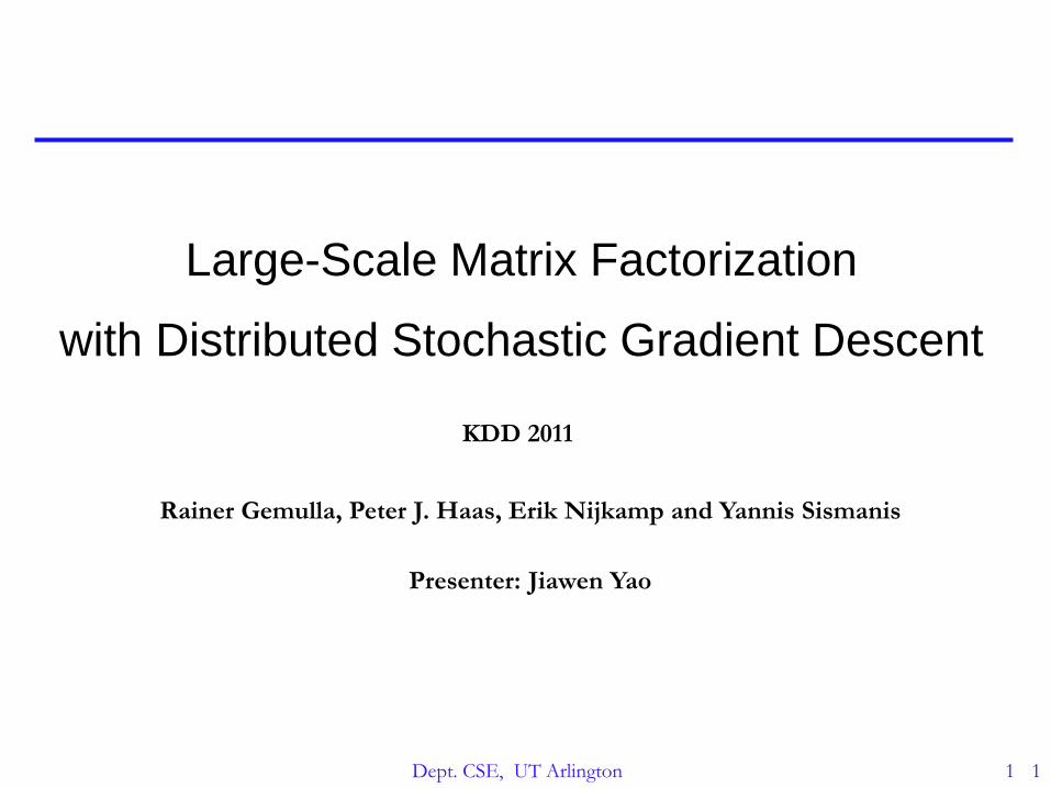
Dept. CSE, UT Arlington 1 1 Large-Scale Matrix Factorization with Distributed Stochastic Gradient Descent KDD 2011 Rainer Gemulla, Peter J. Haas, Erik Nijkamp and Yannis Sismanis Presenter: Jiawen Yao

Welcome message from author
This document is posted to help you gain knowledge. Please leave a comment to let me know what you think about it! Share it to your friends and learn new things together.
Transcript
Dept. CSE, UT Arlington 1 1
Large-Scale Matrix Factorization
with Distributed Stochastic Gradient Descent
KDD 2011
Rainer Gemulla, Peter J. Haas, Erik Nijkamp and Yannis Sismanis
Presenter: Jiawen Yao
Dept. CSE, UT Arlington 2
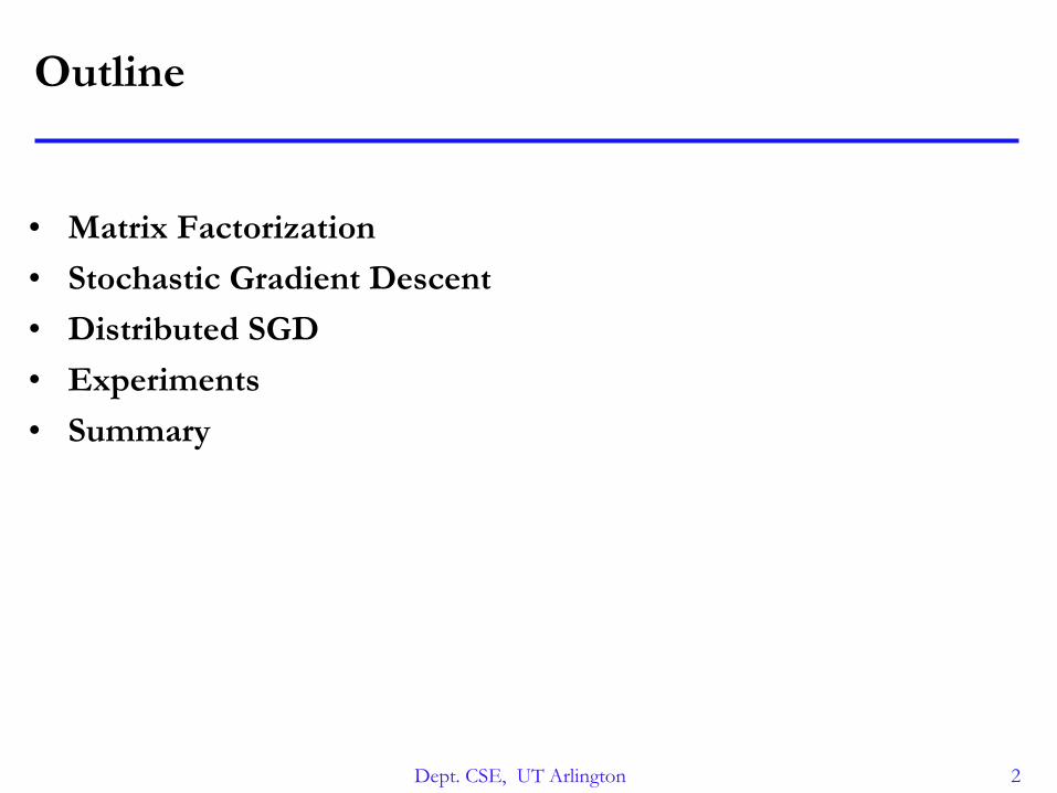
Outline
• Matrix Factorization
• Stochastic Gradient Descent
• Distributed SGD
• Experiments
• Summary
Dept. CSE, UT Arlington 3
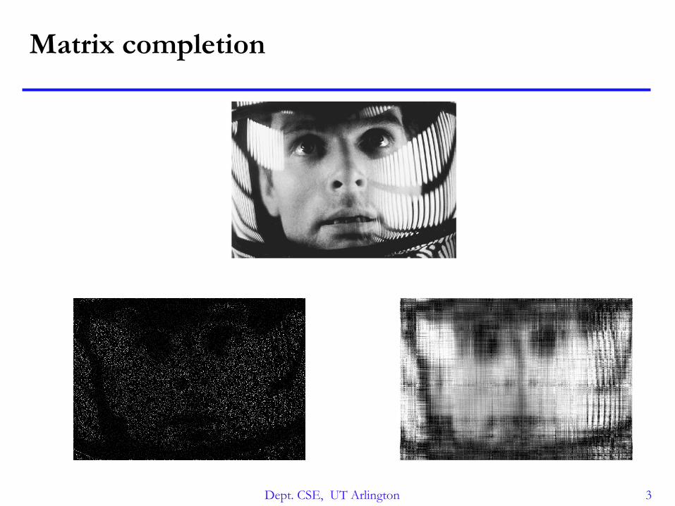
Matrix completion
Dept. CSE, UT Arlington 4
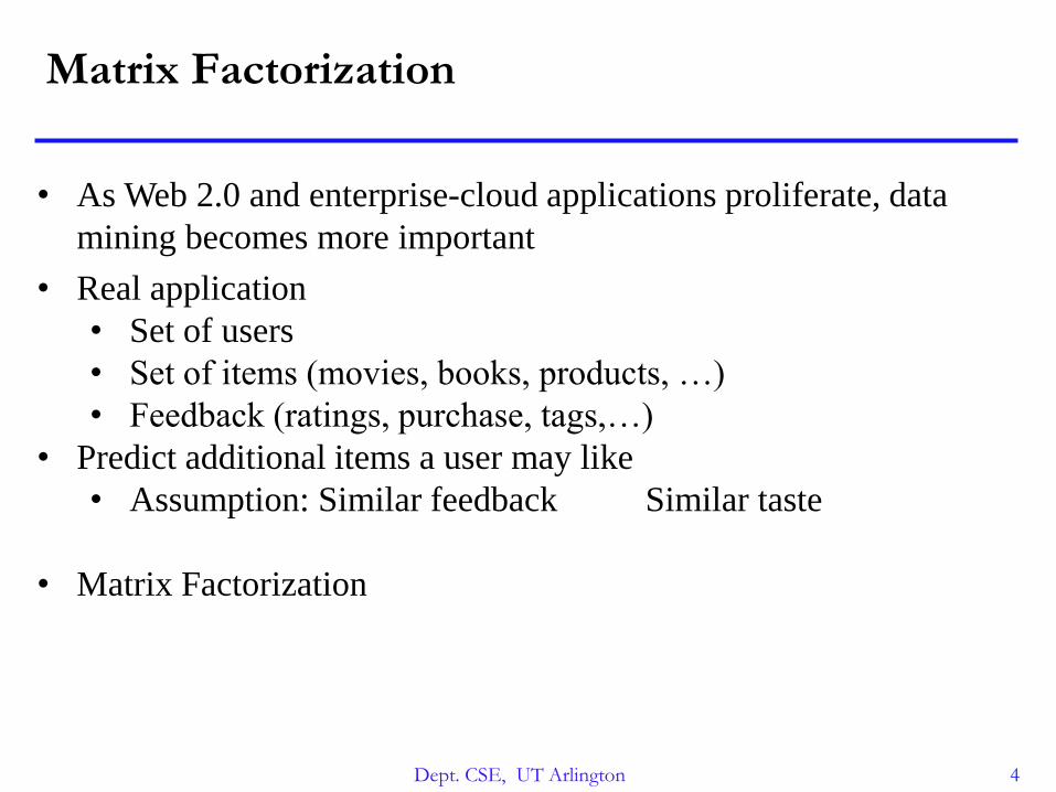
Matrix Factorization
• Real application
• Set of users
• Set of items (movies, books, products, …)
• Feedback (ratings, purchase, tags,…)
• Predict additional items a user may like
• Assumption: Similar feedback Similar taste
• Matrix Factorization
• As Web 2.0 and enterprise-cloud applications proliferate, data
mining becomes more important
Dept. CSE, UT Arlington 5
Matrix Factorization
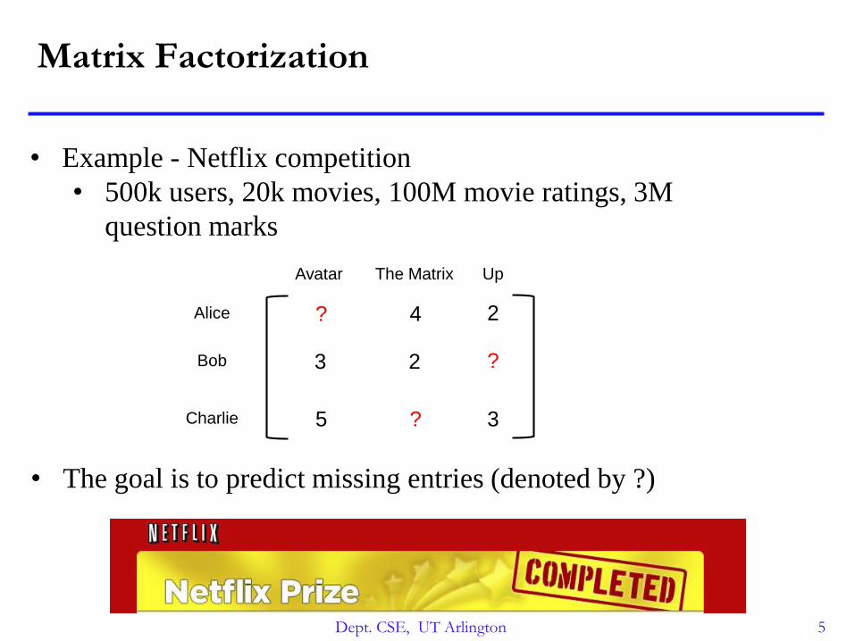
• Example - Netflix competition
• 500k users, 20k movies, 100M movie ratings, 3M
question marks
Avatar The Matrix Up
Alice
Bob
Charlie
?
3
5
4
2
?
2
?
3
• The goal is to predict missing entries (denoted by ?)
Dept. CSE, UT Arlington 6
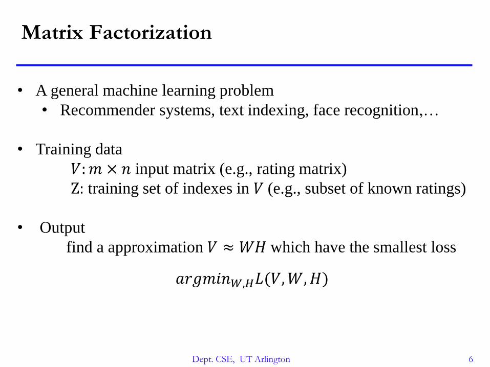
• A general machine learning problem
• Recommender systems, text indexing, face recognition,…
• Training data
𝑉:𝑚 × 𝑛 input matrix (e.g., rating matrix)
Z: training set of indexes in 𝑉 (e.g., subset of known ratings)
• Output
find a approximation 𝑉 ≈ 𝑊𝐻 which have the smallest loss
𝑎𝑟𝑔𝑚𝑖𝑛𝑊,𝐻𝐿(𝑉,𝑊,𝐻)
Matrix Factorization
Dept. CSE, UT Arlington 7
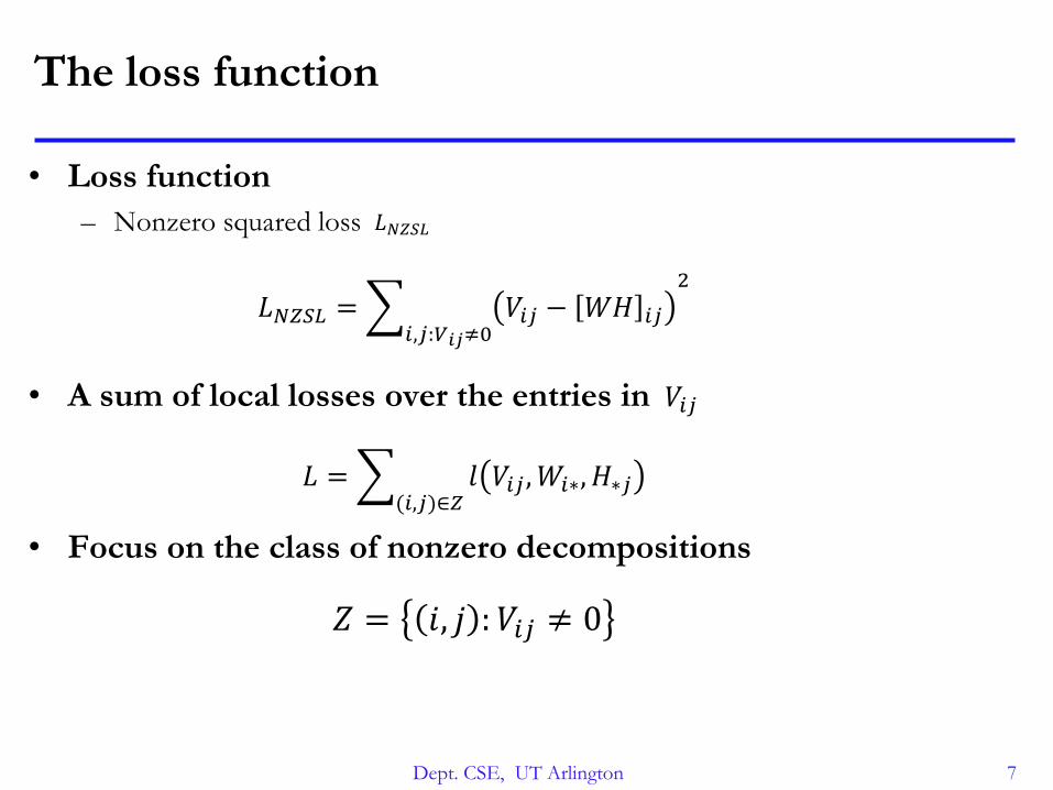
The loss function
• Loss function
– Nonzero squared loss
• A sum of local losses over the entries in
• Focus on the class of nonzero decompositions
𝐿𝑁𝑍𝑆𝐿
𝐿𝑁𝑍𝑆𝐿 = 𝑖,𝑗:𝑉𝑖𝑗≠0
𝑉𝑖𝑗 − 𝑊𝐻 𝑖𝑗
2
𝑉𝑖𝑗
𝐿 = (𝑖,𝑗)∈𝑍
𝑙 𝑉𝑖𝑗 ,𝑊𝑖∗, 𝐻∗𝑗
𝑍 = 𝑖, 𝑗 : 𝑉𝑖𝑗 ≠ 0
Dept. CSE, UT Arlington 8
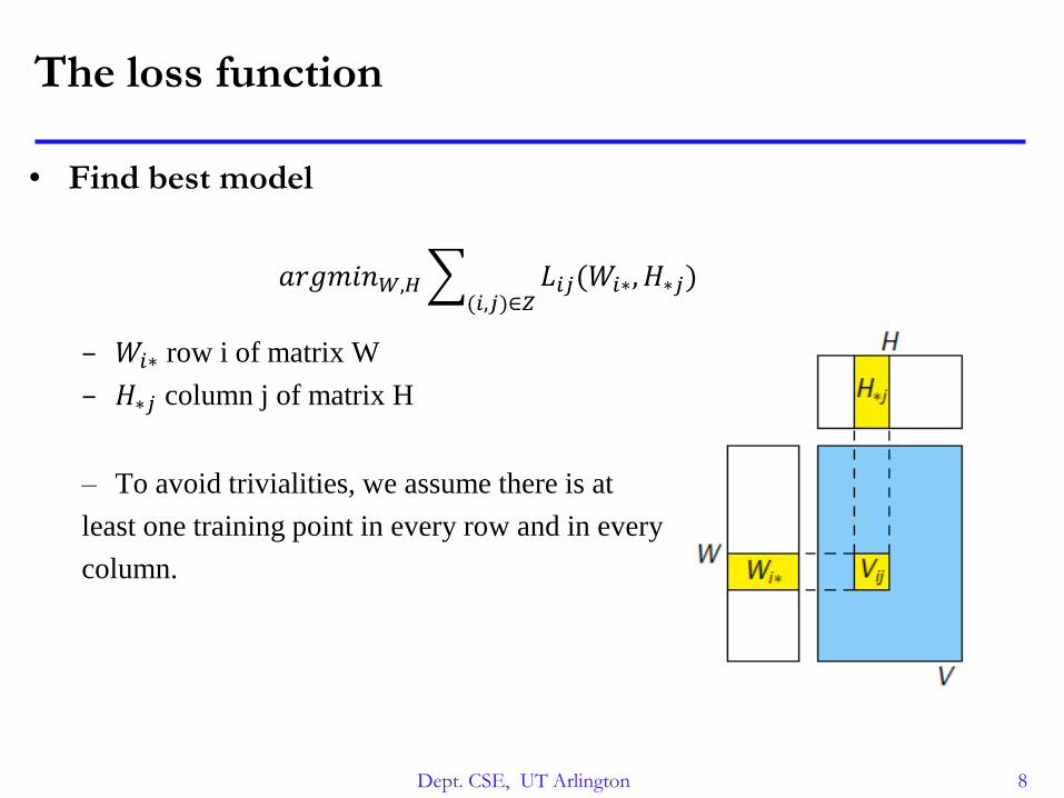
• Find best model
– 𝑊𝑖∗ row i of matrix W
– 𝐻∗𝑗 column j of matrix H
– To avoid trivialities, we assume there is at
least one training point in every row and in every
column.
𝑎𝑟𝑔𝑚𝑖𝑛𝑊,𝐻 (𝑖,𝑗)∈𝑍
𝐿𝑖𝑗(𝑊𝑖∗, 𝐻∗𝑗)
The loss function
Dept. CSE, UT Arlington 9
Prior Work
• Specialized algorithms
– Designed for a small class of loss functions
– GKL loss
• Generic algorithms
– Handle all differentiable loss functions that decompose into summation form
– Distributed gradient descent (DGD), Partitioned SGD (PSGD)
– The proposed
Dept. CSE, UT Arlington 10
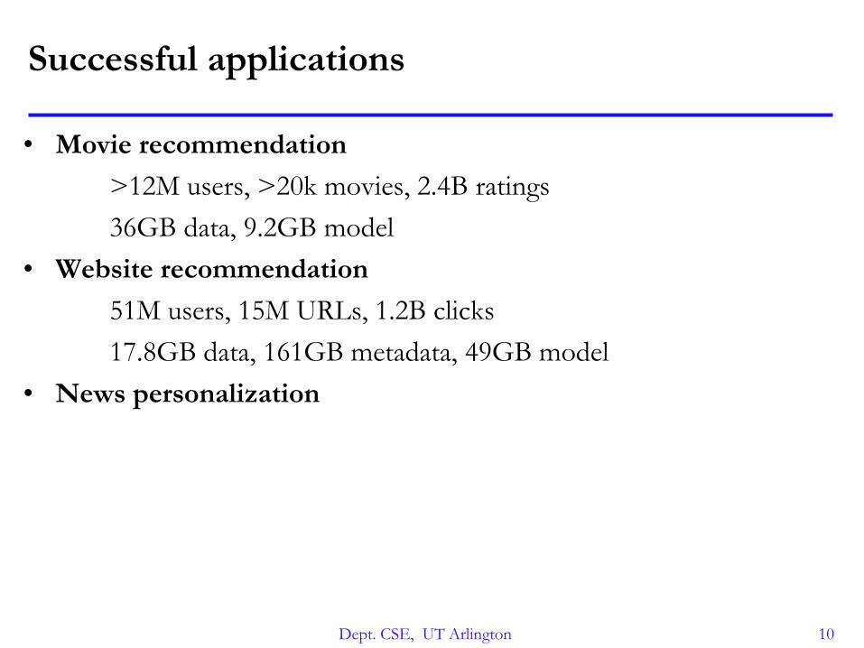
Successful applications
• Movie recommendation
>12M users, >20k movies, 2.4B ratings
36GB data, 9.2GB model
• Website recommendation
51M users, 15M URLs, 1.2B clicks
17.8GB data, 161GB metadata, 49GB model
• News personalization
Dept. CSE, UT Arlington 11
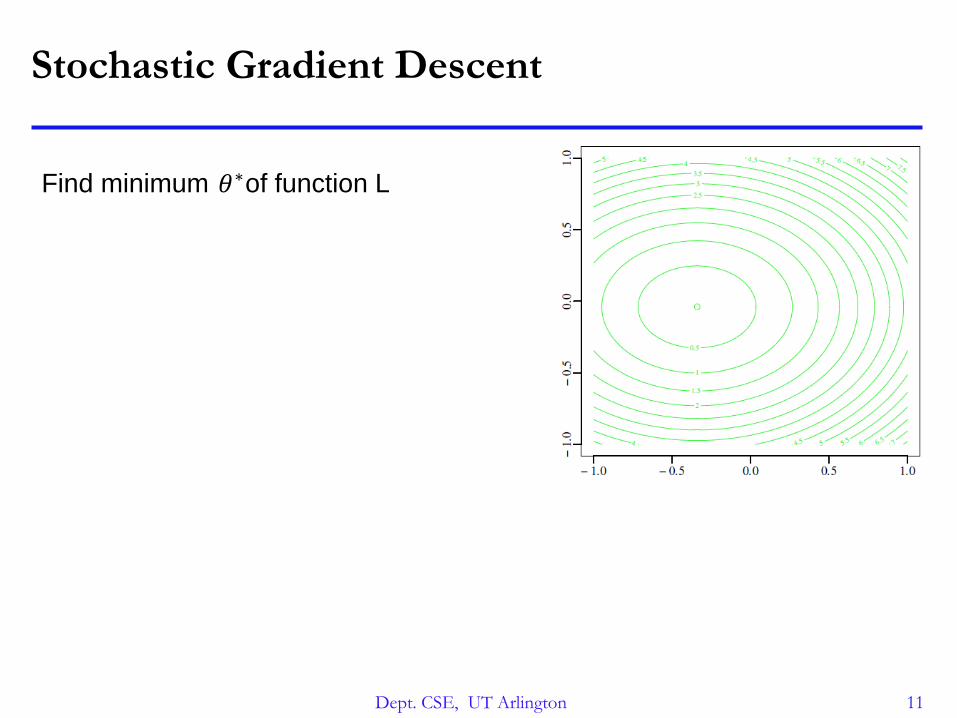
Stochastic Gradient Descent
Find minimum of function L𝜃∗
Dept. CSE, UT Arlington 12
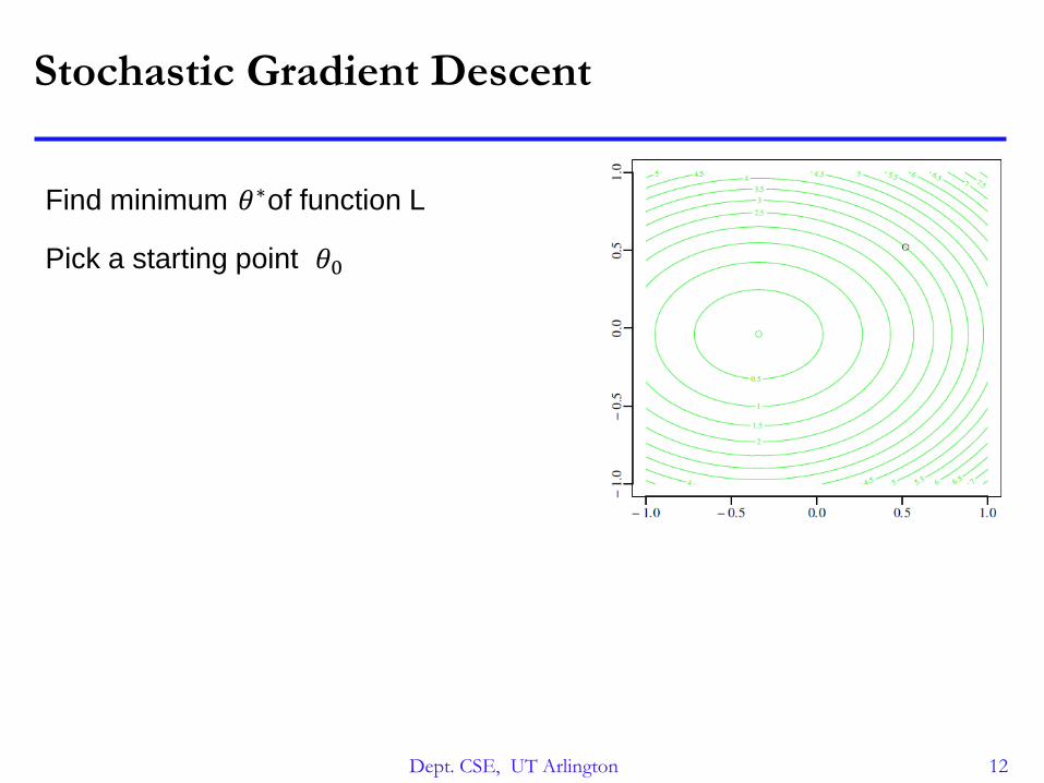
Stochastic Gradient Descent
Find minimum of function L𝜃∗
Pick a starting point 𝜃0
Dept. CSE, UT Arlington 13
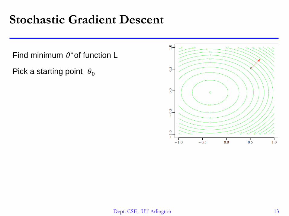
Stochastic Gradient Descent
Find minimum of function L𝜃∗
Pick a starting point 𝜃0
Dept. CSE, UT Arlington 14
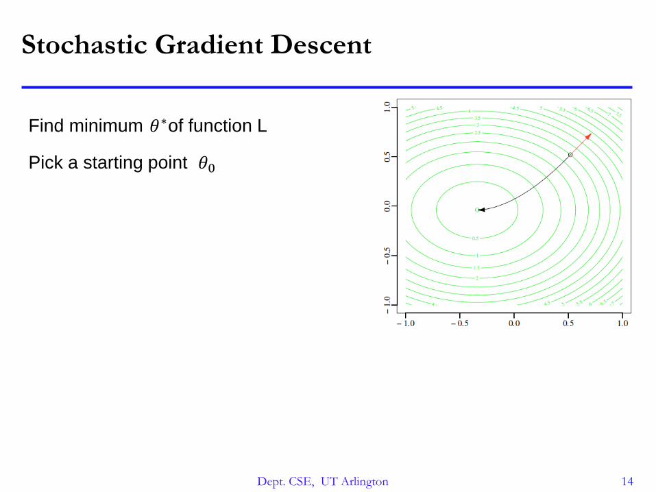
Stochastic Gradient Descent
Find minimum of function L𝜃∗
Pick a starting point 𝜃0
Dept. CSE, UT Arlington 15
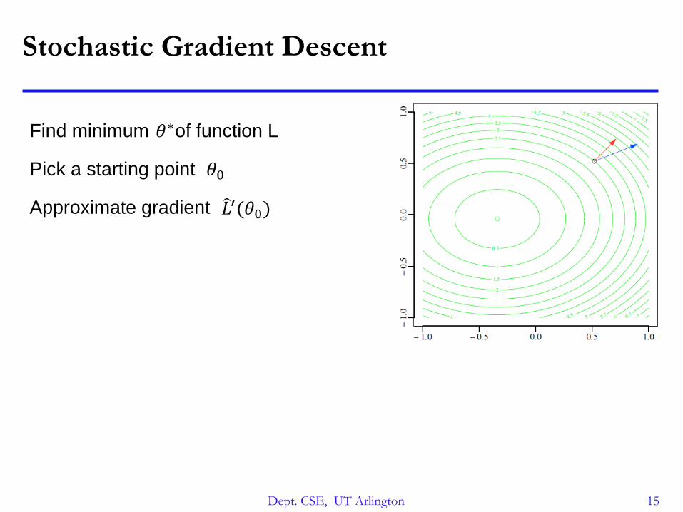
Stochastic Gradient Descent
Find minimum of function L𝜃∗
Pick a starting point 𝜃0
Approximate gradient 𝐿′(𝜃0)
Dept. CSE, UT Arlington 16
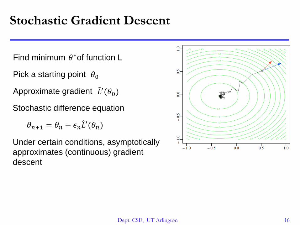
Stochastic Gradient Descent
Find minimum of function L𝜃∗
Pick a starting point 𝜃0
Approximate gradient 𝐿′(𝜃0)
Stochastic difference equation
𝜃𝑛+1 = 𝜃𝑛 − 𝜖𝑛 𝐿′(𝜃𝑛)
Under certain conditions, asymptotically
approximates (continuous) gradient
descent
Dept. CSE, UT Arlington 17
Stochastic Gradient Descent for Matrix Factorization
Set and use 𝜃 = (𝑊,𝐻)
Where N = 𝑍 and training point z is chosen randomly from the training set.
𝐿(𝜃) = (𝑖,𝑗)∈𝑍
𝐿𝑖𝑗 𝑊𝑖∗, 𝐻∗𝑗
𝐿′(𝜃) = (𝑖,𝑗)∈𝑍
𝐿𝑖𝑗′ 𝑊𝑖∗, 𝐻∗𝑗
𝐿′(𝜃, 𝑧) = 𝑁𝐿𝑧′ (𝑊𝑖𝑧∗, 𝐻∗𝑗𝑧)
𝑍 = 𝑖, 𝑗 : 𝑉𝑖𝑗 ≠ 0
Dept. CSE, UT Arlington 18
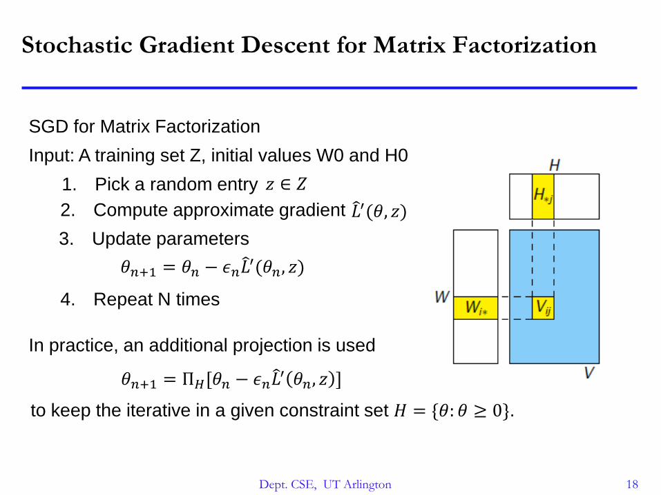
Stochastic Gradient Descent for Matrix Factorization
SGD for Matrix Factorization
𝜃𝑛+1 = 𝜃𝑛 − 𝜖𝑛 𝐿′(𝜃𝑛, 𝑧)
Input: A training set Z, initial values W0 and H0
1. Pick a random entry 𝑧 ∈ 𝑍
2. Compute approximate gradient 𝐿′(𝜃, 𝑧)
3. Update parameters
4. Repeat N times
𝜃𝑛+1 = Π𝐻[𝜃𝑛 − 𝜖𝑛 𝐿′ 𝜃𝑛, 𝑧 ]
In practice, an additional projection is used
to keep the iterative in a given constraint set 𝐻 = {𝜃: 𝜃 ≥ 0}.
Dept. CSE, UT Arlington 19
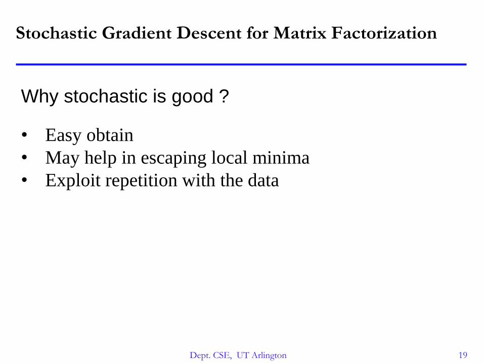
Stochastic Gradient Descent for Matrix Factorization
Why stochastic is good ?
• Easy obtain
• May help in escaping local minima
• Exploit repetition with the data
Dept. CSE, UT Arlington 20
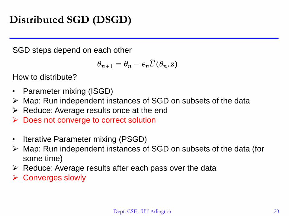
Distributed SGD (DSGD)
SGD steps depend on each other
How to distribute?
• Parameter mixing (ISGD)
Map: Run independent instances of SGD on subsets of the data
Reduce: Average results once at the end
Does not converge to correct solution
• Iterative Parameter mixing (PSGD)
Map: Run independent instances of SGD on subsets of the data (for
some time)
Reduce: Average results after each pass over the data
Converges slowly
𝜃𝑛+1 = 𝜃𝑛 − 𝜖𝑛 𝐿′(𝜃𝑛, 𝑧)
Dept. CSE, UT Arlington 21
Distributed SGD (DSGD)
Dept. CSE, UT Arlington 22
Stratified SGD
Proposed Stratified SGD to obtain an efficient DSGD for matrix factorization
𝐿 𝜃 = 𝜔1𝐿1 𝜃 + 𝜔2𝐿2 𝜃 + ⋯+ 𝜔𝑞𝐿𝑞 𝜃
The sum of loss function 𝐿𝑠, and 𝑠 is a stratum.
A stratum is a part or partition of dataset
SSGD runs standard SGD on a single stratum at a time, but switches
strata in a way that guarantees correctness
Dept. CSE, UT Arlington 23
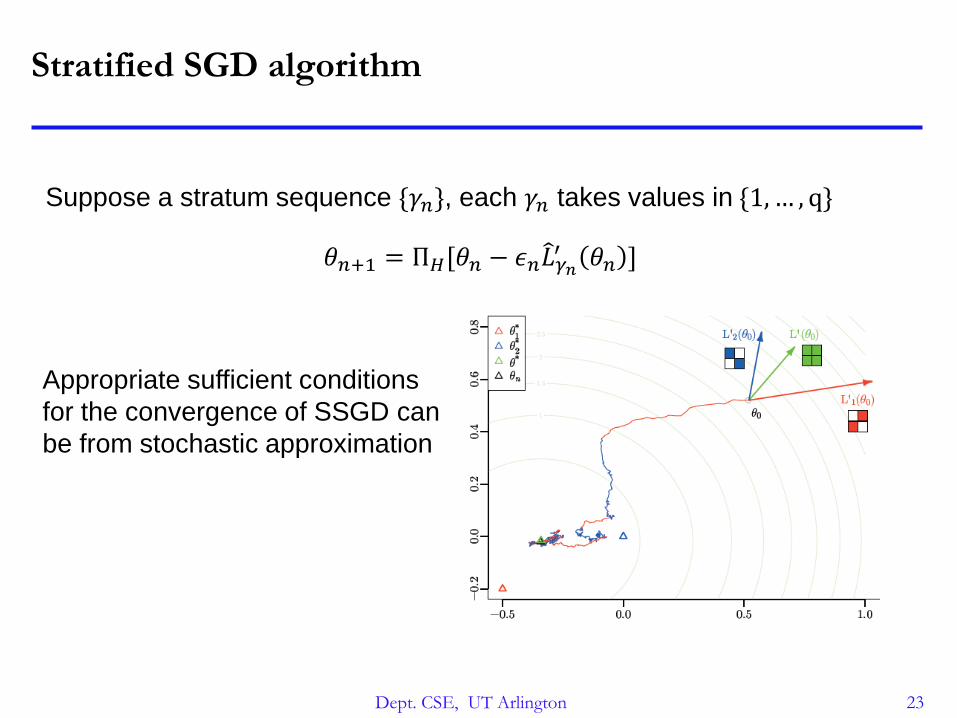
Stratified SGD algorithm
Suppose a stratum sequence {𝛾𝑛}, each 𝛾𝑛 takes values in {1, … , q}
𝜃𝑛+1 = Π𝐻[𝜃𝑛 − 𝜖𝑛 𝐿𝛾𝑛′ 𝜃𝑛 ]
Appropriate sufficient conditions
for the convergence of SSGD can
be from stochastic approximation
Dept. CSE, UT Arlington 24
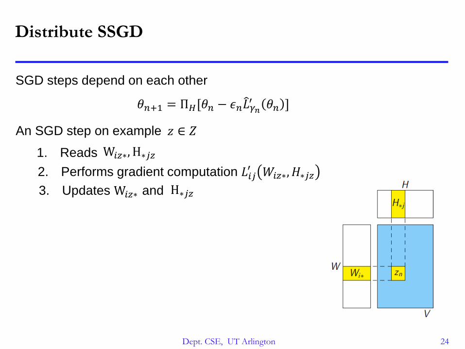
Distribute SSGD
SGD steps depend on each other
An SGD step on example 𝑧 ∈ 𝑍
1. Reads
2. Performs gradient computation 𝐿𝑖𝑗′ 𝑊𝑖𝑧∗, 𝐻∗𝑗𝑧
3. Updates and
W𝑖𝑧∗, H∗𝑗𝑧
W𝑖𝑧∗ H∗𝑗𝑧
𝜃𝑛+1 = Π𝐻[𝜃𝑛 − 𝜖𝑛 𝐿𝛾𝑛′ 𝜃𝑛 ]
Dept. CSE, UT Arlington 25
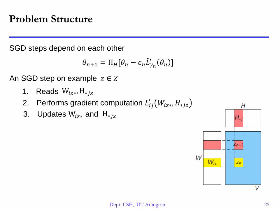
Problem Structure
SGD steps depend on each other
An SGD step on example 𝑧 ∈ 𝑍
1. Reads
2. Performs gradient computation 𝐿𝑖𝑗′ 𝑊𝑖𝑧∗, 𝐻∗𝑗𝑧
3. Updates and
W𝑖𝑧∗, H∗𝑗𝑧
W𝑖𝑧∗ H∗𝑗𝑧
𝜃𝑛+1 = Π𝐻[𝜃𝑛 − 𝜖𝑛 𝐿𝛾𝑛′ 𝜃𝑛 ]
Dept. CSE, UT Arlington 26
Problem Structure
SGD steps depend on each other
An SGD step on example 𝑧 ∈ 𝑍
1. Reads
2. Performs gradient computation 𝐿𝑖𝑗′ 𝑊𝑖𝑧∗, 𝐻∗𝑗𝑧
3. Updates and
W𝑖𝑧∗, H∗𝑗𝑧
W𝑖𝑧∗ H∗𝑗𝑧
𝜃𝑛+1 = Π𝐻[𝜃𝑛 − 𝜖𝑛 𝐿𝛾𝑛′ 𝜃𝑛 ]
Dept. CSE, UT Arlington 27
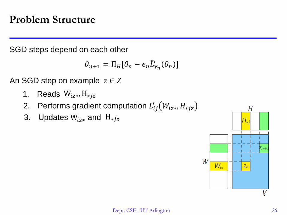
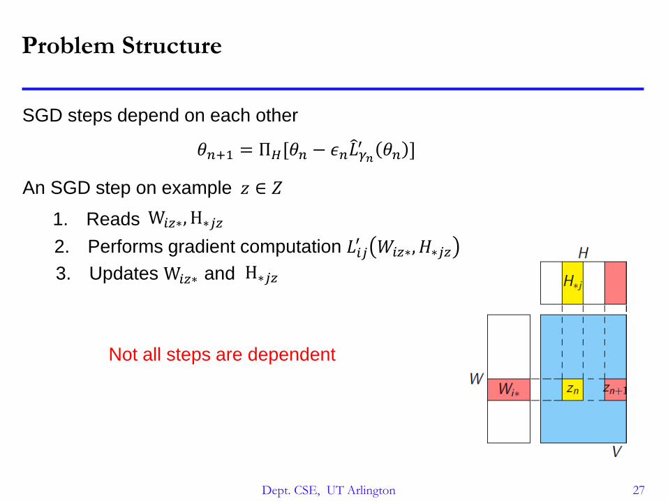
Problem Structure
SGD steps depend on each other
An SGD step on example 𝑧 ∈ 𝑍
1. Reads
2. Performs gradient computation 𝐿𝑖𝑗′ 𝑊𝑖𝑧∗, 𝐻∗𝑗𝑧
3. Updates and
W𝑖𝑧∗, H∗𝑗𝑧
W𝑖𝑧∗ H∗𝑗𝑧
Not all steps are dependent
𝜃𝑛+1 = Π𝐻[𝜃𝑛 − 𝜖𝑛 𝐿𝛾𝑛′ 𝜃𝑛 ]
Dept. CSE, UT Arlington 28
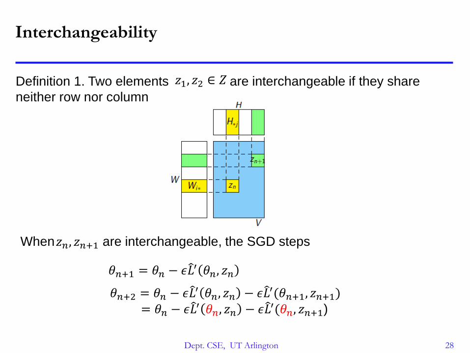
Interchangeability
Definition 1. Two elements are interchangeable if they share
neither row nor column
𝑧1, 𝑧2 ∈ 𝑍
When𝑧𝑛, 𝑧𝑛+1 are interchangeable, the SGD steps
𝜃𝑛+1 = 𝜃𝑛 − 𝜖 𝐿′ 𝜃𝑛, 𝑧𝑛
𝜃𝑛+2 = 𝜃𝑛 − 𝜖 𝐿′ 𝜃𝑛, 𝑧𝑛 − 𝜖 𝐿′(𝜃𝑛+1, 𝑧𝑛+1)= 𝜃𝑛 − 𝜖 𝐿′ 𝜃𝑛, 𝑧𝑛 − 𝜖 𝐿′(𝜃𝑛, 𝑧𝑛+1)
Dept. CSE, UT Arlington 29
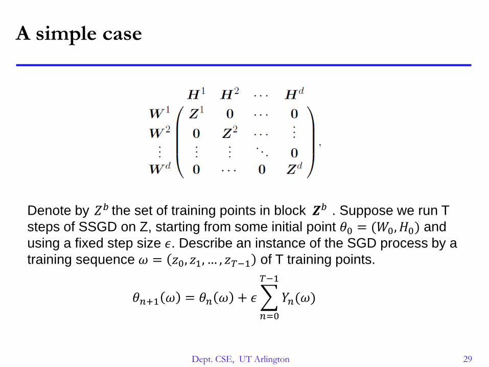
A simple case
Denote by the set of training points in block . Suppose we run T
steps of SSGD on Z, starting from some initial point 𝜃0 = (𝑊0, 𝐻0) and
using a fixed step size 𝜖. Describe an instance of the SGD process by a
training sequence 𝜔 = 𝑧0, 𝑧1, … , 𝑧𝑇−1 of T training points.
𝑍𝑏 𝒁𝑏
𝜃𝑛+1 𝜔 = 𝜃𝑛 𝜔 + 𝜖
𝑛=0
𝑇−1
𝑌𝑛(𝜔)
Dept. CSE, UT Arlington 30
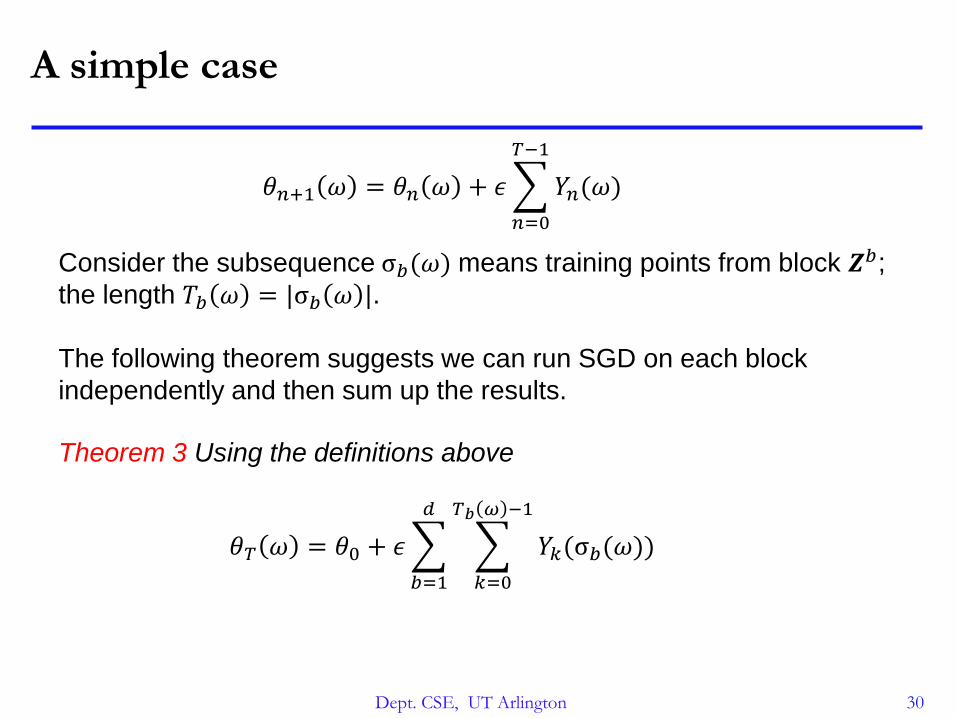
A simple case
𝜃𝑛+1 𝜔 = 𝜃𝑛 𝜔 + 𝜖
𝑛=0
𝑇−1
𝑌𝑛(𝜔)
Consider the subsequence σ𝑏(𝜔) means training points from block 𝒁𝑏;
the length 𝑇𝑏 𝜔 = |σ𝑏 𝜔 |.
The following theorem suggests we can run SGD on each block
independently and then sum up the results.
Theorem 3 Using the definitions above
𝜃𝑇 𝜔 = 𝜃0 + 𝜖
𝑏=1
𝑑
𝑘=0
𝑇𝑏 𝜔 −1
𝑌𝑘(σ𝑏(𝜔))
Dept. CSE, UT Arlington 31
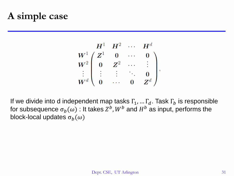
A simple case
If we divide into d independent map tasks Γ1, … Γ𝑑. Task Γ𝑏 is responsible
for subsequence σ𝑏(𝜔) : It takes 𝑍𝑏,𝑊𝑏 and 𝐻𝑏 as input, performs the
block-local updates σ𝑏(𝜔)
Dept. CSE, UT Arlington 32
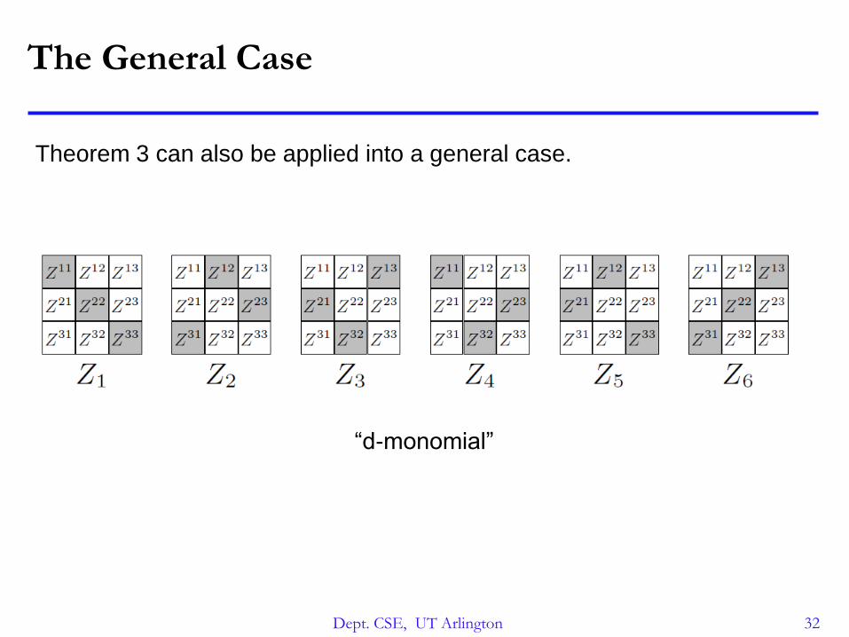
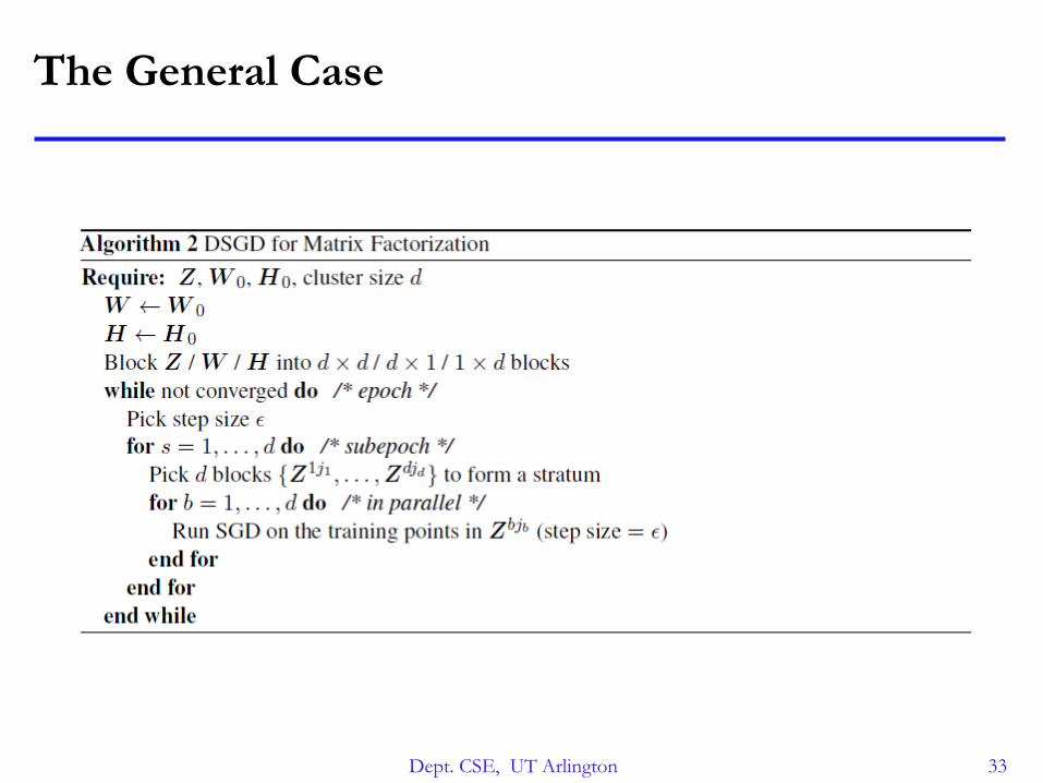
The General Case
Theorem 3 can also be applied into a general case.
“d-monomial”
Dept. CSE, UT Arlington 33
The General Case

Dept. CSE, UT Arlington 34
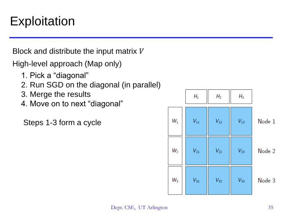
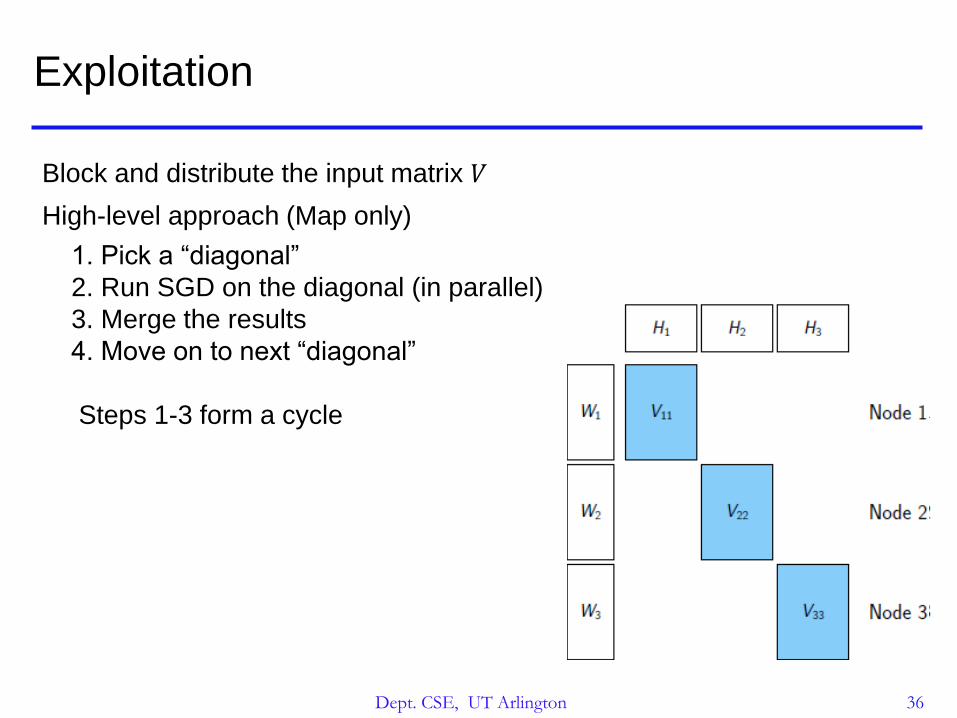
Exploitation
Block and distribute the input matrix 𝑉
High-level approach (Map only)
1. Pick a “diagonal”
2. Run SGD on the diagonal (in parallel)
3. Merge the results
4. Move on to next “diagonal”
Steps 1-3 form a cycle
Dept. CSE, UT Arlington 35
Exploitation
Block and distribute the input matrix 𝑉
High-level approach (Map only)
1. Pick a “diagonal”
2. Run SGD on the diagonal (in parallel)
3. Merge the results
4. Move on to next “diagonal”
Steps 1-3 form a cycle
Dept. CSE, UT Arlington 36
Exploitation
Block and distribute the input matrix 𝑉
High-level approach (Map only)
1. Pick a “diagonal”
2. Run SGD on the diagonal (in parallel)
3. Merge the results
4. Move on to next “diagonal”
Steps 1-3 form a cycle
Dept. CSE, UT Arlington 37
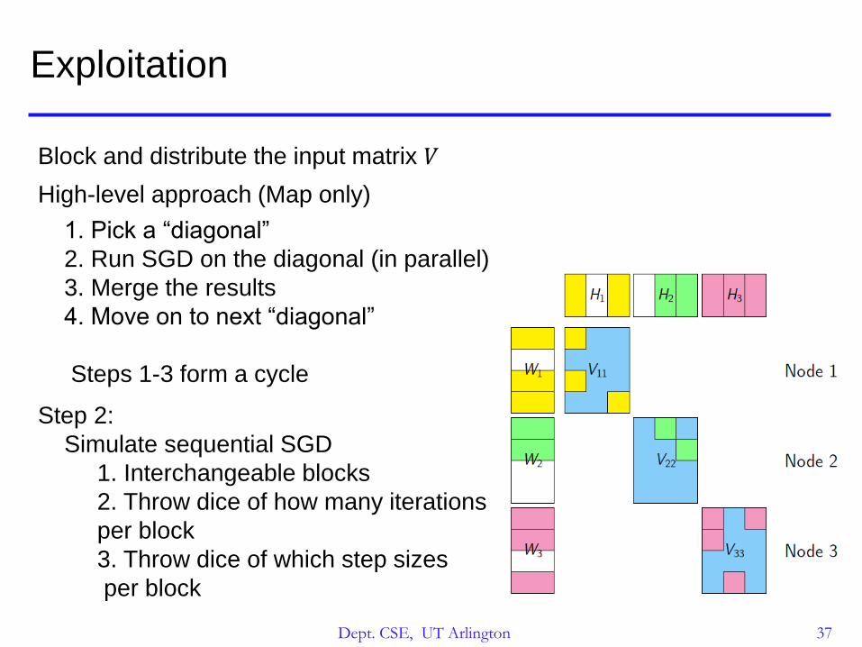
Exploitation
Block and distribute the input matrix 𝑉
High-level approach (Map only)
1. Pick a “diagonal”
2. Run SGD on the diagonal (in parallel)
3. Merge the results
4. Move on to next “diagonal”
Steps 1-3 form a cycle
Step 2:
Simulate sequential SGD
1. Interchangeable blocks
2. Throw dice of how many iterations
per block
3. Throw dice of which step sizes
per block
Dept. CSE, UT Arlington 38
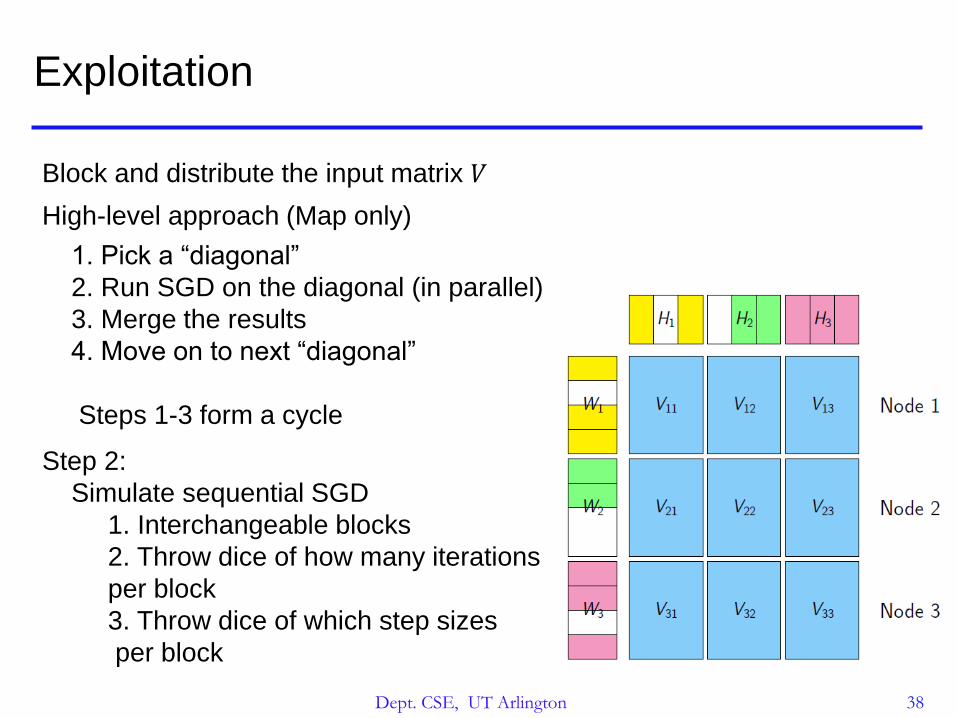
Exploitation
Block and distribute the input matrix 𝑉
High-level approach (Map only)
1. Pick a “diagonal”
2. Run SGD on the diagonal (in parallel)
3. Merge the results
4. Move on to next “diagonal”
Steps 1-3 form a cycle
Step 2:
Simulate sequential SGD
1. Interchangeable blocks
2. Throw dice of how many iterations
per block
3. Throw dice of which step sizes
per block
Dept. CSE, UT Arlington 39
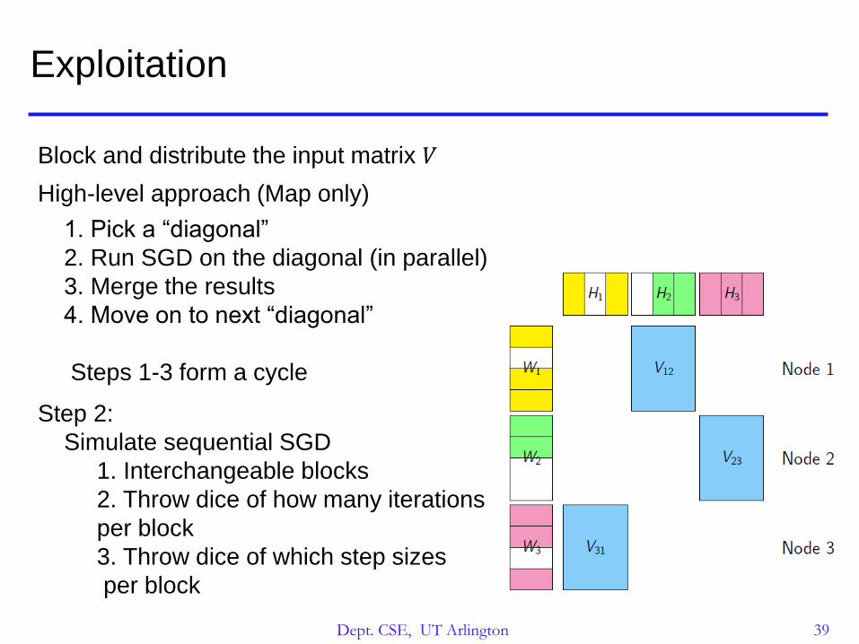
Exploitation
Block and distribute the input matrix 𝑉
High-level approach (Map only)
1. Pick a “diagonal”
2. Run SGD on the diagonal (in parallel)
3. Merge the results
4. Move on to next “diagonal”
Steps 1-3 form a cycle
Step 2:
Simulate sequential SGD
1. Interchangeable blocks
2. Throw dice of how many iterations
per block
3. Throw dice of which step sizes
per block
Dept. CSE, UT Arlington 40
Experiments
• Compare with PSGD, DGD, ALS methods
• Data
Netflix Competition
100M ratings from 480k customers on 18k movies
Synthetic dataset
10M rows, 1M columns, 1B nonzero entries
Dept. CSE, UT Arlington 41
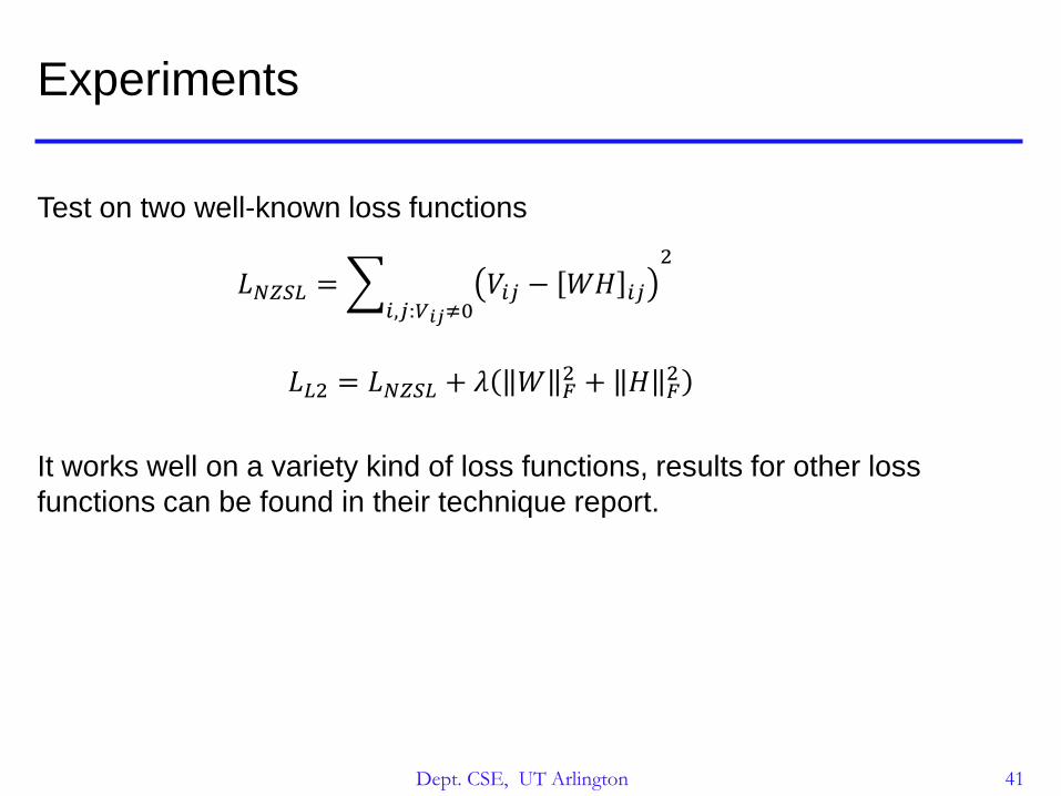
Experiments
Test on two well-known loss functions
𝐿𝑁𝑍𝑆𝐿 = 𝑖,𝑗:𝑉𝑖𝑗≠0
𝑉𝑖𝑗 − 𝑊𝐻 𝑖𝑗
2
𝐿𝐿2 = 𝐿𝑁𝑍𝑆𝐿 + 𝜆 𝑊 𝐹2 + 𝐻 𝐹
2
It works well on a variety kind of loss functions, results for other loss
functions can be found in their technique report.
Dept. CSE, UT Arlington 42
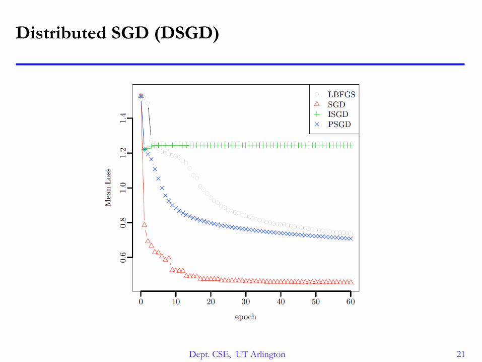
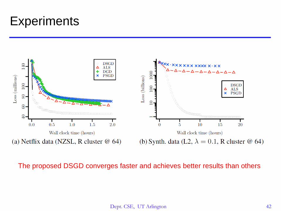
Experiments
The proposed DSGD converges faster and achieves better results than others
Dept. CSE, UT Arlington 43
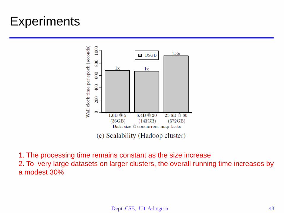
Experiments
1. The processing time remains constant as the size increase
2. To very large datasets on larger clusters, the overall running time increases by
a modest 30%
Dept. CSE, UT Arlington 44
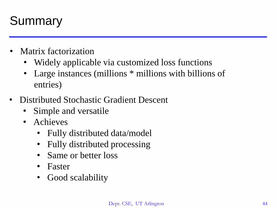
Summary
• Matrix factorization
• Widely applicable via customized loss functions
• Large instances (millions * millions with billions of
entries)
• Distributed Stochastic Gradient Descent
• Simple and versatile
• Achieves
• Fully distributed data/model
• Fully distributed processing
• Same or better loss
• Faster
• Good scalability

Dept. CSE, UT Arlington 45
Thank you!
Related Documents