Journal of Philosophy, Inc. - CMU · Journal of Philosophy, Inc. Is Ignorance Bliss? Author(s): Joseph B. Kadane, Mark Schervish and Teddy Seidenfeld Source: The Journal of Philosophy,

Journal of Philosophy, Inc.

Is Ignorance Bliss?Author(s): Joseph B. Kadane, Mark Schervish and Teddy SeidenfeldSource: The Journal of Philosophy, Vol. 105, No. 1 (Jan., 2008), pp. 5-36Published by: Journal of Philosophy, Inc.Stable URL: http://www.jstor.org/stable/20620069 .

Accessed: 08/02/2014 09:41

Your use of the JSTOR archive indicates your acceptance of the Terms & Conditions of Use, available at .http://www.jstor.org/page/info/about/policies/terms.jsp

.JSTOR is a not-for-profit service that helps scholars, researchers, and students discover, use, and build upon a wide range ofcontent in a trusted digital archive. We use information technology and tools to increase productivity and facilitate new formsof scholarship. For more information about JSTOR, please contact [email protected].

.

Journal of Philosophy, Inc. is collaborating with JSTOR to digitize, preserve and extend access to The Journalof Philosophy.

http://www.jstor.org

This content downloaded from 128.237.146.76 on Sat, 8 Feb 2014 09:41:12 AMAll use subject to JSTOR Terms and Conditions

http://www.jstor.org/action/showPublisher?publisherCode=jphil

http://www.jstor.org/stable/20620069?origin=JSTOR-pdf

http://www.jstor.org/page/info/about/policies/terms.jsp


THE JOURNAL OF PHILOSOPHY VOLUME CV, NO. 1, JANUARY 2008

4- ?I

IS IGNORANCE BLISS?*

"...where ignorance is bliss, 'tis folly to be wise."

?Thomas Gray

e are surrounded by homilies supporting the idea that human progress is intimately tied to the increase of our

knowledge. Research is justified that way, as is our enor mous investment in education at all levels, as is our support of public libraries of all sorts. Generally, we are willing, as a society, to pay a lot to make information available to ourselves and others.

It is easy to see that there may be some kinds of information that one might rationally pay not to have, if paying that price would pre vent others from learning the information as well. For example, if there were a cheap and effective means of killing all living beings, we

would have no use for that knowledge ourselves, but would pay a high price to prevent others who might want to use it from gaining the

knowledge of how to do such a thing. This paper focuses on a simpler problem, whether there is information a rational person would pay not to have for that person's private use.

The paper is organized as follows: Section i reviews the standard

Bayesian theorem about the non-negative expected worth of cost-free

sample information. Section n describes a more detailed Bayesian model that permits a more subtle understanding of what "cost-free" means in this context. Section in gives formal definitions of the value of information and cost-free information based on the formulation in section n. Section iv shows by examples that a Bayesian might pay not to receive cost-free information if the prior is improper or not countably additive. Section v reviews three extensions of the

* Research partially supported by NSF grant DMS-0139911.

0022-362X/08/0501/5-36 ? 2008 The Journal of Philosophy, Inc.

5



6 THE JOURNAL OF PHILOSOPHY

Bayesian idea to sets of probabilities, and shows that each requires or permits paying not to receive sample information. Section vi concludes with a general discussion of whether refusing to pay to be shielded from information is a criterion that should be imposed on a reasonable decision theory, and, if so, what its consequences would be.

Finally, the Appendix discusses the sense of Bayesian updating used in this paper.

There is an appealing intuitive argument supporting the idea that one should not pay not to receive cost-free information. Informally stated, it goes as follows. Suppose that one faces a decision at time t0, to be made under uncertainty. In the absence of an offer to acquire new information, one is prepared to make decision d at t0 with ex

pected utility ud. One might imagine acquiring new cost-free infor mation x at a later time t\, but then still making decision d regardless of x. From the perspective of the initial choice point at time t0, this is the same as choosing d, and has expected utility But it might be that at time t\, given x, there is a better decision than d to choose. Then from the perspective of the initial choice point, at t0, this more

complicated plan has a higher expected utility than does the choice of d. Thus, having the information x can not be harmful to one's ex

pected utility, and it might be helpful. From the perspective of the ini tial choice, at t0, the expected worth of the new information x cannot be negative.

This argument can be made rigorous as follows. Let U(d?) be your utility function, which depends on both your decision dand on 9 e @, the unknown state of the world. You have a distribution that jointly describes your probabilities for the data x e x and for 9, with joint density p(x,9). Assume that there is no cost associated with learning x.

Without the data x, you would choose d to maximize

If you were to learn the data x, you would maximize your utility with

respect to your conditional distribution p(9\x), that is, maximize

which has expectation, with respect to the unseen value of x,

I. THE EXPECTED VALUE OF SAMPLE INFORMATION

(1)

(2)

where p(x) is the probability distribution of the data x. The intuitive

argument above suggests that (3) is no smaller than (1).



IS IGNORANCE BLISS?

To show this, let d* be a maximizer of (1). [The argument works

just as well, if such a d* does not exist, for d* to be an e-maximizer of

(1).] Then for each xin (2),

= \x le U(d*,0)p(6,x)d0dx

= max \x Je U(d,6)p(6,x)d6dx, d

as claimed. This result is a familiar one in Bayesian theory, with a

II. BAYESIAN MODELS INCORPORATING PAYING NOT TO LEARN

I hold a ticket to a mystery play, and take a taxi to the theater. The taxi driver knows who-done-it and offers (threatens?) to inform me unless the tip is sufficiently large. Does it make sense to pay to avoid learning this information?

It is clear that there are circumstances in which I might pay, and that the result rehearsed in section i seems to contradict this. To un derstand the issue better, we introduce a richer decision theory that

incorporates knowledge into the utility function. In a typical decision problem, we are interested in the results at a

particular time T in the future after any decisions have been made and after enough of the state of nature has been learned to determine the impact of our decisions. In order to be flexible regarding, among other relevant matters, a "small world" versus a

"grand world" framing of a decision problem, we shall let the state of nature co describe no more than we need to make sense out of each individual decision

problem. We shall divide the collection of future outcomes into three parts.

The "state of nature" co will consist of those quantities about which a

decision maker (DM) is uncertain at some time during the decision

problem. The collection of all states of nature is d. States of nature

can include unchanging facts as well as stochastic processes. They can

(4)

Integrating both sides of (4) with respect to x, yields

xL

long history.

1 See I. J. Good, "On the Principle of Total Evidence," British Journal of the Philosophy

of Science, xvn (1967): 319-21; Howard Raiffa and Robert Schlaifer, Applied Statistical Decision Theory (Graduate School of Business Administration, Harvard University, Divi sion of Research, 1961). See also Frank Ramsey, "Weight or the Value of Knowledge," British Journal for the Philosophy of Science, xli (1990): 1-4.



8 the journal of philosophy

include amounts of wealth that might result from gambles. They can

also include inputs to decisions that might be made at later stages in a

decision problem. We assume that the state of nature stays the same

over time, but our knowledge and/or beliefs about it can change. In

particular, if the state of nature includes a random variable whose value

becomes known later, we interpret this as a change in our knowledge about the random variable rather than a change in the random variable.

The "knowledge base" is the collection of all information known by the DM. If more than one decision maker is being contemplated, each

DM has his/her own knowledge base. The knowledge base might include the knowledge that certain choices are available now or for

future decision problems as well as the various random variables that

might be available for observation and when they might become

available. The knowledge base can, and often will change over time.

We will denote the knowledge base sequence ?

{y/t : 0 < t < T],

where the subscript t denotes time. We use t = 0 to stand for "now"

when the DM starts thinking about the decision problem, and t = T

stands for the time at which all relevant information becomes available

and the DM has experienced the impact of the decision. The impact of the decision can be cumulative over a time interval, and it is possible that one might want to let T = oo to indicate that the impact never

stops accumulating. We assume that, at each time t, the DM has no

uncertainty about the corresponding value of the knowledge base y/t.

We do not, however, require that the knowledge base be nondecreas

ing over time. That is, the theory allows that a DM might forget

something that was known earlier. We will use *F with various sub- and

superscripts to denote sets of possible values for y/t at various times.

The set of acts, gambles, choices, or decisions could easily depend on

what information y/t the DM has at each time t. For example, one

cannot choose a decision that explicitly depends on a random variable

that one will not have observed at the time that the decision must

be implemented. So, we denote the set of decisions available at time t

when the knowledge base is y/t as <d(yO- An a normal-form sequential decision problem, ?>(yo) consists of sequences of choices for each

stage in the problem where each choice can be a function of what will

be known at that stage. At time t, ?(y^) for s > t might be random

because it could depend on things that might be learned between

times t and s. In an extensive form decision problem, we treat each

stage as a separate decision problem with the same T and the same

utility function but with a changing information base sequence.

Example 1. Suppose that all I care to think about now is where I will be one hour from now. Also, I care only to distinguish three possible descriptions of where I will be, namely at work, at home, or elsewhere.

We could let fl consist of the three places I could be, and we could let

<D(ô) consist of three choices, namely to stay at work, go home, or go



is ignorance bliss? 9

somewhere else. In this case, we assume that my decision will determine the state of nature with probability 1. At the time that the choice of decision must be made, I cannot have a probability dis tribution over states because the state is a function of my decision.

However, suppose that I do not have to decide which action to take for 1/2 hour. Then, I could have a marginal probability over fl for 1/2 hour until it becomes time to decide. During that 1/2 hour, I might learn things that help to influence which choice I make.

At each time t, let xFi be the set of all possible knowledge bases. Then the utility at time tis a bounded function U defined on

? x U KvJ x ?(w)].

That is, the utility at time t is a bounded function of the state, the

knowledge base, and the decision, denoted U(co,yft,d). As the knowl

edge base is allowed to (but not required to) accumulate the DM's

experiences over time, the utility at time t can depend on what has

happened in the past. Since the knowledge base is allowed to include

anticipated experiences in the future, the utility at time t can depend on what the DM anticipates might happen in the future. If <D(i//t) is

empty, that is, there are no decisions to be made, we shall fill the third

argument with the symbol .

Example 2. (Simple Decision Problem) Consider a statistical decision problem with action space n, parameter space ?, and loss function L, where L(6,a) stands for the loss that results from choosing action a when 6 is the parameter. Assume that the loss function does not change with time. Assume that no relevant data will be observed

by time T, so that the knowledge base is y/t =

y/0 for 0 < t < T. Let

<D(y/0) be the set of randomized rules, that is probability distributions over x. Assume that x is a nice enough space so that each randomized rule (5 can be constructed as the distribution of a function of a single random quantity R independent of everything else and taking values in a set ̂ . (All Polish spaces are of this type.) In particular, a non randomized rule ?a(A)

= Ia(cl) for a e X and A^h corresponds to

fsa(r) = a for all r. Let fl=?x^, where the last coordinate will hold

the value of R Let Q be the DM's prior distribution over ?. Then, for each nonrandomized choice a, we can denote the utility at time t by U((6,r),y/,?a)

= -cL(9,a) 4- b for some c > 0 and real b. For

randomized ?, U((9,r),y/,?) =

-cL(6, f$ (r)) + b. The expectation of this, over the distribution v of R, involves the usual loss of a ran domized rule:

\U((6,r),y/,?)v(dr) =

\^[-cL(e,a)+b}?(da) =

-cL(0,?) + b.




To arrive at this point in the analysis of the problem, one does not make any use of the prior distribution over ?. Hence, this much of the analysis is equally suitable for both Bayesians and frequentists.

Example 3. (Statistical Decision Problem) Expand Example 2 to include data X taking values in a set X. In this example, let <D(y/0) be a set of deterministic functions from X to K so that only non

randomized rules are available. Let fl=@XX In the typical statisti cal decision problem, we would have

(6) U((0,x),yt,S) =

-cL(0,S(x)) + b,

for all x and all t, so that utility depends on the data X = x only through the value of ?(x) and does not change with time. Up to this

point, the analysis does not depend on any probability distributions over ?. Assume now that the DM has a subjective distribution Qover ? and a regular conditional distribution P(-\9) over X given 9 for each 9 g ?. Let Q('\x) represent the posterior distribution over ?

given X = x. From (6) it follows that a Bayesian will, for each xe/, choose ?(x) equal to that a that minimizes \x L(9,a)Q(d?\x), the usual posterior risk. A non-Bayesian will compute

(7) \xU((0,x),yrt,S)P(dx\0) = -cR(6,S) + b,

where R is the classical risk function. For a maximin solution, one

would compute for each ? the infimum of (7) over 9 and then choose that ? with the largest infimum.

Example 4. (Sequential Decision Problem in Normal Form) Consider a normal form sequential decision problem in which the decision maker gets to decide how much data to observe. Suppose that the nth observation costs cn > 0 and that the terminal loss is

L(9,a), where a is the terminal action and 9 e ? is an unknown

parameter. To allow for a terminal decision before any data are ob

served, let c0 = 0. Let Xbe the potential data sequence taking values in a sequence space X. Let <D(\//o) consist of decision rules ? ? (N,d).

Here Nis either a positive-integer-valued function of data sequences xg/ such that {N = n} is measurable with respect to the first n

coordinates of xor N= 0 with probability 1 (meaning that no data will be observed). Also, d = {do, d\, d^,...) is a sequence of functions such that each dn for n ̂ 1 is a function of the first n coordinates of x and takes values in N and do is some element of X. The interpretation of such a rule is the following. If the DM decides to observe no data,

do will be the terminal action. Otherwise the DM observes N(X) > 0 observations and takes terminal action dN(X)(X). Now, ft=@XX. To




express the usual sequential decision problem in the present frame

work, we assume that

for some real b and c > 0. Once again, we have assumed that utility depends on the value of X = x only through ?(x).

Example 5. (Sequential Decision Problem in Extensive Form) Consider the same general situation as in Example 4, but this time, assume that the DM gets to reconsider her choice after each coor

dinate of X is observed. That is, the sample size N need not be a

predetermined measurable function of Xsuch that {N = n] is a func tion of the first n coordinates of X It is more convenient to express an

extended form problem as a sequence of one-stage decision problems in which the utility at each stage still depends on the utilities at other

stages. To be precise, let t0 be now and let ?x < ^ < ... be a sequence of times at which additional data might be collected depending on

what decisions are made at earlier times. Of course t0 < t\. At each time tj (i

= 0,1,...) at which a terminal decision has not yet been

made, the DM has the option of choosing to observe more data Xz+1 at time i + 1 or of making a terminal decision at the present time. If we let N denote the number of observations that will eventually be

chosen, then Nis random until a terminal decision is made. Similarly, we will let A denote the terminal action eventually chosen so that A is random until that time when a terminal action is finally chosen. For the decision problem at each time tif the set of possible decisions available is either empty (if a terminal decision was made in an earlier decision

problem) or it consists of the terminal actions k plus the decision to continue sampling. Using the notation of Example 4, the utility for the decision problem at each time t{ prior to a terminal decision is

In the framework of Examples 4 and 5, the pre-data value of a

particular decision rule is the same whether the decision problem is

put into normal form or into extensive form. In the normal form there is only one decision point among rules and each rule involves

potentially many contingent directions for what to do based on the outcomes of subsequent observations. In extensive form, there are

many decision points, each one corresponding to a change in avail

N(x) U((6,x),?t,?)

= -c L(0,dN(x)(x))- \ cn +b,




able information. Bayesian analysis yields the same assessment for a decision rule regardless in which form the decision is cast. However, for the decision theories discussed in section v, where uncertainty is represented by sets of probability distributions, the two forms are not

equivalent.2

III. THE COST AND VALUE OF INFORMATION

Section i discusses the value of cost-free information without formally defining cost-free information. To assess the cost of observing some

information or the value of the information, one needs to be able to imagine the possibility of observing (and possibly using) the infor

mation as well as the possibility of not observing it. Hence, we set up decision problems in which there is at least one stage at which the DM can choose whether or not to observe the information. Since the cost and/or value of information can change over time (imagine observing a relevant sample after having to make a decision), we

attach a time of observation to any definition of cost or value. Fur

thermore, the cost or value of information is relative to a specific decision problem.

The value of any information depends on what one does with it, so any definition will have to take into account how information is used. For example, in a Bayesian analysis, one tries to maximize ex

pected utility, while others might try to maximize the infimum of the

utility function. We will assume that the DM wants to maximize some

nondecreasing functional h of the utility function. Examples of h include the integral with respect to a probability over co and the

minimum over all co. Different functionals h correspond to different theories of decision making. To be precise, let He a real-valued function defined on the space of all bounded functions g : (l?>dt that satisfies h(g\) ^ h(g2) whenever gi(co)

< &(co) for all co. We assume

that the DM with knowledge base sequence \j/ chooses a decision rule ? in order to maximize h(U (',y/t,?)) for some time t. There are

principles of decision making that do not fit this description, but

many popular ones do. To distinguish cost from value, we think of the net value of infor

mation as some measure of the change in utility one would achieve

by observing the information and using it however one saw fit as

opposed to not observing it. We would like to define the cost to be the

2 See Teddy Seidenfeld, "When Normal and Extensive Form Decisions Differ," in

Dag Prawitz, Brian Skyrms, and Dag Westerstahl, eds., Logic, Methodology and Philosophy of Science IX (New York: Elsevier, 1994), pp. 451-63, for in-depth discussion of how normal and extensive form decision problems differ.



IS IGNORANCE BLISS? 13

change in utility one would achieve by observing the information but

then ignoring it in making decisions. This is problematic because

it may not be possible to ignore some information after observing it.

For this reason, we take a less ambitious approach and merely define

cost-free information in section m but do not quantify the cost of

information that is not cost-free.

III.I. The Net Value of Information. Suppose that a DM might be able to observe some information X at a time t\ ̂ 0 and is faced with a

decision problem as described earlier. The DM wants to say how

valuable is the information X at time t\ in the decision problem. To

do this, we embed two versions of the original decision problem in a

2-stage problem in normal form (called the extended decision prob lem) in which the first stage involves a decision at time 0 of whether or

not to observe Xat time t\. To be clear, we imagine the DM deciding at time 0 whether or not to observe X, but the actual observation of X

may occur later at time t\. The second stage of the problem will be one of the two versions of the original decision problem, one in which Xis observed (version 1) and one in which Xis not observed (version 0). The versions of the original decision problem may themselves be

sequential, but this will be immaterial for the current discussion. The set of decision rules available in the extended decision problem at

time t = 0 is <D(y/0) =

(N, do, d\) where N = 0 means to not observe X, N = 1 means to observe X, and d{ is a decision rule for version i(i

=

0,1). This matches the notation used in Example 4. To make it easier to discuss the two versions together, let y/

= {ydio be a knowledge

base for which it is known that Xis not to be observed at time ti, and let y/*

= {y/f}]=o denote the alternative knowledge base in which

it is known that Xwill be or has been observed at time t\. We assume

that yffi is the same as y/o aside from the knowledge that Xwill be

observed, so that the two versions start with essentially the same

information before the decision is made whether or not to observe X. We assume that the DM is able to determine what she would

do if Xwere observed and what she would do if Xwere not observed.

Formally, we assume that both version 0 and version 1 of the original decision problem can be solved by the DM. This could be possible even in cases in which the DM already knows that she will observe X

but still knows what she would have done if X were not to be

observed. The net value of the information Xis then defined to be

the difference

h(U(;?fA))-h(U(;?t1?0)),

where <5,- is the decision rule that the DM would use if forced to solve version i of the original decision problem for i = 0, 1 at time t.




Example 6. (Maximin Decision Maker) Suppose that the DM chooses decision rules using a maximin criterion. To be more spe

cific, consider a traditional decision problem such as the ones de scribed in Example 3 where Uis given by (6). Suppose that a decision

must be made at time t > t\. A maximin decision maker, in such a

problem, uses the functional

(8) h(g)= mfLg(0,x)P(dx\6).

Substituting the utility from (6) into (8) we obtain

h(U(;y/f,?))= inf \x[-cL(0,0(x)) + b]P(dx\0),

for each rule ?^(D(y/f). In version 0, all decision rules ? have to be constant as a function of x. Hence, we have

h(U(;y/t,?))= inf[-cL(0,0) + b], 9 e 0

for each Se(D(y/t). So, the net value of X would be

sup inf(-cR(0,0) + b)- sup inf (-cL(0,0) + b).

where R(9,?) is the classical risk function

R(0,?) =\xL(6,?(x))P(dx\6).

As a specific example, consider the following augmentation of the example presented by Leonard Savage3 in which we give a specific data distribution. Let fl=@XX where the parameter space ?

= {1,2} and the sample space X=l, 2,3. Let the space of terminal decisions N = {1,2}. At time to the DM must decide whether to observe X taking values in X. At time t\ > t0, the DM has to choose one of the two

terminal actions from K. Let X have the following conditional dis tribution given 0:

0.5 if i = j = 1 or i = j

= 2 or i = 3, Pr(X= i\6 = j) = I0'5 if i=j= lc

J \ 0 otherwise

The random variable Xidentifies 9 with probability 0.5 (when X^ 3) and it is irrelevant with probability 0.5 (when X =

3). Let the utility

3 Savage, The Foundations of Statistics (New York: Wiley, 1954), p. 170.




have the form of (6) with c= 1, b = 0 and consider the following loss function regardless of whether X is observed:

for all t, 9, and x. Intuition suggests that Xhas value for the DM unless 9 is known with certainty. If Xis not observed, then the maximin decision is to choose terminal action a = 1. In this case h(U (-,^,1))

= ?1. If Xis to be observed, the maximin rule is any Bayes rule with respect to the least favorable prior. The least favorable prior is Pr(0=l)

= l, and the collection of Bayes rules is the set of rules ?a where, for each a, ?a (1)

= <5a (3)

= 1 and ?a (2) randomizes between 1 and 2 with Pr((5a (2)

= 1)

= a for arbitrary a e [0,1]. The risk functions of these rules are

For all of these rules, h( U (',y/t,?a)) = ?

1, so the maximin decision maker

assigns 0 net value to the information X, contrary to intuition.

Savage claims that maximin decision making is "utterly untenable for statistics" based on the fact that the seemingly relevant data in

Example 6 has 0 value (ibid., p. 170). (We will see in section in.2 that the Xin that example is cost-free.) Savage contrasts the maximin rule

with maximin-regret, which we describe next. Example 7. (Maximin-Regret Decision Maker) A variation on

maximin decision making is to shift the utility function so that the maximum value is the same in every state, typically 0. In symbols, replace Uby

(9) U'(co,y/t,?) =

U(co,y/t,d) -

max U(o),y/t,3). ?

The maximin-regret decision maker then behaves the same as a maximin decision maker whose utility is U' instead of U. In particular, for the calculations that appear in Examples 3 and 6, we replace L(9,m) by L(9,-)

? mina L(9,a) everywhere and set b = 0 wherever it occurs.

The functional h is still (8). Now, reconsider the example of Savage (ibid., p. 170) from this

point of view. The modified loss function is

That is,

U((6,x),y/t,?) =

-L(6,?(x)),

(9 if 0=1, a = 2, L\e,a)

= { 2 if 6 = 2, a = 1,

0 otherwise.




If the DM does not observe X, the maximin-regret decision is the

randomized rule 5 that chooses a = 1 with probability 9/11 and chooses a = 2 with probability 2/11. For this rule, h(U(-,y/t0,?)

= ?

18/11. However, if Xis observed, the risk function of the general randomized rule S? that chooses a ? 1 with probability when X ? i is observed equals

The maximin rule corresponds to ?i = 1, ?2

? 0, and ?3

= 9/11 which

has h(U ('yi/St??)) ?

?9/11. So, the maximin-regret decision maker

assigns net value (?9/11) ?

( ?

18/11) =9/11 to the information X

Savage suggests that maximin-regret decision making is not as

prone to the objection of assigning zero value to relevant data (ibid.,

p. 200). However, Giovanni Parmigiani4 shows that there are exam

ples in which maximin decision making gives positive net value to

data that are assigned zero net value by maximin-regret. Example 8. (Bayesian Decision Maker) Suppose that the DM

wants to choose the decision rule 5 at time t that maximizes ex

pected utility. Let the DM's distribution (now) for co be P. Then

Next, consider the special case of Example 3 in which co ? (6, x). Then the net value of the information Xis the difference between the

extreme terms in (5) if the following two conditions hold:

the utility has the simple form U((6, x),y/t,?) = U(?(x),?) for all t, and

(X, 6) has a joint density p(x, 6) with respect to Lebesgue measure.

In Savage's example, suppose that the Bayesian DM starts with

Pr(? =

1) =

p. Without observing X, it is easy to see that a Bayesian DM will choose a=lifp> 2/11 and will choose a = 2 if p < 2/11. Either action can be chosen if p

= 2/11. Call this Bayes decision

?fi. Then

If X is observed, then the Bayesian DM chooses a = 1 if X = 1 and

chooses a = 2 if X = 2. If X = 3, the DM uses the same Sp she would

h(U(;ffftf?))=\[lU((Ot}fftf?)P(d(o).

(10)

4Parmigiani, "Minimax, Information, and Ultrapessimism," Theory and Decision, xxxiii (1992): 241-52.




have used if Xhad not been observed. For this rule h(U(',y/t,?fi)) equals one-half of (10) (corresponding to X =

3) plus 0.5 - p (cor

responding to X^ 3). The net value of Xfor the DM who believes

Pr(0 =

1) =

p a priori is

Notice that the largest possible net value occurs at p = 2/11 and

equals 9/11, the same net value assigned by the maximin DM. The least favorable distribution in the maximin-regret problem is

Pr(0 =

1) = 2/11 for both version 0 and version 1.

Example 9 (F-Maximin Decision Maker) We will discuss T maximin decision rules in more detail in section v. For now, we can

understand T-maximin decision making as a variant on Bayesian decision making in the following sense. One replaces the single distribution P over states used by the Bayesian decision maker in

Example 8 by a closed convex set <P of distributions. Then, one ranks decision rules by

In Savage's example, suppose that the T-maximin DM chooses

^[piife]- If Pi - 2/11 <

p2, then the DM behaves just like the

maximin-regret DM because the infs in (12) will occur at the least favorable distribution in both version 0 and version 1. If p2 < 2/11, the DM will behave like the Bayesian in Example 8 with p

= p%. If pi >

2/11, the DM will behave like the Bayesian with p ?

p\. The net value of Xcan be found for these last two cases in (11).

III.2. Cost-Free Information. This section formally defines what we mean by saying that observing information X at a specific time t\ is cost-free. We will do this in a manner that does not depend on the decision principles to which one adheres. In order for information at a specific time to be cost free for every mode of decision making, we require several conditions. First, we require that it is possible not to observe Xat time t\. Second, we require that the information be

decision-theoretically ignorable, meaning that every decision rule that is available without the information is also available with the informa tion so that one could ignore the information when choosing a de cision rule. To make this more precise, let yr

= {yst}T=o be a knowledge

base sequence for which it is known that X is not to be observed at time t\9 and let ̂*

= {yff}J= 0 denote the alternative knowledge base

sequence in which it is known that Xwill be or has been observed at time t\. To say that observing X at time t\ is decision-theoretically

(11)

(12)




ignorable, we mean that for each decision time t and each 0?<D(y/t) there is a b*e<D(\f/f) which does exactly what b would do under all states of nature that are still possible, essentially ignoring X to the extent possible. To put it another way, learning Xat time t\ does not eliminate any decision rules from consideration. There is a subtle issue that should be addressed at this point. Suppose that, even if the

DM does not observe Xat time t\, she will nevertheless observe it at some later time. A simple example will illustrate the issue.

Example 10. Let N consist of two points N = {?o,ai}. Let X be a Bernoulli random variable that we believe to be independent of

everything that is relevant in this decision problem. Let t\ = 0, and let 0 < t2. Suppose that X will be observed by time t2 under all

circumstances, but we have the option of observing it at time t\.

Suppose also that, at time t2, we must choose between two decision rules ?0= oq and di(X)

= ax- That is, we can either pick action clq by choosing b0 or we can choose b\ which randomizes between oq and a\

by using X: if X = 0 then we will pick a0 and if X = 1 we will pick ax. So, the terminal action is not finally decided until time ^ when X will

definitely be known. If we choose to observe Xat time t\ and X = 0 is

observed, then the only terminal action that will be available to us is a$

regardless of whether we choose decision rule b0 or S\. Nevertheless, the decision rule b\ is still available at time t2. It just happens that

we already know that S\(X) = a0.

In Example 10, X is decision-theoretically ignorable because the decision rule bi is still available when it comes time to choose regard less of the fact that we might already know that it will make the same choice as b0. When it comes time to make our decision, we are in the same situation regardless of whether we observed X = 0 at time t\ or at some later time.

Information Xthat is decision-theoretically ignorable will be called

cost-free if, for every state of nature co, every knowledge base sequence y/, every time t, and every de(D(y/t),

(13) U(co,\irt,?) =

U(cD,yf*?*),

where (5* was defined above as the decision rule in <D(\jff) that makes the same choices as b under all circumstance. In other words, if the DM ignores X, she will achieve the same utility as if X had not been observed. In particular, there can be no fee for merely observing X.

Example 11. (Return to Example of Savage) This example is set

up in the second half of Example 6. In the notation of this section, let

<D(yfti) contain all randomized decision rules that are just probabil ities over x = {1,2}, and let <D(y/%) consist of all randomized decision rules that are functions of X. It is easy to see that for each rule bp in




<D(y/t ) that chooses a = 1 with probability p and chooses a ? 2 with

probability 1 ? p, there is a ?p* e <D(\ff%) such that ̂(x) =

<5^ for each x = 1, 2, 3. Hence, Xis decision-theoretically ignorable. It is also easy to see that U(co,yft,?p)

= U(co,\iff,df) for all p, y/, and t. Hence, the

information Xis cost-free in this example. Now return to the example at the start of section n.

Example 12. (The Taxi Driver) Recall that I hold a ticket to a

mystery play and take a taxi to the theater. The taxi driver knows who done-it and offers to inform me unless the tip is sufficiently large. Does it make sense to pay to avoid learning this information? Assume

that I am committed to attending the mystery so that I need not con

sider the possibility of doing something else. This makes the infor mation offered by the taxi driver decision-theoretically ignorable because I have no decision points after I choose the tip. For this rea

son, we will write the utility as U(co,y/t,D) to indicate that no decisions are available in either version 0 or version 1 of the problem. If we

determine that the information is not cost-free, then we are faced

with the extended decision problem of whether to pay not to observe it. For simplicity, suppose that I am contemplating, at time 0, only two

different tips, 0 and v > 0, where v is sufficiently large to prevent the

taxi driver from telling me who-done-it. At present, I believe that

attending the mystery will have a random (that is, unknown) effect on

several of my emotions at certain times in the future with various

probabilities that reflect my opinion of how well the mystery is

produced and what I know at the time of the play. In particular, the

play offers the possibility of suspense and surprise. If I do not know

who-done-it, the probabilities of high levels of suspense and surprise are larger than if I do know. Similarly, if I do not know who-done-it, the probability of boredom is smaller than if I do know. A poorly

written/produced play might cause boredom even if I do not know who-done-it. We can interpret the information about who-done-it to

be data that might be added to my knowledge base at or before time

T, when the mystery will be finished. The taxi driver has offered me

the choice of which tip to give, which is assumed to be equivalent to

whether or not to obtain the information of who-done-it. No further

decision point is available after this decision is made. To be explicit, let ft =

{1,..., } X % where i is the number of

characters in the play, and T is a space each of whose elements

specifies a set of values for the various aspects of the quality of the

play. Suppose that I have a distribution \i over the space T that gives my opinion of the play. Let Yo be my current knowledge base, and assume that I will not learn anything else before I have to choose a tip at time t\, so that y/ti

= y/0. For each i= 1,.. > t\, and x > 0 let yft,i,x




be the augmented knowledge base at time t assuming that I learned that character i done-it before attending and assuming that I have

paid x as a tip. Let y/tfX be the corresponding knowledge base if I do not learn who-done-it but pay a tip of x. To avoid certain philo sophical difficulties, suppose that, prior to getting in the taxi I have

already considered the possibility that I might learn who-done-it before seeing the play and that I had already considered the pos sibilities of giving various tips even if I had never dreamed that the two might be related. Assume, for simplicity, that neither U((i,y), y/tfX,n) nor U((i,y) ,y/t^x,\3) depends on i for fixed y e <Y and fixed x. These assumptions merely mean that I have no particular in terest in which character did it. Fix t > t\ and x > 0 and let

Ux=\rU((i,y),\irt,i,x&)p(dy) and Ux=\r U((i,y), y/tyX,D) [i(dy). These are respectively the expected utilities that I would have calculated at time t after giving a tip of x under the assumptions of learning and not learning who-done-it before seeing the play.

It makes sense that Ux < Ux for all x, that is, it is better not to know

who-done-it, regardless of what tip I might give. Also, Ux > Uw, and jjx > jjw wnenever x< w, meaning that my utility goes down with the size of the tip, both in the case of learning and of not learning who done-it. The expected utility of choosing tip v is then Uv while the

expected utility of choosing tip 0 is U0. The fact that Uv < Uv makes the information not cost-free. Which tip we should give hinges on

whether or not Uv > Uq, the only comparison not fixed so far by the

problem description. This comparison is between the disutility of the large tip v, on the one hand, to the disutility of ruining the

experience of the play on the other.

Examples 4, 5, and 12 are cases in which the data are not cost-free.

IV. THE VALUE OF COST-FREE INFORMATION

Assume that Xis cost-free. Then a DM who maximizes expected utility will not want to pay to avoid learning X. To see this, argue as follows. Let P(dx,dco) stand for the joint distribution of Xand co. Even though we have assumed that Xis a function of co, this joint distribution still makes sense as a measure. Also, let P(dco I x) stand for the posterior distribution of co given X = x. Let <S* be the decision that the DM

would make without observing X, and let S*' be the corresponding rule that observes X but ignores it. Then for each t

(14) \x\aU((o,?t^)P{dx,d(D)

is the DM's expected utility at time t without observing X If X = x were observed, the DM would choose the decision 8 to maximize

(15) \aU(co,y/t}X,S)P(dco\x).




For each x, we use (13) to generalize (4) as

(16) max lnU(<jQ,y/t,x,?)P(dco\x)

> \nU(cD,y/ttX,?*')P(dco\x)

=\nU(w,y/t,?*)P(dco\x).

The rest of the argument is virtually identical to that in section i.

The result above (as well as the one in section i) applies only to

joint probability distributions on the data and state of nature that are

countably additive and proper, as the following examples show. Both of these examples assume that the available data are cost-free, that is, the utility function is the same before and after observing the data.

What fails from the result above and that of section i is that finitely additive and improper joint distributions do not always factor into

marginals and conditionals the way that countably additive joint distributions do.

Example 13. (Finitely, But Not Countably Additive Distri

butions) Suppose that there are two states of the world, A and B, each of which has probability 0.5 in your current opinion. Imagine that you can observe a positive integer N. If A is true, the integer N has a geometric distribution, as follows:

P(n\A) = (l/2)n,

for each integer n > 0. However, if B is the case, the integer N is

uniformly distributed on the integers in your opinion. There are

many such finitely additive distributions,5 but they all have the prop erty that

P(n\B)=0

for each integer n > 0. If a particular integer, say N = 3, is observed, an easy application of

Bayes's Theorem shows that

P(A\N=3) = l

and in fact, this is true whatever value n of Nis observed. Hence you are in the peculiar state of belief that although your prior is even

between A and B, you know that conditional on the observation of N,

regardless the value of N, you believe with certainty that A is true.

5 See Joseph B. Kadane and Anthony O'Hagan, "Using Finitely Additive Probability:

Uniform Distributions on the Natural Numbers," Journal of the American Statistical

Association, xc (1995): 626-31; also Oliver Schirokauer and Kadane, "Finitely Additive Distributions on the Natural Numbers: Shift Invariance," Journal of Theoretical Probability, xx, 3 (2007): 429-41.




Which then is your prior, what you believe now, or what you know you would believe if you could observe iV?6

Suppose that you currently hold a ticket that pays $1 if ̂ is true, and

?$1 if A is true. Currently your expected winnings are $0. However,

you know that if you were to obtain the integer N9 your expected winnings would be ?

$1. Would you pay $0.50 not to receive the data? It seems that you would have to. Where does the proof given above fail for finitely but not countably

additive distributions? The proof fails because conditional probability does not work the same way for finitely additive and countably addi tive distributions. Technically, it concerns the failure of conglomer ability,7 that is

P(A\N=n)>P(A) for all n > 0.

Example 14. (Improper Distributions) There are Bayesians who use improper distributions (that is, those that integrate to infinity) as a way of modeling "ignorance"; sometimes these priors are called "reference" or

"objective." The simplest case of these arise as ap

parent results of limits of proper priors. Suppose for example that the

datum xis normally distributed with mean Wand precision (inverse variance) 1. Suppose also that Whas a normal prior with mean 0 and

precision r. Then it is well known that the posterior distribution of W

given x is again normal with mean the precision-weighted average of x

and 0, and precision equal to r + 1. Now imagine that r approaches 0, so the variance of the prior goes to infinity. Then the posterior of W

given x approaches a normal distribution with mean x and precision 1. This is the same answer that would have been obtained from using an improper uniform distribution on W9 and doing a formal cal culation of the posterior. The hope is that because the improper distribution is the limit of proper posteriors, nothing "bad" happens in the limit.

Now suppose that the precision R of the normal observation is not

known, but that the conjugate prior is imposed, that is, Wgiven R = r

is normal with mean 0 and precision rr, and R has a T(a, ?) distribution with a > 1. The general form of the posterior, given X = x

is then8 as follows: the posterior on W given R = r is normal as before,

6 We explored this phenomenon in Kadane, Mark Schervish, and Seidenfeld,

"Reasoning to a Foregone Conclusion," Journal of the American Statistical Association, xci

(1996): 1228-35. 7 For more on this, see Bruno de Finetti, Theory of Probability, Volume 1 (New York:

Wiley, 1974). 8 See Morris Herman DeGroot, Optimal Statistical Decisions (New York: McGraw-Hill,

1970) pp. 167ff.




with mean the precision-weighted average of x and 0 with precisions rand t respectively, and the posterior of R is T(a + 1/2, ? + tx2/ [2(t + 1)]). As t approaches zero, the conditional posterior distribu tion of Wgiven R= r is as before, normal with mean x and precision r, and the posterior of Ris T(oc + 1/2, ?).

Now, we set up a decision problem in which one would pay to avoid

learning X. Let a2 = l/R, the usual variance parameter. In the nota tion used earlier, with co = (W, R), let U(co,y/t,?)

= a2. Note that the

utility depends only on the value of a), not on any decisions. In this

case, before any data are observed,

(17) E[U(co,?o>0)] =

E(a2) =

?/(a -

1),

and after X = x is observed say at time t\9

? E{U(w,y/?,?)]

= (ci\X

= x) -1/2'

the same for all x, which is strictly smaller than (17). A similar result holds no matter how many observations one con

templates. For example, suppose that X = (X1?...,XW) is a vector of

n observations that are conditionally independent and identically distributed given (W, R) with the same distribution described above. In this case, (1) is the same as above, namely ?/(cc

- 1). With n ob

servations, the posterior distribution of R derived from the improper prior is r(a+n/2, ?+ 2n (#/

? x)2/2), where x = lZn Xj/n. Using the

i=l i=l

same utility C7(a),^5) =

a2, we see that (2) equals

1 71

j3 + -2(*,-x)2 (18)

a + --l.

To calculate (3), recall that the distribution of X is defined by first

conditioning on (W, R) and then integrating with respect to the distribution of (W, R). The integral of (18) with respect to the con ditional distribution of Xgiven (W, R)

= (w, r) is easily computed as

n

Integrating this with respect to the marginal distribution of (W, R) yields

l(n-l)j8 ? + 2 a -

1 n

a+ - - 1




which is then (3) in this example. A little algebra shows that (3) is still smaller than (1). Indeed, the difference is ? ?/[2(oc

? 1) (a

? 1 + n/2)]. One would pay, say, half of this amount to avoid seeing the data.

The issue in Example 14 is that the posterior mean of a2 differs from the prior mean by an amount that has negative prior mean. That

is, even before collecting the data, we expect the posterior mean to be smaller than the prior mean. Just as in Example 13, it is fair to ask what your prior mean of a2 really is, what you think now or the mean of what you know you would think if you were to observe X. Just as

before, you can be confronted with the prospect of paying not to see the data X, because it would change your mean of a2 in a way unfavorable to you. Hence even in the apparently simple case of a

sample of observations from a univariate normal distribution, with

conjugate priors and flattening on the mean, the same issue arises of

potentially paying not to see the data.

V. GENERALIZATIONS OF BAYESIAN DECISION THEORY INVOLVING

SETS OF PROBABILITIES

There is recent interest in decision theories involving sets of prob abilities. The intuitive idea behind them is to relax the requirement of knowing one's opinion about p(x, 9), but doing so in a way dif ferent from the "reference" -

"objective" -

"non-informative" prior school. We study three of the leading such theories here. In all of this

discussion, the joint distributions will be countably additive and all data will be cost-free.

Of the three decision rules we discuss, perhaps the most familiar one is T-Maximin.9 This rule requires that the decision maker ranks a

gamble by its lower expected value, taken with respect to a closed, convex set of probabilities, <P, and then to choose an option from whose lower expected value is maximum.10 The T-Maximin decision rule creates a preference ranking of options independent of the alternatives available in A: it is context independent in that sense. But

9 When outcomes are cast in terms of a (statistical) loss function, the rule is then

T-Minimax: rank options by their maximum expected risk and choose an option whose maximum expected risk is minimum.

10 This decision rule was given a representation in terms of a binary preference

relation over Anscombe-Aumann horse lotteries by Itzhak Gilboa and David

Schmeidler, "Maxmin Expected Utility with Non-Unique Prior," Journal ofMathematical Economics, xvm (1989): 141-53, has been discussed by, for example, James O. Berger, Statistical Decision Theory and Bayesian Analysis (New York: Springer, 1985, 2nd ed.), section 4.76. And recently by Peter D. Grunwald and A. Philip Dawid, "Game Theory,

Maximum Entropy, Minimum Discrepancy, and Robust Bayesian Decision Theory" (Technical Report 223, University College, 2002) who defend it as a form of Robust

Bayesian decision theory.




r-Maximin corresponds to a preference ranking that fails the so

called (von Neumann-Morgenstern's) "Independence" or (Savage's) "Sure-thing" postulate of SEU (Subjective Expected Utility) theory.

The second decision rule that we consider, called ivadmissibility ('?* for "expectation"), was formulated by Isaac Levi.11 E-admissibility constrains the decision maker's admissible choices to those gambles in A that are Bayes for at least one probability P e <P. That is, given a choice set A, the gamble / is inadmissible on the condition that, for at least one Pe<P, / maximizes subjective expected utility with

respect to the options in A-12 Savage13 defends a precursor to this de cision rule in connection with cooperative group decision making, inadmissibility does not support an ordering of options, real-valued or otherwise, so that it is inappropriate to characterize inadmissibility by a ranking of gambles independent of the set A of feasible options. However, the distinction between options that are and are not Er admissible does support the "Independence" postulate. For example, if neither option / nor g is inadmissible in a given decision problem

A, then the convex combination, the mixed option h = oe/(B (1 ?

a)

g(0 < a ^ 1) likewise is ̂ -inadmissible when added to A- This is

evident from the basic SEU property: the expected utility of a con vex combination of two gambles is the corresponding weighted average of their separate expected utilities; hence, for a given Pe<P the expected utility of the mixture of two gambles is bounded above

by the maximum of the two expected utilities. The assumption that neither of two gambles is inadmissible entails that their mixture has

P-expected utility less than some inadmissible option in A The third decision rule we consider is called Maximality by Peter

Walley,14 who appears to endorse it (ibid., p. 166). If a gamble f gA is such that there is no other gamble g bA strictly preferred to ? then

/ is admissible by Maximality. That is, / is a Maximal choice from

A provided that there is no other element gÂ that, for each P e <P, carries greater expected utility than /does. Maximality (under differ

nLevi, "On Indeterminate Probabilities," this journal, lxxi, 13 (July 18, 1974): 391-418; and Levi, The Enterprise of Knowledge (Cambridge: MIT, 1980).

12Levi's decision theory is lexicographic, in which the first consideration is E

admissibility, followed by other considerations, for example, what he calls a Security Index. Here, we attend solely to E-admissibility. 13

Savage, op. cit., section 7.2. Savage's analysis of the decision problem depicted by his Figure 1, p. 123, and his rejection of option b, p. 124 is the key point. 14

Walley, Statistical Reasoning with Imprecise Probabilities (New York: Chapman and

Hall, 1990). There is, for our discussion here, a minor difference with Walley's for mulation of maximality involving null-events. Walley's notion of maximality requires, also, that an admissible gamble be classically admissible, that is, not weakly dominated with respect to state-payoffs.




Utility axis

co-, 0.25 0.75 co2

P(cd2) axis

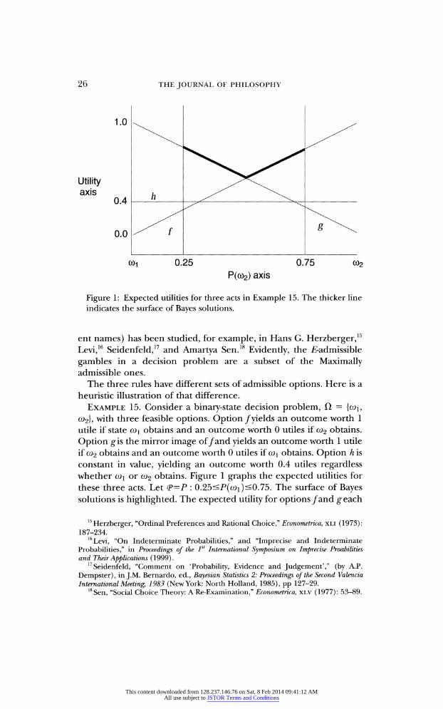
Figure 1: Expected utilities for three acts in Example 15. The thicker line

indicates the surface of Bayes solutions.

ent names) has been studied, for example, in Hans G. Herzberger,15 Levi,16 Seidenfeld,17 and Amartya Sen.18 Evidently, the ̂ -admissible

gambles in a decision problem are a subset of the Maximally admissible ones.

The three rules have different sets of admissible options. Here is a

heuristic illustration of that difference. Example 15. Consider a binary-state decision problem, fl =

{co1? C6>2}, with three feasible options. Option /yields an outcome worth 1 utile if state W\ obtains and an outcome worth 0 utiles if co2 obtains.

Option gis the mirror image of /and yields an outcome worth 1 utile if a>2 obtains and an outcome worth 0 utiles if co\ obtains. Option h is constant in value, yielding an outcome worth 0.4 utiles regardless whether a>i or 0)2 obtains. Figure 1 graphs the expected utilities for these three acts. Let (p=P : 0.25<P(coi)<0.75. The surface of Bayes solutions is highlighted. The expected utility for options/and g*each

15 Herzberger, "Ordinal Preferences and Rational Choice," Econometrica, xli (1973):

187-234.

16Levi, "On Indeterminate Probabilities," and "Imprecise and Indeterminate

Probabilities," in Proceedings of the 1st International Symposium on Imprecise Proabilities and Their Applications (1999).

17Seidenfeld, "Comment on 'Probability, Evidence and Judgement'," (by A.P.

Dempster), in J.M. Bernardo, ed., Bayesian Statistics 2: Proceedings of the Second Valencia

International Meeting, 1983 (New York: North Holland, 1985), pp 127-29. 18 Sen, "Social Choice Theory: A Re-Examination," Econometrica, xlv (1977): 53-89.




has the interval of values [0.25, 0.75], whereas h of course has constant expected utility of 0.4. From the choice set of these three

options A={f, g, h} the T-Maximin decision rule determines that his

(uniquely) best, assigning it a value of 0.4, whereas /and geach has a

T-Maximin value of 0.25. By contrast, under E-admissibility, only the

option h is E-inadmissible from the trio. Either of /or gis E-admissible.

And, as no option is strictly preferred to any other by expectations with respect to <P, all three gambles are admissible under Maximality.

We link this observation to the debate about the value of new

information by considering a sequential decision problem in which the decision maker has the opportunity to postpone a terminal de cision in order to learn the outcome of a mixing variable, a vari able used to convexify the option space. Let the mixing variable a

equal 1 or 0 as a fair coin lands Heads up or Tails up on a toss, so that

P(ot =

1) =

P(a =

0) = .5. Assume, also, that a is independent of the

states, ft, over which the pure options are defined, so that each P e <P,

P(a, co) -

.5P(co). As a modification of Example 15, consider the mixed options m,

and n, defined as follows

m = ocf ? (1 -

a)g

n = ag 0 (1 -

a)/.

Thus, m is the mixed act that uses the fair coin to bet on co\ if Heads

(H) and to bet on co2 if Tails (T). Likewise, n is the dual mixed act that uses the same fair coin to bet on co2 if Heads and to bet on coi if Tails. Note that m and n each carry a constant expected utility, .50. That is, these are options of determinate risk, despite the fact that uncertainty is with respect to the convex set of probabilities <P. Last, let the option Status quo denote no change in expected utility, with constant value 0.

The next two examples, sequential decision problems 1 and 2, are cast in extensive form. The three decision rules we discuss with these

examples, each a generalization of Bayesian decision making when

uncertainty is represented by a set of probability distributions rather than a single probability distribution, yields different results when extensive form decisions are changed to their normal form. Thus, in what follows we have a different situation than we saw in Examples 4 and 5. In those examples uncertainty is represented by a single probability distribution. Then, each of these three rules yields the same Bayesian analysis either in extensive form or in normal form.19

19 See Seidenfeld, "When Normal and Extensive Form Decisions Differ" (op. cit.).




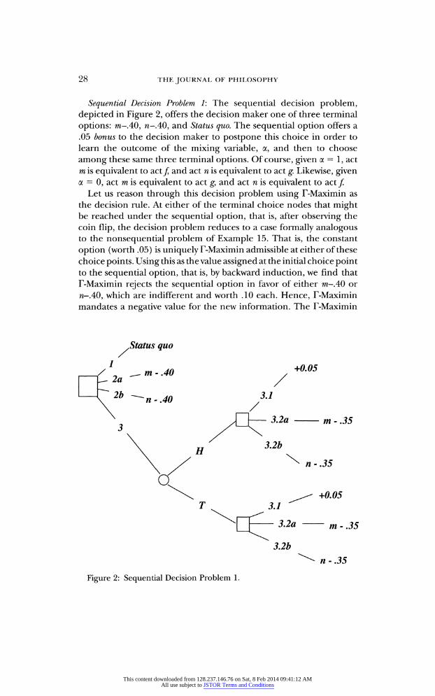
Sequential Decision Problem 1: The sequential decision problem, depicted in Figure 2, offers the decision maker one of three terminal

options: m-AO, n-AO, and Status quo. The sequential option offers a .05 bonus to the decision maker to postpone this choice in order to learn the outcome of the mixing variable, a, and then to choose

among these same three terminal options. Of course, given a = 1, act m is equivalent to act / and act n is equivalent to act g. Likewise, given a = 0, act m is equivalent to act g, and act n is equivalent to act /

Let us reason through this decision problem using T-Maximin as

the decision rule. At either of the terminal choice nodes that might be reached under the sequential option, that is, after observing the coin flip, the decision problem reduces to a case formally analogous to the nonsequential problem of Example 15. That is, the constant

option (worth .05) is uniquely T-Maximin admissible at either of these choice points. Using this as the value assigned at the initial choice point to the sequential option, that is, by backward induction, we find that T-Maximin rejects the sequential option in favor of either m-AO or

n-AO, which are indifferent and worth .10 each. Hence, T-Maximin mandates a negative value for the new information. The T-Maximin

.35

3.2b

n - .35

Figure 2: Sequential Decision Problem 1.




decision maker is advised, in effect, to pay negative tuition: pay not to learn I

By contrast, using ?-admissibility as the decision rule, we find that the constant option is uniquely inadmissible at each of the choice

points that might be reached under the sequential option. Since, for

example, m-AO is inadmissible when m-.35 is available, by backward

induction, the decision maker who uses iâdmissibility will not assign a negative value to the new information available in this sequential decision problem.

We are unsure what conclusion to draw about what Maximality rec

ommends in this case. At the two terminal choice points that might be reached under the sequential option, all three choices are Maximal.

Then, it is permissible for the decision maker who decides by Maxi

mality to choose the constant (worth .05) if the sequential option is taken at the initial choice node. But .05 is an inadmissible option at the initial choice node, since either m-AO or n-AO is strictly preferred to .05. Hence, it appears that in this sequential decision problem,

Maximality does not require a decision maker to assign a non

negative value to potential cost-free information.

We conclude this brief discussion of the value of new information

by noting that even E-admissibility requires only that an admissible solution be Bayes in a local, but not in a global sense. That is, in a

sequential decision problem, where there are hypothetical decision nodes to consider that are not the initial choice node, ?-admissibility does not require that there be one, common Bayes model for all combinations of inadmissible choices across these hypothetical deci sion nodes. This is illustrated in Figure 3 by the following sequential decision problem, which is a variant of the previous one.

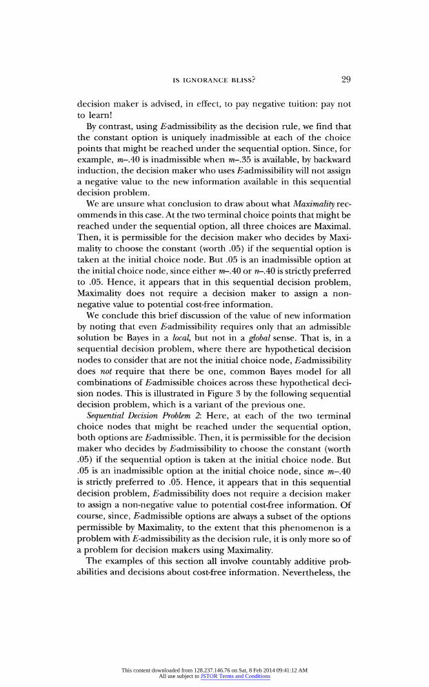
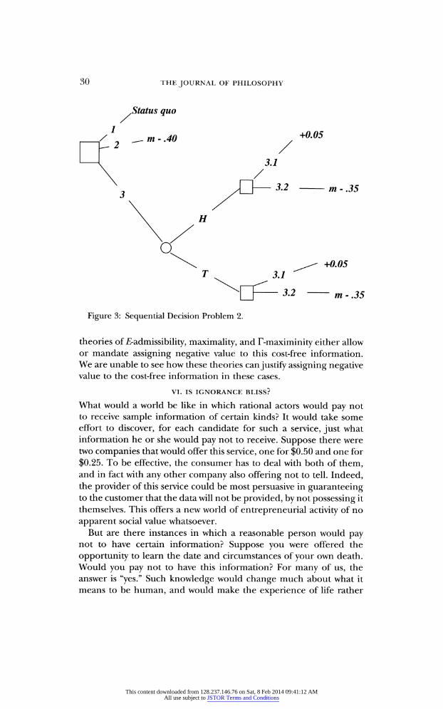
Sequential Decision Problem 2: Here, at each of the two terminal choice nodes that might be reached under the sequential option, both options are ̂ -admissible. Then, it is permissible for the decision maker who decides by E-admissibility to choose the constant (worth .05) if the sequential option is taken at the initial choice node. But .05 is an inadmissible option at the initial choice node, since m-AO is strictly preferred to .05. Hence, it appears that in this sequential decision problem, E-admissibility does not require a decision maker to assign a non-negative value to potential cost-free information. Of course, since, inadmissible options are always a subset of the options permissible by Maximality, to the extent that this phenomenon is a

problem with E-admissibility as the decision rule, it is only more so of a problem for decision makers using Maximality.

The examples of this section all involve countably additive prob abilities and decisions about cost-free information. Nevertheless, the




^Status quo

m-AO +0.05

m - .35

Figure 3: Sequential Decision Problem 2.

theories of E-admissibility, maximality, and r-maximinity either allow or mandate assigning negative value to this cost-free information.

We are unable to see how these theories can justify assigning negative value to the cost-free information in these cases.

VI. IS IGNORANCE BLISS?

What would a world be like in which rational actors would pay not to receive sample information of certain kinds? It would take some effort to discover, for each candidate for such a service, just what information he or she would pay not to receive. Suppose there were two companies that would offer this service, one for $0.50 and one for

$0.25. To be effective, the consumer has to deal with both of them, and in fact with any other company also offering not to tell. Indeed, the provider of this service could be most persuasive in guaranteeing to the customer that the data will not be provided, by not possessing it themselves. This offers a new world of entrepreneurial activity of no

apparent social value whatsoever.

But are there instances in which a reasonable person would pay not to have certain information? Suppose you were offered the

opportunity to learn the date and circumstances of your own death. Would you pay not to have this information? For many of us, the answer is "yes." Such knowledge would change much about what it means to be human, and would make the experience of life rather




different, in a profound way, from all of those who have gone before us. To restructure the way we think about life, and its uncertain time

of end, would be profoundly unsettling and costly, and hence it would be reasonable to pay not to have to undergo that process. On the

other hand, absent professional hitmen, none of us are likely to

receive such an offer.

The issue is more real, however, for those who have to decide whether to be tested for an incurable genetic disease such as Huntington's Disease. This disease generally strikes in people of middle ages, with

neurological and psychological symptoms, ultimately resulting in a

period of helplessness followed by an early death. There are limited treatments that can help to mitigate some of the symptoms, but no cure as yet. Those who are genetic candidates for the disease have a 50%

probability of having the gene. Knowing that one is a candidate, is it

reasonable not to have the test, if it were free? One reason not to have

the test is the response of others to the results: "people lose insurance

and jobs."20 But there are deeper reasons having to do with one's ability to cope and enjoy life that influence this decision. We can not label either decision irrational, given all the implications.

How can we defend the idea of refusing to pay not to see infor mation and yet endorse a decision not to be tested for Huntington's disease by someone who has a parent who had the disease, and hence has a 50% probability of carrying the gene? The insurance issue is

serious, since most life and health insurers ask about known pre

existing conditions. Hence someone who knows they have the gene could easily believe they would be denied coverage on that account.

However, one could imagine a strategy of buying insurance first, and then being tested. Hence, although we take insurance to be an im

portant practical problem, we do not take it as definitive. The real

reasons, we guess, lie deeper. Example 16. (Inherited Disease) There is a certain peace of

mind associated with knowing that, aside from catastrophe, one has the ability to make plans and choices for a relatively long future. There is also value to an individual of having the prospect of making choices and enjoying results in the future. By having a short horizon

placed on our ability to make choices and use our assets, we reduce the overall level of utility. In the terminology of Sen,21 the knowledge

20 Feldman, "One Family's Story: A Quandry over Genetic Testing," Houston Chronicle

(2003), http://www.johnworldpeace.com/e030112e.htm. 21 Sen, "Markets and Freedoms: Achievements and Limitations of the Market

Mechanism in Promoting Individual Freedoms," Oxford Economic Papers, xlv (1993): 519-41, on p. 522.




that one has the disease reduces one's opportunity-freedom. In

symbols, let iff be the knowledge base sequence assuming that I will not learn the results of the test. Let y be the knowledge base

sequence assuming that I will learn (at time t\) whether or not I have the disease. Let X= 1 if I have the disease and X = 0 if not. Let fl = ? X {0,1}, where the second coordinate gives the value of X. Let ?g@, and let ? be a decision that I could make at time t > t\

regardless of the value of X. It might be reasonable that

(19) U((0,\),}pt\d)<U((0,\)9^

for all such 6 and ?. That is, knowing that I have the disease makes

everything worth less than merely supposing that I have the disease, which in turn makes everything worth less than supposing that I do not have the disease, and knowing that I do not have the disease makes everything worth the most. If I am not going to learn the results of the test, the expected utility now of choosing ? at time t is

(20) E[U((0,X)?t,?)] =O.5E[U((0?),yrh?)\X

= O] + 0.5E[U((6,l),y/t,?)\X = 1].

On the other hand, if I am going to learn X in the future, the

expected utility now of choosing ? at time t

(21) O.5?[?/((0,O),yV,<5)IX = 0] + 0.5E[U((6,l),y/t',?) IX = 1].

If the first inequality in (19) is satisfied by a much wider amount than the third inequality and is so satisfied uniformly in 9 and 6, then the

expected utility in (21) will be smaller than the one in (20) for all 5, hence one would prefer not to learn X.

In this connection, it is interesting to note that this is the kind of information the poet Thomas Gray (1747) has in mind. The quote at the start of this paper comes from a poem, "Ode on a Distant

Prospect of Eton College." The first nine stanzas are about the care

less optimism of the students at Eton, and the troubles they are likely to face in life. The concluding tenth stanza reads:

To each his sufferings: all are men

Condemn'd alike to groan? The tender for another's pain, Th' unfeeling for his own.

Yet, ah! why should they know their fate,

Since sorrow never comes too late

And happiness too swiftly flies?

Thought would destroy their Paradise.

No more; where ignorance is bliss

'Tis folly to be wise.




So the question remains of whether it is reasonable to impose the

requirement on a theory of rational decision making that it not

require or permit paying not to see cost-free data. If it is, the only such theory known to us is Bayesian decision theory with a single countably-additive proper prior. Each of the weakenings of this

theory-allowing finitely additive priors, or improper ones, or allowing sets of probabilities with any one of the three decision rules studied here violates this principle.

JOSEPH B. KADANE

MARK SCHERVISH

TEDDY SEIDENFELD

Carnegie Mellon University

APPENDIX

A. 1 Conditioning and Learning. In this appendix we discuss two related matters for understanding how we use conditional probability in connection with changes in evidence:

(i) what conditional probability means in connection with changing bodies of evidence, and

(ii) what it is that is given in a conditional probability.

(i) The first issue about conditional probability arises both with randomized (so-called "mixed") options and in sequential deci sions as we present those in section v. We use coin flips that are

stipulated to be independent of the other events of interest. That

is, for each joint probability distribution we consider, the con

ditional probability for the event of interest given the coin flip equals its unconditional probability. In each example, we argue that, with respect to each probability distribution, given a result of the coin flip, the available options are valued the same as they are valued marginally under that distribution. Such an argument is an

implicit use of conditional probability. There are at least three distinct interpretations of conditional probability, and this appen dix attempts to identify which interpretation we have used in

this paper. Let A and B be events in the algebra over which probability is

defined, and let IA and IB be their indicator functions.22 The con

ditional probability P(A\B), as it relates to degrees of belief

22 What we say here about conditional probability is not restricted to indicator

random variables, which we use for simplicity of exposition only.




and decision making, has been interpreted in at least the following three ways:

(1) Conditional probability and called-off preferences. In the theories of both DeFinetti and Savage, where probability is grounded on un

conditional preferences, conditional probability is reduced to called

off preferences.

(a) Specifically, in DeFinetti, P(A\B) is that prevision p the decision maker offers in order to make the following bet "fair" for all

values of a : \bol(\a ?

p). The bet is "called-off because there is

neither a loss nor a gain if event B fails to occur. DeFinetti shows

that, in order for your called-off previsions to be coherent, that is, immune to a "Book," they must be the values of a (finitely addi

tive) conditional probability function.

(b) In Savage, conditional probability is identified with the decision maker's preferences over pairs of acts that are modified to agree with each other on states that comprise Bc, when B fails. Thus,

these pairs of acts conform to the requirements of being "called

off" in the sense that, for states comprising Bc, the decision

maker of Savage's theory receives the same regardless which

"called-ofF' act is chosen.

It is important to note that in each of these two theories there is no relation between conditional probability and updating beliefs

by new evidence. That is, neither of these theories goes beyond the statics of preference at a time. Neither of these theories offers a

dynamic interpretation of conditional probability that makes it into a learning rule.

(2) Conditional probability and temporal updating. It is a commonplace

interpretation of Bayesian theory to offer the (current) conditional

probability P(A\B) as a "posterior" probability for what the inves

tigator's degree of belief will be in A on the condition that he/she learns that B obtains. Some attempts have been made to extend

deFinetti's static "Book" argument to cover such cases, for example, to make conditional probability into a dynamical, learning rule.

See, for example, Levi,23 for sound reasoning as to why this is an

overreaching of the "Book" argument. Levi refers to the dynamic

interpretation as temporal credal conditionalization.

(3) Conditional probability and hypothetical reasoning. Yet a third sense of conditional probability, the sense used in this paper, is to

understand P(A\B) as the decision maker's current, hypothetical

degrees of belief in A on the condition that he/she were to ac

23Levi, "The Demons of Decision," The Monist, lxx (1987): 193-211.




cept B as true. This sense of conditional probability relates to the

agent's current hypothetical preference were he/she to accept B as true. In this sense, the agent reasons from a hypothetically

augmented body of knowledge that includes B as certain. It differs

from the first sense of P(-\B) in that the space of serious possi

bility is changed by hypothesizing B as a certainty, equating Bc with the impossible event. It differs from the second sense of con

ditional probability in that the decision maker does not predict how he will update his/her degrees of belief at some later time, when B might be accepted as true. (In Levi, this is referred to as

confirmational conditionalization.)

In short, these three senses of conditional probability P(-1B) differ in their consequences for decision making by addressing, respectively:

(1) current, unconditional called-off preferences, called off if Bc obtains;

(2) future, unconditional preferences, upon learning that B obtains;

(3) current, hypothetical preferences obtained by positing that B is true.

Throughout this paper, we use conditional probability to relate to decision making in the third sense, and we use the formalism of se

quential decision making to highlight the difference between the first and third senses of conditional probability. We do not use (or advo

cate) the second sense of conditional probability. (ii) The second matter involving our use of conditional probability

in this paper is made salient in Example 12, the "Taxi Driver" prob lem. There is an important distinction between conditioning on

who-done-it and adding the information to one's knowledge base. Think of D as a random variable taking the value i if the ith charac ter in the mystery committed the crime. Conditioning on D(a>)

= i for i = does not affect my expected utility for any of the decisions that I contemplate choosing in this decision problem. On the other hand, augmenting my current knowledge base either with the information that I know D(a>)

= i or with the information that I will knowZ)(co)

= i before getting to watch the play, has a pronounced effect on the value of going to the play. That knowledge affects my choices in the same, negative way regardless of the value of D that I (will) learn.

Thus, in our use of conditional probability, we need to distin

guish conditioning from learning, and in two ways: From the first issue (i), we use conditional probability to model hypothetical changes in knowledge, rather than requiring conditional probability to be a

learning rule. This takes us beyond merely the use of conditional

probability to model called-off wagers. But it leaves us short of man

dating a single dynamics by which rational agents learn.




From the second issue (ii), we must attend to the event on which we

condition. We recognize that it is not generally the same to condition on E occurring, as it is to condition on the more inclusive event that

you learned that E occurred by some particular method. The dis tinction between conditioning and learning has important con

sequences in the Taxi-Driver Example 12 and in the Inherited Disease

Example 16. We believe that the distinction does not matter in the other examples discussed in this paper.



Journal of Philosophy, Inc. - CMU · Journal of Philosophy, Inc. Is Ignorance Bliss? Author(s): Joseph B. Kadane, Mark Schervish and Teddy Seidenfeld Source: The Journal of Philosophy,

Documents