Joint Calibration for Semantic Segmentation - BMVA · 2 CAESAR ET AL.: JOINT CALIBRATION FOR SEMANTIC SEGMENTATION. Boat, Rock, Sea, Sky. Weakly supervised Fully supervised. Sky,

CAESAR ET AL.: JOINT CALIBRATION FOR SEMANTIC SEGMENTATION 1

Joint Calibration for Semantic SegmentationHolger [email protected]

Jasper [email protected]

Vittorio [email protected]

School of InformaticsUniversity of EdinburghEdinburgh, UK

Abstract

Semantic segmentation is the task of assigning a class-label to each pixel in an im-age. We propose a region-based semantic segmentation framework which handles bothfull and weak supervision, and addresses three common problems: (1) Objects occur atmultiple scales and therefore we should use regions at multiple scales. However, theseregions are overlapping which creates conflicting class predictions at the pixel-level. (2)Class frequencies are highly imbalanced in realistic datasets. (3) Each pixel can onlybe assigned to a single class, which creates competition between classes. We address allthree problems with a joint calibration method which optimizes a multi-class loss definedover the final pixel-level output labeling, as opposed to simply region classification. Ourmethod outperforms the state-of-the-art on the popular SIFT Flow [17] dataset in boththe fully and weakly supervised setting.

1 IntroductionSemantic segmentation is the task of assigning a class label to each pixel in an image (Fig. 1).In the fully supervised setting, we have ground-truth labels for all pixels in the trainingimages. In the weakly supervised setting, class-labels are only given at the image-level. Wetackle both settings in a single framework which builds on region-based classification.

Our framework addresses three important problems common to region-based semanticsegmentation. First of all, objects naturally occur at different scales within an image [3, 35].Performing recognition at a single scale inevitably leads to regions covering only parts ofan object which may have ambiguous appearance, such as wheels or fur, and to regionsstraddling over multiple objects, whose classification is harder due to their mixed appear-ance. Therefore many recent methods operate on pools of regions computed at multiplescales, which have a much better chance of containing some regions covering complete ob-jects [3, 4, 10, 11, 15, 23, 28, 43]. However, this leads to overlapping regions which maylead to conflicting class predictions at the pixel-level. These conflicts need to be properlyresolved.

Secondly, classes are often unbalanced [2, 7, 13, 18, 19, 28, 30, 33, 37, 39, 40, 41]:“cars” and “grass” are frequently found in images while “tricycles” and “gravel” are muchrarer. Due to the nature of most classifiers, without careful consideration these rare classesare largely ignored: even if the class occurs in an image the system will rarely predict it.

c© 2015. The copyright of this document resides with its authors.It may be distributed unchanged freely in print or electronic forms. Pages 29.1-29.13

DOI: https://dx.doi.org/10.5244/C.29.29

2 CAESAR ET AL.: JOINT CALIBRATION FOR SEMANTIC SEGMENTATIONBoat, Rock, Sea, Sky

Weaklysupervised

Fullysupervised

Sky, Building

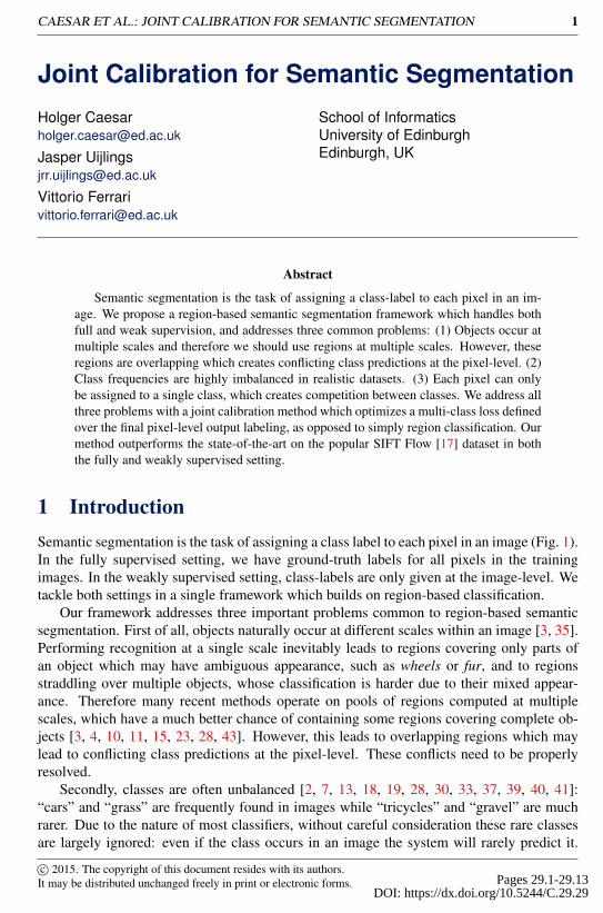
Figure 1: Semantic segmentation is the task of assigning class labels to all pixels in theimage. During training, with full supervision we have ground-truth labels of all pixels. Withweak supervision we only have labels at the image-level.

Since class-frequencies typically follow a power-law distribution, this problem becomes in-creasingly important with the modern trend towards larger datasets with more and moreclasses.

Finally, classes compete: a pixel can only be assigned to a single class (e.g. it can notbelong to both “sky” and “airplane”). To properly resolve such competition, a semanticsegmentation framework should take into account predictions for multiple classes jointly.

In this paper we address these three problems with a joint calibration method over an en-semble of SVMs, where the calibration parameters are optimized over all classes, and for thefinal evaluation criterion, i.e. the accuracy of pixel-level labeling, as opposed to simply re-gion classification. While each SVM is trained for a single class, their joint calibration dealswith the competition between classes. Furthermore, the criterion we optimize for explicitlyaccounts for class imbalance. Finally, competition between overlapping regions is resolvedthrough maximization: each pixel is assigned the highest scoring class over all regions cov-ering it. We jointly calibrate the SVMs for optimal pixel labeling after this maximization,which effectively takes into account conflict resolution between overlapping regions. Resultson the SIFT Flow dataset [17] show that our framework outperforms the state-of-the-art inboth the fully and the weakly supervised setting.

2 Related workEarly works on semantic segmentation used pixel- or patch-based features over which theydefine a Condition Random Field (CRF) [29, 36]. Many modern successful works useregion-level representations, both in the fully supervised [1, 4, 9, 10, 11, 15, 19, 23, 28, 31,32, 34, 41] and weakly supervised [37, 38, 39, 40, 42, 43] settings. A few recent works useCNNs to learn a direct mapping from image to pixel labels [7, 16, 20, 21, 22, 26, 27, 30, 44],although some of them [7, 27] use region-based post-processing to impose label smoothingand to better respect object boundaries. Other recent works use CRFs to refine the CNNpixel-level predictions [5, 16, 20, 26, 44]. In this work we focus on region-based semanticsegmentation, which we discuss in light of the three problems raised in the introduction.

Overlapping regions. Traditionally, semantic segmentation systems use superpixels [1,9, 19, 27, 31, 32, 34, 41], which are non-overlapping regions resulting from a single-scaleoversegmentation. However, appearance-based recognition of superpixels is difficult as theytypically capture only parts of objects, rather than complete objects. Therefore, many recentmethods use overlapping multi-scale regions [3, 4, 10, 11, 15, 23, 43]. However, thesemay lead to conflicting class predictions at the pixel-level. Carreira et al. [4] address thissimply by taking the maximum score over all regions containing a pixel. Both Hariharan etal. [11] and Girshick et al. [10] use non-maximum suppression, which may give problems

CAESAR ET AL.: JOINT CALIBRATION FOR SEMANTIC SEGMENTATION 3

for nearby or interacting objects [15]. Li et al. [15] predict class overlap scores for eachregion at each scale. Then they create superpixels by intersecting all regions. Finally, theyassign overlap scores to these superpixels using maximum composite likelihood (i.e. takingall multi-scale predictions into account). Plath et al. [23] use classification predictions over asegmentation hierarchy to induce label consistency between parent and child regions withina tree-based CRF framework. After solving their CRF formulation, only the smallest regions(i.e. leaf-nodes) are used for class prediction. In the weakly supervised setting, most worksuse superpixels [37, 38, 39, 40] and so do not encounter problems of conflicting predictions.Zhang et al. [42] use overlapping regions to enforce a form of class-label smoothing, butthey all have the same scale. A different Zhang et al. [43] use overlapping region proposalsat multiple scales in a CRF.

Class imbalance. As the PASCAL VOC dataset [6] is relatively balanced, most worksthat experiment on it did not explicitly address this issue [1, 4, 5, 10, 11, 15, 16, 18, 22,23, 26, 44]. On highly imbalanced datasets such as SIFT Flow [17], Barcelona [31] andLM+SUN [33], rare classes pose a challenge. This is observed and addressed by Tighe etal. [33] and Yang et al. [41]: for a test image, only a few training images with similar contextare used to provide class predictions, but for rare classes this constraint is relaxed and moretraining images are used. Vezhnevets et al. [37] balance rare classes by normalizing scoresfor each class to range [0,1]. A few works [19, 39, 40] balance classes by using an inverseclass frequency weighted loss function.

Competing classes. Several works train one-vs-all classifiers separately and resolve label-ing through maximization [4, 10, 11, 15, 19, 22, 23, 33]. This is suboptimal since the scoresof different classes may not be properly calibrated. Instead, Tighe et al. [31, 33] and Yanget al. [41] use Nearest Neighbor classification which is inherently multi-class. In the weaklysupervised setting appearance models are typically trained in isolation and remain uncali-brated [37, 37, 39, 40, 42]. To the best of our knowledge, Boix et al. [1] is the only work insemantic segmentation to perform joint calibration of SVMs. While this enables to handlecompeting classes, in their work they use non-overlapping regions. In contrast, in our workwe use overlapping regions where conflicting predictions are resolved through maximiza-tion. In this setting, joint calibration is particularly important, as we will show in Sec. 4. Asanother difference, Boix et al. [1] address only full supervision whereas we address both fulland weak supervision in a unified framework.

3 Method

3.1 ModelWe represent an image by a set of overlapping regions [35] described by CNN features [10](Sec. 3.4). Our semantic segmentation model infers the label op of each pixel p in an image:

op = argmaxc, r3p

σ(wc · xr, ac,bc) (1)

As appearance models, we have a separate linear SVM wc per class c. These SVMs score thefeatures xr of each region r. The scores are calibrated by a sigmoid function σ , with differentparameters ac,bc for each class c. The argmax returns the class c with the highest score overall regions that contain pixel p. This involves maximizing over classes for a region, and overthe regions that contain p.

4 CAESAR ET AL.: JOINT CALIBRATION FOR SEMANTIC SEGMENTATION

During training we find the SVM parameters wc (Sec. 3.2) and calibration parameters acand bc (Sec. 3.3). The training of the calibration parameters takes into account the effectsof the two maximization operations, as they are optimized for the output pixel-level labelingperformance (as opposed to simply accuracy in terms of region classification).

3.2 SVM trainingFully supervised. In this setting we are given ground-truth pixel-level labels for all imagesin the training set (Fig. 1). This leads to a natural subdivision into ground-truth regions, i.e.non-overlapping regions perfectly covering a single class. We use these as positive trainingsamples. However, such idealized samples are rarely encountered at test time since there wehave only imperfect region proposals [35]. Therefore we use as additional positive samplesfor a class all region proposals which overlap heavily with a ground-truth region of thatclass (i.e. Intersection-over-Union greater than 50% [6]). As negative samples, we use allregions from all images that do not contain that class. In the SVM loss function we applyinverse frequency weighting in terms of the number of positive and negative samples.

Weakly supervised. In this setting we are only given image-level labels on the trainingimages (Fig. 1). Hence, we treat region-level labels as latent variables which are updatedusing an alternated optimization process (as in [37, 38, 39, 40, 43]). To initialize the process,we use as positive samples for a class all regions in all images containing it. At each iterationwe alternate between training SVMs based on the current region labeling and updating thelabeling based on the current SVMs (by assigning to each region the label of the highestscoring class). In this process we keep our negative samples constant, i.e. all regions fromall images that do not contain the target class. In the SVM loss function we apply inversefrequency weighting in terms of the number of positive and negative samples.

3.3 Joint CalibrationWe now introduce our joint calibration procedure, which addresses three common problemsin semantic segmentation: (1) conflicting predictions of overlapping regions, (2) class im-balance, and (3) competition between classes.

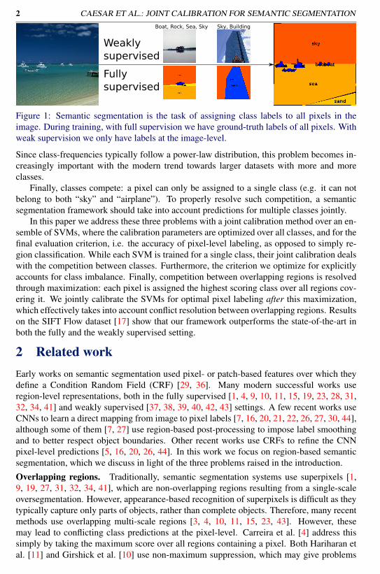
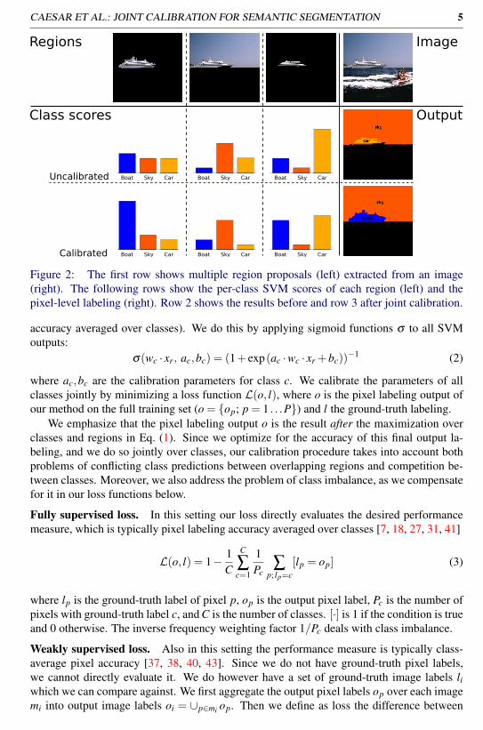
To better understand the problem caused by overlapping regions, consider the exampleof Fig. 2. It shows three overlapping regions, each with different class predictions. The finalgoal of semantic segmentation is to output a pixel-level labeling, which is evaluated in termsof pixel-level accuracy. In our framework we employ a winner-takes all principle: eachpixel takes the class of the highest scored region which contains it. Now, using uncalibratedSVMs is problematic (second row in Fig. 2). SVMs are trained to predict class labels atthe region-level, not the pixel-level. However, different regions have different area, and,most importantly, not all regions contribute all of their area to the final pixel-level labeling:Predictions of small regions may be completely suppressed by bigger regions (e.g. in Fig. 2,row 3, the inner-boat region is suppressed by the prediction of the complete boat). In othercases, bigger regions may be partially overwritten by smaller regions (e.g. in Fig. 2 theboat region partially overwrites the prediction of the larger boat+sky region). Furthermore,the SVMs are trained in a one-vs-all manner and are unaware of other classes. Hence theyare unlikely to properly resolve competition between classes even within a single region.The problems above show that without calibration, the SVMs are optimized for the wrongcriterion. We propose to jointly calibrate SVMs for the correct criterion, which correspondsbetter to the evaluation measure typically used for semantic segmentation (i.e. pixel labeling

CAESAR ET AL.: JOINT CALIBRATION FOR SEMANTIC SEGMENTATION 5

Regions

Class scores

Uncalibrated

Calibrated

Image

Output

Boat Sky Car Boat Sky Car Boat Sky Car

Boat Sky Car Boat Sky Car Boat Sky Car

Figure 2: The first row shows multiple region proposals (left) extracted from an image(right). The following rows show the per-class SVM scores of each region (left) and thepixel-level labeling (right). Row 2 shows the results before and row 3 after joint calibration.

accuracy averaged over classes). We do this by applying sigmoid functions σ to all SVMoutputs:

σ(wc · xr, ac,bc) = (1+ exp(ac ·wc · xr +bc))−1 (2)

where ac,bc are the calibration parameters for class c. We calibrate the parameters of allclasses jointly by minimizing a loss function L(o, l), where o is the pixel labeling output ofour method on the full training set (o = {op; p = 1 . . .P}) and l the ground-truth labeling.

We emphasize that the pixel labeling output o is the result after the maximization overclasses and regions in Eq. (1). Since we optimize for the accuracy of this final output la-beling, and we do so jointly over classes, our calibration procedure takes into account bothproblems of conflicting class predictions between overlapping regions and competition be-tween classes. Moreover, we also address the problem of class imbalance, as we compensatefor it in our loss functions below.

Fully supervised loss. In this setting our loss directly evaluates the desired performancemeasure, which is typically pixel labeling accuracy averaged over classes [7, 18, 27, 31, 41]

L(o, l) = 1− 1C

C

∑c=1

1Pc

∑p; lp=c

[lp = op] (3)

where lp is the ground-truth label of pixel p, op is the output pixel label, Pc is the number ofpixels with ground-truth label c, and C is the number of classes. [·] is 1 if the condition is trueand 0 otherwise. The inverse frequency weighting factor 1/Pc deals with class imbalance.

Weakly supervised loss. Also in this setting the performance measure is typically class-average pixel accuracy [37, 38, 40, 43]. Since we do not have ground-truth pixel labels,we cannot directly evaluate it. We do however have a set of ground-truth image labels liwhich we can compare against. We first aggregate the output pixel labels op over each imagemi into output image labels oi = ∪p∈mi op. Then we define as loss the difference between

6 CAESAR ET AL.: JOINT CALIBRATION FOR SEMANTIC SEGMENTATION

the ground-truth label set li and the output label set oi, measured by the Hamming distancebetween their binary vector representations

L(o, l) =I

∑i=1

C

∑c=1

1Ic|li,c−oi,c| (4)

where li,c = 1 if label c is in li, and 0 otherwise (analog for oi,c). I is the total numberof training images. Ic is the number of images having ground-truth label c, so the loss isweighted by the inverse frequency of class labels, measured at the image-level. Note howalso in this setting the loss looks at performance after the maximization over classes andregions (Eq. (1)).Optimization. We want to minimize our loss functions over the calibration parametersac,bc of all classes. This is hard, because the output pixel labels op depend on these param-eters in a complex manner due to the max over classes and regions in Eq. (1), and becauseof the set-union aggregation in the case of the weakly supervised loss. Therefore, we applyan approximate minimization algorithm based on coordinate descent. Coordinate descent isdifferent from gradient descent in that it can be used on arbitrary loss functions that are notdifferentiable, as it only requires their evaluation for a given setting of parameters.

Coordinate descent iteratively applies line search to optimize the loss over a single pa-rameter at a time, keeping all others fixed. This process cycles through all parameters untilconvergence. As initialization we use constant values (ac =−7, bc = 0). During line searchwe consider 10 equally spaced values (ac in [−12,−2], bc in [−10,10]).

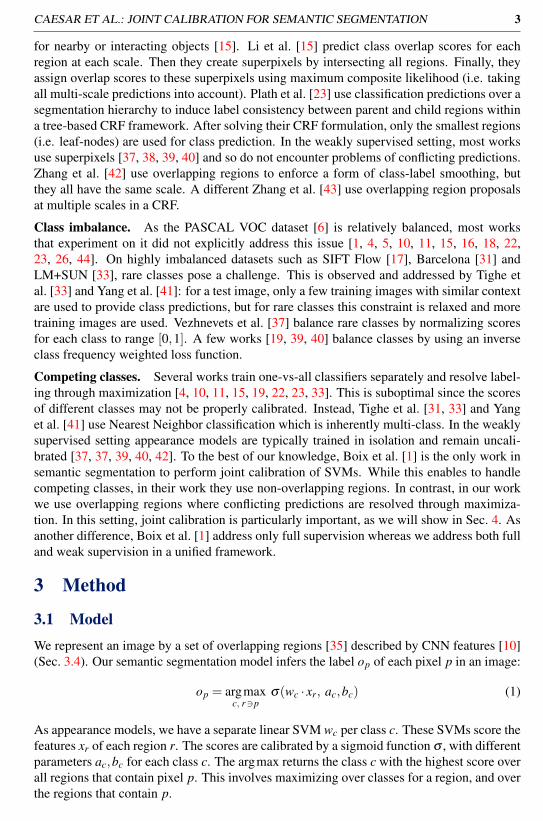
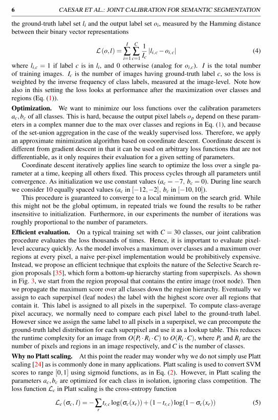
This procedure is guaranteed to converge to a local minimum on the search grid. Whilethis might not be the global optimum, in repeated trials we found the results to be ratherinsensitive to initialization. Furthermore, in our experiments the number of iterations wasroughly proportional to the number of parameters.Efficient evaluation. On a typical training set with C = 30 classes, our joint calibrationprocedure evaluates the loss thousands of times. Hence, it is important to evaluate pixel-level accuracy quickly. As the model involves a maximum over classes and a maximum overregions at every pixel, a naive per-pixel implementation would be prohibitively expensive.Instead, we propose an efficient technique that exploits the nature of the Selective Search re-gion proposals [35], which form a bottom-up hierarchy starting from superpixels. As shownin Fig. 3, we start from the region proposal that contains the entire image (root node). Thenwe propagate the maximum score over all classes down the region hierarchy. Eventually weassign to each superpixel (leaf nodes) the label with the highest score over all regions thatcontain it. This label is assigned to all pixels in the superpixel. To compute class-averagepixel accuracy, we normally need to compare each pixel label to the ground-truth label.However since we assign the same label to all pixels in a superpixel, we can precompute theground-truth label distribution for each superpixel and use it as a lookup table. This reducesthe runtime complexity for an image from O(Pi ·Ri ·C) to O(Ri ·C), where Pi and Ri are thenumber of pixels and regions in an image respectively, and C is the number of classes.Why no Platt scaling. At this point the reader may wonder why we do not simply use Plattscaling [24] as is commonly done in many applications. Platt scaling is used to convert SVMscores to range [0,1] using sigmoid functions, as in Eq. (2). However, in Platt scaling theparameters ac,bc are optimized for each class in isolation, ignoring class competition. Theloss function Lc in Platt scaling is the cross-entropy function

Lc (σc, l) =−∑r

tr,c log(σc(xr))+(1− tr,c) log(1−σc(xr)) (5)

CAESAR ET AL.: JOINT CALIBRATION FOR SEMANTIC SEGMENTATION 7

Building 0.5

Building 0.8

Sky 0.7Building 0.6...

Sky 0.9

Sky 0.8

Input image

Output target

Region hierarchy

Building 0.5

Building 0.8

Building 0.5

Sky 0.8Sky 0.8

Figure 3: Our efficient evaluation algorithm uses the bottom-up structure of Selective Searchregion proposals to simplify the spatial maximization. We start from the root node andpropagate the maximum score with its corresponding label down the tree. We label theimage based on the labels of its superpixels (leaf nodes).

where N+ is the number of positive samples, N− the number of negative samples, and tr,c =N++1N++2 if lr = c or tr,c = 1

N−+2 otherwise; lr is the region-level label. This loss function isinappropriate for semantic segmentation because it is defined in terms of accuracy of trainingsamples, which are regions, rather than in terms of the final pixel-level accuracy. Hence itignores the problem of overlapping regions. There is also no inverse frequency term to dealwith class imbalance. We experimentally compare our method with Platt scaling in Sec. 4.

3.4 Implementation Details

Region proposals. We use Selective Search [35] region proposals using a subset of the“Fast” mode: we keep the similarity measures, but we restrict the scale parameter k to 100and the color-space to RGB. This leads to two bottom-up hierarchies of one initial overseg-mentation [8].

Features. We compute R-CNN features [10] using the Caffe implementation [12] ofAlexNet [14]. Regions are described using all pixels in a tight bounding box, warped toa square image, and fed to the CNN. Since regions are free-form, Girshick et al. [10] ad-ditionally proposes to set pixels not belonging to the region to zero (i.e. not affecting theconvolution). However, in our experiments this did not improve results so we do not use it.

For the weakly supervised setting we use the CNN network pre-trained for image clas-sification on ILSVRC 2012 [25]. For the fully supervised setting we start from this networkand finetune it on the training set of SIFT Flow [17]; the semantic segmentation dataset weexperiment on. For both settings, following [10] we use the output of the 6th layer of thenetwork as features.

SVM training. Like [10] we set the regularization parameter C to a fixed value in allour experiments. The SVMs minimize the L2-loss for region classification. We use hard-negative mining to reduce the memory consumption of our system.

8 CAESAR ET AL.: JOINT CALIBRATION FOR SEMANTIC SEGMENTATION

4 ExperimentsDatasets. We evaluate our method on the challenging SIFT Flow dataset [17]. It consistsof 2488 training and 200 test images, pixel-wise annotated with 33 class labels. The classdistribution is highly imbalanced in terms of overall region count as well as pixel count. Asevaluation measure we use the popular class-average pixel accuracy [7, 18, 21, 28, 31, 34,38, 40, 41, 43]. For both supervision settings we report results on the test set.

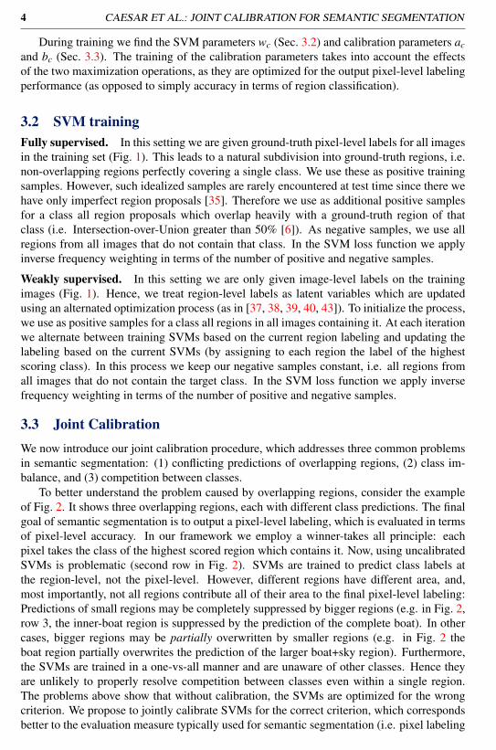
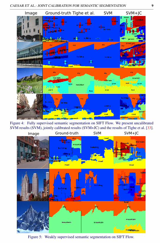
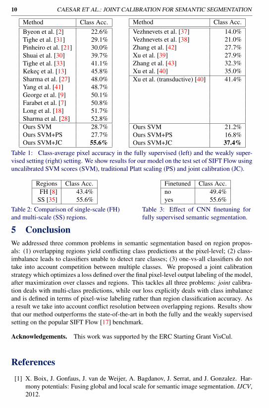
Fully supervised setting. Table 1 evaluates various versions of our model in the fullysupervised setting, and compares to other works on the SIFT Flow dataset. Using uncal-ibrated SVMs, our model achieves a class-average pixel accuracy of 28.7%. If we cali-brate the SVM scores with traditional Platt scaling results do not improve (27.7%). Usingour proposed joint calibration to maximize class-average pixel accuracy improves resultssubstantially to 55.6%. This shows the importance of joint calibration to resolve conflictsbetween overlapping regions at multiple scales, to take into account competition betweenclasses, and generally to optimize a loss mirroring the evaluation measure. Fig. 4 (col-umn “SVM”) shows that larger background regions (i.e. road, building) swallow smallerforeground regions (i.e. person, awning). Many of these small objects become visible af-ter calibration (column “SVM+JC”). This issue is particularly evident when working withoverlapping regions. Consider a large region on a building which contains a awning. As thesurface of the awning is small, the features of the large region will be dominated by the build-ing, leading to strong classification score for the ‘building’ class. When these are higher thanthe classification score for ‘awning’ on the small awning region, the latter gets overwritten.Instead, this problem does not appear when working with superpixels [1]. A superpixel iseither part of the building or part of the awning, so a high scoring awning superpixel cannotbe overwritten by neighboring building superpixels. Hence, joint calibration is particularlyimportant when working with overlapping regions. Our complete model outperforms thestate-of-the-art [28] by 2.8%. For comparison we show the results of [33] (column “Tighe etal.”).

Weakly supervised setting. Table 1 shows results in the weakly supervised setting. Themodel with uncalibrated SVMs achieves an accuracy of 21.2%. Using traditional Platt scal-ing the result is 16.8%, again showing it is not appropriate for semantic segmentation. In-stead, our joint calibration almost doubles accuracy (37.4%). Fig. 5 illustrates the power ofour weakly supervised method. Again rare classes appear only after joint calibration. Ourcomplete model outperforms the state-of-the-art [40] in this setting by 2.4%. Xu et al. [40]additionally report results on the transductive setting (41.4%), where all (unlabeled) test im-ages are given to the algorithm during training.

Region proposals. To demonstrate the importance of multi-scale regions, we also analyzeoversegmentations that do not cover multiple scales. To this end, we keep our frameworkthe same, but instead of Selective Search (SS) [35] region proposals we used a single over-segmentation using the method of Felzenszwalb and Huttenlocher (FH) [8] (for which weoptimized the scale parameter). As Table 2 shows, SS regions outperform FH regions by agood margin of 12.2% in the fully supervised setting. This confirms that overlapping multi-scale regions are superior to non-overlapping oversegmentations.

CNN finetuning. As described in 3.4 we finetune our network for detection in the fullysupervised case. Table 3 shows that this improves results by 6.2% compared to using a CNNtrained only for image classification on ILSVRC 2012.

CAESAR ET AL.: JOINT CALIBRATION FOR SEMANTIC SEGMENTATION 9

Image Ground-truth Tighe et al. SVM SVM+JC

Figure 4: Fully supervised semantic segmentation on SIFT Flow. We present uncalibratedSVM results (SVM), jointly calibrated results (SVM+JC) and the results of Tighe et al. [33].

Image Ground-truth SVM SVM+JC

Figure 5: Weakly supervised semantic segmentation on SIFT Flow.

10 CAESAR ET AL.: JOINT CALIBRATION FOR SEMANTIC SEGMENTATION

Method Class Acc.Byeon et al. [2] 22.6%Tighe et al. [31] 29.1%Pinheiro et al. [21] 30.0%Shuai et al. [30] 39.7%Tighe et al. [33] 41.1%Kekeç et al. [13] 45.8%Sharma et al. [27] 48.0%Yang et al. [41] 48.7%George et al. [9] 50.1%Farabet et al. [7] 50.8%Long et al. [18] 51.7%Sharma et al. [28] 52.8%Ours SVM 28.7%Ours SVM+PS 27.7%Ours SVM+JC 55.6%

Method Class Acc.Vezhnevets et al. [37] 14.0%Vezhnevets et al. [38] 21.0%Zhang et al. [42] 27.7%Xu et al. [39] 27.9%Zhang et al. [43] 32.3%Xu et al. [40] 35.0%Xu et al. (transductive) [40] 41.4%

Ours SVM 21.2%Ours SVM+PS 16.8%Ours SVM+JC 37.4%

Table 1: Class-average pixel accuracy in the fully supervised (left) and the weakly super-vised setting (right) setting. We show results for our model on the test set of SIFT Flow usinguncalibrated SVM scores (SVM), traditional Platt scaling (PS) and joint calibration (JC).

Regions Class Acc.FH [8] 43.4%

SS [35] 55.6%Table 2: Comparison of single-scale (FH)and multi-scale (SS) regions.

Finetuned Class Acc.no 49.4%yes 55.6%

Table 3: Effect of CNN finetuning forfully supervised semantic segmentation.

5 ConclusionWe addressed three common problems in semantic segmentation based on region propos-als: (1) overlapping regions yield conflicting class predictions at the pixel-level; (2) class-imbalance leads to classifiers unable to detect rare classes; (3) one-vs-all classifiers do nottake into account competition between multiple classes. We proposed a joint calibrationstrategy which optimizes a loss defined over the final pixel-level output labeling of the model,after maximization over classes and regions. This tackles all three problems: joint calibra-tion deals with multi-class predictions, while our loss explicitly deals with class imbalanceand is defined in terms of pixel-wise labeling rather than region classification accuracy. Asa result we take into account conflict resolution between overlapping regions. Results showthat our method outperforms the state-of-the-art in both the fully and the weakly supervisedsetting on the popular SIFT Flow [17] benchmark.

Acknowledgements. This work was supported by the ERC Starting Grant VisCul.

References

[1] X. Boix, J. Gonfaus, J. van de Weijer, A. Bagdanov, J. Serrat, and J. Gonzalez. Har-mony potentials: Fusing global and local scale for semantic image segmentation. IJCV,2012.

CAESAR ET AL.: JOINT CALIBRATION FOR SEMANTIC SEGMENTATION 11

[2] W. Byeon, T. M. Breuel, F. Raue, and M. Liwicki. Scene labeling with lstm recurrentneural networks. In CVPR, 2015.

[3] J. Carreira and C. Sminchisescu. Constrained parametric min-cuts for automatic objectsegmentation. In CVPR, 2010.

[4] J. Carreira, R. Caseiro, J. Batista, and C. Sminchisescu. Semantic segmentation withsecond-order pooling. In ECCV, 2012.

[5] L.-C. Chen, G. Papandreou, I. Kokkinos, K. Murphy, and A. Yuille. Semantic imagesegmentation with deep convolutional nets and fully connected crfs. ICLR, 2015.

[6] M. Everingham, L. Van Gool, C. K. I. Williams, J. Winn, and A. Zisserman. ThePASCAL Visual Object Classes (VOC) Challenge. IJCV, 2010.

[7] C. Farabet, C. Couprie, and L. Najman. Learning hierarchical features for scene label-ing. IEEE Trans. on PAMI, 35(8):1915–1929, 2013.

[8] P. Felzenszwalb and D. Huttenlocher. Efficient graph-based image segmentation. IJCV,2004.

[9] M. George. Image parsing with a wide range of classes and scene-level context. InCVPR, 2015.

[10] R. Girshick, J. Donahue, T. Darrell, and J. Malik. Rich feature hierarchies for accurateobject detection and semantic segmentation. In CVPR, 2014.

[11] B. Hariharan, P. Arbeláez, R. Girshick, and J. Malik. Simultaneous detection andsegmentation. In ECCV, 2014.

[12] Y. Jia. Caffe: An open source convolutional architecture for fast feature embedding.http://caffe.berkeleyvision.org/, 2013.

[13] T. Kekeç, R. Emonet, E. Fromont, A. Trémeau, and C. Wolf. Contextually constraineddeep networks for scene labeling. In BMVC, 2014.

[14] A. Krizhevsky, I. Sutskever, and G. E. Hinton. Imagenet classification with deep con-volutional neural networks. In NIPS, 2012.

[15] F. Li, J. Carreira, G. Lebanon, and C. Sminchisescu. Composite statistical inferencefor semantic segmentation. In CVPR, 2013.

[16] G. Lin, C. Shen, I. Reid, and A. van dan Hengel. Efficient piecewise training of deepstructured models for semantic segmentation. arXiv preprint arXiv:1504.01013, 2015.

[17] C. Liu, J. Yuen, and A. Torralba. Nonparametric scene parsing via label transfer. IEEETrans. on PAMI, 33(12):2368–2382, 2011.

[18] J. Long, E. Shelhamer, and T. Darrell. Fully convolutional networks for semantic seg-mentation. In CVPR, 2015.

[19] M. Mostajabi, P. Yadollahpour, and G. Shakhnarovich. Feedforward semantic segmen-tation with zoom-out features. In CVPR, 2015.

12 CAESAR ET AL.: JOINT CALIBRATION FOR SEMANTIC SEGMENTATION

[20] G. Papandreou, L. Chen, K. Murphy, and A. Yuille. Weakly- and semi-supervisedlearning of a deep convolutional network for semantic image segmentation. arXivpreprint arXiv:1502.02734, 2015.

[21] P. Pinheiro and R. Collobert. Recurrent convolutional neural networks for scene pars-ing. In ICML, 2012.

[22] P. Pinheiro and R. Collobert. From image-level to pixel-level labeling with convolu-tional networks. In CVPR, 2015.

[23] N. Plath, M. Toussaint, and S. Nakajima. Multi-class image segmentation using condi-tional random fields and global classification. In ICML, 2009.

[24] J. Platt. Probabilistic outputs for support vector machines and comparisons to regular-ized likelihood methods. Advances in large margin classifiers, 1999.

[25] O. Russakovsky, J. Deng, H. Su, J. Krause, S. Satheesh, S. Ma, Z. Huang, A. Karpa-thy, A. Khosla, M. Bernstein, A. Berg, and L. Fei-Fei. Imagenet large scale visualrecognition challenge. IJCV, 2015. doi: 10.1007/s11263-015-0816-y.

[26] A. Schwing and R. Urtasun. Fully connected deep structured networks. arXiv preprintarXiv:1503.02351, 2015.

[27] A. Sharma, O. Tuzel, and M. Liu. Recursive context propagation network for semanticscene labeling. In NIPS, pages 2447–2455, 2014.

[28] A. Sharma, O. Tuzel, and D. W. Jacobs. Deep hierarchical parsing for semantic seg-mentation. In CVPR, 2015.

[29] J. Shotton, J. Winn, C. Rother, and A. Criminisi. TextonBoost for image understanding:Multi-class object recognition and segmentation by jointly modeling appearance, shapeand context. IJCV, 81(1):2–23, 2009.

[30] B. Shuai, G. Wang, Z. Zuo, B. Wang, and L. Zhao. Integrating parametric and non-parametric models for scene labeling. In CVPR, 2015.

[31] J. Tighe and S. Lazebnik. Superparsing: Scalable nonparametric image parsing withsuperpixels. In ECCV, 2010.

[32] J. Tighe and S. Lazebnik. Understanding scenes on many levels. In ICCV, 2011.

[33] J. Tighe and S. Lazebnik. Finding things: Image parsing with regions and per-exemplardetectors. In CVPR, 2013.

[34] J. Tighe, M. Niethammer, and S. Lazebnik. Scene parsing with object instances andocclusion ordering. In CVPR, 2014.

[35] J. R. R. Uijlings, K. E. A. van de Sande, T. Gevers, and A. W. M. Smeulders. Selectivesearch for object recognition. IJCV, 2013.

[36] J. Verbeek and B. Triggs. Region classification with markov field aspect models. InCVPR, 2007.

CAESAR ET AL.: JOINT CALIBRATION FOR SEMANTIC SEGMENTATION 13

[37] A. Vezhnevets, V. Ferrari, and J. M. Buhmann. Weakly supervised semantic segmenta-tion with multi image model. In ICCV, 2011.

[38] A. Vezhnevets, V. Ferrari, and J. M. Buhmann. Weakly supervised structured outputlearning for semantic segmentation. In CVPR, 2012.

[39] J. Xu, A. Schwing, and R. Urtasun. Tell me what you see and i will show you where itis. In CVPR, 2014.

[40] J. Xu, A. G. Schwing, and R. Urtasun. Learning to segment under various forms ofweak supervision. In CVPR, 2015.

[41] J. Yang, B. Price, S. Cohen, and Y. Ming-Hsuan. Context driven scene parsing withattention to rare classes. In CVPR, 2014.

[42] L. Zhang, Y. Gao, Y. Xia, K. Lu, J. Shen, and R. Ji. Representative discovery ofstructure cues for weakly-supervised image segmentation. In IEEE Transactions onMultimedia, volume 16, pages 470–479, 2014.

[43] W. Zhang, S. Zeng, D. Wang, and X. Xue. Weakly supervised semantic segmentationfor social images. In CVPR, 2015.

[44] S. Zheng, S. Jayasumana, B. Romera-Paredes, V. Vineet, and Z. Su. Conditional ran-dom fields as recurrent neural networks. arXiv preprint arXiv:1502.032405, 2015.