Isogeometric Analysis of the Cahn-Hilliard phase-field model H´ ector G´ omez 1,2 * , Victor M. Calo 1 , Yuri Bazilevs 1 and Thomas J.R. Hughes 1 1: Institute for Computational Engineering and Sciences The University of Texas at Austin 1 University Station, C0200 201 E. 24th Street, Austin, TX 78712 2: University of A Coru˜ na Civil Engineering School Department of Mathematical Methods Campus de Elvi˜ na, 15192, A Coru˜ na Abstract The Cahn-Hilliard equation involves fourth-order spatial derivatives. Finite ele- ment solutions are not common because primal variational formulations of fourth- order operators are well defined and integrable only if the finite element basis func- tions are piecewise smooth and globally C 1 -continuous. There are a very limited number of two-dimensional finite elements possessing C 1 -continuity applicable to complex geometries, but none in three-dimensions. We propose Isogeometric Anal- ysis as a technology that possesses a unique combination of attributes for complex problems involving higher-order differential operators, namely, higher-order accu- racy, robustness, two- and three-dimensional geometric flexibility, compact support, and, most importantly, the possibility of C 1 and higher-order continuity. A NURBS- based variational formulation for the Cahn-Hilliard equation was tested on two- and three-dimensional problems. We present steady state solutions in two-dimensions and, for the first time, in three-dimensions. To achieve these results an adaptive time-stepping method is introduced. We also present a technique for desensitiz- ing calculations to dependence on mesh refinement. This enables the calculation of topologically correct solutions on coarse meshes, opening the way to practical engineering applications of phase-field methodology. Key words: Phase-field, Cahn-Hilliard, Isogeometric Analysis, NURBS, steady state solutions, isoperimetric problem Preprint submitted to Elsevier Science 11 December 2007

Welcome message from author
This document is posted to help you gain knowledge. Please leave a comment to let me know what you think about it! Share it to your friends and learn new things together.
Transcript
Isogeometric Analysis of the Cahn-Hilliard
phase-field model
Hector Gomez1,2 ∗, Victor M. Calo1, Yuri Bazilevs1 andThomas J.R. Hughes1
1: Institute for Computational Engineering and Sciences
The University of Texas at Austin
1 University Station, C0200
201 E. 24th Street, Austin, TX 78712
2: University of A Coruna
Civil Engineering School
Department of Mathematical Methods
Campus de Elvina,
15192, A Coruna
Abstract
The Cahn-Hilliard equation involves fourth-order spatial derivatives. Finite ele-ment solutions are not common because primal variational formulations of fourth-order operators are well defined and integrable only if the finite element basis func-tions are piecewise smooth and globally C1-continuous. There are a very limitednumber of two-dimensional finite elements possessing C1-continuity applicable tocomplex geometries, but none in three-dimensions. We propose Isogeometric Anal-ysis as a technology that possesses a unique combination of attributes for complexproblems involving higher-order differential operators, namely, higher-order accu-racy, robustness, two- and three-dimensional geometric flexibility, compact support,and, most importantly, the possibility of C1 and higher-order continuity. A NURBS-based variational formulation for the Cahn-Hilliard equation was tested on two- andthree-dimensional problems. We present steady state solutions in two-dimensionsand, for the first time, in three-dimensions. To achieve these results an adaptivetime-stepping method is introduced. We also present a technique for desensitiz-ing calculations to dependence on mesh refinement. This enables the calculationof topologically correct solutions on coarse meshes, opening the way to practicalengineering applications of phase-field methodology.
Key words: Phase-field, Cahn-Hilliard, Isogeometric Analysis, NURBS, steadystate solutions, isoperimetric problem
Preprint submitted to Elsevier Science 11 December 2007
Report Documentation Page Form ApprovedOMB No. 0704-0188
Public reporting burden for the collection of information is estimated to average 1 hour per response, including the time for reviewing instructions, searching existing data sources, gathering andmaintaining the data needed, and completing and reviewing the collection of information. Send comments regarding this burden estimate or any other aspect of this collection of information,including suggestions for reducing this burden, to Washington Headquarters Services, Directorate for Information Operations and Reports, 1215 Jefferson Davis Highway, Suite 1204, ArlingtonVA 22202-4302. Respondents should be aware that notwithstanding any other provision of law, no person shall be subject to a penalty for failing to comply with a collection of information if itdoes not display a currently valid OMB control number.
1. REPORT DATE DEC 2007 2. REPORT TYPE
3. DATES COVERED 00-00-2007 to 00-00-2007
4. TITLE AND SUBTITLE Isogeometric Analysis of the Cahn-Hilliard phase-field model
5a. CONTRACT NUMBER
5b. GRANT NUMBER
5c. PROGRAM ELEMENT NUMBER
6. AUTHOR(S) 5d. PROJECT NUMBER
5e. TASK NUMBER
5f. WORK UNIT NUMBER
7. PERFORMING ORGANIZATION NAME(S) AND ADDRESS(ES) University of Texas at Austin,Institute for Computational Engineeringand Sciences,1 University Station,Austin,TX,78712
8. PERFORMING ORGANIZATIONREPORT NUMBER
9. SPONSORING/MONITORING AGENCY NAME(S) AND ADDRESS(ES) 10. SPONSOR/MONITOR’S ACRONYM(S)
11. SPONSOR/MONITOR’S REPORT NUMBER(S)
12. DISTRIBUTION/AVAILABILITY STATEMENT Approved for public release; distribution unlimited
13. SUPPLEMENTARY NOTES
14. ABSTRACT The Cahn-Hilliard equation involves fourth-order spatial derivatives. Finite element solutions are notcommon because primal variational formulations of fourth-order operators are well defined and integrableonly if the finite element basis functions are piecewise smooth and globally C1-continuous. There are a verylimited number of two-dimensional finite elements possessing C1-continuity applicable to complexgeometries, but none in three-dimensions. We propose Isogeometric Analysis as a technology that possessesa unique combination of attributes for complex problems involving higher-order differential operators,namely, higher-order accuracy, robustness, two- and three-dimensional geometric exibility, compactsupport, and, most importantly, the possibility of C1 and higher-order continuity. A NURBS-basedvariational formulation for the Cahn-Hilliard equation was tested on two- and three-dimensionalproblems. We present steady state solutions in two-dimensions and, for the first time, in three-dimensions.To achieve these results an adaptive time-stepping method is introduced. We also present a technique fordesensitizing calculations to dependence on mesh refinement. This enables the calculation of topologicallycorrect solutions on coarse meshes, opening the way to practical engineering applications of phase-field methodology.
15. SUBJECT TERMS
16. SECURITY CLASSIFICATION OF: 17. LIMITATION OF ABSTRACT Same as
Report (SAR)
18. NUMBEROF PAGES
46
19a. NAME OFRESPONSIBLE PERSON
a. REPORT unclassified
b. ABSTRACT unclassified
c. THIS PAGE unclassified
Standard Form 298 (Rev. 8-98) Prescribed by ANSI Std Z39-18
1 Introduction
1.1 Phase transition phenomena: the phase-field approach
Two different approaches have been used to describe phase transition phenom-ena: sharp-interface models and phase-field (diffuse-interface) models. Tradi-tionally, the evolution of interfaces, such as the liquid-solid interface, has beenmodeled using sharp-interface models [37,70]. This entails the resolution of amoving boundary problem. Thus, the partial differential equations that holdin each phase (for instance, describing mass conservation and heat diffusion)have to be solved. These equations are coupled by boundary conditions onthe interface, such as the Stefan condition demanding energy balance and theGibbs-Thomson equation [6,21,59]. Across the sharp interface, certain quan-tities (e.g., the heat flux, the concentration or the energy) may suffer jumpdiscontinuities. The free-boundary (sharp-interface) description has been asuccessful model in a wide range of situations, but it also presents complica-tions from the physical [2] and computational [15] points of view.
Phase-field models provide an alternative description for phase-transition phe-nomena. The phase-field method has been used to model foams [32], describesolidification processes [10,63], dendritic flow [49,53], microstructure evolutionin solids [34], and liquid-liquid interfaces [61]. For recent reviews of phase-fieldmethods the reader is referred to [16,30].
The key idea in phase-field models is to replace sharp interfaces by thin tran-sition regions where the interfacial forces are smoothly distributed. Explicitfront tracking is avoided by using smooth continuous variables locating grainsor phase boundaries.
Phase-field models can be derived from classical irreversible thermodynam-ics [40]. Utilizing asymptotic expansions for vanishing interface thickness, itcan be shown that classical sharp-interface models, including physical laws atinterfaces and multiple junctions, are recovered [36,38]. In order to capturethe physics of the problem, the transition regions (diffuse interfaces) in thephase-field models have to be extremely thin.
The use of diffuse-interface models to describe interfacial phenomena datesback to Korteweg [55] (1901), Cahn and Hilliard [12] (1958), Landau andGinzburg [56] (1965) and van der Waals [72] (1979).
The Cahn-Hilliard phase-field model is normally used to simulate phase seg-
∗ Corresponding authorEmail address: [email protected] (Hector Gomez1,2).
2
regation of a binary alloy system, but many other applications, such as, imageprocessing [23], planet formation [69] and cancer growth [33] are encounteredin the literature.
1.2 Numerical methods for the Cahn-Hilliard phase-field model
1.2.1 Spatial discretization
The Cahn-Hilliard equation involves fourth-order spatial partial-differentialoperators. Traditional numerical methodologies for dealing with higher-orderoperators on very simple geometries include finite differences (see applica-tions to the Cahn-Hilliard equation in [35,67]) and spectral approximations(solutions to the Cahn-Hilliard equation can be found in [58,60,76,77]). Inreal-world engineering applications, simple geometries are not very relevant,and therefore more geometrically flexible technologies need to be utilized. Itis primarily this reason that has led to the finite element method being themost widely used methodology in engineering analysis. The primary strengthof finite element methods has been in the realm of second-order spatial op-erators. The reason for this is variational formulations of second-order opera-tors involve integration of products of first-derivatives. These are well definedand integrable if the finite element basis functions are piecewise smooth andglobally C0-continuous, which is precisely the case for standard finite elementfunctions. On the other hand, fourth-order operators necessitate basis func-tions that are piecewise smooth and globally C1-continuous. There are a verylimited number of two-dimensional finite elements possessing C1-continuityapplicable to complex geometries, but none in three-dimensions (see [66] for arecent study on C1-continuous finite elements). As a result, a number of differ-ent procedures have been employed over the years to deal with higher-orderoperators. All represent theoretical and computational complexities of one de-gree or another. Unfortunately, it may be said that after 50 years of finiteelement research, no general, elegant and efficient solution of the higher-orderoperator problem exists.
For the above reasons, finite element solutions to the Cahn-Hilliard equationare not common. The most common way to solve this equation in finite ele-ment analysis has been with mixed methods [4,5,9,24–26,31] rather than theuse of C1-continuous function spaces [28]. Recently, a discontinuous Galerkin(DG) formulation has been proposed (see [75]). All of these methods lead tothe introduction of extra degrees of freedom in addition to primal unknowns.As a consequence, an alternative approach is desirable. Perhaps, the most ef-ficient procedure developed to date is the so-called continuous/discontinuousGalerkin (CDG) method [29,74]. In this method, standard C0-continuous finiteelement basis functions are used in conjunction with a variational formulation
3
that maintains C1-continuity weakly through use of discontinuous Galerkinoperators on derivatives. This eliminates extra degrees of freedom at the priceof the inclusion of the discontinuous Galerkin operators which change the datastructure from the normal one based solely on element interior contributions toone in which element edge or surface contributions are additionally required.Nevertheless, due to the reduction in degrees of freedom, this method seemsto have the advantage over others previously proposed.
Recently, a new methodology, Isogeometric Analysis, has been introduced thatis based on recent developments in computational geometry and computeraided design (CAD) [46]. Isogeometric analysis is a generalization of finite el-ement analysis possessing several advantages: 1) It enables precise geometricdefinition of complex engineering designs thus reducing errors caused by low-order, faceted geometric approximation of finite elements. 2) It simplifies meshrefinement because even the coarsest model precisely represents the geometry.Thus, no link is necessary to the CAD geometry in order to refine the mesh,in contrast with the finite element method, in which each mesh represents adifferent approximation of the geometry. 3) It holds promise to simplify themesh generation process, currently the most significant component of analysismodel generation, and a major bottleneck in the overall engineering process.4) The k-refinement process, unique to isogeometric analysis among geomet-rically flexible methodologies, has been shown to possess significant accuracyand robustness properties, compared with the usual p-refinement procedureutilized in finite element methods [3,20].
k-refinement is a procedure in which the order of approximation is increased,as in the p-method, but continuity (i.e., smoothness) is likewise increased,in contrast to the p-method. Isogeometric analysis, thus, presents a uniquecombination of attributes that can be exploited on problems involving higher-order differential operators, namely, higher-order accuracy, robustness, two-and three-dimensional geometric flexibility, compact support, and, most im-portantly, C1 and higher-order continuity. In addition, higher-order continuityis achieved without introducing extra degrees of freedom. These propertiesopen the way to application to phase-field models. Herein, we report our initialefforts to simulate higher-order operators using isogeometric analysis. Higher-order operators are encountered in biomedical applications and in many areasof engineering, such as, for example, liquid-liquid flows, liquid-vapor flows,emulsification, cancer growth, rotation-free thin shell theory, strain-gradientelastic and inelastic material models, and dynamic crack propagation, etc. Thesimplicity of isogeometric analysis compared with many procedures that havebeen published in the literature is noteworthy. We believe it may prove aneffective procedure for solving problems of these kinds on complex geometries.
4
1.2.2 Time discretization
The time integration of the Cahn-Hilliard equation is not trivial. The non-linear fourth-order term imposes severe time-step size restrictions for explicitmethods, thus mandating the use of implicit or (at least) semi-implicit algo-rithms. Under the non-realistic hypothesis that assumes the mobility to beconstant, the fourth-order term of the Cahn-Hilliard equation becomes linear.One can take advantage of this fact by using a semi-implicit time integratorthat treats the fourth-order term implicitly, while the non-linear second-orderterm is treated explicitly [77,43]. This technique allows a somewhat larger timestep than explicit methods while avoiding the use of nonlinear solvers. How-ever, in this paper we are interested in the thermodynamically relevant case,where the mobility depends on concentration and the fourth-order term is nolonger linear. As a consequence, we will use a fully implicit time integrationscheme which requires the use of a nonlinear solver.
Adaptive time stepping is of prime importance because the dynamic responseof the Cahn-Hilliard equation intermittently experiences fast variations intime. The usual approach presented in the literature for simplified versionsof the Cahn-Hilliard equation has been to use a few (2 or 3) different time-step sizes during the simulation [14]. These time steps are not selected bymeans of accuracy criteria, but by using approximate theories of the late-time behavior of the Cahn-Hilliard equation [73]. In this paper we propose anadaptive-in-time method where the time step is selected by using an accuracycriterion. This allows us to reduce the compute time by factors of hundredswhile ensuring that sufficient time accuracy is achieved. (Another approachthat has been used in the literature to speed up the solution is the use ofmultigrid methods [51,52], which is not pursued in this work.)
2 The strong form of the Cahn-Hilliard equation
Let Ω ⊂ Rd be an open set, where d = 2 or 3. The boundary of Ω, assumed
sufficiently smooth, is denoted Γ. The unit outward normal to Γ is denotedn. We assume the boundary Γ is composed of two complementary parts, Γ =Γg ∪ Γs. A binary mixture is contained in Ω and c denotes the concentrationof one of its components. The evolution of the mixture is assumed governedby the Cahn-Hilliard equation. In strong form, the problem can be stated as:find c : Ω× (0, T ) 7→ R such that
5
∂c
∂t= ∇ · (Mc∇(µc − λ∆c)) in Ω× (0, T ), (1.1)
c = g on Γg × (0, T ), (1.2)
Mc∇(µc − λ∆c) · n = s on Γs × (0, T ), (1.3)
Mcλ∇c ·n = 0 on Γ× (0, T ), (1.4)
c(x, t) = c0(x) in Ω. (1.5)
where Mc is the mobility, µc represents the chemical potential of a regularsolution in the absence of phase interfaces and λ is a positive constant suchthat
√λ represents a length scale of the problem. This length scale is related
to the thickness of the interfaces that represent the transition between the twophases.
Remarks:
(1) In most of the existing analytic studies, as well as numerical simulations,the mobility is assumed to be constant. However, according to thermo-dynamics [11], it should depend on the mixture composition. This depen-dence might produce quite important changes of the coarsening kinetics.In this paper we consider the commonly adopted relationship
Mc = Dc(1− c) (2)
in which D is a positive constant which has dimensions of diffusivity, thatis, length2/time. This relationship appeared in the original derivation ofthe Cahn-Hilliard equation [11] and is commonly referred to as degeneratemobility, as pure phases have no mobility. We observe that relation (2)restricts the diffusion process primarily to the interfacial zones, whichis precisely what happens in many physical situations where movementof atoms is confined to the interfacial region [11]. The reader is referredto the paper by Elliott and Garcke [27] for a proof of the existence ofweak solutions of the Cahn-Hilliard equation with degenerate mobility.Further information about the regularity of the solutions can be found in[50]. Numerical simulations of the Cahn-Hilliard equation with degeneratemobility are reported on in [4,74,75].
(2) The function µc is a highly nonlinear function of the concentration rep-resenting the chemical potential of a uniform solution [12]. It is usuallyapproximated by a polynomial of degree three. In this paper we considerthe thermodynamically consistent function, namely
µc =1
2θlog
c
1− c+ 1− 2c (3)
where θ = Tc/T is a dimensionless number which represents the ratiobetween the critical temperature Tc (the temperature at which the two
6
phases attain the same composition) and the absolute temperature T .
2.1 The energy functional for the Cahn-Hilliard equation
An important feature of the Cahn-Hilliard model is the existence of an energyfunctional given by the Ginzburg-Landau free energy, namely
E(c) =∫
Ω(Ψc + Ψs) dx (4)
where Ψc is the chemical free energy and Ψs a surface free energy term. Ac-cording to the original model of Cahn and Hilliard [12,13], the surface freeenergy is given by
Ψs = Nω1
2λ||∇c||2 (5)
while the chemical free energy takes the form
Ψc = NkT (c log c + (1− c) log(1− c)) + Nωc(1− c) (6)
where N is the number of molecules per unit volume, k is Boltzmann’s constantand ω is an interaction energy, which, for a system with a miscibility gap, ispositive and is related to the critical temperature by
ω = 2kTc (7)
For θ = Tc/T > 1, the chemical free energy is non-convex, with two wells,which drive phase segregation into the two binodal points (values of c thatminimize the chemical free energy). For θ ≤ 1 it has a single well and admitsa single phase only.
The chemical potential µc is given by µc = Ψc′/(Nω), where Ψc′ is the deriva-tive of Ψc with respect to c. Due to the complexity of the function Ψc, somesimpler approximations are normally employed. In particular, a polynomial ofdegree four has been used to approximate the chemical free energy in most ana-lytic studies and numerical simulations . The paper by Debussche and Detorri[22] (from the analytic point of view) and the papers by Wells et al. [74],Copetti et al. [19] and Xia et al. [75] (from the numerical point of view) dealwith the issue of logarithmic free energy. In the present work we will use thelogarithmic function given by (6).
Remarks:
(1) According to the Cahn-Hilliard model, the concentration is driven to thebinodal points (those values of c that minimize the chemical free energy)and not to the pure phases.
7
(2) The energy functional given by (4) constitutes a Lyapunov functionalsince some simple manipulations lead to the inequality
dE
dt= −
∫
Ω∇(−λ∆c + µc)Mc∇(−λ∆c + µc)dx ≤ 0 (8)
where E is a real-valued function defined as E(t) = E(c(·, t)).
2.2 Dimensionless form of the Cahn-Hilliard equation
In the numerical examples presented in this paper, we will use a dimensionlessform of the Cahn-Hilliard equation. To derive the dimensionless equation, weintroduce non-dimensional space and time coordinates
x? = x/L0, t? = t/T0 (9)
where L0 is a representative length scale and T0 = L40/(Dλ). In the dimen-
sionless coordinates, the Cahn-Hilliard equation becomes
∂c
∂t?= ∇? · (M?
c∇?(µ?c −∆?c)) (10)
where M?c = c(1− c) and µ?
c = µcL20/λ.
We will also make use of the dimensionless Ginzburg-Landau free energy givenby
E? =∫
Ω?
(
c log c + (1− c) log(1− c) + 2θc(1− c) +θ
3α||∇?c||2
)
dx? (11)
where E? = E(NkTL30)
−1 and
α =L2
0
3λ(12)
is a dimensionless number related to the inverse of the thickness of the inter-faces. The thickness of the interface is inversely proportional to α1/2.
Following [74], we will take the value θ = 3/2 for the temperatures ratio (thiscorresponds to a physically relevant case). Therefore, the value of α completelycharacterizes our solutions.
Remark:
In what follows we will use the dimensionless form of the Cahn-Hilliard equa-tion. For notational simplicity, we will omit the superscript stars henceforth.
8
3 Numerical formulation
3.1 Continuous problem in the weak form
We begin by considering a weak form for the Cahn-Hilliard equation. Let Vdenote the trial solution and weighting functions spaces, which are assumedto be identical. At this point we consider periodic boundary conditions inall directions. Therefore, the variational formulation is stated as follows: findc ∈ V such that ∀w ∈ V,
B(w, c) = 0 (13)
where
B(w, c) =
(
w,∂c
∂t
)
Ω
+ (∇w, Mc∇µc +∇Mc∆c)Ω + (∆w, Mc∆c)Ω (14)
being (·, ·)Ω the L2 inner product with respect to the domain Ω. The spaceV = H2 is a Sobolev space of square integrable functions with square integrablefirst and second derivatives.
The repeated integration by parts of equation (14) under the assumptionsof periodic boundary conditions and sufficient regularity leads to the Euler-Lagrange form of (14):
(
w,∂c
∂t−∇ · (Mc∇(µc −∆c))
)
Ω= 0 (15)
which implies the weak satisfaction of equation (10).
We refer to this formulation as the primal variational formulation.
3.2 The semidiscrete formulation
For the space discretization of (13) we make use of the Galerkin method. Weapproximate (13) by the following variational problem over the finite elementspaces: find ch ∈ Vh ⊂ V such that ∀wh ∈ Vh ⊂ V
B(wh, ch) = 0 (16)
where wh and ch are defined as
9
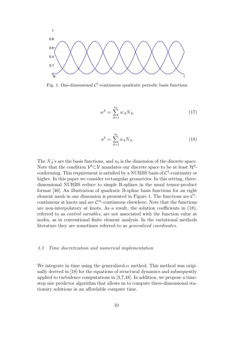
Fig. 1. One-dimensional C1-continuous quadratic periodic basis functions
wh =nb∑
A=1
wANA, (17)
uh =nb∑
A=1
uANA. (18)
The NA’s are the basis functions, and nb is the dimension of the discrete space.Note that the condition Vh⊂V mandates our discrete space to be at least H2-conforming. This requirement is satisfied by a NURBS basis of C1-continuity orhigher. In this paper we consider rectangular geometries. In this setting, three-dimensional NURBS reduce to simple B-splines in the usual tensor-productformat [46]. An illustration of quadratic B-spline basis functions for an eightelement mesh in one dimension is presented in Figure 1. The functions are C1-continuous at knots and are C∞-continuous elsewhere. Note that the functionsare non-interpolatory at knots. As a result, the solution coefficients in (18),referred to as control variables, are not associated with the function value atnodes, as in conventional finite element analysis. In the variational methodsliterature they are sometimes referred to as generalized coordinates.
3.3 Time discretization and numerical implementation
We integrate in time using the generalized-α method. This method was origi-nally derived in [18] for the equations of structural dynamics and subsequentlyapplied to turbulence computations in [3,7,48]. In addition, we propose a time-step size predictor algorithm that allows us to compute three-dimensional sta-tionary solutions in an affordable compute time.
10
3.3.1 Time-stepping scheme
Let C and C denote the vector of degrees of freedom of concentration andconcentration time derivative, respectively. We define the residual vector as
R = RA (19.1)
RA = B(NA, ch) (19.2)
The algorithm can be stated as: given Cn, Cn and ∆tn = tn+1−tn, find Cn+1,Cn+1, Cn+αm
, Cn+αfsuch that
R(Cn+αm, Cn+αf
) = 0, (20.1)
Cn+1 = Cn + ∆tnCn + γ∆tn(Cn+1 − Cn), (20.2)
Cn+αm= Cn + αm(Cn+1 − Cn), (20.3)
Cn+αf= Cn + αf(Cn+1 −Cn). (20.4)
where ∆tn is the current time-step size and αm, αf and γ are real-valuedparameters that define the method. Parameters αm, αf and γ are selectedbased on considerations of accuracy and stability. Taking αm = αf = γ =1, the first order backward Euler method is obtained. Jansen, Whiting andHulbert proved in [48] that, for a linear model problem, second-order accuracyin time is achieved if
γ =1
2+ αm − αf (21)
and unconditional stability is attained if
αm ≥ αf ≥ 1/2 (22)
Parameters αm, αf can be parameterized in terms of ρ∞, the spectral radiusof the amplification matrix as ∆t → ∞, which controls high-frequency dissi-pation [45]:
αm =1
2
(
3− ρ∞
1 + ρ∞
)
, αf =1
1 + ρ∞
(23)
11
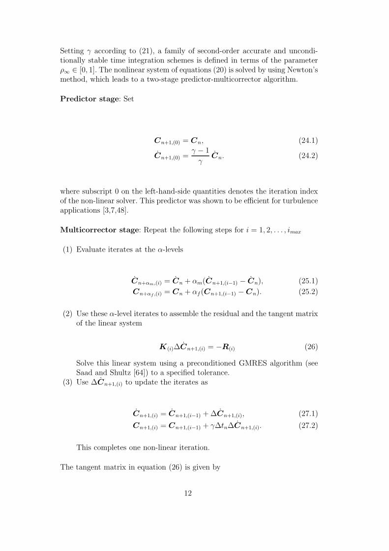
Setting γ according to (21), a family of second-order accurate and uncondi-tionally stable time integration schemes is defined in terms of the parameterρ∞ ∈ [0, 1]. The nonlinear system of equations (20) is solved by using Newton’smethod, which leads to a two-stage predictor-multicorrector algorithm.
Predictor stage: Set
Cn+1,(0) = Cn, (24.1)
Cn+1,(0) =γ − 1
γCn. (24.2)
where subscript 0 on the left-hand-side quantities denotes the iteration indexof the non-linear solver. This predictor was shown to be efficient for turbulenceapplications [3,7,48].
Multicorrector stage: Repeat the following steps for i = 1, 2, . . . , imax
(1) Evaluate iterates at the α-levels
Cn+αm,(i) = Cn + αm(Cn+1,(i−1) − Cn), (25.1)
Cn+αf ,(i) = Cn + αf (Cn+1,(i−1) −Cn). (25.2)
(2) Use these α-level iterates to assemble the residual and the tangent matrixof the linear system
K(i)∆Cn+1,(i) = −R(i) (26)
Solve this linear system using a preconditioned GMRES algorithm (seeSaad and Shultz [64]) to a specified tolerance.
(3) Use ∆Cn+1,(i) to update the iterates as
Cn+1,(i) = Cn+1,(i−1) + ∆Cn+1,(i), (27.1)
Cn+1,(i) = Cn+1,(i−1) + γ∆tn∆Cn+1,(i). (27.2)
This completes one non-linear iteration.
The tangent matrix in equation (26) is given by
12
K =∂R(Cn+αm
, Cn+αf)
∂Cn+αm
∂Cn+αm
∂Cn+1
+∂R(Cn+αm
, Cn+αf)
∂Cn+αf
∂Cn+αf
∂Cn+1
= αm
∂R(Cn+αm, Cn+αf
)
∂Cn+αm
+ αfγ∆tn∂R(Cn+αm
, Cn+αf)
∂Cn+αf
(28)
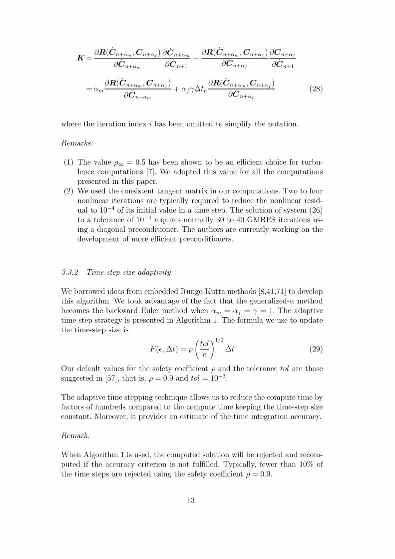
where the iteration index i has been omitted to simplify the notation.
Remarks:
(1) The value ρ∞ = 0.5 has been shown to be an efficient choice for turbu-lence computations [7]. We adopted this value for all the computationspresented in this paper.
(2) We used the consistent tangent matrix in our computations. Two to fournonlinear iterations are typically required to reduce the nonlinear resid-ual to 10−4 of its initial value in a time step. The solution of system (26)to a tolerance of 10−4 requires normally 30 to 40 GMRES iterations us-ing a diagonal preconditioner. The authors are currently working on thedevelopment of more efficient preconditioners.
3.3.2 Time-step size adaptivity
We borrowed ideas from embedded Runge-Kutta methods [8,41,71] to developthis algorithm. We took advantage of the fact that the generalized-α methodbecomes the backward Euler method when αm = αf = γ = 1. The adaptivetime step strategy is presented in Algorithm 1. The formula we use to updatethe time-step size is
F (e, ∆t) = ρ
(
tol
e
)1/2
∆t (29)
Our default values for the safety coefficient ρ and the tolerance tol are thosesuggested in [57], that is, ρ = 0.9 and tol = 10−3.
The adaptive time stepping technique allows us to reduce the compute time byfactors of hundreds compared to the compute time keeping the time-step sizeconstant. Moreover, it provides an estimate of the time integration accuracy.
Remark:
When Algorithm 1 is used, the computed solution will be rejected and recom-puted if the accuracy criterion is not fulfilled. Typically, fewer than 10% ofthe time steps are rejected using the safety coefficient ρ = 0.9.
13
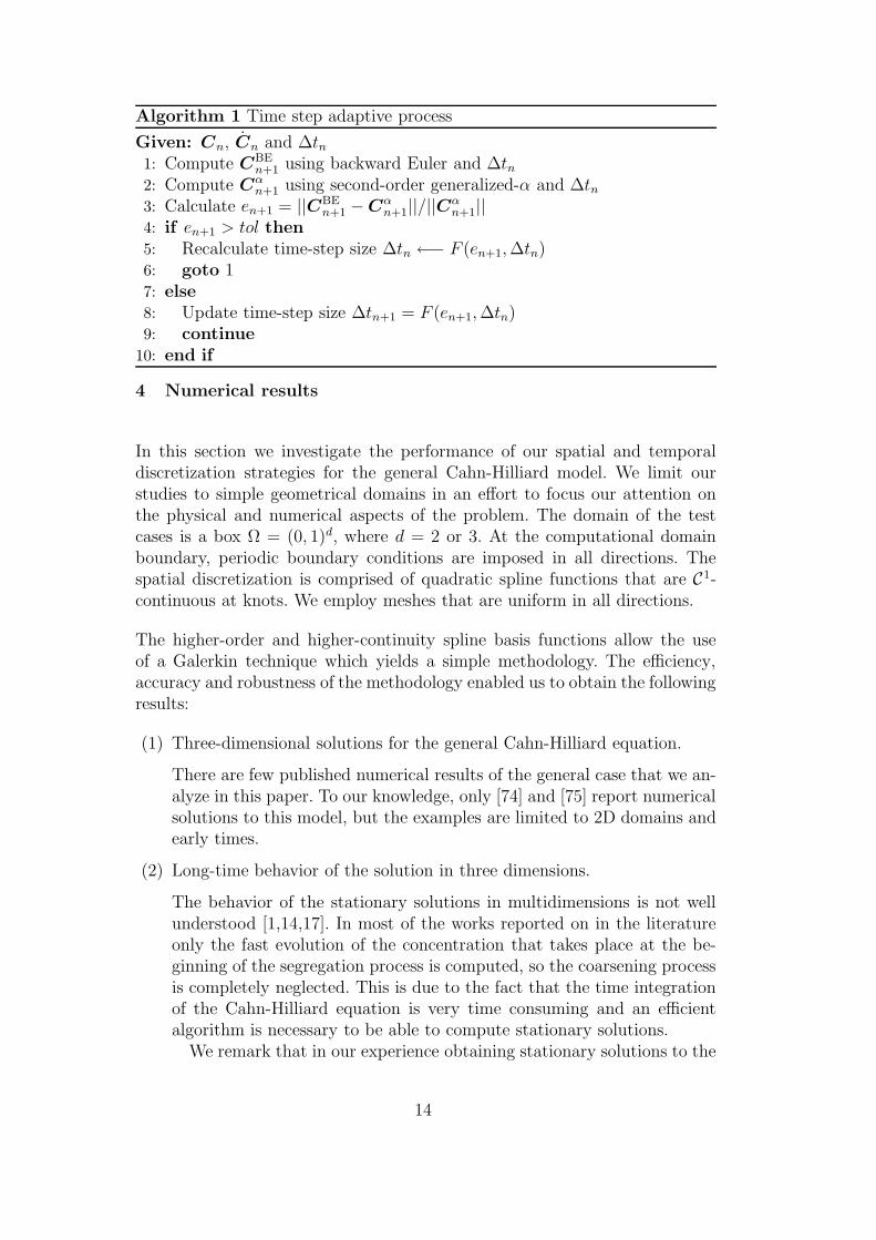
Algorithm 1 Time step adaptive process
Given: Cn, Cn and ∆tn1: Compute C
BEn+1 using backward Euler and ∆tn
2: Compute Cαn+1 using second-order generalized-α and ∆tn
3: Calculate en+1 = ||CBEn+1 −C
αn+1||/||Cα
n+1||4: if en+1 > tol then
5: Recalculate time-step size ∆tn ←− F (en+1, ∆tn)6: goto 17: else
8: Update time-step size ∆tn+1 = F (en+1, ∆tn)9: continue
10: end if
4 Numerical results
In this section we investigate the performance of our spatial and temporaldiscretization strategies for the general Cahn-Hilliard model. We limit ourstudies to simple geometrical domains in an effort to focus our attention onthe physical and numerical aspects of the problem. The domain of the testcases is a box Ω = (0, 1)d, where d = 2 or 3. At the computational domainboundary, periodic boundary conditions are imposed in all directions. Thespatial discretization is comprised of quadratic spline functions that are C1-continuous at knots. We employ meshes that are uniform in all directions.
The higher-order and higher-continuity spline basis functions allow the useof a Galerkin technique which yields a simple methodology. The efficiency,accuracy and robustness of the methodology enabled us to obtain the followingresults:
(1) Three-dimensional solutions for the general Cahn-Hilliard equation.
There are few published numerical results of the general case that we an-alyze in this paper. To our knowledge, only [74] and [75] report numericalsolutions to this model, but the examples are limited to 2D domains andearly times.
(2) Long-time behavior of the solution in three dimensions.
The behavior of the stationary solutions in multidimensions is not wellunderstood [1,14,17]. In most of the works reported on in the literatureonly the fast evolution of the concentration that takes place at the be-ginning of the segregation process is computed, so the coarsening processis completely neglected. This is due to the fact that the time integrationof the Cahn-Hilliard equation is very time consuming and an efficientalgorithm is necessary to be able to compute stationary solutions.
We remark that in our experience obtaining stationary solutions to the
14
Cahn-Hilliard equation is much more challenging than computing onlyinitial fast dynamics.
(3) Statistical studies of solutions with random initial conditions.
The most commonly used initial condition for the Cahn-Hilliard equationis
c0(x) = c + r, (30)
where c is a constant (referred to as the volume fraction) and r is arandom variable with uniform distribution. This fact makes difficult thecomparison of solutions in terms of the Ginzburg-Landau free energy (thequantity that better describes the behavior of the solutions to the Cahn-Hilliard equation) because it is dependent on the initial condition. Asa consequence, some statistics are necessary to compare numerical solu-tions. The statistics we consider in this work are the statistical momentsup to order 10. The k-th order statistical moment is defined as,
Mk =∫
Ω(c− c)kdΩ (31)
In the numerical examples, unless otherwise specified, r is a random vari-able with uniform distribution in [−0.05, 0.05].
(4) A study of several values of the volume fraction.
Although the Cahn-Hilliard phase-field model was proposed five decadesago, there is still a lack of understanding of basic points. In particular, astudy of simulations for several values of the volume fraction is lacking,even for the quartic chemical potential [68]. Studies of this kind are fun-damental to understanding the model because the topology of solutionsis strongly dependent on the volume fraction c.
4.1 Numerical examples in two-dimensions
In this section we point out the main difficulties involved in computing solu-tions to the Cahn-Hilliard equation. We pay special attention to the computa-tion of stationary solutions, which in our experience is a much more challeng-ing problem than the computation of transient solutions at early and mediumtimes. We study the following issues:
(1) Convergence of the numerical solution under h-refinement(2) Dependence of the solution on the volume fraction c
15
4.1.1 Convergence of the numerical solution under h-refinement
We present two test cases which are defined by the sharpness parameter α andthe volume fraction c. We take the value c = 0.63 in both cases. The sharpnessparameter takes the values 3000 and 6000.
The initial condition is generated using equation (30). To perform the h-refinement study, the initial random distribution was generated on the coarsestmesh and then reproduced on the finer meshes. Thus, the initial condition isexactly the same on all meshes since the solution spaces are nested when therefinement is performed by knot insertion (see Hughes, Cottrell and Bazilevs[46]). The reason for doing this is that if the initial condition was generated byrandomly perturbing control variables on each mesh, the Ginzburg-Landau en-ergy would be significantly higher on the finer meshes, making the comparisonof the energy on different meshes meaningless.
We will compare the solutions on the basis of statistical moments of order 2,3 and 10 and the Ginzburg-Landau free energy.
(a) α = 3000
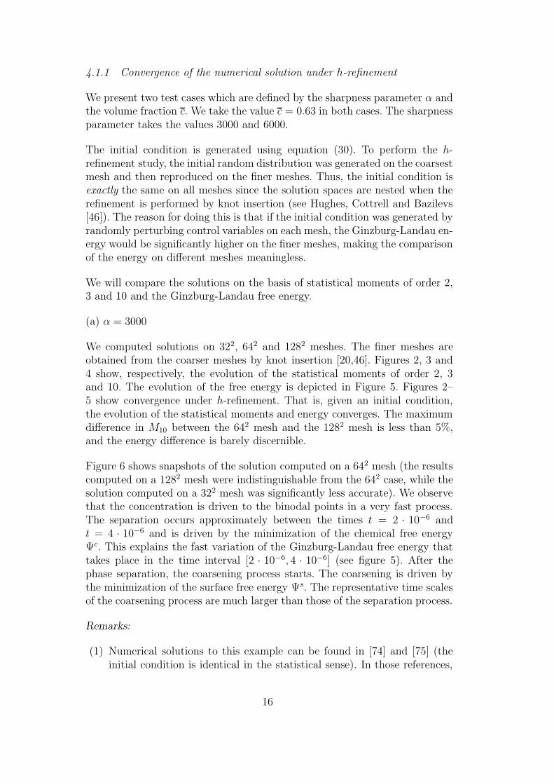
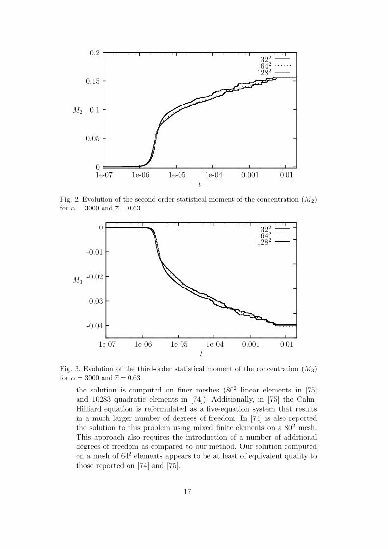
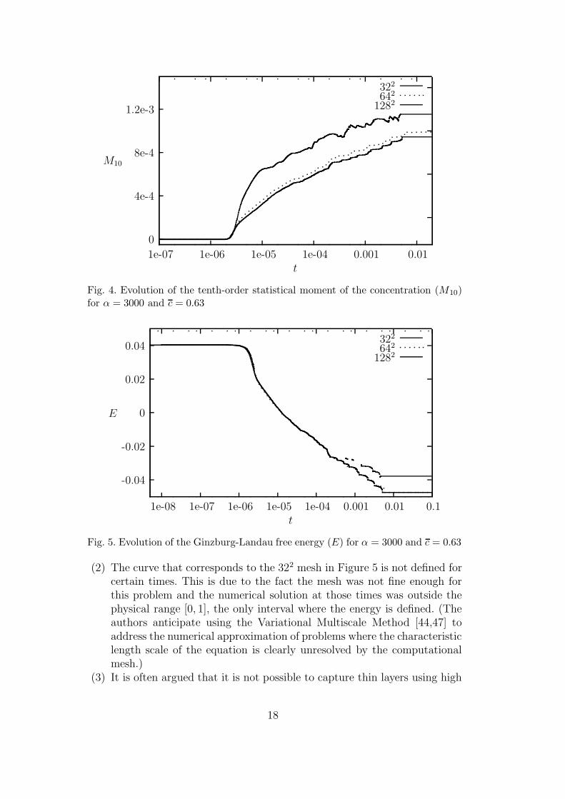
We computed solutions on 322, 642 and 1282 meshes. The finer meshes areobtained from the coarser meshes by knot insertion [20,46]. Figures 2, 3 and4 show, respectively, the evolution of the statistical moments of order 2, 3and 10. The evolution of the free energy is depicted in Figure 5. Figures 2–5 show convergence under h-refinement. That is, given an initial condition,the evolution of the statistical moments and energy converges. The maximumdifference in M10 between the 642 mesh and the 1282 mesh is less than 5%,and the energy difference is barely discernible.
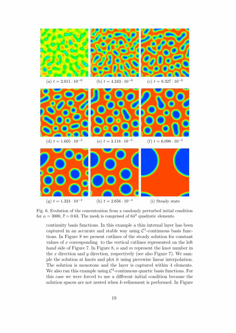
Figure 6 shows snapshots of the solution computed on a 642 mesh (the resultscomputed on a 1282 mesh were indistinguishable from the 642 case, while thesolution computed on a 322 mesh was significantly less accurate). We observethat the concentration is driven to the binodal points in a very fast process.The separation occurs approximately between the times t = 2 · 10−6 andt = 4 · 10−6 and is driven by the minimization of the chemical free energyΨc. This explains the fast variation of the Ginzburg-Landau free energy thattakes place in the time interval [2 · 10−6, 4 · 10−6] (see figure 5). After thephase separation, the coarsening process starts. The coarsening is driven bythe minimization of the surface free energy Ψs. The representative time scalesof the coarsening process are much larger than those of the separation process.
Remarks:
(1) Numerical solutions to this example can be found in [74] and [75] (theinitial condition is identical in the statistical sense). In those references,
16
0
0.05
0.1
0.15
0.2
1e-07 1e-06 1e-05 1e-04 0.001 0.01
M2
t
322
642
1282
Fig. 2. Evolution of the second-order statistical moment of the concentration (M2)for α = 3000 and c = 0.63
-0.04
-0.03
-0.02
-0.01
0
1e-07 1e-06 1e-05 1e-04 0.001 0.01
M3
t
322
642
1282
Fig. 3. Evolution of the third-order statistical moment of the concentration (M3)for α = 3000 and c = 0.63
the solution is computed on finer meshes (802 linear elements in [75]and 10283 quadratic elements in [74]). Additionally, in [75] the Cahn-Hilliard equation is reformulated as a five-equation system that resultsin a much larger number of degrees of freedom. In [74] is also reportedthe solution to this problem using mixed finite elements on a 802 mesh.This approach also requires the introduction of a number of additionaldegrees of freedom as compared to our method. Our solution computedon a mesh of 642 elements appears to be at least of equivalent quality tothose reported on [74] and [75].
17
0
4e-4
8e-4
1.2e-3
1e-07 1e-06 1e-05 1e-04 0.001 0.01
M10
t
322
642
1282
Fig. 4. Evolution of the tenth-order statistical moment of the concentration (M10)for α = 3000 and c = 0.63
-0.04
-0.02
0
0.02
0.04
1e-08 1e-07 1e-06 1e-05 1e-04 0.001 0.01 0.1
E
t
322
642
1282
Fig. 5. Evolution of the Ginzburg-Landau free energy (E) for α = 3000 and c = 0.63
(2) The curve that corresponds to the 322 mesh in Figure 5 is not defined forcertain times. This is due to the fact the mesh was not fine enough forthis problem and the numerical solution at those times was outside thephysical range [0, 1], the only interval where the energy is defined. (Theauthors anticipate using the Variational Multiscale Method [44,47] toaddress the numerical approximation of problems where the characteristiclength scale of the equation is clearly unresolved by the computationalmesh.)
(3) It is often argued that it is not possible to capture thin layers using high
18
(a) t = 2.011 · 10−6 (b) t = 4.243 · 10−6 (c) t = 8.327 · 10−6
(d) t = 1.605 · 10−5 (e) t = 3.118 · 10−5 (f) t = 6.098 · 10−5
(g) t = 1.324 · 10−4 (h) t = 2.656 · 10−4 (i) Steady state
Fig. 6. Evolution of the concentration from a randomly perturbed initial conditionfor α = 3000, c = 0.63. The mesh is comprised of 642 quadratic elements.
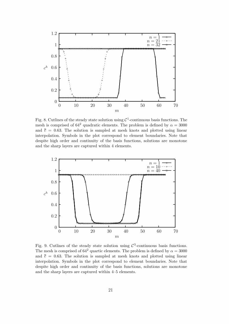
continuity basis functions. In this example a thin internal layer has beencaptured in an accurate and stable way using C1-continuous basis func-tions. In Figure 8 we present cutlines of the steady solution for constantvalues of x corresponding to the vertical cutlines represented on the lefthand side of Figure 7. In Figure 8, n and m represent the knot number inthe x direction and y direction, respectively (see also Figure 7). We sam-ple the solution at knots and plot it using piecewise linear interpolation.The solution is monotone and the layer is captured within 4 elements.We also ran this example using C3-continuous quartic basis functions. Forthis case we were forced to use a different initial condition because thesolution spaces are not nested when k-refinement is performed. In Figure
19

Fig. 7. Steady state solutions of the problem defined by α = 3000 and c = 0.63.In both pictures (left and right), the initial condition is the same from a statisticalpoint of view, but not from a deterministic point of view. The mesh is comprised of642 quadratic C1-continuous elements for the solution on the left hand side and 642
quartic C3-continuous elements for the solution on the right hand side. The verticallines on the left and right hand side pictures represent the cutlines that have beenplotted in Figure 8 and 9, respectively.
9 we represent cutlines of the steady state solution for constant valuesof x (this corresponds to the vertical cutlines on the right hand side ofFigure 7).
(b) α = 6000
This test case is more challenging than the previous one, because the param-eter α is larger. This means that the interfaces are thinner, which, in turn,requires a finer spatial mesh. In addition, this case is more interesting fromthe physical point of view, since phase-field models tend to sharp-interfacemodels as the thickness of the interfaces tends to zero.
We computed solutions on 642, 1282 and 2562 meshes. We plot snapshots ofthe solution computed on the 642 and 1282 meshes. The results on the 2562
mesh were indistinguishable from those on the 1282 mesh.
In Figures 10 and 11 we observe that the solutions at early and medium timeson the 642 and 1282 meshes are very similar. Only at the steady state do the so-lutions have significant differences. This example shows the difficulty involvedin computing steady-state solutions to the Cahn-Hilliard equation. Obtainingstationary solutions is much more challenging than computing transient solu-tions at early and medium times not only from the point of view of the timeintegration, but also from the point of view of the spatial discretization.
The modification of the parameter α has not only changed the thickness of
20
0
0.2
0.4
0.6
0.8
1
1.2
0 10 20 30 40 50 60 70
ch
m
n = 1
333333333333333333333333333333333333
3
3
3
3333333333333333333
3
3
3
3333
3
n = 21
+++
+
+
+
+
+
+
++++++++++++++
+
+
+
+
+
+
+
+++++++++++++++++++++++++++++++++++
+
n = 3222222222222222222222222222222222222222222222222222222222222222222
2
Fig. 8. Cutlines of the steady state solution using C1-continuous basis functions. Themesh is comprised of 642 quadratic elements. The problem is defined by α = 3000and c = 0.63. The solution is sampled at mesh knots and plotted using linearinterpolation. Symbols in the plot correspond to element boundaries. Note thatdespite high order and continuity of the basis functions, solutions are monotoneand the sharp layers are captured within 4 elements.
0
0.2
0.4
0.6
0.8
1
1.2
0 10 20 30 40 50 60 70
ch
m
n = 1
3333333333333333
3
3
3
3
3
33333333333333333
3
3
3
3
3
3333333333333333333333
3
n = 10
+++++++++++++++++++++++++++++++++++++++++++++++++++++++++++++++++
+
n = 4022222222
2
2
2
2222222222222222222222222222222222222
2
2
2
22222222222222
2
Fig. 9. Cutlines of the steady state solution using C3-continuous basis functions.The mesh is comprised of 642 quartic elements. The problem is defined by α = 3000and c = 0.63. The solution is sampled at mesh knots and plotted using linearinterpolation. Symbols in the plot correspond to element boundaries. Note thatdespite high order and continuity of the basis functions, solutions are monotoneand the sharp layers are captured within 4–5 elements.
21
(a) t = 1.878 · 10−6 (b) t = 4.060 · 10−6 (c) t = 8.042 · 10−6
(d) t = 1.598 · 10−5 (e) t = 3.270 · 10−5 (f) t = 6.274 · 10−5
(g) t = 1.257 · 10−4 (h) t = 2.665 · 10−4 (i) Steady state
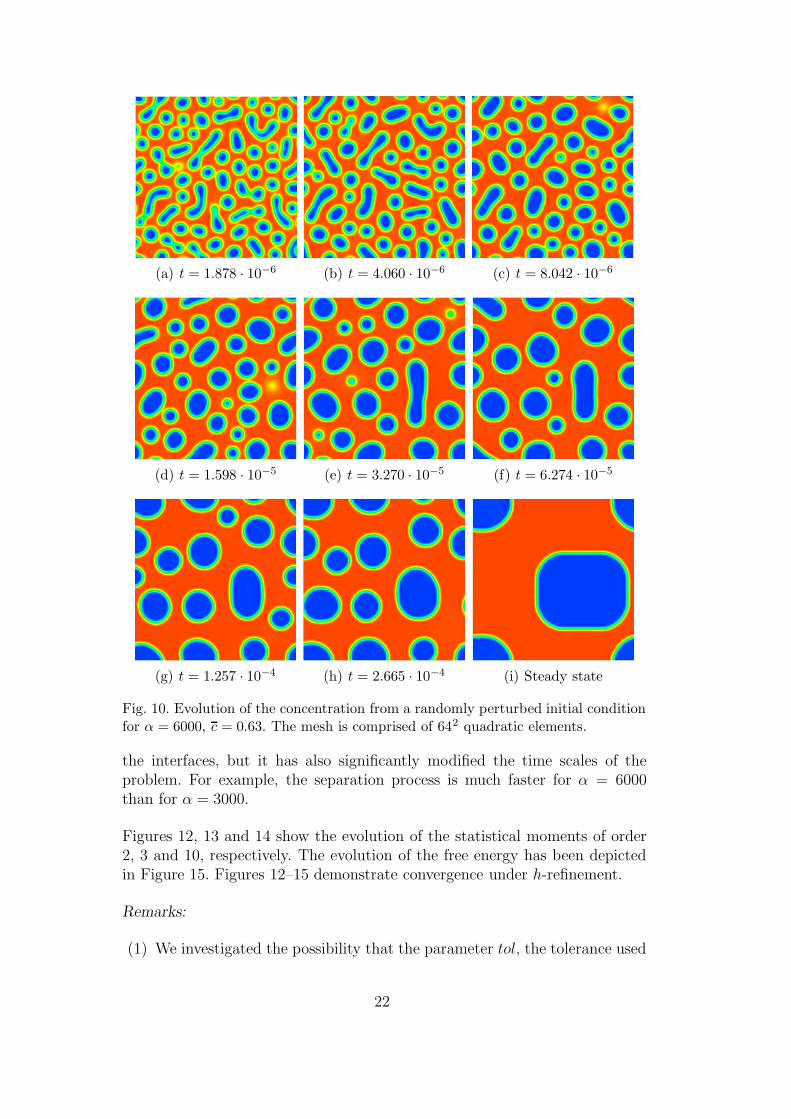
Fig. 10. Evolution of the concentration from a randomly perturbed initial conditionfor α = 6000, c = 0.63. The mesh is comprised of 642 quadratic elements.
the interfaces, but it has also significantly modified the time scales of theproblem. For example, the separation process is much faster for α = 6000than for α = 3000.
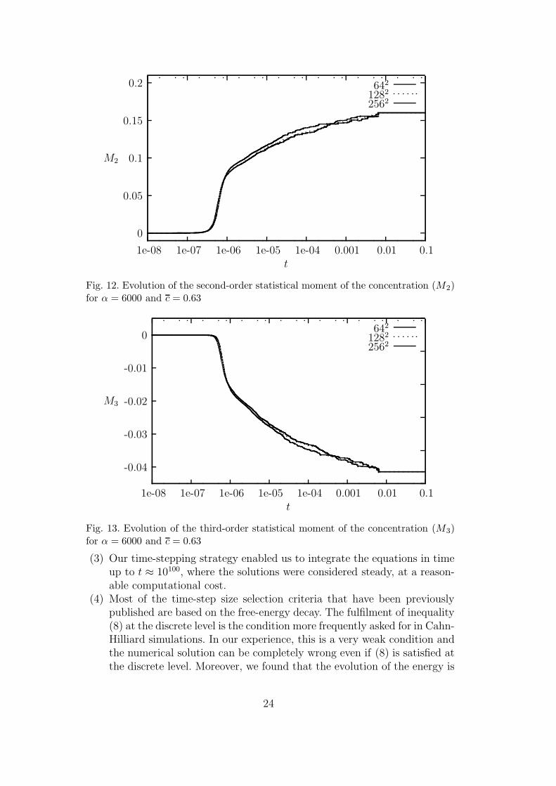
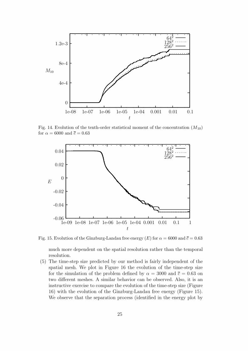
Figures 12, 13 and 14 show the evolution of the statistical moments of order2, 3 and 10, respectively. The evolution of the free energy has been depictedin Figure 15. Figures 12–15 demonstrate convergence under h-refinement.
Remarks:
(1) We investigated the possibility that the parameter tol, the tolerance used
22

(a) t = 1.837 · 10−6 (b) t = 3.821 · 10−6 (c) t = 7.801 · 10−6
(d) t = 1.641 · 10−5 (e) t = 3.246 · 10−5 (f) t = 6.190 · 10−5
(g) t = 1.237 · 10−4 (h) t = 2.557 · 10−4 (i) Steady state
Fig. 11. Evolution of the concentration from a randomly perturbed initial conditionfor α = 6000, c = 0.63. The mesh is comprised of 1282 quadratic elements.
to estimate the time-step size, affected the results. We ran cases withtol = 10−3 (our default value) and tol = 10−4. We found no discernibledifferences in the computed statistics, while the time-step size was signif-icantly smaller.
(2) We analyzed the performance of our time-step size predictor by runninga simple case taking a constant time-step size ∆t = 10−9 (this was lessthan the minimal time-step size employed by our time integrator for thatproblem). We found no discernible differences in the computed statistics,which suggests that our adaptive time-stepping technique gives us veryaccurate solutions at a small fraction of the cost of the constant time-stepstrategy.
23
0
0.05
0.1
0.15
0.2
1e-08 1e-07 1e-06 1e-05 1e-04 0.001 0.01 0.1
M2
t
642
1282
2562
Fig. 12. Evolution of the second-order statistical moment of the concentration (M2)for α = 6000 and c = 0.63
-0.04
-0.03
-0.02
-0.01
0
1e-08 1e-07 1e-06 1e-05 1e-04 0.001 0.01 0.1
M3
t
642
1282
2562
Fig. 13. Evolution of the third-order statistical moment of the concentration (M3)for α = 6000 and c = 0.63
(3) Our time-stepping strategy enabled us to integrate the equations in timeup to t ≈ 10100, where the solutions were considered steady, at a reason-able computational cost.
(4) Most of the time-step size selection criteria that have been previouslypublished are based on the free-energy decay. The fulfilment of inequality(8) at the discrete level is the condition more frequently asked for in Cahn-Hilliard simulations. In our experience, this is a very weak condition andthe numerical solution can be completely wrong even if (8) is satisfied atthe discrete level. Moreover, we found that the evolution of the energy is
24
0
4e-4
8e-4
1.2e-3
1e-08 1e-07 1e-06 1e-05 1e-04 0.001 0.01 0.1
M10
t
642
1282
2562
Fig. 14. Evolution of the tenth-order statistical moment of the concentration (M10)for α = 6000 and c = 0.63
-0.06
-0.04
-0.02
0
0.02
0.04
1e-09 1e-08 1e-07 1e-06 1e-05 1e-04 0.001 0.01 0.1 1
E
t
642
1282
2562
Fig. 15. Evolution of the Ginzburg-Landau free energy (E) for α = 6000 and c = 0.63
much more dependent on the spatial resolution rather than the temporalresolution.
(5) The time-step size predicted by our method is fairly independent of thespatial mesh. We plot in Figure 16 the evolution of the time-step sizefor the simulation of the problem defined by α = 3000 and c = 0.63 ontwo different meshes. A similar behavior can be observed. Also, it is aninstructive exercise to compare the evolution of the time-step size (Figure16) with the evolution of the Ginzburg-Landau free energy (Figure 15).We observe that the separation process (identified in the energy plot by
25
1e-08
1e-07
1e-06
1e-05
1e-04
0.001
0.01
1e-06 1e-05 1e-04 0.001 0.01
∆t
t
642
1282
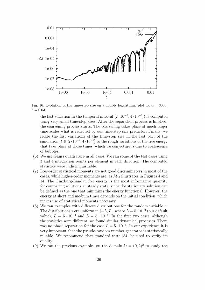
Fig. 16. Evolution of the time-step size on a doubly logarithmic plot for α = 3000,c = 0.63
the fast variation in the temporal interval [2 · 10−6, 4 · 10−6]) is computedusing very small time-step sizes. After the separation process is finished,the coarsening process starts. The coarsening takes place at much largertime scales what is reflected by our time-step size predictor. Finally, werelate the fast variations of the time-step size in the last part of thesimulation, t ∈ [2 ·10−4, 4 ·10−2] to the rough variations of the free energythat take place at those times, which we conjecture is due to coalescenceof bubbles.
(6) We use Gauss quadrature in all cases. We ran some of the test cases using3 and 4 integration points per element in each direction. The computedstatistics were indistinguishable.
(7) Low-order statistical moments are not good discriminators in most of thecases, while higher-order moments are, as M10 illustrates in Figures 4 and14. The Ginzburg-Landau free energy is the most informative quantityfor comparing solutions at steady state, since the stationary solution canbe defined as the one that minimizes the energy functional. However, theenergy at short and medium times depends on the initial condition, whichmakes use of statistical moments necessary.
(8) We ran examples with different distributions for the random variable r.The distributions were uniform in [−L, L], where L = 5·10−2 (our defaultvalue), L = 5 · 10−4 and L = 5 · 10−5. In the first two cases, althoughthe statistics were different, we found similar dynamical processes. Therewas no phase separation for the case L = 5 · 10−5. In our experience it isvery important that the pseudo-random number generator is statisticallyreliable. We recommend that standard tests [54] be used to verify itsquality.
(9) We ran the previous examples on the domain Ω = (0, 2)2 to study the
26
0
0.05
0.1
0.15
0.2
0.25
1e-08 1e-07 1e-06 1e-05 1e-04 0.001 0.01 0.1 1
M2, M4
t
M2M4
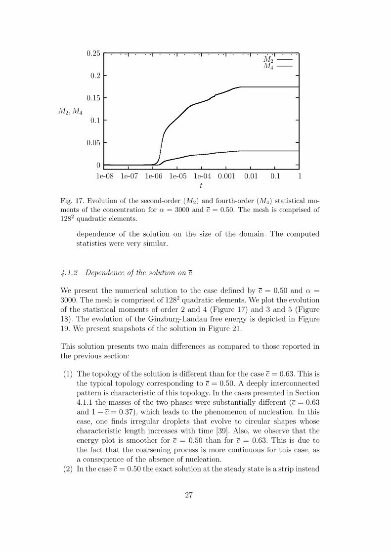
Fig. 17. Evolution of the second-order (M2) and fourth-order (M4) statistical mo-ments of the concentration for α = 3000 and c = 0.50. The mesh is comprised of1282 quadratic elements.
dependence of the solution on the size of the domain. The computedstatistics were very similar.
4.1.2 Dependence of the solution on c
We present the numerical solution to the case defined by c = 0.50 and α =3000. The mesh is comprised of 1282 quadratic elements. We plot the evolutionof the statistical moments of order 2 and 4 (Figure 17) and 3 and 5 (Figure18). The evolution of the Ginzburg-Landau free energy is depicted in Figure19. We present snapshots of the solution in Figure 21.
This solution presents two main differences as compared to those reported inthe previous section:
(1) The topology of the solution is different than for the case c = 0.63. This isthe typical topology corresponding to c = 0.50. A deeply interconnectedpattern is characteristic of this topology. In the cases presented in Section4.1.1 the masses of the two phases were substantially different (c = 0.63and 1− c = 0.37), which leads to the phenomenon of nucleation. In thiscase, one finds irregular droplets that evolve to circular shapes whosecharacteristic length increases with time [39]. Also, we observe that theenergy plot is smoother for c = 0.50 than for c = 0.63. This is due tothe fact that the coarsening process is more continuous for this case, asa consequence of the absence of nucleation.
(2) In the case c = 0.50 the exact solution at the steady state is a strip instead
27
0
4e-4
8e-4
1.2e-3
1e-08 1e-07 1e-06 1e-05 1e-04 0.001 0.01 0.1 1
M3, M5
t
M3M5
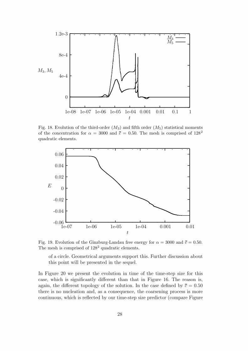
Fig. 18. Evolution of the third-order (M3) and fifth order (M5) statistical momentsof the concentration for α = 3000 and c = 0.50. The mesh is comprised of 1282
quadratic elements.
-0.06
-0.04
-0.02
0
0.02
0.04
0.06
1e-07 1e-06 1e-05 1e-04 0.001 0.01
E
t
Fig. 19. Evolution of the Ginzburg-Landau free energy for α = 3000 and c = 0.50.The mesh is comprised of 1282 quadratic elements.
of a circle. Geometrical arguments support this. Further discussion aboutthis point will be presented in the sequel.
In Figure 20 we present the evolution in time of the time-step size for thiscase, which is significantly different than that in Figure 16. The reason is,again, the different topology of the solution. In the case defined by c = 0.50there is no nucleation and, as a consequence, the coarsening process is morecontinuous, which is reflected by our time-step size predictor (compare Figure
28
1e-08
1e-07
1e-06
1e-05
1e-04
0.001
1e-07 1e-06 1e-05 1e-04 0.001 0.01
∆t
t
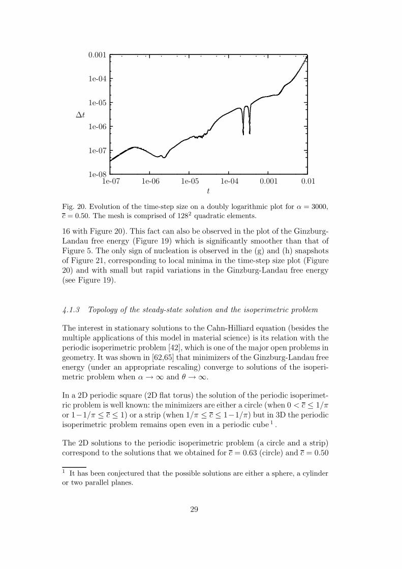
Fig. 20. Evolution of the time-step size on a doubly logarithmic plot for α = 3000,c = 0.50. The mesh is comprised of 1282 quadratic elements.
16 with Figure 20). This fact can also be observed in the plot of the Ginzburg-Landau free energy (Figure 19) which is significantly smoother than that ofFigure 5. The only sign of nucleation is observed in the (g) and (h) snapshotsof Figure 21, corresponding to local minima in the time-step size plot (Figure20) and with small but rapid variations in the Ginzburg-Landau free energy(see Figure 19).
4.1.3 Topology of the steady-state solution and the isoperimetric problem
The interest in stationary solutions to the Cahn-Hilliard equation (besides themultiple applications of this model in material science) is its relation with theperiodic isoperimetric problem [42], which is one of the major open problems ingeometry. It was shown in [62,65] that minimizers of the Ginzburg-Landau freeenergy (under an appropriate rescaling) converge to solutions of the isoperi-metric problem when α→∞ and θ →∞.
In a 2D periodic square (2D flat torus) the solution of the periodic isoperimet-ric problem is well known: the minimizers are either a circle (when 0 < c ≤ 1/πor 1−1/π ≤ c ≤ 1) or a strip (when 1/π ≤ c ≤ 1−1/π) but in 3D the periodicisoperimetric problem remains open even in a periodic cube 1 .
The 2D solutions to the periodic isoperimetric problem (a circle and a strip)correspond to the solutions that we obtained for c = 0.63 (circle) and c = 0.50
1 It has been conjectured that the possible solutions are either a sphere, a cylinderor two parallel planes.
29
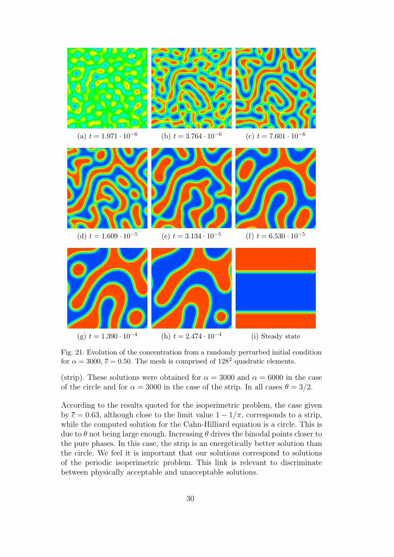
(a) t = 1.971 · 10−6 (b) t = 3.764 · 10−6 (c) t = 7.601 · 10−6
(d) t = 1.609 · 10−5 (e) t = 3.134 · 10−5 (f) t = 6.530 · 10−5
(g) t = 1.390 · 10−4 (h) t = 2.474 · 10−4 (i) Steady state
Fig. 21. Evolution of the concentration from a randomly perturbed initial conditionfor α = 3000, c = 0.50. The mesh is comprised of 1282 quadratic elements.
(strip). These solutions were obtained for α = 3000 and α = 6000 in the caseof the circle and for α = 3000 in the case of the strip. In all cases θ = 3/2.
According to the results quoted for the isoperimetric problem, the case givenby c = 0.63, although close to the limit value 1− 1/π, corresponds to a strip,while the computed solution for the Cahn-Hilliard equation is a circle. This isdue to θ not being large enough. Increasing θ drives the binodal points closer tothe pure phases. In this case, the strip is an energetically better solution thanthe circle. We feel it is important that our solutions correspond to solutionsof the periodic isoperimetric problem. This link is relevant to discriminatebetween physically acceptable and unacceptable solutions.
30
Remark:
If the Cahn-Hilliard phase-field model is to be used for the approximationof solutions of the isoperimetric problem, the authors recommend the useof constant mobility and quartic chemical potential, which also converges tosolutions of the isoperimetric problem as α→∞, but requires a significantlysmaller compute time.
4.1.4 Mesh-independent Cahn-Hilliard phase-field model
The Cahn-Hilliard phase-field model converges, in a thermodynamically con-sistent fashion, to its corresponding sharp-interface model as
√λ (the charac-
teristic length scale of the model) tends to zero. In order for the Cahn-Hilliardphase-field model to be realistic for engineering applications, λ has to be ex-tremely small. On the other hand, if the computational mesh is not fine enoughto resolve the internal layers whose size is defined by the length scale
√λ, non-
physical solutions are obtained.
To desensitize this mesh dependence, we propose to relate the characteristiclength scale of the continuous phase-field model to the characteristic lengthscale of the computational mesh. In the ideal case we would obtain the bestapproximation to the sharp-interface model for a given mesh. Also, we areseeking a method that preserves the topology of the solution at the steadystate independently of the mesh size while the thickness of the interface isenlarged according to the spatial resolution.
Numerical results using
λ = τh2, (32)
where τ is a dimensionless constant, have shown the potential of this approach.The value of τ has been determined by means of numerical examples. It turnedout that the maximum value of τ that can be used retaining mesh invariancedepends on the average concentration c. The closer c is to 0.5 the larger τ hasto be and, consequently, the thicker the interface. We show examples usingτ = 1 for c = 0.63 and τ = 2.5 for c = 0.50. The results are encouraging.
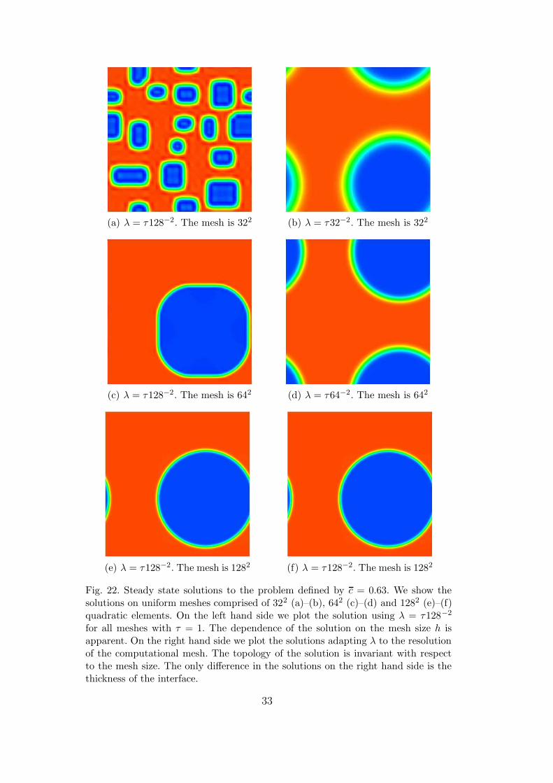
In the first example, c = 0.63. In Figure 22 we show the solutions on uni-form meshes comprised of 322, 642 and 1282 quadratic elements. The initialcondition is generated by randomly perturbing control variables on the 322
mesh and then it is exactly reproduced on the finer meshes as in the previousnumerical examples. On the left hand side, we plot the solution using for allmeshes λ = τ128−2 where τ = 1. We find a strong dependence of the solutionon the mesh size. On the right hand side we plot the solution adapting λ tothe resolution of the computational mesh through use of equation (32) withτ = 1. In this case, the topology of the numerical solution is independent of
31
the mesh size and the interface is captured on all meshes within 4–5 elements.
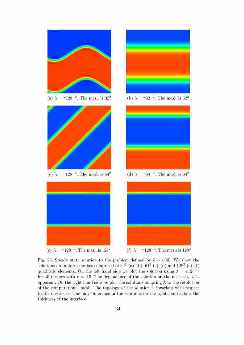
In the second example, c = 0.5. In Figure 23 we show the solution on uniformmeshes comprised of 322, 642 and 1282 quadratic elements. The initial condi-tion is generated in the same way as in the previous example. The solutions onthe left hand side have been computed using λ = τ128−2 for all meshes withτ = 2.5. A strong dependence of the solution on mesh size is observed. Thesolutions on the right hand side of Figure 23 have been computed adapting λto the resolution of the computational mesh using equation (32) and τ = 2.5.The topology of the numerical solution is again invariant with respect to themesh size and the interface is captured on all meshes within 4–5 elements.
The previous examples show the potential of the proposed approach to suc-cessfully deal with problems where the characteristic length scale of the contin-uous phase-field model is unresolved by the computational mesh. We believethat with this technique phase-field modeling, which has been used heretoforeprimarily in scientific studies, may become a practical engineering technology.
4.2 Numerical examples in three-dimensions
The complexity involved in the approximation of a 3D solution to the Cahn-Hilliard equation is much greater than for the 2D problem. The topology ofthe solution is much more complex and it experiences significant changes astime evolves. There seems to be almost nothing known about the steady statesolutions in 3D.
There are few references reporting numerical solutions to the Cahn-Hilliardphase-field model with degenerate mobility and logarithmic free energy. To ourknowledge, the numerical solutions presented in the literature are limited tothe early part of the simulation in 2D domains. We present herein stationarysolutions in 3D domains.
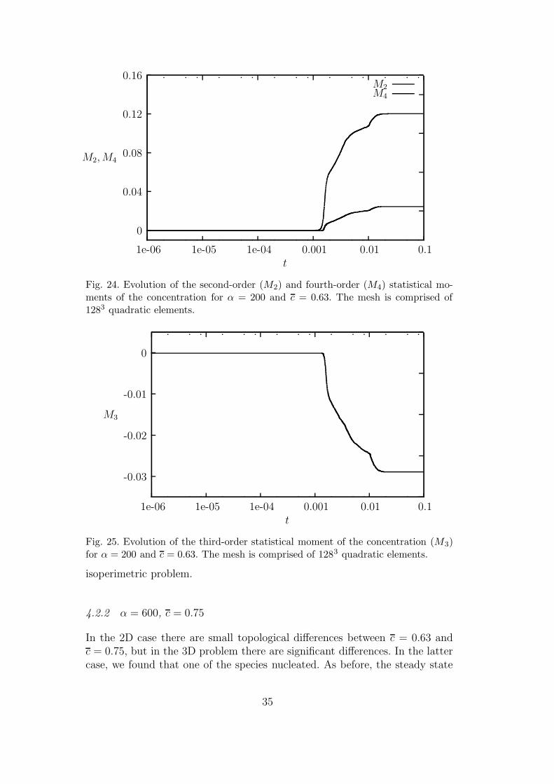
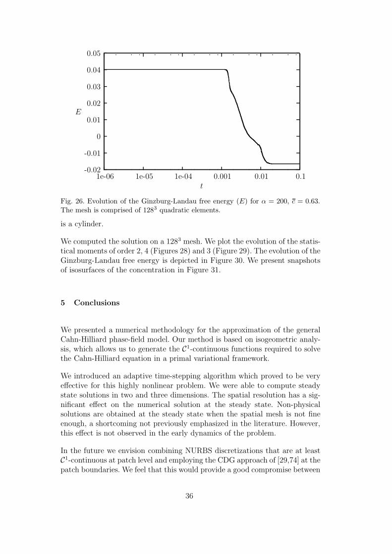
4.2.1 α = 200, c = 0.63
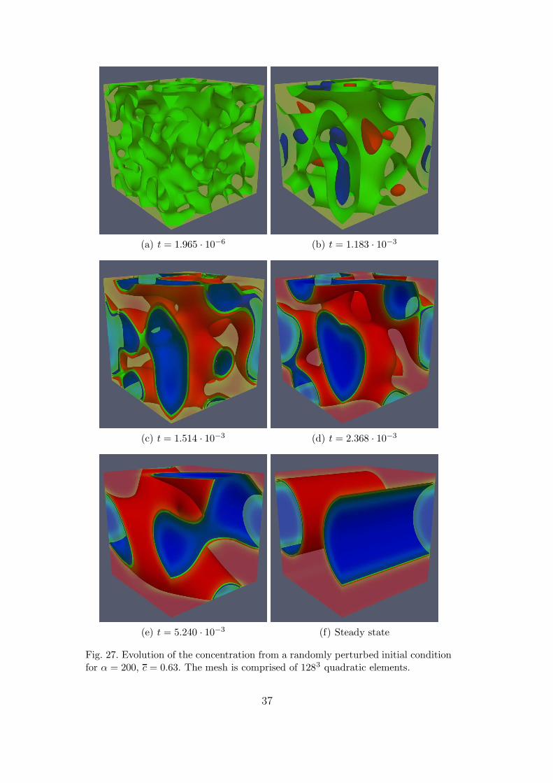
We computed the solution on a 1283 mesh. We plot the evolution of the statis-tical moments of order 2, 4 (Figure 24) and 3 (Figure 25). The evolution of theGinzburg-Landau free energy is depicted in Figure 26. We present snapshotsof isosurfaces of the concentration in Figure 27. We observe that the ran-domly perturbed constant concentration evolves to a complex interconnectedpattern. We did not find any sign of nucleation for this example, in contrastwith the 2D counterpart of this problem (see Section 4.1.1). The steady statesolution is a cylinder, which is one of the conjectured solutions for the periodic
32
(a) λ = τ128−2. The mesh is 322 (b) λ = τ32−2. The mesh is 322
(c) λ = τ128−2. The mesh is 642 (d) λ = τ64−2. The mesh is 642
(e) λ = τ128−2. The mesh is 1282 (f) λ = τ128−2. The mesh is 1282
Fig. 22. Steady state solutions to the problem defined by c = 0.63. We show thesolutions on uniform meshes comprised of 322 (a)–(b), 642 (c)–(d) and 1282 (e)–(f)quadratic elements. On the left hand side we plot the solution using λ = τ128−2
for all meshes with τ = 1. The dependence of the solution on the mesh size h isapparent. On the right hand side we plot the solutions adapting λ to the resolutionof the computational mesh. The topology of the solution is invariant with respectto the mesh size. The only difference in the solutions on the right hand side is thethickness of the interface.
33
(a) λ = τ128−2. The mesh is 322 (b) λ = τ32−2. The mesh is 322
(c) λ = τ128−2. The mesh is 642 (d) λ = τ64−2. The mesh is 642
(e) λ = τ128−2. The mesh is 1282 (f) λ = τ128−2. The mesh is 1282
Fig. 23. Steady state solution to the problem defined by c = 0.50. We show thesolutions on uniform meshes comprised of 322 (a)–(b), 642 (c)–(d) and 1282 (e)–(f)quadratic elements. On the left hand side we plot the solution using λ = τ128−2
for all meshes with τ = 2.5. The dependence of the solution on the mesh size h isapparent. On the right hand side we plot the solutions adapting λ to the resolutionof the computational mesh. The topology of the solution is invariant with respectto the mesh size. The only difference in the solutions on the right hand side is thethickness of the interface.
34
0
0.04
0.08
0.12
0.16
1e-06 1e-05 1e-04 0.001 0.01 0.1
M2, M4
t
M2M4
Fig. 24. Evolution of the second-order (M2) and fourth-order (M4) statistical mo-ments of the concentration for α = 200 and c = 0.63. The mesh is comprised of1283 quadratic elements.
-0.03
-0.02
-0.01
0
1e-06 1e-05 1e-04 0.001 0.01 0.1
M3
t
Fig. 25. Evolution of the third-order statistical moment of the concentration (M3)for α = 200 and c = 0.63. The mesh is comprised of 1283 quadratic elements.
isoperimetric problem.
4.2.2 α = 600, c = 0.75
In the 2D case there are small topological differences between c = 0.63 andc = 0.75, but in the 3D problem there are significant differences. In the lattercase, we found that one of the species nucleated. As before, the steady state
35
-0.02
-0.01
0
0.01
0.02
0.03
0.04
0.05
1e-06 1e-05 1e-04 0.001 0.01 0.1
E
t
Fig. 26. Evolution of the Ginzburg-Landau free energy (E) for α = 200, c = 0.63.The mesh is comprised of 1283 quadratic elements.
is a cylinder.
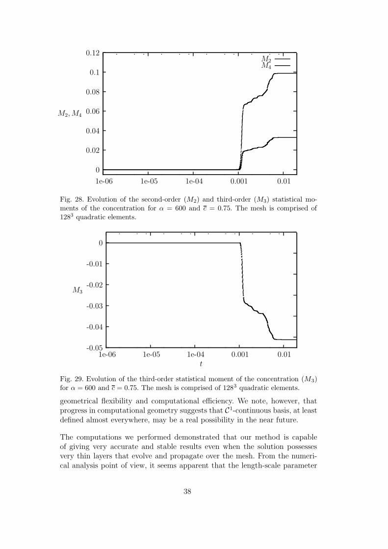
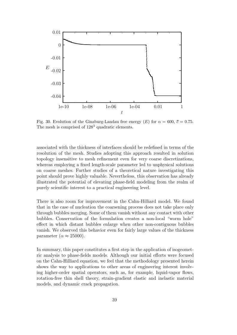
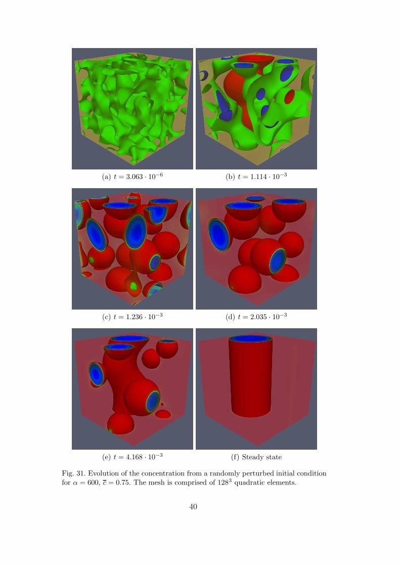
We computed the solution on a 1283 mesh. We plot the evolution of the statis-tical moments of order 2, 4 (Figures 28) and 3 (Figure 29). The evolution of theGinzburg-Landau free energy is depicted in Figure 30. We present snapshotsof isosurfaces of the concentration in Figure 31.
5 Conclusions
We presented a numerical methodology for the approximation of the generalCahn-Hilliard phase-field model. Our method is based on isogeometric analy-sis, which allows us to generate the C1-continuous functions required to solvethe Cahn-Hilliard equation in a primal variational framework.
We introduced an adaptive time-stepping algorithm which proved to be veryeffective for this highly nonlinear problem. We were able to compute steadystate solutions in two and three dimensions. The spatial resolution has a sig-nificant effect on the numerical solution at the steady state. Non-physicalsolutions are obtained at the steady state when the spatial mesh is not fineenough, a shortcoming not previously emphasized in the literature. However,this effect is not observed in the early dynamics of the problem.
In the future we envision combining NURBS discretizations that are at leastC1-continuous at patch level and employing the CDG approach of [29,74] at thepatch boundaries. We feel that this would provide a good compromise between
36
(a) t = 1.965 · 10−6 (b) t = 1.183 · 10−3
(c) t = 1.514 · 10−3 (d) t = 2.368 · 10−3
(e) t = 5.240 · 10−3 (f) Steady state
Fig. 27. Evolution of the concentration from a randomly perturbed initial conditionfor α = 200, c = 0.63. The mesh is comprised of 1283 quadratic elements.
37
0
0.02
0.04
0.06
0.08
0.1
0.12
1e-06 1e-05 1e-04 0.001 0.01
M2, M4
M2M4
Fig. 28. Evolution of the second-order (M2) and third-order (M3) statistical mo-ments of the concentration for α = 600 and c = 0.75. The mesh is comprised of1283 quadratic elements.
-0.05
-0.04
-0.03
-0.02
-0.01
0
1e-06 1e-05 1e-04 0.001 0.01
M3
t
Fig. 29. Evolution of the third-order statistical moment of the concentration (M3)for α = 600 and c = 0.75. The mesh is comprised of 1283 quadratic elements.
geometrical flexibility and computational efficiency. We note, however, thatprogress in computational geometry suggests that C1-continuous basis, at leastdefined almost everywhere, may be a real possibility in the near future.
The computations we performed demonstrated that our method is capableof giving very accurate and stable results even when the solution possessesvery thin layers that evolve and propagate over the mesh. From the numeri-cal analysis point of view, it seems apparent that the length-scale parameter
38
-0.04
-0.03
-0.02
-0.01
0
0.01
1e-10 1e-08 1e-06 1e-04 0.01 1
E
t
Fig. 30. Evolution of the Ginzburg-Landau free energy (E) for α = 600, c = 0.75.The mesh is comprised of 1283 quadratic elements.
associated with the thickness of interfaces should be redefined in terms of theresolution of the mesh. Studies adopting this approach resulted in solutiontopology insensitive to mesh refinement even for very coarse discretizations,whereas employing a fixed length-scale parameter led to unphysical solutionson coarse meshes. Further studies of a theoretical nature investigating thispoint should prove highly valuable. Nevertheless, this observation has alreadyillustrated the potential of elevating phase-field modeling from the realm ofpurely scientific interest to a practical engineering level.
There is also room for improvement in the Cahn-Hilliard model. We foundthat in the case of nucleation the coarsening process does not take place onlythrough bubbles merging. Some of them vanish without any contact with otherbubbles. Conservation of the formulation creates a non-local “worm hole”effect in which distant bubbles enlarge when other non-contiguous bubblesvanish. We observed this behavior even for fairly large values of the thicknessparameter (α ≈ 25000).
In summary, this paper constitutes a first step in the application of isogeomet-ric analysis to phase-fields models. Although our initial efforts were focusedon the Cahn-Hilliard equation, we feel that the methodology presented hereinshows the way to applications to other areas of engineering interest involv-ing higher-order spatial operators, such as, for example, liquid-vapor flows,rotation-free thin shell theory, strain-gradient elastic and inelastic materialmodels, and dynamic crack propagation.
39
(a) t = 3.063 · 10−6 (b) t = 1.114 · 10−3
(c) t = 1.236 · 10−3 (d) t = 2.035 · 10−3
(e) t = 4.168 · 10−3 (f) Steady state
Fig. 31. Evolution of the concentration from a randomly perturbed initial conditionfor α = 600, c = 0.75. The mesh is comprised of 1283 quadratic elements.
40
6 Acknowledgements
H. Gomez gratefully acknowledges the support provided by Ministerio de
Educacion y Ciencia through the postdoctoral fellowships program. Fund-ing provided by Xunta de Galicia (grants # PGIDIT05PXIC118002PN and# PGDIT06TAM11801PR), Ministerio de Educacion y Ciencia (grants #DPI2004-05156, # DPI2006-15275 and # DPI2007-61214) cofinanced withFEDER funds, Universidad de A Coruna and Fundacion de la Ingenierıa Civil
de Galicia is also acknowledged by H. Gomez. Y. Bazilevs was partially sup-ported by the J.T. Oden ICES Postdoctoral Fellowship at the Institute forComputational Engineering and Sciences. V.M. Calo, Y. Bazilevs and T.J.RHughes were partially supported by the Office of Naval Research under Con-tract No. N00014-03-0263 and under the MURI program (18412450-35520-B).
References
[1] H. Abels, M. Wilke, Convergence to equilibrium for the Cahn-Hilliardequation with a logarithmic free energy, Nonlinear Analysis: Theory Methods
& Applications 67 (2007) 3176–3193.
[2] D.M. Anderson, G.B. McFadden, A.A. Wheeler, Diffuse-interface methods influid mechanics, Annu. Rev. Fluid Mech. 30 (1998) 139–165.
[3] I. Akkerman, Y. Bazilevs, V. M. Calo, T. J. R. Hughes, S. Hulshoff, The roleof continuity in residual-based variational multiscale modeling of turbulence,Computational Mechanics 41 (2007) 371–378.
[4] J.W. Barret, J.F. Blowey, H. Garcke, Finite element approximation of the Cahn-Hilliard equation with degenerate mobility, SIAM Journal of Numerical Analysis
37 (1999) 286–318.
[5] J.W. Barrett, H. Garcke, R. Nurnberg, Finite element approximation of a phasefield model for surface diffusion of voids in a stressed solid, Mathematics of
Computation 75 (2006) 7–41.
[6] G.K. Batchelor, An introduction to fluid dynamics, Cambridge University Press,1967.
[7] Y. Bazilevs, V.M. Calo, J.A. Cottrell, T.J.R. Hughes, A. Reali, G. Scovazzi,Variational multiscale residual-based turbulence modeling for large eddysimulation of incompressible flows, Computer Methods in Applied Mechanics and
Engineering 197 (2007) 173–201.
[8] G. Benderskaya, M. Clemens, H. De Gersem, T. Weiland, Embedded Runge-Kutta methods for field-circuit coupled problems with switching elements, IEEE
Transactions on Magnetics 41 (2005) 1612–1615.
41
[9] J.F. Blowey, C.M. Elliott, The Cahn-Hilliard gradient theory for phase separationwith non-smooth free energy. Part II: Numerical analysis, European Journal of
Applied Mathematics 3 (1992) 147–149.
[10] G. Caginalp, Stefan and Hele-Shaw type models as asymptotic limits of thephase field equations, Phys. Rev. A 39 (1989) 5887–5896.
[11] J.W. Cahn, On spinodal decomposition, Acta Met. 9 (1961) 795–801.
[12] J.W. Cahn, J.E. Hilliard, Free energy of a non-uniform system. I. Interfacialfree energy, The Journal of Chemical Physics 28 (1958) 258–267.
[13] J.W. Cahn, J.E. Hilliard, Free energy of a non-uniform system. III. Nucleationin a two-component incompressible fluid, The Journal of Chemical Physics 31
(1959) 688–699.
[14] H.D. Ceniceros, A.M. Roma, A nonstiff adaptive mesh refinement-based methodfor the Cahn-Hilliard equation, Journal of Computational Physics 225 (2007)1849–1862.
[15] R. Chella, J. Vinals. Mixing of a two-phase fluid by cavity flow, Physical Review
E 53 (1996) 3832–3840.
[16] L.Q. Chen, Phase-field models for microstructural evolution, Ann. Rev. Mater.
Res. 32 (2002) 113–140.
[17] R. Choksi, P. Sternberg, Periodic phase separation: the periodic Cahn-Hilliardand the isoperimetric problems, Interfaces and Free Boundaries 8 (2006) 371–392.
[18] J. Chung, G.M. Hulbert, A time integration algorithm for structural dynamicswith improved numerical dissipation: The generalized-α method, Journal of
Applied Mechanics 60 (1993) 371–375.
[19] M.I.M. Copetti, C.M. Elliott, Numerical analysis of the Cahn-Hilliard equationwith a logarithmic free energy, Numerische Mathematik 63 (1992) 39–65.
[20] J.A. Cottrell, T.J.R. Hughes, A. Reali, Studies of refinement and continuity inisogeometric structural analysis, Computer Methods in Applied Mechanics and
Engineering 196 (2007) 4160–4183.
[21] J. Crank, Free and moving boundary problems, Oxford Univerrsity Press, 1997.
[22] A. Debussche, L. Dettori, On the Cahn-Hilliard equation with a logarithmicfree energy, Nonlinear Analysis 24 (1995) 1491–1514.
[23] I.C. Dolcetta, S.F. Vita, R. March, Area preserving curve-shortening flows:From phase separation to image processing, Interfaces and Free Boundaries 4
(2002) 325–343.
[24] Q. Du, R.A. Nicolaides, Numerical analysis of a continuum model of phasetransition, SIAM Journal of Numerical Analysis 28 (1991) 1310–1322.
42
[25] C.M. Elliott, D.A. French, Numerical studies of the Cahn-Hilliard equation forphase separation, IMA J. Appl. Math. 38 (1987) 97–128.
[26] C.M. Elliott, D.A. French, F.A. Milner, A 2nd-order splitting method for theCahn-Hilliard equation, Numerische Mathematiek 54 (1989) 575–590.
[27] C.M. Elliott, H. Garcke, On the Cahn-Hilliard equation with degeneratemobility, SIAM J. Math. Anal. 27 (1996) 404–423.
[28] C.M. Elliott, S. Zheng, On the Cahn-Hilliard equation, Archive for Rational
Mechanics and Analysis 96 (1986) 339–357.
[29] G. Engel, K. Garikipati, T.J.R. Hughes, M.G. Larson, L. Mazzei, R.L. Taylor,Continuous/discontinuous finite element approximations of fourth-order ellipticproblems in structural and continuum mechanics with applications to thinbeams and plates, and strain gradient elasticity, Computer Methods in Applied
Mechanics and Engineering 191 (2002) 3669–3750.
[30] D.N. Fan, L.Q. Chen, Diffuse interface description of grain boundary motion,Philosophical Magazine Letters 75 (1997) 187–196.
[31] X. Feng, A. Prohl, Analysis of a fully discrete finite element method for phasefield model and approximation of its sharp interface limits, Mathematics of
Computation 73 (2003) 541–547.
[32] I. Fonseca, M. Morini, Surfactants in foam stability: A phase field model, Arch.Ration. Mech. 183 (2007) 411-456
[33] H.B. Frieboes, J.P. Sinek, S. Sanga, F. Gentile, A. Granaldi, P. Decuzzi, C.Cosentino, F. Amato, M. Ferrari, V. Cristini, Towards Multiscale Modeling ofNanovectored Delivery of Therapeutics to Cancerous Lesions, to appear
[34] E. Fried, M.E. Gurtin, Dynamic solid-solid transitions with phase characterizedby an order parameter, Phys. D, 72 (1994) 287–308.
[35] D. Furihata, A stable and conservative finite difference scheme for the Cahn-Hilliard equation, Numer. Math. 87 (2001) 675–699.
[36] H. Garcke, B. Nestler, A mathematical model for grain growth in thin metallicfilms, Math. Models Methods Appl. Sci. 10 (2000) 895–921.
[37] H. Garcke, B. Nestler, B. Stinner, A diffuse interface model for alloys withmultiple components and phases, SIAM Journal of Applied Mathematics, 64
(2004) 775–799.
[38] H. Garcke, B. Nestler, B. Stoth, On anisotropic order parameter models formultiphase systems and their sharp interface limits, Phys. D 115 (1998) 87–108.
[39] H. Garcke, B. Niethammer, M. Rumpf, U. Weikard, Transient coarseningbehaviour in the Cahn-Hilliard model, Acta Materialia 51 (2003) 2823–2830.
[40] H. Garcke, A. Novick-Cohen, A singular limit for a system of degenerate Cahn-Hilliard equations, Adv. Differential equations 5 (2000) 401–434.
43
[41] K. Gustafsson, Control-theoretic techniques for stepsize selection in implicitRunge-Kutta methods, ACM Transactions on Mathematical Software 20 (1994)496–517.
[42] L. Hauswirth, J. Perez, P. Romon, A. Ros, The periodic isoperimetric problem,Transactions of the AMS 356 (2004) 2025–2047.
[43] Y. He, Y. Liu, T. Tang, On large time-stepping methods for the Cahn-Hilliardequation, Applied Numerical Mathematics, 57 (2007) 616–628.
[44] T.J.R. Hughes, Multiscale phenomena: Green’s functions, the Dirichlet-to-Neumann formulation, subgrid-scale models, bubbles and the origin of stabilizedmethods, Computer Methods in Applied Mechanics and Engineering, 127 (1995)387-401.
[45] T.J.R. Hughes, The Finite Element Method: Linear Static and Dynamic Finite
Element Analysis, Dover Publications, Mineola, NY, 2000.
[46] T.J.R. Hughes, J.A. Cottrell, Y. Bazilevs, Isogeometric analysis: CAD, finiteelements, NURBS, exact geometry and mesh refinement, Computer Methods in
Applied Mechanics and Engineering, 194 (2005) 4135–4195.
[47] T.J.R. Hughes, G.R. Feijoo, L. Mazzei, J.-B. Quincy, The Variational MultiscaleMethod — a paradigm for computational mechanics, Computer Methods in
Applied Mechanics and Engineering, 166 (1998) 3–24.
[48] K.E. Jansen, C.H. Whiting, G.M. Hulbert, A generalized-α method forintegrating the filtered Navier-Stokes equations with a stabilized finite elementmethod, Computer Methods in Applied Mechanics and Engineering, 190 (1999)305–319.
[49] J.-H. Jeong, N. Goldenfeld, J. A. Dantzig, Phase field model for three-dimensional dendritic growth with fluid flow, Physical Review E 64 (2001) 1–14
[50] Y. Jingxue, L. Changchun, Regularity of solutions of the Cahn-Hilliard equationwith concentration dependent mobility, Nonlinear Analysis 45 (2001) 543–554.
[51] D. Kay, R. Welford, A multigrid finite element solver for the Cahn-Hilliardequation, Journal of Computaional Physics 212 (2006) 288–304.
[52] J. Kim, K. Kang, J. Lowengrub, Conservative multigrid methods for Cahn-Hilliard fluids, Journal of Computaional Physics 193 (2004) 511–543.
[53] Y-T. Kim, N. Provatas, N. Goldenfeld, J. A. Dantzig, Universal Dynamics ofPhase Field Models for Dendritic Growth, Physical Review E 59 (1999) 2546–2549
[54] D.E. Knuth, The art of computing programming. Vol 2, Addison-Wesley, 1997.
[55] D.J. Korteweg, Sur la forme que prenent les equations du mouvements desfluides si l’on tient compte des forces capilaires causees par des variations dedensite considerables mains continues et sur la theorie de la capillarite dansl’hypothese d’une varation continue de la densite, Arch. Neerl Sci. Exactes Nat.Ser. II 6 (1901), pp. 124.
44
[56] L.D. Landau, V.I. Ginzburg, On the theory of superconductivity, in Collected
papers of L.D. Landau, D. ter Haar, ed., Pergamon Oxford (1965) 626–633.
[57] J. Lang, Two-dimensional fully adaptive solutions of reaction-diffusionequations, Appl. Numer. Math. 18 (1995) 223–240
[58] H.-G. Lee, J. S. Lowengrub, J. Goodman, Modeling pinchoff and reconnectionin a Hele-Shaw cell. II. Analysis and simulation in the nonlinear regime, Physics
of Fluids 14 (2002) 514-545.
[59] J. Lighthill, Waves in fluids, Cambridge University Press, 1978.
[60] C. Liu, J. Shen, A phase field model for the mixture of two incompressible fluidsand its approximation by a Fourier-spectral method, Physica D, 179 (2003) 211–228.
[61] J. Lowengrub, L. Truskinovsky, Quasi-incompressible Cahn-Hilliard fluids andtopological transitions, Proc. Roy. Soc. London Ser. A 454 (1998) 2617–2654.
[62] L. Modica, The gradient theory of phase transitions and the minimal interfacecriterion, Arch. Ration. Mech. Anal. 98 (1987) 123–142.
[63] O. Penrose, P.C. Fife, Thermodynamically consistent models of phase field typefor the kinetics of phase transition, Phys. D 43 (1990) 44–62.
[64] Y. Saad, M.H. Schultz, GMRES: A generalized minimal residual algorithm forsolving nonsymmetric linear systems, SIAM Journal of Scientific and Statistical
Computing 7 (1986) 856–869.
[65] P. Sternberg, The effect of singular perturbation on nonconvex variationalproblems, Arch. Ration. Mech. Anal. 101 (1988) 209–260.
[66] R.H. Stogner, G.F. Carey, C1 macroelements in adaptive finite elementmethods, International Journal for Numerical Methods in Engineering 70 (2007)1076-1095.
[67] Z.Z. Sun, A second order accurate linearized difference scheme for the two-dimensional Cahn-Hilliard equation, Mathematics of Computation 64 (1995)1463–1471.
[68] R. Toral, A. Chakrabarti, J.D. Gunton, Large scale simulations of the two-dimensional Cahn-Hilliard model, Physica A 213 (1995) 41–49.
[69] S. Tremaine, On the origin of irregular structure in Saturn’s rings, Astronomical
Journal 125 (2003) 894–901.
[70] H.S. Udaykumar, R. Mittal, W. Shyy, Computation of solid-liquid phase frontsin the sharp interface limit on fixed grids, Journal of Computational Physics 153
(1999) 535–574.
[71] P.J. van der Houwen, B.P. Sommeijer, W. Couzy, Embedded diagonally implicitRunge-Kutta algorithms on parallel computers, Mathematics of Computation 58
(1992) 135–159
45
[72] J.D. van der Waals, The thermodynamis theory of capillarity under thehypothesis of a continuous variation of density, J. Stat. Phys. 20 (1979) 197–244.
[73] B.P. Vollmayr-Lee, A.D. Rutemberg, Fast and accurate coarsening simulationwith an unconditionally stable time step, Physical Review E 68 (2003) 066703.
[74] G.N. Wells, E. Kuhl, K. Garikipati, A discontinuous Galerkin method for theCahn-Hilliard equation, Journal of Computaional Physics 218 (2006) 860–877.
[75] Y. Xia, Y. Xu, C.-W. Shu, Local discontinuous Galerkin methods for the Cahn-Hilliard type equations, Journal of Computational Physics 227 (2007) 472–491.
[76] X. Ye, X. Cheng, The Fourier spectral method for the Cahn-Hilliard equation,Applied Mathematics and Computation 171 (2005) 345–357.
[77] J. Zhu, L.-Q. Chen, J. Shen, V. Tikare, Coarsening kinetics from a variable-mobility Cahn-Hilliard equation: Application of a semi-implicit Fourier-spectralmethod, Physical Review E 60 3564–3572.
46
Related Documents


![Derivation of effective macroscopic Stokes–Cahn–Hilliard ...pavl/MSMPGPSKOct2013.pdf · assumption. In [24], it is shown that the Cahn–Hilliard or diffuse interface formulation](https://static.cupdf.com/doc/110x72/5f6cfdd72463bb71010538e3/derivation-of-effective-macroscopic-stokesacahnahilliard-pavlmsmpgpskoct2013pdf.jpg)