Investment and the Cost of Capital in the Nineties in ...

Investment and the Cost of Capital in the Nineties

in France: A Panel Data Investigation

by Jean-Bernard Chatelain and André Tiomo

in:

ifo StudienZeitschrift für empirische Wirtschaftsforschung

Jg. 48, Nr. 4, 2002, S. 655 –684

2002

ifo Studien ISSN 0018-9731Herausgeber: Prof. Dr. Gerhard IllingSchriftleitung: Dr. Marga Jennewein

Verlag:ifo Institut für WirtschaftsforschungPoschingerstr. 5, 81679 München

Tel. +49-89-9224-0 www.ifo.de

Kommerzielle Verwendung der Daten,auch über elektronische Medien,

nur mit Genehmigung des ifo Instituts.

brought to you by COREView metadata, citation and similar papers at core.ac.uk

provided by Research Papers in Economics

https://core.ac.uk/display/6939148?utm_source=pdf&utm_medium=banner&utm_campaign=pdf-decoration-v1

Investment and the Cost of Capital in the Ninetiesin France: A Panel Data Investigation∗∗∗∗

By Jean-Bernard Chatelain and André Tiomo

Contents

I. Introduction

II. The Intertemporal Behaviour of Firms

III. Data and Econometric Results

IV. Conclusion

I. Introduction

It is a widespread belief among economists that monetary policy affects the in-vestment of firms through the cost of capital and the credit channel. However, theavailable evidence shows that the cost of capital channel of monetary policy hasno effect on corporate investment in France at the macroeconomic level. ThreeFrench forecasting models developed in the 1990s do not include the cost ofcapital (see Amadeus by INSEE, Mosaïque by OFCE, and the model developedby the Banque de France), while INSEE's Metric model adds a relative factor costwhose parameter is small (-0.016) and not significant (see Assouline et al. 1998).Herbet (2001) published a recent estimation of macroeconomic investment andrecognised its failure to incorporate interest rate or user cost effects.

Four recent studies have focused on the effect of the user cost at the firmlevel. The results vary considerably. Using the BACH European database “aggre-gated by size and sector” based on Banque de France sample data, Beaudu andHeckel (2001) found a zero elasticity for the four largest euro area countries in-cluding France. Using the INSEE BIC-BRN database, Duhautois (2001) aggre-gated data by sector and size from 1985 to 1996. He found a real interest rateelasticity of -0.38 for the period 1985-1990 and of -0.27 for the period 1991-1996.Using a sample of individual firm accounts (INSEE BIC database), Crépon andGianella (2001) obtained a user cost elasticity of -0.63 for industry and of -0.35 forservices over the period 1990-1995. Using the BACH database, like Beaudu and

∗ We thank a referee for his very helpful comments as well as Steve Bond, Paul Butzen,

Marcel Gérard, Anil Kashyap and Philip Vermeulen and participants in the MonetaryTransmission Network of the Eurosystem of Central Banks, in the related European Cen-tral Bank conference and in the conference about “Corporate and Capital Income Taxationin the EU” in Mons University.

Jean-Bernhard Chatelain and André Tiomo

656

Heckel (2001), Mojon Smets and Vermeulen (2001) obtained a high elasticity forthe user cost for France (-0.75). These studies show that we obtain a high usercost elasticity if (1) the sample period is short and/or (2) the cash flow or thegrowth of sales is omitted from the regression and/or (3) within estimates areused instead of dynamic panel data estimates, as in the generalised method ofmoments (Arrelano and Bond (1991)) and/or (4) when defining the user cost, themarginal cost of debt is computed by a proxy at the firm level instead of an in-terest rate at the national level.

At the firm level, the existence of a broad credit channel of monetary policy inFrance is indirectly addressed. The main result is that financial variables (nota-bly cash flow) affect the investment of groups of firms that are likely to be finan-cially constrained (see Chatelain 2002). The interpretation of investment cashflow excess sensitivity for some group of firms as a signal of financial constraintshas been challenged by Kaplan and Zingales (1997). However, if the sampleseparation criterion is itself a precise measure of financial constraints, (e.g.credit rating is a more precise criterion to identify financially constrained firmsthan the low dividend payout criterion used by Fazzari, Hubbard and Petersen(1988)), the investment cash flow excess sensitivity is more likely to signal fi-nancial constraints than demand effects. Models which define investment as afunction of sales growth and cash flow have been around for a long time (seeBond et al. 1997; Hall, Mairesse, Mulkay 1999; 2000). Several recent studieshave estimated the excess sensitivity of investment to liquidity variables, suchas cash flow, the stock of cash, leverage and the coverage ratio. Crépon andRosenwald (2001) showed that the leverage parameter was lower for smallfirms during the years of sustained activity, i.e. 1988 and 1989 (their estimationperiod was 1986-1993). This means that the agency premium was lower forthese firms at that time. The neo-classical demand for capital estimated byBeaudu and Heckel (2001) led to greater investment cash flow sensitivity forsmall firms during years of monetary restriction. In Duhautois (2001), leverageexplains small firms’ investment from 1985 to 1996 in a regression where salesgrowth is an omitted variable. Using Euler investment equations, where the costof debt increases with leverage, Chatelain and Teurlai (2000) showed a cashflow misspecification (which is an indirect test of investment cash flow excesssensitivity consistent with the Lucas critique) for firms with a low dividend/payoutratio or a low investment/retained earnings ratio. Finally, Chatelain and Teurlai(2001) found that small firms with a high variation of debt and a high share ofcapital financed by leasing displayed an investment leverage excess sensitivityduring the economic downturn between 1993 and 1996.

This paper provides estimates of the elasticity of the user cost of capital andof investment cash flow excess sensitivities. We extend the analysis developedby Chatelain et al. (2001) by using more precise sample separation criteria toisolate financially constrained firms and by comparing several ways of testingauto-regressive distributed lags models of the neo-classical demand for capitalon a panel data of French manufacturing firms in the nineties (see Bond, Elston,Mairesse, Mulkay 1997 and Hall, Mairesse and Mulkay 2000; Harhoff and Ramb2001; Chirinko, Fazzari and Meyer 1999).

Section II presents the theoretical model of investment and the estimationmethod. Section III gives the macroeconomic background of investment and fi-

Investment and the Cost of Capital in the Nineties in France 657

657

nance of French companies in the nineties, describes the data set and empiricalresults. Section IV concludes.

II. The Intertemporal Behaviour of Firms

1. Theoretical Model

We consider a profit-maximising firm which does not face adjustment costs ofinvestment but does face tax deductibility of depreciation and interest chargesas well as a marginal cost of debt increasing with leverage. A one-period modelwas developed by Auerbach (1983) and Hayashi (2000) presented an intertem-poral continuous time version. Our presentation is based on discrete time in-tertemporal optimisation of firms facing uncertainty. With respect to King andFullerton's (1984) approach, we do not take into account the differences inhousehold taxation with respect to dividends and retained earnings nor the dis-tinction between different capital goods for the computation of the net presentvalue of depreciation allowances. We assume one financial constraint: the costof debt increases with leverage. However, a firm can always get round this con-straint using negative dividends or new share issues. We do not take into ac-count other financial constraints such as positive dividends, a transaction costfor new share issues, or a debt ceiling constraint.

Analysing investment begins with an expression of the value of the firm, whichin turn stems from the arbitrage condition governing the valuation of shares forrisk-neutral investors. The return for the risk-neutral owners of firm i at time treflects capital appreciation and current dividends. In equilibrium, if the ownersare to be content holding their shares, this return must equal tρ the nominalreturn on other risky financial assets between period t and period 1+t :1

(1) ( )[ ] ( )t

it

t,ititt,it,itV

dEVVEρ=

+−Ψ− +++ 111

In what follows, the subscript i always refers to firm i and the subscript t toyear t, tE is the expectation operator conditional on information known at timet , itd are dividends, itV is the firm's nominal market value (it is equal to the

number of existing shares times the share price Eitp ), itΨ is new share issues.

Solving this iterative arbitrage condition leads investors in firm i to choose thestock of capital and debt by maximizing the present value of dividends less newshare issues at time t in a infinite horizon:

(2){ }

[ ] max0

1

00ti,

0itit

t

t

sst

B,KdEV

itit

Ψ−

= ∑ ∏

∞

=

−

==∞

β ,

1 To be more precise, ρ is an expected return on a large number of risky financial assets

between date t and date 1+t . Applying the law of large numbers leads this expected returnto be considered as realized ex-post and therefore known with certainty ex-ante.


658

where the firm's one-period nominal discount factor is )/( tt ρβ += 11 . Investment

itI is defined by the capital stock itK accounting identity:

(3) ( ) 1 1−−−= t,iitit KKI δ ,

δ is the constant rate of economic depreciation. The flow of funds equation de-fines corporate dividends. Cash inflows include sales, new share issues, and netborrowing, while cash outflows consist of dividends, factor and interest pay-ments, and investment expenditures. Labour charges, interest charges and ac-counting depreciation are tax deductible. For simplification, we consider that ac-counting depreciation does not differ from economic depreciation. An investmenttax credit rate ititc is taken into account:

(4)( ) ( )[ ]

( ) ( )[ ] 1itc1

1

11

1111

−−

−−−−

−−−−−+Ψ+

+−−−=

t,iitIstitt,iitit

Sit

t,iIt,itt,it,iittititittit

KKpBBp

KpBiNwN,KFpd

δ

δττ

Where itN is a vector of variable factors of production, ( )itit N,KF is the firm'srevenue function ( 0 0 <> KKK F,F ), tw is a vector of nominal factor prices, iti isthe nominal interest rate on debt, itB is the value of net debt outstanding, itp is

the price of final goods, Istp is the sectoral price of capital goods; S

stp is theprice of new share issues; tτ is the corporate income tax rate, against whichinterest payments and depreciation are assumed to be deductible.

The nominal interest rate on debt at time t depends on an agency premiumwhich increases with debt and decreases with capital taken as collateral andtherefore valued by the current resale price of investment. We assume that thedebt interest rate increases with the debt/capital ratio: . 0 with, ) >'

ititIstitit iKp/B(i

After substitution of dividends by the flow of funds and of investment using thecapital stock equation, we provide first order conditions for the maximisation ofthe firm's value. First, the Euler equation with respect to debt is:

(5)

( )

( ) ( ) 01 1

0111

11

1

>

−=−−⇒

=

∂∂

+−+−

++

+

'it

itIst

itttitttt

itit

ititttit

iKp

BEiE

BBi

iE

ττρ

τβ

This condition shows that the optimal debt/capital ratio is independent fromthe choice of capital (the optimal debt/capital ratio is unique if for example

02 >+ ''' ii ). This optimal debt/capital ratio results from the trade-off between thetax advantage of debt and the increase of the agency costs premium. It is suchthat the optimal gap between the rate of return on equity (i.e. the opportunitycost of equity) and the net-of-tax marginal cost of debt is positive. The Eulerequation with respect to capital is:


659

(6)

( ) ( ) ( )

( )( ) ( )

( ) ( )( ) [ ].ccc

p

pCN,KF

iKp

BppE

pN,KFp

t

it

it

Ist

itititK

'it

itIst

itt

Istt

It,st,itt

IstitititKitt

321

2

2

1111

11

itc1

0 11itc1

itc11

−−−−

−==⇒

=

−++−−+

−−−

++++

τ

τδτδβ

τ

where the components of the cost of capital itC are:

( )( )

( )( ) I

stit

It,st,it

t p

pEc

itc1

itc1

11 11

1−

−

+−= ++

ρδ ,

( )[ ]( ) it

Istit

ititttt

Kp

BiEc

itc11 12

−−−= +τρ ,

( )it

ttEc

itc11

3 −= +τδ

.

Each of these three components depends on tax policy. The term 11 c− leadsto the Hall and Jorgenson (1967) formula for the cost of capital without tax dis-tortions between means of finance and between depreciated assets. Taxationmatters via the investment tax credit which decreases the price of investment.The term 2c is obtained after substitution using the Euler condition on debt. Itdecreases the cost of capital due to the tax deductibility of interest charges un-der the constraint of an increasing cost of debt as leverage increases. In this re-spect, a higher optimal leverage decreases the cost of capital. The term 3c de-creases the cost of capital due to the deductibility of depreciated capital. To takeinto account the case where accounting depreciation differs from constant eco-nomic depreciation, one has to cancel the third term of the cost of capital 3c

and substitute the correction of the investment price ( )ititc1− everywhere it ap-pears by ( )itit z−− itc1 , where itz is the net present value of depreciation allow-ances (Hayashi 2000, p.60).

Using a first order approximation with respect to the rate of depreciation, tothe tax-corrected inflation rate of the price of investment goods and to the rate ofreturn on equity, one finds a weighted average cost of capital used by appliedresearchers (the cost of equity and the after-tax cost of debt are weighted bytheir relative share with respect to capital).

(7)( )

( )( )

( )( ) ( )

( )

−

−−−−

−−+

−−+−

−=−−−

+++

+

Iitit

Iitit

It,it,it

it

tt

tit

Istit

itittt

itIstit

it

p

ppE

itcE

Kpitc

BiE

Kpitc

Bccc

itc1

itc1itc1

11

11 1

11

111

1321

δτ

ρτ


660

The Hayashi [2000, p.80] formula can be obtained by setting the investmenttax credit ititc to zero and by assuming a constant corporate income tax rate( 1+= t,itit E ττ ). In our applied work, we use:

(8) ( ) ( ) ( )

−−−+

++−

+−= +

It

It

It

stttitit

ititt

itit

it

tst

It

p

ppEB

EAI

EBB

pp

UC 1111

1 δτρττ

We set the investment tax credit rate to zero. The investment tax credit rate is0% for more than 80% of companies and over 95% for 5% of companies (hencecreating many outliers with near zero user cost), we finally did not take it intoaccount. We used an accounting measure of capital in leverage instead of aneconomic one: the denominator of leverage is the accounting sum of debt B andof equity E instead of the stock of capital computed by the perpetual inventorymethod. This is empirically justified on the grounds that it is the accounting pro-portions of debt or of equity which matter for tax deductibility. Using the stock ofcapital computed by the perpetual inventory method does not guarantee that theshare of debt in capital and the share of equity in capital sum to one. We use aproxy for the marginal cost of debt which has the drawback of being an averagerate itAI (the ratio of interest and similar charges to gross debt) but which as theadvantage of providing information at the firm level and of increasing the vari-ance of the user cost (61237 observations) with respect to a national annual ratethat we use for the opportunity cost of equity (10 observations, as the estimationperiod lasts 10 years).

With respect to the monetary transmission channels, this cost of capital takesinto account the interest rate channel, a part of the credit channel (leverage), theasset price channel (inflation rate of asset prices such as firms' property prices,and the price of collateralisable assets used in leverage), as well as potentialreactions to monetary policy of tax policies supporting corporate investment. Butit does not take into account other credit channel effects due to the existence ofa positive dividends constraint, whose Lagrange multiplier would alter the Eulerequation.

2. Parameterization and Econometric Model

We parameterize the production function as a constant elasticity of substitu-tion (CES) production function ( itS is sales):

(9) ( )υ

σσ

σσ

σσ

−−−

+==

111

itititititit bLaKAN,KFS

A, a, and b are productivity parameters, υ represents returns to scale and σ isthe elasticity of substitution between capital and labour. Computing the marginalproductivity of capital and taking logs (small letters represent logs of capital let-ters), we obtain this long-run demand for capital:


661

(10) ( ) ( )a.lnAlnc.sk itititit υσυ

σσυ

σσ +−−−

−+= 11

For simplification, productivity is assumed to be of the form 21 ηηtiit AAA = , so

that the constant and the productivity term ( ) ( )a.lnAln]/)[( it υσυσ +−− 1 are takeninto account by the constant related to individual firms (fixed effect) and the timedummies.

We assume an econometric adjustment process in the form of an auto-regressive distributed lag model with two lags with respect to the auto-regressive term and two lags with respect to explanatory variables (ADL(2,2)),as in Hall, Mairesse, Mulkay (2000). We consider four ways of estimating such amodel on panel data. The first one is exactly the ADL(2,2) specification:

(11)itti

t,iI

t,s

t,i

t,iI

t,s

t,i

t,iIst

it

t,it,iitt,it,iitt,it,iit

Kp

CF

Kp

CF

Kp

CF

cccssskkk

εααθθθ

σσσβββγγ

++++++

−−−++++=

−−

−

−−

−

−

−−−−−−

32

22

21

11

10

22110221102211

where iα is an individual constant (fixed effect), tα is a time constant (year ef-fect) and itε is a random shock. We add cash-flow (otherwise a potentiallyomitted variable, among other variables) on the grounds that our model does nottake fully into account financial constraints. The long-run elasticity of sales isgiven by )/()(LT 21210 1 γγββββ −−++= and the long-run elasticity of the costof capital is given by )/()(LT 21210 1 γγσσσσ −−++−=− . Return to scale is givenby )/()( LTLTLT σβσν −−= 1 . As explained later, we estimate this model in firstdifferences using the generalised method of moments (GMM). The endogenousvariable is then itk∆ where ∆ is the first difference operator ( 1−−=∆ t,iitit kkk ).

In model ADL-I, the aim is only to write the investment ratio as the explanatoryvariable. We subtract 1−t,ik from both sides in order to use the approximation

δ−=∆ − )K/I(k t,iitit 1 . The Taylor rest of the power series:

( )( ) ( )∑+∞

=− −−=

2111

j

jt,iit

jit ]K/I[j/R δ

is neglected. (We computed the stock of capital using the perpetual inventorymethod with a constant depreciation rate δ.)

(12)

( ) ( )

itti

t,iI

t,s

t,i

t,iI

t,s

t,i

t,iIst

itt,it,iit

t,it,iitt,it,i

t,i

t,iit

Kp

CF

Kp

CF

KpCFccc

ssskKI

KI

εαα

θθθσσσ

βββγγγ

+++

+++−−−

+++−++−=

−−

−

−−

−

−−−

−−−−

−

−

32

22

21

11

1022110

221102122

11

1

11


662

Estimated with GMM first differences, the endogenous variable is now the firstdifference of a growth rate. Due to the approximation, model ADL-I has thedrawback that the error term includes power series of the endogenous variableas the differences of the Taylor rest: 1−− t,iit RR . We intend to verify whether thisapproximation matters. Note that, as the value of current investment is deflatedby the price of current investment, we use the same deflator for cash flow.

The next model is the error correction model ECM(2,2) used on panel data byHall, Mairesse and Mulkay (2001) among others. They transform model ADL-Ias follows:

(13)

( ) ( ) ( )( )( )

ittit,i

It,s

t,i

t,iI

t,s

t,i

t,iIst

it

t,it,iitt,i

t,it,it,iitt,i

t,i

t,i

it

Kp

CF

Kp

CF

Kp

CF

cccs

skssKI

KI

εααθθθ

σσσγγβββ

γγβββγ

++++++

−−−−+++++

−−++∆++∆+−=

−−

−

−−

−

−

−−−

−−−−

−

−

32

22

21

11

10

22110212210

221211002

11

1

1

11

Error correction models have been introduced in time series analyses of co-integration. In particular, the long-run relationship is often estimated in a firststep, with residuals which are integrated of order zero, and the ECM is esti-mated for transitory dynamics as a second step. An argument is that theECM(2,2) on panel data can deal better with the unit root of the explained vari-able than the ADL(2,2) and ADL-I. First differences can remove the auto-correlation of one of the variables in the case of a unit root. A very high autocor-relation in panel data on firms is observed (Hall and Mairesse 2001). A draw-back of the ECM is that the test for necessary lags is not direct (in particular lag2) whereas they are directly obtained with the ADL specification. These tests areimportant because adding not significant lags can change dramatically the valueof long run elasticities, while these long run elasticities remain significant evenwith one or more not significant lags. One needs to recover parameters andstandard errors of the ADL(2,2) and ADL-I models from the ECM parametersand variance-covariance matrix. For this reason, it is more practical to estimatedirectly the ADL(2,2) and ADL-I models. We also estimate this ECM(2,2) modelto check its differences with the ADL(2,2) and ADL-I.

Using the same approximation as in model ADL-I so that the investment ratioappears as the explanatory variable instead of the log of capital, Chatelain et al.(2002), among others, used first differences of all the variables of the ADL(2,2)model and then added cash-flow. We label this the “difference ADL” model:

(14)

titi

t,iI

t,s

t,i

t,iI

t,s

t,i

t,iIst

itt,it,iit

t,it,iitt,i

t,i

t,i

t,i

t,iit

f

Kp

CF

Kp

CF

KpCFccc

sssKI

KI

KI

αε

θθθσσσ

βββγγ

+∆++

+++∆−∆−∆−

∆+∆+∆++=

−−

−

−−

−

−−−

−−−

−

−

−

−

32

22

21

11

1022110

221103

22

2

11

1

The argument put forward for such a model is that productivity of each firm isaffected not only by a fixed effect on the productivity level but also by another


663

fixed effect on the productivity growth rate denoted if . Another argument is thatthe stock of capital includes measurement errors, mostly due to the initial condi-tion in the perpetual inventory method. This argument holds for Within estima-tions but not for the ADL(2,2), ADL-I and ECM model estimated in first differ-ences with GMM, as long as the level of the stock of capital is not used as aninstrument. As seen before, differences in the log of capital do not depend onthe initial condition for computing the stock of capital with the perpetual inven-tory method.

To get rid of the fixed effect on growth rate, one can estimate the differenceADL model using first differences again. When cash-flow is not taken into ac-count, this amounts to estimating second differences of the ADL(2,2) model withinstruments in first differences. Conversely, the estimation of the ADL(2,2)model in GMM first differences amounts to an estimation of the level of the dif-ference ADL. Note that cash-flow is related to investment in the difference ADLmodel. It is seemingly related to investment in the ECM model, but, in theequivalent ADL model, the first differences of cash-flow/capital are related to theinvestment rate.

At least three factors may explain the differences between the GMM results ofthe ADL(2,2), ADL-I (or ECM) and the difference ADL: first, fixed effects on thegrowth rate of productivity may exist; second, in the difference ADL model, thelagged dependant variable and residuals are differened twice 2

2−−=∆ t,iitit εεε

(differening once more changes the correlation between residuals and thelagged dependant variable); third, first differences of growth rates enter into theregression in the difference ADL instead of growth rates in the ADL/ECM model.The hypothesis of a fixed effect on productivity growth is not so common. Itmeans that firms are able to differ individually with respect to growth, during anestimation period which should, in principle, be short. Measurement errors can-not be avoided by differencing twice with GMM. First differences of the growthrate are smaller and less auto-correlated than growth rates. From an economet-rics theory viewpoint, none of the above arguments leads to one of the modelsbeing definitively rejected with respect to the other one (ADL/ECM versus differ-ence ADL).

Below, we compare the estimations of the ADL(2,2), ADL-I and ECM(2,2)model with the difference ADL model put forward for France in the comparativeexercise in Chatelain et al. (2001). Our aim is to check what the estimation ofthese models changes with respect to other estimations done in the monetarytransmission network (ECM and difference ADL).

In the econometric models, we estimate the year effects by including timedummies. The estimation of these econometric models presents three potentialgroups of problems. First, there may be a correlation between explanatory vari-ables and the fixed effect on productivity level iα (ADL/ECM model) and/or thefixed effect on productivity growth if in the difference ADL model. This feature iscorrected by taking first differences in the ADL/ECM model or by taking seconddifferences in the difference ADL model. Second, explanatory variables can beendogenous, so that an instrumental variables method is recommended. Third,there is heteroscedasticity of disturbances. A method which takes into account


664

these problems is the generalised method of moments on first differences(GMM) (Arellano and Bond 1991).

The GMM estimation proceeds in two steps. A first step is an instrumentalvariable estimation which provides estimated residuals. The second step takesinto account heteroscedasticity. Both first and second step estimates are con-sistent. The second step estimates are efficient while the first ones are not (seeMatyas 1999 for a detailed presentation of GMM estimations). We estimate allmodels with first differences GMM and instruments in levels with the Arellanoand Bond (1991) method, using the DPD98 programs on Gauss.

III. Data and Econometric Results

1. Macroeconomic Background

Financial deregulation in France occurred in the mid-1980s. This led to con-siderable changes in the money market. Treasury bills took on greater impor-tance, new financial instruments appeared on the scene, and new equity mar-kets were set up (“second marché”). There were changes in the regulation ofbanks' activities. Quantitative credit regulation of banks by the central bank wasstopped. All these reforms decreased the effect of the credit channel of mone-tary policy with respect to what it was before the mid-1980s. Post-1990 saw astabilisation in the gains from monetary and financial innovations obtained bysmall and medium sized firms. This can be explained by several factors: a re-cession and a period of low activity leading to a high number of failures, a largeamount of bad loans for banks, many of which were related to the end of thebubble in corporate real estate, the regulation of capital ratios for banks and soon. Finally, venture capital finance really started and grew sharply from 1996 to2000, with the help of government intervention.

In the 1990s, companies can be characterised by the following macroeco-nomic pattern. Distribution of value added, which had worked to the advantageof corporate profits since 1983, consolidated at historically high levels over the1990s. This feature, combined with low demand due to low-activity years andlow investment, had a remarkable effect. The loss of sales affected aggregateprofits far less than aggregate investment. Therefore, a high self-financing ratioprevailed over the period except for the last two years (the aggregate retainedearnings/investment ratio exceeded 100% for several years of the decade). Adirect consequence of this flow of internal income and, perhaps, of “high” realinterest rates for some firms in the early 1990s, was a decrease in leverage,and, in particular, of the share of bank debt in total liabilities. Conversely, thismeant an increase of the share of equity. Furthermore, the fall in interest ratesfrom 1995 to 1999 and the decrease of debt led to a decrease in aggregate debtrepayments, which in turn further increased aggregate retained earnings. Thisdecrease in the relative size of bank credit to firms may have affected banks'behaviour and their portfolios. In 2000, firms increased their leverage at the ag-gregate level.


665

The business cycle is characterised by relatively high aggregate investment inthe first year (1990) and the last years (1998 and 1999) of our study. Betweenthese dates, low investment prevailed: low aggregate investment during theyears 1991, 1992, 1996 and 1997, with slightly higher investment in 1994 and1995, which followed an exceptionally low investment level during the 1993 re-cession. Monetary policy shifted from high nominal short-run interest rates from1990 to 1993 to falling rates from 1994 to 1999. This fall was anticipated on thebonds market, so that there was an inversion of the yield curve from 1991 to1993. The high return from short-run debt caused some firms to delay invest-ment and to accumulate cash during this period.

2. Data

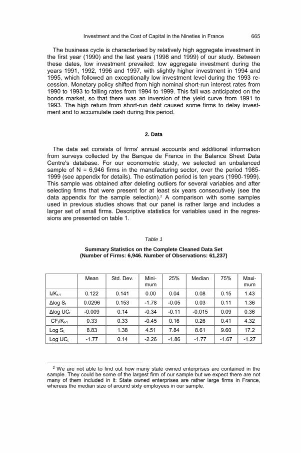
The data set consists of firms' annual accounts and additional informationfrom surveys collected by the Banque de France in the Balance Sheet DataCentre's database. For our econometric study, we selected an unbalancedsample of N = 6,946 firms in the manufacturing sector, over the period 1985-1999 (see appendix for details). The estimation period is ten years (1990-1999).This sample was obtained after deleting outliers for several variables and afterselecting firms that were present for at least six years consecutively (see thedata appendix for the sample selection).2 A comparison with some samplesused in previous studies shows that our panel is rather large and includes alarger set of small firms. Descriptive statistics for variables used in the regres-sions are presented on table 1.

Table 1

Summary Statistics on the Complete Cleaned Data Set(Number of Firms: 6,946. Number of Observations: 61,237)

Mean Std. Dev. Mini-mum

25% Median 75% Maxi-mum

It/Kt-1 0.122 0.141 0.00 0.04 0.08 0.15 1.43

∆log St 0.0296 0.153 -1.78 -0.05 0.03 0.11 1.36

∆log UCt -0.009 0.14 -0.34 -0.11 -0.015 0.09 0.36

CFt/Kt-1 0.33 0.33 -0.45 0.16 0.26 0.41 4.32

Log St 8.83 1.38 4.51 7.84 8.61 9.60 17.2

Log UCt -1.77 0.14 -2.26 -1.86 -1.77 -1.67 -1.27

2 We are not able to find out how many state owned enterprises are contained in the

sample. They could be some of the largest firm of our sample but we expect there are notmany of them included in it: State owned enterprises are rather large firms in France,whereas the median size of around sixty employees in our sample.


666

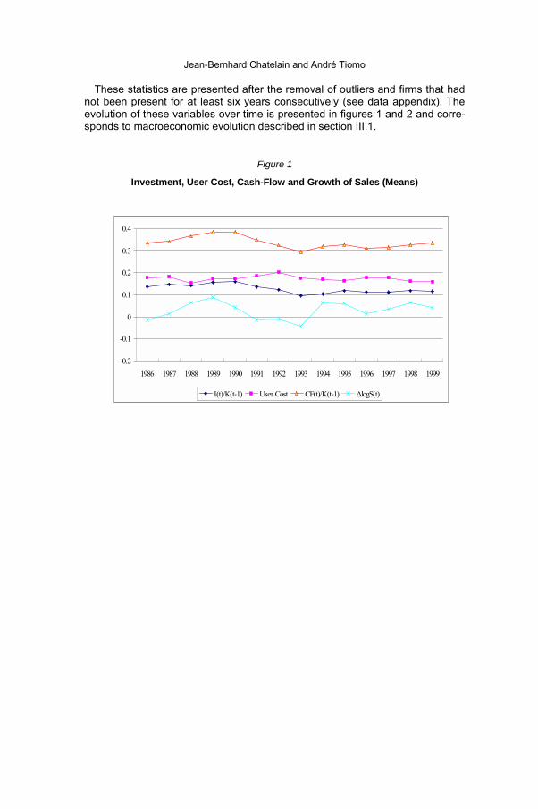
These statistics are presented after the removal of outliers and firms that hadnot been present for at least six years consecutively (see data appendix). Theevolution of these variables over time is presented in figures 1 and 2 and corre-sponds to macroeconomic evolution described in section III.1.

Figure 1

Investment, User Cost, Cash-Flow and Growth of Sales (Means)

-0.2

-0.1

0

0.1

0.2

0.3

0.4

1986 1987 1988 1989 1990 1991 1992 1993 1994 1995 1996 1997 1998 1999

I(t)/K(t-1) User Cost CF(t)/K(t-1) ∆logS(t)


667

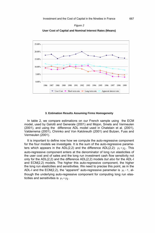
Figure 2

User Cost of Capital and Nominal Interest Rates (Means)

3. Estimation Results Assuming Firms Homogeneity

In table 2, we compare estimations on our French sample using the ECMmodel, used by Gaïotti and Generale (2001) and Mojon, Smets and Vermeulen(2001), and using the difference ADL model used in Chatelain et al. (2001),Valderrema (2001), Chirinko and Von Kalckreuth (2001) and Butzen, Fuss andVermeulen (2001).

It is important to define now how we compute the auto-regressive componentfor the four models we investigate. It is the sum of the auto-regressive parame-ters which appears in the ADL(2,2) and the difference ADL(2,2): 21 γγ + . Thisauto-regressive component enters at the denominator of long run elasticities ofthe user cost and of sales and the long run investment cash flow sensitivity notonly for the ADL(2,2) and the difference ADL(2,2) models but also for the ADL-Iand ECM(2,2) models. The higher this auto-regressive component, the higherthe long run elasticities and sensitivities. We need to precise this point, as in theADL-I and the ECM(2,2), the “apparent” auto-regressive parameter is 11 −γ , al-though the underlying auto-regressive component for computing long run elas-ticities and sensitivities is 21 γγ + .

0.00%

5.00%

10.00%

15.00%

20.00%

25.00%

1986 1987 1988 1989 1990 1991 1992 1993 1994 1995 1996 1997 1998 1999

User Cost Short term rate Long term rate Apparent interest rate

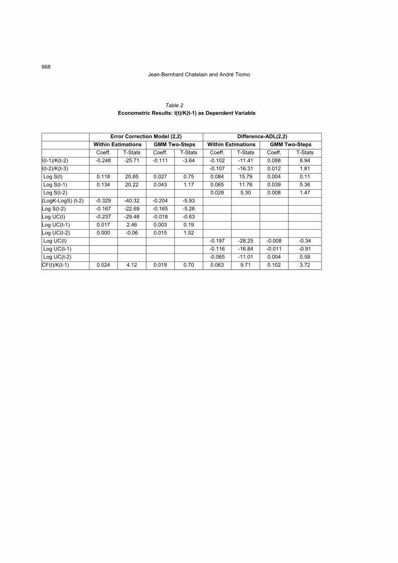
668Jean-Bernhard Chatelain and André Tiomo

Table 2Econometric Results: I(t)/K(t-1) as Dependent Variable

Error Correction Model (2,2) Difference-ADL(2,2)Within Estimations GMM Two-Steps Within Estimations GMM Two-StepsCoeff. T-Stats Coeff. T-Stats Coeff. T-Stats Coeff. T-Stats

I(t-1)/K(t-2) -0.248 -25.71 -0.111 -3.64 -0.102 -11.41 0.088 8.94I(t-2)/K(t-3) -0.107 -16.31 0.012 1.81 Log S(t) 0.118 20.85 0.027 0.75 0.084 15.79 0.004 0.11 Log S(t-1) 0.134 20.22 0.043 1.17 0.065 11.76 0.039 5.36 Log S(t-2) 0.028 5.30 0.008 1.47(LogK-LogS) (t-2) -0.329 -40.32 -0.204 -5.93Log S(t-2) -0.167 -22.69 -0.165 -5.26Log UC(t) -0.237 -29.48 -0.018 -0.63Log UC(t-1) 0.017 2.46 0.003 0.19Log UC(t-2) 0.000 -0.06 0.015 1.52 Log UC(t) -0.197 -28.25 -0.008 -0.34 Log UC(t-1) -0.116 -16.84 -0.011 -0.91 Log UC(t-2) -0.065 -11.01 0.004 0.58CF(t)/K(t-1) 0.024 4.12 0.019 0.70 0.063 9.71 0.102 3.72

669Investment and the Cost of Capital in the Nineties in France

CF(t-1)/K(t-2) 0.036 6.98 0.030 2.09 0.069 11.64 0.075 5.56

CF(t-2)/K(t-3) 0.006 1.33 -0.001 -0.10 0.044 7.82 0.0z16 2.47Auto-regressive coeff. 0.671* 0.796* -0.209* 0.100*Long term eff. Sales 0.493* 0.188* 0.146* 0.057*Long term eff. User Cost -0.669* 0.001 -0.313* -0.016Long term eff. C.-Flow 0.201 0.239* 0.146* 0.215*

AR2 -1.746p=0.081 -1.737p=0.082

Sargan 164.03p=0.133 156.27p=0.247

Estimation method: 2-step GMM estimates, time dummies and Within estimates. Instruments: lags 2 to 5 of all explanatory variables.


670

Using a Within estimator for the ECM(2,2), we find a similar result to that ob-tained by Mojon, Smets, Vermeulen (2001) who use the BACH database andomit cash-flow in their regression. The long-term user cost elasticity is very high(-0.67) and significant. Short-run elasticity is -0.24. It is interesting to see that wefind these similar results with a very high number of disaggregated observations.Part of our sample is used for constructed French data aggregated by size andsector in the BACH database. Note that the years of estimation differ betweenour study and the one by Mojon, Smets and Vermeulen (2001).

In the Within estimation for the difference ADL(2,2) model, the sum of short-run user cost elasticities is higher (-0.38) than in the ECM(2,2) model (-0.24),but the long-run user cost elasticity is now (-0.31), i.e. about half of the one withECM(2,2) (-0.67). One observes a similar decrease for long-run sales growthelasticity when shifting from the ECM model (0.493) to the difference ADL model(0.146). These differences for long-run elasticities are explained by the auto-regressive component of each model. In Within estimations, the auto-regressivecoefficient for the log of capital is 0.671 for the ECM. The explained variable inthe difference ADL model is first differences of investment/capital ratios, whichare much less auto-regressive in absolute value, and even negative (-0.209).However, the gap between investment cash-flow long-term sensitivities issmaller when shifting from the ECM model to the difference ADL model (from0.201 to 0.146). This is because the sum of short-run investment cash-flow sen-sitivities is three times higher in the difference ADL model (0.176) than in theECM model (0.066).

Using first difference GMM estimations, these auto-regressive parameters in-crease in the ECM with respect to the Within estimations, which were biaseddownwards (from 0.671 to 0.796). Due to a very low standard error, this pa-rameter is significantly different from one. The increase of the auto-regressiveparameter from Within to GMM estimator is also found in the difference ADLmodel (from -0.209 to 0.10, no longer negative). However the gap between theauto-regressive parameter of the ECM and the difference ADL remains verylarge in the GMM estimation (0.796 to 0.1). Therefore, one gets the long-run co-efficients by multiplying by 5 the sum of short-run coefficients in the ECM and bymultiplying by 1.10 the sum of short-run coefficients in the difference ADL.

Conversely, short-run coefficients of sales, user cost and cash-flow aresmaller in ECM estimations than in the difference ADL. This result goes hand inhand with the fact that the auto-regressive parameters explain much more of thevariance in the ECM model. For this reason, long-run elasticities are generallyhigher in the ECM model than in the difference ADL, if ever the short-run elas-ticities are significant. However, in both models, the user cost elasticity is notsignificantly different from zero when cash-flow and its lags are explanatoryvariables. Sales growth elasticity is significant and lower than in the Within case(where they were biased upwards). Long-term investment cash-flow sensitivitiesare slightly increased using a GMM estimation (they were biased downwardsusing Within estimates). The large differences between GMM and Within esti-mates stress endogeneity and/or heteroscedasticity problems in the Within es-timations. As the GMM estimator has been designed to deal properly with theseeconometric problems, we make no further reference to Within estimations inthe following section.


671

In Chatelain and Tiomo (2001), we check that the ECM(2,2) results are veryclose to the ADL(2,2) and ADL-I(2,2) results, where lag 2 of explanatory vari-ables (except the lag 2 of the dependant variable) are not significant and areremoved. In particular, introducing cash-flow to the regression leads to dramaticchanges in the results: User cost (and sometimes sales growth) are no longersignificant.

The result that the introduction of cash-flow drives down to zero the elasticity ofthe user cost with respect to investment (which was significant and negative be-fore the introduction of cash-flow) is robust to changes of the model: it holds forthe ADL/ECM and the difference ADL model. Not surprisingly, it is robust to thenumber of lags used in each models. It holds for other computations of the usercost such as the apparent interest rate alone, a user cost definition without taxa-tion, a user cost including more individual information related to investment taxcredit, accounting depreciation instead of a constant depreciation rate, or the “phi”parameter used by Crépon and Gianella (2001) in order to take into account in anad hoc manner the tax differentials between dividends and capital gains. It is ro-bust to soft trimming of the growth rate of the user cost (removing 1% tails of itsdistribution) or to hard trimming of the growth rate of the user cost (removing 5%tails of its distribution). It is robust to the removal of interest charges from cash-flow in order to avoid a potential collinearity problem between the apparent interestrate included in the user cost and cash-flow. It is also robust to the substitution ofcash-flow/capital by the log of liquidity (cash stock).

However, this result is not robust to data and period selection: Chatelain(2001) obtained a significant elasticity of the user cost excluding taxation on asample more or less included in the one we used in this study (a balanced panelof 4,025 firms from 1988 to 1996, estimated over the period 1993-1996). But thislast result was only obtained after strict upward testing procedures leading to theselection of highly exogenous instruments (starting from a small set of very ex-ogenous instruments and testing additional instruments one by one, see An-drews 1999). On this larger sample, a non-significant user cost was robust tosystematic changes of the instrument sets including lagged explanatory vari-ables using either upward testing procedures or downward testing procedures(starting from a large number of instrument sets and removing some of them).

4. Do Some Firms Experience a Tighter Liquidity Constraint

Why does the introduction of cash flow drive the user cost elasticity down tozero, whereas it is significantly different to zero when cash flow is omitted?

First, we define the user cost as a linear function of a microeconomic apparentinterest rate, which includes an agency premium. According to the broad creditchannel theory (see Gertler and Hubbard 1988), this agency premium decreaseswith respect to collateral, which depends on expected profits, which in turn arevery much dependant on expected sales, among other factors (for example, Olinerand Rudebush 1996 state that the agency premium increases with the risk-freeinterest rate). Due to the correlation between future profits and past profits, a po-tential explanation of the decline in the user cost elasticity, when cash flow is


672

added to the regression, may lie in the joint correlation between cash flow, salesand the apparent interest rate (hence user cost). We may face a collinearity prob-lem, which is not solved by the generalised method of moments.

A second explanation relates to an aggregation bias and to the prevalence ofself-financing during the 1990s for some firms observed in the descriptive statis-tics, both at the macroeconomic and microeconomic level: some firms may de-pend much more on cash flow than others. In that case, omitting a dummy vari-able when selecting these firms may lead to a bias in the estimate and the stan-dard error of the user cost parameter. This is what we investigate in this chapter.

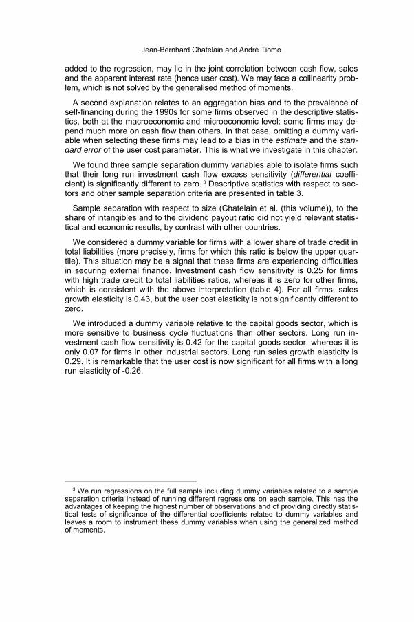
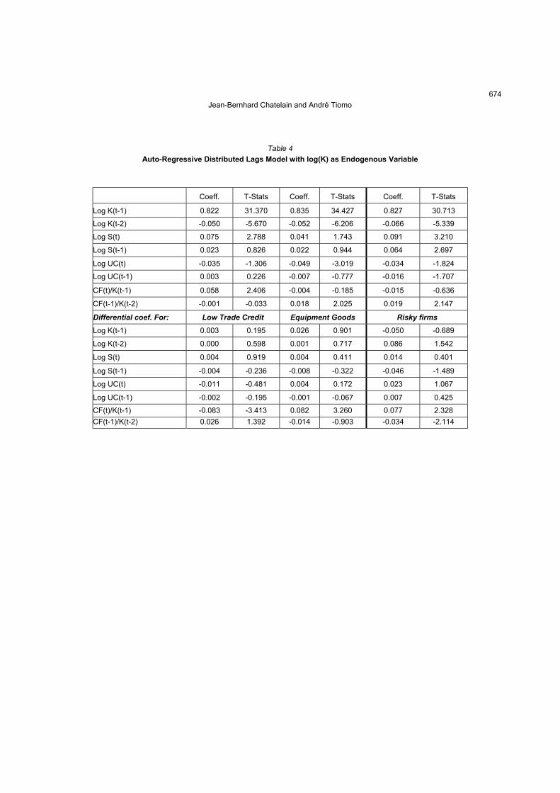
We found three sample separation dummy variables able to isolate firms suchthat their long run investment cash flow excess sensitivity (differential coeffi-cient) is significantly different to zero. 3 Descriptive statistics with respect to sec-tors and other sample separation criteria are presented in table 3.

Sample separation with respect to size (Chatelain et al. (this volume)), to theshare of intangibles and to the dividend payout ratio did not yield relevant statis-tical and economic results, by contrast with other countries.

We considered a dummy variable for firms with a lower share of trade credit intotal liabilities (more precisely, firms for which this ratio is below the upper quar-tile). This situation may be a signal that these firms are experiencing difficultiesin securing external finance. Investment cash flow sensitivity is 0.25 for firmswith high trade credit to total liabilities ratios, whereas it is zero for other firms,which is consistent with the above interpretation (table 4). For all firms, salesgrowth elasticity is 0.43, but the user cost elasticity is not significantly different tozero.

We introduced a dummy variable relative to the capital goods sector, which ismore sensitive to business cycle fluctuations than other sectors. Long run in-vestment cash flow sensitivity is 0.42 for the capital goods sector, whereas it isonly 0.07 for firms in other industrial sectors. Long run sales growth elasticity is0.29. It is remarkable that the user cost is now significant for all firms with a longrun elasticity of -0.26.

3 We run regressions on the full sample including dummy variables related to a sample

separation criteria instead of running different regressions on each sample. This has theadvantages of keeping the highest number of observations and of providing directly statis-tical tests of significance of the differential coefficients related to dummy variables andleaves a room to instrument these dummy variables when using the generalized methodof moments.


Table 3

Descriptive Statistics of Various Groups of Firms (Average Values. Number of Observations: 61,237)

Number Main Variablesof Firms I(t)/K(t-1) LogS(t) LogUC(t) CF(t)/K(t-1) LogS(t) LogUC(t)

All sectors 6946 0.122 0.0296 -0.009 0.33 8.83 -1.77Sectors Food products 929 0.12 0.01 -0.014 0.27 9.3 -1.8

Intermediate 3371 0.11 0.04 -0.005 0.29 8.8 -1.7

products

Equipment 1227 0.12 0.04 -0.008 0.37 8.7 -1.8

goodsConsumption 1286 0.15 0.01 -0.02 0.47 8.7 -1.8goods

Car industry 133 0.12 0.03 -0.02 0.31 9.8 -1.8

Scoring No score 481 0.12 0.003 0.004 0.30 9.0 -1.8

FunctionRisky Firms 1293 0.12 0.03 -0.008 0.30 8.6 -1.8

Neutral Firms 1169 0.11 0.01 -0.007 0.28 8.5 -1.7Riskness Firms 4003 0.13 0.04 -0.01 0.36 8.9 -1.8

Trade Credit < Q3 5910 0.13 0.06 -0.003 0.33 8.8 -1.8> Q3 1736 0.12 0.02 -0.011 0.33 8.8 -1.8

I/K: investment over capital; S: sales; CF/K: cash flow over capital; UC: user cost.

674Jean-Bernhard Chatelain and André Tiomo

Table 4Auto-Regressive Distributed Lags Model with log(K) as Endogenous Variable

Coeff. T-Stats Coeff. T-Stats Coeff. T-Stats

Log K(t-1) 0.822 31.370 0.835 34.427 0.827 30.713

Log K(t-2) -0.050 -5.670 -0.052 -6.206 -0.066 -5.339

Log S(t) 0.075 2.788 0.041 1.743 0.091 3.210

Log S(t-1) 0.023 0.826 0.022 0.944 0.064 2.697

Log UC(t) -0.035 -1.306 -0.049 -3.019 -0.034 -1.824

Log UC(t-1) 0.003 0.226 -0.007 -0.777 -0.016 -1.707

CF(t)/K(t-1) 0.058 2.406 -0.004 -0.185 -0.015 -0.636

CF(t-1)/K(t-2) -0.001 -0.033 0.018 2.025 0.019 2.147

Differential coef. For: Low Trade Credit Equipment Goods Risky firmsLog K(t-1) 0.003 0.195 0.026 0.901 -0.050 -0.689

Log K(t-2) 0.000 0.598 0.001 0.717 0.086 1.542

Log S(t) 0.004 0.919 0.004 0.411 0.014 0.401

Log S(t-1) -0.004 -0.236 -0.008 -0.322 -0.046 -1.489

Log UC(t) -0.011 -0.481 0.004 0.172 0.023 1.067

Log UC(t-1) -0.002 -0.195 -0.001 -0.067 0.007 0.425

CF(t)/K(t-1) -0.083 -3.413 0.082 3.260 0.077 2.328CF(t-1)/K(t-2) 0.026 1.392 -0.014 -0.903 -0.034 -2.114


Long term eff. Sales 0.43* 0.29* 0.65*

L.T. eff. User Cost -0.14 -0.26* -0.21*

L.T. eff. Cash-Flow 0.25* 0.07* 0.02*

Differential coef. For: Low Trade Credit Equipment Goods Risky firms

Long term eff. Sales 0.01 0.02 -0.04

L.T. eff. User Cost -0.06 -0.02 0.11

L.T. eff. Cash-Flow -0.25* 0.36* 0.22*

AR2 -2.266 p = 0.023 -2.077 p = 0.038 -1.993 p = 0.046

Sargan 288.22 p = 0.088 275.48 p=0.204 300.91 p = 0.031

Instruments used in the regressions are all explanatory variables lagged 2 to 5.


676

It is indeed possible that one criterion alone may not be sufficient. The “score”allocated by the Banque de France is a combination of several criteria whichmakes it possible to measure the risk of company failure. According to theBanque de France scoring system, risky firms (i.e. those whose score function isbelow -0.3) present a long run investment cash flow sensitivity of 0.24, whereasit is only 0.02 for other firms. This result was expected, as these firms experi-ence more difficulties in getting access to external financing. Sales growth elas-ticity is now 0.65. As for the capital goods sector, the user cost elasticity is sig-nificant for all firms with a long run value of -0.21.

Finally, we present the results obtained by using the risky firm dummies whenthe cash stock replaces the cash flow. For some authors, investment cash flowexcess sensitivities are not valid measures of the financing constraint (seeKaplan and Zingales 1997). One could argue that they are more likely to bevalid measures when the sample separation criterion measures, as much aspossible, the risk of bankruptcy, such as the last one we used. The stock of afirm’s cash plays the same role as the cash flow, as it is an indicator of the firm’sability to shield future investment from an expected tightening of borrowing con-ditions. The stock of cash may be less affected by the difficulty in interpreting in-vestment cash flow sensitivity, as liquidity is less likely to be a proxy of expecta-tions of future profits, which is supposed to determine investment behaviourwithout financial constraints. The stock of cash is also less correlated with salesthan cash flow, which partially removes some multicollinearity-related problemsin the investment equation.

When the stock of cash replaces the cash flow in the investment regressionand when dummy variables relative to company risk are added to the regres-sion, the user cost elasticity also becomes significant, reaching a nearly un-changed estimate of -0.23 (see table 5).

This is an additional robustness check for the user cost elasticity. The previ-ous year’s cash stock is a significant determinant of current investment, as aproportion of the previous year’s cash may finance this year’s investment. How-ever, unlike investment cash flow excess sensitivity, investment cash stock ex-cess sensitivity is not significant for more risky firms, but, at the same time, riskyfirms’ elasticity of investment with respect to sales is significantly lower than thatof other firms. This means that the investment of risky firms reacts much less tosales than that of other firms, but it could also suggest a misspecification of fi-nancial constraints in the investment equation.


677

Table 5

Auto-Regressive Distributed Lags Model with log(K)as Endogenous Variable and Cash Stock as Liquidity Variable

Coeff. T-StatsLess Risky Firms

Log K(t-1) 0.785 36.2

Log K(t-2) -0.053 -4.4

Log S(t) 0.094 3.79

Log S(t-1) 0.106 4.80

Log UC(t) -0.053 -3.01

Log UC(t-1) -0.011 -1.12

Cash(t)/K(t-1) -0.007 -0.42

Cash(t-1)/K(t-2) 0.041 2.93

Differential coef. for: Risky Firms

Log K(t-1) -0.033 -0.54

Log K(t-2) 0.055 1.10

Log S(t) 0.029 1.02

Log S(t-1) -0.091 -3.38

Log UC(t) 0.006 0.31

Log UC(t-1) 0.011 0.67

Cash(t)/K(t-1) 0.022 1.02

Cash(t-1)/K(t-2) -0.021 -1.13

Less risky firms

Long term eff. Sales 0.743*

L.T. eff. User Cost -0.238*

L.T. eff. Cash Stock 0.125*

Differential coef. For: Risky Firms

Long term eff. Sales -0.339*

L.T. eff. User Cost n.s.

L.T. eff. Cash Stock n.s.

AR2 -1.694 p = 0.090

Sargan 292.01 p = 0.066

Instruments used in the regressions are all explanatory variables lagged 2 to 5.(n.s. : not significant).


678

IV. Conclusion

We reach two major conclusions. First, by introducing sample separationdummy variables, which enable us to isolate more precisely those firms whichare more sensitive to cash flow, we improve the precision of the results pre-sented in Chatelain et al. (this volume) for France. The user cost elasticity withrespect to investment is at the most 0.26 in absolute terms for all the firms of oursample. This result is obtained using generalised method of moments estimatesfor dynamic panel data, unlike other recent papers which assess user cost ef-fects at the firm level in France. This confirms the direct effect of the interest ratechannel on investment, operating through the cost of capital.

Second, we find three groups of firms for which investment is more sensitiveto cash flow: firms facing a high risk of bankruptcy, firms belonging to the capitalgoods sector (which are more sensitive to business cycle fluctuations) and firmsmaking extensive use of trade credit, a potential substitute for short-term bankcredit. The rather high investment cash flow sensitivity of these firms (between0.24 up and 0.42), which represent about 20% of our sample, confirms the ex-istence of a broad credit channel operating through corporate investment inFrance. For other firms, investment cash flow sensitivity is close to zero.

These results offer a basis for further investigations into the effects of mone-tary policy on individual investment, and the macro-economic consequences forthe monetary transmission channels.

Summary

Using a large panel of 6,946 French manufacturing firms, this paper investigates theeffect of the cost of capital and on cash flow on investment from 1990 to 1999. We com-pare several specifications of neo-classical demand for capital, taking into account transi-tory dynamics. The user cost of capital has a significant negative elasticity with respect tocapital using traditional Within estimates, or as long as cash-flow is not added to the re-gression when using Generalised Method of Moments estimates. When dummy variablesrelated to firms more sensitive to cash flow are added in the model, the user cost elasticityis significant again and its estimate s is at most -0,26.

References

Assouline, M. et al. (1998), Stuctures et propriétés de cinq modèles macro-économiquesfrançais, Economie et Prévision 134 (3), 1–97.

Andrews, D. (1999), Consistent Moment Selection Procedures for Generalized Method ofMoments Estimation, Econometrica 67 (3), 543–564.

Angeloni, I., A. Kashyap, B. Mojon, and D. Terlizzese (2001), Monetary Transmission inthe Euro-Area, European Central Bank working paper 114.

Arrelano, M. and S. Bond (1991), Some tests of specification for panel data: Monte Carloevidence and an application to employment equation, The Review of Economic Studies58, 277–297.


679

Auerbach, A.J. (1983), Taxation, Corporate Financial Policy and the Cost of Capital,Journal of Economic Literature 21, 905–940.

Beaudu, A. and T. Heckel (2001), Le canal du crédit fonctionne-t-il en Europe? Une étudede l’hétérogénéité des comportements d’investissement à partir de données de bilanagrégées, Economie et Prévision 147, 117–141.

Blanchard, O.J. (1986), Comments and Discussion on Investment, Output and the Cost ofCapital, Brookings Paper on Economic Activity (1), 153–158.

Bond, S., J. Elston, J. Mairesse, and B. Mulkay (1997), A Comparaison of EmpiricalInvestment Equations using Company Panel Data for France, Germany, Belgium andthe UK, NBER working paper n°5900.

Butzen, P., C. Fuss and P. Vermeulen (2001), The Interest Rate and Credit Channel inBelgium: an investigation with micro-level firm data, European Central Bank workingpaper 112.

Chatelain, J.B. (2001), Investment, the Cost of Capital and Upward Testing Procedures forInstrument Selection on Panel Data, Banque de France, presented at the MonetaryTransmission meeting, March.

Chatelain, J.B. (2002), Structural Modelling of Financial Constraints on Investment: Wheredo we Stand, Paper presented at the National Bank of Belgium Conference onInvestment.

Chatelain, J.B., A. Generale, I. Hernando, P. Vermeulen, and U. von Kalckreuth (2001),Firm Investment and Monetary Transmission in the Euro Area Countries, EuropeanCentral Bank working paper 113.

Chatelain, J.B. and A. Kashyap (2000), Issues regarding estimation of the firm levelinvestment equations, European Central Bank, mimeo.

Chatelain, J.B. and J.C. Teurlai (2000a), Comparing Several Specifications of FinancialConstraints and of Adjustment Costs in Investment Euler Equation, Banque de France,presented at the European Meeting of the Econometric Society.

Chatelain, J.B. and J.C. Teurlai (2000b), Investment and the Cost of External Finance: AnEmpirical Investigation according to the Size of Firms and their Use of Leasing,Banque de France, presented at the Money, Macro and Finance conference.

Chatelain, J.B. and A. Tiomo (2001), Investment, the Cost of Capital and Monetary Policyin the Nineties in France: A Panel Data Investigation, European Central Bank workingpaper 106.

Chirinko, R., S. Fazzari, and A. Meyer (1999), How Responsive is Business CapitalFormation to its User Cost? An Exploration with Micro Data, Journal of PublicEconomics 74, 53–80.

Kalckreuth, v. Ulf (2001), Monetary transmission in Germany: New perspectives on fi-nance constraints and investment spending, Bundesbank, European Central Bankworking paper 110.

Crépon, B. and C. Gianella (2001), Fiscalité et coût d’usage du capital: incidence surl’investissement, l’activité et l’emploi, Economie et Statistique 341–342 (1/2), 107–128.

Crépon, B. and F. Rosenwald (2001), Des contraintes financières plus lourdes pour lespetites entreprises, Economie et Statistique 341–342 (1/2), 29–46.

Dormont, B. (1997), L’influence du coût salarial sur la demande de travail, Economie et deStatistique 301–302, 95–109.


680

Duhautois, R. (2001), Le ralentissement de l’investissement est plutôt le fait des petitesentreprises tertiaires, Economie et Statistique 341–342 (1/2), 47–66.

Fazzari, S.M., R.G. Hubbard, and B.C. Petersen (1988), Financing Constraint andCorporate Investment, Brookings Papers on Economic Activity, 141–195.

Gaiotti, E. and A. Generale (2001), Does Monetary Have Asymmetric Effects? A Look atthe Investment Decisions of Italian Firms, European Central Bank working paper 111.

Gertler, M. and R.G. Hubbard (1988), Financial Factors in Business Fluctuations, in:Financial Market Volatility, Federal Reserve Bank of Kanses City, 43–64.

Hall, R.E. and D.W. Jorgenson (1967), Tax Policy and Investment Behavior, AmericanEconomic Review 59 (3), 921–947.

Hall, B.H. and J. Mairesse (2001), Testing for Unit Roots in Panel Data: An ExplorationUsing Real and Simulated Data, mimeo.

Hall, B.H., J. Mairesse, and B. Mulkay (1999), Firm-level investment in France and theUnited States: an exploration of what we have learned in twenty years, Annalesd’Economie et de Statistique, 55–56.

Hall, B.H., J. Mairesse, and B. Mulkay (2000), Firm-level investment and R&D in Franceand the United States: A Comparison, Annales d’Economie et de Statistique, 55–56.

Hall, B.H., J. Mairesse, and B. Mulkay (2001), Investissement des Entreprises etContraintes Financières en France et aux Etats-Unis, Economie et Statistique, 341–342, 67–84.

Harhoff, D. and F. Ramb (2001), Investment and Taxation in Germany: Evidence fromFirm-Level Panel Data, in: Deutsche Bundesbank (ed.), Investing today for the world oftomorrow, Berlin, Heidelberg, New York: Springer.

Hayashi, F. (2000), The Cost of Capital, Q, and the Theory of Investment, in:J.L. Lau (ed.),Econometrics and the Cost of Capital, The MIT Press.

Herbet, J.B. (2001), Peut-on expliquer l’investissement à partir de ses déterminantstraditionnels au cours de la décennie 90?, Economie et Statistiques 341–342, 85–106.

Hubbard, R.G. (2000), Capital Market Imperfections, Investment, and the MonetaryTransmission Mechanism, mimeo.

Kaplan, S.N. and L. Zingales (1997), Do Investment Cash Flow Sensitivities Provide Use-ful Measures of Finance Constraints?, Quarterly Journal of Economics 112, 169–215.

King, M.A. and D. Fullerton (1984), The Taxation of Income from Capital, Chicago:Chicago University Press.

Mojon, B., F. Smets, and P. Vermeulen (2001), Investment and Monetary Policy in theEuro Area, European Central Bank working paper 78.

Oliner, S.D. and G.D. Rudebush (1994), Is there a Broad Credit Channel for MonetaryPolicy?, Working paper series. Division of Research and Statistics. Board of Governorsof the Federal Reserve System.

Valderrama, M. (2001), Credit Channel and Investment Behavior in Austria: a Micro-Econometric Approach, European Central Bank working paper 109.

Vermeulen, P. (2000), Business fixed investment: evidence of a financial accelerator inEurope, European Central Bank working paper 37.


681

Appendix

A.1. Sample Selection

The data source consists of compulsory accounting tax forms (collected bythe Banque de France in its FIBEN database) and of additional information (inparticular on leasing) taken from surveys collected by the Banque de France(the Balance Sheet Data Centre's database). These data are collected only fromfirms who are willing to provide them, a procedure which creates a bias (smallfirms of fewer than 20 employees are under-represented). No statistical sam-pling procedure has been used to correct this bias.

A first elimination of outliers was done on a larger unbalanced sample ofmanufacturing firms without holdings. Outliers were excluded using ratios builton information common to the two databases. The first step consisted in delet-ing firms with missing or inconsistent data: we selected firms with no more thanone fiscal account on the same year and for which the length of the accountingperiod was 12 months. We deleted firms for which the number of employees,sales, value added, assets, investment or debt were negative. The second stepconsisted in removing the following data:

• first percentile and the two upper percentiles of investment over capital;

• first percentile and the two upper percentiles of cash-flow over capital;

• first and 99th percentile of the apparent interest rate;

• first and 99th percentile of debt over capital;

• first and 99th percentile of sales growth;

• first percentile and the two upper percentiles of user cost;

• below the 5% percentile and above the 95% percentiles of the growthrate of the user cost.

From the initial Balance Sheet Data Centre database (209,112 initial observa-tions), we obtained an unbalanced panel of 61,237 observations i.e. 6,947manufacturing firms observed over 14 years.

A.2. Construction of the Variables

The Individual Variables

The first source is the compulsory accounting forms required under theFrench General Tax Code. These forms are completed by the firms and num-bered by the tax administration (D.G.I.) from 2050 to 2058. We provide the codeof each form omitting the first two numbers For example, we denote item FN oftax form 2050 as “(50).FN”. The second source is the Banque de France surveyof the Balance Sheet Data Centre. The form 2065 provides information onmergers and acquisitions. The form 2066 provides information on leasing. For


682

example, we denote “(cdb65).031” the item 031 of the survey form 2065. Datacommon to monetary transmission network papers are constructed according toChatelain and Kashyap’s note (2000).

Sales are total net sales (52).FL, plus the change in inventories of own pro-duction of goods and services (52).FM, plus own production of goods and serv-ices capitalised (52).FN divided by the value added deflator.

Cash flow is output ((52).FL+FM+FL+FO+FQ) minus intermediate consump-tion ((52).FS+FU+FT+FV+FW+FX) minus personal costs ((52).FY+FZ) plus netfinancial income ([52].GP-GU) minus corporate income tax ((53).HK) plus oper-ating depreciation and provisions ((52).GA+GB+GC+GD+(56)(5T-UF)).

Productive gross investment is the sum of total increases by acquisition oftangible assets (54).LP minus the sum of (i) the decreases by transfers of tangi-ble assets under construction (54).MY, and (ii) the decreases by transfers of de-posits and prepayments (54).NC minus (cdb65).031.

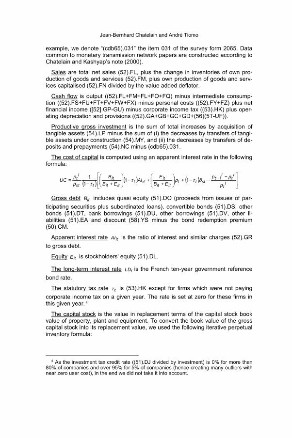
The cost of capital is computed using an apparent interest rate in the followingformula:

( ) ( ) ( )

−−−+

++−

+−= +

It

It

It

stttitit

ititt

itit

it

tst

It

p

ppEB

EAI

EBB

pp

UC 1111

1 δτρττ

Gross debt itB includes quasi equity (51).DO (proceeds from issues of par-ticipating securities plus subordinated loans), convertible bonds (51).DS, otherbonds (51).DT, bank borrowings (51).DU, other borrowings (51).DV, other li-abilities (51).EA and discount (58).YS minus the bond redemption premium(50).CM.

Apparent interest rate itAI is the ratio of interest and similar charges (52).GRto gross debt.

Equity itE is stockholders' equity (51).DL.

The long-term interest rate tLD is the French ten-year government referencebond rate.

The statutory tax rate tτ is (53).HK except for firms which were not payingcorporate income tax on a given year. The rate is set at zero for these firms inthis given year. 4

The capital stock is the value in replacement terms of the capital stock bookvalue of property, plant and equipment. To convert the book value of the grosscapital stock into its replacement value, we used the following iterative perpetualinventory formula:

4 As the investment tax credit rate ((51).DJ divided by investment) is 0% for more than

80% of companies and over 95% for 5% of companies (hence creating many outliers withnear zero user cost), in the end we did not take it into account.


683

( ) 1 1−−−= t,iitIst

Iit

it KIp

pK δ

where the investment goods deflator is denoted Istp and the depreciation rate is

taken to be 8%. The initial capital stock is given by:

ITt

KstK

st

BVit

it ppp

KK

mean000

00 with, −==

The book value of the gross capital stock of property, plant and equipmentBVitK 0 on the first available year for each firm is obtained by the sum of land

(50).AN, buildings (50).AP, industrial and technical plant (50).AR, other plantand equipment (50).AT, plant, property and equipment under construction(50).AV and payments in advance/on account for plant, property and equipment(50).AX. It is deflated by assuming that the sectoral price of capital is equal tothe sectoral price of investment meanT years before the date when the first bookvalue was available, where meanT represents the corrected average age ofcapital (this method of evaluation of capital is sometimes called the “stockmethod”). The average age of capital meanT is computed by using the sectoraluseful life of capital goods maxT and the share of goods which has been already

depreciated in the first available year in the firm's accounts )Kp/( itKst

BVit 000DEPR

( BVit0DEPR is the total book value of depreciation allowances in year 0t according

to the following formula5

.Kp

TKp

TT

,Kp

TKp

TT

itKst

BVit

itKst

BVit

itKst

BVit

itKst

BVit

8DEPR

if DEPR

21

8DEPR

if 4DEPR

00

0max

00

0maxmean

00

0max

00

0maxmean

<

=

>

−

=

The book value of depreciation allowances BVit0DEPR is obtained by the sum

of depreciation, amortisation and provisions on land (50).AO, on buildings(50).AQ, on industrial and technical plant [50].AS, on other plant and equipment(50).AU, on plant, property and equipment under construction (50).AW and onpayment in advance/on account for plant, property and equipment (50).AY.

5 This formula is used by Mairesse in the Bond et al. (1997) paper.


684

The sectoral useful life of capital goods is 15max =T years, except for sectorsC4 ( 13max =T ), sector D0 ( 16max =T ), sectors E1 and E2 ( 14max =T ), sectorE3 ( 12max =T ), and finally sector F1 ( 17max =T ).

The Sectoral Variables

We selected 5 NES16 sectors: food products, consumption goods indus-tries, equipment goods industries, intermediate products industries, and thecar industry.

Investment goods deflators Istp used for the NES16 sectors are taken from

the Annual National Accounts (base 1995).

Gross value-added deflators stp used for the NES16 sectors are taken fromthe Annual National (base 1995).

Investment and the Cost of Capital in the Nineties in ...

Documents