Invesco - Dubai

Risk & RewardResearch and investment strategies

The document is intended only for Professional Clients and Financial Advisers in Continental Europe; for Qualified Investors in Switzerland; for Professional Clients in Dubai, Ireland, the Isle of Man, Jersey and Guernsey, and the UK; for Institutional Investors in Australia; for Professional Investors in Hong Kong; for Qualified Institutional Investors, pension funds and distributing companies in Japan; for Institutional Investors and /or Accredited Investors in Singapore; for certain specific Qualified Institutions/Sophisticated Investors only in Taiwan and for Institutional Investors in the USA. The document is intended only for accredited investors as defined under National Instrument 45-106 in Canada. It is not intended for and should not be distributed to, or relied upon, by the public or retail investors.

#022nd quarter 2016

Emerging markets’ alpha beta soup

The case for factor-based investing in European equities

Long only? Long-short?

#022nd quarter 2016

Global editorial committee: Carsten Majer, Chair (Chief Marketing Officer, Invesco Continental Europe); Jutta Becker (Marketing Communications, Invesco Continental Europe); Carolyn Gibbs (Senior Strategist, Invesco Fixed Income); Dr. Jens Langewand (Managing Director – Research, Invesco Quantitative Strategies); Jonathan Peckham (Head of US Products & Marketing Research, Invesco); Florian Schwab (GPR & Product Marketing Manager, Invesco Continental Europe); Tom Tyson (Head of Product Manage ment & Investment Analysis, Invesco)Editorial deadline: 30 April 2016

Risk & Reward, Q2/2016 1

Content

Market Opportunities2 Emerging markets’ alpha beta soup

Arnab Das, Rashique Rahman, Jay RaolHow much opportunity is there to generate alpha in emerging markets (EM) fixed income? In this study we attempt to break down the drivers of returns across different EM segments into systematic and idiosyncratic factors to determine what proportion of returns is “beta” driven (systematic factors) and what portion represents opportunity for “alpha” generation (idiosyncratic factors).

5 The case for factor-based investing in European equitiesMichael FraikinBased on different MSCI style indices, the Invesco Quantitative Strategies multi-factor model, and asset manager performance we show that over the past ten years, factor investing has been particularly successful in Europe. We analyze this phenomenon in more detail and give reasons for our observations.

10 What is smart beta?Prof. Andrew Clare, Prof. Stephen Thomas, Dr. Nick MotsonIndex tracking has become ever more popular. However, in recent years, more and more investment approaches claim to provide more than a pure replication of a well-known index. In this paper, the theoretical foundations of the so-called smart-beta concept are examined.

16 Long only? Long-short?Alexander Tavernaro, Carsten RotherIf one only looks at the performance of the current constituent stocks of the established equity indices, the importance of stock picking can be easily underestimated. With the research universe of Invesco Quantitative Strategies, we aim to avoid this. On the basis of an extensive database, we highlight the importance of stock picking, explain why the damage loser stocks can cause in a portfolio is often greater than the benefits of winner stocks and discuss the potential of a long-short strategy.

Methodology19 Econometric time series models: Part 4

Dr. Bernhard PfaffThe last article in this series dealt with time series models in which the regression equation depends on the prevailing regime – as is the case with the smooth threshold autoregressive model, known as the STAR model. Here we present the statistical tests for this concept.

2 Risk & Reward, Q2/2016 Market Opportunities

We find that constituent returns across EM asset classes tend to be driven primarily by common – that is, systematic – as opposed to idiosyncratic factors, although this varies across time and asset classes. Contrary to what may be presumed, we find that EM corporate credit exhibits the highest level of systematic influence on returns over time. On average, nearly 70% of the variation in EM corporate credit constituent market returns is driven by common – not idiosyncratic, name-specific factors. In contrast, EM equities and EM duration in domestic debt are the least systematically driven; but even in these two asset classes, we find that about half of returns are explained by common global macro factors.

Our results suggest that constructing a market view on EM asset classes requires, first and foremost, a thorough understanding of top-down macro factors, followed by EM country macro analysis, complemented by bottom-up single name credit analysis. And as we will see, there will be times of transition, when these factors change places.

Two methodologiesWe utilize two methods – principal component analysis (PCA), and regression analysis – to gauge the extent of ‘beta-ness’ of EM asset classes. The ‘beta-ness’ of a market is the extent to which common factors explain the variation in returns within an asset class – in other words, the sensitivity to these common, global factors. It is the systematic component of returns. Principal component analysis (PCA) calculates the percentage of co-variation in returns for each asset class to ascertain the percentage of returns which are derived from common factors. The drawback of this approach is that the exact factors influencing returns are not known, nor are any changes in the drivers over time. However, PCA does reveal to what extent returns are influenced by systematic – as opposed to idiosyncratic – factors.

We compare the above PCA to a regression-based approach, which determines the extent of return variation explained by a predetermined set of market factors. We derive the R-squared, or explanatory power, of a regression using a set of independent variables widely used to represent each market factor against each individual asset class return. The drawback of this approach is that not all systematic components of returns may be represented; it depends on which metrics are included. That is, this approach can significantly understate the influence of common factors. This flaw becomes more serious if the systematic components of return vary over time – a problem from which PCA does not suffer.

Using PCA, Figure 1 shows the extent to which common factors drive returns across EM asset classes. They range from EM corporate credit on the high side at 68% – to EM local duration (local government bonds) and EM equity on the low side at 51%.

The regressions yield much less explanatory power for common factors than the PCA, as shown in Figure 2. Notably, EM currency displays the least ‘beta-ness’ of all asset classes by this methodology. In all likelihood, the larger influence of idiosyncratic factors implied by the regressions reflects the choice of independent variables.

Adding more variables, however, would not necessarily increase explanatory power significantly and consistently. After all, systematic risks in the global markets change rapidly. And EM economies and financial systems are constantly evolving and

Emerging markets’ alpha beta soup

How much opportunity is there to generate alpha in emerging markets (EM) fixed income? In this study we attempt to break down the drivers of returns across different EM segments into systematic and idiosyncratic factors to determine what proportion of returns is “beta” driven (systematic factors) and what portion represents opportunity for “alpha” generation (idiosyncratic factors).

Figure 1: Principal components analysis – systematic component of returns (period average, Q1/04 - Q1/16)

%

6460

51

68

51

0

20

40

60

80

Sovereign credit

Local currency

Local duration

Corporate credit

Equity

Source: Invesco, data from 9 January 2004 to 11 March 2016. Sovereign credit is represented by constituents of the JPMorgan EMBI Global Diversified Index. Local currency is represented by spot currencies, data from Bloomberg L.P. Local duration is represented by constituents of the JPMorgan GBI-EM Broad USD Hedged Index. Corporate credit is represented by constituents of the JPMorgan CEMBI Broad Diversified Index. Equity is represented by the MSCI EM USD Hedged Index.

Figure 2: Regression analysis – systematic component of returns (period average, Q1/04 - Q1/16)

%

41

15

23

46

33

0

10

20

30

40

50

Sovereign credit

Local currency

Local duration

Corporate credit

Equity


Risk & Reward, Q2/2016 3 Market Opportunities

integrating into global markets. Some of these changes would increase exposure to common factors; others would reduce such exposure; yet others would change the key factors, systematic or idiosyncratic.

Indeed, another important result is that the influence of systematic factors, regardless of method, varies considerably over time. As Figure 3 demonstrates, in the case of EM equities, for example, using PCA, we can see that the influence of common factors has been as low as 30% and as high as 70% over the last decade. Therefore, idiosyncratic factors do have major influence at times on market outcomes – though not on average.

A question of global financial integrationWhat explains the differences in systematic influence across EM asset classes? Broadly across the two methods, our results tell a similar story – the more globally integrated the EM asset class, the greater the role of systematic factors in influencing returns; the less integrated, the greater the potential for idiosyncratic factors to influence returns.

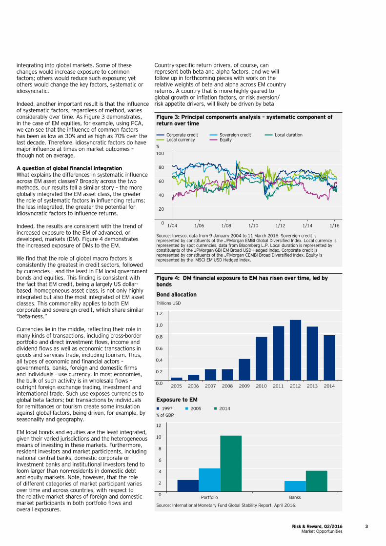
Indeed, the results are consistent with the trend of increased exposure to the EM of advanced, or developed, markets (DM). Figure 4 demonstrates the increased exposure of DMs to the EM.

We find that the role of global macro factors is consistently the greatest in credit sectors, followed by currencies – and the least in EM local government bonds and equities. This finding is consistent with the fact that EM credit, being a largely US dollar-based, homogeneous asset class, is not only highly integrated but also the most integrated of EM asset classes. This commonality applies to both EM corporate and sovereign credit, which share similar “beta-ness.”

Currencies lie in the middle, reflecting their role in many kinds of transactions, including cross-border portfolio and direct investment flows, income and dividend flows as well as economic transactions in goods and services trade, including tourism. Thus, all types of economic and financial actors – governments, banks, foreign and domestic firms and individuals - use currency. In most economies, the bulk of such activity is in wholesale flows – outright foreign exchange trading, investment and international trade. Such use exposes currencies to global beta factors; but transactions by individuals for remittances or tourism create some insulation against global factors, being driven, for example, by seasonality and geography.

EM local bonds and equities are the least integrated, given their varied jurisdictions and the heterogeneous means of investing in these markets. Furthermore, resident investors and market participants, including national central banks, domestic corporate or investment banks and institutional investors tend to loom larger than non-residents in domestic debt and equity markets. Note, however, that the role of different categories of market participant varies over time and across countries, with respect to the relative market shares of foreign and domestic market participants in both portfolio flows and overall exposures.

Country-specific return drivers, of course, can represent both beta and alpha factors, and we will follow up in forthcoming pieces with work on the relative weights of beta and alpha across EM country returns. A country that is more highly geared to global growth or inflation factors, or risk aversion/risk appetite drivers, will likely be driven by beta

Figure 4: DM financial exposure to EM has risen over time, led by bonds

Bond allocationTrillions USD

0.0

0.2

0.4

0.6

0.8

1.0

1.2

2005 2006 2007 2008 2009 2010 2011 2012 2013 2014

Exposure to EM• 1997 • 2005 • 2014% of GDP

0

2

4

6

8

10

12

Portfolio Banks

1997 2005 2014

Source: International Monetary Fund Global Stability Report, April 2016.

Figure 3: Principal components analysis – systematic component of return over time

Corporate credit Sovereign credit Local duration Local currency Equity

%

0

20

40

60

80

100

1/04 1/06 1/08 1/10 1/12 1/14 1/16

Sovereign Credit Local Currency Local Bond (Hedged)

Corporate Credit Equity



more than alpha relative to a more closed economy. Thus, small or open EM economies whose business and financial cycles are commodity dominated will tend to be much higher beta than more isolated EM economies, even those that are similar in terms of income levels or financial development.

Finally, policy can make a major difference, overcoming structural or geographic features – but only up to a point. A small, resource-rich or otherwise trade-heavy economy with a relatively small population will tend to be dominated by global commodity and growth/inflation cycles; such features are very difficult to change (for example, Ecuador) but policies that encourage savings and the accumulation of precautionary official reserves of private foreign assets can help cushion cyclical shifts and beta (for example, Singapore or Chile).

On the other hand, high reliance on cross-border portfolio capital flows and financial markets can render even a relatively large, diversified economy with modest trade exposures heavily exposed to global financial conditions and thereby, a high-beta country (for example, Brazil or Russia). A large closed but high-deficit country would be high beta, but through external, fiscal/monetary and structural adjustment can reduce exposure to global macro factors and risks (for example, India from 2013-14/15).

The overall framework of policies across countries can also make a major difference. Many EM countries have moved from fixed exchange rates mainly against the dollar (which effectively limited their monetary policy freedom) toward managed floats with inflation targeting (which means that currencies now act as the main economic shock absorber, rather than interest rates, allowing central banks much greater autonomy to set interest rates).

These changes in the typical EM macro policy regime imply shifts in the degree of systematic influence across asset classes. When exchange rates were fixed, traded in corridors or in crawling pegs, currencies would not adjust to external shocks – at least not initially, and usually not until severe pressures had accumulated. Instead, the size of central bank balance sheets and domestic interest rates would respond to global trade and capital flows. The financial and economic logic underlying this result strongly suggests that this phenomenon will continue, maintaining the rank order of “beta-ness” across asset classes, amid variability.

Gauging macro (high-level) risk – how we integrate the approach The above results tie directly into our analytical framework and our investment process. We start with the fact that top-down global macro trends tend to dominate bottom-up country-specific factors in driving excess returns. Put another way, on average, we believe that having the right EM country or credit (idiosyncratic or alpha) view will not save the

performance of an EM investment portfolio that is constructed with an inappropriate sensitivity to ‘common’ (systematic) factors. Assessing the direction and level of systematic risk, or beta, to these risk factors, is crucial, in our view, in calibrating risk appropriately in portfolios, given that these macro (high-level) risks will tend to be the key determinants of portfolio performance.

We believe having the right bottom-up, idiosyncratic view can substantially enhance returns in a portfolio that is appropriately oriented to common global macro ‘beta’ factors. We also believe the uncertainty and variability in the weights of systematic and idiosyncratic factors in explaining returns calls for complementing top-down with bottom-up analysis.

As such, as part and parcel of our process, we continuously assess the extent to which common factors are driving asset returns. This allows us to calibrate the extent of ‘beta-ness’ we wish to represent in our portfolios. This, as we have seen, varies across strategies, depending on whether it is credit or local currency, for example.

Furthermore, we take active views on common factors that tend to influence market directionality. We believe this provides us with greater scope to appropriately gauge the extent of macro risk prevalent within our portfolios.

We then place EM country and single-name analysis within this beta framework. This approach enables us to focus our analysis on specific cases where a bottom-up narrative can generate alpha, even in the context of the beta view.

In forthcoming pieces, we will 1) seek to quantify the influence of alpha and beta in driving excess returns at country level; and 2) compare the “beta-ness” of EM against other asset classes as well as consider the impact of sector-level beta factors in EM corporate credit returns.

Arnab Das, Head of Emerging Markets Macro Research Rashique Rahman, Head of Emerging Markets Jay Raol, Senior Macro Analyst Invesco Fixed Income

Notes1 The independent variables used in the regression are the S&P

500 index, US 10-year yield, VIX Index, EUR/USD exchange rate, Bloomberg Commodity Index, Barclays High Yield Spread Index, Citi Developed Market Growth Surprise Index of G10 and Citi Developed Market Inflation Surprise Index of G10. The Citi Surprise Growth Index tracks the data releases pertaining to real growth of the major economies against economist expectations. A large negative number represents economic data that has come in below economist expectations. The Citi Surprise Inflation Index tracks the data releases pertaining to inflation of the major economies against economist expectations. A large negative number represents economic data that has come in below economist expectations.

2 IMF Global Financial Stability Report, April 2014.


In this article we explore whether European equity markets are particularly amenable to factor-based investing by examining several pieces of evidence: factor-based style indices, the proprietary Invesco Quantitative Strategy (IQS) multi-factor model and asset manager performance. Naturally in all of this we do not only need Europe market data – we also need something to compare it with. Whilst it would be tempting to analyze all regions on an equal footing, this would in practice be difficult to achieve as evidence is either unavailable or hard to compare fairly for at least some of the regions. We have therefore decided to focus on Europe versus the World and derive our conclusions from this. Many will now be pondering what we actually mean by factor-based investing and, indeed, this is a question without a definitive answer as no common definition exists as yet. Broadly speaking the factors we are looking for can be defined quantitatively and are expected to explain consistently parts of the return and risk profiles of securities. For our purposes we will consider “classic” factors such as Value and Momentum and also newer arrivals such as Low Volatility. Whilst for some market participants, simple and transparent factors are part and parcel of factor-based investing we shall, when we move beyond the style indices, also allow for factors and factor-based investing that rely on more complex definitions of factors and allow for more advanced methods of portfolio construction. The question of single-factor versus multi-factor approaches will not be tackled directly in this context. However, we believe that multi-factor approaches conceptually dominate single factor approaches.

European and global style indicesHere we compare the relative performance of European and Global Style indices as evidence of the suitability of factor-based approaches for European equities. We base our analysis on MSCI indices that have mostly been launched in the last decade – a family that continues to expand with the evolving requirements of investors. Naturally our analysis is qualified – most of the MSCI indices have been created comparatively recently, and therefore, contain elements of hindsight as well as a selection bias. Indices are defined for particular factors and employ a method that would have worked in the past. The first style indices that MSCI introduced were Value and Growth (European and World launched in 1997), which split the entire universe into two buckets representing roughly the same market capitalization based on value and growth criteria, with all index constituents of the standard index either fully allocated to Value or Growth or partially to both – but with no securities unallocated. The newer style indices are different from the first incarnation in that they do not aim to include a set proportion of the market capitalization and they have potentially overlapping constituents and weighting schemes that can differ from market capitalization. The newer tilted indices (not reflected

in table 1) have been created realizing the liquidity needs of investors and taking investability more strongly into account.

Table 1 shows the return and risk figures for a broad selection of Global and European style indices relative to their respective capitalization weighted indices that we use as evidence of the amenability of the European and Global equity markets to factor-based investing. When comparing Europe with the world we should bear in mind that, given the broader universe, Global should theoretically deliver lower risk and better return/risk figures if the underlying success of the factors is the same. We therefore focus more strongly on the relative return figures. Momentum and Quality evidence a noticeably stronger relative performance in Europe than in the World over the last 10 years, reverting during the prior ten years. Value-related factors are clearly a puzzle – evidenced by the plethora of indices, none of which delivered compelling returns in Europe over the last 10 years. In most cases Value indices failed to generate excess returns over the last ten years, reverting to a strong return to value up to 2007. Small size (Small Cap and Equal Weighted) did broadly well and better in Europe with the Equal Weighted indices flattening out over the last ten years. Small Caps stood out in Europe in particular. Risk continued to underperform with both Minimum Volatility and the Risk Weighted indices outperforming and Minimum Volatility doing particularly well. Looking at the Risk Weighted indices, Europe dominated over the last five years but not over longer periods. Growth as the final category made an unlikely comeback over the last few years – given that it is basically the opposite of Value – and strongly outperformed over recent history, especially in Europe. In summary it is fair to say that over the last ten years style indices in aggregate did better in Europe although this cannot be concluded over the last 20 years. This bodes well

The case for factor-based investing in European equities

Based on different MSCI style indices, the Invesco Quantitative Strategies multi-factor model, and asset manager performance we show that over the past ten years, factor investing has been particularly successful in Europe. We analyze this phenomenon in more detail and give reasons for our observations.

Executive summary

• This paper compares the potential for success in European versus global equity markets of investment approaches based on quantitatively measured attributes (factors).

• Over the last 10 years, European style indices in the aggregate – and momentum and quality indices in particular – have outperformed comparable global style indices. Similarly, over this same time period managers employing quantitative strategies focused on European stocks outperformed quantitative managers with a global equity focus.

• Performance dispersion among individual factors has been greater for European indices than global indices.

• Over the last 10 years, the proprietary, multi-factor model used by Invesco Quantitative Strategies exhibited significantly greater differentiation between top and bottom quintile and 1st and 2nd quintile performance for European stocks versus global stocks.

• European stocks may be more amenable to a quantitative, factor-based investing approach due to the relative inefficiency of European stock markets compared to U.S. markets.


for further outperformance of Europe if Value factors continue to be mean reverting in their long-term relative performance whereas Momentum factors have tended to trend.

Figures 1 and 2 allow us to have a look at the evolution of the relative returns of a number of style indices. The World and Europe naturally exhibited similarities but also showed some differences. The global picture showed fewer clear trends over the last years than previously and the European picture showed clearer trends across the years – especially leading up to 2007. What may be less obvious but still noteworthy is the fact that the span of factor differentiation has tended to be bigger in Europe (i.e. European factors have had more strongly differentiated performance). The only prolonged

period for which this was not the case was for the years 1998 and 1999.

Figure 3 looks at the European versus the Global relative performance of selected factors. We can see that the relative performance for the factors that have 20 years of history has been very similar – whilst for those with shorter histories (Minimum Volatility and Small Caps) Europe has outperformed the World. The first five years of the chart show the relative outperformance of the World followed by sideways movements for some factors and European outperformance for others up to the financial crisis and then the majority of European factors outperforming. Value has led a life of its own and its evolution in this context was actually negatively correlated to that of many other styles

Table 1: Return and risk MSCI index figures

Metric Return (%) Risk (%) Return/risk

Years 1 3 5 10 20 1 3 5 10 20 1 3 5 10 20

Absolute

Capitalization WeightedEurope 3/1986 -2.80 4.50 3.90 3.40 6.30 14.80 13.70 16.70 21.70 18.20 N-M 0.33 0.23 0.16 0.35World 3/1986 -0.90 9.60 7.60 5.00 6.00 13.30 10.80 12.70 17.50 15.40 N-M 0.89 0.6 0.28 0.39

Relative

MomentumEurope 12/2013 5.80 3.80 4.10 4.10 6.80 4.80 4.80 5.70 7.50 8.20 1.2 0.78 0.72 0.54 0.83World 12/2013 5.00 2.90 3.50 1.70 6.80 3.90 4.40 5.60 7.30 8.10 1.29 0.67 0.62 0.23 0.84

QualityEurope 12/2012 6.40 2.80 3.90 3.70 5.60 3.70 3.80 4.80 6.20 5.80 1.73 0.74 0.81 0.59 0.97World 12/2012 4.60 2.70 3.10 3.10 6.00 2.70 2.50 3.40 4.30 4.50 1.69 1.11 0.89 0.71 1.31

Value

Europe 12/1997 -7.00 -2.40 -1.90 -2.20 0.10 2.00 2.70 3.30 4.20 4.10 N-M N-M N-M N-M 0.03

World 12/1997 -4.00 -1.80 -1.10 -1.10 -0.20 1.60 1.70 2.00 2.80 3.70 N-M N-M N-M N-M N-M

Value WeightedEurope 12/2010 -4.70 -1.70 -2.10 -1.50 0.00 2.60 2.80 3.40 4.20 3.50 N-M N-M N-M N-M N-MWorld 12/2010 -3.30 -1.60 -1.60 -0.90 1.20 1.80 1.60 2.10 2.90 3.30 N-M N-M N-M N-M 0.37

Enhanced IndexEurope 9/2014 -3.80 -1.10 -1.90 -0.70 n/a 3.00 3.50 4.00 4.30 n/a N-M N-M N-M N-M n/aWorld 8/2014 -0.40 5.10 2.10 1.90 n/a 4.60 4.90 4.90 5.10 n/a N-M 1.05 0.43 0.36 n/a

High DividendEurope 10/2006 -0.50 1.30 0.90 -0.80 2.60 2.80 3.30 4.90 5.20 5.60 N-M 0.39 0.18 N-M 0.46World 10/2006 -2.40 -2.80 -0.40 -0.50 2.60 3.30 3.30 4.30 4.90 5.80 N-M N-M N-M N-M 0.45

Small CapEurope 1/2001 14.10 8.20 4.30 3.80 n/a 5.30 5.40 6.00 8.30 n/a 2.65 1.52 0.71 0.46 n/aWorld 1/2001 0.60 0.70 -0.10 1.00 n/a 4.80 5.00 4.60 5.60 n/a 0.12 0.14 N-M 0.18 n/a

Equal WeightedEurope 1/2008 2.30 1.30 -0.40 0.20 1.80 1.20 2.00 2.90 4.50 5.10 1.92 0.64 N-M 0.04 0.36

World 1/2008 -0.60 -1.00 -1.50 0.20 1.70 2.20 2.10 2.20 3.50 5.10 N-M N-M N-M 0.05 0.33

Minimum Volatility*Europe 9/2009 7.40 4.50 4.50 2.70 n/a 4.80 4.40 5.60 6.40 n/a 1.55 1.02 0.81 0.43 n/aWorld 8/2008 6.10 1.80 2.20 1.50 2.60 6.60 6.00 7.70 8.00 7.30 0.93 0.29 0.29 0.18 0.36

Risk WeightedEurope 5/2011 3.50 2.20 1.40 1.40 3.60 1.90 2.10 2.30 3.00 4.60 1.8 1.06 0.61 0.46 0.78World 4/2011 0.30 -0.40 -0.20 1.10 3.90 2.40 2.90 3.30 3.30 5.30 0.14 N-M N-M 0.33 0.74

GrowthEurope 12/1997 7.00 2.20 1.70 2.10 -0.50 1.90 2.70 3.20 4.00 4.10 3.78 0.83 0.54 0.53 N-MWorld 12/1997 4.00 1.70 1.10 1.10 -0.30 1.50 1.70 2.00 2.80 3.80 2.59 1.03 0.55 0.39 N-M

* Minimum Volatility is based on the USD based indices. EUR based indices were launched in 2011.Source: MSCI for the index series and Invesco for the calculations as of 31 December 2015. All figures in USD. N-M means not numerically meaningful. n/a means no data available (some indices have not been calculated back 20 years). Past performance is not a guarantee of future results. An investment cannot be made in an index.


(Momentum, Quality and Minimum Volatility). This means that when Value did better in the World than in Europe the other factors were likely to have done better in Europe and vice versa.

The Invesco Quantitative Strategy (IQS) Stock Selection ModelAnother piece of evidence we consider here is the performance of the IQS stock selection model as it has evolved over time. IQS has built quantitative models since 1983 – initially for the US market but also since 1999 for European and 2001 for global markets. IQS uses a multi-factor model that has been adapted to take regional market idiosyncrasies into account across the world. The IQS model has four concepts: Earnings Expectations (looking largely for estimate revisions and earnings surprises), Market Sentiment (primarily focused on medium-term price trend but also covering short interest and short-term reversal factors), Management & Quality (growth, leverage, usage of capital and other items related to corporate behavior and management) and Value (most

importantly cash flow yield but also earnings and dividend yield) – with the first two predominantly Momentum-related and the other two conceptually closest to Quality and Value. While factors such as size or volatility are not part of the IQS factor model, they are built into portfolios at the portfolio construction stage when deemed appropriate.

Given that Europe is an important component of the model (actually comprising two regions: the UK and Continental Europe) but not the dominant focus of the team, we believe it is fair to use the IQS model as evidence of the suitability of factor-based approaches to the European markets. What should be noted, however, is that unlike the previous analysis, in which the factors used were effectively plain vanilla and non-proprietary, the factors of the IQS model are more complex and proprietary. A clear advantage in our analysis was, however, the fact that we could use actual data for the IQS models as they evolved rather than back-testing the current model.

We used two sets of information to help us explore this issue: information coefficients and quintile spreads. Information coefficients were determined using historic factor scores and correlated to subsequent one-month returns. In figure 4 and 5, we look at a cumulative series of these monthly results. The quintile spreads represent the relative performance of the buckets with the 20% most (Q1) and least (Q5) attractive securities in our universes. They were sorted every month and the stocks weighted by market capitalization.

Whilst the broad patterns for Europe and the World resemble each other, there are some notable differences. In the European model the differentiation between the first (most attractive) quintile and the second was much larger than in the World model and the relative performance of the first and last quintile was more extreme in the European model. In both cases there was no meaningful differentiation for quintiles three and four, the gap between quintile one and five generally expanded and the relative underperformance of quintile five exceeded the outperformance of quintile one.

Figure 1 and 2: MSCI style indices versus capitalization weighted indices

Enhanced Value Equal Weighted Growth High Dividend Minimum Volatility Momentum Quality Risk Weighted Small Caps Value Value Weighted

European factors World factors

20

40

60

80

100

120

140

1/96 1/01 1/06 1/11

Enhanced Value Equal Weighted Growth High DividendMinimum VolatilityMomentum Quality Risk WeightedSmall Caps Value Value weighted

20

40

60

80

100

120

140

1/96 1/01 1/06 1/11

Enhanced Value Equal Weighted Growth High DividendMinimum VolatilityMomentum Quality Risk WeightedSmall Caps Value Value weighted

Source: MSCI for the index series and Invesco for the calculations as of 31 December 2015. All figures in USD. The charts show the performance of European and World style indices relative to their respective capitalization-weighted indices, respectively; data rebased to 100 at 31 December 2015 and calculated back as far as index data is available. Past performance is not a guarantee of future results. An investment cannot be made in an index.

Figure 3: Relative performance of MSCI style indices – Europe versus the World

Growth Momentum Small Caps Minimum Volatility Quality Value

60

70

80

90

100

110

120

1/96 1/01 1/06 1/11

Growth Minimum VolatilityMomentumQuality Small Caps Value

Source: MSCI for the index series and Invesco for the calculations as of 31 December 2015. All figures in USD. Figure 3 shows performance of European and World style indices relative to each other; data rebased to 100 at 31 December 2015. Past performance is not a guarantee of future results. An investment cannot be made in an index.


Figure 6 delivers an interesting insight. From 2005 to 2008, the difference between the Global and the European model in separating attractive and unattractive was negligible – both did a roughly equal job with Europe starting stronger but underperforming relative to the World in the 2008. After 2008, Europe outperformed the World – initially in Q1 and Q5 from 2012 onwards only in Q1 – meaning that the model did as well in Europe as in the World in identifying the unattractive securities but did even better at identifying the attractive equities.

The analysis of the cumulative information coefficients (IC) allows us to shed more light on our question. Figure 7 shows the cumulative IC evolution for the European and the Global model. The pattern is similar to that exhibited by the quintile spreads. Europe and the World trended up 2005 to approximately 2008, suffered a setback and then resumed their upward trajectory which was, however, more pronounced for Europe.

Figure 8 allows additional analysis. We can see that the fairly steady advantage for Europe since 2009 was largely driven by Earnings Expectations – which continued to shine in Europe, Management & Quality and Value whereas Market Sentiment performed equally well in Europe and the World. The relative

performance of our European Value concept was somewhat in contrast to the picture from the style indices. This can be plausibly explained by the fact that our most important value driver was cash flow yield which did not suffer the same poor

Figure 4 and 5: IQS quintile spreads

Q1 Q2 Q3 Q4 Q5

Europe World

40

60

80

100

120

140

160

5/05 5/07 5/09 5/11 5/13 5/15

Q1 Q2 Q3 Q4 Q5

60

70

80

90

100

110

120

130

5/05 5/07 5/09 5/11 5/13 5/15

Q1 Q2 Q3 Q4 Q5

Source: Invesco as of 31 December 2015. Figure 4 and 5 show the quintile performance of the IQS European and World models, respectively. Our universes currently consist of around 1000 (Europe) and 4000 securities (World).

Figure 6: IQS quintile spreads – Europe versus world

Q1 Q5

60

70

80

90

100

110

120

130

5/05 5/07 5/09 5/11 5/13 5/15

Q1 Q5

Source: Invesco as of 31 December 2015. Performance of the IQS European and World models’ quintiles relative to each other.

Figure 7: IQS European and global information coefficients – total alpha

Europe World

-1

0

1

2

3

4

5/05 5/07 5/09 5/11 5/13 5/15

Europe World

Source: Invesco as of 31 December 2015. Cumulative information coefficients of the IQS European and the IQS World model (total alpha).

Figure 8: IQS European versus global information coefficients

Earning Expectations Management & Quality Total Alpha Market Sentiment Value

-2

-1

0

1

2

5/05 5/07 5/09 5/11 5/13 5/15

Earnings ExpectationsMarket SentimentManagement & Quality

Value Total Alpha

Source: Invesco as of 31 December 2015. Cumulative information coefficients of the IQS European model relative to the IQS World model.


performance that most value metrics did over the period since 2009.

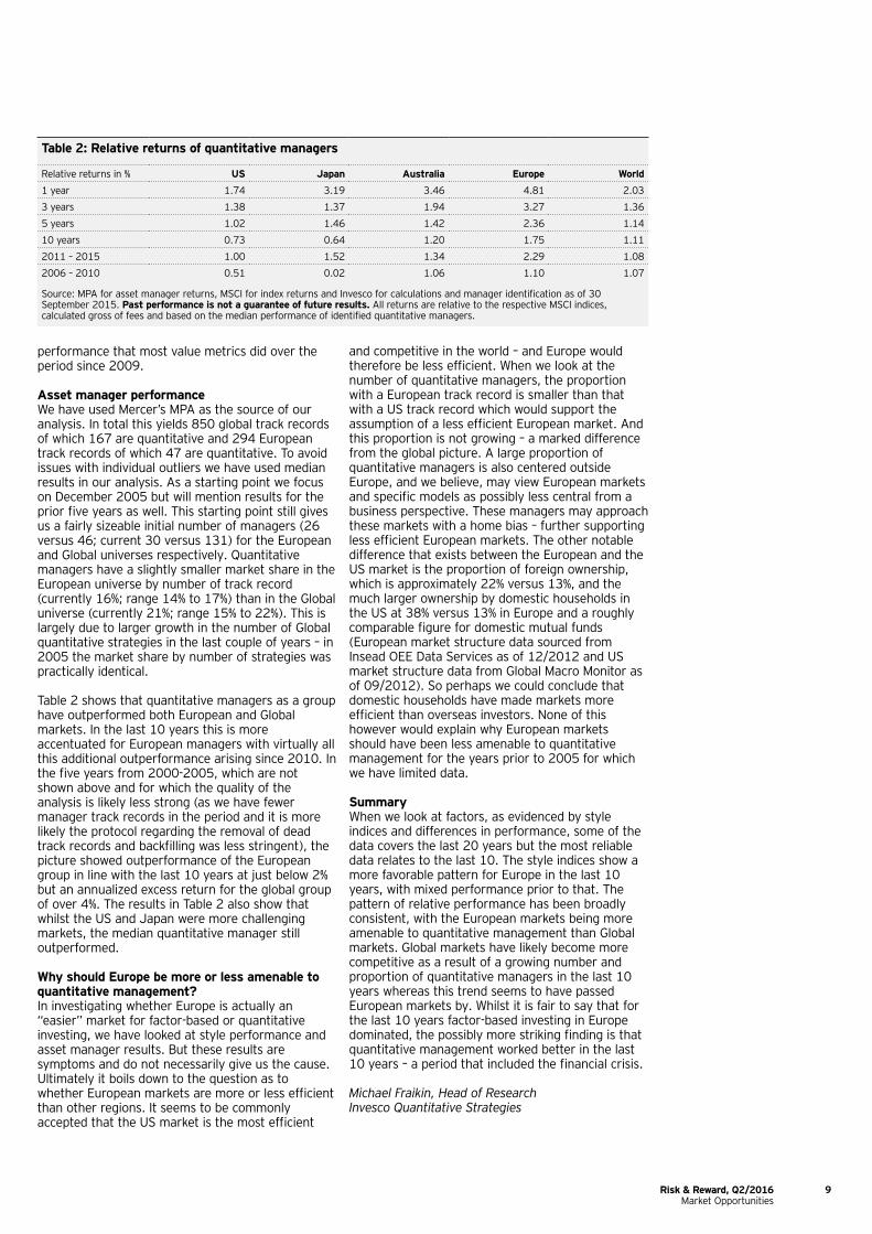
Asset manager performanceWe have used Mercer’s MPA as the source of our analysis. In total this yields 850 global track records of which 167 are quantitative and 294 European track records of which 47 are quantitative. To avoid issues with individual outliers we have used median results in our analysis. As a starting point we focus on December 2005 but will mention results for the prior five years as well. This starting point still gives us a fairly sizeable initial number of managers (26 versus 46; current 30 versus 131) for the European and Global universes respectively. Quantitative managers have a slightly smaller market share in the European universe by number of track record (currently 16%; range 14% to 17%) than in the Global universe (currently 21%; range 15% to 22%). This is largely due to larger growth in the number of Global quantitative strategies in the last couple of years – in 2005 the market share by number of strategies was practically identical.

Table 2 shows that quantitative managers as a group have outperformed both European and Global markets. In the last 10 years this is more accentuated for European managers with virtually all this additional outperformance arising since 2010. In the five years from 2000-2005, which are not shown above and for which the quality of the analysis is likely less strong (as we have fewer manager track records in the period and it is more likely the protocol regarding the removal of dead track records and backfilling was less stringent), the picture showed outperformance of the European group in line with the last 10 years at just below 2% but an annualized excess return for the global group of over 4%. The results in Table 2 also show that whilst the US and Japan were more challenging markets, the median quantitative manager still outperformed.

Why should Europe be more or less amenable to quantitative management?In investigating whether Europe is actually an “easier” market for factor-based or quantitative investing, we have looked at style performance and asset manager results. But these results are symptoms and do not necessarily give us the cause. Ultimately it boils down to the question as to whether European markets are more or less efficient than other regions. It seems to be commonly accepted that the US market is the most efficient

and competitive in the world – and Europe would therefore be less efficient. When we look at the number of quantitative managers, the proportion with a European track record is smaller than that with a US track record which would support the assumption of a less efficient European market. And this proportion is not growing – a marked difference from the global picture. A large proportion of quantitative managers is also centered outside Europe, and we believe, may view European markets and specific models as possibly less central from a business perspective. These managers may approach these markets with a home bias – further supporting less efficient European markets. The other notable difference that exists between the European and the US market is the proportion of foreign ownership, which is approximately 22% versus 13%, and the much larger ownership by domestic households in the US at 38% versus 13% in Europe and a roughly comparable figure for domestic mutual funds (European market structure data sourced from Insead OEE Data Services as of 12/2012 and US market structure data from Global Macro Monitor as of 09/2012). So perhaps we could conclude that domestic households have made markets more efficient than overseas investors. None of this however would explain why European markets should have been less amenable to quantitative management for the years prior to 2005 for which we have limited data.

SummaryWhen we look at factors, as evidenced by style indices and differences in performance, some of the data covers the last 20 years but the most reliable data relates to the last 10. The style indices show a more favorable pattern for Europe in the last 10 years, with mixed performance prior to that. The pattern of relative performance has been broadly consistent, with the European markets being more amenable to quantitative management than Global markets. Global markets have likely become more competitive as a result of a growing number and proportion of quantitative managers in the last 10 years whereas this trend seems to have passed European markets by. Whilst it is fair to say that for the last 10 years factor-based investing in Europe dominated, the possibly more striking finding is that quantitative management worked better in the last 10 years – a period that included the financial crisis.

Michael Fraikin, Head of Research Invesco Quantitative Strategies

Table 2: Relative returns of quantitative managers

Relative returns in % US Japan Australia Europe World

1 year 1.74 3.19 3.46 4.81 2.03

3 years 1.38 1.37 1.94 3.27 1.36

5 years 1.02 1.46 1.42 2.36 1.14

10 years 0.73 0.64 1.20 1.75 1.11

2011 – 2015 1.00 1.52 1.34 2.29 1.08

2006 – 2010 0.51 0.02 1.06 1.10 1.07

Source: MPA for asset manager returns, MSCI for index returns and Invesco for calculations and manager identification as of 30 September 2015. Past performance is not a guarantee of future results. All returns are relative to the respective MSCI indices, calculated gross of fees and based on the median performance of identified quantitative managers.


1. IntroductionWhile the advent of the modern stock market index is usually traced to the creation of the Dow Jones Industrial Average in 1896, it was the pioneering asset pricing work some 60 years later of Harry Markowitz1 who introduced the world to the phrase ‘Modern Portfolio Theory’ in the 1950’s and the work of Eugene Fama2 which introduced the investment world to the notion of the Efficient Market Hypothesis (EMH) that essentially formed the intellectual basis for a style of investing that has become known invariably as ‘passive investing’ or ‘index tracking’. Subsequently Burton Malkiel3 and Charles Ellis4 each wrote forcefully about the case for investing in line with financial market indices that were calculated on a market capitalisation-weighted basis as an alternative to investing with an ‘active’ fund manager.

With this intellectual firepower behind it, index tracking as an approach to investing has grown dramatically over the past forty years. The first institutional funds designed specifically to track a market cap-weighted equity index were created in 1973, these were closely followed in 1976 by the launch of the first index mutual fund by Vanguard. Today passive, or to be more precise, index tracking investment vehicles are widely available, both to institutional investors, and to retail investors. According to the ICI 2015 Factbook5 in North America USD17.9trn was invested in mutual at the end of 2014; of this total just over USD2.0trn was invested in indexed mutual funds, up from USD27.8bn at the end of 1993. According to the Investment Association’s Annual Survey of the UK’s fund management industry, 20% of total UK assets under management were managed on a “fully passive” basis.6

So what is the attraction of investing in a fund that tracks a financial market index? Arguably the extent to which investors believe in passive investing or not, depends upon their view of the EMH. Back in 1970 Fama argued that an efficient market is one where all publicly available and relevant past information about assets is already incorporated in current prices, and that all new public information is incorporated instantaneously into security prices. If a market conforms to this description it follows that it will be very difficult for any investor, including professional investors such as fund managers, to make systematic, risk-adjusted profits from trading the securities in such a market. In other words, ‘beating’ this market would be very difficult. Thus, the logic proceeds, if beating the market by taking active positions on individual stocks is difficult, if not impossible, then investing in the stocks in this market on a market cap-weighted basis would produce for the investor the return on this market, minus index tracking fees, that tend to be lower than the fees charged by active managers.

But as well as offering investors a potentially cheaper investment vehicle, investing in a fund that tracks a

market cap-weighted index has other, potential benefits7, among them:

• the indices that funds track are often familiar, for example, the FTSE-100 or S&P500 Composite indices, whose values can be found easily in the press, making them very accessible, keeping monitoring costs low;

• they represent an investable opportunity set, since a market cap-weighted tracking portfolio is effectively a slice of the market;

• they are transparent and scalable, thus accommodating substantial investment; and

• turnover tends to be lower, which in turn keeps transaction costs relatively low too.

Of course, an investor may not see these attributes as being very advantageous if they believe that a particular market is not efficient; in this case they may be more willing to appoint an active fund manager who seeks to exploit any inefficiencies to the benefit of the investor.

However, there is more to investing on an indexed basis than simply allocating investor wealth according to market capitalisation weights. Indeed, an investor may believe that a market is efficient in the EMH sense, but be uncomfortable allocating a significant portion of their wealth to one or two stocks, simply because they constitute a large portion of the market of interest by market capitalisation. There are an infinite number of ways in which one could specify the constituent weights of a financial market index. This paper will explore some of these alternative approaches and their intellectual origins. The financial industry has given these alternative approaches to indexing the moniker of ‘smart beta’, although others refer to the concept of ‘alternative beta’.

If there exists the possibility of ‘smart beta’ that must mean that somewhere else there is a less smart beta, or even a ‘dumb beta’ approach to indexing an investment portfolio; in Section 2 of this paper we will briefly describe the original idea of ‘beta’, so that we can draw a distinction between it and alternative betas. Section 3 of this paper describes the academic roots of some of the most popular types of alternative beta. In Section 4 we will review two models that attempt to pull the academic research on alternative betas into a single, coherent framework. And finally, Section 5 concludes the paper with a summary.

2. What is Beta, and what is Alpha?Before exploring the options that smart, or alternative beta investing offers investors we need to explore briefly the origins of ‘ordinary’ beta and to understand what it is that the industry means by ‘beta exposure’ and ‘beta risk’. The finance industry

What is smart beta?

Index tracking has become ever more popular. However, in recent years, more and more investment approaches claim to provide more than a pure replication of a well-known index. In this paper, the theoretical foundations of the so-called smart-beta concept are examined.


uses these and similar terms very loosely, but beta has its origins in rigorous academic theory.

2.1 BetaArguably the most famous, though some would say ‘infamous’ model in finance is the Capital Asset Pricing Model (CAPM). This model was originally developed in the 1960s by William Sharpe8 and was a direct development of Markowitz’ mean-variance analysis. The basic intuition of the CAPM is that the risk inherent in any investment portfolio can be summarized by its relationship with ‘market risk’. Market risk is that element of risk that cannot be diversified away by holding a large portfolio of risky assets. Although market risk is more difficult to define than one might expect, the finance industry generally uses a broad equity index as a proxy for market risk. An investment portfolio’s relationship with market risk is usually summarised in the portfolio’s ‘beta’. More precisely, beta is a measure of the covariance between the returns in excess of the risk free rate9 of the portfolio and the returns of the market in excess of the same risk free benchmark. If we can accept that these broad indices are suitable proxies for market risk, then according to the CAPM, on average, the expected return on any risky portfolio, or asset, can be described as follows:

(1) E R R E R Ri f m f( )− = + × ( )−( )α β0 i

where E(Ri) is the expected return on the risky portfolio i; Rf is the return achievable on a risk-free asset, like a government T-bill, over the same period; E(Rm) is the expected return on the market; (E(Rm) – Rf) is the expected return on the market over and above the risk-free rate of return, known as the risk premium; and bi is a parameter that maps the relationship between market risk and the return on the asset. a0 in this expression – the alpha – should be equal to zero, but we will explain what alpha signifies once we have explored the significance of beta.

If the performance of an investment portfolio is more volatile than the return on the market so that, for example, when the market goes up by 1 per cent the portfolio goes up by 1.5 per cent and when the market goes down by 1 per cent the portfolio produces a return of minus 1.5 per cent then the beta coefficient will be greater than one, because the portfolio’s returns are more volatile than the returns produced by the wider market. The converse is true if the returns are less volatile, that is, the portfolio’s beta will be less than one. According to the CAPM then, a portfolio that has a calculated beta of 1.5 has approximately 50% more market risk than the market, while a portfolio that has a beta of 0.5 has approximately 50% less risk than the market. If the CAPM is broadly correct, a fall in the market of 5 per cent would be accompanied by a fall of 7.5 per cent for the former, but only a fall of 2.5 per cent in the case of the latter. This is what is meant by the term “beta risk” – it is the element of return generated by an investment portfolio that is, in turn, generated by the market itself. Clearly investors can access this beta risk by investing in a portfolio that tracks a market capitalisation-weighted index of that market. In turn this means that an index tracking manager will, on average, manage any market

capitalisation-weighted portfolio such that it has a beta close to 1.0.

2.2 AlphaAs well as using the term ‘beta’ liberally and loosely, the finance industry also uses another term that has its origins in the CAPM: alpha. In the algebraic expression (1) the alpha term represents the regular addition to return, over and above that element of return that comes from being exposed to the market (beta risk). If the market is efficient and the CAPM is the appropriate model of expected return and risk, on average alpha will be equal to zero. Evidence that alpha is not zero, can be interpreted as meaning that the investment manager has added value to the portfolio if alpha is positive or, if alpha is negative, has detracted from the value of the portfolio. It follows then that a competent index tracking manager will, on average, manage any market capitalisation-weighted portfolio such that it has an alpha of zero, gross of fees.

In practice it is very difficult to tell whether any alpha generated by a manager is due to skill, or just luck, after all a bad manager can be lucky while, on the other hand, a good manager can be unlucky. More recent work by Fama and others has revealed that when an active manager has outperformed the market over some time horizon, that most of the time this ‘outperformance’ is due to luck and not to skill10. Taken together modern portfolio theory and the CAPM imply that the returns generated by any active fund manager comprises three distinct elements:

• Skill – alpha• Exposure to market risk – beta risk• Manager luck – good and bad

By investing in a fund that is indexed to a market capitalisation-weighted index, consciously or not, an investor automatically eliminates the impact of manager luck on the performance of their investment and forgoes the possibility of enhancing the returns on their portfolio by employing a manager with investment skill. It is only beta risk that is embedded in the risk profile of their investment.

However, the preceding statement is only correct if the CAPM characterises the relationship between risk and return correctly. Although the CAPM has been much criticised, it is the testing of this model by academics throughout the 1980s and 1990s that has ultimately given rise to the alternative and smart beta investment opportunities that this series of papers will explore. It could be argued that without the CAPM and the closely related EMH, there would be no smart beta industry today. In the next section of this paper we will describe the academic origins of some of the most commonly exploited alternative betas, that is, alternative to the single, CAPM beta described above.

3. Smart beta: originsSection 2 above explained what the finance industry means by ‘beta risk’. It is the risk that one assumes when investing in an index tracking fund where the constituents of the index are weighted according to their market capitalisation. Exposure to this beta risk leads ultimately to market returns (minus fees). The


skills needed to construct an indexed portfolio of this kind can be programmed into a computer easily. Because of this and because this approach to investing by definition allocates the largest portion of an investor’s capital to the largest constituent, index fund managers can benefit from huge economies of scale and these economies of scale can be passed on to investors in the form of lower fees.

3.1 Rules versus discretionInvesting in an index tracking portfolio where the weights are determined by the market capitalisation of the components means that investors can harvest the return generated by the market. This approach to investing is normally referred to as passive investing. But how passive is this approach?

Imagine for the moment that market-cap weighted indices had not been invented and that a manager told you about a new and cheap way of investing. The manager offers to apply their strategy to UK equities for you. He describes the investment strategy to you which comprises the following, simple steps:

(a) at the end of a quarter, consider all the stocks in the London Stock Exchange;

(b) identify the 100 largest stocks by market capitalisation;

(c) invest in these 100 stocks in the market capitalisation proportions;

(d) hold this portfolio for the following quarter;

(e) at the end of the quarter repeat the process, removing stocks that are no longer the largest 100 on the LSE and adding those that have entered the top 100 over that quarter, again in their market cap proportions;

(f) and then simply repeat this process.

The steps above describe a rules-based investment strategy. They also loosely describe the way in which the FTSE-100 is constructed by FTSE International Ltd. Investing in a fund that tracks the FTSE-100 index gives the investor exposure to this rules-based investment strategy. Just because the investment ‘decisions’ are rules-based does not mean that the process is passive. Viewed in this way, we can see that there is actually no such thing as passive investing!

Following the development of the CAPM as the investment paradigm, in their efforts to test its predictions and/or those of the Efficient Market Hypothesis, academics began exploring a range of rules-based investment strategies.

3.2 Smart beta originsSoon after the CAPM had become a benchmark model (for the academic community at least) evidence began to emerge that questioned its key predictions and those of the EMH. Researchers started investigating the nature of the risk-return relationship and at the same time began experimenting with certain rules-based investment strategies that seemed to produce returns over and

above what could be expected as a result of exposure to ‘beta risk’. These experiments seemed to indicate the existence of other betas, that is, other sources of systematic risk to which investors could get exposure to earn returns.

3.2.1 Low volatility investingOne of the main tenets of modern portfolio theory is that as long as an investor holds a well-diversified portfolio of risky securities then over time the higher the inherent expected risk in that portfolio the higher should be the expected return. Mean-variance analysis, as the name suggests characterises risk as volatility (usually expressed as standard deviation). This is the accepted practice and few question this idea today, although it was quite revolutionary back in the 1950s when Markowitz first proposed it. If high risk should lead over time to higher return then one could expect that stocks that produce returns with low volatility should generate lower returns over time than stocks that generate a higher return volatility. This is a testable hypothesis, and in 1972 two academics, Robert Haugen and James Heins11 tested it. Remarkably they found that there was a strong negative relationship between return and volatility in both the stock and bond market. Since that time other academics have tested the same proposition and a number have come up with the same conclusion.12 The conclusion that many have come to with regard to these results is that investing in low volatility stocks can produce higher returns than investing in high volatility stocks.

3.2.2 The size effectIn the late 1970s, cognisant of the mean variance framework, its logical conclusion, the CAPM and of the EMH, some academics saw the opportunity to test the predictions of this paradigm. It was well known that US small cap stocks had outperformed their large cap equivalents substantially over the preceding decades13. The CAPM explanation for this outperformance was relatively straightforward: if small cap stocks produced a higher return than large cap stocks, it was because small cap stocks were more risky and had higher CAPM betas than large cap stocks. This explanation of the outperformance then would have been entirely consistent with the EMH/CAPM paradigm.

In 1981 Rolf Banz14 published a paper that tested this hypothesis. Unfortunately for the paradigm, Banz found the complete opposite. Not only did Banz find that small cap US stocks outperformed large cap US stocks he found that they did so even though on average they had lower betas than the large cap stocks. This evidence appeared to be a direct challenge to the testable conclusions of the CAPM, and, at the same, time seemed to identify another risk factor: size.

3.2.3 The PE effect In the mid-1970s researchers began to investigate the relationship between US stock performance and the Price to Earnings ratio (PE) of these stocks (sometimes expressed as the earnings yield (E/P)). It had been discovered that investing in stocks with a low PE ratio or, conversely, a high earnings yield, tended to lead to higher returns than a strategy that instead invested in stocks with a high PE ratio or, conversely, a low earnings yield. Again, as long as


the low PE stocks had, on average, higher CAPM betas than the high PE stocks, then this would be entirely consistent with the theory.

In 1983 Sanjoy Basu published a paper that demonstrated this ‘PE effect’, showing that investing in low PE stocks could generate higher returns relative to that could have been earned by investing in high PE stocks, and with less systematic risk. But he also found that this PE effect was closely related to the size effect documented by Rolf Banz. In other words, low PE ratio stocks did tend to outperform on a risk-adjusted basis, but these stocks tended to be small stocks. Basu’s results led to some questions as to whether there were two risk factors, size and PE ratio, or whether these effects were one and the same. We will return to this point later.

3.2.4 The Book to Price effectBarr Rosenberg, Kenneth Reid and Ronald Lanstein15 published a paper in 1985 investigating the seemingly anomalous relationship between stock performance and the ratio of a stock’s book price, that is, the value of its assets minus its liabilities as recorded in the company accounts, relative to the value of the company as assessed by the market, that is, its market capitalisation. This information is publicly available and therefore according to the EMH basing an investment strategy on this information should not yield higher risk-adjusted returns. However, the researchers found that by investing in stocks with a high book-to-market value rather than in companies with a low book-to-market value, they could generate better performance. The authors even concluded that their results led to the “inescapable conclusion that prices on the NYSE are inefficient”.

3.2.5 The dividend yield effectIn 1985 Donald Keim16 published a paper that investigated the relationship between dividend yields and performance. His paper confirmed previous findings that focussing on high dividend yield stocks produced higher returns over time than an equivalent strategy focussing on investment in stocks with low dividend yields. Again, this result would have been consistent with the CAPM if high dividend yield stocks on average had higher beta risk. But once again this was not the case. Keim found that the quintile of highest dividend yielding stocks had a beta of around one third that of the quintile of lowest dividend yield stocks. These results implied that higher returns could be earned by taking less systematic risk. Interestingly, in a paper published in 1995, Gareth Morgan and Steve Thomas17 found that this ‘dividend yield’ effect was even stronger for UK stocks.

3.2.6 The momentum effectIn 1993 two researchers, Narasimhan Jegadeesh and Sheridan Titman18 published a paper that investigated the phenomenon of momentum investing. The researchers found that by buying stocks that had performed well in the past and selling stocks that had performed poorly in the past significant positive returns over the next 3 to 12-month holding periods could be earned. These results were in clear violation of the EMH. In an efficient market a successful strategy of buying past winners and selling past losers would soon be traded away.

3.2.7 Anomalies summaryBy the early 1990s there appeared to be a whole range of phenomena that the CAPM could not explain, and that were at odds with the EMH. High, risk-adjusted returns could be generated by simple rules-based investing in: low volatility stocks; small cap stocks; stocks with low PEs; stocks with high book-to-market value; stocks with high price momentum; and high dividend yield stocks. These results were all at odds with the EMH. For example, if it was possible to earn high, risk adjusted returns simply from investing in stocks with high dividend yields, why didn’t rational investors realise this and buy high dividend yielding stocks, thereby increasing their price and reducing their return advantage?

Each of these anomalies, now referred to as risk factors, can be accessed using a set of rules very similar to those that are required to track a market capitalisation-weighted portfolio. Indeed the methods used by the academics to unveil these risk factors are very, very similar to a set of index rules. As an example, here’s how you might gain exposure to the dividend yield factor:

(a) at the end of a quarter, consider all the stocks in the London Stock Exchange;

(b) identify the 20% of stocks with the highest dividend yield;

(c) invest in these stocks on either an equally-weighted or a market cap-weighted basis19;

(d) hold this portfolio for the following quarter;

(e) at the end of the quarter repeat the process, by once again identifying the 20% of stocks with the highest dividend and investing in these stocks on either an equally-weighted or a market cap-weighted basis;

(f) and then simply repeat this process.

The process looks very familiar doesn’t it! And yet academics realised that this sort of simple, repeatable strategy was all it took to produce performance that was superior to that of a market cap-weighted investment in the market. Furthermore, these strategies appeared to generate alpha.

Table 1 shows the performance of the strategies, based on the rules for each one. The values presented in the table represent the annualised return on decile portfolios formed on the basis of the factor. For example, in row 1 we present the results of using a volatility rule. Over the period from 1963 to 2014, constantly investing in the ten percent of US stocks with the lowest past volatility would have produced a return of 10.7%pa. While investing in the ten percent of stocks with the highest volatility would have produced a return of 4.6%pa. The other annualised return figures in the row represent the returns that would have been achieved by investing in the intermediate, volatility deciles.

In every case investing according to the rules produced high returns relative to doing the opposite of what the rule says. The most impressive performance has


been produced by the application of the momentum rule. Investing in the ten percent of US stocks with the highest price momentum produced an annualised return since 1927 of 19.9%, compared with a return of 4.0% that could have been achieved by investing in the ten percent of US stocks with the lowest price momentum.

4. Pulling it all together

4.1 The Fama and French three factor modelDissatisfaction with the CAPM’s performance in explaining these ‘anomalies’, and the suspicion that they could be linked to one another led Eugene Fama and Kenneth French to investigate a number of these candidate risk factors allowing them to compete against one another. Their paper led to the establishment of what has been referred to as the Fama and French three factor model20.

The three factor model was the result of exhaustive empirical analysis, where the various anomalous factors discussed above (plus others) were all ‘competing’ with one another in the experiments to see which of these potential factors were the most powerful. Unlike the CAPM, the model itself has no rigorous theoretical basis, but it seemed to work. In the end Fama and French settled on the following three factor model, summarised in expression (2):

(2) E R R E R R

SMB HML

i f m f( )− = + × ( )−( )

+ ×( )

+ ×( )

α β

β β

0 1

2 3

where SMB represents a proxy for the small cap effect and where HML represents a proxy for the book-to-market value effect. Essentially the Fama-French model proposes that there are three sources of systematic risk: market risk, size and book value relative to market value. An investment portfolio’s exposure to these risk factors is what determines its return over time. And these exposures are represented by three, rather than one beta. The second and third betas offer an alternative risk/return exposure than that offered by the CAPM’s single beta.

4.2 The Fama and French five factor model!The Fama and French three factor model has become a benchmark model for assessing investment performance, at least within the academic community. Essentially the model implies that there are three sources of risk: the market (beta risk); size and book-to-market value. The model postulates that over time passive exposure to these sources of risk should deliver positive returns; and that the more exposed that an investors’ portfolio is to any one of these factors the higher the return expectations would be for this portfolio. If the model is right this could present a real challenge to active fund managers who seek to add value to their portfolios through discretionary investment decision making. But the academics were not finished yet. Following work on the three factor model by many academics, in 2014 Fama and French produced a five factor model that they believe to be superior to the original three factor model. Again the model has an empirical, rather than a theoretical basis. To the three factor model the researchers proposed adding two further factors. The first was related to profitability. They found that companies with high operating profitability tended to outperform those with low operating profitability. In the equation below this factor is represented by the term [RMW]. The second factor that they added is related to investment. Fama and French found that companies that tended to invest less, also tended to have higher returns – a rather depressing finding! In expression (3) this factor is represented by the term CMA.

(3) E R R E R R

SMB HML

i f m f( )− = + × ( )−( )

+ ×( )

+ ×( )

α β

β β

0 1

2 3

+ ×( )

+ ×( )

β β4 5RMW CMA

The most important thing to note now is that Fama and French’s new model embodies five betas: the original CAPM beta (b1), and four alternative betas, (b2 to b5). Again, other things equal, the greater the exposure to these factors the higher the return that could be expected from the investment.

Table 1: Annualised returns by decile, from investing based on anomalous factors

1. Low Vol 2 3 4 5 6 7 8 9 High Vol10.7% 12.6% 12.8% 12.4% 12.8% 14.3% 14.8% 14.8% 12.5% 4.6%

2. Small cap 2 3 4 5 6 7 8 9 Large cap18.5% 16.4% 16.3% 15.7% 15.1% 15.3% 14.2% 13.7% 12.9% 11.2%

3. High PE 2 3 4 5 6 7 8 9 Low PE11.2% 10.6% 12.2% 12.0% 12.8% 14.5% 15.2% 16.2% 17.1% 18.2%

4. Low BE/ME 2 3 4 5 6 7 8 9 High BE/ME10.9% 12.2% 12.2% 12.2% 12.8% 13.2% 13.3% 15.4% 16.9% 17.8%

5. Low DY 2 3 4 5 6 7 8 9 High DY11.1% 11.9% 11.5% 12.8% 11.1% 12.3% 13.5% 13.9% 13.7% 13.0%

6. Low Mom 2 3 4 5 6 7 8 9 High Mom4.0% 8.8% 9.5% 11.0% 11.1% 12.0% 13.0% 14.5% 15.5% 19.9%

Source: Authors’ calculations, based upon data available at the Kenneth French website (http://mba.tuck.dartmouth.edu/pages/faculty/ken.french/index.html). Row 1 presents the decile results from investing based on stock price volatility since 1963; row 2 presents the decile results from investing based on market capitalisation since 1926; row 3 presents the decile results from investing based on a stock’s PE ratio since 1951; row 4 presents the decile results from investing based on book value (BE) divided by market value (ME) of a stock since 1951; row 5 presents the decile results from investing based on the dividend yield of a stocks since 1926; and row 6 presents the decile results from investing based on the price momentum of a stock since 1927. Past performance is not a guide to future returns.


Table 2 shows results that are analogous to those presented in Table 1, but where the investment strategy is based upon Fama and French’s profitability and investment rules. Row 1 of the table shows that investing in the 10% of companies with the lowest profitability yielded an annualised return since 1963 of 9.8%, but that investing in the ten percent of companies with the highest profitability produced an annualise return of 12.5%. The results are more striking when we consider the investment rules. Investing in the 10 percent of stocks with the lowest investment rates produced an annualised return of 15.1%, while investing in the ten percent of companies with the highest rates of investment produced an annualised return of 8.9%.

4.3 From alternative beta to smart betaEvery one of the anomalies identified in section 4 above, including the ones that make up the Fama and French three and five factor models, were all identified using simple, transparent, rules-based processes that can be easily replicated and therefore easily transformed into an index. These indices in turn can be tracked as easily as the more familiar market capitalisation-weighted indices like the FTSE-100 and S&P500 Composite indices, and so can form the basis for mutual funds and ETFs.

In this paper we have reviewed the origins of several alternative betas, as well as the origin of the original beta. So in what way are these alternative betas “smart”? We are not certain of the origin of this phrase, but it is certainly true that the academic community would generally refer to alternative betas, rather than smart betas. But if it is smart not to rely simply on the way investors have approached rules-based (passive) investing in the past, particularly when the new approach has generated superior, risk-adjusted returns, then these betas do appear to be smart.

5. SummaryIn this paper we have reviewed the origins of smart beta. We traced their origins back to academic papers that were published, in some cases, over 40 years ago.

Prof. Andrew Clare Prof. Stephen Thomas Dr. Nick Motson Cass Business School, City University London

Notes1 Markowitz, H.M. (March 1952). "Portfolio Selection". The

Journal of Finance 7 (1): 77–91.2 Fama, Eugene (1970). "Efficient Capital Markets: A Review of

Theory and Empirical Work". Journal of Finance 25 (2): 383–417.

3 B. G. Malkiel, A Random Walk Down Wall Street, W.W. Norton, New York, 2012 (first published in 1973).

4 C.D. Ellis, The Loser’s Game, The Financial Analysts Journal, Vol. 31, No. 4, July/August 1975, 19-26. New York.

5 https://www.ici.org/pdf/2015_factbook.pdf6 http://www.theinvestmentassociation.org/investment-industry-

information/research-and-publications/asset-management-survey/

7 For a fuller list of the potential benefits see: An Improvement on the Market Capitalisation Approach? Aon Hewitt, 2012.

8 Sharpe, William F. (1964). “Capital Asset Prices – A Theory of Market Equilibrium Under Conditions of Risk”. Journal of Finance XIX (3): 425–42; and William F. Sharpe, Portfolio Theory and Capital Markets, McGraw Hill, 1970.

9 Academics often refer to a “risk free rate”, by which they mean the rate of return that can be earned without taking investment risk.

10 Fama, Eugene and Kenneth French (2010), Luck versus skill in the cross-section of mutual fund returns. Journal of Finance 65 (5): 1915-1947.

11 Haugen, Robert A. and A. James Heins (1972), On the Evidence Supporting the Existence of Risk Premiums in the Capital Markets, Wisconsin Working Paper, December 1972.

12 For example see Jagannathan R. and T. Ma (2003), Risk Reduction in Large Portfolios: Why Imposing the Wrong Constraints Helps, The Journal of Finance, pp. 1651-1684.

13 See Ibbotson SBBI Classic Yearbook 2014: Market Results for Stocks, Bonds, Bills and Inflation 1926-2013, R. Ibbotson and Morningstar, 2014.

14 Banz, R.W., The relationship between return and market value of common stocks, Journal of Financial Economics, 9 (1981) 3-18.

15 Rosenberg B., K. Reid and R. Lanstein, Persuasive evidence of market inefficiency, The Journal of Portfolio Management, Spring 1985, 9-16.

16 Keim, D.B., Dividend yields and stock returns: Implications of abnormal January returns, Journal of Financial Economics 14 (1985) 473-489.

17 Morgan, G. and S. Thomas, Taxes, dividend yields and returns in the UK equity market, Journal of Banking and Finance 22 (1998) 405-423.

18 Jegadeesh, N. and S. Titman Returns to Buying Winners and Selling Losers: Implications for Stock Market Efficiency, The Journal of Finance, The Journal of Finance, Volume 48, Issue 1, pages 65–91, March 1993.

19 The effect is very similar. 20 Fama, E.F. and K.R. French, The cross-section of expected stock

returns, The Journal of Finance, 47, 2, 1992, 427-465.

Table 2: Annualised returns by decile, from investing based on profitability and investment

1. Low Profit 2 3 4 5 6 7 8 9 High Profit9.8% 11.1% 10.5% 11.2% 11.2% 11.4% 12.1% 11.8% 14.0% 12.5%

2. Low Inv 2 3 4 5 6 7 8 9 High Inv15.1% 15.3% 13.0% 12.7% 12.5% 11.9% 12.8% 11.5% 12.2% 8.9%

Source: Authors’ calculations, based upon data available at the Kenneth French website Kenneth French website (http://mba.tuck.dartmouth.edu/pages/faculty/ken.french/index.html). Row 1 presents the decile results from investing based on company profitability since 1963; and row 2 presents the decile results from investing based on company investment since 1963. Past performance is not a guide to future returns.

Source: Cass Business School, as at end of October 2015. Where the authors from Cass Business School have expressed views and opinions, these may change without notice. These views may differ from those of Invesco.


The less can be earned with bonds, the more investors search for equities as a way out of the yield trap. In this article, we explain how this could be achieved by avoiding loss-making (“loser”) stocks – or, even better, by taking advantage of the below-average return expectations of some stocks through targeted short positions.

At first sight, stock picking appears to be of little significance for long-term investors. More than half of the current MSCI World constituent stocks has chalked up a return of more than 300% in the last

26 years, with only around 1% of the stocks recording a loss of 75% or more (figure 1). So why invest effort in stock picking when the vast majority of stocks signal sumptuous returns in the long run?

But it is not that simple. The reason for this apparently good result is the frequent survivorship bias of the index construction.1 Loser stocks often have to leave the index because their issuers have filed for insolvency or were taken over – or quite simply because after a marked drop in the share price, they no longer fulfill the market capitalization criteria typical for many indices. In the end, only stocks of successful companies are left, so-called winner stocks with returns that are naturally high. The risk is that the investment result is overstated and the significance of stock picking understated.

When backtesting indices and simulating portfolio returns, investors should therefore ensure that, ideally, all single stock information available at the calculation time point is taken into account in the index and portfolio construction.

An extensive databaseWith the data universe of Invesco Quantitative Strategies we aim to achieve precisely this. Our extensive universe currently contains 43,301 stocks including, apart from currently listed stocks, securities no longer listed or no longer existing. Thus, many stocks are represented in the IQS universe with data only covering a period of a few years. The basis of our analysis is the 26 years from 31 December 1989 to 31 December 2015.

As market capitalization is not a selection criterion, many small caps can also be found in the IQS universe. They tend to be less represented in our portfolios though, since factors such as liquidity, transaction costs and regulatory requirements also play a role in the selection process.

The distribution of the absolute long-term returns …If, as in the IQS universe, consideration is given not only to the current index stocks but also to the stocks that have left the index over the course of time, the picture is entirely different. During the time they were part of the universe, 40% of all stocks recorded a loss, which in the case of some 15% of the stocks came to 75% and more – as opposed to only 1% of the current MSCI constituents. At the same time, though, nearly 20% of the stocks record a return of more than 300%. Figure 2 shows the percentages of stocks in the individual return intervals.

In a naive approach, we applied a buy-and-hold strategy based on a random selection from the universe, and found that capital was destroyed in two out of five cases – and in nearly every sixth case

Long only? Long-short?

If one only looks at the performance of the current constituent stocks of the established equity indices, the importance of stock picking can be easily underestimated. With the research universe of Invesco Quantitative Strategies (IQS), we aim to avoid this. On the basis of an extensive database, we highlight the importance of stock picking, explain why the damage loser stocks can cause in a portfolio is often greater than the benefits of winner stocks and discuss the potential of a long-short strategy.

Figure 1: Distribution of cumulative absolute returns of current MSCI World stocks

%

0

10

20

30

40

50

60

-75%

or

wor

se

-75%

to

-50%

-50%

to

-25%

-25%

to

0%

0% t

o 25

%

25%

to 5

0%

50%

to 7

5%

75%

to 1

00%

100%

to

125%

125%

to

150%

150%

to

175%

175%

to

200%

200%

to

225%

225%

to

250%

250%

to

275%

275%

to

300%

300%

or

bett

er

abb1

Source: Invesco. Cumulative absolute return of the MSCI World stocks of 31 December 2015, 31 December 1989 to 31 December 2015, Net Dividends Reinvested, in USD.

Figure 2: Distribution of cumulative absolute returns of all stocks ever contained in the IQS universe

%

0

5

10

15

20

-75%

or

wor

se

-75%

to

-50%

-50%

to

-25%

-25%

to

0%

0% t

o 25

%

25%

to 5

0%

50%

to 7

5%

75%

to 1

00%

100%

to

125%

125%

to

150%

150%

to

175%

175%

to

200%

200%

to

225%

225%

to

250%

250%

to

275%

275%

to

300%

300%

or

bett

er

abb2

Source: Invesco. Cumulative absolute returns of stocks during inclusion in the IQS universe, 31 December 1989 to 31 December 2015, Net Dividends Reinvested, in USD.


there was a loss of more than 75%. If an investor can manage to avoid such loss-making stocks as far as possible or preferably completely, the return expectations are significantly higher. We therefore consider it all the more important to ensure high forecast quality for stocks with weak return expectations in order to avoid them.

… and the relative returnsUntil now, we have looked at the absolute returns, but in practice investors are frequently more concerned with relative returns. Here the results are even more striking – 83% of all stocks ever contained of the IQS universe underperformed the MSCI World Index which gained 364% in the 26 years of the observation period. Only 5% of all stocks outperformed the index by more than 400 percentage points (figure 3). Clearly, only a minority of stocks has been able to keep pace with the index; the equity market performance has thus been powered solely by that minority. Figure 3 shows the percentages of stocks in the individual excess return intervals.

A consideration of the number of stocks with excess returns and those with a shortfall in returns in each of the calendar years (figure 4) reveals that, from 2000 to 2005, an above-average number of stocks lay ahead of the index, with the remaining stocks recording very high return shortfalls. In other words, high losses would have been incurred with them. From 2006 to 2015, by contrast, more or less the same number of stocks lay ahead of the index as behind, with around 50% of the stocks recording a shortfall in returns in the last ten years. Particularly noticeable is the fact that a long-only approach frequently falls short of the mark – because without short sales no profits are to be gained with stocks recording relative losses.

Higher information efficiency on the short sideInvesco Quantitative Strategies forecasts equity returns with quantitative models that are generally just as good at recognizing the winner stocks as the loser stocks. There are various means of applying the model results in a portfolio. As the underweight position of a stock in a long-only portfolio is restricted to its benchmark weight, a negative forecast can frequently not be exploited in full. Thus the effects of the symmetrical model forecasts are mostly only felt in full in a long-short portfolio that permits overweight and underweight positions of

single stocks in equal measure. Short sales of stocks signalling a below-average or even negative development can then – assuming appropriate forecast quality – result in higher returns. Investors

Figure 3: Distribution of cumulative relative returns of all stocks ever contained in the IQS universe

%

0

5

10

15

20

25

30

-400

% or

wor

se

-400

% to

-350

%

-350

% to

-300

%

-300

% to

-250

%

-250

% to

-200

%

-200

% to

-150

%

-150

% to

-100

%

-100

% to

-50%

-50%

to

0%

0% t

o 50

%

50%

to 1

00%

100%

to

150%

150%

to

200%

200%

to

250%

250%

to

300%

300%

to

350%

350%

to

400%

400%

or

bett

er

abb3

Source: Invesco. Cumulative relative return calculation for each stock: total return of the stock whilst held in in the IQS universe less 364% (total return of the MSCI World Index, Net Dividends Reinvested, in USD, 31 December 1989 to 31 December 2015).

Figure 4: Number of all stocks ever contained in the MSCI World Index with excess returns and return shortfalls

• Overperformance • UnderperformanceNumber of stocks

0

200

400

600

800

1000

1200

abb4 Outperformed abb4 Underperformed

2000

2001

2002

2003

2004

2005

2006

2007

2008

2009

2010

2011

2012

2013

2014

2015

Source: MSCI, Invesco calculations, as at 31 December 2015. Number of MSCI stocks with over-/underperformance vs. the MSCI World Index, Net Dividends Reinvested, in USD, in the years shown.

Figure 5: Performance of stocks of the IQS Research Universe by quintile

Q1 Q2 Q3 Q4 Q5June 2005 = 100

60

70

80

90

100

110

120

130

5/05 5/07 5/09 5/11 5/13 5/15

Q1 Q2 Q3 Q4 Q5

The 20% most attractive stocks, according to the model, performed above average.

The 20% least attractive stocks, according to the model, performed below average.

Source: Invesco, as at 31 March 2016. Past performance is not a guarantee of future results.


may thus profit more greatly from an expected shortfall in returns or from a decline in the price of a certain share.

Figure 5 reveals that a long-only portfolio fails to take advantage of many return opportunities. For one thing, not all stocks are by any means suitable for a buy-and-hold strategy, as can be seen – not every stock climbs upwards over the long term, and even fewer stocks outperform the index. For another, quantitative models can differentiate extremely well between very attractive stocks and very unattractive stocks. Were an investor to only invest in the 20% most attractive stocks of our universe, the return expectations would be clearly be higher than for the whole universe. If, additionally, shorting of the very unattractive stocks is allowed, the return expectations would rise even more. An underweight position in the amount of the benchmark weight is simply not always enough – as the prices of small caps with a low index weight can also fall sharply.

ConclusionThe current constituent stocks of the established equity indices frequently convey a distorted impression because many of the loser stocks of the past have long left the indices. If these stocks are included in the analysis, the result is an entirely different distribution of long-term returns – and at the same time a series of arguments are derived in favour of active management. A long-short strategy can clearly be seen to offer investors far more return opportunities than a classic long-only portfolio; an option worth considering, particularly in an environment where interest rates are low.

Alexander Tavernaro, Portfolio Manager Carsten Rother, Portfolio Manager Invesco Quantitative Strategies

Note1 Wikipedia defines survivorship bias as a “distortion in favour of

the survivors”. The “surviving” winner stocks have other qualities than the “non-surviving” loser stocks, thereby creating a distortion.

Risk & Reward, Q2/2016 19 Methodology

A STAR model consists of two autoregressive processes linked together by a transition function. While for classic switching models either one of the two regression equations is applied, depending on the value of the state variable, the STAR concept ensures a smooth regime change. However, the price for this is greater complexity as the multiplicative linking of explanatory variables and transition function leads to a non-linear model.

For this reason it is advisable to first ascertain whether a STAR model is really needed and, after the modelling, conduct a careful residual analysis. This is because, owing to the non-linearity, misspecifications can have considerably greater influence on the forecast quality than with linear models.

Below we therefore present various tests – a non-linearity test as well as diagnostic tests for autocorrelation, uncaptured non-linearity and parameter constancy.1

The tests are applied to the STAR model for the gold price used in the third article in this series.2 To explain the monthly gold price fluctuations, we used a logistic function as transition function and the average intra-month fluctuation of the VIX as the state variable.

Non-linearity testA STAR model is defined as:

(1) y x G z r x G z rt t t t t t= − ( )( )+ ( )+φ γ φ γ ε1 21’ ’; , ; ,

φ1 and φ2 denote the ((p + 1) × 1) parameter vectors, xt = (1, x1t,..., xpt)’ the variables to be explained, εt ∼ (0, σ2) a spherical error term and G(·) the transition function. The transition function (with variables g > 0 and r and state variable zt) can be a logistic function as in equation (2):

(2) G z r z rt t; , expγ γ( )= + − −( ){ }( )−

11

,

with g > 0

The STAR model3 from equation (1) can be rewritten as:

(3) y x x G z rt t t t t= + −( ) ( )+φ φ φ γ ε1 2 1’ ’

; ,

Below we assume a centered transition function G*(·) = G(·) – ½ so that the model can be written as:4

(4) y x x G z rt t t t t= +( ) ( )+ψ θ γ ε’ ’ * ; ,

We keep to the notation of the parameter vectors ψ and θ. Like g and r they can be numerically determined by maximizing the conditional log likelihood function. Table 1 shows the estimates.5

The first term of the STAR model in equation (4) is linear, the second term is not – due to the multiplicative

link with the transition function. Thus, with g = 0 the model is linear. For the non-linearity test, the null hypothesis is therefore 0: g = 0, the alternative hypothesis 1: g > 0.

But the model is also linear if the null hypothesis θ

0: θ = 0 holds. Hence, if the null hypothesis is true the model would not be uniquely identified. To solve this, a first-order Taylor series expansion was proposed for g = 0. For the logistic transition function assumed here, it is T z R r zt t1 0 1 1= + + ( )δ δ γ, ; , with R1(·) denoting the residuals of the series development. After substituting G*(·) for T1 the following test regression equation is derived:

(5) y x x zt t t t t= + ( )+β β ε0 1’ ’ *

Here, b0 and b1 = b∼

1g are ((p + 1) × 1) parameter vectors, and is defined as ε*t = εt + (θ'xt)R1(zt;y,r).

This equation is linear in the parameters. A non-linearity test for this STAR approximation with 0: b1 = 0 corresponds to the original test with the null hypothesis 0: g = 0. Since ε*t = εt is applied if the null hypothesis is true, so that a spherical error process exists, the test statistic is

(6) χk

T2 0 1

0

=−( )SSR SSR

SSR,

asymptotically c2 distributed with k = p + 1 degrees of freedom. The sample range here is T; SSR0 is the sum total of the squared residues if the null hypothesis is true, SSR1 if the alternative hypothesis is true, in each case for equation (5).6

For small samples, the following test statistic is recommended:

(7) χk d dFd

d2 0 1 1

1 21 2,

/

/=

−( )SSR SSR

SSR,

which belongs to an F distribution with d1 = 3p and d2 = T − 4p − 1 degrees of freedom. The identification problem was solved here by means of a first-order Taylor series expansion, but for this the STAR specification with the transition function

Econometric time series models: Part 4

The last article in this series dealt with time series models in which the regression equation depends on the prevailing regime – as is the case with the smooth threshold autoregressive model, known as the STAR model. Here we present the statistical tests for this concept.

Table 1: STAR estimate of gold price fluctuations

Parameter Estimate Standard error t value Pr(> t)ψ ψ1 0.315 0.064 4.956 0.000

ψ2 0.192 0.127 1.513 0.138θ θ1 0.375 0.118 3.163 0.003

θ2 -0.123 0.270 -0.455 0.651

G*(zt; γ; r) r 2.041 0.318 6.426 0.000

γ 5.508 4.291 1.283 0.207

σ 0.219 0.022 9.798 0.000

Source: Invesco. Data period January 2011 to December 2014.

20 Risk & Reward, Q2/2016 Methodology

Figure 1: Residuals of the STAR model

-0.4

-0.2

0.0

0.2

0.4

0.6

0.8

1.0

1/11 1/12 1/13 1/14

GoldRet

Source: Invesco, as at 31 December 2015.

had to be surrendered if the alternative hypothesis was true.

The test statistics of equations (6) and (7) amount to c2

2 = 9.6992 and F(3, 43) = 5.9024. The p values are 0.0078 and 0.0018. The null hypothesis of linearity has to be rejected, the STAR model appears to fit.

Diagnostic testsIn the first article in this series, we presented the Box-Jenkins model and the modelling procedures on which this is based.7 Teräsvirta (1994, 1998) proposed a similar procedure for STAR models. Due, however, to the absence of linearity it is not possible to apply all diagnostic tests here. New questions also arise, such as the extent to which a STAR model captures all non-linearities and whether the variables are constant over time. These questions are dealt with below.

Test for lack of autocorrelationFigure 1 illustrates the residuals of the STAR model.

To examine the null hypothesis of no autocorrelation of the qth order, we apply the following STAR model:

(8) y M x u x x G z r u

u

t t t t t t t

t t t

= ( )+ = +( ) ( )+= +

; ; ,’ ’ *

’

ξ ψ θ γ

α υ ε

x = (ψ’ θ’ g r)’ contains the model coefficients of the systematic part of the STAR model, a is a (q × 1) parameter vector and ut = (ut-1,...ut-q)

' combines the q delayed residuals. Furthermore, εt ∼ (0, σ2) is also assumed.

The null hypothesis is 0: a = 0, the alternative hypothesis 1: a ¹ 0. To check this, a generalized form of the LM text, introduced by Breusch (1978) and Godfrey (1978), can be used. First the STAR model is estimated if the null hypothesis is true, then the sum total of the squared residuals is determined: SSR utt

T

02

1=

=∑ ˘

In a second step, the residuals are regressed to their q delays and the gradient vector ∂ =( ) ∂ = ∂ ∂ ∂ ∂ ∂ ∂ ∂ ∂( )M x M M M M rt ; / / / / /’ ’ ’

ξ ξ ψ θ γ of the model. Finally the sum of the squared error terms is calculated (SSR1). The LM-based test statistics are similarly defined to those in equations

(6) and (7). The asymptotically c2-distributed test statistic has q degrees of freedom; the test statistic suitable for small samples belongs to an F distribution with q and T − n − q degrees of freedom. n denotes the number of columns of the gradient vector ¶M(xt;x)/¶x.

In the example, the test statistics have the values c2

1 = 0.1271 and F(1, 41) = 0.1089. The p values are 0.7214 and 0.7431. The null hypothesis of the serially uncorrelated first-degree residues cannot be rejected.

Test for remaining non-linearitiesEarly on in this article we already mentioned a linearity test to help us decide whether there really is any need and sense in applying the non-linear STAR model. As the null hypothesis of linearity was rejected, the answer was ‘yes’. But this does not mean that the STAR model really does capture all non-linearities.

Eitrheim and Teräsvirta (1996) have therefore introduced the following test:8

(9) y x x G z r x H s rt t t t t t t= +( ) ( )+( ) ( )ψ θ γ ν γ ε’ ’ ’; , ; ,1 1 2 2

H(·) denotes an additional transition function with the state variables st Î xt and variables g2 and r2. Uncaptured non-linearities are therefore modelled by means of a second transition function.

For g2 = 0 equation (9) corresponds to the simple STAR model. Accordingly, the null hypothesis that there are no further non-linearities is 0: g2 = 0. If true, error terms occur again here which, as before, are solved through a Taylor series expansion. Eitrheim and Teräsvirta (1996) suggest a third-degree development by g2 = 0:

T3(g2, r2; st) = ¶0 + ¶1st + ¶2s2t + ¶3s3

t + R3(g2, r2; st)

After inserting T3(·) in equation (9) and rewriting, the following test regression is derived:

(10) y x x G z r

x s x s x s

t t t t

t t t t t t

= +( ) ( )+

( )+ ( )+β θ γ

β β β

0 1 1

1 22

3

’ ’

’ ’ ’

; ,

33( )+ εt*

Here, too, bj = g2b~

j is applied for j = 1, 2, 3, so that the null hypothesis (that allowance has been made for all non-linearities) is '

0 = b1 = b2 = b3 = 0. If fulfilled, ε*

t = εt is also true because of ε*

t = εt + (n'xt)R3(st; g2, r2).

The test is structured similarly to the test for lacking autocorrelation. First the STAR model is estimated if the null hypothesis is true, then the sum of the squared residues is calculated (SSR0). In a second step, the residuals are regressed to the gradient vector ¶M(xt; x)/¶x and to u t = (x~t st x

~t s

2t x

~t s

3t)

'. The sum of the squared residuals (SSR0) can be inserted in the equations of the test statistics (6) and (7) together with SSR1. The c2-distributed test statistic has 3p, the F test version for small samples 3p and T − 4p − 1 degrees of freedom.

We also used this test on the model. The test statistics are c2

3 = 2.7691 and F(3, 43) = 0.8776, the

Risk & Reward, Q2/2016 21 Methodology

p values 0.4286 and 0.4602. This suggests that the STAR model has captured all non-linearities; the null hypothesis (no further non-linearities) cannot be rejected.

Test for parameter consistencyFinally we present a test for parameter consistency of the STAR model. A key feature of STAR models is their smooth transition from one regime to another, yet within the regime the relationship between the explanatory and explained variables remains by definition unchanged. To check this Eitrheim and Teräsvirta (1996) proposed the following test.9 The approach is:

(11) y x x G z r

H t r

H t r

t t t t t t t

t

t

= + ( )+= + ( )= +

φ θ γ ε

φ φ λ γ

θ θ λ γ

’ ’ ; ,

; ,

; ,

1 1 1

2 1 1(( )

The coefficient vectors φt and θt are now time-dependent, with H(·) a logistic function.

Eitrheim and Teräsvirta (1996) formulate three functional forms of the possible parameter variations, with different complexity:

(12) H t r t r

H t r

t

1 1 1 1 11

1

2 1 1

1

1 1 2

1

; , exp

; ,

exp

γ γ

γ

γ

( )= + − −( ){ }( ) −( )=

+ − −

−

rr t r

H t r

t r t r t

11 12

1

3 1 1

1 11 12

1 2

1

( ) −( ){ }( ) −( )=

+ − −( ) −( ) −

−

; ,

exp

γ

γ rr131

1 2( ){ }( ) −−

Possibilities are• a single structural break within a regime

(H1(·) for g1®¥), • two structural breaks (H2(·)), • a non-monotonous and non-symmetrical

parameter variation (H3(·)).

The less complex formulations of H(·) are special cases of the more complex ones. For g1 = 0 a STAR model is derived with constant parameters. Here too, the specifications are obscured by error terms, i.e. are not identified, if the null hypothesis is true.

A Taylor series expansion – in this case first-order – proves useful again here for H(t; g1 = 0, r1). With H3(·) after insertion in equation (11) and rewriting, the following is derived:

(13) y x x t x t x t

x x t x t

t t t t t

t t t

= + ( )+ ( )+ ( )+ ( )+

β β β β

β β β

0 1 22

33

4 5 6

’ ’ ’ ’

’ ’ ’ 227

3( )+ ( ){ }( )+

β

γ

’

*; ,

x t

G z r u

t

tt

with u u x x G r z R t rt t t t t* ’ ’ , ; ; ,= + + ( ){ } ( )φ θ γ γ3 1 1 .

Once again, g1 can only be indirectly implied. bi = g1b

~i is applied for i = 1,…,7, so that the null

hypothesis is 0: bi=1,...,7 = 0 and the alternative hypothes is 0: bi=1,...,7 ¹ 0 .

The method for calculating SSR0 and SSR1 explained above can be applied mutatis mutandis; through

insertion in equations (6) and (7) the test statistics are derived. The c2-distributed value has 3(p0 + p1) degrees of freedom, with p0 and p1 denoting the number of column vectors φt and θt. For the F distributed small sample version there are 3(p0 + p1) and T − 4(p0 + p1) degrees of freedom.

We also used these tests on the STAR model. The test statistics are c2

6 = 32.2109 and F(6, 40) = 20.867, with p values on each case 0. The null hypothesis (constant parameter) must be rejected.

Summary and outlookMore complex approaches, such as STAR models, should only be used if non-linearities exist. A non-linearity test should therefore always be made at the beginning.

As with the (S)ARIMA models, the parameters should be parsimoniously selected before the STAR model is estimated and finally tested. If it satisfies the tests and is plausible, it can be used for analyses, forecasts and simulations.

Our STAR model for gold price fluctuations satisfies all diagnostic tests with the exception of the test for parameter consistency. Here, the null hypothesis that the coefficients do not vary over time had to be rejected.

The next article in this series continues this theme and shows how time-varying coefficients can be modelled.

Dr. Bernhard Pfaff, Portfolio Manager, Invesco Global Asset Allocation

Notes1 The test statistics for linear models cannot be used on STAR

models due to the existence of non-identifiable error terms in the respective null hypotheses. For this reason, the classic likelihood ratios do not asymptotically approach a c2-distribution. Test statistics therefore need to be derived that neutralize the influence of the error terms to enable them to asymptotically approach their limit distribution.

2 Risk & Reward, 4th quarter 20153 Due to the logistic function, this is also referred to as an LSTAR

model.4 A detailed derivation of the linearity test can be found, for

example, in Granger and Teräsvirta (1993, chapter 6) and in Teräsvirta (1994, 1998) as well as in Van Dijk et al. (2002).

5 All calculations were conducted using the free statistical programming environment R 3.2.3 (see R Core Team, 2015) and the CRAN packages Hmisc (see Harrell, 2015), xts (see Ryan and Ulrich, 2014) and Rdonlp2 (see Spelucci et al., 2014).

6 As the null hypothesis (0: g = 0) is only indirectly examined by means of 0: b1 = 0, the test does not qualify as a LM test, in the strict sense, but is therefore called a LM-type test. An LM test is an asymptotic test in which the model only has to be estimated if the null hypothesis is true.

7 Risk & Reward, 2nd quarter 20158 Cf. also Teräsvirta (1998)9 Cf. also Teräsvirta (1998)

22 Risk & Reward, Q2/2016 Methodology

Bibliography• Breusch, T. (1978). Testing for autocorrelation in

dynamic linear models. Australian Economic Papers 17, 334–355.

• Eitrheim, O. and T. Teräsvirta (1996). Testing the adequacy of smooth transition autoregressive models. Journal of Econometrics 74, 59–75.

• Godfrey, L. (1978). Testing for higher order serial correlation in regression equations when the regressors include lagged dependent variables. Econometrica 46, 1303–1310.

• Granger, C. and T. Teräsvirta (1993). Modelling Nonlinear Economic Relationships. Oxford: Oxford University Press.

• Harrell, F. (2015). Hmisc: Harrell Miscellaneous. R package version 3.16-0.

• R Core Team (2015). R: A Language and Environment for Statistical Computing. Vienna, Austria: R Foundation for Statistical Computing.

• Ryan, J. and J. Ulrich (2014). xts: eXtensible Time Series. R package version 0.9-7.

• Spelucci, P., S. Schoeffert, K. Cove, C. Bergmeier, R. Tamura, and D. Würtz (2014). Rdonlp2: An R extension library to use Peter Spelluci’s DONLP2 from R. R package version 3002.10/r5822.

• Teräsvirta, T. (1994). Specification, estimation, and evaluation of smooth transition autoregressive models. Journal of the American Statistical Association 89, 208–218.

• Teräsvirta, T. (1998). Modelling economic relationships with smooth transition regressions. In A. Ullah and D. Giles (Eds.), Handbook of Applied Economic Statistics, New York, pp. 507–552. Marcel Dekker.

• Van Dijk, D., T. Teräsvirta, and P. Franses (2002). Smooth transition autoregressive models – a survey of recent developments. Econometric Reviews 21(1), 1–47.

Helping investors worldwide achieve their financial objectivesSpecialized investment capabilities globally

High-quality results begin with specialized insight and disciplined oversight. We believe the best investment insights come from specialized investment teams with discrete investment perspectives, operating under a disciplined philosophy and process with strong risk oversight and quality controls.

Source: Invesco, as at 31 March 2016. The listed investment teams do not all provide their products or services globally. Not all funds and strategies listed are available in all jurisdictions. Please refer to the appropriate internet site or your local Invesco office. All entities listed are wholly owned, indirect subsidiaries of Invesco Ltd., ex-cept Invesco Great Wall in Shenzhen, which is a joint venture between Invesco and Great Wall Securities, and the Huaneng Invesco WLR Investment Consulting Company Ltd. in Beijing, which is a joint venture between Huaneng Capital Services and Invesco WLR Limited.

AmericaAtlantaAustinBostonChicagoDallasHoustonLouisvilleNew YorkNewport BeachPalm HarborSan DiegoSan FranciscoToronto

EuropeFrankfurtHenleyLondonLuxembourgMadridMilanMunichParisPragueWarsaw

AsiaBeijing

Hyderabad Hong Kong

SeoulShanghaiShenzhenSingapore

TaipeiTokyo

AustraliaMelbourneSydney

Invesco Asia-Pacific• Asia ex-Japan• Greater China• Japan• Australia

Locations: Beijing, Hong Kong, Melbourne, Shenzhen, Singapore, Sydney, Taipei, Tokyo

Invesco Canada• Canadian, regional, sector and global equity• Canadian and global fixed income• Balanced portfolios

Location: Toronto

Invesco Fixed Income• Global liquidity• Stable value• Global and US broad fixed income• Global alternatives and bank loans

Locations: Atlanta, Chicago, Hong Kong, London, Louisville, New York, Palm Harbor (FL), San Diego

Invesco Fundamental Equity • US, global and non-US growth equity• US value equity• Sector equity• Balanced portfolios

Locations: Austin, Houston, San Francisco

Invesco Global Asset Allocation • Global macro• Risk parity• Commodities• Active balanced solutions

Locations: Atlanta, Frankfurt

Invesco Global Core Equity• Emerging markets• Global and non-US equity• US equity

Locations: Atlanta, San Francisco

Invesco Perpetual• Global and regional equities, including UK,

European, Asian, Japanese and emerging markets• Multi-asset• Fixed income

Locations: Henley

Invesco PowerSharesIndex-based ETFs and actively managed ETFs• US and non-US equity• Taxable and tax-free fixed income• Commodities and currencies

Location: Chicago

Invesco Private Capital• Private equity funds of funds• Customized portfolios

Locations: London, New York, San Francisco

Invesco Quantitative Strategies• US, global, regional and emerging equity• Long/short strategies• Active low volatility • Balanced solutions

Locations: Boston, Frankfurt, Melbourne, New York, Tokyo, Toronto

Invesco Real Estate• Global direct real estate investing• Global public real estate investing

Locations: Atlanta, Beijing, Dallas, Hong Kong, Hyderabad, London, Luxembourg, Madrid, Milan, Munich, New York, Newport Beach, Paris, Prague, San Francisco, Seoul, Shanghai, Singapore, Sydney, Tokyo, Warsaw

Invesco Unit Investment Trusts• Equity trusts• Closed-end trusts• Tax-free fixed-income trusts• Taxable fixed-income trusts

Location: Chicago

WL Ross & Co.• Private Equity: Contrarian buyouts, distressed

and special situations

Locations: Beijing, New York, Tokyo

Source: Invesco, data as at 30 April 2016. For important information details please see last page of the publication.

Exploring the world for high quality results. Invesco is a leading independent global investment management company, dedicated to helping people worldwide achieve their financial objectives. With USD 783.7 billion of assets under management, more than 750 investment professionals worldwide and an operational network spanning more than 20 countries, Invesco has the global capability to deliver our best ideas to investors around the world.

Our investment solutions range from major equity and fixed income asset classes to more non-traditional asset classes including real estate and private equity. These are delivered through a diverse set of investment vehicles for our clients such as open-ended funds, ETFs, cash products and more.

www.invesco.com

GL1

76 Q

2/16

Important informationThe document is intended only for Professional Clients and Financial Advisers in Continental Europe; for Qualified Investors in Switzerland; for Professional Clients in Dubai, Ireland, the Isle of Man, Jersey and Guernsey, and the UK; for Institutional Investors in Australia; for Professional Investors in Hong Kong; for Qualified Institutional Investors, pension funds and distributing companies in Japan; for Institutional Investors and /or Accredited Investors in Singapore; for certain specific Qualified Institutions/Sophisticated Investors only in Taiwan and for Institutional Investors in the USA. The document is intended only for accredited investors as defined under National Instrument 45-106 in Canada. It is not intended for and should not be distributed to, or relied upon, by the public or retail investors.

All articles in this publication are written, unless otherwise stated, by Invesco professionals. The opinions expressed are those of the author or Invesco, are based upon current market conditions and are subject to change without notice. This publication does not form part of any prospectus. This document contains general information only and does not take into account individual objectives, taxation position or financial needs. Nor does this constitute a recommendation of the suitability of any investment strategy for a particular investor. While great care has been taken to ensure that the information contained herein is accurate, no responsibility can be accepted for any errors, mistakes or omissions or for any action taken in reliance thereon. Opinions and forecasts are subject to change without notice. The value of investments and any income will fluctuate (this may partly be the result of exchange rate fluctuations) and investors may not get back the full amount invested. Neither Invesco Ltd. nor any of its member companies guarantee the return of capital, distribution of income or the performance of any fund or strategy. Past performance is not a guide to future returns. This document is not an invitation to subscribe for shares in a fund nor is it to be construed as an offer to buy or sell any financial instruments. As with all investments, there are associated inherent risks. This document is by way of information only. This document has been prepared only for those persons to whom Invesco has provided it. It should not be relied upon by anyone else and you may only reproduce, circulate and use this document (or any part of it) with the consent of Invesco. Asset manage ment services are provided by Invesco in accordance with appropriate local legislation and regulations.

This publication is issued:– in Australia by Invesco Australia Limited (ABN 48 001 693 232), Level 26, 333 Collins Street, Melbourne, Victoria, 3000,

which holds an Australian Financial Services Licence number 239916. – in Austria by Invesco Asset Management Österreich GmbH, Rotenturm straße 16-18, A-1010 Wien. – in Canada by Invesco Canada Ltd., 5140 Yonge Street, Suite 800, Toronto, Ontario, M2N 6X7.– in Dubai by Invesco Asset Management Limited, PO Box 506599, DIFC Precinct Building No 4, Level 3, Office 305, Dubai,

United Arab Emirates. Regulated by the Dubai Financial Services Authority.– in France by Invesco Asset Management S.A., 16–18 rue de Londres, F-75009 Paris, which is authorised and regulated by

the Autorité des marchés financiers in France.– in Germany by Invesco Asset Management Deutschland GmbH, An der Welle 5, D-60322 Frankfurt am Main. – in Hong Kong by INVESCO HONG KONG LIMITED 景順投資管理有限公司, 41/F, Citibank Tower, 3 Garden Road, Central,

Hong Kong.– in Ireland by Invesco Global Asset Management DAC, Central Quay, Riverside IV, Sir John Rogerson’s Quay, Dublin 2,

Ireland. Regulated in Ireland by the Central Bank of Ireland.– in the Isle of Man by Invesco Global Asset Management DAC, Central Quay, Riverside IV, Sir John Rogerson’s Quay, Dublin

2, Ireland. Regulated in Ireland by the Central Bank of Ireland.– in Japan by Invesco Asset Management (Japan) Limited, Roppongi Hills Mori Tower 14F, 6-10-1 Roppongi, Minato-ku,

Tokyo 106-6114, Japan, which holds a Japan Kanto Local finance Bureau Investment advisers licence number 306.– in Jersey and Guernsey by Invesco International Limited, 2nd Floor, Orviss House, 17a Queen Street, St. Helier, Jersey,

JE2 4WD. Invesco International Limited is regulated by the Jersey Financial Services Commission.– in Singapore by Invesco Asset Management Singapore Ltd, 9 Raffles Place, #18-01 Republic Plaza, Singapore 048619. – in Switzerland by Invesco Asset Management (Schweiz) AG, Talacker 34, CH-8001 Zurich. – in Taiwan by Invesco Taiwan Limited, 22F, No.1, Songzhi Road, Taipei 11047, Taiwan (0800-045-066). Invesco Taiwan

Limited is operated and managed independently.– in the UK by Invesco Asset Management Limited, Perpetual Park, Perpetual Park Drive, Henley-on-Thames, Oxfordshire,

RG9 1HH, United Kingdom. Authorised and regulated by the Financial Conduct Authority.– in the United States of America by Invesco Advisers, Inc., Two Peachtree Pointe, 1555 Peachtree Street, N.E., Suite 1800,

Atlanta, GA 30309 and by Invesco Private Capital, Inc., Invesco Senior Secured Management, Inc., and WL Ross & Co., 1166 Avenue of the Americas, New York, New York 10036.

Data as at 30 April 2016 unless otherwise stated.

ContactAtlanta (+1 404 898 0771) Hong Kong (+852 3128 6000) New York (+1 212 278 9000)Boston (+1 617 345 8200) London (+44 207 065 4000)* Paris (+33 1 5662 4377)Dallas (+1 972 715 7400) Louisville (+1 502 581 7668) Tokyo (+81 3 6402 2600)Frankfurt (+49 69 29807 0) Melbourne (+61 3 9611 3600)* Toronto (+1 416 324 7448)Henley (+44 1491 417000)* Munich (+49 89 2060 6000)

* Telephone calls may be recorded.

www.invesco.com

Invesco - Dubai

Documents