Introduction to topological quantum computation with non ... · quantum computation by particle exchange or braiding alone is the Fibonacci anyon model. ... a simulation of a topological

Introduction to topological quantum computation with non-Abelian anyonsBernard Field and Tapio SimulaSchool of Physics and Astronomy,Monash University, Victoria 3800,Australia

(Dated: April 23, 2018)

Topological quantum computers promise a fault tolerant means to perform quantumcomputation. Topological quantum computers use particles with exotic exchange statis-tics called non-Abelian anyons, and the simplest anyon model which allows for universalquantum computation by particle exchange or braiding alone is the Fibonacci anyonmodel. One classically hard problem that can be solved efficiently using quantum com-putation is finding the value of the Jones polynomial of knots at roots of unity. We aimto provide a pedagogical, self-contained, review of topological quantum computationwith Fibonacci anyons, from the braiding statistics and matrices to the layout of sucha computer and the compiling of braids to perform specific operations. Then we usea simulation of a topological quantum computer to explicitly demonstrate a quantumcomputation using Fibonacci anyons, evaluating the Jones polynomial of a selection ofsimple knots. In addition to simulating a modular circuit-style quantum algorithm, wealso show how the magnitude of the Jones polynomial at specific points could be ob-tained exactly using Fibonacci or Ising anyons. Such an exact algorithm seems ideallysuited for a proof of concept demonstration of a topological quantum computer.

Keywords: Aharonov-Jones-Landau algorithm; Kauffman bracket polynomial; braid; Fibonacci anyons; fusion;Hadamard test; Ising anyons; Jones polynomial; knot; link; Majorana zero mode; non-Abelian vortex; quantumcircuit; quantum computer; quantum dimension; superfluid; topological quantum computing; topological qubit

CONTENTS

I. Introduction 2

II. Overview 3A. Principles of Topological Quantum Computation 3

1. Non-Abelian Anyons and Qubits 32. Braiding Anyons 43. Measuring Anyons 44. Physical Realization 4

B. Simulation of a Topological Quantum Computer 5

III. Topology and Knot Theory 6A. Knots 6B. Knot Invariants 7C. Braids and Closures 9

IV. Basics of Conventional Quantum Computation 10A. Qubits 10B. Quantum Gates 11C. State Measurement 11D. Quantum Circuit Diagrams 12E. Errors 12

V. Topological Quantum Computing 12A. Anyons 12

1. Fibonacci Anyons 13B. Braiding 14

1. The F Move 142. The R Move 153. Braid Matrices 16

C. Using Fibonacci Anyons for Computing 191. Topological Qubits 202. Computation by Braiding 203. Measurement 21

D. Compiling Braids for Computation 211. Error Metrics 22

2. Compiling Single Qubit Braids 233. Convergence of Single Qubit Braids 234. Alternatives to Exhaustive Search 255. Compiling Two Qubit Braids 25

E. Simulating Generic Quantum Algorithms 26

VI. Topological Quantum Algorithm 28A. The AJL Algorithm 28

1. Unitary Representation of the Braid Group 302. The Markov Trace 303. Plat Closures 314. An Example 315. AJL Matrices 33

B. Hadamard Test 331. Quantum Circuit 332. Hadamard Test in the AJL Algorithm 343. Convergence of the Hadamard Test 35

C. An Exact Algorithm 36

VII. Intermediate Summary 37

VIII. Numerical Implementation 38A. Simulator Code 38B. Simulation of AJL Algorithm 40

1. General Procedure 402. Positive Hopf Link 433. Negative Hopf Link 434. Left Trefoil 445. Right Trefoil 446. Figure-Eight Knot 44

C. Discussion 45

IX. Conclusions 48

Acknowledgments 49

References 49

arX

iv:1

802.

0617

6v2

[qu

ant-

ph]

20

Apr

201

8

2

I. INTRODUCTION

The exponential growth observed over the past decadesin information processing capacity of digital computers,and as quantified by Moore’s law, is unsustainable andwill eventually be complemented or surpassed by quan-tum technologies (Kauffman and Lomonaco, 2007; Mil-burn, 1996). Quantum computing is a field of much in-terest because it promises to outperform regular, clas-sical computing for many otherwise intractable prob-lems. While classical computers perform Boolean op-erations on a register of bits, quantum computers per-form unitary operations on an exponentially large vectorspace, typically composed from many quantum bits, orqubits (Galindo and Martín-Delgado, 2002; Nakahara,2012; Nielsen and Chuang, 2010). Using this exponen-tially large computation space, it is possible, at least inprinciple, for quantum computers to efficiently solve clas-sically difficult problems such as prime factorisation oflarge numbers (Shor, 1994) or the simulation of complexquantum systems (Feynman, 1982; Lloyd, 1996).

Another example of a classically hard algorithm, whichcan benefit from quantum computation, is the determina-tion of the Jones polynomial of knots (Jones, 1985). TheJones polynomial is a knot invariant with connections totopological quantum field theory (Freedman, 1998; Wit-ten, 1989) and other knot-like systems. It is also, ingeneral, exponentially difficult to compute by classicalmeans. However, a quantum algorithm developed byAharonov, Jones and Landau (AJL) (Aharonov et al.,2009) can be used to efficiently estimate the value of theJones polynomial at the roots of unity, by first reduc-ing the problem to finding the diagonal elements of theproduct of certain matrices. The resource of nonclassi-cal correlations required in such evaluation of the Jonespolynomial (Shor and Jordan, 2008) may be quantifiedby quantum discord (Datta and Shaji, 2011; Datta et al.,2008; Modi et al., 2012; Zurek, 2003).

Most implementations of a quantum computer arehighly susceptible to errors. A major source of error inquantum computation is decoherence, caused by interac-tions between the quantum state and the environment,which causes uncontrolled randomness in the system (Pa-chos, 2012; Zurek, 2003). Local perturbations can alsocause errors in many quantum systems, as can imperfec-tions in the execution of quantum operations (Preskill,1997). This results in notable overheads devoted to errorcorrection schemes, which only work in computers with asufficiently low basic error rate, which makes implement-ing such a quantum computer very difficult.

One way to mitigate the effect of these errors is in usingtopological quantum computing (Collins, 2006a; Freed-man, 1998; Kitaev, 2003; Nayak et al., 2008; Pachos,2012; Stanescu, 2017; Wang, 2010). In contrast to locallyencoding information and computation using, for exam-ple, the spin of an electron (Castelvecchi, 2018; Kane,

1998; Loss and DiVincenzo, 1998; Reilly et al., 2008), theenergy levels of an ion (Cirac and Zoller, 1995; Leibfriedet al., 2003), optical modes containing one photon (Knillet al., 2001), or superconducting Josephson junctions(Shnirman et al., 1997), topological quantum computersencode information using global, topological propertiesof a quantum system, which are resilient to local per-turbations (Bombin and Martin-Delgado, 2008; Bombinand Martin-Delgado, 2011; Kitaev, 2003; Nayak et al.,2008; Pachos and Simon, 2014). These topological quan-tum computers can be implemented using non-Abeliananyons, which are quasiparticles in two-dimensional sys-tems which exhibit exotic exchange statistics, beyond asimple phase change (Pachos, 2012). Considering theanyons in 2+1 dimensions (where the third dimensionis time), the motion of these anyons traces worldlines inthis 2+1 dimensional space, and exchanging the anyonsresults in braiding the worldlines (Brennen and Pachos,2008). Exchanging non-Abelian anyons results in a uni-tary operation determined solely by the topology of thisbraid, and for certain models of anyon, such as the Fi-bonacci model, it is possible to reproduce any unitary op-eration to arbitrary accuracy by choosing the right braidto perform, making them universal for quantum compu-tation (Nayak et al., 2008; Preskill, 2004). Because theoperations are determined by topology alone, they arefar more resistant to decoherence and errors. This makestopological quantum computers an area of significant in-terest and investment (Collins, 2006b; Gibney, 2016).In the case of topological quantum computers made

from Fibonacci anyons, compiling more useful operationsfrom the elementary braiding operations available withFibonacci anyons (Bonesteel et al., 2005, 2007; Carna-han et al., 2016; Freedman and Wang, 2007; Hormoziet al., 2007; Kliuchnikov et al., 2014; Simon et al., 2006;Xu and Wan, 2008), and testing of various error cor-rection codes for Fibonacci anyon-based quantum com-puters (Burton et al., 2017; Feng, 2015; Wootton et al.,2014), as well as simulation of the physics involved withFibonacci anyons (Ayeni et al., 2016) have been investi-gated. There has also been considerable study into candi-date physical systems which could contain non-Abeliananyons. Most notable candidate for finding Fibonaccianyons is the fractional quantum Hall effect at ν = 12/5(Ardonne and Schoutens, 2007; Bonderson et al., 2006;Brennen and Pachos, 2008; Mong et al., 2017; Nayaket al., 2008; Rezayi and Read, 2009; Sarma et al., 2006;Stern, 2008; Trebst et al., 2008; Wu et al., 2014), althoughother candidates exist (Brennen and Pachos, 2008; Ðurićet al., 2017; Cooper et al., 2001; Fendley et al., 2013).Meanwhile, significant effort is directed toward findingIsing anyons in nanowires hosting Majorana zero modes(Alicea, 2012; Sarma et al., 2015; Zhang et al., 2018)In this work, we have explicitly carried out a quantum

algorithm, specifically the AJL algorithm, by simulatingthe braiding of Fibonacci anyons. In doing so, we have

3

demonstrated from first principles how Fibonacci anyonscan be used for quantum computation, and provided anexplicit recipe for the actions that would need to be per-formed on a system of Fibonacci anyons to perform suchcomputations. We have also presented and performed anexact algorithm, which demonstrates the direct connec-tion between Fibonacci and Ising anyons and the valueof the Jones polynomial at a specific point.

In Section III, we review the relevant components ofknot theory and topology, including the definition ofknots (Sec. III.A), braids (Sec. III.C) and the Jones poly-nomial (Sec. III.B). Section IV provides a brief reviewof conventional quantum computation. In Section V,we cover the theoretical basis for the Fibonacci anyontopological computer starting with a discussion on Fi-bonacci anyons (Sec. V.A), followed by the derivationof the elementary braiding matrices (Sec. V.B) and anexplanation of how we can perform quantum computa-tion with Fibonacci anyons (Sec. V.C). Section V.D il-lustrates how braids which approximate desired opera-tions can be formed. Section VI covers the details of theAJL algorithm, including the Hadamard test (Sec. VI.B)that can be performed on a quantum computer. SectionVI.C contains a discussion on how non-Abelian anyonscould be used to exactly calculate the magnitude of theJones polynomial. Intermediate results demonstratingthe rate of convergence of braids approximating matri-ces and the Hadamard test are presented in Sec. V.D.3and Sec. VI.B.3, respectively. Finally, our simulation ofthe topological quantum computer is presented in SectionVIII. We also provide a qualitative summary of the mainpoints of this work in Section II for ease of reference.

II. OVERVIEW

A. Principles of Topological Quantum Computation

A quantum computer uses the principles of quantummechanics to manipulate a quantum state in such a wayas to perform a useful computation. A topological quan-tum computer uses quantum states which are encodedby the topology of the system rather than in any localproperties.

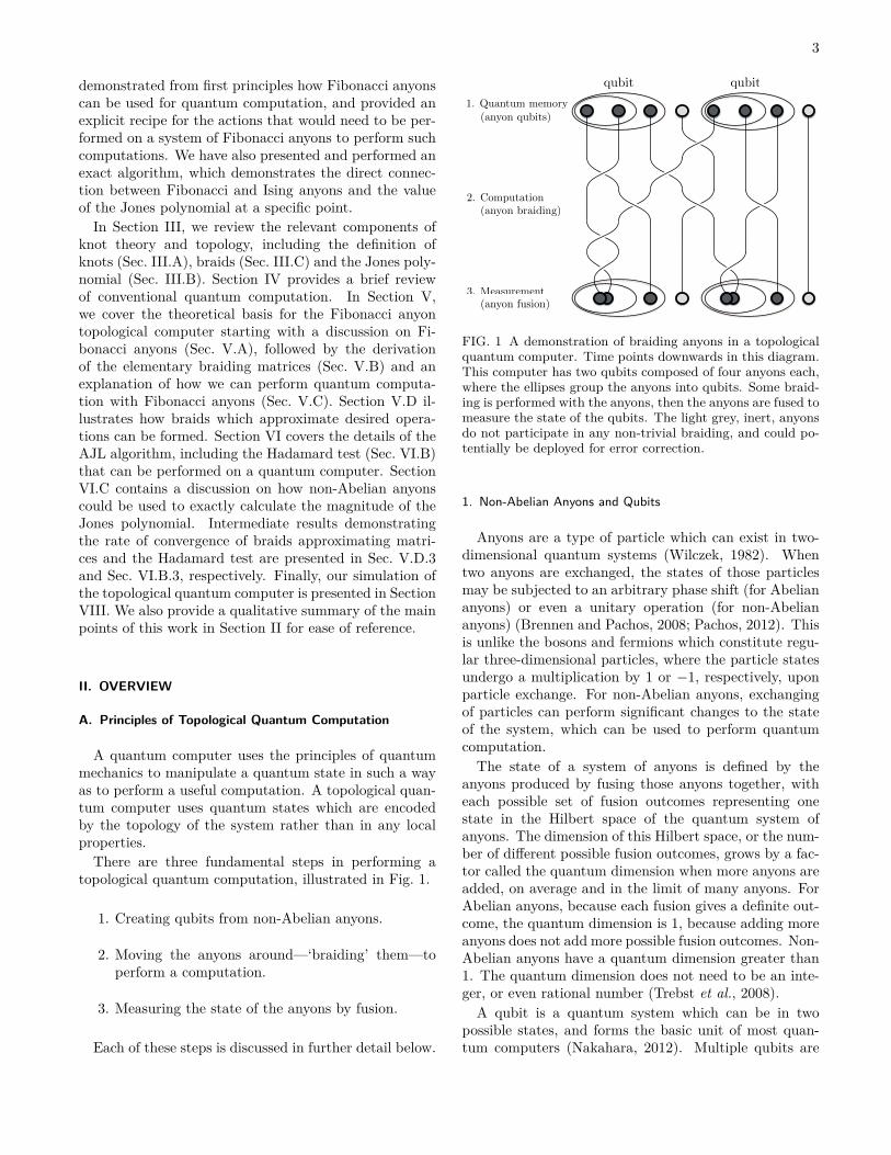
There are three fundamental steps in performing atopological quantum computation, illustrated in Fig. 1.

1. Creating qubits from non-Abelian anyons.

2. Moving the anyons around—‘braiding’ them—toperform a computation.

3. Measuring the state of the anyons by fusion.

Each of these steps is discussed in further detail below.

3. Measurement(anyon fusion)

2. Computation(anyon braiding)

1. Quantum memory(anyon qubits)

qubit qubit

FIG. 1 A demonstration of braiding anyons in a topologicalquantum computer. Time points downwards in this diagram.This computer has two qubits composed of four anyons each,where the ellipses group the anyons into qubits. Some braid-ing is performed with the anyons, then the anyons are fused tomeasure the state of the qubits. The light grey, inert, anyonsdo not participate in any non-trivial braiding, and could po-tentially be deployed for error correction.

1. Non-Abelian Anyons and Qubits

Anyons are a type of particle which can exist in two-dimensional quantum systems (Wilczek, 1982). Whentwo anyons are exchanged, the states of those particlesmay be subjected to an arbitrary phase shift (for Abeliananyons) or even a unitary operation (for non-Abeliananyons) (Brennen and Pachos, 2008; Pachos, 2012). Thisis unlike the bosons and fermions which constitute regu-lar three-dimensional particles, where the particle statesundergo a multiplication by 1 or −1, respectively, uponparticle exchange. For non-Abelian anyons, exchangingof particles can perform significant changes to the stateof the system, which can be used to perform quantumcomputation.The state of a system of anyons is defined by the

anyons produced by fusing those anyons together, witheach possible set of fusion outcomes representing onestate in the Hilbert space of the quantum system ofanyons. The dimension of this Hilbert space, or the num-ber of different possible fusion outcomes, grows by a fac-tor called the quantum dimension when more anyons areadded, on average and in the limit of many anyons. ForAbelian anyons, because each fusion gives a definite out-come, the quantum dimension is 1, because adding moreanyons does not add more possible fusion outcomes. Non-Abelian anyons have a quantum dimension greater than1. The quantum dimension does not need to be an inte-ger, or even rational number (Trebst et al., 2008).A qubit is a quantum system which can be in two

possible states, and forms the basic unit of most quan-tum computers (Nakahara, 2012). Multiple qubits are

4

brought together to form a register of qubits. For topo-logical quantum computers, each qubit is composed of anumber of anyons. In the Fibonacci model, a qubit canbe constructed from four Fibonacci anyons, Fig. 1, withzero net overall ‘charge’ or ‘spin’ (i.e. the four anyonswill annihilate when all of them are fused) (Brennen andPachos, 2008). As such, the first step in performing atopological quantum computation is to create anyons toform a register of qubits.

For the sake of concreteness, we focus on the model ofFibonacci anyons. However, the concepts explored aredirectly applicable to generic non-Abelian anyon models.

2. Braiding Anyons

Exchanging two non-Abelian anyons performs a uni-tary operation on the quantum state, which can changethe relative phases and probability densities of the basisstates corresponding to each fusion outcome.

The anyons exist in two-dimensional space. Considera 2+1 dimensional space, where the third dimensionis time. The worldlines that thread through the timedimension as the anyons move around each other arestrands which are braided, as in Fig. 1. Hence, exchang-ing anyons is referred to as braiding, because the opera-tion braids their worldlines. Furthermore, the operationperformed on the quantum state is dependent solely onthe topology of the braid, meaning that the braid can bestretched and deformed in almost any manner but stillperform the same operation. This topological robustnessprovides the key advantage of topological quantum com-puters over other quantum computers, which is toleranceto errors from local perturbations (Kitaev, 2003; Nayaket al., 2008).

By braiding anyons within a qubit, the probabilities ofthe fusion outcomes within that qubit can be changed.This puts the qubits into a superposition of states. Bybraiding anyons between two qubits, the states of thequbits in general become dependent on each other, suchthat it is not possible to measure the state of one qubitwithout affecting the other qubit. Thus performing abraid which literally entangles two qubits will also inducequantum entanglement between those two qubits.

Before performing any braiding, it is essential to knowwhat braids are necessary to perform the desired opera-tion. In quantum computation, the quantum algorithmsare composed of several quantum gates, which each enacta predetermined operation. It is necessary to determinewhat braid enacts the required gates to within a desiredaccuracy, and this is performed using classical computa-tion with a combination of exhaustive search (Bonesteelet al., 2005) and iterative methods (Burrello et al., 2011;Dawson and Nielsen, 2006; Kitaev, 1997; Kliuchnikovet al., 2014). Once the braid corresponding to a givengate has been determined, that braid can be recorded

for later use during quantum computation. Here we relyon the simpler exhaustive search method, which is ade-quate for first-order approximations of a small number ofquantum gates.

3. Measuring Anyons

After the computation is complete, it is necessary tomeasure the state of the system. This is performed byfusing two of the anyons in each qubit and observing theoutcome of each fusion. Each set of fusion outcomes cor-responds to a unique basis state (Pachos, 2012). Becausethe anyons are a quantum system, the probability of eachset of fusion outcomes is determined by the amplitudesof the basis states in the quantum system.The state of the system after the braiding encodes the

result of the computation. However, the full state can-not be measured directly. As such, it is often necessaryto perform repeated identical computations and measure-ments to statistically determine the probability distribu-tion and thus the state of the system. However, due tothe embarrassing parallelism of such repeated measure-ments, this task can be completed efficiently and simulta-neously by deploying multiple copies of the same system.

4. Physical Realization

A variety of physical systems have been suggested forimplementing topological quantum computation usingnon-Abelian anyons (Nayak et al., 2008; Sarma et al.,2015). Hence, complementing the generic but abstractnotion of anyons, braiding their worldlines, and theireventual fusion as illustrated in Fig. 1, it may be use-ful to have a concrete mental picture of the physical enti-ties and processes comprising such a topological quantumcomputer. For this purpose, we may choose to considerthe anyons to be (quasiparticles associated with) vorticesnucleated in a quasi-two-dimensional superfluid. Suchvortices are the quantum mechanical counterpart to thefamiliar bathtub vortices and are ubiquitous in quantumliquids including superfluid helium-4 (Fonda et al., 2014;Yarmchuk et al., 1979), superfluid helium-3 (Autti et al.,2016; Hakonen et al., 1982), superconductors (Abrikosov,2004; Essmann and Träuble, 1967), Bose–Einstein con-densates (Abo-Shaeer et al., 2001; Fetter, 2009; Madisonet al., 2000; Matthews et al., 1999) and superfluid Fermigases (Zwierlein et al., 2005). The particular types ofnon-Abelian anyons that may be realised depend on thephysical details of the vortices. For example, in chiralp-wave Fermi systems the vortices may host Majoranazero modes (Gurarie and Radzihovsky, 2007; Mizushimaet al., 2008; Volovik, 1999), the topological properties ofwhich correspond to the Majorana zero modes found insolid state systems leading to Ising anyons (Sarma et al.,

5

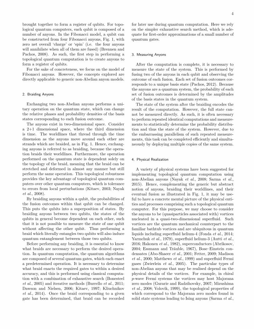
|0i

|ji

HH

�

FIG. 2 Quantum circuit diagram for the Hadamard test forevaluating the real component of a matrix element, as re-quired by the AJL algorithm. The Hadamard gate is denotedby H and the gate Φ is a controlled gate, where the circlemarks the control qubit and the box is the operation actingon the target qubit, with this operation specific to the knotbeing investigated by the AJL algorithm.

2015; Zhang et al., 2018).In a Bose–Einstein condensate, vortex-antivortex pairs

can be spawned from vacuum controllably using e.g.steerable laser beams (Samson et al., 2016). Similar tech-niques could be developed for preparing non-Abelian vor-tex anyons in spinor Bose–Einstein condensates or chiralp-wave Fermi gases to initialise the topological qubits.

Vortices in quantum gases such as Bose-Einstein con-densates can be pinned using focused laser beams (Sam-son et al., 2016; Simula et al., 2008; Tung et al., 2006) andusing optical tweezer technology positions of individualoptical pinning sites can be controllably steered (Robertset al., 2014; Samson et al., 2016) to move vortices aroundadiabatically (Simula, 2018; Virtanen et al., 2001). Whensuch vortices are braided, their worldlines trace out three-dimensional vortex structures familiar from, e.g., studiesof quantum turbulence (Barenghi et al., 2014), propa-gating singular optical fields (Dennis et al., 2010; Taylorand Dennis, 2016; Tempone-Wiltshire et al., 2016), fluidknots (Kleckner and Irvine, 2013), and electron vortices(Petersen et al., 2013).

Fusion of vortices in quantum gases could be achievedby simply overlapping the optical pinning potentials,closing the worldlines such that the vortices will eitherannihilate or form another topological defect. From thetopological quantum computation perspective the mostimportant aspect of such vortices is that they must begoverned by non-Abelian exchange statistics. For thispurpose spinor Bose-Einstein condensates (Kawaguchiand Ueda, 2012; Stamper-Kurn and Ueda, 2013) seemto be a promising platform for searching non-Abelianvortex anyons (Mawson et al., 2018). Many suchhigh-spin Bose-Einstein condensates, including rubidium(Stamper-Kurn and Ueda, 2013), chromium (Griesmaieret al., 2005), erbium (Aikawa et al., 2012), strontium(Stellmer et al., 2009), ytterbium (Takasu et al., 2003)and dysprosium (Lian et al., 2012; Lu et al., 2011)atoms have already been produced. Such spinor Bose-Einstein condensates may host non-Abelian fractional

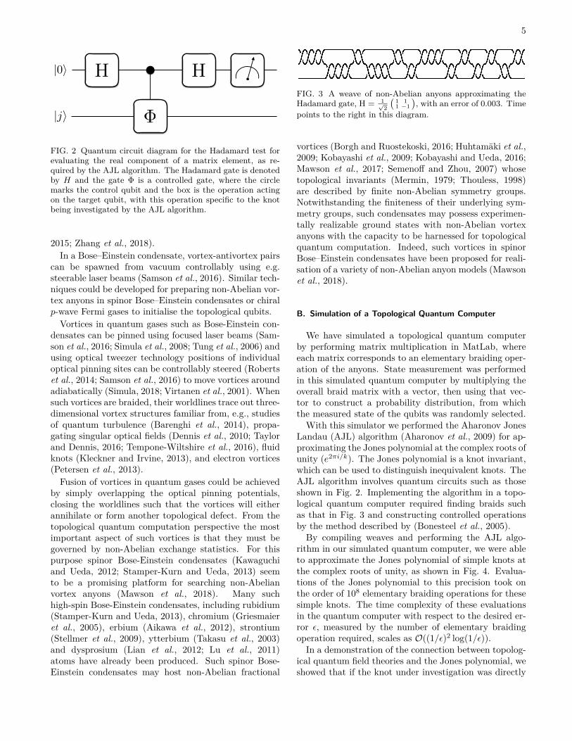
FIG. 3 A weave of non-Abelian anyons approximating theHadamard gate, H = 1√

2

(1 11 −1

), with an error of 0.003. Time

points to the right in this diagram.

vortices (Borgh and Ruostekoski, 2016; Huhtamäki et al.,2009; Kobayashi et al., 2009; Kobayashi and Ueda, 2016;Mawson et al., 2017; Semenoff and Zhou, 2007) whosetopological invariants (Mermin, 1979; Thouless, 1998)are described by finite non-Abelian symmetry groups.Notwithstanding the finiteness of their underlying sym-metry groups, such condensates may possess experimen-tally realizable ground states with non-Abelian vortexanyons with the capacity to be harnessed for topologicalquantum computation. Indeed, such vortices in spinorBose–Einstein condensates have been proposed for reali-sation of a variety of non-Abelian anyon models (Mawsonet al., 2018).

B. Simulation of a Topological Quantum Computer

We have simulated a topological quantum computerby performing matrix multiplication in MatLab, whereeach matrix corresponds to an elementary braiding oper-ation of the anyons. State measurement was performedin this simulated quantum computer by multiplying theoverall braid matrix with a vector, then using that vec-tor to construct a probability distribution, from whichthe measured state of the qubits was randomly selected.With this simulator we performed the Aharonov Jones

Landau (AJL) algorithm (Aharonov et al., 2009) for ap-proximating the Jones polynomial at the complex roots ofunity (e2πi/k). The Jones polynomial is a knot invariant,which can be used to distinguish inequivalent knots. TheAJL algorithm involves quantum circuits such as thoseshown in Fig. 2. Implementing the algorithm in a topo-logical quantum computer required finding braids suchas that in Fig. 3 and constructing controlled operationsby the method described by (Bonesteel et al., 2005).By compiling weaves and performing the AJL algo-

rithm in our simulated quantum computer, we were ableto approximate the Jones polynomial of simple knots atthe complex roots of unity, as shown in Fig. 4. Evalua-tions of the Jones polynomial to this precision took onthe order of 108 elementary braiding operations for thesesimple knots. The time complexity of these evaluationsin the quantum computer with respect to the desired er-ror ε, measured by the number of elementary braidingoperation required, scales as O((1/ε)2 log(1/ε)).

In a demonstration of the connection between topolog-ical quantum field theories and the Jones polynomial, weshowed that if the knot under investigation was directly

6

0.4 0.6 0.8 1 1.2 1.4 1.6-0.4

-0.2

0

0.2

0.4

0.6

0.8

1

1.2

1.4

1.6

Exact value (Re)Exact value (Im)Result (Re)Result (Im)Limiting value (Re)Limiting value (Im)

Vk(t

)

arg(t)

FIG. 4 Results from the determination of the Jones polyno-mial Vk(t) of the positive Hopf link. The horizontal axis showsthe complex phase of the point t where the Jones polynomialis being evaluated. Square markers with error bars are theresults obtained stochastically from the Hadamard test. Realand imaginary components are evaluated separately. The lim-iting values of these stochastic measurements are also shown,see the legend.

copied by the braided worldlines of Fibonacci anyons,then the probability of measuring the initial state is sim-ply the magnitude of the Jones polynomial at the pointt = e2πi/5 times the quantum dimension to a simplepower. An identical result holds for Ising anyons at thepoint t = e2πi/4 = i, and we conjecture that similar re-sults hold for a countably infinite set of anyon models.This method is facile and involves no approximations,but is limited to obtaining the magnitude of the Jonespolynomial at a fixed point. Nevertheless, it facilitatesa straightforward proof of concept demonstration of atopological quantum computer.

We note, however, that the elementary methods usedhere to evaluate the Jones polynomials of knots can beused to simulate any quantum algorithm in a universaltopological quantum computer.

III. TOPOLOGY AND KNOT THEORY

A. Knots

Formally, a knot is a closed loop embedded in three-dimensional space. Intuitively, a knot may be understoodas a tangled loop of string or rope. Knots are studiedwithin the field of topology, meaning that we are permit-ted to stretch, deform and move this loop in a continuousmanner, without cutting the loop or allowing it to inter-sect itself. This type of transformation is referred to asambient isotopy. If two knots are isotopic to one another,

(a) (b) (c)

(d) (e) (f)

FIG. 5 Pictures of (a) the unknot, (b) the Hopf link, (c) thefigure-eight knot, (d) and (e), respectively, the left and righttrefoils, and (f) knot diagram of the right trefoil.

that is, one knot can be deformed into the other, thenthose two knots are equivalent. Otherwise, the knots areinequivalent.Knots can be generalised to being made from multiple

closed loops. Knots containing multiple loops are calledlinks. All the theory which applies to knots can also beapplied to links. In this work we will often use the termsknot and link interchangeably. Knots and links may alsobe oriented, meaning that their curves have an associateddirection.Figure 5 shows pictures of a few simple knots and links.

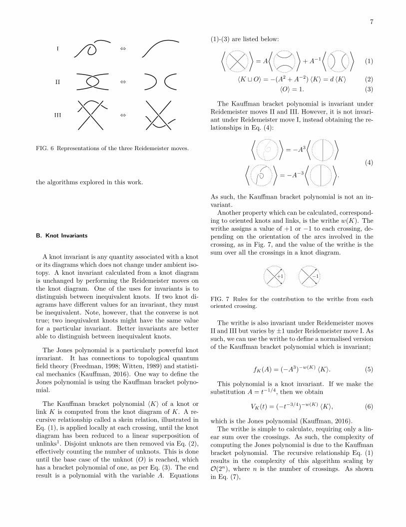
Figure 5(f) is a knot diagram of the knot in Fig. 5(e).Knot diagrams are a projection of knots, which are three-dimensional objects, into a two-dimensional drawing. Ateach intersection on the diagram, the crossing is markedto indicate which arc is above the other in 3D space. TheReidemeister moves, illustrated in Fig. 6, can be usedto manipulate a knot diagram while maintaining ambi-ent isotopy. If one knot diagram can be transformedinto another via a finite number of Reidemeister moves,then those two knots are equivalent (Kauffman, 2016).Not listed is planar isotopy, where the diagram can bestretched and deformed provided no crossings are mod-ified. Planar isotopy is typically assumed to always beallowed.Figure 5(a) shows the simplest possible knot, the un-

knot. It is regarded as a trivial case (although deter-mining whether an arbitrary knot is equivalent to theunknot can be non-trivial). The simplest link is the un-link, which consists of multiple disjoint unknots. It is alsoa trivial case. The simplest non-trivial link is the Hopflink, in Fig. 5(b), and is made of two simple loops, whichintersect each other. The simplest non-trivial knot is thetrefoil, in Fig. 5(d) and Fig. 5(e). The trefoil is chiral,meaning that it is not equivalent to its mirror image. Thenext simplest knot is the figure-eight knot, in Fig. 5(c).These simple knots and links will form the test cases for

7

I ,

II ,

III ,

FIG. 6 Representations of the three Reidemeister moves.

the algorithms explored in this work.

B. Knot Invariants

A knot invariant is any quantity associated with a knotor its diagrams which does not change under ambient iso-topy. A knot invariant calculated from a knot diagramis unchanged by performing the Reidemeister moves onthe knot diagram. One of the uses for invariants is todistinguish between inequivalent knots. If two knot di-agrams have different values for an invariant, they mustbe inequivalent. Note, however, that the converse is nottrue; two inequivalent knots might have the same valuefor a particular invariant. Better invariants are betterable to distinguish between inequivalent knots.

The Jones polynomial is a particularly powerful knotinvariant. It has connections to topological quantumfield theory (Freedman, 1998; Witten, 1989) and statisti-cal mechanics (Kauffman, 2016). One way to define theJones polynomial is using the Kauffman bracket polyno-mial.

The Kauffman bracket polynomial 〈K〉 of a knot orlink K is computed from the knot diagram of K. A re-cursive relationship called a skein relation, illustrated inEq. (1), is applied locally at each crossing, until the knotdiagram has been reduced to a linear superposition ofunlinks1. Disjoint unknots are then removed via Eq. (2),effectively counting the number of unknots. This is doneuntil the base case of the unknot (O) is reached, whichhas a bracket polynomial of one, as per Eq. (3). The endresult is a polynomial with the variable A. Equations

(1)-(3) are listed below:⟨ ⟩= A

⟨ ⟩+A−1

⟨ ⟩(1)

〈K tO〉 = −(A2 +A−2) 〈K〉 = d 〈K〉 (2)〈O〉 = 1. (3)

The Kauffman bracket polynomial is invariant underReidemeister moves II and III. However, it is not invari-ant under Reidemeister move I, instead obtaining the re-lationships in Eq. (4):⟨ ⟩

= −A3

⟨ ⟩⟨ ⟩

= −A−3

⟨ ⟩.

(4)

As such, the Kauffman bracket polynomial is not an in-variant.Another property which can be calculated, correspond-

ing to oriented knots and links, is the writhe w(K). Thewrithe assigns a value of +1 or −1 to each crossing, de-pending on the orientation of the arcs involved in thecrossing, as in Fig. 7, and the value of the writhe is thesum over all the crossings in a knot diagram.

+1 �1

FIG. 7 Rules for the contribution to the writhe from eachoriented crossing.

The writhe is also invariant under Reidemeister movesII and III but varies by ±1 under Reidemeister move I. Assuch, we can use the writhe to define a normalised versionof the Kauffman bracket polynomial which is invariant;

fK(A) = (−A3)−w(K) 〈K〉. (5)

This polynomial is a knot invariant. If we make thesubstitution A = t−1/4, then we obtain

VK(t) = (−t−3/4)−w(K) 〈K〉, (6)

which is the Jones polynomial (Kauffman, 2016).The writhe is simple to calculate, requiring only a lin-

ear sum over the crossings. As such, the complexity ofcomputing the Jones polynomial is due to the Kauffmanbracket polynomial. The recursive relationship Eq. (1)results in the complexity of this algorithm scaling byO(2n), where n is the number of crossings. As shownin Eq. (7),

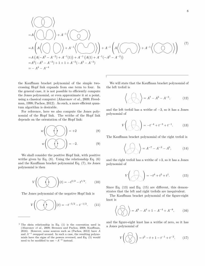
8⟨ ⟩

=A⟨ ⟩

+A−1

⟨ ⟩

=A

A⟨ ⟩+A−1

⟨ ⟩+A−1

A⟨ ⟩+A−1

⟨ ⟩=A

(A(−A2 −A−2) +A−1(1)

)+A−1 (A(1) +A−1(−A2 −A−2)

)=A2(−A2 −A−2) + 1 + 1 +A−2(−A2 −A−2)=−A4 −A−4

(7)

the Kauffman bracket polynomial of the simple two-crossing Hopf link expands from one term to four. Inthe general case, it is not possible to efficiently computethe Jones polynomial, or even approximate it at a point,using a classical computer (Aharonov et al., 2009; Freed-man, 1998; Pachos, 2012). As such, a more efficient quan-tum algorithm is desirable.

For reference, here we also compute the Jones poly-nomial of the Hopf link. The writhe of the Hopf linkdepends on the orientation of the Hopf link:

w

( )= +2 (8)

w

( )= −2. (9)

We shall consider the positive Hopf link, with positivewrithe given by Eq. (8). Using the relationship Eq. (6)and the Kauffman bracket polynomial Eq. (7), its Jonespolynomial is then

V

( )(t) = −t5/2 − t1/2. (10)

The Jones polynomial of the negative Hopf link is

V

( )(t) = −t−5/2 − t−1/2. (11)

1 The skein relationship in Eq. (1) is the convention used in(Aharonov et al., 2009; Brennen and Pachos, 2008; Kauffman,2016). However, some sources such as (Pachos, 2012) have Aand A−1 swapped around. In such a case, the resulting polyno-mials have the signs of the powers reversed, and Eq. (5) wouldneed to be modified to use −A−3 instead.

We will state that the Kauffman bracket polynomial ofthe left trefoil is⟨ ⟩

= A7 −A3 −A−5, (12)

and the left trefoil has a writhe of −3, so it has a Jonespolynomial of

V

( )= −t−4 + t−3 + t−1. (13)

The Kauffman bracket polynomial of the right trefoil is⟨ ⟩= A−7 −A−3 −A5, (14)

and the right trefoil has a writhe of +3, so it has a Jonespolynomial of

V

( )= −t4 + t3 + t1. (15)

Since Eq. (13) and Eq. (15) are different, this demon-strates that the left and right trefoils are inequivalent.The Kauffman bracket polynomial of the figure-eight

knot is⟨ ⟩= A8 −A4 + 1−A−4 +A−8, (16)

and the figure-eight knot has a writhe of zero, so it hasa Jones polynomial of

V

( )= t2 − t+ 1− t−1 + t−2. (17)

9

=

=

=

b1 b2 b3 (b1)�1

b1b2b1 = b2b1b2

b3b1 = b1b3

b1(b1)�1 = 1

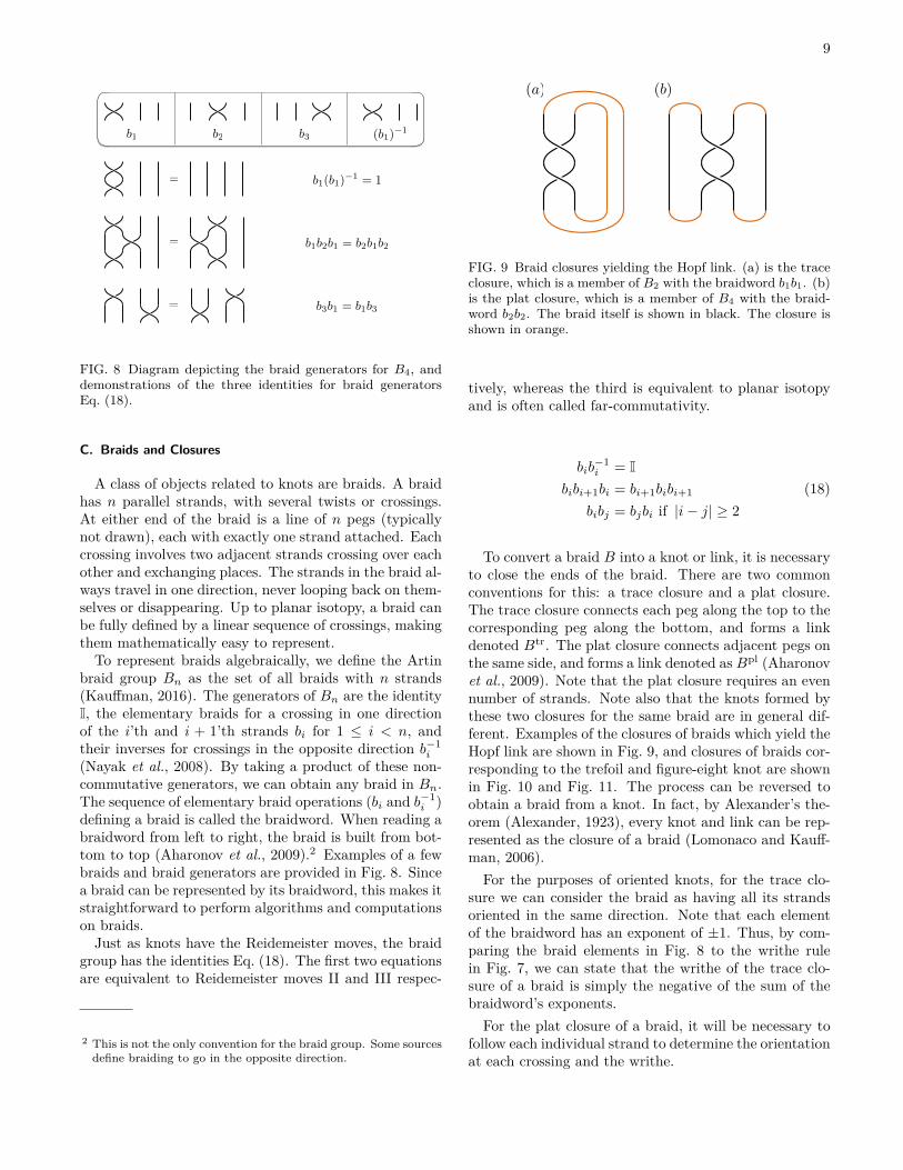
FIG. 8 Diagram depicting the braid generators for B4, anddemonstrations of the three identities for braid generatorsEq. (18).

C. Braids and Closures

A class of objects related to knots are braids. A braidhas n parallel strands, with several twists or crossings.At either end of the braid is a line of n pegs (typicallynot drawn), each with exactly one strand attached. Eachcrossing involves two adjacent strands crossing over eachother and exchanging places. The strands in the braid al-ways travel in one direction, never looping back on them-selves or disappearing. Up to planar isotopy, a braid canbe fully defined by a linear sequence of crossings, makingthem mathematically easy to represent.

To represent braids algebraically, we define the Artinbraid group Bn as the set of all braids with n strands(Kauffman, 2016). The generators of Bn are the identityI, the elementary braids for a crossing in one directionof the i’th and i + 1’th strands bi for 1 ≤ i < n, andtheir inverses for crossings in the opposite direction b−1

i

(Nayak et al., 2008). By taking a product of these non-commutative generators, we can obtain any braid in Bn.The sequence of elementary braid operations (bi and b−1

i )defining a braid is called the braidword. When reading abraidword from left to right, the braid is built from bot-tom to top (Aharonov et al., 2009).2 Examples of a fewbraids and braid generators are provided in Fig. 8. Sincea braid can be represented by its braidword, this makes itstraightforward to perform algorithms and computationson braids.

Just as knots have the Reidemeister moves, the braidgroup has the identities Eq. (18). The first two equationsare equivalent to Reidemeister moves II and III respec-

2 This is not the only convention for the braid group. Some sourcesdefine braiding to go in the opposite direction.

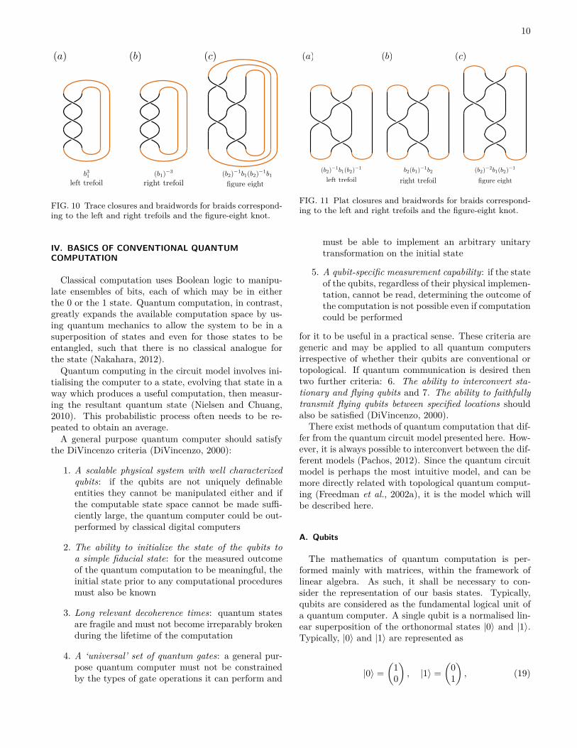
(a) (b)

FIG. 9 Braid closures yielding the Hopf link. (a) is the traceclosure, which is a member of B2 with the braidword b1b1. (b)is the plat closure, which is a member of B4 with the braid-word b2b2. The braid itself is shown in black. The closure isshown in orange.

tively, whereas the third is equivalent to planar isotopyand is often called far-commutativity.

bib−1i = I

bibi+1bi = bi+1bibi+1

bibj = bjbi if |i− j| ≥ 2(18)

To convert a braid B into a knot or link, it is necessaryto close the ends of the braid. There are two commonconventions for this: a trace closure and a plat closure.The trace closure connects each peg along the top to thecorresponding peg along the bottom, and forms a linkdenoted Btr. The plat closure connects adjacent pegs onthe same side, and forms a link denoted as Bpl (Aharonovet al., 2009). Note that the plat closure requires an evennumber of strands. Note also that the knots formed bythese two closures for the same braid are in general dif-ferent. Examples of the closures of braids which yield theHopf link are shown in Fig. 9, and closures of braids cor-responding to the trefoil and figure-eight knot are shownin Fig. 10 and Fig. 11. The process can be reversed toobtain a braid from a knot. In fact, by Alexander’s the-orem (Alexander, 1923), every knot and link can be rep-resented as the closure of a braid (Lomonaco and Kauff-man, 2006).For the purposes of oriented knots, for the trace clo-

sure we can consider the braid as having all its strandsoriented in the same direction. Note that each elementof the braidword has an exponent of ±1. Thus, by com-paring the braid elements in Fig. 8 to the writhe rulein Fig. 7, we can state that the writhe of the trace clo-sure of a braid is simply the negative of the sum of thebraidword’s exponents.For the plat closure of a braid, it will be necessary to

follow each individual strand to determine the orientationat each crossing and the writhe.

10

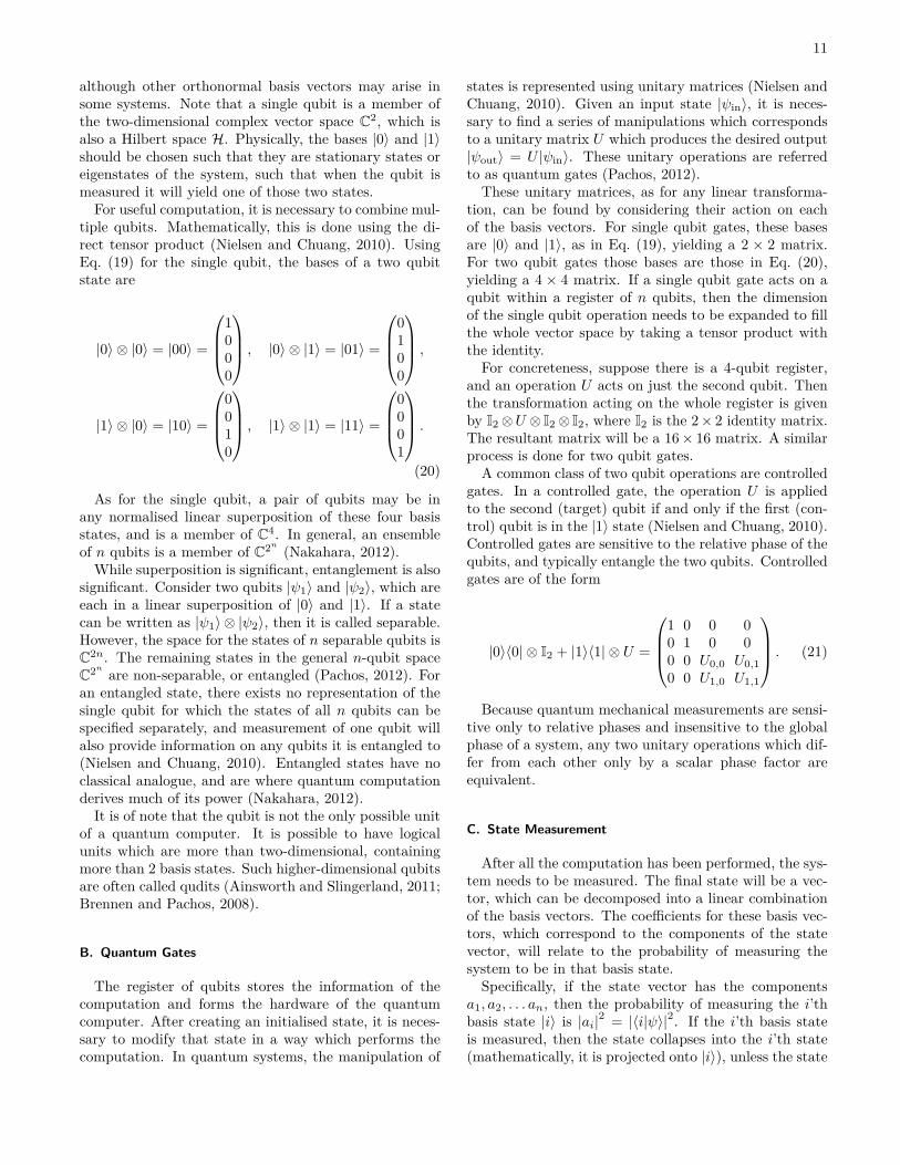
(a) (b) (c)

left trefoil right trefoil figure eight

(b2)�1b1(b2)

�1b1(b1)�3b3

1

FIG. 10 Trace closures and braidwords for braids correspond-ing to the left and right trefoils and the figure-eight knot.

IV. BASICS OF CONVENTIONAL QUANTUMCOMPUTATION

Classical computation uses Boolean logic to manipu-late ensembles of bits, each of which may be in eitherthe 0 or the 1 state. Quantum computation, in contrast,greatly expands the available computation space by us-ing quantum mechanics to allow the system to be in asuperposition of states and even for those states to beentangled, such that there is no classical analogue forthe state (Nakahara, 2012).

Quantum computing in the circuit model involves ini-tialising the computer to a state, evolving that state in away which produces a useful computation, then measur-ing the resultant quantum state (Nielsen and Chuang,2010). This probabilistic process often needs to be re-peated to obtain an average.

A general purpose quantum computer should satisfythe DiVincenzo criteria (DiVincenzo, 2000):

1. A scalable physical system with well characterizedqubits: if the qubits are not uniquely definableentities they cannot be manipulated either and ifthe computable state space cannot be made suffi-ciently large, the quantum computer could be out-performed by classical digital computers

2. The ability to initialize the state of the qubits toa simple fiducial state: for the measured outcomeof the quantum computation to be meaningful, theinitial state prior to any computational proceduresmust also be known

3. Long relevant decoherence times: quantum statesare fragile and must not become irreparably brokenduring the lifetime of the computation

4. A ‘universal’ set of quantum gates: a general pur-pose quantum computer must not be constrainedby the types of gate operations it can perform and

(a) (b) (c)

left trefoil right trefoil figure eight

(b2)�1b1(b2)

�1 b2(b1)�1b2 (b2)

�2b1(b2)�1

FIG. 11 Plat closures and braidwords for braids correspond-ing to the left and right trefoils and the figure-eight knot.

must be able to implement an arbitrary unitarytransformation on the initial state

5. A qubit-specific measurement capability: if the stateof the qubits, regardless of their physical implemen-tation, cannot be read, determining the outcome ofthe computation is not possible even if computationcould be performed

for it to be useful in a practical sense. These criteria aregeneric and may be applied to all quantum computersirrespective of whether their qubits are conventional ortopological. If quantum communication is desired thentwo further criteria: 6. The ability to interconvert sta-tionary and flying qubits and 7. The ability to faithfullytransmit flying qubits between specified locations shouldalso be satisfied (DiVincenzo, 2000).There exist methods of quantum computation that dif-

fer from the quantum circuit model presented here. How-ever, it is always possible to interconvert between the dif-ferent models (Pachos, 2012). Since the quantum circuitmodel is perhaps the most intuitive model, and can bemore directly related with topological quantum comput-ing (Freedman et al., 2002a), it is the model which willbe described here.

A. Qubits

The mathematics of quantum computation is per-formed mainly with matrices, within the framework oflinear algebra. As such, it shall be necessary to con-sider the representation of our basis states. Typically,qubits are considered as the fundamental logical unit ofa quantum computer. A single qubit is a normalised lin-ear superposition of the orthonormal states |0〉 and |1〉.Typically, |0〉 and |1〉 are represented as

|0〉 =(

10

), |1〉 =

(01

), (19)

11

although other orthonormal basis vectors may arise insome systems. Note that a single qubit is a member ofthe two-dimensional complex vector space C2, which isalso a Hilbert space H. Physically, the bases |0〉 and |1〉should be chosen such that they are stationary states oreigenstates of the system, such that when the qubit ismeasured it will yield one of those two states.

For useful computation, it is necessary to combine mul-tiple qubits. Mathematically, this is done using the di-rect tensor product (Nielsen and Chuang, 2010). UsingEq. (19) for the single qubit, the bases of a two qubitstate are

|0〉 ⊗ |0〉 = |00〉 =

1000

, |0〉 ⊗ |1〉 = |01〉 =

0100

,

|1〉 ⊗ |0〉 = |10〉 =

0010

, |1〉 ⊗ |1〉 = |11〉 =

0001

.

(20)

As for the single qubit, a pair of qubits may be inany normalised linear superposition of these four basisstates, and is a member of C4. In general, an ensembleof n qubits is a member of C2n (Nakahara, 2012).While superposition is significant, entanglement is also

significant. Consider two qubits |ψ1〉 and |ψ2〉, which areeach in a linear superposition of |0〉 and |1〉. If a statecan be written as |ψ1〉 ⊗ |ψ2〉, then it is called separable.However, the space for the states of n separable qubits isC2n. The remaining states in the general n-qubit spaceC2n are non-separable, or entangled (Pachos, 2012). Foran entangled state, there exists no representation of thesingle qubit for which the states of all n qubits can bespecified separately, and measurement of one qubit willalso provide information on any qubits it is entangled to(Nielsen and Chuang, 2010). Entangled states have noclassical analogue, and are where quantum computationderives much of its power (Nakahara, 2012).

It is of note that the qubit is not the only possible unitof a quantum computer. It is possible to have logicalunits which are more than two-dimensional, containingmore than 2 basis states. Such higher-dimensional qubitsare often called qudits (Ainsworth and Slingerland, 2011;Brennen and Pachos, 2008).

B. Quantum Gates

The register of qubits stores the information of thecomputation and forms the hardware of the quantumcomputer. After creating an initialised state, it is neces-sary to modify that state in a way which performs thecomputation. In quantum systems, the manipulation of

states is represented using unitary matrices (Nielsen andChuang, 2010). Given an input state |ψin〉, it is neces-sary to find a series of manipulations which correspondsto a unitary matrix U which produces the desired output|ψout〉 = U |ψin〉. These unitary operations are referredto as quantum gates (Pachos, 2012).These unitary matrices, as for any linear transforma-

tion, can be found by considering their action on eachof the basis vectors. For single qubit gates, these basesare |0〉 and |1〉, as in Eq. (19), yielding a 2 × 2 matrix.For two qubit gates those bases are those in Eq. (20),yielding a 4 × 4 matrix. If a single qubit gate acts on aqubit within a register of n qubits, then the dimensionof the single qubit operation needs to be expanded to fillthe whole vector space by taking a tensor product withthe identity.For concreteness, suppose there is a 4-qubit register,

and an operation U acts on just the second qubit. Thenthe transformation acting on the whole register is givenby I2⊗U ⊗ I2⊗ I2, where I2 is the 2× 2 identity matrix.The resultant matrix will be a 16× 16 matrix. A similarprocess is done for two qubit gates.A common class of two qubit operations are controlled

gates. In a controlled gate, the operation U is appliedto the second (target) qubit if and only if the first (con-trol) qubit is in the |1〉 state (Nielsen and Chuang, 2010).Controlled gates are sensitive to the relative phase of thequbits, and typically entangle the two qubits. Controlledgates are of the form

|0〉〈0| ⊗ I2 + |1〉〈1| ⊗ U =

1 0 0 00 1 0 00 0 U0,0 U0,10 0 U1,0 U1,1

. (21)

Because quantum mechanical measurements are sensi-tive only to relative phases and insensitive to the globalphase of a system, any two unitary operations which dif-fer from each other only by a scalar phase factor areequivalent.

C. State Measurement

After all the computation has been performed, the sys-tem needs to be measured. The final state will be a vec-tor, which can be decomposed into a linear combinationof the basis vectors. The coefficients for these basis vec-tors, which correspond to the components of the statevector, will relate to the probability of measuring thesystem to be in that basis state.Specifically, if the state vector has the components

a1, a2, . . . an, then the probability of measuring the i’thbasis state |i〉 is |ai|2 = |〈i|ψ〉|2. If the i’th basis stateis measured, then the state collapses into the i’th state(mathematically, it is projected onto |i〉), unless the state

12

|0i

|0i NOT

NOT

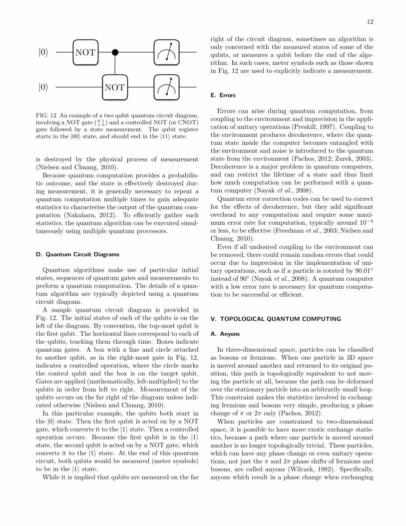
FIG. 12 An example of a two qubit quantum circuit diagram,involving a NOT gate ( 0 1

1 0 ) and a controlled NOT (or CNOT)gate followed by a state measurement. The qubit registerstarts in the |00〉 state, and should end in the |11〉 state.

is destroyed by the physical process of measurement(Nielsen and Chuang, 2010).

Because quantum computation provides a probabilis-tic outcome, and the state is effectively destroyed dur-ing measurement, it is generally necessary to repeat aquantum computation multiple times to gain adequatestatistics to characterise the output of the quantum com-putation (Nakahara, 2012). To efficiently gather suchstatistics, the quantum algorithm can be executed simul-taneously using multiple quantum processors.

D. Quantum Circuit Diagrams

Quantum algorithms make use of particular initialstates, sequences of quantum gates and measurements toperform a quantum computation. The details of a quan-tum algorithm are typically depicted using a quantumcircuit diagram.

A sample quantum circuit diagram is provided inFig. 12. The initial states of each of the qubits is on theleft of the diagram. By convention, the top-most qubit isthe first qubit. The horizontal lines correspond to each ofthe qubits, tracking them through time. Boxes indicatequantum gates. A box with a line and circle attachedto another qubit, as in the right-most gate in Fig. 12,indicates a controlled operation, where the circle marksthe control qubit and the box is on the target qubit.Gates are applied (mathematically, left-multiplied) to thequbits in order from left to right. Measurement of thequbits occurs on the far right of the diagram unless indi-cated otherwise (Nielsen and Chuang, 2010).

In this particular example, the qubits both start inthe |0〉 state. Then the first qubit is acted on by a NOTgate, which converts it to the |1〉 state. Then a controlledoperation occurs. Because the first qubit is in the |1〉state, the second qubit is acted on by a NOT gate, whichconverts it to the |1〉 state. At the end of this quantumcircuit, both qubits would be measured (meter symbols)to be in the |1〉 state.

While it is implied that qubits are measured on the far

right of the circuit diagram, sometimes an algorithm isonly concerned with the measured states of some of thequbits, or measures a qubit before the end of the algo-rithm. In such cases, meter symbols such as those shownin Fig. 12 are used to explicitly indicate a measurement.

E. Errors

Errors can arise during quantum computation, fromcoupling to the environment and imprecision in the appli-cation of unitary operations (Preskill, 1997). Coupling tothe environment produces decoherence, where the quan-tum state inside the computer becomes entangled withthe environment and noise is introduced to the quantumstate from the environment (Pachos, 2012; Zurek, 2003).Decoherence is a major problem in quantum computers,and can restrict the lifetime of a state and thus limithow much computation can be performed with a quan-tum computer (Nayak et al., 2008).Quantum error correction codes can be used to correct

for the effects of decoherence, but they add significantoverhead to any computation and require some maxi-mum error rate for computation, typically around 10−4

or less, to be effective (Freedman et al., 2003; Nielsen andChuang, 2010).Even if all undesired coupling to the environment can

be removed, there could remain random errors that couldoccur due to imprecision in the implementation of uni-tary operations, such as if a particle is rotated by 90.01◦instead of 90◦ (Nayak et al., 2008). A quantum computerwith a low error rate is necessary for quantum computa-tion to be successful or efficient.

V. TOPOLOGICAL QUANTUM COMPUTING

A. Anyons

In three-dimensional space, particles can be classifiedas bosons or fermions. When one particle in 3D spaceis moved around another and returned to its original po-sition, this path is topologically equivalent to not mov-ing the particle at all, because the path can be deformedover the stationary particle into an arbitrarily small loop.This constraint makes the statistics involved in exchang-ing fermions and bosons very simple, producing a phasechange of π or 2π only (Pachos, 2012).When particles are constrained to two-dimensional

space, it is possible to have more exotic exchange statis-tics, because a path where one particle is moved aroundanother is no longer topologically trivial. These particles,which can have any phase change or even unitary opera-tions, not just the π and 2π phase shifts of fermions andbosons, are called anyons (Wilczek, 1982). Specifically,anyons which result in a phase change when exchanging

13

the positions of two particles are classified as Abeliananyons, because the operations produced by exchangingthe anyons all commute with each other. However, it ispossible for exchanging anyons to result in unitary oper-ations beyond simple phase changes, and such particlesare classified as non-Abelian anyons, because the opera-tions produced by exchanging the anyons in general donot commute (Brennen and Pachos, 2008; Burton, 2016;Nayak et al., 2008; Preskill, 2004; Stern, 2008; Trebstet al., 2008). It is non-Abelian anyons which are of in-terest to quantum computation.

The state of a system of anyons is defined by the anyonsproduced by fusing those anyons together, with each pos-sible set of fusion outcomes representing one basis state inthe Hilbert space of the quantum system of anyons. Eachmodel of anyons contains rules regarding the possible out-comes of the fusion of two anyons. Abelian anyons haveonly a single possible fusion outcome for each fusion pair.When two non-Abelian anyons are fused, however, thereare multiple possible fusion outcomes (Preskill, 2004).

Adding more anyons to the system typically increasesthe number of possible states, and the factor by whichthis number increases is the quantum dimension. Whenan Abelian anyon is fused with another anyon, there isonly one possible outcome, so Abelian anyons have aquantum dimension of 1. When two non-Abelian anyonsare fused, then there are multiple possible outcomes, de-termined probabilistically, so non-Abelian anyons have aquantum dimension greater than 1 (Nayak et al., 2008;Pachos, 2012; Trebst et al., 2008).

The simplest model of non-Abelian anyons is the Fi-bonacci model. A Fibonacci anyon may fuse with an-other Fibonacci anyon to either annihilate or to produceanother Fibonacci anyon. The number of possible fusionoutcomes grows by the Fibonacci sequence when moreanyons are added (hence the name), giving Fibonaccianyons a quantum dimension of the golden ratio, 1+

√5

2(Nayak et al., 2008). Furthermore, it has been demon-strated that the operations performed by exchanging Fi-bonacci anyons can reproduce any unitary operation toarbitrary accuracy (up to a global phase factor) (Freed-man et al., 2002b), which makes Fibonacci anyons uni-versal for quantum computation.

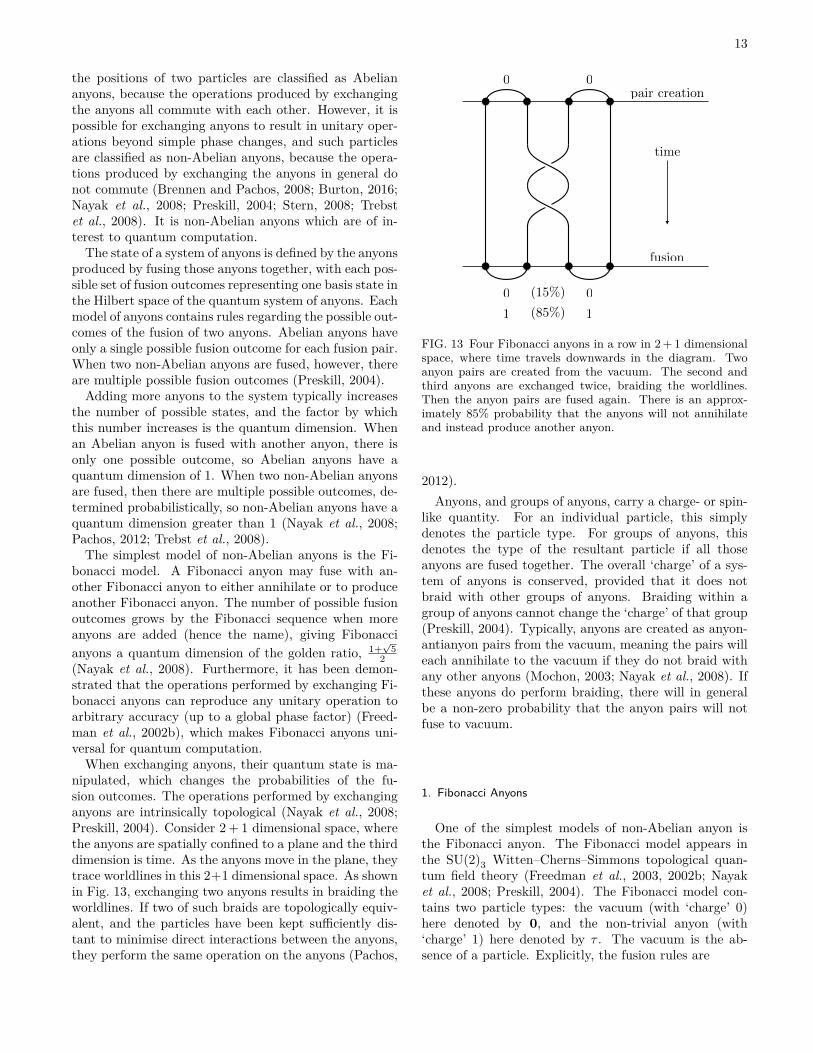
When exchanging anyons, their quantum state is ma-nipulated, which changes the probabilities of the fu-sion outcomes. The operations performed by exchanginganyons are intrinsically topological (Nayak et al., 2008;Preskill, 2004). Consider 2 + 1 dimensional space, wherethe anyons are spatially confined to a plane and the thirddimension is time. As the anyons move in the plane, theytrace worldlines in this 2+1 dimensional space. As shownin Fig. 13, exchanging two anyons results in braiding theworldlines. If two of such braids are topologically equiv-alent, and the particles have been kept sufficiently dis-tant to minimise direct interactions between the anyons,they perform the same operation on the anyons (Pachos,

0 0

1

(15%)

(85%)

0 0

1

time

pair creation

fusion

FIG. 13 Four Fibonacci anyons in a row in 2 + 1 dimensionalspace, where time travels downwards in the diagram. Twoanyon pairs are created from the vacuum. The second andthird anyons are exchanged twice, braiding the worldlines.Then the anyon pairs are fused again. There is an approx-imately 85% probability that the anyons will not annihilateand instead produce another anyon.

2012).Anyons, and groups of anyons, carry a charge- or spin-

like quantity. For an individual particle, this simplydenotes the particle type. For groups of anyons, thisdenotes the type of the resultant particle if all thoseanyons are fused together. The overall ‘charge’ of a sys-tem of anyons is conserved, provided that it does notbraid with other groups of anyons. Braiding within agroup of anyons cannot change the ‘charge’ of that group(Preskill, 2004). Typically, anyons are created as anyon-antianyon pairs from the vacuum, meaning the pairs willeach annihilate to the vacuum if they do not braid withany other anyons (Mochon, 2003; Nayak et al., 2008). Ifthese anyons do perform braiding, there will in generalbe a non-zero probability that the anyon pairs will notfuse to vacuum.

1. Fibonacci Anyons

One of the simplest models of non-Abelian anyon isthe Fibonacci anyon. The Fibonacci model appears inthe SU(2)3 Witten–Cherns–Simmons topological quan-tum field theory (Freedman et al., 2003, 2002b; Nayaket al., 2008; Preskill, 2004). The Fibonacci model con-tains two particle types: the vacuum (with ‘charge’ 0)here denoted by 0, and the non-trivial anyon (with‘charge’ 1) here denoted by τ . The vacuum is the ab-sence of a particle. Explicitly, the fusion rules are

14

τ ⊗ τ = 0⊕ τ0⊗ 0 = 00⊗ τ = τ

τ ⊗ 0 = τ,

(22)

where ⊗ in this context denotes the fusion (merging) oftwo particles and ⊕ denotes multiple possible outcomes.In the following, we refer to the anyons 0 and τ of theFibonacci model simply by their charges 0 and 1, respec-tively. Fusion of two Fibonacci anyons may result in ei-ther annihilation or creation of a new anyon. This makesthe Fibonacci anyon its own anti-particle (Pachos, 2012;Preskill, 2004). From the last three rules, fusion withthe vacuum does nothing. As is shown later, performingbraiding can change the probabilities of the outcomes ofthis fusion.

Consider Fig. 13. Since the pairs are created from thevacuum, each pair must have a net ‘charge’ of 0. If thebraid was not present, then the two pairs would individu-ally fuse to vacuum with 100% probability. However, byperforming the braiding then fusing the particles, thereis a non-zero probability that the fusion could give 1 in-stead of 0. The net ‘charge’ of the whole system is still 0,though, so if the remaining two particles are fused, theymust give the vacuum. From Eq. (22) this is only pos-sible if either both particles are 0 or both particles are1. This means that, for this system, the outcome of thefusion of one of the pairs of anyons determines the fusionoutcome of the other pair.

For Fibonacci anyons, the number of possible fu-sion outcomes, and thus the dimension of the Hilbertspace, grows according to the Fibonacci sequence as moreanyons are added. This gives Fibonacci anyons a quan-tum dimension dτ of the golden ratio, dτ = φ = 1+

√5

2 ,and is where Fibonacci anyons get their name (Pachos,2012; Preskill, 2004). Generically, the quantum dimen-sions of the anyons satisfy dαdβ =

∑γ N

γαβdγ , where the

integer Nγαβ is the number of distinguishable ways the

anyons α and β may be fused to yield an anyon γ. Thetotal quantum dimension D of the anyon model is deter-mined by the relation D =

√∑α d

2α (Nayak et al., 2008;

Preskill, 2004). Abelian anyons have a quantum dimen-sion equal to one, where as for non-Abelian anyons theirquantum dimension is greater than one. Non-Abeliananyons, such as Fibonacci anyons, are thought to becapable of universal quantum computation by braidingalone if the square of their quantum dimension is not in-teger. The quantum dimension has also been linked tothe passage of time by showing that a relational timefor universal anyonic systems, such as the Fibonaccianyon model, is continuous where as for non-universalsystems, such as the Ising anyon model, discrete timewould emerge (Nikolova et al., 2018).There are several candidate systems which may exhibit

the behaviours of Fibonacci anyons (Alicea and Stern,2015; Sarma et al., 2015). One candidate is the fractionalHall effect at v = 12/5, which can exhibit quasiparticleexcitations which are predicted to follow the behaviourof Fibonacci anyons (Ardonne and Schoutens, 2007; Bon-derson et al., 2006; Brennen and Pachos, 2008; Monget al., 2017; Nayak et al., 2008; Rezayi and Read, 2009;Sarma et al., 2006; Stern, 2008; Trebst et al., 2008; Wuet al., 2014). Another candidate is to construct networksof spin lattices which mimic the desired anyon behaviours(Brennen and Pachos, 2008). Other candidates such asrotating Bose-Einstein condensates (Cooper et al., 2001),dipolar boson lattices (Ðurić et al., 2017) and magneticsystems (Fendley et al., 2013) have also been proposed.This work does not concern itself with any specific

physical model of Fibonacci anyon and instead focuses onthe macroscopic properties of the Fibonacci anyons withregards to braiding and fusion outcomes. In ignoringmore specific physical implementations, we assume thatit is possible to reliably create anyon pairs, move thoseanyons around each other, and determine the outcome ofanyon fusion. In general, these tasks may be non-trivialin a physical system, but such challenges are beyond thescope of this work. Notwithstanding, the reader maychoose to refer to the non-Abelian vortex anyon modelsmentioned in Sec. II.

B. Braiding

1. The F Move

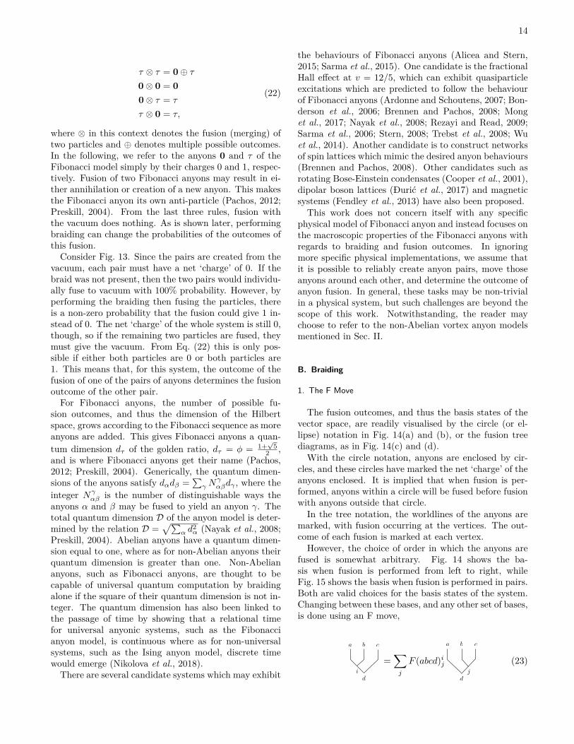
The fusion outcomes, and thus the basis states of thevector space, are readily visualised by the circle (or el-lipse) notation in Fig. 14(a) and (b), or the fusion treediagrams, as in Fig. 14(c) and (d).With the circle notation, anyons are enclosed by cir-

cles, and these circles have marked the net ‘charge’ of theanyons enclosed. It is implied that when fusion is per-formed, anyons within a circle will be fused before fusionwith anyons outside that circle.In the tree notation, the worldlines of the anyons are

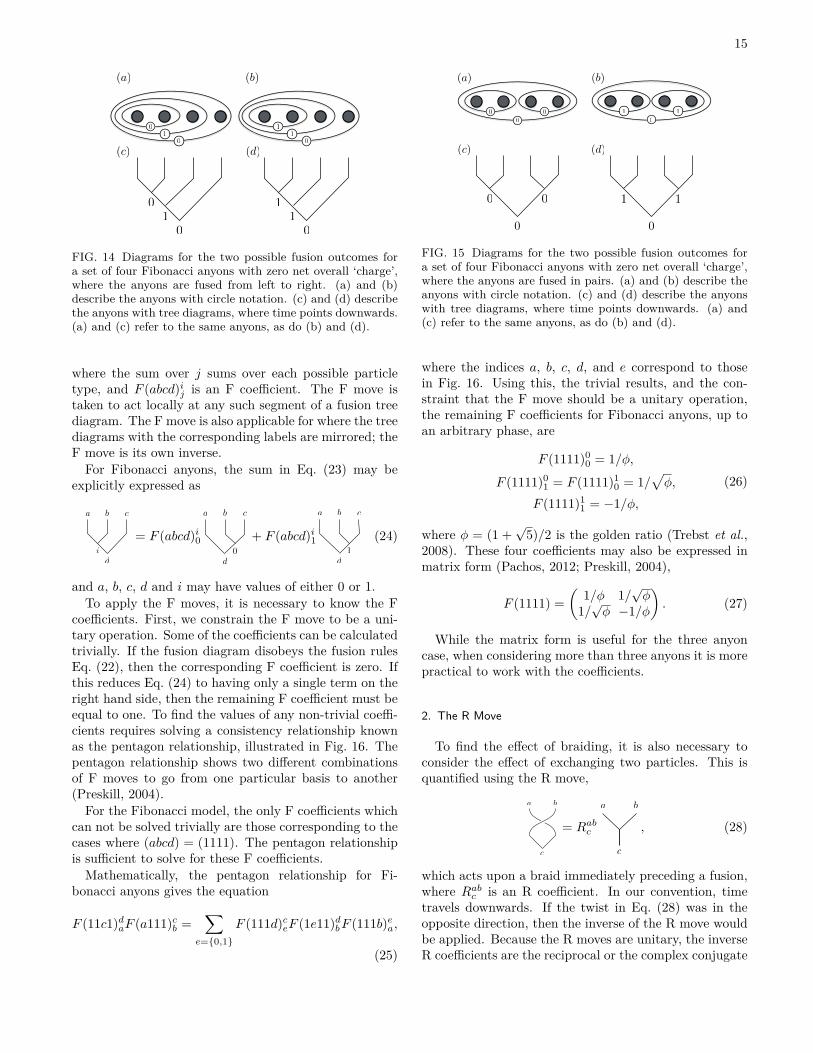
marked, with fusion occurring at the vertices. The out-come of each fusion is marked at each vertex.However, the choice of order in which the anyons are

fused is somewhat arbitrary. Fig. 14 shows the ba-sis when fusion is performed from left to right, whileFig. 15 shows the basis when fusion is performed in pairs.Both are valid choices for the basis states of the system.Changing between these bases, and any other set of bases,is done using an F move,

a b c

di

=∑j

F (abcd)ij

a b c

dj

(23)

15

(a) (b)

10

0

11

0

(c) (d)

10

01

0

1

FIG. 14 Diagrams for the two possible fusion outcomes fora set of four Fibonacci anyons with zero net overall ‘charge’,where the anyons are fused from left to right. (a) and (b)describe the anyons with circle notation. (c) and (d) describethe anyons with tree diagrams, where time points downwards.(a) and (c) refer to the same anyons, as do (b) and (d).

where the sum over j sums over each possible particletype, and F (abcd)ij is an F coefficient. The F move istaken to act locally at any such segment of a fusion treediagram. The F move is also applicable for where the treediagrams with the corresponding labels are mirrored; theF move is its own inverse.

For Fibonacci anyons, the sum in Eq. (23) may beexplicitly expressed as

a b c

di

= F (abcd)i0

a b c

d0

+ F (abcd)i1

a b c

d1

(24)

and a, b, c, d and i may have values of either 0 or 1.To apply the F moves, it is necessary to know the F

coefficients. First, we constrain the F move to be a uni-tary operation. Some of the coefficients can be calculatedtrivially. If the fusion diagram disobeys the fusion rulesEq. (22), then the corresponding F coefficient is zero. Ifthis reduces Eq. (24) to having only a single term on theright hand side, then the remaining F coefficient must beequal to one. To find the values of any non-trivial coeffi-cients requires solving a consistency relationship knownas the pentagon relationship, illustrated in Fig. 16. Thepentagon relationship shows two different combinationsof F moves to go from one particular basis to another(Preskill, 2004).

For the Fibonacci model, the only F coefficients whichcan not be solved trivially are those corresponding to thecases where (abcd) = (1111). The pentagon relationshipis sufficient to solve for these F coefficients.

Mathematically, the pentagon relationship for Fi-bonacci anyons gives the equation

F (11c1)daF (a111)cb =∑

e={0,1}F (111d)ceF (1e11)dbF (111b)ea,

(25)

0

0

0 11

0

00

00

11

(a)

(c)

(b)

(d)

FIG. 15 Diagrams for the two possible fusion outcomes fora set of four Fibonacci anyons with zero net overall ‘charge’,where the anyons are fused in pairs. (a) and (b) describe theanyons with circle notation. (c) and (d) describe the anyonswith tree diagrams, where time points downwards. (a) and(c) refer to the same anyons, as do (b) and (d).

where the indices a, b, c, d, and e correspond to thosein Fig. 16. Using this, the trivial results, and the con-straint that the F move should be a unitary operation,the remaining F coefficients for Fibonacci anyons, up toan arbitrary phase, are

F (1111)00 = 1/φ,

F (1111)01 = F (1111)1

0 = 1/√φ,

F (1111)11 = −1/φ,

(26)

where φ = (1 +√

5)/2 is the golden ratio (Trebst et al.,2008). These four coefficients may also be expressed inmatrix form (Pachos, 2012; Preskill, 2004),

F (1111) =(

1/φ 1/√φ

1/√φ −1/φ

). (27)

While the matrix form is useful for the three anyoncase, when considering more than three anyons it is morepractical to work with the coefficients.

2. The R Move

To find the effect of braiding, it is also necessary toconsider the effect of exchanging two particles. This isquantified using the R move,

a b

c

= Rabc

a b

c

, (28)

which acts upon a braid immediately preceding a fusion,where Rabc is an R coefficient. In our convention, timetravels downwards. If the twist in Eq. (28) was in theopposite direction, then the inverse of the R move wouldbe applied. Because the R moves are unitary, the inverseR coefficients are the reciprocal or the complex conjugate

16

)))

))

F

F F

F F

ab d

e

ca

c

de

b

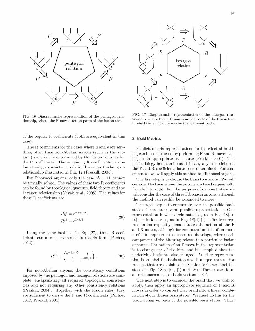
pentagonrelation

FIG. 16 Diagrammatic representation of the pentagon rela-tionship, where the F moves act on parts of the fusion tree.

of the regular R coefficients (both are equivalent in thiscase).

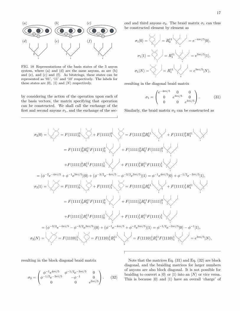
The R coefficients for the cases where a and b are any-thing other than non-Abelian anyons (such as the vac-uum) are trivially determined by the fusion rules, as forthe F coefficients. The remaining R coefficients can befound using a consistency relation known as the hexagonrelationship illustrated in Fig. 17 (Preskill, 2004).

For Fibonacci anyons, only the case ab = 11 cannotbe trivially solved. The values of these two R coefficientscan be found by topological quantum field theory and thehexagon relationship (Nayak et al., 2008). The values forthese R coefficients are

R110 = e−4πi/5,

R111 = e3πi/5.

(29)

Using the same basis as for Eq. (27), these R coef-ficients can also be expressed in matrix form (Pachos,2012),

R11 =(e−4πi/5 0

0 e3πi/5

). (30)

For non-Abelian anyons, the consistency conditionsimposed by the pentagon and hexagon relations are com-plete, encapsulating all required topological consisten-cies and not requiring any other consistency relations(Preskill, 2004). Together with the fusion rules, theyare sufficient to derive the F and R coefficients (Pachos,2012; Preskill, 2004).

))

))

)

)F

FF

R

R R

a c

=

b

b

b

ca

hexagonrelation

FIG. 17 Diagrammatic representation of the hexagon rela-tionship, where F and R moves act on parts of the fusion treeto yield the same outcome by two different paths.

3. Braid Matrices

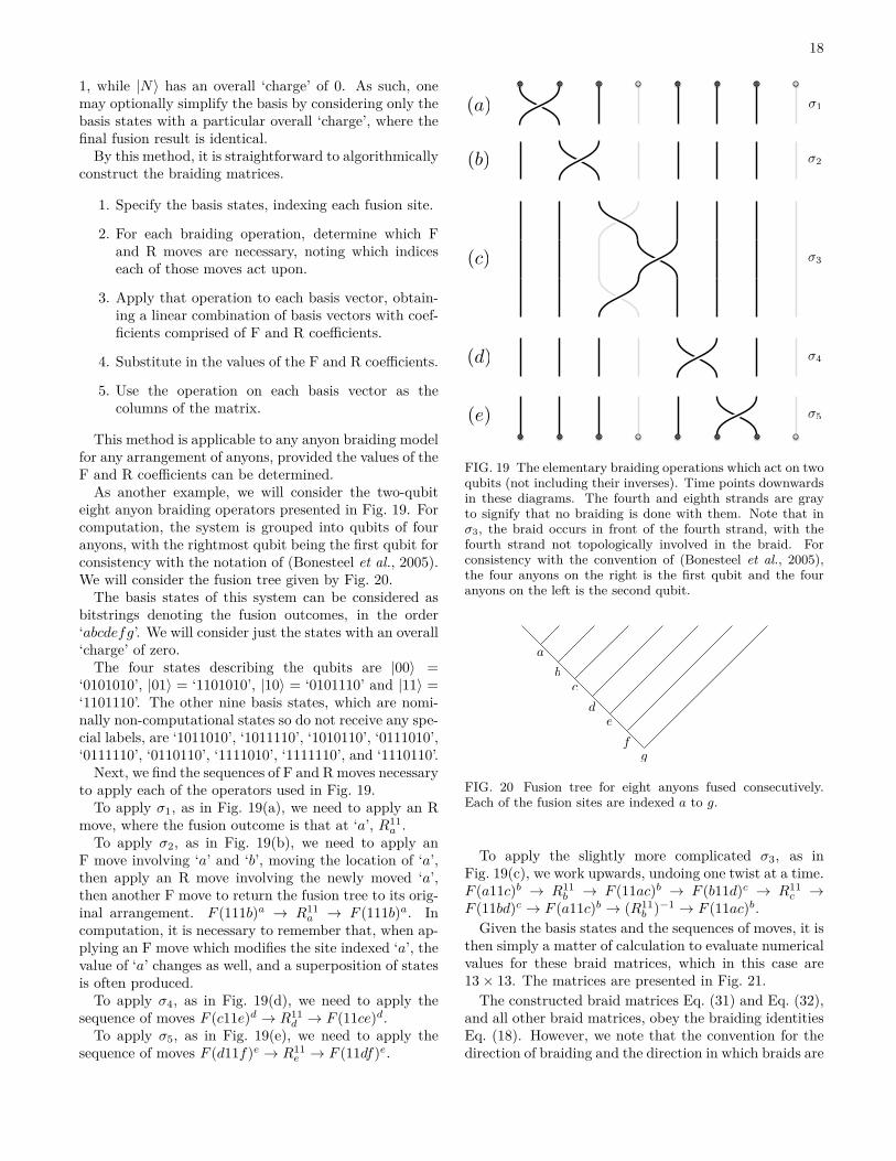
Explicit matrix representations for the effect of braid-ing can be constructed by performing F and R moves act-ing on an appropriate basis state (Preskill, 2004). Themethodology here can be used for any anyon model oncethe F and R coefficients have been determined. For con-creteness, we will apply this method to Fibonacci anyons.The first step is to choose the basis to work in. We will

consider the basis where the anyons are fused sequentiallyfrom left to right. For the purpose of demonstration wewill consider the case of three Fibonacci anyons, althoughthe method can readily be expanded to more.The next step is to enumerate over the possible basis

states. There are several possible representations. Onerepresentation is with circle notation, as in Fig. 18(a)-(c), or fusion trees, as in Fig. 18(d)-(f). The tree rep-resentation explicitly demonstrates the action of the Fand R moves, although for computation it is often moreuseful to represent the bases as bitstrings, where eachcomponent of the bitstring relates to a particular fusionoutcome. The action of an F move in this representationis to change one of the bits, and it is implied that theunderlying basis has also changed. Another representa-tion is to label the basis states with unique names. Forreasons that are explained in Section V.C, we label thestates in Fig. 18 as |0〉, |1〉 and |N〉. These states forman orthonormal set of basis vectors in C3.The next step is to consider the braid that we wish to

apply, then apply an appropriate sequence of F and Rmoves in order to convert that braid into a linear combi-nation of our chosen basis states. We must do this for thebraid acting on each of the possible basis states. Thus,

17

1

0 1

01

1

(a)

(d)

(b)

(e)

(c)

(f)

10

11 1

0

FIG. 18 Representations of the basis states of the 3 anyonsystem, where (a) and (d) are the same anyons, as are (b)and (e), and (c) and (f). As bitstrings, these states can berepresented as ‘01’, ‘11’ and ‘10’ respectively. The labels forthese states are |0〉, |1〉 and |N〉 respectively.

by considering the action of the operation upon each ofthe basis vectors, the matrix specifying that operationcan be constructed. We shall call the exchange of thefirst and second anyons σ1, and the exchange of the sec-

ond and third anyons σ2. The braid matrix σ1 can thusbe constructed element by element as

σ1|0〉 =1

0

= R110

1

0= e−4πi/5|0〉,

σ1|1〉 =1

1

= R111

1

1= e3πi/5|1〉,

σ1|N〉 =1

0

= R111 1

0

= e3πi/5|N〉,

resulting in the diagonal braid matrix

σ1 =

e−4πi/5 0 00 e3πi/5 00 0 e3πi/5

. (31)

Similarly, the braid matrix σ2 can be constructed as

σ2|0〉 =1

0

= F (1111)00

1

0

+ F (1111)01

1

1

= F (1111)00R

110

1

0+ F (1111)0

1R111

1

1

= F (1111)00R

110 F (1111)0

01

0+ F (1111)0

0R110 F (1111)0

11

1

+F (1111)01R

111 F (1111)1

01

0+ F (1111)0

1R111 F (1111)1

11

1

= (φ−2e−4πi/5 + φ−1e3πi/5)|0〉+ (φ−3/2e−4πi/5 − φ−3/2e3πi/5)|1〉 = φ−1e4πi/5|0〉+ φ−1/2e−3πi/5|1〉,

σ2|1〉 =1

1

= F (1111)10

1

0

+ F (1111)11

1

1

= F (1111)10R

110

1

0+ F (1111)1

1R111

1

1

= F (1111)10R

110 F (1111)0

01

0+ F (1111)1

0R110 F (1111)0

11

1

+F (1111)11R

111 F (1111)1

01

0+ F (1111)1

1R111 F (1111)1

11

1

= (φ−3/2e−4πi/5 − φ−3/2e3πi/5)|0〉+ (φ−1e−4πi/5 + φ−2e3πi/5)|1〉 = φ−1/2e−3πi/5|0〉 − φ−1|1〉,

σ2|N〉 =1

0

= F (1110)11

1

0

= F (1110)11R

111

1

0

= F (1110)11R

111 F (1110)1

1 1

0

= e3πi/5|N〉,

resulting in the block diagonal braid matrix

σ2 =

φ−1e4πi/5 φ−1/2e−3πi/5 0φ−1/2e−3πi/5 −φ−1 0

0 0 e3πi/5

. (32)

Note that the matrices Eq. (31) and Eq. (32) are blockdiagonal, and the braiding matrices for larger numbersof anyons are also block diagonal. It is not possible forbraiding to convert a |0〉 or |1〉 into an |N〉 or vice versa.This is because |0〉 and |1〉 have an overall ‘charge’ of

18

1, while |N〉 has an overall ‘charge’ of 0. As such, onemay optionally simplify the basis by considering only thebasis states with a particular overall ‘charge’, where thefinal fusion result is identical.

By this method, it is straightforward to algorithmicallyconstruct the braiding matrices.

1. Specify the basis states, indexing each fusion site.

2. For each braiding operation, determine which Fand R moves are necessary, noting which indiceseach of those moves act upon.

3. Apply that operation to each basis vector, obtain-ing a linear combination of basis vectors with coef-ficients comprised of F and R coefficients.

4. Substitute in the values of the F and R coefficients.

5. Use the operation on each basis vector as thecolumns of the matrix.

This method is applicable to any anyon braiding modelfor any arrangement of anyons, provided the values of theF and R coefficients can be determined.

As another example, we will consider the two-qubiteight anyon braiding operators presented in Fig. 19. Forcomputation, the system is grouped into qubits of fouranyons, with the rightmost qubit being the first qubit forconsistency with the notation of (Bonesteel et al., 2005).We will consider the fusion tree given by Fig. 20.

The basis states of this system can be considered asbitstrings denoting the fusion outcomes, in the order‘abcdefg’. We will consider just the states with an overall‘charge’ of zero.

The four states describing the qubits are |00〉 =‘0101010’, |01〉 = ‘1101010’, |10〉 = ‘0101110’ and |11〉 =‘1101110’. The other nine basis states, which are nomi-nally non-computational states so do not receive any spe-cial labels, are ‘1011010’, ‘1011110’, ‘1010110’, ‘0111010’,‘0111110’, ‘0110110’, ‘1111010’, ‘1111110’, and ‘1110110’.

Next, we find the sequences of F and R moves necessaryto apply each of the operators used in Fig. 19.

To apply σ1, as in Fig. 19(a), we need to apply an Rmove, where the fusion outcome is that at ‘a’, R11

a .To apply σ2, as in Fig. 19(b), we need to apply an

F move involving ‘a’ and ‘b’, moving the location of ‘a’,then apply an R move involving the newly moved ‘a’,then another F move to return the fusion tree to its orig-inal arrangement. F (111b)a → R11

a → F (111b)a. Incomputation, it is necessary to remember that, when ap-plying an F move which modifies the site indexed ‘a’, thevalue of ‘a’ changes as well, and a superposition of statesis often produced.

To apply σ4, as in Fig. 19(d), we need to apply thesequence of moves F (c11e)d → R11

d → F (11ce)d.To apply σ5, as in Fig. 19(e), we need to apply the

sequence of moves F (d11f)e → R11e → F (11df)e.

�1

�2

�3

�4

�5

(a)

(b)

(c)

(d)

(e)

FIG. 19 The elementary braiding operations which act on twoqubits (not including their inverses). Time points downwardsin these diagrams. The fourth and eighth strands are grayto signify that no braiding is done with them. Note that inσ3, the braid occurs in front of the fourth strand, with thefourth strand not topologically involved in the braid. Forconsistency with the convention of (Bonesteel et al., 2005),the four anyons on the right is the first qubit and the fouranyons on the left is the second qubit.

a

bc

de

fg

FIG. 20 Fusion tree for eight anyons fused consecutively.Each of the fusion sites are indexed a to g.

To apply the slightly more complicated σ3, as inFig. 19(c), we work upwards, undoing one twist at a time.F (a11c)b → R11

b → F (11ac)b → F (b11d)c → R11c →

F (11bd)c → F (a11c)b → (R11b )−1 → F (11ac)b.

Given the basis states and the sequences of moves, it isthen simply a matter of calculation to evaluate numericalvalues for these braid matrices, which in this case are13× 13. The matrices are presented in Fig. 21.The constructed braid matrices Eq. (31) and Eq. (32),

and all other braid matrices, obey the braiding identitiesEq. (18). However, we note that the convention for thedirection of braiding and the direction in which braids are

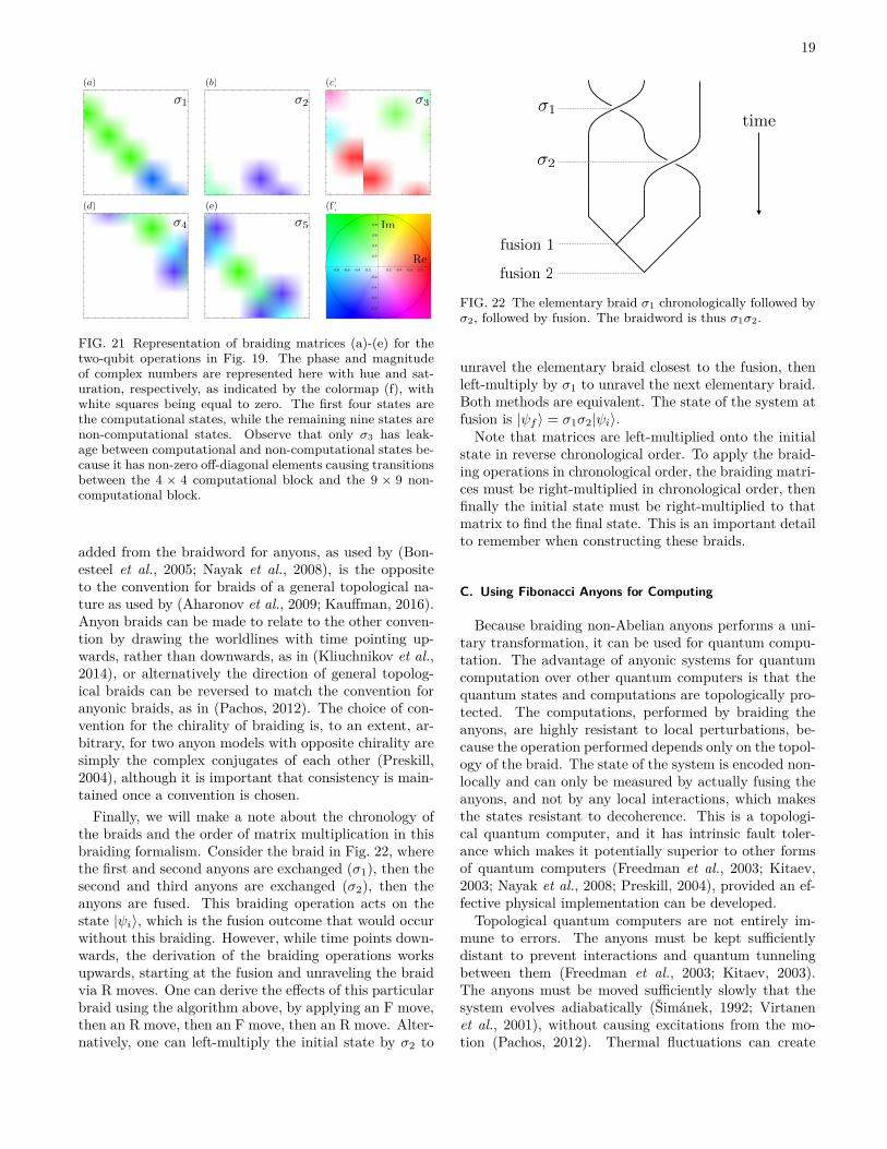
19

(a) (b) (c)

(d) (e) (f)

�1 �2 �3

�4 �5

-0.8 -0.6 -0.4 -0.2 0.2 0.4 0.6 0.8

-0.8

-0.6

-0.4

-0.2

0.2

0.4

0.6

0.8 Im

Re

FIG. 21 Representation of braiding matrices (a)-(e) for thetwo-qubit operations in Fig. 19. The phase and magnitudeof complex numbers are represented here with hue and sat-uration, respectively, as indicated by the colormap (f), withwhite squares being equal to zero. The first four states arethe computational states, while the remaining nine states arenon-computational states. Observe that only σ3 has leak-age between computational and non-computational states be-cause it has non-zero off-diagonal elements causing transitionsbetween the 4 × 4 computational block and the 9 × 9 non-computational block.

added from the braidword for anyons, as used by (Bon-esteel et al., 2005; Nayak et al., 2008), is the oppositeto the convention for braids of a general topological na-ture as used by (Aharonov et al., 2009; Kauffman, 2016).Anyon braids can be made to relate to the other conven-tion by drawing the worldlines with time pointing up-wards, rather than downwards, as in (Kliuchnikov et al.,2014), or alternatively the direction of general topolog-ical braids can be reversed to match the convention foranyonic braids, as in (Pachos, 2012). The choice of con-vention for the chirality of braiding is, to an extent, ar-bitrary, for two anyon models with opposite chirality aresimply the complex conjugates of each other (Preskill,2004), although it is important that consistency is main-tained once a convention is chosen.

Finally, we will make a note about the chronology ofthe braids and the order of matrix multiplication in thisbraiding formalism. Consider the braid in Fig. 22, wherethe first and second anyons are exchanged (σ1), then thesecond and third anyons are exchanged (σ2), then theanyons are fused. This braiding operation acts on thestate |ψi〉, which is the fusion outcome that would occurwithout this braiding. However, while time points down-wards, the derivation of the braiding operations worksupwards, starting at the fusion and unraveling the braidvia R moves. One can derive the effects of this particularbraid using the algorithm above, by applying an F move,then an R move, then an F move, then an R move. Alter-natively, one can left-multiply the initial state by σ2 to

�1

�2

fusion 1

fusion 2

time

FIG. 22 The elementary braid σ1 chronologically followed byσ2, followed by fusion. The braidword is thus σ1σ2.

unravel the elementary braid closest to the fusion, thenleft-multiply by σ1 to unravel the next elementary braid.Both methods are equivalent. The state of the system atfusion is |ψf 〉 = σ1σ2|ψi〉.Note that matrices are left-multiplied onto the initial

state in reverse chronological order. To apply the braid-ing operations in chronological order, the braiding matri-ces must be right-multiplied in chronological order, thenfinally the initial state must be right-multiplied to thatmatrix to find the final state. This is an important detailto remember when constructing these braids.

C. Using Fibonacci Anyons for Computing

Because braiding non-Abelian anyons performs a uni-tary transformation, it can be used for quantum compu-tation. The advantage of anyonic systems for quantumcomputation over other quantum computers is that thequantum states and computations are topologically pro-tected. The computations, performed by braiding theanyons, are highly resistant to local perturbations, be-cause the operation performed depends only on the topol-ogy of the braid. The state of the system is encoded non-locally and can only be measured by actually fusing theanyons, and not by any local interactions, which makesthe states resistant to decoherence. This is a topologi-cal quantum computer, and it has intrinsic fault toler-ance which makes it potentially superior to other formsof quantum computers (Freedman et al., 2003; Kitaev,2003; Nayak et al., 2008; Preskill, 2004), provided an ef-fective physical implementation can be developed.Topological quantum computers are not entirely im-

mune to errors. The anyons must be kept sufficientlydistant to prevent interactions and quantum tunnelingbetween them (Freedman et al., 2003; Kitaev, 2003).The anyons must be moved sufficiently slowly that thesystem evolves adiabatically (Šimánek, 1992; Virtanenet al., 2001), without causing excitations from the mo-tion (Pachos, 2012). Thermal fluctuations can create

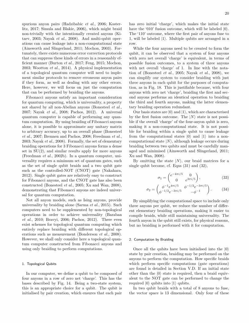
20

spurious anyon pairs (Hadzibabic et al., 2006; Koster-litz, 2017; Simula and Blakie, 2006), which might braidnon-trivially with the intentionally created anyons (Ki-taev, 2003; Nayak et al., 2008). And multi-qubit oper-ations can cause leakage into a non-computational state(Ainsworth and Slingerland, 2011; Mochon, 2003). For-tunately, there exists numerous error correction protocolsthat can suppress these kinds of errors in a reasonably ef-ficient manner (Burton et al., 2017; Feng, 2015; Mochon,2003; Wootton et al., 2014). A physical implementationof a topological quantum computer will need to imple-ment similar protocols to remove erroneous anyon pairsif they form, as well as dealing with any other errors.Here, however, we will focus on just the computationthat can be performed by braiding the anyons.

Fibonacci anyons satisfy an important considerationfor quantum computing, which is universality, a propertynot shared by all non-Abelian anyons (Bonesteel et al.,2007; Nayak et al., 2008; Pachos, 2012). A universalquantum computer is capable of performing any quan-tum computation. By using braiding of Fibonacci anyonsalone, it is possible to approximate any unitary matrixto arbitrary accuracy, up to an overall phase (Bonesteelet al., 2007; Brennen and Pachos, 2008; Freedman et al.,2003; Nayak et al., 2008). Formally, the set of elementarybraiding operations for 3 Fibonacci anyons forms a denseset in SU(2), and similar results apply for more anyons(Freedman et al., 2002b). In a quantum computer, uni-versality requires a minimum set of quantum gates, suchas the set of single qubit braids and a two qubit gatesuch as the controlled-NOT (CNOT) gate (Nakahara,2012). Single qubit gates are relatively easy to constructfor Fibonacci anyons, and the CNOT gate has also beenconstructed (Bonesteel et al., 2005; Xu and Wan, 2008),demonstrating that Fibonacci anyons are indeed univer-sal for quantum computation.

Not all anyon models, such as Ising anyons, provideuniversality by braiding alone (Sarma et al., 2015). Suchcomputers need to be supplemented by non-topologicaloperations in order to achieve universality (Barabanet al., 2010; Bravyi, 2006; Pachos, 2012). There evenexist schemes for topological quantum computing whichentirely replace braiding with different topological op-erations such as measurement (Bonderson et al., 2008).However, we shall only consider here a topological quan-tum computer constructed from Fibonacci anyons andusing only braiding to perform computations.

1. Topological Qubits

In our computer, we define a qubit to be composed offour anyons in a row of zero net ‘charge’. This has thebases described by Fig. 14. Being a two-state system,this is an appropriate choice for a qubit. The qubit isinitialised by pair creation, which ensures that each pair

has zero initial ‘charge’, which makes the initial statehave the ‘010’ fusion outcome, which will be labeled |0〉.The ‘110’ outcome, where the first pair of anyons fuse to1, will be labeled |1〉. Multiple qubits are arranged in arow.While the four anyons need to be created to form the

qubit, it can be observed that a system of four anyonswith zero net overall ‘charge’ is equivalent, in terms ofpossible fusion outcomes, to a system of three anyonswith net overall ‘charge’ of 1. In line with the nota-tion of (Bonesteel et al., 2005; Nayak et al., 2008), wecan simplify our system to consider braiding with justthree anyons in each qubit for the purposes of computa-tion, as in Fig. 18. This is justifiable because, with fouranyons with zero net ‘charge’, braiding the first and sec-ond anyons performs an identical operation to braidingthe third and fourth anyons, making the latter elemen-tary braiding operation redundant.Our basis states are |0〉 and |1〉, which are characterised

by the first fusion outcome. The |N〉 state is not possi-ble if the overall ‘charge’ of the four-anyon qubit is zero,making it a non-computational state. It is not possi-ble for braiding within a single qubit to cause leakagefrom the computational states |0〉 and |1〉 into a non-computational state |N〉, although leakage occurs duringbraiding between two qubits and must be carefully man-aged and minimised (Ainsworth and Slingerland, 2011;Xu and Wan, 2008).By omitting the state |N〉, our braid matrices for a

single qubit become, cf. Eqns (31) and (32),

σ1 =(e−4πi/5 0

0 e3πi/5

), (33)

σ2 =(

φ−1e4πi/5 φ−1/2e−3πi/5

φ−1/2e−3πi/5 −φ−1

). (34)

By simplifying the computational space to include onlythree anyons per qubit, we reduce the number of differ-ent elementary braiding operations, making it easier tocompile braids, while still maintaining universality. Thefourth anyon in the qubit still exists, for physical reasons,but no braiding is performed with it for computation.

2. Computation by Braiding

Once all the qubits have been initialised into the |0〉state by pair creation, braiding may be performed on theanyons to perform the computation. How specific braidswhich perform specific computations (gate operations)are found is detailed in Section V.D. If an initial stateother than the |0〉 state is required, then a braid equiv-alent to the NOT gate can be performed to change therequired |0〉 qubits into |1〉 qubits.In two qubit braids with a total of 8 anyons to fuse,

the vector space is 13 dimensional. Only four of these

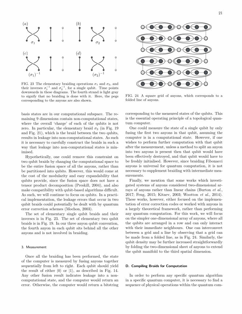
21

�1 �2

(�2)�1(�1)

�1

(a) (b)

(c) (d)

FIG. 23 The elementary braiding operations σ1 and σ2, andtheir inverses σ−1

1 and σ−12 , for a single qubit. Time points

downwards in these diagrams. The fourth strand is light grayto signify that no braiding is done with it. Here, the pegscorresponding to the anyons are also shown.

basis states are in our computational subspace. The re-maining 9 dimensions contain non-computational states,where the overall ‘charge’ of each of the qubits is notzero. In particular, the elementary braid σ3 (in Fig. 19and Fig. 21), which is the braid between the two qubits,results in leakage into non-computational states. As suchit is necessary to carefully construct the braids in such away that leakage into non-computational states is min-imised.

Hypothetically, one could remove this constraint ontwo qubit braids by changing the computational space tobe the entire fusion space of all the anyons, rather thanbe partitioned into qubits. However, this would come atthe cost of the modularity and easy expandability thatqubits provide, since the fusion space does not have atensor product decomposition (Preskill, 2004), and alsomake compatibility with qubit-based algorithms difficult.As such, we will continue to focus on qubits. In a practi-cal implementation, the leakage errors that occur in twoqubit braids could potentially be dealt with by quantumerror correction schemes (Mochon, 2003).

The set of elementary single qubit braids and theirinverses is in Fig. 23. The set of elementary two qubitbraids is in Fig. 19. In our three anyon qubit convention,the fourth anyon in each qubit sits behind all the otheranyons and is not involved in braiding.

3. Measurement

Once all the braiding has been performed, the stateof the computer is measured by fusing anyons togethersequentially from left to right. Each qubit should yieldthe result of either |0〉 or |1〉, as described in Fig. 14.Any other fusion result indicates leakage into a non-computational state, and the computer would return anerror. Otherwise, the computer would return a bitstring

FIG. 24 A square grid of anyons, which corresponds to afolded line of anyons.

corresponding to the measured states of the qubits. Thisis the essential operating principle of a topological quan-tum computer.One could measure the state of a single qubit by only

fusing the first two anyons in that qubit, assuming thecomputer is in a computational state. However, if onewishes to perform further computation with that qubitafter the measurement, unless a method to split an anyoninto two anyons is present then that qubit would havebeen effectively destroyed, and that qubit would have tobe freshly initialised. However, since braiding Fibonaccianyons is universal for quantum computation, it is notnecessary to supplement braiding with intermediate mea-surements.Finally, we mention that some works which investi-

gated systems of anyons considered two-dimensional ar-rays of anyons rather than linear chains (Burton et al.,2017; Feng, 2015; Kitaev, 2003; Wootton et al., 2014).These works, however, either focused on the implemen-tation of error correction codes or worked with anyons ina largely theoretical framework, rather than performingany quantum computation. For this work, we will focuson the simpler one-dimensional array of anyons, where allthe qubits are arranged in a row and can only interactwith their immediate neighbours. One can interconvertbetween a grid and a line by observing that a grid canbe made from a folded line, as in Fig. 24. Similarly, thequbit density may be further increased straightforwardlyby folding the two-dimensional sheet of anyons to extendthe qubit manifold to the third spatial dimension.

D. Compiling Braids for Computation

In order to perform any specific quantum algorithmin a specific quantum computer, it is necessary to find asequence of physical operations within the quantum com-

22

puter which approximates the required quantum gates forthat algorithm to a desired accuracy. In classical com-puters, this involves deciding how many bits to be usedto store each number, which determines the machine pre-cision. In the case of anyons, this sequence of physicaloperations is a braid. A braid which exactly implementsa given operation does not always exist, so approxima-tions are usually necessary (Freedman and Wang, 2007).While a braid approximating an arbitrary unitary matrixup to an overall phase to arbitrary accuracy theoreticallyexists, finding this braid is typically non-trivial.

1. Error Metrics

In searching for these braids, it is necessary to have ametric for how closely one matrix matches another. Thiscan be done using the operator norm of the differencebetween those two matrices (Bonesteel et al., 2005; Bur-rello et al., 2011; Xu and Wan, 2008). The operator normgives the largest value by which a matrix can change thelength of a vector. If two matrices are equal, then theirdifference will give the zero matrix, which has an oper-ator norm of zero. If two matrices are dissimilar, thentheir difference will be dissimilar to the zero matrix, andso have a larger operator norm. A smaller value for thiserror metric indicates a better approximation.

Explicitly, the operator norm can be evaluated using

||A|| =√

maxEigenvalue(A†A). (35)

It is also important to consider that, while Fibonaccibraiding forms a dense set in SU(2) (Freedman et al.,2002b), the group of 2 × 2 unitary matrices with a de-terminant of 1, it does not form a dense set in U(2),the group of arbitrary 2 × 2 unitary matrices. This canbe shown by observing that the determinants of the ele-mentary Fibonacci braiding matrices are all e±πi/5. Thismeans that the determinant of the matrix representingany braid is enπi/5, where n is some integer. This meansthat it is not possible for braiding of Fibonacci anyons toapproximate a unitary matrix which has another deter-minant. However, it is possible for braiding to approxi-mate that matrix times a certain overall phase factor.

The determinant of an arbitrary unitary matrix U isdet(U) = eiφ, and for demonstration purposes we shallassume that U is a 2× 2 matrix. We can change the de-terminant of U by multiplying it by a phase factor. Sup-pose we want to construct a certain unitary U ′, which isa member of SU(2) and differs from U only by an overallphase. Then det(U ′) = e−iφ det(U) = det(e−iφ/2U), soU ′ = e−iφ/2U . Therefore, it is possible to find braidswhich approximate any unitary matrix U up to an over-all phase factor. Since in quantum mechanics the overallphase of a system cannot be measured, this overall phaseis generally of no consequence.

When comparing how closely two matrices match usingthe operator norm, we require a way to cancel out thephase difference between the two unless we have alreadyguaranteed that both are within SU(2). The determinantof a 2×2 unitary matrix returns the square of the phase.This gives two possible solutions for the actual phaseof each unitary matrix, but one will provide the phasedifference between those two matrices, while the otherwill be off by a factor of −1. For using the operatornorm, we can compare both possible phase differencesand choose the one that results in the closest match.

While this provides the phase difference between thetwo matrices, it is relatively expensive computationally.A simpler method for comparing two 2×2 unitary matri-ces while ignoring their global phase is the global phaseinvariant distance defined by (Kliuchnikov et al., 2014),

d(U, V ) =√

1− |tr(UV †)| /2, (36)

where tr is the standard matrix trace, the sum of diagonalelements. This distance d(U, V ) gives a measure of thedifference between U and V while ignoring their overallphases. If U and V are equal and unitary, then UV † = I2.The trace of I2 is 2 (hence the division by 2, to normalisethe trace). Eq. (36) would then give a value of zero. IfU = eiφV , then UV † = eiφI2, so the trace is 2eiφ, andthe absolute value of the trace will be 2, which would alsolead to a distance of zero. As such, Eq. (36) is insensitiveto the global phase of the matrices.

However, it turns out that the global phase invariantdistance and the operator norm after global phases havebeen removed are actually equivalent, up to a normalisa-tion constant of

√2.

Consider the unitary matrices A,B ∈ SU(2). Notethat −B is also a member of SU(2). As such, when find-ing the operator norm of the difference between thesetwo matrices while ignoring the global phase betweenthem, we will want to take the minimum of ||A−B||and ||A+B||, such that

||A∓B|| =√

Eig[(A∓B)†(A∓B)]

=√

Eig[A†A+B†B ∓A†B ∓B†A].(37)

Let C = A†B. Note that C ∈ SU(2), so it is a matrix ofthe form

C =(

a b−b∗ a∗

), where |a|2 + |b|2 = 1. (38)

23

Hence,

||A∓B|| =√

Eig[2I∓ (C + C†)]

=

√Eig

(2∓ (a+ a∗) b− bb∗ − b∗ 2∓ (a∗ + a)

)

=

√Eig

(2∓ 2 Re(a) 0

0 2∓ 2 Re(a)

)=√

2∓ 2 Re(a).

(39)

Taking the minimum of Eq. (39), we obtain

||A∓B|| =√

2− 2 |Re(a)|. (40)

Now consider the global phase invariant distance.√

2d(A,B) =√

2− |tr(AB†)|

=√

2− |tr(B†A)| =√

2− |tr(C†)|=√

2− |a∗ + a| =√

2− 2 |Re(a)|.

(41)

Since Eq. (40) and Eq. (41) are the same, this provesthat these two apparently different metrics are actuallythe same. The computational advantage of Eq. (36) isthat it removes any global phase difference between thetwo matrices in a facile manner, but both will producethe same result up to a normalisation constant.

For consistency with (Bonesteel et al., 2005), we willreport errors of braids with the normalisation inherent tothe operator norm, which is

√2 times more than Eq. (36).

2. Compiling Single Qubit Braids

The simplest method for finding a braid which approx-imates a given unitary is by an exhaustive search, check-ing each possible braidword up to a certain length to seeif it constructs the desired unitary matrix to within a de-sired accuracy. Exhaustive search was the method usedin this work to find braids. The time taken for this bruteforce method grows exponentially as O(bL), where b isthe number of elementary operations in the search and Lis the length of the braid.

There are several optimisations we made to make theexhaustive search more efficient. Most of these op-timisations work on eliminating braidwords which areequivalent to previously investigated braidwords from thesearch. If an elementary braid and its inverse were ad-jacent to each other, the braid was rejected. By notingthat, for Fibonacci anyons, σ6

i = σ−4i (or, equivalently,

σ10i = I), any braidword with six or more consecutive

identical elements was rejected. Due to topology andbraiding identities, it was noted that certain triplets ofelementary braids were equivalent to other triplets (eg.σ1σ2σ1 = σ2σ1σ2, σ2σ1σ

−12 = σ−1

1 σ2σ1), so from each

pair only one pattern was kept while the other rejected.In certain cases, applying these equivalences would resultin cancellation from adjacent inverses, which led to a se-lection of four element patterns which were also rejected.By these optimisations, we reduced the number of braid-words of length 18 or less to 33,527,163, which is a tinyfraction of the potential 91,625,968,980 braidwords.There are two more optimisations that were made, per-

taining to trading memory for speed. Generating braid-words of length n can be done by appending elements tothe end of the valid braidwords of length n − 1. Thisavoids generating many braidwords which contain pat-terns which would lead to them being rejected for re-dundancy, at the cost of using more memory since thebraids have to be recorded. However, using the other op-timisations, the memory requirements were not onerous.Finally, the generated valid braidwords could be savedto file and retrieved later, saving on computation at latertimes.A special sub-class of braids are weaves, where one

strand, the warp strand, moves around other stationarystrands, the weft strands (Simon et al., 2006). For braid-ing anyons, this can be achieved by moving one anyonwhile keeping the other anyons stationary. It has beenshown that any operation which can be performed with abraid can also be performed with a weave (Simon et al.,2006). Furthermore, it has also been shown that, in thethree anyon case, weaves with the warp starting and fin-ishing at the middle position (with generators σ±2

1 andσ±2

2 ) also forms a dense set in SU(2) (Bonesteel et al.,2007), meaning such weaves can approximate any arbi-trary unitary operation up to an overall phase. An exam-ple of a weave approximating a matrix is given in Fig. 25.

Using the elementary weaving operations σ±21 and σ±2

2 ,an exhaustive search for single qubit weaves is similarto the exhaustive search for single qubit braids. In-verses could be canceled as before. There were no sim-ple topologically equivalent patterns as for braids. How-ever, (σ2

i )3 = (σ−2i )2, meaning that any braidword with

three or more consecutive identical elementary weavescould be rejected. For braidwords with up to 18 el-ementary weaving operations (which corresponds to 36elementary braiding operations), these optimisations re-duced the number of braidwords from 91,625,968,980 to178,918,056.Given the braidword approximating an operation, the

inverse can be found by simply reversing the order andinverting the signs of the powers of the braidword.

3. Convergence of Single Qubit Braids

When searching for braids which approximate a tar-get operation, it is important that these braids con-verge quickly. If increasing the desired accuracy requiresincreasing the length of the braid by an exponential

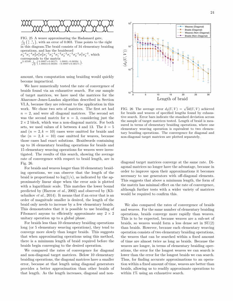
24

FIG. 25 A weave approximating the Hadamard gate,1√2

(1 11 −1

), with an error of 0.003. Time points to the right

in this diagram.The braid consists of 34 elementary braidingoperations, and has the braidwordσ−4

2 σ−41 σ2

2σ41σ

22σ−21 σ−4

2 σ−21 σ−2

2 σ−21 σ−2

2 σ21σ−22 , which

corresponds to the matrixe3.4558i 1√

2

( 0.9997+0.0017i 1.0003−0.0039i1.0003+0.0039i −0.9997+0.0017i

).

amount, then computation using braiding would quicklybecome impractical.

We have numerically tested the rate of convergence ofbraids found via an exhaustive search. For our sampleof target matrices, we have used the matrices for theAharonov-Jones-Landau algorithm described in SectionVI.A, because they are relevant to the application in thiswork. We chose two sets of matrices. The first set hadn = 2, and were all diagonal matrices. The second setwas the second matrix for n = 3, considering just the2× 2 block, which was a non-diagonal matrix. For bothsets, we used values of k between 4 and 13. The k = 5and (n = 2, k = 10) cases were omitted for braids andthe (n = 2, k = 10) case omitted for weaves, becausethose cases had exact solutions. Braidwords containingup to 16 elementary braiding operations for braids and15 elementary weaving operations for weaves were inves-tigated. The results of this search, showing the averagerate of convergence with respect to braid length, are inFig. 26.

For braids and weaves longer than 10 elementary braid-ing operations, we can observe that the length of thebraid is proportional to log(1/ε), as indicated by the ap-proximately linear slope when the error axis is plottedwith a logarithmic scale. This matches the lower boundpredicted by (Harrow et al., 2002) and observed by (Kli-uchnikov et al., 2014). It means that if an error that is anorder of magnitude smaller is desired, the length of thebraid only needs to increase by a few elementary braids.This demonstrates that it is possible to use braiding ofFibonacci anyons to efficiently approximate any 2 × 2unitary operation up to a global phase.

For braids less than 10 elementary braiding operationslong (or 5 elementary weaving operations), they tend toconverge more slowly than longer braids. This suggeststhat when approximating operations using this method,there is a minimum length of braid required before thebraids begin converging to the desired operation.

We compared the rates of convergence for diagonaland non-diagonal target matrices. Below 10 elementarybraiding operations, the diagonal matrices have a smallererror, because at that length using diagonal generatorsprovides a better approximation than other braids ofthat length. As the length increases, diagonal and non-

0 5 10 15 20 25 3010−3

10−2

10−1

100

Weaves (Diagonal)Braids (Diagonal)Weaves (Non−Diagonal)Braids (Non−Diagonal)

Length of braid

hd2(U

,V)i

FIG. 26 The average error d2(U, V ) =√

2d(U, V ) achievedfor braids and weaves of specified lengths found by exhaus-tive search. Error bars indicate the standard deviation acrossthe sample of target matrices tested. Length of braid is mea-sured in terms of elementary braiding operations, where oneelementary weaving operation is equivalent to two elemen-tary braiding operations. The convergence for diagonal andnon-diagonal target matrices are plotted separately.

diagonal target matrices converge at the same rate. Di-agonal matrices no longer have the advantage, because inorder to improve upon their approximations it becomesnecessary to use generators with off-diagonal elements.This suggests that above a minimum length, the form ofthe matrix has minimal effect on the rate of convergence,although further tests with a wider variety of matriceswould be required to confirm this.

We also compared the rates of convergence of braidsand weaves. For the same number of elementary braidingoperations, braids converge more rapidly than weaves.This is to be expected, because weaves are a sub-set ofbraids, so weaves would form a less dense set in SU(2)than braids. However, because each elementary weavingoperation consists of two elementary braiding operations,the weaves that can be searched within a fixed amountof time are almost twice as long as braids. Because theweaves are longer, in terms of elementary braiding oper-ations, the error for the longest weaves we can search islower than the error for the longest braids we can search.Thus, for finding accurate approximations to an opera-tion within a fixed amount of time, weaves are better thanbraids, allowing us to readily approximate operations towithin 1% using an exhaustive search.

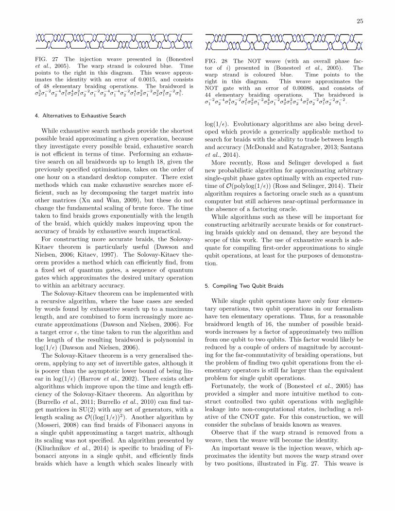
25

FIG. 27 The injection weave presented in (Bonesteelet al., 2005). The warp strand is coloured blue. Timepoints to the right in this diagram. This weave approx-imates the identity with an error of 0.0015, and consistsof 48 elementary braiding operations. The braidword isσ3

2σ−21 σ−4

2 σ21σ

42σ

21σ−22 σ−2

1 σ−42 σ−4

1 σ−22 σ4

1σ22σ−21 σ2

2σ21σ−22 σ3

1 .

4. Alternatives to Exhaustive Search

While exhaustive search methods provide the shortestpossible braid approximating a given operation, becausethey investigate every possible braid, exhaustive searchis not efficient in terms of time. Performing an exhaus-tive search on all braidwords up to length 18, given thepreviously specified optimisations, takes on the order ofone hour on a standard desktop computer. There existmethods which can make exhaustive searches more ef-ficient, such as by decomposing the target matrix intoother matrices (Xu and Wan, 2009), but these do notchange the fundamental scaling of brute force. The timetaken to find braids grows exponentially with the lengthof the braid, which quickly makes improving upon theaccuracy of braids by exhaustive search impractical.

For constructing more accurate braids, the Solovay-Kitaev theorem is particularly useful (Dawson andNielsen, 2006; Kitaev, 1997). The Solovay-Kitaev the-orem provides a method which can efficiently find, froma fixed set of quantum gates, a sequence of quantumgates which approximates the desired unitary operationto within an arbitrary accuracy.

The Solovay-Kitaev theorem can be implemented witha recursive algorithm, where the base cases are seededby words found by exhaustive search up to a maximumlength, and are combined to form increasingly more ac-curate approximations (Dawson and Nielsen, 2006). Fora target error ε, the time taken to run the algorithm andthe length of the resulting braidword is polynomial inlog(1/ε) (Dawson and Nielsen, 2006).The Solovay-Kitaev theorem is a very generalised the-

orem, applying to any set of invertible gates, although itis poorer than the asymptotic lower bound of being lin-ear in log(1/ε) (Harrow et al., 2002). There exists otheralgorithms which improve upon the time and length effi-ciency of the Solovay-Kitaev theorem. An algorithm by(Burrello et al., 2011; Burrello et al., 2010) can find tar-get matrices in SU(2) with any set of generators, with alength scaling as O((log(1/ε))2). Another algorithm by(Mosseri, 2008) can find braids of Fibonacci anyons ina single qubit approximating a target matrix, althoughits scaling was not specified. An algorithm presented by(Kliuchnikov et al., 2014) is specific to braiding of Fi-bonacci anyons in a single qubit, and efficiently findsbraids which have a length which scales linearly with

FIG. 28 The NOT weave (with an overall phase fac-tor of i) presented in (Bonesteel et al., 2005). Thewarp strand is coloured blue. Time points to theright in this diagram. This weave approximates theNOT gate with an error of 0.00086, and consists of44 elementary braiding operations. The braidword isσ−2

1 σ−42 σ4

1σ−22 σ2

1σ22σ−21 σ4

2σ−21 σ4

2σ21σ−42 σ2

1σ−22 σ2

1σ−22 σ−2

1 .

log(1/ε). Evolutionary algorithms are also being devel-oped which provide a generically applicable method tosearch for braids with the ability to trade between lengthand accuracy (McDonald and Katzgraber, 2013; Santanaet al., 2014).More recently, Ross and Selinger developed a fast

new probabilistic algorithm for approximating arbitrarysingle-qubit phase gates optimally with an expected run-time of O(polylog(1/ε)) (Ross and Selinger, 2014). Theiralgorithm requires a factoring oracle such as a quantumcomputer but still achieves near-optimal performance inthe absence of a factoring oracle.While algorithms such as these will be important for

constructing arbitrarily accurate braids or for construct-ing braids quickly and on demand, they are beyond thescope of this work. The use of exhaustive search is ade-quate for compiling first-order approximations to singlequbit operations, at least for the purposes of demonstra-tion.

5. Compiling Two Qubit Braids

While single qubit operations have only four elemen-tary operations, two qubit operations in our formalismhave ten elementary operations. Thus, for a reasonablebraidword length of 16, the number of possible braid-words increases by a factor of approximately two millionfrom one qubit to two qubits. This factor would likely bereduced by a couple of orders of magnitude by account-ing for the far-commutativity of braiding operations, butthe problem of finding two qubit operations from the el-ementary operators is still far larger than the equivalentproblem for single qubit operations.Fortunately, the work of (Bonesteel et al., 2005) has

provided a simpler and more intuitive method to con-struct controlled two qubit operations with negligibleleakage into non-computational states, including a rel-ative of the CNOT gate. For this construction, we willconsider the subclass of braids known as weaves.Observe that if the warp strand is removed from a

weave, then the weave will become the identity.An important weave is the injection weave, which ap-

proximates the identity but moves the warp strand overby two positions, illustrated in Fig. 27. This weave is

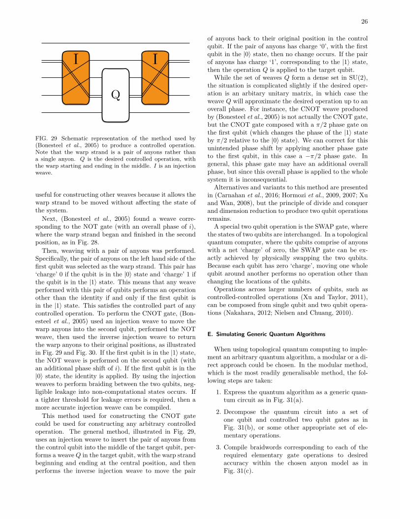
26

I

Q

I

FIG. 29 Schematic representation of the method used by(Bonesteel et al., 2005) to produce a controlled operation.Note that the warp strand is a pair of anyons rather thana single anyon. Q is the desired controlled operation, withthe warp starting and ending in the middle. I is an injectionweave.

useful for constructing other weaves because it allows thewarp strand to be moved without affecting the state ofthe system.

Next, (Bonesteel et al., 2005) found a weave corre-sponding to the NOT gate (with an overall phase of i),where the warp strand began and finished in the secondposition, as in Fig. 28.

Then, weaving with a pair of anyons was performed.Specifically, the pair of anyons on the left hand side of thefirst qubit was selected as the warp strand. This pair has‘charge’ 0 if the qubit is in the |0〉 state and ‘charge’ 1 ifthe qubit is in the |1〉 state. This means that any weaveperformed with this pair of qubits performs an operationother than the identity if and only if the first qubit isin the |1〉 state. This satisfies the controlled part of anycontrolled operation. To perform the CNOT gate, (Bon-esteel et al., 2005) used an injection weave to move thewarp anyons into the second qubit, performed the NOTweave, then used the inverse injection weave to returnthe warp anyons to their original positions, as illustratedin Fig. 29 and Fig. 30. If the first qubit is in the |1〉 state,the NOT weave is performed on the second qubit (withan additional phase shift of i). If the first qubit is in the|0〉 state, the identity is applied. By using the injectionweaves to perform braiding between the two qubits, neg-ligible leakage into non-computational states occurs. Ifa tighter threshold for leakage errors is required, then amore accurate injection weave can be compiled.

This method used for constructing the CNOT gatecould be used for constructing any arbitrary controlledoperation. The general method, illustrated in Fig. 29,uses an injection weave to insert the pair of anyons fromthe control qubit into the middle of the target qubit, per-forms a weave Q in the target qubit, with the warp strandbeginning and ending at the central position, and thenperforms the inverse injection weave to move the pair

of anyons back to their original position in the controlqubit. If the pair of anyons has charge ‘0’, with the firstqubit in the |0〉 state, then no change occurs. If the pairof anyons has charge ‘1’, corresponding to the |1〉 state,then the operation Q is applied to the target qubit.While the set of weaves Q form a dense set in SU(2),

the situation is complicated slightly if the desired oper-ation is an arbitary unitary matrix, in which case theweave Q will approximate the desired operation up to anoverall phase. For instance, the CNOT weave producedby (Bonesteel et al., 2005) is not actually the CNOT gate,but the CNOT gate composed with a π/2 phase gate onthe first qubit (which changes the phase of the |1〉 stateby π/2 relative to the |0〉 state). We can correct for thisunintended phase shift by applying another phase gateto the first qubit, in this case a −π/2 phase gate. Ingeneral, this phase gate may have an additional overallphase, but since this overall phase is applied to the wholesystem it is inconsequential.Alternatives and variants to this method are presented

in (Carnahan et al., 2016; Hormozi et al., 2009, 2007; Xuand Wan, 2008), but the principle of divide and conquerand dimension reduction to produce two qubit operationsremains.A special two qubit operation is the SWAP gate, where

the states of two qubits are interchanged. In a topologicalquantum computer, where the qubits comprise of anyonswith a net ‘charge’ of zero, the SWAP gate can be ex-actly achieved by physically swapping the two qubits.Because each qubit has zero ‘charge’, moving one wholequbit around another performs no operation other thanchanging the locations of the qubits.Operations across larger numbers of qubits, such as

controlled-controlled operations (Xu and Taylor, 2011),can be composed from single qubit and two qubit opera-tions (Nakahara, 2012; Nielsen and Chuang, 2010).

E. Simulating Generic Quantum Algorithms

When using topological quantum computing to imple-ment an arbitrary quantum algorithm, a modular or a di-rect approach could be chosen. In the modular method,which is the most readily generalisable method, the fol-lowing steps are taken:

1. Express the quantum algorithm as a generic quan-tum circuit as in Fig. 31(a).

2. Decompose the quantum circuit into a set ofone qubit and controlled two qubit gates as inFig. 31(b), or some other appropriate set of ele-mentary operations.

3. Compile braidwords corresponding to each of therequired elementary gate operations to desiredaccuracy within the chosen anyon model as inFig. 31(c).

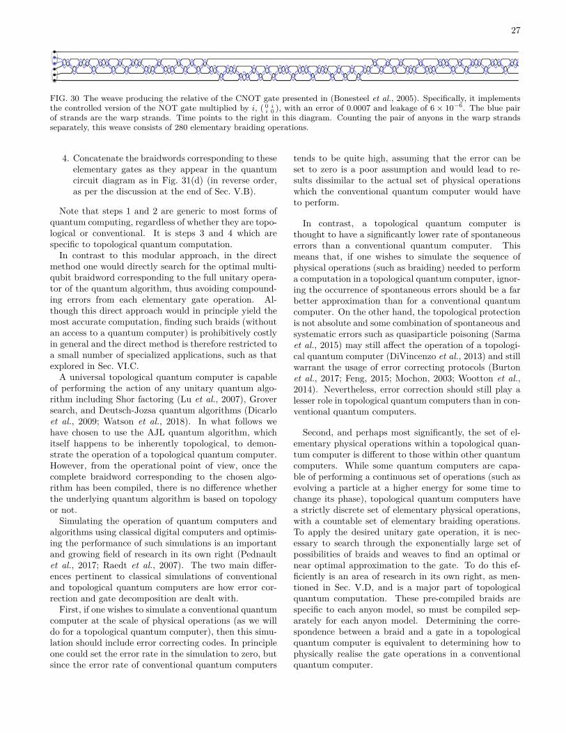
27

FIG. 30 The weave producing the relative of the CNOT gate presented in (Bonesteel et al., 2005). Specifically, it implementsthe controlled version of the NOT gate multiplied by i, ( 0 i

i 0 ), with an error of 0.0007 and leakage of 6× 10−6. The blue pairof strands are the warp strands. Time points to the right in this diagram. Counting the pair of anyons in the warp strandsseparately, this weave consists of 280 elementary braiding operations.

4. Concatenate the braidwords corresponding to theseelementary gates as they appear in the quantumcircuit diagram as in Fig. 31(d) (in reverse order,as per the discussion at the end of Sec. V.B).

Note that steps 1 and 2 are generic to most forms ofquantum computing, regardless of whether they are topo-logical or conventional. It is steps 3 and 4 which arespecific to topological quantum computation.

In contrast to this modular approach, in the directmethod one would directly search for the optimal multi-qubit braidword corresponding to the full unitary opera-tor of the quantum algorithm, thus avoiding compound-ing errors from each elementary gate operation. Al-though this direct approach would in principle yield themost accurate computation, finding such braids (withoutan access to a quantum computer) is prohibitively costlyin general and the direct method is therefore restricted toa small number of specialized applications, such as thatexplored in Sec. VI.C.

A universal topological quantum computer is capableof performing the action of any unitary quantum algo-rithm including Shor factoring (Lu et al., 2007), Groversearch, and Deutsch-Jozsa quantum algorithms (Dicarloet al., 2009; Watson et al., 2018). In what follows wehave chosen to use the AJL quantum algorithm, whichitself happens to be inherently topological, to demon-strate the operation of a topological quantum computer.However, from the operational point of view, once thecomplete braidword corresponding to the chosen algo-rithm has been compiled, there is no difference whetherthe underlying quantum algorithm is based on topologyor not.

Simulating the operation of quantum computers andalgorithms using classical digital computers and optimis-ing the performance of such simulations is an importantand growing field of research in its own right (Pednaultet al., 2017; Raedt et al., 2007). The two main differ-ences pertinent to classical simulations of conventionaland topological quantum computers are how error cor-rection and gate decomposition are dealt with.

First, if one wishes to simulate a conventional quantumcomputer at the scale of physical operations (as we willdo for a topological quantum computer), then this simu-lation should include error correcting codes. In principleone could set the error rate in the simulation to zero, butsince the error rate of conventional quantum computers

tends to be quite high, assuming that the error can beset to zero is a poor assumption and would lead to re-sults dissimilar to the actual set of physical operationswhich the conventional quantum computer would haveto perform.

In contrast, a topological quantum computer isthought to have a significantly lower rate of spontaneouserrors than a conventional quantum computer. Thismeans that, if one wishes to simulate the sequence ofphysical operations (such as braiding) needed to performa computation in a topological quantum computer, ignor-ing the occurrence of spontaneous errors should be a farbetter approximation than for a conventional quantumcomputer. On the other hand, the topological protectionis not absolute and some combination of spontaneous andsystematic errors such as quasiparticle poisoning (Sarmaet al., 2015) may still affect the operation of a topologi-cal quantum computer (DiVincenzo et al., 2013) and stillwarrant the usage of error correcting protocols (Burtonet al., 2017; Feng, 2015; Mochon, 2003; Wootton et al.,2014). Nevertheless, error correction should still play alesser role in topological quantum computers than in con-ventional quantum computers.

Second, and perhaps most significantly, the set of el-ementary physical operations within a topological quan-tum computer is different to those within other quantumcomputers. While some quantum computers are capa-ble of performing a continuous set of operations (such asevolving a particle at a higher energy for some time tochange its phase), topological quantum computers havea strictly discrete set of elementary physical operations,with a countable set of elementary braiding operations.To apply the desired unitary gate operation, it is nec-essary to search through the exponentially large set ofpossibilities of braids and weaves to find an optimal ornear optimal approximation to the gate. To do this ef-ficiently is an area of research in its own right, as men-tioned in Sec. V.D, and is a major part of topologicalquantum computation. These pre-compiled braids arespecific to each anyon model, so must be compiled sep-arately for each anyon model. Determining the corre-spondence between a braid and a gate in a topologicalquantum computer is equivalent to determining how tophysically realise the gate operations in a conventionalquantum computer.

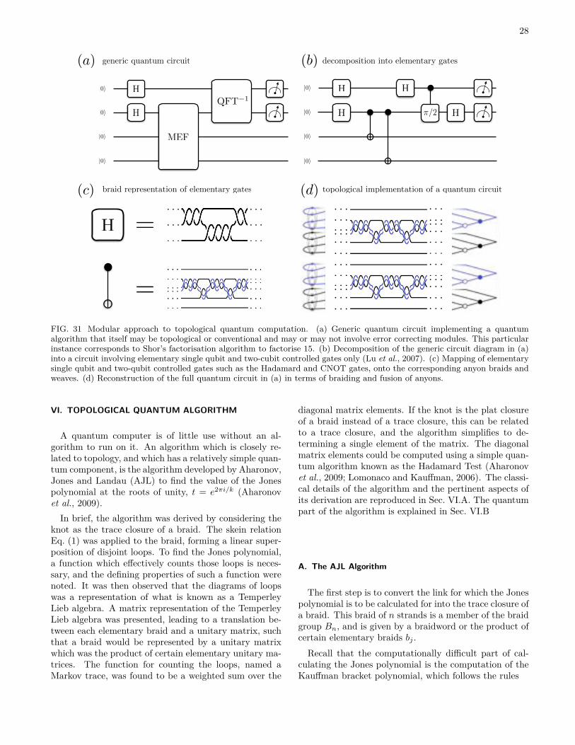
28

(a)

(c)

(b)

(d)

|0i H

|0i

|0i

|0i H

H

H ⇡/2

|0i

|0i

H

HQFT�1

MEF|0i

=

H =. . .

. . .

. . .

. . .

. . .

. . .

. . .

. . .

. . .

. . .

. . .

. . .. . .. . .

. . .

. . .. . .

. . .

39

FIG.42AbraidtypicalofacomputationintheAJLalgorithm.Inthisparticularbraid,theimaginarycomponentoftheseconddiagonalelementintheAJLmatrixproductcorrespondingtothetraceclosureofthepositiveHopflinkwithk=6isbeingmeasured.Ithasaleakageerrorof3.6◊10≠6.Thefirstqubitiscolouredblue.Thesecondqubitiscolouredblack.Thesegmentsmarkedas‘paired’indicatethattheweavehasbeenmodifiedsuchthattwoanyonsarebeingmovedinsteadofasingleanyon.Thestateoftheanyonsatthehollowcirclesinthemeasurementstepdeterminethestateofthequbit.

measured.Ifthefirstbitofthereturnedbitstringwas0,thentheHadamardtestreturned1.Ifthefirstbitwas1,thentheHadamardtestreturned≠1.Thiswasperformedforaspecifiednumberofiterationsforeachoftherealandimaginaryoutputs,andthemeanoftheoutputsforeachcomponentwastaken.ThisnumberwastheapproximationoftheMarkovtraceforthetraceclosureorthefirstmatrixelementfortheplatclosure.

Thewritheoftheknotwascalculatedclassically,andthentheappropriatefactorsweremultipliedtotheresultoftheHadamardtesttogiveanapproximationtotheJonespolynomialatthepointt=e2fii/k

.TheHadamardtestisstochasticinnature.Theresults

inTableIwereusedtoestimatetheconfidenceintervalsforagivenoutputoftheHadamardtest.Forthecon-fidenceintervalforthatpointintheJonespolynomial,thefigurefortheHadamardtestwasmultipliedbyd

n≠1

forthetraceclosureordn2≠1fortheplatclosure.Inour

results,wereportedthe95%confidenceintervalforeachdatapointintheJonespolynomialaserrorbars.

Becauseourquantumcomputerisaclassicalsimula-tion,wewereabletoaccessinformationthatwouldnotbemeasurableinarealquantumcomputer.Asamea-sureofcomparisontothestochasticresults,wedirectlyreadthecomponentsofthestatevectorandtheproba-bilityofmeasuringeachqubitinagivenstate,bypassingtherandomnatureofAlgorithm4.Thiswasusedtopre-ciselydeterminetheexpectationvalueoftheHadamardtestforagivensetofweavesinthequantumcomputer.This,inturn,gavetheoutputofthestochasticmeasure-mentsinthelimitofaninfinitenumberofiterations.Thisquantityisnota�ectedbythestochasticnatureoftheregularmeasurements,butitisa�ectedbyhowcloselythegivenweavesapproximatetheintendedoper-

39

FIG.42AbraidtypicalofacomputationintheAJLalgorithm.Inthisparticularbraid,theimaginarycomponentoftheseconddiagonalelementintheAJLmatrixproductcorrespondingtothetraceclosureofthepositiveHopflinkwithk=6isbeingmeasured.Ithasaleakageerrorof3.6◊10≠6.Thefirstqubitiscolouredblue.Thesecondqubitiscolouredblack.Thesegmentsmarkedas‘paired’indicatethattheweavehasbeenmodifiedsuchthattwoanyonsarebeingmovedinsteadofasingleanyon.Thestateoftheanyonsatthehollowcirclesinthemeasurementstepdeterminethestateofthequbit.

measured.Ifthefirstbitofthereturnedbitstringwas0,thentheHadamardtestreturned1.Ifthefirstbitwas1,thentheHadamardtestreturned≠1.Thiswasperformedforaspecifiednumberofiterationsforeachoftherealandimaginaryoutputs,andthemeanoftheoutputsforeachcomponentwastaken.ThisnumberwastheapproximationoftheMarkovtraceforthetraceclosureorthefirstmatrixelementfortheplatclosure.

Thewritheoftheknotwascalculatedclassically,andthentheappropriatefactorsweremultipliedtotheresultoftheHadamardtesttogiveanapproximationtotheJonespolynomialatthepointt=e2fii/k

.TheHadamardtestisstochasticinnature.Theresults

inTableIwereusedtoestimatetheconfidenceintervalsforagivenoutputoftheHadamardtest.Forthecon-fidenceintervalforthatpointintheJonespolynomial,thefigurefortheHadamardtestwasmultipliedbyd

n≠1

forthetraceclosureordn2≠1fortheplatclosure.Inour

results,wereportedthe95%confidenceintervalforeachdatapointintheJonespolynomialaserrorbars.

Becauseourquantumcomputerisaclassicalsimula-tion,wewereabletoaccessinformationthatwouldnotbemeasurableinarealquantumcomputer.Asamea-sureofcomparisontothestochasticresults,wedirectlyreadthecomponentsofthestatevectorandtheproba-bilityofmeasuringeachqubitinagivenstate,bypassingtherandomnatureofAlgorithm4.Thiswasusedtopre-ciselydeterminetheexpectationvalueoftheHadamardtestforagivensetofweavesinthequantumcomputer.This,inturn,gavetheoutputofthestochasticmeasure-mentsinthelimitofaninfinitenumberofiterations.Thisquantityisnota�ectedbythestochasticnatureoftheregularmeasurements,butitisa�ectedbyhowcloselythegivenweavesapproximatetheintendedoper-

. . .

. . .

. . .

. . .

. . .

. . .. . .. . .

. . .

. . .. . .

. . .

. . .

. . .

. . .

. . .

. . .

. . .. . .. . .

. . .

. . .. . .

. . .

39

FIG. 42 A braid typical of a computation in the AJL algorithm. In this particular braid, the imaginary component of thesecond diagonal element in the AJL matrix product corresponding to the trace closure of the positive Hopf link with k = 6is being measured. It has a leakage error of 3.6 ◊ 10≠6. The first qubit is coloured blue. The second qubit is coloured black.The segments marked as ‘paired’ indicate that the weave has been modified such that two anyons are being moved instead ofa single anyon. The state of the anyons at the hollow circles in the measurement step determine the state of the qubit.

measured. If the first bit of the returned bitstring was0, then the Hadamard test returned 1. If the first bitwas 1, then the Hadamard test returned ≠1. This wasperformed for a specified number of iterations for eachof the real and imaginary outputs, and the mean of theoutputs for each component was taken. This numberwas the approximation of the Markov trace for the traceclosure or the first matrix element for the plat closure.

The writhe of the knot was calculated classically, andthen the appropriate factors were multiplied to the resultof the Hadamard test to give an approximation to theJones polynomial at the point t = e2fii/k.

The Hadamard test is stochastic in nature. The resultsin Table I were used to estimate the confidence intervalsfor a given output of the Hadamard test. For the con-fidence interval for that point in the Jones polynomial,the figure for the Hadamard test was multiplied by dn≠1

for the trace closure or dn2 ≠1 for the plat closure. In our

results, we reported the 95% confidence interval for eachdata point in the Jones polynomial as error bars.

Because our quantum computer is a classical simula-tion, we were able to access information that would notbe measurable in a real quantum computer. As a mea-sure of comparison to the stochastic results, we directlyread the components of the state vector and the proba-bility of measuring each qubit in a given state, bypassingthe random nature of Algorithm 4. This was used to pre-cisely determine the expectation value of the Hadamardtest for a given set of weaves in the quantum computer.This, in turn, gave the output of the stochastic measure-ments in the limit of an infinite number of iterations.This quantity is not a�ected by the stochastic natureof the regular measurements, but it is a�ected by howclosely the given weaves approximate the intended oper-

39

FIG. 42 A braid typical of a computation in the AJL algorithm. In this particular braid, the imaginary component of thesecond diagonal element in the AJL matrix product corresponding to the trace closure of the positive Hopf link with k = 6is being measured. It has a leakage error of 3.6 ◊ 10≠6. The first qubit is coloured blue. The second qubit is coloured black.The segments marked as ‘paired’ indicate that the weave has been modified such that two anyons are being moved instead ofa single anyon. The state of the anyons at the hollow circles in the measurement step determine the state of the qubit.

measured. If the first bit of the returned bitstring was0, then the Hadamard test returned 1. If the first bitwas 1, then the Hadamard test returned ≠1. This wasperformed for a specified number of iterations for eachof the real and imaginary outputs, and the mean of theoutputs for each component was taken. This numberwas the approximation of the Markov trace for the traceclosure or the first matrix element for the plat closure.

The writhe of the knot was calculated classically, andthen the appropriate factors were multiplied to the resultof the Hadamard test to give an approximation to theJones polynomial at the point t = e2fii/k.

The Hadamard test is stochastic in nature. The resultsin Table I were used to estimate the confidence intervalsfor a given output of the Hadamard test. For the con-fidence interval for that point in the Jones polynomial,the figure for the Hadamard test was multiplied by dn≠1

for the trace closure or dn2 ≠1 for the plat closure. In our

results, we reported the 95% confidence interval for eachdata point in the Jones polynomial as error bars.

Because our quantum computer is a classical simula-tion, we were able to access information that would notbe measurable in a real quantum computer. As a mea-sure of comparison to the stochastic results, we directlyread the components of the state vector and the proba-bility of measuring each qubit in a given state, bypassingthe random nature of Algorithm 4. This was used to pre-cisely determine the expectation value of the Hadamardtest for a given set of weaves in the quantum computer.This, in turn, gave the output of the stochastic measure-ments in the limit of an infinite number of iterations.This quantity is not a�ected by the stochastic natureof the regular measurements, but it is a�ected by howclosely the given weaves approximate the intended oper-

generic quantum circuit decomposition into elementary gates

braid representation of elementary gates

|0i

topological implementation of a quantum circuit

FIG. 31 Modular approach to topological quantum computation. (a) Generic quantum circuit implementing a quantumalgorithm that itself may be topological or conventional and may or may not involve error correcting modules. This particularinstance corresponds to Shor’s factorisation algorithm to factorise 15. (b) Decomposition of the generic circuit diagram in (a)into a circuit involving elementary single qubit and two-cubit controlled gates only (Lu et al., 2007). (c) Mapping of elementarysingle qubit and two-qubit controlled gates such as the Hadamard and CNOT gates, onto the corresponding anyon braids andweaves. (d) Reconstruction of the full quantum circuit in (a) in terms of braiding and fusion of anyons.

VI. TOPOLOGICAL QUANTUM ALGORITHM

A quantum computer is of little use without an al-gorithm to run on it. An algorithm which is closely re-lated to topology, and which has a relatively simple quan-tum component, is the algorithm developed by Aharonov,Jones and Landau (AJL) to find the value of the Jonespolynomial at the roots of unity, t = e2πi/k (Aharonovet al., 2009).

In brief, the algorithm was derived by considering theknot as the trace closure of a braid. The skein relationEq. (1) was applied to the braid, forming a linear super-position of disjoint loops. To find the Jones polynomial,a function which effectively counts those loops is neces-sary, and the defining properties of such a function werenoted. It was then observed that the diagrams of loopswas a representation of what is known as a TemperleyLieb algebra. A matrix representation of the TemperleyLieb algebra was presented, leading to a translation be-tween each elementary braid and a unitary matrix, suchthat a braid would be represented by a unitary matrixwhich was the product of certain elementary unitary ma-trices. The function for counting the loops, named aMarkov trace, was found to be a weighted sum over the

diagonal matrix elements. If the knot is the plat closureof a braid instead of a trace closure, this can be relatedto a trace closure, and the algorithm simplifies to de-termining a single element of the matrix. The diagonalmatrix elements could be computed using a simple quan-tum algorithm known as the Hadamard Test (Aharonovet al., 2009; Lomonaco and Kauffman, 2006). The classi-cal details of the algorithm and the pertinent aspects ofits derivation are reproduced in Sec. VI.A. The quantumpart of the algorithm is explained in Sec. VI.B

A. The AJL Algorithm

The first step is to convert the link for which the Jonespolynomial is to be calculated for into the trace closure ofa braid. This braid of n strands is a member of the braidgroup Bn, and is given by a braidword or the product ofcertain elementary braids bj .Recall that the computationally difficult part of cal-

culating the Jones polynomial is the computation of theKauffman bracket polynomial, which follows the rules

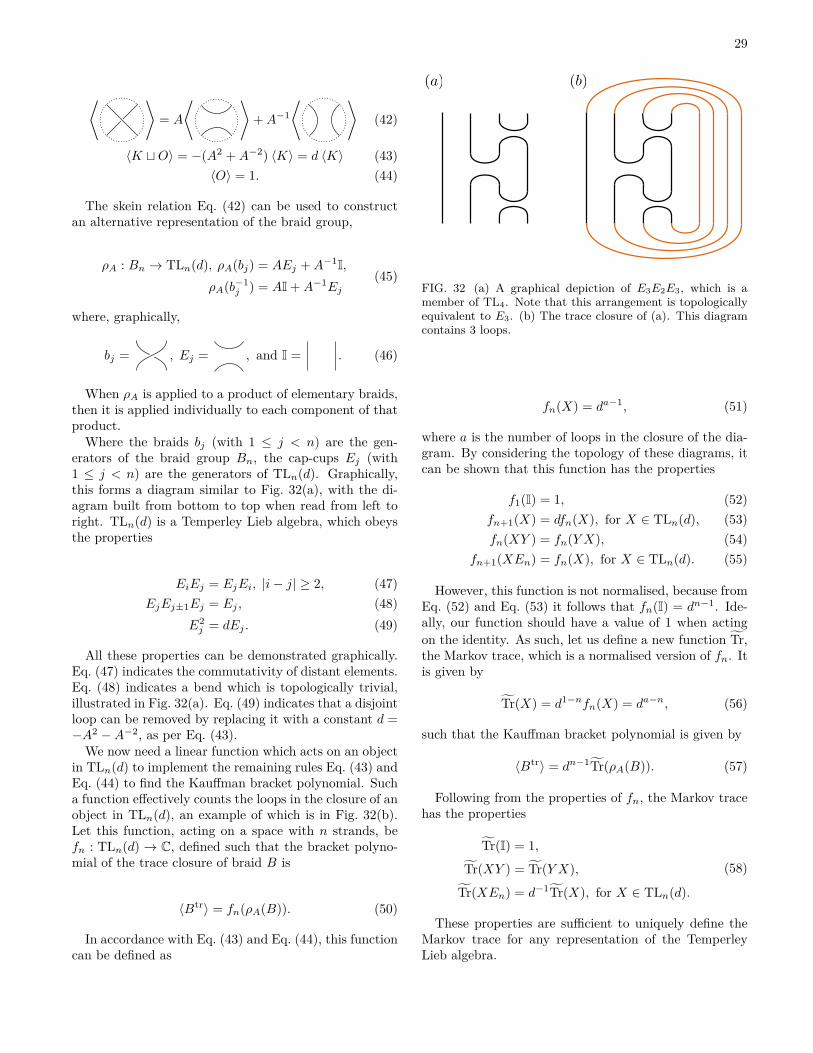
29

⟨ ⟩= A

⟨ ⟩+A−1

⟨ ⟩(42)

〈K tO〉 = −(A2 +A−2) 〈K〉 = d 〈K〉 (43)〈O〉 = 1. (44)

The skein relation Eq. (42) can be used to constructan alternative representation of the braid group,

ρA : Bn → TLn(d), ρA(bj) = AEj +A−1I,ρA(b−1

j ) = AI +A−1Ej(45)

where, graphically,

bj = , Ej = , and I = . (46)

When ρA is applied to a product of elementary braids,then it is applied individually to each component of thatproduct.

Where the braids bj (with 1 ≤ j < n) are the gen-erators of the braid group Bn, the cap-cups Ej (with1 ≤ j < n) are the generators of TLn(d). Graphically,this forms a diagram similar to Fig. 32(a), with the di-agram built from bottom to top when read from left toright. TLn(d) is a Temperley Lieb algebra, which obeysthe properties

EiEj = EjEi, |i− j| ≥ 2, (47)EjEj±1Ej = Ej , (48)

E2j = dEj . (49)

All these properties can be demonstrated graphically.Eq. (47) indicates the commutativity of distant elements.Eq. (48) indicates a bend which is topologically trivial,illustrated in Fig. 32(a). Eq. (49) indicates that a disjointloop can be removed by replacing it with a constant d =−A2 −A−2, as per Eq. (43).We now need a linear function which acts on an object

in TLn(d) to implement the remaining rules Eq. (43) andEq. (44) to find the Kauffman bracket polynomial. Sucha function effectively counts the loops in the closure of anobject in TLn(d), an example of which is in Fig. 32(b).Let this function, acting on a space with n strands, befn : TLn(d) → C, defined such that the bracket polyno-mial of the trace closure of braid B is

〈Btr〉 = fn(ρA(B)). (50)

In accordance with Eq. (43) and Eq. (44), this functioncan be defined as

(a) (b)

FIG. 32 (a) A graphical depiction of E3E2E3, which is amember of TL4. Note that this arrangement is topologicallyequivalent to E3. (b) The trace closure of (a). This diagramcontains 3 loops.

fn(X) = da−1, (51)

where a is the number of loops in the closure of the dia-gram. By considering the topology of these diagrams, itcan be shown that this function has the properties

f1(I) = 1, (52)fn+1(X) = dfn(X), for X ∈ TLn(d), (53)fn(XY ) = fn(Y X), (54)

fn+1(XEn) = fn(X), for X ∈ TLn(d). (55)

However, this function is not normalised, because fromEq. (52) and Eq. (53) it follows that fn(I) = dn−1. Ide-ally, our function should have a value of 1 when actingon the identity. As such, let us define a new function T̃r,the Markov trace, which is a normalised version of fn. Itis given by

T̃r(X) = d1−nfn(X) = da−n, (56)

such that the Kauffman bracket polynomial is given by

〈Btr〉 = dn−1T̃r(ρA(B)). (57)

Following from the properties of fn, the Markov tracehas the properties

T̃r(I) = 1,T̃r(XY ) = T̃r(Y X),

T̃r(XEn) = d−1T̃r(X), for X ∈ TLn(d).

(58)

These properties are sufficient to uniquely define theMarkov trace for any representation of the TemperleyLieb algebra.

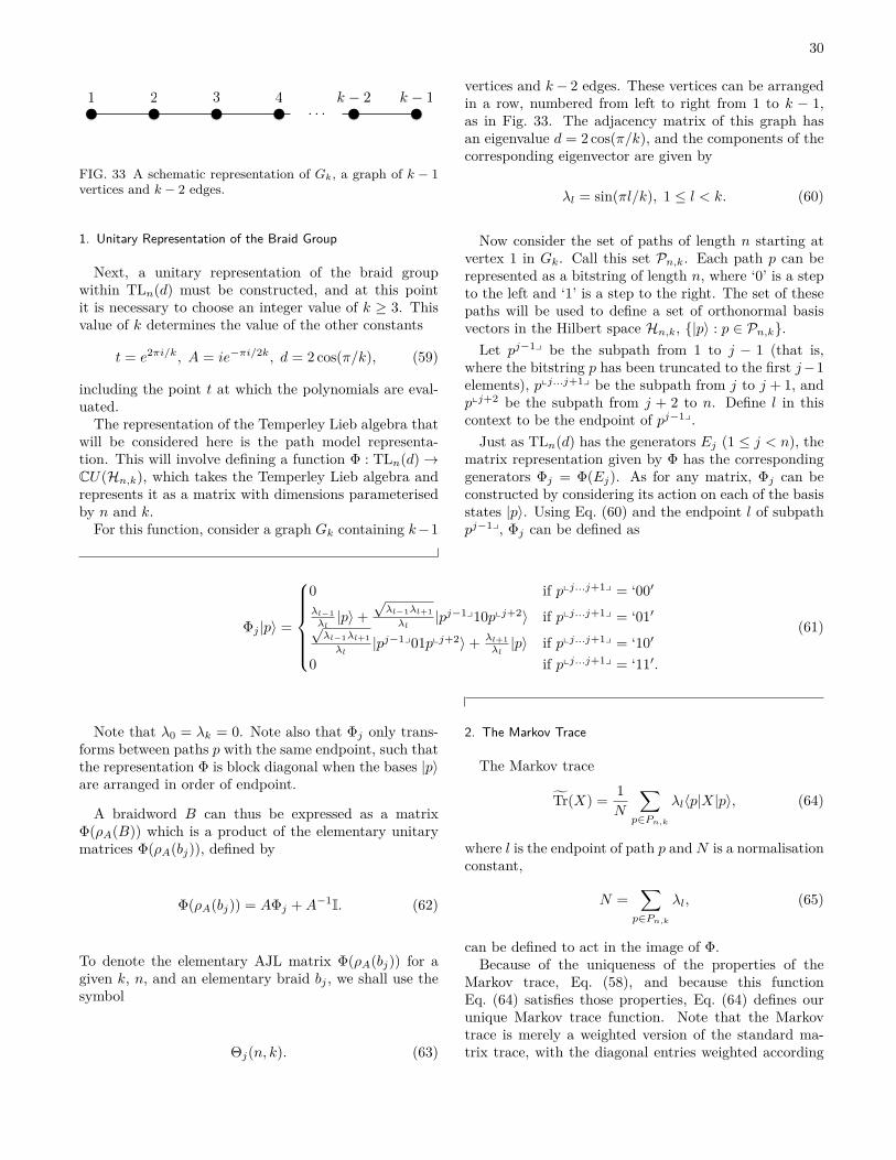
30

. . .k � 2 k � 11 2 3 4

FIG. 33 A schematic representation of Gk, a graph of k − 1vertices and k − 2 edges.

1. Unitary Representation of the Braid Group

Next, a unitary representation of the braid groupwithin TLn(d) must be constructed, and at this pointit is necessary to choose an integer value of k ≥ 3. Thisvalue of k determines the value of the other constants

t = e2πi/k, A = ie−πi/2k, d = 2 cos(π/k), (59)

including the point t at which the polynomials are eval-uated.

The representation of the Temperley Lieb algebra thatwill be considered here is the path model representa-tion. This will involve defining a function Φ : TLn(d)→CU(Hn,k), which takes the Temperley Lieb algebra andrepresents it as a matrix with dimensions parameterisedby n and k.

For this function, consider a graph Gk containing k−1

vertices and k− 2 edges. These vertices can be arrangedin a row, numbered from left to right from 1 to k − 1,as in Fig. 33. The adjacency matrix of this graph hasan eigenvalue d = 2 cos(π/k), and the components of thecorresponding eigenvector are given by

λl = sin(πl/k), 1 ≤ l < k. (60)

Now consider the set of paths of length n starting atvertex 1 in Gk. Call this set Pn,k. Each path p can berepresented as a bitstring of length n, where ‘0’ is a stepto the left and ‘1’ is a step to the right. The set of thesepaths will be used to define a set of orthonormal basisvectors in the Hilbert space Hn,k, {|p〉 : p ∈ Pn,k}.Let pj−1y be the subpath from 1 to j − 1 (that is,

where the bitstring p has been truncated to the first j−1elements), pxj...j+1y be the subpath from j to j + 1, andpxj+2 be the subpath from j + 2 to n. Define l in thiscontext to be the endpoint of pj−1y.Just as TLn(d) has the generators Ej (1 ≤ j < n), the

matrix representation given by Φ has the correspondinggenerators Φj = Φ(Ej). As for any matrix, Φj can beconstructed by considering its action on each of the basisstates |p〉. Using Eq. (60) and the endpoint l of subpathpj−1y, Φj can be defined as

Φj |p〉 =

0 if pxj...j+1y = ‘00′λl−1λl|p〉+

√λl−1λl+1λl

|pj−1y10pxj+2〉 if pxj...j+1y = ‘01′√λl−1λl+1λl

|pj−1y01pxj+2〉+ λl+1λl|p〉 if pxj...j+1y = ‘10′

0 if pxj...j+1y = ‘11′.

(61)

Note that λ0 = λk = 0. Note also that Φj only trans-forms between paths p with the same endpoint, such thatthe representation Φ is block diagonal when the bases |p〉are arranged in order of endpoint.

A braidword B can thus be expressed as a matrixΦ(ρA(B)) which is a product of the elementary unitarymatrices Φ(ρA(bj)), defined by

Φ(ρA(bj)) = AΦj +A−1I. (62)

To denote the elementary AJL matrix Φ(ρA(bj)) for agiven k, n, and an elementary braid bj , we shall use thesymbol

Θj(n, k). (63)

2. The Markov Trace

The Markov trace

T̃r(X) = 1N

∑p∈Pn,k

λl〈p|X|p〉, (64)

where l is the endpoint of path p andN is a normalisationconstant,

N =∑

p∈Pn,k

λl, (65)

can be defined to act in the image of Φ.Because of the uniqueness of the properties of the

Markov trace, Eq. (58), and because this functionEq. (64) satisfies those properties, Eq. (64) defines ourunique Markov trace function. Note that the Markovtrace is merely a weighted version of the standard ma-trix trace, with the diagonal entries weighted according

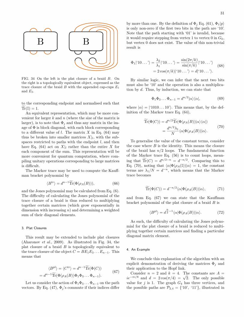
31

BB

FIG. 34 On the left is the plat closure of a braid B. Onthe right is a topologically equivalent object, expressed as thetrace closure of the braid B with the appended cap-cups E1and E3.

to the corresponding endpoint and normalised such thatT̃r(I) = 1.An equivalent representation, which may be more con-

venient for larger k and n (where the size of the matrix islarger), is to note that Φj and thus any matrix in the im-age of Φ is block diagonal, with each block correspondingto a different value of l. The matrix X in Eq. (64) maythus be broken into smaller matrices X|l, with the sub-spaces restricted to paths with the endpoint l, and thenhave Eq. (64) act on X|l rather than the entire X foreach component of the sum. This representation will bemore convenient for quantum computation, where com-piling unitary operations corresponding to large matricesis difficult.

The Markov trace may be used to compute the Kauff-man bracket polynomial by

〈Btr〉 = dn−1T̃r(Φ(ρA(B))), (66)

and the Jones polynomial may be calculated from Eq. (6).The difficulty of calculating the Jones polynomial of thetrace closure of a braid is thus reduced to multiplyingtogether certain matrices (which grow exponentially indimension with increasing n) and determining a weightedsum of their diagonal elements.

3. Plat Closures

This result may be extended to include plat closures(Aharonov et al., 2009). As illustrated in Fig. 34, theplat closure of a braid B is topologically equivalent tothe trace closure of the object C = BE1E3 . . . En−1. Thismeans that

〈Bpl〉 = 〈Ctr〉 = dn−1T̃r(Φ(C))= dn−1T̃r(Φ(ρA(B))Φ1Φ3 . . .Φn−1).

(67)

Let us consider the action of Φ1Φ3 . . .Φn−1 on the pathvectors. By Eq. (47), Φj ’s commute if their indices differ

by more than one. By the definition of Φj Eq. (61), Φ1|p〉is only non-zero if the first two bits in the path are ‘10’.Note that the path starting with ‘01’ is invalid, becauseit would require stepping from vertex 1 to vertex 0 in Gk,but vertex 0 does not exist. The value of this non-trivialresult is

Φ1|‘10 . . . ’〉 = λ2λ1|‘10 . . . ’〉 = sin(2π/k)

sin(π/k) |‘10 . . . ’〉

= 2 cos(π/k)|‘10 . . . ’〉 = d|‘10 . . . ’〉.(68)

By similar logic, we can infer that the next two bitsmust also be ‘10’ and the operation is also a multiplica-tion by d. Thus, by induction, we can state that

Φ1Φ3 . . .Φn−1 = dn/2|α〉〈α|, (69)

where |α〉 = |‘1010 . . . 10’〉. This means that, by the def-inition of the Markov trace Eq. (64),

T̃r(Φ(C)) = dn/2T̃r(Φ(ρA(B))|α〉〈α|)

= dn/2λ1N

〈α|Φ(ρA(B))|α〉.(70)

To generalise the value of the constant terms, considerthe case where B is the identity. This means the closureof the braid has n/2 loops. The fundamental functionof the Markov trace Eq. (56) is to count loops, mean-ing that T̃r(C) = dn/2−n = d−n/2. Comparing this toEq. (70), noting that 〈α|Φ(ρA(I))|α〉 = 1, the constantterms are λ1/N = d−n, which means that the Markovtrace becomes

T̃r(Φ(C)) = d−n/2〈α|Φ(ρA(B))|α〉, (71)

and from Eq. (67) we can state that the Kauffmanbracket polynomial of the plat closure of a braid B is

〈Bpl〉 = dn2−1〈α|Φ(ρA(B))|α〉. (72)

As such, the difficulty of calculating the Jones polyno-mial for the plat closure of a braid is reduced to multi-plying together certain matrices and finding a particulardiagonal matrix element.

4. An Example

We conclude this explanation of the algorithm with anexplicit demonstration of deriving the matrices Φj andtheir application to the Hopf link.Consider n = 2 and k = 4. The constants are A =

ie−πi/8 and d = 2 cos(π/4) =√

2. The only possiblevalue for j is 1. The graph G4 has three vertices, andthe possible paths are P2,4 = {‘10’, ‘11’}, illustrated in

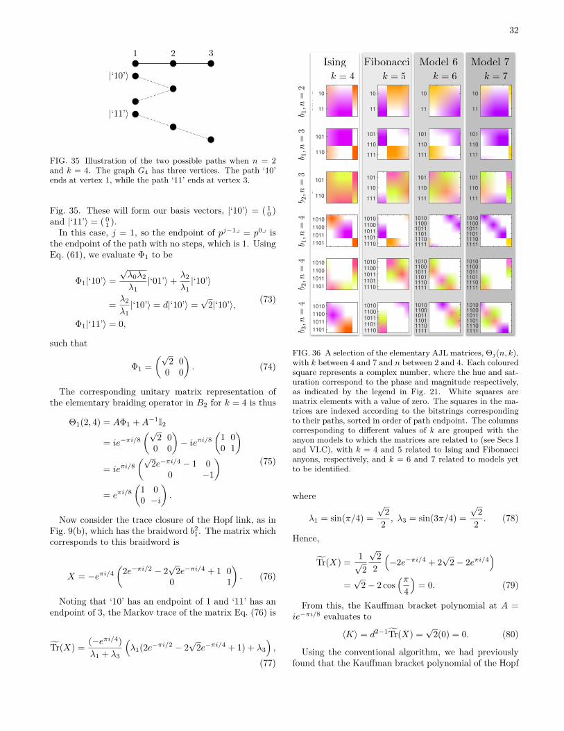
32

1 2 3

|‘10’i

|‘11’i

FIG. 35 Illustration of the two possible paths when n = 2and k = 4. The graph G4 has three vertices. The path ‘10’ends at vertex 1, while the path ‘11’ ends at vertex 3.

Fig. 35. These will form our basis vectors, |‘10’〉 = ( 10 )

and |‘11’〉 = ( 01 ).

In this case, j = 1, so the endpoint of pj−1y = p0y isthe endpoint of the path with no steps, which is 1. UsingEq. (61), we evaluate Φ1 to be

Φ1|‘10’〉 =√λ0λ2λ1

|‘01’〉+ λ2λ1|‘10’〉

= λ2λ1|‘10’〉 = d|‘10’〉 =

√2|‘10’〉,

Φ1|‘11’〉 = 0,

(73)

such that

Φ1 =(√

2 00 0

). (74)

The corresponding unitary matrix representation ofthe elementary braiding operator in B2 for k = 4 is thus

Θ1(2, 4) = AΦ1 +A−1I2

= ie−πi/8(√

2 00 0

)− ieπi/8

(1 00 1

)= ieπi/8

(√2e−πi/4 − 1 0

0 −1

)= eπi/8

(1 00 −i

).

(75)

Now consider the trace closure of the Hopf link, as inFig. 9(b), which has the braidword b2

1. The matrix whichcorresponds to this braidword is

X = −eπi/4(

2e−πi/2 − 2√

2e−πi/4 + 1 00 1

). (76)

Noting that ‘10’ has an endpoint of 1 and ‘11’ has anendpoint of 3, the Markov trace of the matrix Eq. (76) is

T̃r(X) = (−eπi/4)λ1 + λ3

(λ1(2e−πi/2 − 2

√2e−πi/4 + 1) + λ3

),

(77)

k=4

10

11b1, n=

2

k=5

10

11

k=6

10

11

k=7

10

11

101

110b1, n=

3

101

110b2, n=

3

101

110

111

101

110

111

101

110

111

101

110

111

101

110

111

101

110

111

1010

1100

1011

1101

b1, n=

4

1010

1100

1011

1101

b2, n=

41010

1100

1011

1101

b3, n=

4

10101100101111011110

10101100101111011110

10101100101111011110

101011001011110111101111

101011001011110111101111

101011001011110111101111

101011001011110111101111

101011001011110111101111

101011001011110111101111

k = 4 k = 5 k = 6 k = 7

b 1,n

=3

b 2,n

=3

b 1,n

=4

b 2,n

=4

b 3,n

=4

b 1,n

=2

FibonacciIsing Model 6 Model 7

FIG. 36 A selection of the elementary AJL matrices, Θj(n, k),with k between 4 and 7 and n between 2 and 4. Each colouredsquare represents a complex number, where the hue and sat-uration correspond to the phase and magnitude respectively,as indicated by the legend in Fig. 21. White squares arematrix elements with a value of zero. The squares in the ma-trices are indexed according to the bitstrings correspondingto their paths, sorted in order of path endpoint. The columnscorresponding to different values of k are grouped with theanyon models to which the matrices are related to (see Secs Iand VI.C), with k = 4 and 5 related to Ising and Fibonaccianyons, respectively, and k = 6 and 7 related to models yetto be identified.

where

λ1 = sin(π/4) =√

22 , λ3 = sin(3π/4) =

√2

2 . (78)

Hence,

T̃r(X) = 1√2

√2

2

(−2e−πi/4 + 2

√2− 2eπi/4

)=√

2− 2 cos(π

4

)= 0. (79)

From this, the Kauffman bracket polynomial at A =ie−πi/8 evaluates to

〈K〉 = d2−1T̃r(X) =√

2(0) = 0. (80)

Using the conventional algorithm, we had previouslyfound that the Kauffman bracket polynomial of the Hopf

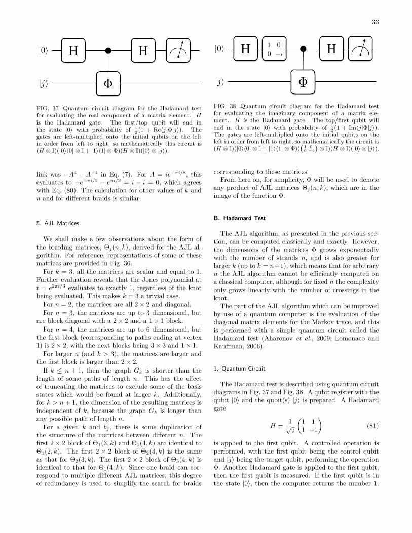
33

|0i

|ji

HH

�

FIG. 37 Quantum circuit diagram for the Hadamard testfor evaluating the real component of a matrix element. His the Hadamard gate. The first/top qubit will end inthe state |0〉 with probability of 1

2 (1 + Re〈j|Φ|j〉). Thegates are left-multiplied onto the initial qubits on the leftin order from left to right, so mathematically this circuit is(H ⊗ I)(|0〉〈0| ⊗ I + |1〉〈1| ⊗ Φ)(H ⊗ I)(|0〉 ⊗ |j〉).

link was −A4 − A−4 in Eq. (7). For A = ie−πi/8, thisevaluates to −e−πi/2 − eπi/2 = i − i = 0, which agreeswith Eq. (80). The calculation for other values of k andn and for different braids is similar.

5. AJL Matrices

We shall make a few observations about the form ofthe braiding matrices, Θj(n, k), derived for the AJL al-gorithm. For reference, representations of some of thesematrices are provided in Fig. 36.

For k = 3, all the matrices are scalar and equal to 1.Further evaluation reveals that the Jones polynomial att = e2πi/3 evaluates to exactly 1, regardless of the knotbeing evaluated. This makes k = 3 a trivial case.For n = 2, the matrices are all 2× 2 and diagonal.For n = 3, the matrices are up to 3 dimensional, but

are block diagonal with a 2× 2 and a 1× 1 block.For n = 4, the matrices are up to 6 dimensional, but

the first block (corresponding to paths ending at vertex1) is 2× 2, with the next blocks being 3× 3 and 1× 1.

For larger n (and k > 3), the matrices are larger andthe first block is larger than 2× 2.

If k ≤ n + 1, then the graph Gk is shorter than thelength of some paths of length n. This has the effectof truncating the matrices to exclude some of the basisstates which would be found at larger k. Additionally,for k > n+ 1, the dimension of the resulting matrices isindependent of k, because the graph Gk is longer thanany possible path of length n.For a given k and bj , there is some duplication of

the structure of the matrices between different n. Thefirst 2× 2 block of Θ1(3, k) and Θ1(4, k) are identical toΘ1(2, k). The first 2 × 2 block of Θ2(4, k) is the sameas that for Θ2(3, k). The first 2 × 2 block of Θ3(4, k) isidentical to that for Θ1(4, k). Since one braid can cor-respond to multiple different AJL matrices, this degreeof redundancy is used to simplify the search for braids

|0i

|ji

H

�

01

�i

0H

FIG. 38 Quantum circuit diagram for the Hadamard testfor evaluating the imaginary component of a matrix ele-ment. H is the Hadamard gate. The top/first qubit willend in the state |0〉 with probability of 1

2 (1 + Im〈j|Φ|j〉).The gates are left-multiplied onto the initial qubits on theleft in order from left to right, so mathematically the circuit is(H ⊗ I)(|0〉〈0| ⊗ I + |1〉〈1| ⊗ Φ)(

(1 00 −i

)⊗ I)(H ⊗ I)(|0〉 ⊗ |j〉).

corresponding to these matrices.From here on, for simplicity, Φ will be used to denote

any product of AJL matrices Θj(n, k), which are in theimage of the function Φ.

B. Hadamard Test

The AJL algorithm, as presented in the previous sec-tion, can be computed classically and exactly. However,the dimensions of the matrices Φ grows exponentiallywith the number of strands n, and is also greater forlarger k (up to k = n+1), which means that for arbitraryn the AJL algorithm cannot be efficiently computed ona classical computer, although for fixed n the complexityonly grows linearly with the number of crossings in theknot.

The part of the AJL algorithm which can be improvedby use of a quantum computer is the evaluation of thediagonal matrix elements for the Markov trace, and thisis performed with a simple quantum circuit called theHadamard test (Aharonov et al., 2009; Lomonaco andKauffman, 2006).

1. Quantum Circuit

The Hadamard test is described using quantum circuitdiagrams in Fig. 37 and Fig. 38. A qubit register with thequbit |0〉 and the qubit(s) |j〉 is prepared. A Hadamardgate

H = 1√2

(1 11 −1

)(81)

is applied to the first qubit. A controlled operation isperformed, with the first qubit being the control qubitand |j〉 being the target qubit, performing the operationΦ. Another Hadamard gate is applied to the first qubit,then the first qubit is measured. If the first qubit is inthe state |0〉, then the computer returns the number 1.

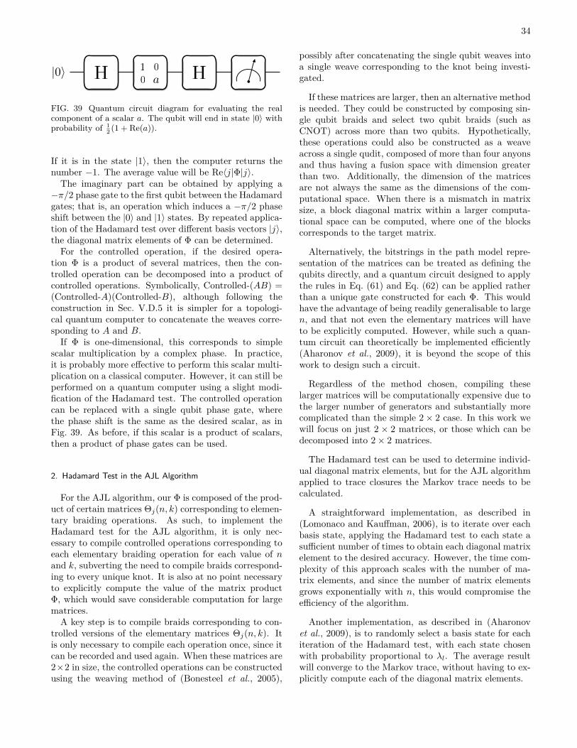
34

|0i HH 01 0

a

FIG. 39 Quantum circuit diagram for evaluating the realcomponent of a scalar a. The qubit will end in state |0〉 withprobability of 1

2 (1 + Re(a)).

If it is in the state |1〉, then the computer returns thenumber −1. The average value will be Re〈j|Φ|j〉.

The imaginary part can be obtained by applying a−π/2 phase gate to the first qubit between the Hadamardgates; that is, an operation which induces a −π/2 phaseshift between the |0〉 and |1〉 states. By repeated applica-tion of the Hadamard test over different basis vectors |j〉,the diagonal matrix elements of Φ can be determined.For the controlled operation, if the desired opera-

tion Φ is a product of several matrices, then the con-trolled operation can be decomposed into a product ofcontrolled operations. Symbolically, Controlled-(AB) =(Controlled-A)(Controlled-B), although following theconstruction in Sec. V.D.5 it is simpler for a topologi-cal quantum computer to concatenate the weaves corre-sponding to A and B.If Φ is one-dimensional, this corresponds to simple

scalar multiplication by a complex phase. In practice,it is probably more effective to perform this scalar multi-plication on a classical computer. However, it can still beperformed on a quantum computer using a slight modi-fication of the Hadamard test. The controlled operationcan be replaced with a single qubit phase gate, wherethe phase shift is the same as the desired scalar, as inFig. 39. As before, if this scalar is a product of scalars,then a product of phase gates can be used.

2. Hadamard Test in the AJL Algorithm

For the AJL algorithm, our Φ is composed of the prod-uct of certain matrices Θj(n, k) corresponding to elemen-tary braiding operations. As such, to implement theHadamard test for the AJL algorithm, it is only nec-essary to compile controlled operations corresponding toeach elementary braiding operation for each value of nand k, subverting the need to compile braids correspond-ing to every unique knot. It is also at no point necessaryto explicitly compute the value of the matrix productΦ, which would save considerable computation for largematrices.

A key step is to compile braids corresponding to con-trolled versions of the elementary matrices Θj(n, k). Itis only necessary to compile each operation once, since itcan be recorded and used again. When these matrices are2×2 in size, the controlled operations can be constructedusing the weaving method of (Bonesteel et al., 2005),

possibly after concatenating the single qubit weaves intoa single weave corresponding to the knot being investi-gated.

If these matrices are larger, then an alternative methodis needed. They could be constructed by composing sin-gle qubit braids and select two qubit braids (such asCNOT) across more than two qubits. Hypothetically,these operations could also be constructed as a weaveacross a single qudit, composed of more than four anyonsand thus having a fusion space with dimension greaterthan two. Additionally, the dimension of the matricesare not always the same as the dimensions of the com-putational space. When there is a mismatch in matrixsize, a block diagonal matrix within a larger computa-tional space can be computed, where one of the blockscorresponds to the target matrix.

Alternatively, the bitstrings in the path model repre-sentation of the matrices can be treated as defining thequbits directly, and a quantum circuit designed to applythe rules in Eq. (61) and Eq. (62) can be applied ratherthan a unique gate constructed for each Φ. This wouldhave the advantage of being readily generalisable to largen, and that not even the elementary matrices will haveto be explicitly computed. However, while such a quan-tum circuit can theoretically be implemented efficiently(Aharonov et al., 2009), it is beyond the scope of thiswork to design such a circuit.

Regardless of the method chosen, compiling theselarger matrices will be computationally expensive due tothe larger number of generators and substantially morecomplicated than the simple 2× 2 case. In this work wewill focus on just 2 × 2 matrices, or those which can bedecomposed into 2× 2 matrices.

The Hadamard test can be used to determine individ-ual diagonal matrix elements, but for the AJL algorithmapplied to trace closures the Markov trace needs to becalculated.

A straightforward implementation, as described in(Lomonaco and Kauffman, 2006), is to iterate over eachbasis state, applying the Hadamard test to each state asufficient number of times to obtain each diagonal matrixelement to the desired accuracy. However, the time com-plexity of this approach scales with the number of ma-trix elements, and since the number of matrix elementsgrows exponentially with n, this would compromise theefficiency of the algorithm.

Another implementation, as described in (Aharonovet al., 2009), is to randomly select a basis state for eachiteration of the Hadamard test, with each state chosenwith probability proportional to λl. The average resultwill converge to the Markov trace, without having to ex-plicitly compute each of the diagonal matrix elements.

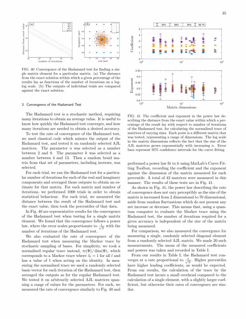
35

0 0.2 0.4 0.6 0.8

−0.8

−0.6

−0.4

−0.2

0

exact

101 102 103 104 105

10−2

10−1

100

50% 68% 95%99.7%

imagin

ary

part

real partnumber of iterations

dis

tance

from

exact

valu

e 101

102

103

104

105

106

(a) (b)

FIG. 40 Convergence of the Hadamard test for finding a sin-gle matrix element for a particular matrix. (a) The distancefrom the exact solution within which a given percentage of theresults lay as functions of the number of iterations on a log-log scale. (b) The outputs of individual trials are comparedagainst the exact solution.

3. Convergence of the Hadamard Test

The Hadamard test is a stochastic method, requiringmany iterations to obtain an average value. It is useful toknow how quickly the Hadamard test converges, and howmany iterations are needed to obtain a desired accuracy.

To test the rate of convergence of the Hadamard test,we used classical code which mimics the output of theHadamard test, and tested it on randomly selected AJLmatrices. The parameter n was selected as a numberbetween 2 and 8. The parameter k was selected as anumber between 4 and 13. Then a random braid ma-trix from that set of parameters, including inverses, wasselected.

For each trial, we ran the Hadamard test for a particu-lar number of iterations for each of the real and imaginarycomponents and averaged those outputs to obtain an es-timate for that matrix. For each matrix and number ofiterations, we performed 1000 trials in order to obtainstatistical behaviour. For each trial, we measured thedistance between the result of the Hadamard test andthe exact value, then took the percentiles of that data.

In Fig. 40 are representative results for the convergenceof the Hadamard test when testing for a single matrixelement. We found that the convergence follows a powerlaw, where the error scales proportionate to 1√

Nwith the

number of iterations of the Hadamard test.We also evaluated the rate of convergence of the

Hadamard test when measuring the Markov trace bystochastic sampling of bases. For simplicity, we took anormalised regular trace instead, tr(Φ)/ dim(Φ), whichcorresponds to a Markov trace where λl = 1 for all l andhas a value of 1 when acting on the identity. In mea-suring the normalised trace we used a randomly selectedbasis vector for each iteration of the Hadamard test, thenaveraged the outputs as for the regular Hadamard test.We tested it on arbitrarily selected AJL matrices span-ning a range of values for the parameters. For each, wemeasured the rate of convergence similarly to Fig. 40 and

100

101

102

0

1

2

3

4

5

Co

eff

icie

nt

50% 68% 95% 99.7%

100

101

102

Matrix dimensions

-0.6

-0.55

-0.5

-0.45

-0.4

-0.35

Po

we

rE

xpon

ent

Coe�

cien

t

Matrix dimensions

FIG. 41 The coefficient and exponent in the power law de-scribing the distance from the exact value within which a per-centage of the result lay with respect to number of iterationsof the Hadamard test, for calculating the normalised trace ofmatrices of varying sizes. Each point is a different matrix thatwas tested, representing a range of dimensions. The log scalein the matrix dimensions reflects the fact that the size of theAJL matrices grows exponentially with increasing n. Errorbars represent 95% confidence intervals for the curve fitting.

performed a power law fit to it using MatLab’s Curve Fit-ting Toolbox, recording the coefficient and the exponentagainst the dimension of the matrix measured for eachpercentile. A total of 42 matrices were measured in thismanner. The results of these tests are in Fig. 41.As shown in Fig. 41, the power law describing the rate

of convergence does not vary perceptibly as the size of thematrix is increased from 2 dimensional to 70 dimensional,aside from random fluctuations which do not present anynet increase or decrease. This means that, using a quan-tum computer to evaluate the Markov trace using theHadamard test, the number of iterations required for agiven accuracy is independent of the size of the matrixbeing measured.For comparison, we also measured the convergence for

measuring a single, randomly selected diagonal elementfrom a randomly selected AJL matrix. We made 20 suchmeasurements. The mean of the measured coefficientsand powers was taken and recorded in Table I.From our results in Table I, the Hadamard test con-

verges at a rate proportional to 1√N. Higher percentiles

have higher leading coefficients, as would be expected.From our results, the calculation of the trace by theHadamard test incurs a small overhead compared to thecalculation of a single element, with a slightly larger coef-ficient, but otherwise their rates of convergence are sim-ilar.

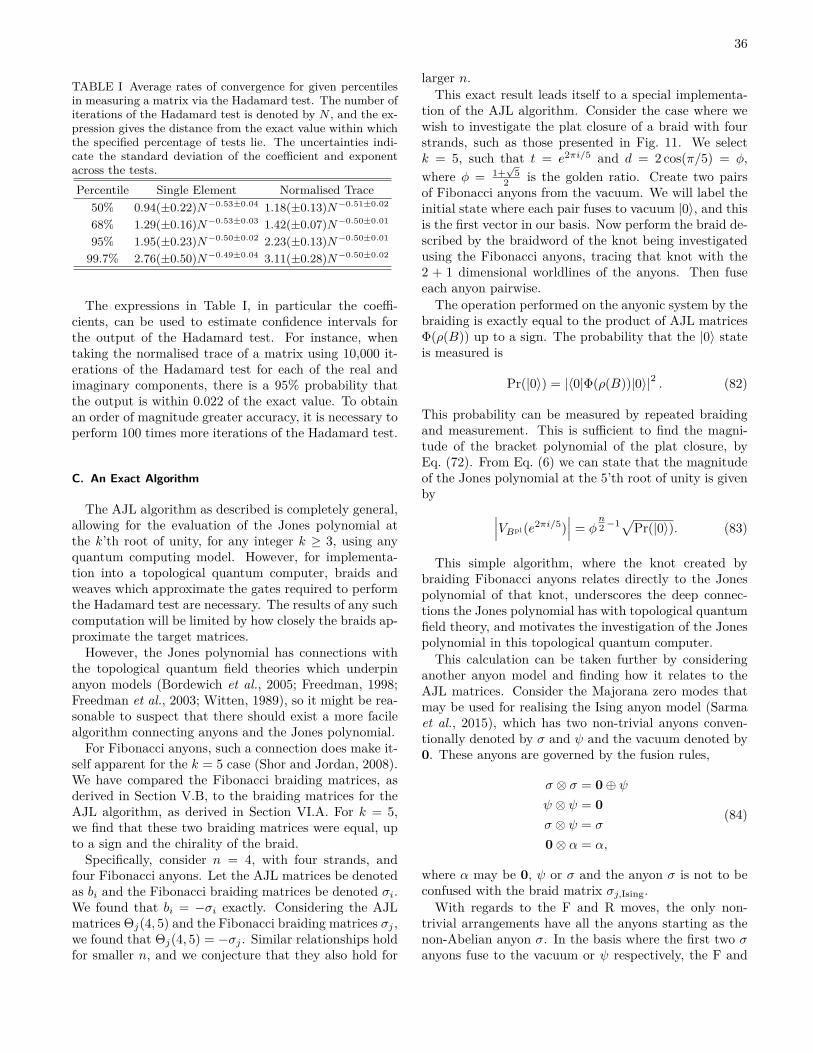
36

TABLE I Average rates of convergence for given percentilesin measuring a matrix via the Hadamard test. The number ofiterations of the Hadamard test is denoted by N , and the ex-pression gives the distance from the exact value within whichthe specified percentage of tests lie. The uncertainties indi-cate the standard deviation of the coefficient and exponentacross the tests.Percentile Single Element Normalised Trace

50% 0.94(±0.22)N−0.53±0.04 1.18(±0.13)N−0.51±0.02

68% 1.29(±0.16)N−0.53±0.03 1.42(±0.07)N−0.50±0.01

95% 1.95(±0.23)N−0.50±0.02 2.23(±0.13)N−0.50±0.01

99.7% 2.76(±0.50)N−0.49±0.04 3.11(±0.28)N−0.50±0.02

The expressions in Table I, in particular the coeffi-cients, can be used to estimate confidence intervals forthe output of the Hadamard test. For instance, whentaking the normalised trace of a matrix using 10,000 it-erations of the Hadamard test for each of the real andimaginary components, there is a 95% probability thatthe output is within 0.022 of the exact value. To obtainan order of magnitude greater accuracy, it is necessary toperform 100 times more iterations of the Hadamard test.

C. An Exact Algorithm

The AJL algorithm as described is completely general,allowing for the evaluation of the Jones polynomial atthe k’th root of unity, for any integer k ≥ 3, using anyquantum computing model. However, for implementa-tion into a topological quantum computer, braids andweaves which approximate the gates required to performthe Hadamard test are necessary. The results of any suchcomputation will be limited by how closely the braids ap-proximate the target matrices.

However, the Jones polynomial has connections withthe topological quantum field theories which underpinanyon models (Bordewich et al., 2005; Freedman, 1998;Freedman et al., 2003; Witten, 1989), so it might be rea-sonable to suspect that there should exist a more facilealgorithm connecting anyons and the Jones polynomial.

For Fibonacci anyons, such a connection does make it-self apparent for the k = 5 case (Shor and Jordan, 2008).We have compared the Fibonacci braiding matrices, asderived in Section V.B, to the braiding matrices for theAJL algorithm, as derived in Section VI.A. For k = 5,we find that these two braiding matrices were equal, upto a sign and the chirality of the braid.

Specifically, consider n = 4, with four strands, andfour Fibonacci anyons. Let the AJL matrices be denotedas bi and the Fibonacci braiding matrices be denoted σi.We found that bi = −σi exactly. Considering the AJLmatrices Θj(4, 5) and the Fibonacci braiding matrices σj ,we found that Θj(4, 5) = −σj . Similar relationships holdfor smaller n, and we conjecture that they also hold for

larger n.This exact result leads itself to a special implementa-

tion of the AJL algorithm. Consider the case where wewish to investigate the plat closure of a braid with fourstrands, such as those presented in Fig. 11. We selectk = 5, such that t = e2πi/5 and d = 2 cos(π/5) = φ,where φ = 1+

√5

2 is the golden ratio. Create two pairsof Fibonacci anyons from the vacuum. We will label theinitial state where each pair fuses to vacuum |0〉, and thisis the first vector in our basis. Now perform the braid de-scribed by the braidword of the knot being investigatedusing the Fibonacci anyons, tracing that knot with the2 + 1 dimensional worldlines of the anyons. Then fuseeach anyon pairwise.The operation performed on the anyonic system by the

braiding is exactly equal to the product of AJL matricesΦ(ρ(B)) up to a sign. The probability that the |0〉 stateis measured is

Pr(|0〉) = |〈0|Φ(ρ(B))|0〉|2 . (82)

This probability can be measured by repeated braidingand measurement. This is sufficient to find the magni-tude of the bracket polynomial of the plat closure, byEq. (72). From Eq. (6) we can state that the magnitudeof the Jones polynomial at the 5’th root of unity is givenby ∣∣∣VBpl(e2πi/5)

∣∣∣ = φn2−1√Pr(|0〉). (83)

This simple algorithm, where the knot created bybraiding Fibonacci anyons relates directly to the Jonespolynomial of that knot, underscores the deep connec-tions the Jones polynomial has with topological quantumfield theory, and motivates the investigation of the Jonespolynomial in this topological quantum computer.This calculation can be taken further by considering

another anyon model and finding how it relates to theAJL matrices. Consider the Majorana zero modes thatmay be used for realising the Ising anyon model (Sarmaet al., 2015), which has two non-trivial anyons conven-tionally denoted by σ and ψ and the vacuum denoted by0. These anyons are governed by the fusion rules,

σ ⊗ σ = 0⊕ ψψ ⊗ ψ = 0σ ⊗ ψ = σ

0⊗ α = α,

(84)

where α may be 0, ψ or σ and the anyon σ is not to beconfused with the braid matrix σj,Ising.With regards to the F and R moves, the only non-

trivial arrangements have all the anyons starting as thenon-Abelian anyon σ. In the basis where the first two σanyons fuse to the vacuum or ψ respectively, the F and

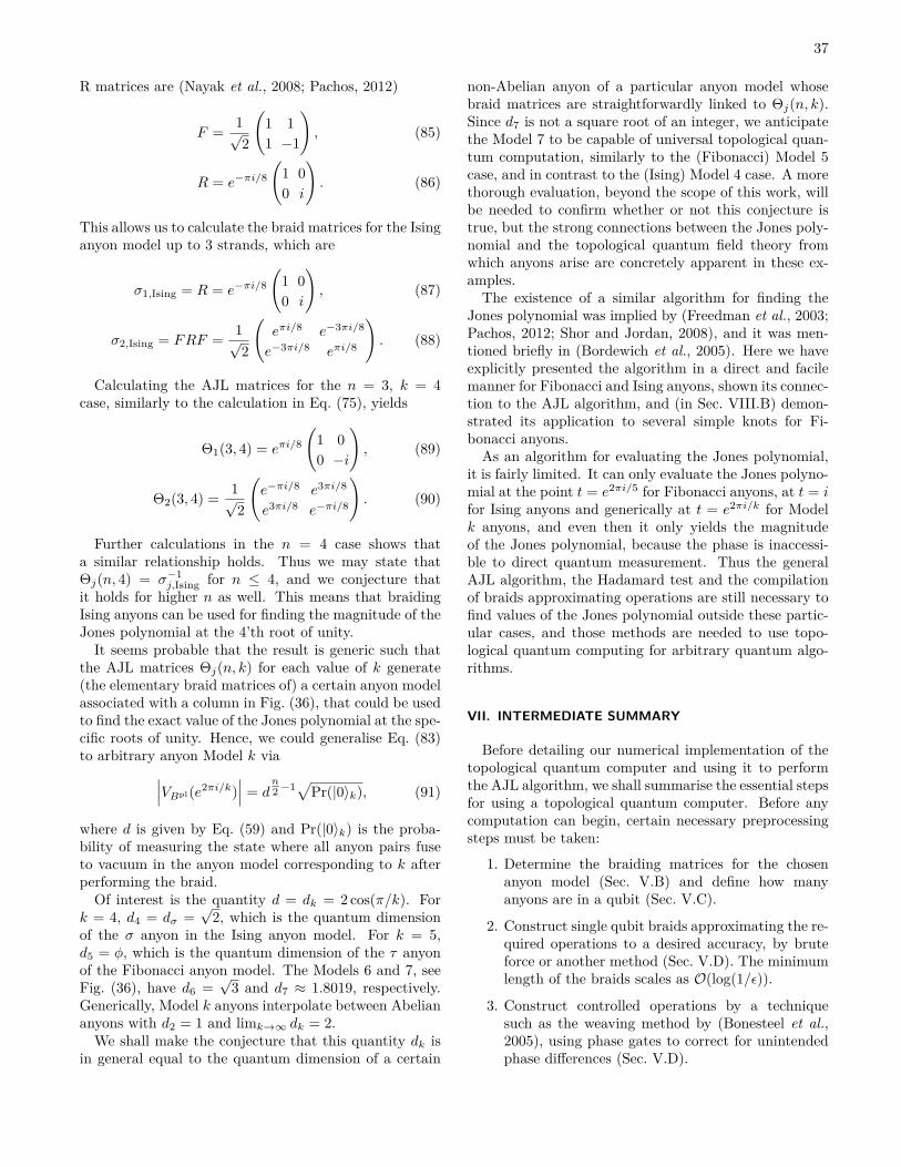
37

R matrices are (Nayak et al., 2008; Pachos, 2012)

F = 1√2

(1 11 −1

), (85)

R = e−πi/8

(1 00 i

). (86)

This allows us to calculate the braid matrices for the Isinganyon model up to 3 strands, which are

σ1,Ising = R = e−πi/8

(1 00 i

), (87)

σ2,Ising = FRF = 1√2

(eπi/8 e−3πi/8

e−3πi/8 eπi/8

). (88)

Calculating the AJL matrices for the n = 3, k = 4case, similarly to the calculation in Eq. (75), yields

Θ1(3, 4) = eπi/8

(1 00 −i

), (89)

Θ2(3, 4) = 1√2

(e−πi/8 e3πi/8

e3πi/8 e−πi/8

). (90)

Further calculations in the n = 4 case shows thata similar relationship holds. Thus we may state thatΘj(n, 4) = σ−1

j,Ising for n ≤ 4, and we conjecture thatit holds for higher n as well. This means that braidingIsing anyons can be used for finding the magnitude of theJones polynomial at the 4’th root of unity.

It seems probable that the result is generic such thatthe AJL matrices Θj(n, k) for each value of k generate(the elementary braid matrices of) a certain anyon modelassociated with a column in Fig. (36), that could be usedto find the exact value of the Jones polynomial at the spe-cific roots of unity. Hence, we could generalise Eq. (83)to arbitrary anyon Model k via∣∣∣VBpl(e2πi/k)

∣∣∣ = dn2−1√Pr(|0〉k), (91)

where d is given by Eq. (59) and Pr(|0〉k) is the proba-bility of measuring the state where all anyon pairs fuseto vacuum in the anyon model corresponding to k afterperforming the braid.

Of interest is the quantity d = dk = 2 cos(π/k). Fork = 4, d4 = dσ =

√2, which is the quantum dimension

of the σ anyon in the Ising anyon model. For k = 5,d5 = φ, which is the quantum dimension of the τ anyonof the Fibonacci anyon model. The Models 6 and 7, seeFig. (36), have d6 =

√3 and d7 ≈ 1.8019, respectively.

Generically, Model k anyons interpolate between Abeliananyons with d2 = 1 and limk→∞ dk = 2.We shall make the conjecture that this quantity dk is

in general equal to the quantum dimension of a certain

non-Abelian anyon of a particular anyon model whosebraid matrices are straightforwardly linked to Θj(n, k).Since d7 is not a square root of an integer, we anticipatethe Model 7 to be capable of universal topological quan-tum computation, similarly to the (Fibonacci) Model 5case, and in contrast to the (Ising) Model 4 case. A morethorough evaluation, beyond the scope of this work, willbe needed to confirm whether or not this conjecture istrue, but the strong connections between the Jones poly-nomial and the topological quantum field theory fromwhich anyons arise are concretely apparent in these ex-amples.The existence of a similar algorithm for finding the

Jones polynomial was implied by (Freedman et al., 2003;Pachos, 2012; Shor and Jordan, 2008), and it was men-tioned briefly in (Bordewich et al., 2005). Here we haveexplicitly presented the algorithm in a direct and facilemanner for Fibonacci and Ising anyons, shown its connec-tion to the AJL algorithm, and (in Sec. VIII.B) demon-strated its application to several simple knots for Fi-bonacci anyons.As an algorithm for evaluating the Jones polynomial,

it is fairly limited. It can only evaluate the Jones polyno-mial at the point t = e2πi/5 for Fibonacci anyons, at t = ifor Ising anyons and generically at t = e2πi/k for Modelk anyons, and even then it only yields the magnitudeof the Jones polynomial, because the phase is inaccessi-ble to direct quantum measurement. Thus the generalAJL algorithm, the Hadamard test and the compilationof braids approximating operations are still necessary tofind values of the Jones polynomial outside these partic-ular cases, and those methods are needed to use topo-logical quantum computing for arbitrary quantum algo-rithms.

VII. INTERMEDIATE SUMMARY

Before detailing our numerical implementation of thetopological quantum computer and using it to performthe AJL algorithm, we shall summarise the essential stepsfor using a topological quantum computer. Before anycomputation can begin, certain necessary preprocessingsteps must be taken:

1. Determine the braiding matrices for the chosenanyon model (Sec. V.B) and define how manyanyons are in a qubit (Sec. V.C).

2. Construct single qubit braids approximating the re-quired operations to a desired accuracy, by bruteforce or another method (Sec. V.D). The minimumlength of the braids scales as O(log(1/ε)).

3. Construct controlled operations by a techniquesuch as the weaving method by (Bonesteel et al.,2005), using phase gates to correct for unintendedphase differences (Sec. V.D).

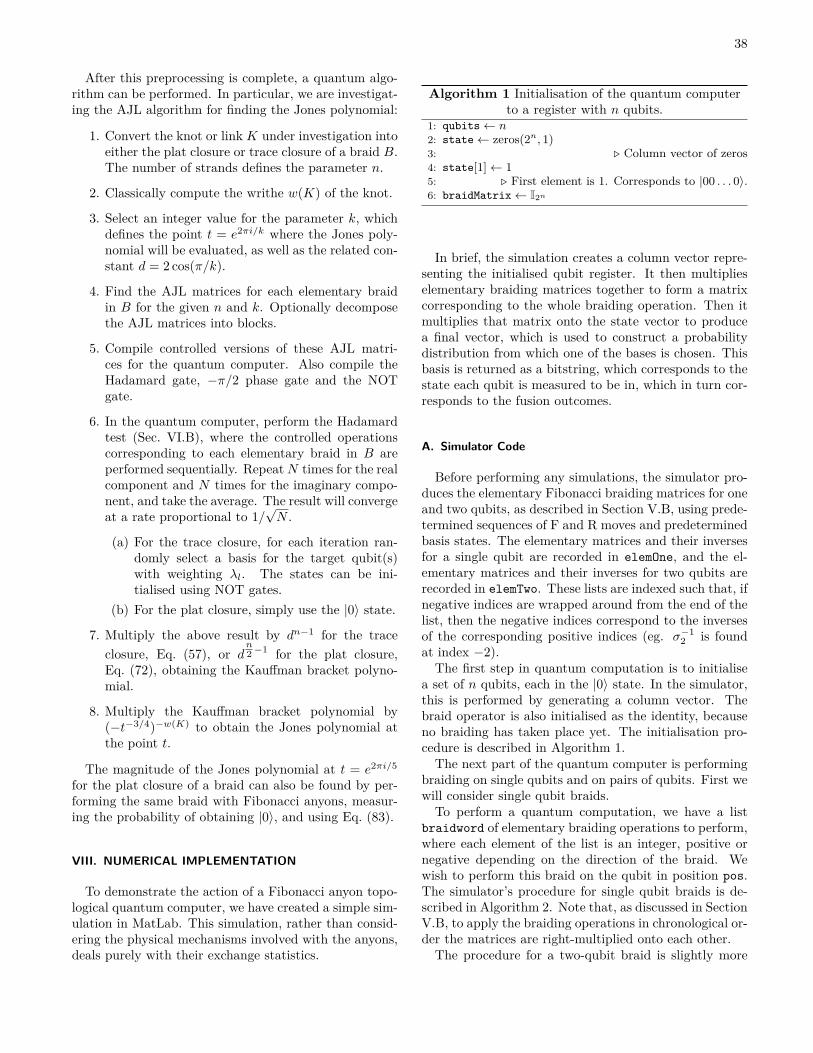
38

After this preprocessing is complete, a quantum algo-rithm can be performed. In particular, we are investigat-ing the AJL algorithm for finding the Jones polynomial:

1. Convert the knot or link K under investigation intoeither the plat closure or trace closure of a braid B.The number of strands defines the parameter n.

2. Classically compute the writhe w(K) of the knot.

3. Select an integer value for the parameter k, whichdefines the point t = e2πi/k where the Jones poly-nomial will be evaluated, as well as the related con-stant d = 2 cos(π/k).

4. Find the AJL matrices for each elementary braidin B for the given n and k. Optionally decomposethe AJL matrices into blocks.

5. Compile controlled versions of these AJL matri-ces for the quantum computer. Also compile theHadamard gate, −π/2 phase gate and the NOTgate.

6. In the quantum computer, perform the Hadamardtest (Sec. VI.B), where the controlled operationscorresponding to each elementary braid in B areperformed sequentially. RepeatN times for the realcomponent and N times for the imaginary compo-nent, and take the average. The result will convergeat a rate proportional to 1/

√N .

(a) For the trace closure, for each iteration ran-domly select a basis for the target qubit(s)with weighting λl. The states can be ini-tialised using NOT gates.

(b) For the plat closure, simply use the |0〉 state.7. Multiply the above result by dn−1 for the trace

closure, Eq. (57), or dn2−1 for the plat closure,

Eq. (72), obtaining the Kauffman bracket polyno-mial.

8. Multiply the Kauffman bracket polynomial by(−t−3/4)−w(K) to obtain the Jones polynomial atthe point t.

The magnitude of the Jones polynomial at t = e2πi/5

for the plat closure of a braid can also be found by per-forming the same braid with Fibonacci anyons, measur-ing the probability of obtaining |0〉, and using Eq. (83).

VIII. NUMERICAL IMPLEMENTATION

To demonstrate the action of a Fibonacci anyon topo-logical quantum computer, we have created a simple sim-ulation in MatLab. This simulation, rather than consid-ering the physical mechanisms involved with the anyons,deals purely with their exchange statistics.

Algorithm 1 Initialisation of the quantum computerto a register with n qubits.

1: qubits← n2: state← zeros(2n, 1)3: . Column vector of zeros4: state[1]← 15: . First element is 1. Corresponds to |00 . . . 0〉.6: braidMatrix← I2n

In brief, the simulation creates a column vector repre-senting the initialised qubit register. It then multiplieselementary braiding matrices together to form a matrixcorresponding to the whole braiding operation. Then itmultiplies that matrix onto the state vector to producea final vector, which is used to construct a probabilitydistribution from which one of the bases is chosen. Thisbasis is returned as a bitstring, which corresponds to thestate each qubit is measured to be in, which in turn cor-responds to the fusion outcomes.

A. Simulator Code

Before performing any simulations, the simulator pro-duces the elementary Fibonacci braiding matrices for oneand two qubits, as described in Section V.B, using prede-termined sequences of F and R moves and predeterminedbasis states. The elementary matrices and their inversesfor a single qubit are recorded in elemOne, and the el-ementary matrices and their inverses for two qubits arerecorded in elemTwo. These lists are indexed such that, ifnegative indices are wrapped around from the end of thelist, then the negative indices correspond to the inversesof the corresponding positive indices (eg. σ−1

2 is foundat index −2).The first step in quantum computation is to initialise

a set of n qubits, each in the |0〉 state. In the simulator,this is performed by generating a column vector. Thebraid operator is also initialised as the identity, becauseno braiding has taken place yet. The initialisation pro-cedure is described in Algorithm 1.The next part of the quantum computer is performing

braiding on single qubits and on pairs of qubits. First wewill consider single qubit braids.To perform a quantum computation, we have a list

braidword of elementary braiding operations to perform,where each element of the list is an integer, positive ornegative depending on the direction of the braid. Wewish to perform this braid on the qubit in position pos.The simulator’s procedure for single qubit braids is de-scribed in Algorithm 2. Note that, as discussed in SectionV.B, to apply the braiding operations in chronological or-der the matrices are right-multiplied onto each other.The procedure for a two-qubit braid is slightly more

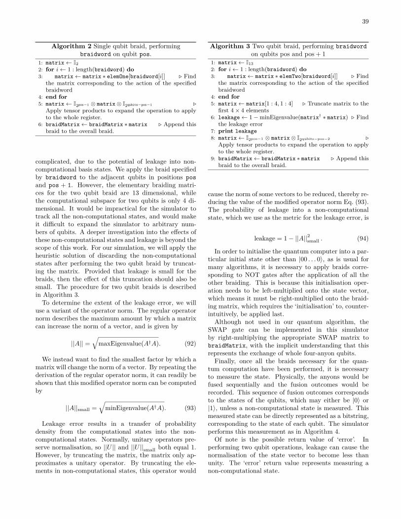
39

Algorithm 2 Single qubit braid, performingbraidword on qubit pos.

1: matrix← I22: for i← 1 : length(braidword) do3: matrix← matrix ∗ elemOne[braidword[i]] . Find

the matrix corresponding to the action of the specifiedbraidword

4: end for5: matrix← I2pos−1 ⊗ matrix⊗ I2qubits−pos−1 .

Apply tensor products to expand the operation to applyto the whole register.

6: braidMatrix← braidMatrix ∗ matrix . Append thisbraid to the overall braid.

complicated, due to the potential of leakage into non-computational basis states. We apply the braid specifiedby braidword to the adjacent qubits in positions posand pos + 1. However, the elementary braiding matri-ces for the two qubit braid are 13 dimensional, whilethe computational subspace for two qubits is only 4 di-mensional. It would be impractical for the simulator totrack all the non-computational states, and would makeit difficult to expand the simulator to arbitrary num-bers of qubits. A deeper investigation into the effects ofthese non-computational states and leakage is beyond thescope of this work. For our simulation, we will apply theheuristic solution of discarding the non-computationalstates after performing the two qubit braid by truncat-ing the matrix. Provided that leakage is small for thebraids, then the effect of this truncation should also besmall. The procedure for two qubit braids is describedin Algorithm 3.

To determine the extent of the leakage error, we willuse a variant of the operator norm. The regular operatornorm describes the maximum amount by which a matrixcan increase the norm of a vector, and is given by

||A|| =√

maxEigenvalue(A†A). (92)

We instead want to find the smallest factor by which amatrix will change the norm of a vector. By repeating thederivation of the regular operator norm, it can readily beshown that this modified operator norm can be computedby

||A||small =√

minEigenvalue(A†A). (93)

Leakage error results in a transfer of probabilitydensity from the computational states into the non-computational states. Normally, unitary operators pre-serve normalisation, so ||U || and ||U ||small both equal 1.However, by truncating the matrix, the matrix only ap-proximates a unitary operator. By truncating the ele-ments in non-computational states, this operator would

Algorithm 3 Two qubit braid, performing braidwordon qubits pos and pos + 1

1: matrix← I132: for i← 1 : length(braidword) do3: matrix← matrix ∗ elemTwo[braidword[i]] . Find

the matrix corresponding to the action of the specifiedbraidword

4: end for5: matrix← matrix[1 : 4, 1 : 4] . Truncate matrix to the

first 4× 4 elements6: leakage← 1−minEigenvalue(matrix† ∗ matrix) . Find

the leakage error7: print leakage8: matrix← I2pos−1 ⊗ matrix⊗ I2qubits−pos−2 .

Apply tensor products to expand the operation to applyto the whole register.

9: braidMatrix← braidMatrix ∗ matrix . Append thisbraid to the overall braid.

cause the norm of some vectors to be reduced, thereby re-ducing the value of the modified operator norm Eq. (93).The probability of leakage into a non-computationalstate, which we use as the metric for the leakage error, is

leakage = 1− ||A||2small . (94)

In order to initialise the quantum computer into a par-ticular initial state other than |00 . . . 0〉, as is usual formany algorithms, it is necessary to apply braids corre-sponding to NOT gates after the application of all theother braiding. This is because this initialisation oper-ation needs to be left-multiplied onto the state vector,which means it must be right-multiplied onto the braid-ing matrix, which requires the ‘initialisation’ to, counter-intuitively, be applied last.Although not used in our quantum algorithm, the

SWAP gate can be implemented in this simulatorby right-multiplying the appropriate SWAP matrix tobraidMatrix, with the implicit understanding that thisrepresents the exchange of whole four-anyon qubits.Finally, once all the braids necessary for the quan-

tum computation have been performed, it is necessaryto measure the state. Physically, the anyons would befused sequentially and the fusion outcomes would berecorded. This sequence of fusion outcomes correspondsto the states of the qubits, which may either be |0〉 or|1〉, unless a non-computational state is measured. Thismeasured state can be directly represented as a bitstring,corresponding to the state of each qubit. The simulatorperforms this measurement as in Algorithm 4.Of note is the possible return value of ‘error’. In

performing two qubit operations, leakage can cause thenormalisation of the state vector to become less thanunity. The ‘error’ return value represents measuring anon-computational state.

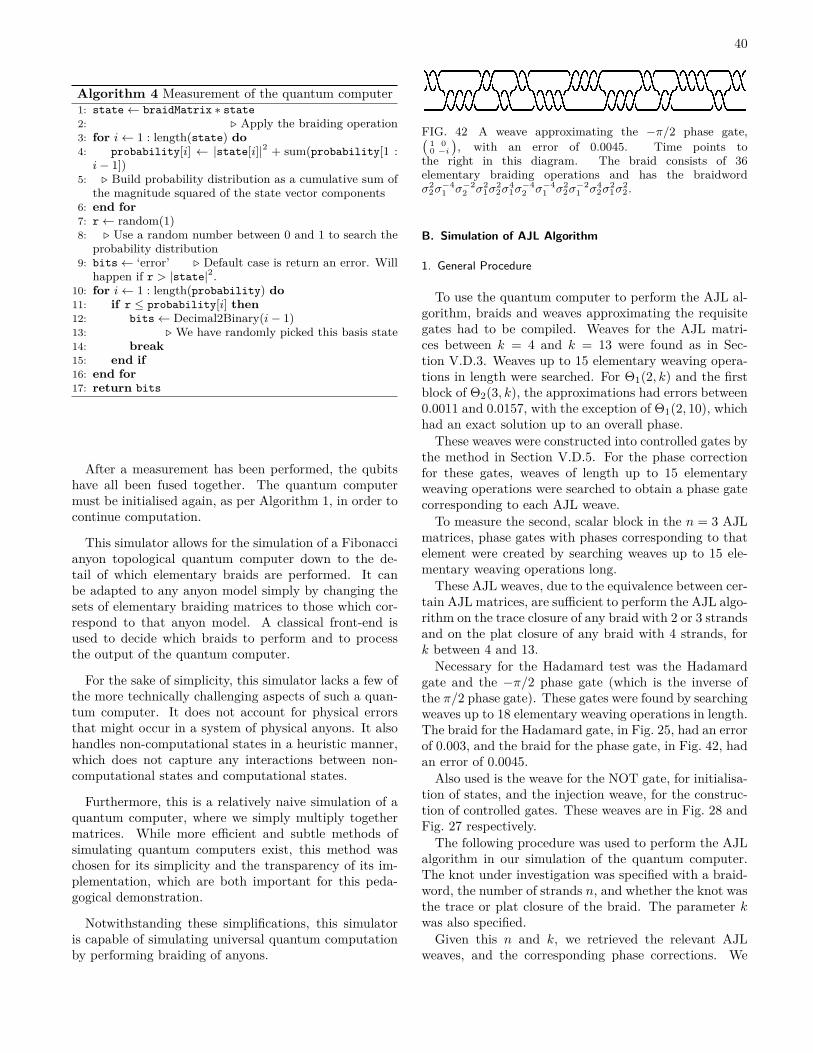
40

Algorithm 4 Measurement of the quantum computer1: state← braidMatrix ∗ state2: . Apply the braiding operation3: for i← 1 : length(state) do4: probability[i] ← |state[i]|2 + sum(probability[1 :i− 1])

5: . Build probability distribution as a cumulative sum ofthe magnitude squared of the state vector components

6: end for7: r← random(1)8: . Use a random number between 0 and 1 to search the

probability distribution9: bits← ‘error’ . Default case is return an error. Will

happen if r > |state|2.10: for i← 1 : length(probability) do11: if r ≤ probability[i] then12: bits← Decimal2Binary(i− 1)13: . We have randomly picked this basis state14: break15: end if16: end for17: return bits

After a measurement has been performed, the qubitshave all been fused together. The quantum computermust be initialised again, as per Algorithm 1, in order tocontinue computation.

This simulator allows for the simulation of a Fibonaccianyon topological quantum computer down to the de-tail of which elementary braids are performed. It canbe adapted to any anyon model simply by changing thesets of elementary braiding matrices to those which cor-respond to that anyon model. A classical front-end isused to decide which braids to perform and to processthe output of the quantum computer.

For the sake of simplicity, this simulator lacks a few ofthe more technically challenging aspects of such a quan-tum computer. It does not account for physical errorsthat might occur in a system of physical anyons. It alsohandles non-computational states in a heuristic manner,which does not capture any interactions between non-computational states and computational states.

Furthermore, this is a relatively naive simulation of aquantum computer, where we simply multiply togethermatrices. While more efficient and subtle methods ofsimulating quantum computers exist, this method waschosen for its simplicity and the transparency of its im-plementation, which are both important for this peda-gogical demonstration.

Notwithstanding these simplifications, this simulatoris capable of simulating universal quantum computationby performing braiding of anyons.

FIG. 42 A weave approximating the −π/2 phase gate,(1 00 −i

), with an error of 0.0045. Time points to

the right in this diagram. The braid consists of 36elementary braiding operations and has the braidwordσ2

2σ−41 σ−2

2 σ21σ

22σ

41σ−42 σ−4

1 σ22σ−21 σ4

2σ21σ

22 .

B. Simulation of AJL Algorithm

1. General Procedure

To use the quantum computer to perform the AJL al-gorithm, braids and weaves approximating the requisitegates had to be compiled. Weaves for the AJL matri-ces between k = 4 and k = 13 were found as in Sec-tion V.D.3. Weaves up to 15 elementary weaving opera-tions in length were searched. For Θ1(2, k) and the firstblock of Θ2(3, k), the approximations had errors between0.0011 and 0.0157, with the exception of Θ1(2, 10), whichhad an exact solution up to an overall phase.These weaves were constructed into controlled gates by

the method in Section V.D.5. For the phase correctionfor these gates, weaves of length up to 15 elementaryweaving operations were searched to obtain a phase gatecorresponding to each AJL weave.To measure the second, scalar block in the n = 3 AJL

matrices, phase gates with phases corresponding to thatelement were created by searching weaves up to 15 ele-mentary weaving operations long.These AJL weaves, due to the equivalence between cer-

tain AJL matrices, are sufficient to perform the AJL algo-rithm on the trace closure of any braid with 2 or 3 strandsand on the plat closure of any braid with 4 strands, fork between 4 and 13.Necessary for the Hadamard test was the Hadamard

gate and the −π/2 phase gate (which is the inverse ofthe π/2 phase gate). These gates were found by searchingweaves up to 18 elementary weaving operations in length.The braid for the Hadamard gate, in Fig. 25, had an errorof 0.003, and the braid for the phase gate, in Fig. 42, hadan error of 0.0045.Also used is the weave for the NOT gate, for initialisa-

tion of states, and the injection weave, for the construc-tion of controlled gates. These weaves are in Fig. 28 andFig. 27 respectively.The following procedure was used to perform the AJL

algorithm in our simulation of the quantum computer.The knot under investigation was specified with a braid-word, the number of strands n, and whether the knot wasthe trace or plat closure of the braid. The parameter kwas also specified.Given this n and k, we retrieved the relevant AJL

weaves, and the corresponding phase corrections. We

41

concatenated the AJL weaves into a single longer weavein the order specified by the knot’s braidword, then usedthe method in Sec. V.D.5 to convert that into a con-trolled operation, with the first qubit being the controlqubit. The corresponding phase corrections were thenapplied to the control qubit. This concatenation wasdone, rather than applying individual controlled oper-ations for each braid in the knot, because adjacent injec-tion weaves would cancel each other out, and thus wouldbe redundant. The phase gates on the first qubit com-mute with the controlled operations, so they were appliedafterwards.

This larger weave was used as the controlled gatewithin the Hadamard test, with the whole controlledgate performed as a single two-qubit weave. The restof the Hadamard test used the weaves corresponding tothe Hadamard gate and −π/2 phase gate. When measur-ing the Markov trace, the state of the second qubit wasdetermined randomly based on a distribution weightedby λl (Eq. (60)). The qubit could be initialised to the|1〉 state by applying the weave approximating the NOTgate. A representative braid corresponding to a compu-tation is given in Fig. 43.

After all weaving had been performed, the state wasmeasured. If the first bit of the returned bitstring was0, then the Hadamard test returned 1. If the first bitwas 1, then the Hadamard test returned −1. This wasperformed for a specified number of iterations for eachof the real and imaginary outputs, and the mean of theoutputs for each component was taken. This numberwas the approximation of the Markov trace for the traceclosure or the first matrix element for the plat closure.

The writhe of the knot was calculated classically, andthen the appropriate factors were multiplied to the resultof the Hadamard test to give an approximation to theJones polynomial at the point t = e2πi/k.

The Hadamard test is stochastic in nature. The resultsin Table I were used to estimate the confidence intervalsfor a given output of the Hadamard test. For the con-fidence interval for that point in the Jones polynomial,the figure for the Hadamard test was multiplied by dn−1

for the trace closure or dn2−1 for the plat closure. In our

results, we reported the 95% confidence interval for eachdata point in the Jones polynomial as error bars.

Because our quantum computer is a classical simula-tion, we were able to access information that would notbe measurable in a real quantum computer. As a mea-sure of comparison to the stochastic results, we directlyread the components of the state vector and the proba-bility of measuring each qubit in a given state, bypassingthe random nature of Algorithm 4. This was used to pre-cisely determine the expectation value of the Hadamardtest for a given set of weaves in the quantum computer.This, in turn, gave the output of the stochastic measure-ments in the limit of an infinite number of iterations.

This quantity is not affected by the stochastic natureof the regular measurements, but it is affected by howclosely the given weaves approximate the intended oper-ations. As such, this metric, although inaccessible to areal quantum computer, provides a measure of the qual-ity of the weaves, and indicates where the measurementwill converge to.Because the knots under investigation were relatively

simple, we verified the output of the quantum AJL algo-rithm against the known analytical solution for the Jonespolynomial.For the braids we have generated, the difference be-

tween the exact value of the Jones polynomial and theresult given by braiding in the limit of infinite iterationswas typically of the order of 0.01. As such, for our mea-surements in the AJL algorithm, we used 10,000 itera-tions of the Hadamard test, which gave a precision ofthe same order of magnitude. More iterations would besuperfluous for our weaves, for it would give greater pre-cision than accuracy.The time complexity of the algorithm as performed

by this simulated quantum computer was quantified bycounting the number of elementary braiding operationsperformed. If it is assumed, in a physical implementa-tion, that each elementary braid takes some fixed amountof time and that the computer spends most of its timebraiding, then the number of elementary braiding oper-ations taken to run an algorithm is directly proportionalto the time a physical quantum computer would spendrunning the algorithm.For the special case of evaluating the magnitude of the

Jones polynomial when k = 5, a simpler procedure wasused. For all the knots tested, they can be expressed asthe plat closure of a braid with four strands, and sincea single qubit contains four anyons the quantum com-puter was initialised to have a single qubit. A singlequbit braid exactly matching the braidword correspond-ing to the physical knot was applied. Measurement wasperformed, and the process was repeated for a desirednumber of iterations. The ratio of the number of times|0〉 was measured to the number of iterations was taken tobe the measured value of Pr(|0〉), which was then appliedto Eq. (83). A representative braid for this computationis in Fig. 44.Because this was a Bernoulli experiment, where the

number of |0〉 outcomes were simply counted, the confi-dence interval for the measured Pr(|0〉) was approximatedusing a method for determining binomial confidence in-tervals, namely the Wilson score interval (Wallis, 2013),which can be calculated as follows. We empirically mea-sure a probability of p over N iterations. We want to findthe (1−α)×100% confidence interval (so 95% would haveα = 0.05). The corresponding quartile is

z = probit(1− α/2) =√

2 erf−1(1− α), (95)

where erf−1 is the inverse error function. Define the re-

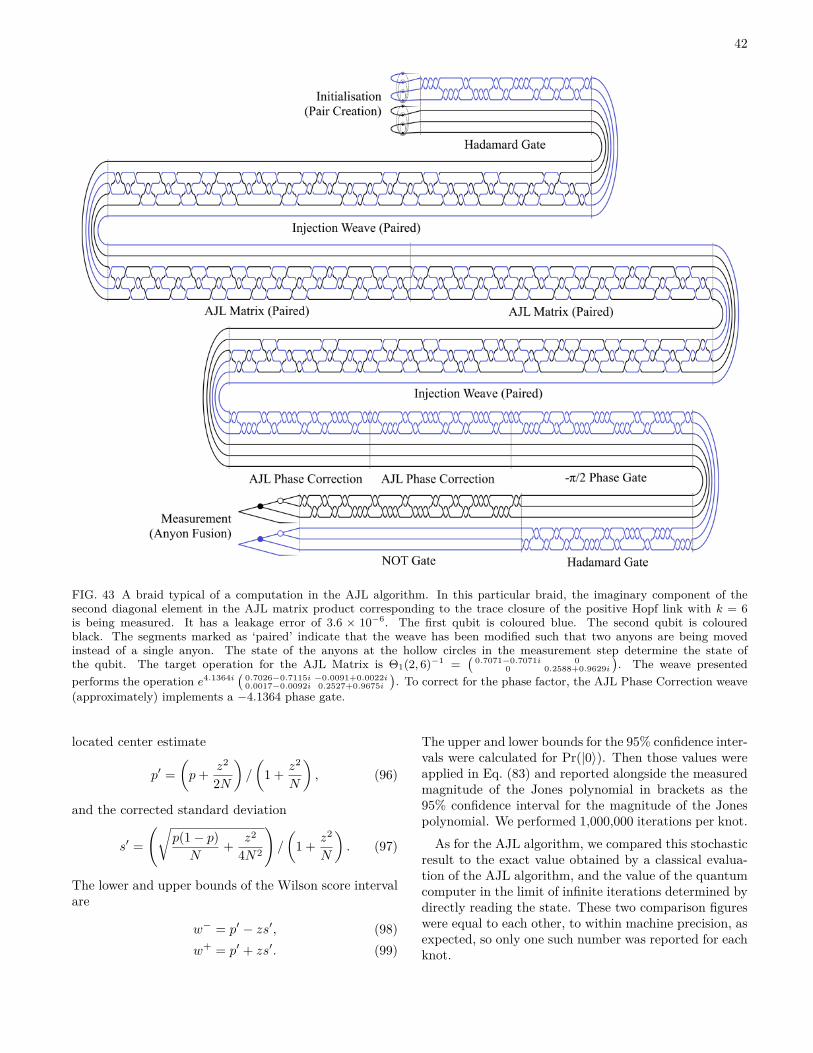
42

FIG. 43 A braid typical of a computation in the AJL algorithm. In this particular braid, the imaginary component of thesecond diagonal element in the AJL matrix product corresponding to the trace closure of the positive Hopf link with k = 6is being measured. It has a leakage error of 3.6 × 10−6. The first qubit is coloured blue. The second qubit is colouredblack. The segments marked as ‘paired’ indicate that the weave has been modified such that two anyons are being movedinstead of a single anyon. The state of the anyons at the hollow circles in the measurement step determine the state ofthe qubit. The target operation for the AJL Matrix is Θ1(2, 6)−1 =

( 0.7071−0.7071i 00 0.2588+0.9629i

). The weave presented

performs the operation e4.1364i( 0.7026−0.7115i −0.0091+0.0022i

0.0017−0.0092i 0.2527+0.9675i

). To correct for the phase factor, the AJL Phase Correction weave

(approximately) implements a −4.1364 phase gate.

located center estimate

p′ =(p+ z2

2N

)/

(1 + z2

N

), (96)

and the corrected standard deviation

s′ =(√

p(1− p)N

+ z2

4N2

)/

(1 + z2

N

). (97)

The lower and upper bounds of the Wilson score intervalare

w− = p′ − zs′, (98)w+ = p′ + zs′. (99)

The upper and lower bounds for the 95% confidence inter-vals were calculated for Pr(|0〉). Then those values wereapplied in Eq. (83) and reported alongside the measuredmagnitude of the Jones polynomial in brackets as the95% confidence interval for the magnitude of the Jonespolynomial. We performed 1,000,000 iterations per knot.As for the AJL algorithm, we compared this stochastic

result to the exact value obtained by a classical evalua-tion of the AJL algorithm, and the value of the quantumcomputer in the limit of infinite iterations determined bydirectly reading the state. These two comparison figureswere equal to each other, to within machine precision, asexpected, so only one such number was reported for eachknot.

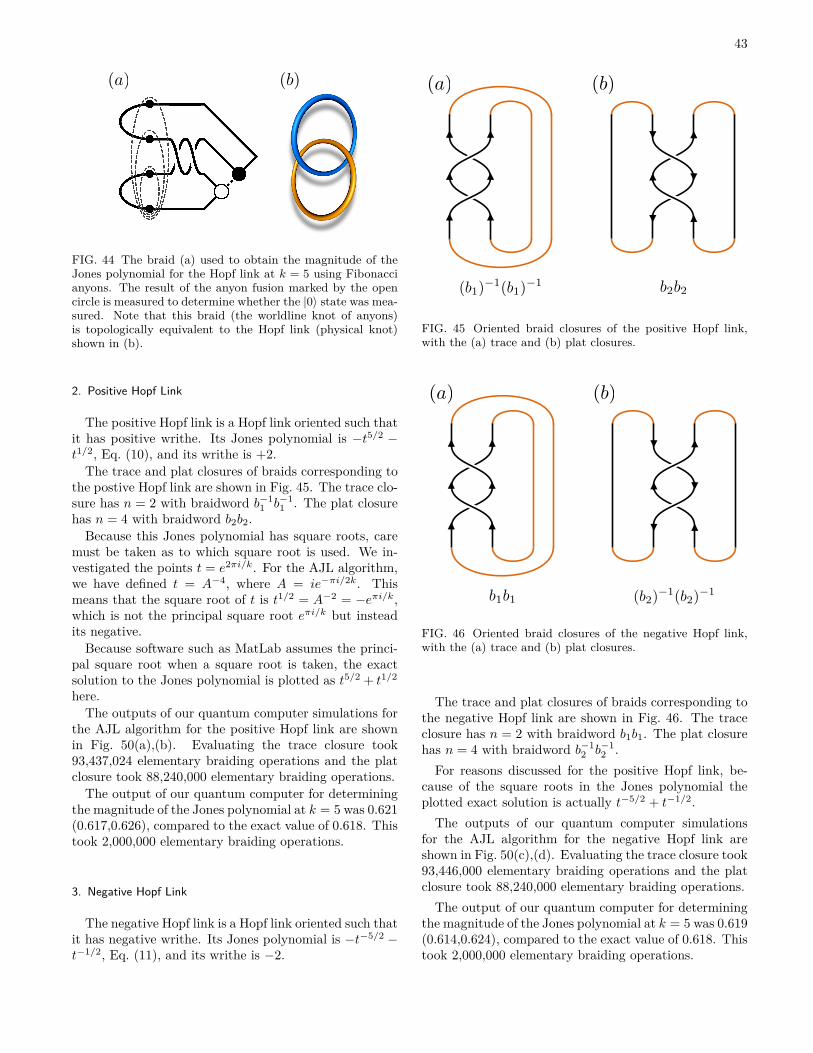
43

(a) (b)

FIG. 44 The braid (a) used to obtain the magnitude of theJones polynomial for the Hopf link at k = 5 using Fibonaccianyons. The result of the anyon fusion marked by the opencircle is measured to determine whether the |0〉 state was mea-sured. Note that this braid (the worldline knot of anyons)is topologically equivalent to the Hopf link (physical knot)shown in (b).

2. Positive Hopf Link

The positive Hopf link is a Hopf link oriented such thatit has positive writhe. Its Jones polynomial is −t5/2 −t1/2, Eq. (10), and its writhe is +2.The trace and plat closures of braids corresponding to

the postive Hopf link are shown in Fig. 45. The trace clo-sure has n = 2 with braidword b−1

1 b−11 . The plat closure

has n = 4 with braidword b2b2.Because this Jones polynomial has square roots, care

must be taken as to which square root is used. We in-vestigated the points t = e2πi/k. For the AJL algorithm,we have defined t = A−4, where A = ie−πi/2k. Thismeans that the square root of t is t1/2 = A−2 = −eπi/k,which is not the principal square root eπi/k but insteadits negative.

Because software such as MatLab assumes the princi-pal square root when a square root is taken, the exactsolution to the Jones polynomial is plotted as t5/2 + t1/2

here.The outputs of our quantum computer simulations for

the AJL algorithm for the positive Hopf link are shownin Fig. 50(a),(b). Evaluating the trace closure took93,437,024 elementary braiding operations and the platclosure took 88,240,000 elementary braiding operations.

The output of our quantum computer for determiningthe magnitude of the Jones polynomial at k = 5 was 0.621(0.617,0.626), compared to the exact value of 0.618. Thistook 2,000,000 elementary braiding operations.

3. Negative Hopf Link

The negative Hopf link is a Hopf link oriented such thatit has negative writhe. Its Jones polynomial is −t−5/2 −t−1/2, Eq. (11), and its writhe is −2.

(a) (b)

(b1)�1(b1)

�1 b2b2

FIG. 45 Oriented braid closures of the positive Hopf link,with the (a) trace and (b) plat closures.

(a) (b)

b1b1 (b2)�1(b2)

�1

FIG. 46 Oriented braid closures of the negative Hopf link,with the (a) trace and (b) plat closures.

The trace and plat closures of braids corresponding tothe negative Hopf link are shown in Fig. 46. The traceclosure has n = 2 with braidword b1b1. The plat closurehas n = 4 with braidword b−1

2 b−12 .

For reasons discussed for the positive Hopf link, be-cause of the square roots in the Jones polynomial theplotted exact solution is actually t−5/2 + t−1/2.The outputs of our quantum computer simulations

for the AJL algorithm for the negative Hopf link areshown in Fig. 50(c),(d). Evaluating the trace closure took93,446,000 elementary braiding operations and the platclosure took 88,240,000 elementary braiding operations.The output of our quantum computer for determining

the magnitude of the Jones polynomial at k = 5 was 0.619(0.614,0.624), compared to the exact value of 0.618. Thistook 2,000,000 elementary braiding operations.

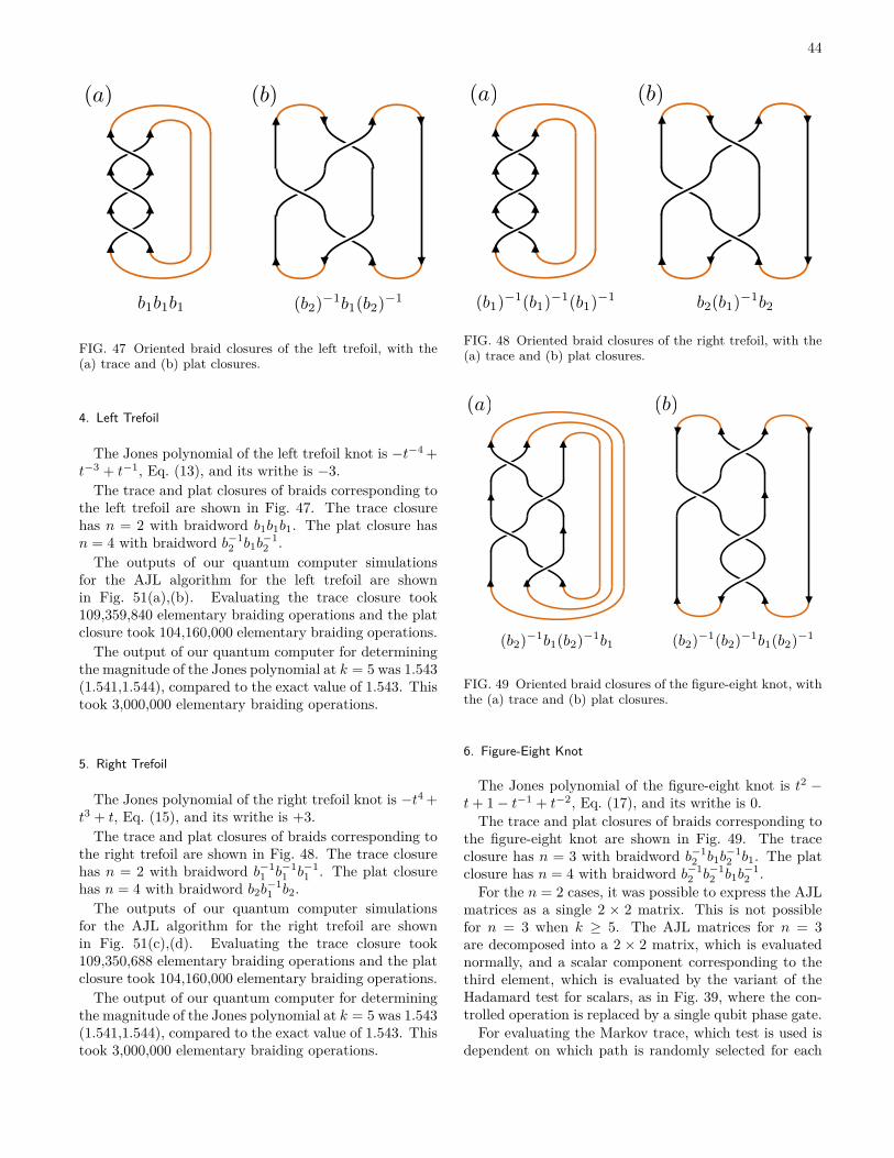
44

(a) (b)

(b2)�1b1(b2)

�1b1b1b1

FIG. 47 Oriented braid closures of the left trefoil, with the(a) trace and (b) plat closures.

4. Left Trefoil

The Jones polynomial of the left trefoil knot is −t−4 +t−3 + t−1, Eq. (13), and its writhe is −3.The trace and plat closures of braids corresponding to

the left trefoil are shown in Fig. 47. The trace closurehas n = 2 with braidword b1b1b1. The plat closure hasn = 4 with braidword b−1

2 b1b−12 .

The outputs of our quantum computer simulationsfor the AJL algorithm for the left trefoil are shownin Fig. 51(a),(b). Evaluating the trace closure took109,359,840 elementary braiding operations and the platclosure took 104,160,000 elementary braiding operations.

The output of our quantum computer for determiningthe magnitude of the Jones polynomial at k = 5 was 1.543(1.541,1.544), compared to the exact value of 1.543. Thistook 3,000,000 elementary braiding operations.

5. Right Trefoil

The Jones polynomial of the right trefoil knot is −t4 +t3 + t, Eq. (15), and its writhe is +3.

The trace and plat closures of braids corresponding tothe right trefoil are shown in Fig. 48. The trace closurehas n = 2 with braidword b−1

1 b−11 b−1

1 . The plat closurehas n = 4 with braidword b2b

−11 b2.

The outputs of our quantum computer simulationsfor the AJL algorithm for the right trefoil are shownin Fig. 51(c),(d). Evaluating the trace closure took109,350,688 elementary braiding operations and the platclosure took 104,160,000 elementary braiding operations.

The output of our quantum computer for determiningthe magnitude of the Jones polynomial at k = 5 was 1.543(1.541,1.544), compared to the exact value of 1.543. Thistook 3,000,000 elementary braiding operations.

(a) (b)

(b1)�1(b1)

�1(b1)�1 b2(b1)

�1b2

FIG. 48 Oriented braid closures of the right trefoil, with the(a) trace and (b) plat closures.

(a) (b)

(b2)�1b1(b2)

�1b1 (b2)�1(b2)

�1b1(b2)�1

FIG. 49 Oriented braid closures of the figure-eight knot, withthe (a) trace and (b) plat closures.

6. Figure-Eight Knot

The Jones polynomial of the figure-eight knot is t2 −t+ 1− t−1 + t−2, Eq. (17), and its writhe is 0.The trace and plat closures of braids corresponding to

the figure-eight knot are shown in Fig. 49. The traceclosure has n = 3 with braidword b−1

2 b1b−12 b1. The plat

closure has n = 4 with braidword b−12 b−1

2 b1b−12 .

For the n = 2 cases, it was possible to express the AJLmatrices as a single 2 × 2 matrix. This is not possiblefor n = 3 when k ≥ 5. The AJL matrices for n = 3are decomposed into a 2 × 2 matrix, which is evaluatednormally, and a scalar component corresponding to thethird element, which is evaluated by the variant of theHadamard test for scalars, as in Fig. 39, where the con-trolled operation is replaced by a single qubit phase gate.For evaluating the Markov trace, which test is used is

dependent on which path is randomly selected for each

45

iteration. Some iterations run the regular 2 × 2 matrixHadamard test, while the other iterations run the scalarHadamard test.

The outputs of our quantum computer simulations forthe AJL algorithm for the figure-eight knot are shownin Fig. 51(e),(f). Evaluating the trace closure took85,217,804 elementary braiding operations and the platclosure took 120,480,000 elementary braiding operations.

The output of our quantum computer for determiningthe magnitude of the Jones polynomial at k = 5 was 1.235(1.232,1.238), compared to the exact value of 1.236. Thistook 4,000,000 elementary braiding operations.

C. Discussion

Convergence of the AJL algorithm to the Jones poly-nomial is determined by multiple factors. The precisionis determined primarily by the number of iterations ofthe Hadamard test, with more iterations and repeatedmeasurements resulting in a convergence at a rate pro-portional to 1/

√N .

The precision is also influenced by the size of the knot.The output of the quantum computer is scaled by dn−1

or dn2−1 for trace or plat closures respectively, where

2 > d > 1 for k > 3. The breadth of the confidenceinterval, or the uncertainty produced by the stochasticnature of the measurement, is also scaled by that fac-tor, meaning knots with more strands and thus highern would have larger uncertainties in the measurement ofthe Jones polynomial, all else being equal. This is whythe error bars for the trace closure of the figure-eight knotwhich has n = 3, shown in Fig. 51(e), are approximately0.2 wide while other knots with n = 2 have error barsunder 0.1 in width.

The accuracy of the results of the AJL algorithm, orany algorithm, performed with a topological quantumcomputer is dependent on the accuracy of the braids usedto approximate the various unitary operators. Even withan infinite number of iterations of the AJL algorithm,where the uncertainty due to stochastic variations hasbeen reduced to zero, the results will only be as accurateas the braids used to approximate the unitary operators.To achieve more accurate results, it is necessary to com-pile more accurate braids for all the operators used in thequantum algorithm. These braids have a length propor-tional to log(1/ε), where ε is the error of the approxima-tion.

Suppose you wish to use the quantum AJL algorithmto determine the Jones polynomial for a knot at a pointto within ε of the exact value. The length of the braidsscales as log(1/ε), while the number of iterations forthe Hadamard test scales as 1/ε2. As such, the num-ber of elementary operations needed to perform the AJLalgorithm, and thus the time complexity, will scale asO((1/ε)2 log(1/ε)).

The logarithmic factor is intrinsic to the topologicalquantum computer and independent of the algorithmused. The quadratic factor is specific to the AJL al-gorithm, and reflects the discrete stochastic nature ofmeasurement in the quantum computer. This quadraticfactor would be expected to appear in other quantumalgorithms in which the measured quantity is the proba-bility amplitudes of the states, because the standard de-viation of the binomial distribution scales as

√N so the

standard deviation of a ratio derived from discrete trialswould scale as 1/

√N . However, for other quantum algo-

rithms where the measured quantity is a particular statewhich is observed with high probability, as for Shor’s fac-torisation algorithm (Shor, 1994), then a smaller (possi-bly constant) factor would replace the quadratic factor.Consider the plat closure of the positive Hopf link, as

in Fig. 50(b), where the points are within approximately0.05 of the exact values. It took 88,240,000 elemen-tary braiding operations (with 200,000 measurementsand 800,000 anyon pairs created) to achieve this accuracy.Suppose the experiment is repeated with a target accu-racy of 10−3 for each point. This would require approx-imately 500,000,000 measurements, 2,000,000,000 anyonpairs created and 509,000,000,000 elementary braidingoperations. This is comparable to the amount of braid-ing necessary to use Fibonacci anyons to evaluate Shor’sfactorisation algorithm for a 128-bit number, and wouldlikely take several hours if implemented using electronsin the quantum Hall effect (Baraban et al., 2010).To achieve a precision of around 10−16, which is com-

parable to a classical computer working with 64 bit float-ing point numbers, would require approximately 5×1034

measurements and 3 × 1038 elementary braiding opera-tions, which would be unrealistic in any practical system.This quadratic scaling of the quantum AJL algorithmmeans that, while still efficient in the technical sense, itis impractical if very high precisions are desired.The number of elementary braiding operations needed

to compute the AJL algorithm increases linearly with thelength of the braidword, and thus the number of cross-ings, representing the knot under investigation, sinceeach term in the braidword adds an extra operator tothe computation, which adds a constant number of ele-mentary braiding operations. This linear complexity is asignificant improvement over the exponential complexityof the more direct algorithm presented in Section III.B,albeit at the cost of only being able to evaluate the Jonespolynomial at a discrete number of points.An exception to this trend is observable in the data for

the Jones polynomial calculated from the trace closure.The Hopf link, with a braidword length of 2, took 93million elementary braiding operations to evaluate. Thetrefoil, with a braidword length of 3, took 109 millionelementary braiding operations to evaluate. The figure-eight knot, with a braidword length of 4, took only 85million elementary braiding operations to evaluate. The

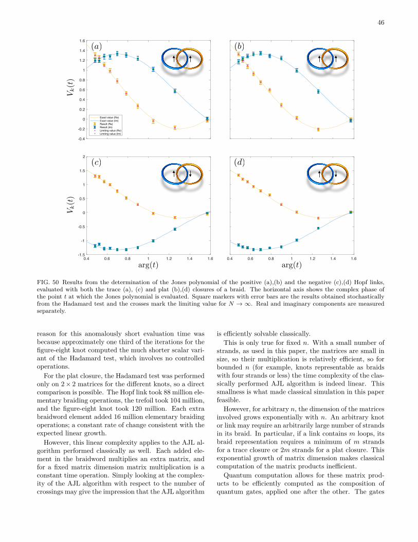
46

0.4 0.6 0.8 1 1.2 1.4 1.6-0.4

-0.2

0

0.2

0.4

0.6

0.8

1

1.2

1.4

1.6

0.4 0.6 0.8 1 1.2 1.4 1.6-1.5

-1

-0.5

0

0.5

1

1.5

2

0.4 0.6 0.8 1 1.2 1.4 1.6-0.4

-0.2

0

0.2

0.4

0.6

0.8

1

1.2

1.4

1.6

Exact value (Re)Exact value (Im)Result (Re)Result (Im)Limiting value (Re)Limiting value (Im)

0.4 0.6 0.8 1 1.2 1.4 1.6-1.5

-1

-0.5

0

0.5

1

1.5

2

(a) (b)

(c) (d)

Vk(t

)V

k(t

)

arg(t) arg(t)

FIG. 50 Results from the determination of the Jones polynomial of the positive (a),(b) and the negative (c),(d) Hopf links,evaluated with both the trace (a), (c) and plat (b),(d) closures of a braid. The horizontal axis shows the complex phase ofthe point t at which the Jones polynomial is evaluated. Square markers with error bars are the results obtained stochasticallyfrom the Hadamard test and the crosses mark the limiting value for N → ∞. Real and imaginary components are measuredseparately.

reason for this anomalously short evaluation time wasbecause approximately one third of the iterations for thefigure-eight knot computed the much shorter scalar vari-ant of the Hadamard test, which involves no controlledoperations.

For the plat closure, the Hadamard test was performedonly on 2× 2 matrices for the different knots, so a directcomparison is possible. The Hopf link took 88 million ele-mentary braiding operations, the trefoil took 104 million,and the figure-eight knot took 120 million. Each extrabraidword element added 16 million elementary braidingoperations; a constant rate of change consistent with theexpected linear growth.

However, this linear complexity applies to the AJL al-gorithm performed classically as well. Each added ele-ment in the braidword multiplies an extra matrix, andfor a fixed matrix dimension matrix multiplication is aconstant time operation. Simply looking at the complex-ity of the AJL algorithm with respect to the number ofcrossings may give the impression that the AJL algorithm

is efficiently solvable classically.This is only true for fixed n. With a small number of

strands, as used in this paper, the matrices are small insize, so their multiplication is relatively efficient, so forbounded n (for example, knots representable as braidswith four strands or less) the time complexity of the clas-sically performed AJL algorithm is indeed linear. Thissmallness is what made classical simulation in this paperfeasible.However, for arbitrary n, the dimension of the matrices

involved grows exponentially with n. An arbitrary knotor link may require an arbitrarily large number of strandsin its braid. In particular, if a link contains m loops, itsbraid representation requires a minimum of m strandsfor a trace closure or 2m strands for a plat closure. Thisexponential growth of matrix dimension makes classicalcomputation of the matrix products inefficient.

Quantum computation allows for these matrix prod-ucts to be efficiently computed as the composition ofquantum gates, applied one after the other. The gates

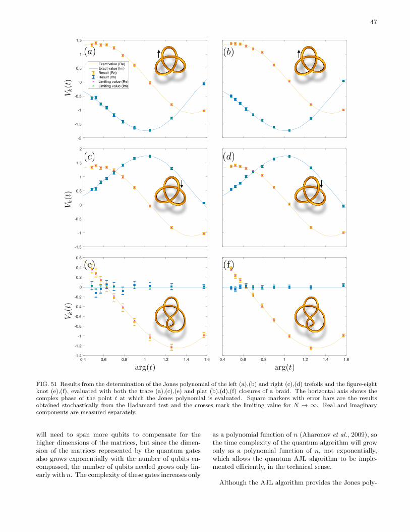
47

0.4 0.6 0.8 1 1.2 1.4 1.6-2

-1.5

-1

-0.5

0

0.5

1

1.5

0.4 0.6 0.8 1 1.2 1.4 1.6-2

-1.5

-1

-0.5

0

0.5

1

1.5

Exact value (Re)Exact value (Im)Result (Re)Result (Im)Limiting value (Re)Limiting value (Im)

0.4 0.6 0.8 1 1.2 1.4 1.6-1.5

-1

-0.5

0

0.5

1

1.5

2

0.4 0.6 0.8 1 1.2 1.4 1.6-1.5

-1

-0.5

0

0.5

1

1.5

2

0.4 0.6 0.8 1 1.2 1.4 1.6-1.4

-1.2

-1

-0.8

-0.6

-0.4

-0.2

0

0.2

0.4

0.6

0.4 0.6 0.8 1 1.2 1.4 1.6-1.4

-1.2

-1

-0.8

-0.6

-0.4

-0.2

0

0.2

0.4

0.6

Vk(t

)V

k(t

)V

k(t

)

(a) (b)

(c) (d)

(e) (f)

arg(t) arg(t)

FIG. 51 Results from the determination of the Jones polynomial of the left (a),(b) and right (c),(d) trefoils and the figure-eightknot (e),(f), evaluated with both the trace (a),(c),(e) and plat (b),(d),(f) closures of a braid. The horizontal axis shows thecomplex phase of the point t at which the Jones polynomial is evaluated. Square markers with error bars are the resultsobtained stochastically from the Hadamard test and the crosses mark the limiting value for N → ∞. Real and imaginarycomponents are measured separately.

will need to span more qubits to compensate for thehigher dimensions of the matrices, but since the dimen-sion of the matrices represented by the quantum gatesalso grows exponentially with the number of qubits en-compassed, the number of qubits needed grows only lin-early with n. The complexity of these gates increases only

as a polynomial function of n (Aharonov et al., 2009), sothe time complexity of the quantum algorithm will growonly as a polynomial function of n, not exponentially,which allows the quantum AJL algorithm to be imple-mented efficiently, in the technical sense.

Although the AJL algorithm provides the Jones poly-

48

nomial at only a discrete set of points, it may in principlebe possible to use it to determine the full Jones poly-nomial using curve fitting. It is possible to determinethe upper and lower bounds on the powers in the Jonespolynomial of a knot without computing the Jones poly-nomial itself (Thistlethwaite, 1988), from which a modelpolynomial for curve fitting can be constructed. The ad-ditional constraints that the Jones polynomial must haveinteger coefficients and is equal to exactly 1 at e2πi/3

would also assist in curve fitting. The disadvantage ofthis approach is that for any large knots the Jones poly-nomial would be a very high order polynomial, whichcould make curve fitting impractical.

Even without the whole polynomial, useful informa-tion can still be extracted from the points provided bythe AJL algorithm. It can be used to distinguish knots,for if two knots have different values of the Jones poly-nomial at any point, then they must have different Jonespolynomials, and thus be inequivalent knots. It can beused to determine whether a knot is chiral or achiral, be-cause the Jones polynomial of achiral knots such as thefigure-eight knot at the roots of unity will have no imag-inary component. And if only the value of the Jonespolynomial at a single point is needed, as in topologicalquantum field theories, then the AJL algorithm is suffi-cient.

The magnitude of the Jones polynomial at t = e2πi/5,as evaluated with Fibonacci anyons without approxima-tions, contains less information than the points obtainedfrom the AJL algorithm, but is much faster to com-pute. Because no braids approximating quantum gatesare used, since all braiding performs the desired opera-tion exactly, the time complexity of the algorithm withrespect to the desired precision scales only as O((1/ε)2),and each iteration requires only exactly as many ele-mentary braiding operations as there are in the knot’sbraidword. This allows for higher precision in the sameamount of time compared to the quantum AJL algo-rithm. Although there is less information provided bythis single point, it can still be used to help distinguishinequivalent knots.

For indicating the error bars for the outputs of the AJLalgorithm, we used the empirically obtained average datafrom Table I. While this is adequate for demonstratingapproximate average behaviour of the percentiles, it doesnot capture the variability between trials in Fig. 41. Amore accurate, albeit more complicated, method of es-timating the uncertainty in the outputs of the AJL al-gorithm would be to analytically derive them using bi-nomial confidence intervals such as the Wilson score in-terval. This would produce a separate asymmetric con-fidence interval for the real and imaginary outputs ofthe Hadamard test. However, determining the behaviourof this elliptical confidence region under rotation in thecomplex plane, as from multiplication by (−t−3/4)−w(K),would have added an unnecessary layer of complexity to

this pedagogical demonstration. The use of the empiri-cally determined average behaviour was adequate for ourpurposes.

IX. CONCLUSIONS

Topological quantum computation is a rich field ofstudy due to its potential fault tolerance imparted by thetopological nature of the underlying systems. Fibonaccianyons are a model of particular interest due to theircapacity to perform universal quantum computation bybraiding alone. Here we have discussed the operationsbraiding performs, how a quantum computer can be de-fined for Fibonacci anyons, and how to construct arbi-trary unitary operations from the braiding of Fibonaccianyons. We have also provided an explanation of the AJLalgorithm for determining the Jones polynomial, and howit may be applied as a quantum algorithm.By performing simulations in MatLab, we have explic-

itly demonstrated the braiding operations required toperform quantum computation with Fibonacci anyons.We have shown how topological quantum computers canbe used to compute the Jones polynomial at roots ofunity and discussed how to generalise these principles togeneric quantum algorithms.We have also demonstrated a connection between Fi-

bonacci anyons and the Jones polynomial at t = e2πi/5,and similarly for Ising anyons and the Jones polyno-mial at t = i, and have conjectured that other anyonmodels with similar relations exist. Since such spe-cific problems can be solved exactly for many knots andlinks using only four non-Abelian anyons correspondingto a single topological qubit, they serve as ideal proofof concept experiments of topological quantum comput-ers. Specifically, using Fibonacci anyons the magnitude|VHopf(ei2π/5)| = (1 +

√5)√

Pr(|0〉5)/2 = (√

5 − 1)/2 ofthe Jones polynomial of the Hopf link at the fifth root ofunity can be obtained using only two elementary physicalbraiding operations and thereafter measuring the annihi-lation probability of the anyons upon fusing them, seeFigs 44 and 13. Similarly for Ising anyons measuringthe magnitude |VHopf(ei2π/4)| =

√2√

Pr(|0〉4) = 0 cor-responds to the non-trivial outcome that after only twoelementary braids that return the anyons to their originalpositions there is a vanishing probability for the anyonsto fuse back to vacuum, where as if no braiding is donethis probability is one. Extending these results to arbi-trary knots or links is straightforward. Similar relationsare anticipated to hold for a broad variety of anyon mod-els.With this practical introduction into the usage of topo-

logical quantum computers, we are looking forward tofurther work performed in this field. An explicit quantumcircuit for performing the AJL algorithm for knots witharbitrary numbers of strands could be designed. The use

49

of anyon braiding to compute the magnitude of the Jonespolynomial at specific roots of unity could be exploredfurther. Other quantum algorithms, such as Shor’s al-gorithm, could be performed using topological quan-tum computation. Braiding statistics for anyon mod-els besides the Fibonacci and Ising anyon models couldbe calculated to allow topological quantum computationwith such models as well. Quantum algorithms couldbe performed in simulators capturing the full physicsof topological quantum computers, and integrated withquantum error correcting codes. And physical experi-ments will continue to search for non-Abelian anyonssuitable for topological quantum computation, so thatonce found, computation can be performed with suchanyons and the results compared with theoretical models.

ACKNOWLEDGMENTS

We acknowledge support from the Australian ResearchCouncil (ARC) via Discovery Project No. DP170104180.

REFERENCES

Abo-Shaeer, J. R., C. Raman, J. M. Vogels, and W. Ketterle(2001), Science 292, 476.

Abrikosov, A. A. (2004), Rev. Mod. Phys. 76, 975.Aharonov, D., V. Jones, and Z. Landau (2009), Algorithmica

55, 395.Aikawa, K., A. Frisch, M. Mark, S. Baier, A. Rietzler,

R. Grimm, and F. Ferlaino (2012), Phys. Rev. Lett. 108,210401.

Ainsworth, R., and J. K. Slingerland (2011), New Journal ofPhysics 13 (6), 065030.

Alexander, J. W. (1923), Proceedings of the NationalAcademy of Sciences 9 (3), 93.

Alicea, J. (2012), Reports on Progress in Physics 75 (7),076501.

Alicea, J., and A. Stern (2015), Physica Scripta Volume T164 (1), 014006.

Ardonne, E., and K. Schoutens (2007), Annals of Physics322 (1), 201.

Autti, S., V. V. Dmitriev, J. T. Mäkinen, A. A. Soldatov,G. E. Volovik, A. N. Yudin, V. V. Zavjalov, and V. B.Eltsov (2016), Physical Review Letters 117 (25), 255301.

Ayeni, B. M., S. Singh, R. N. C. Pfeifer, and G. K. Brennen(2016), Phys. Rev. B 93, 165128.

Baraban, M., N. E. Bonesteel, and S. H. Simon (2010), Phys.Rev. A 81, 062317.

Barenghi, C. F., L. Skrbek, and K. R. Sreenivasan (2014),Proceedings of the National Academy of Science 111, 4647.

Bombin, H., and M. A. Martin-Delgado (2008), Phys. Rev.B 78, 115421.

Bombin, H., and M. A. Martin-Delgado (2011), New Journalof Physics 13 (12), 125001.

Bonderson, P., M. Freedman, and C. Nayak (2008), Phys.Rev. Lett. 101, 010501.

Bonderson, P., K. Shtengel, and J. K. Slingerland (2006),Phys. Rev. Lett. 97, 016401.

Bonesteel, N. E., L. Hormozi, G. Zikos, and S. H. Simon(2005), Phys. Rev. Lett. 95, 140503.

Bonesteel, N. E., L. Hormozi, G. Zikos, and S. H. Simon(2007), International Journal of Modern Physics B 21,1372.

Bordewich, M., M. Freedman, L. Lovász, and D. Welsh(2005), Combinatorics, Probability and Computing 14,737.

Borgh, M. O., and J. Ruostekoski (2016), Phys. Rev. Lett.117, 275302.

Bravyi, S. (2006), Phys. Rev. A 73, 042313.Brennen, G. K., and J. K. Pachos (2008), Proceedings of the

Royal Society A-Mathematical Physical and EngineeringSciences 464, 1.

Burrello, M., G. Mussardo, and X. Wan (2011), New Journalof Physics 13 (2), 025023.

Burrello, M., H. Xu, G. Mussardo, and X. Wan (2010), Phys-ical Review Letters 104 (16), 160502.

Burton, S. (2016), ArXiv e-prints arXiv:1610.05384 [quant-ph].

Burton, S., C. G. Brell, and S. T. Flammia (2017), Phys.Rev. A 95, 022309.

Carnahan, C., D. Zeuch, and N. E. Bonesteel (2016), Phys.Rev. A 93, 052328.

Castelvecchi, D. (2018), Nature (London) 553, 136.Ðurić, T., K. Biedroń, and J. Zakrzewski (2017), Phys. Rev.

B 95, 085102.Cirac, J. I., and P. Zoller (1995), Physical Review Letters

74, 4091.Collins, G. P. (2006a), Scientific American 294 (4), 56.Collins, G. P. (2006b), Sci Am 294, 56.Cooper, N. R., N. K. Wilkin, and J. M. F. Gunn (2001),

Phys. Rev. Lett. 87, 120405.Datta, A., and A. Shaji (2011), International Journal of

Quantum Information 09 (07n08), 1787.Datta, A., A. Shaji, and C. M. Caves (2008), Phys. Rev.

Lett. 100, 050502.Dawson, C. M., and M. A. Nielsen (2006), Quantum Info.

Comput. 6, 81.Dennis, M. R., R. P. King, B. Jack, K. O’Holleran, and M. J.

Padgett (2010), Nature Physics 6, 118.Dicarlo, L., J. M. Chow, J. M. Gambetta, L. S. Bishop, B. R.

Johnson, D. I. Schuster, J. Majer, A. Blais, L. Frunzio,S. M. Girvin, and R. J. Schoelkopf (2009), Nature (Lon-don) 460, 240.

DiVincenzo, D., I. für Festkörperforschung, I. für Festkör-perforschung (Jülich). Spring School, and J. C. for Neu-tron Science (2013), Quantum Information Processing:Lecture Notes of the 44th IFF Spring School 2013 , Schriftendes Forschungszentrums Jülich. Reihe Schlüsseltechnolo-gien / Key Technologies (Forschungszentrum Jülich).

DiVincenzo, D. P. (2000), Fortschritte der Physik 48 (9), 771.Essmann, U., and H. Träuble (1967), Physics Letters A 24,

526.Fendley, P., S. V. Isakov, and M. Troyer (2013), Phys. Rev.

Lett. 110, 260408.Feng, W. (2015), Non-Abelian quantum error correction,

Ph.D. thesis (Florida State University).Fetter, A. L. (2009), Reviews of Modern Physics 81, 647.Feynman, R. P. (1982), International Journal of Theoretical

Physics 21, 467.Fonda, E., D. P. Meichle, N. T. Ouellette, S. Hormoz, and

D. P. Lathrop (2014), Proceedings of the National Academyof Science 111, 4707.

50

Freedman, M. H. (1998), Proceedings of the NationalAcademy of Sciences 95, 98.

Freedman, M. H., A. Kitaev, M. J. Larsen, and Z. Wang(2003), Bulletin of the American Mathematical Society 40,31.

Freedman, M. H., A. Kitaev, and Z. Wang (2002a), Commu-nications in Mathematical Physics 227, 587.

Freedman, M. H., M. Larsen, and Z. Wang (2002b), Com-munications in Mathematical Physics 227, 605.

Freedman, M. H., and Z. Wang (2007), Phys. Rev. A 75,032322.

Galindo, A., and M. A. Martín-Delgado (2002), Rev. Mod.Phys. 74, 347.

Gibney, E. (2016), Nature 10.1038/nature.2016.20774.Griesmaier, A., J. Werner, S. Hensler, J. Stuhler, and T. Pfau

(2005), Phys. Rev. Lett. 94, 160401.Gurarie, V., and L. Radzihovsky (2007), Annals of Physics

322, 2.Hadzibabic, Z., P. Krüger, M. Cheneau, B. Battelier, and

J. Dalibard (2006), Nature (London) 441, 1118.Hakonen, P. J., O. T. Ikkala, and S. T. Islander (1982),

Physical Review Letters 49, 1258.Harrow, A. W., B. Recht, and I. L. Chuang (2002), Journal

of Mathematical Physics 43, 4445.Hormozi, L., N. E. Bonesteel, and S. H. Simon (2009), Phys.

Rev. Lett. 103, 160501.Hormozi, L., G. Zikos, N. E. Bonesteel, and S. H. Simon

(2007), Phys. Rev. B 75, 165310.Huhtamäki, J. A. M., T. P. Simula, M. Kobayashi, and

K. Machida (2009), Phys. Rev. A 80 (5), 051601.Jones, V. F. R. (1985), Bull. Amer. Math. Soc. (N.S.) 12 (1),

103.Kane, B. E. (1998), Nature (London) 393, 133.Kauffman, L., and S. Lomonaco (2007), Mathematics of

Quantum Computation and Quantum Technology, Chap-man & Hall/CRC Applied Mathematics & Nonlinear Sci-ence (CRC Press).

Kauffman, L. H. (2016), “Knot logic and topological quantumcomputing with Majorana fermions,” in Logic and AlgebraicStructures in Quantum Computing, Lecture Notes in Logic,edited by J. Chubb, A. Eskandarian, and V. Harizanov(Cambridge University Press) p. 223.

Kawaguchi, Y., and M. Ueda (2012), Phys. Rep. 520, 253.Kitaev, A. (2003), Annals of Physics 303, 2.Kitaev, A. Y. (1997), Russian Mathematical Surveys 52,

1191.Kleckner, D., and W. T. M. Irvine (2013), Nature Physics 9,

253.Kliuchnikov, V., A. Bocharov, and K. M. Svore (2014), Phys.

Rev. Lett. 112, 140504.Knill, E., R. Laflamme, and G. J. Milburn (2001), Nature

(London) 409, 46.Kobayashi, M., Y. Kawaguchi, M. Nitta, and M. Ueda (2009),

Physical Review Letters 103 (11), 115301.Kobayashi, M., and M. Ueda (2016), .Kosterlitz, J. M. (2017), Rev. Mod. Phys. 89, 040501.Leibfried, D., R. Blatt, C. Monroe, and D. Wineland (2003),

Reviews of Modern Physics 75, 281.Lian, B., T.-L. Ho, and H. Zhai (2012), Phys. Rev. A 85,

051606.Lloyd, S. (1996), Science 273, 1073.Lomonaco, S. J., and L. H. Kauffman (2006), Proc.SPIE

6244, 6244 .Loss, D., and D. P. DiVincenzo (1998), Phys. Rev. A 57,

120.Lu, C.-Y., D. E. Browne, T. Yang, and J.-W. Pan (2007),

Phys. Rev. Lett. 99, 250504.Lu, M., N. Q. Burdick, S. H. Youn, and B. L. Lev (2011),

Phys. Rev. Lett. 107, 190401.Madison, K. W., F. Chevy, W. Wohlleben, and J. Dalibard

(2000), Physical Review Letters 84, 806.Matthews, M. R., B. P. Anderson, P. C. Haljan, D. S. Hall,

C. E. Wieman, and E. A. Cornell (1999), Physical ReviewLetters 83, 2498.

Mawson, T., T. C. Petersen, and T. Simula (2017), Phys.Rev. A 96 (3), 033623.

Mawson, T., T. C. Petersen, and T. Simula (2018), in prepa-ration.

McDonald, R. B., and H. G. Katzgraber (2013), Phys. Rev.B 87, 054414.

Mermin, N. D. (1979), Reviews of Modern Physics 51, 591.Milburn, G. (1996), Quantum Technology, Frontiers of science

(Allen & Unwin).Mizushima, T., M. Ichioka, and K. Machida (2008), Physical

Review Letters 101 (15), 150409.Mochon, C. (2003), Phys. Rev. A 67, 022315.Modi, K., A. Brodutch, H. Cable, T. Paterek, and V. Vedral

(2012), Reviews of Modern Physics 84, 1655.Mong, R. S. K., M. P. Zaletel, F. Pollmann, and Z. Papić

(2017), Phys. Rev. B 95, 115136.Mosseri, R. (2008), Journal of Physics A: Mathematical and

Theoretical 41 (17), 175302.Nakahara, M. (2012), “Computing with quanta,” in Quantum

Information and Quantum Computing (World Scientific)pp. 1–42.

Nayak, C., S. H. Simon, A. Stern, M. Freedman, and S. D.Sarma (2008), Reviews of Modern Physics 80, 1083.

Nielsen, M., and I. Chuang (2010), Quantum Computa-tion and Quantum Information : 10th Anniversary Edition(Cambridge University Press).

Nikolova, A., G. K. Brennen, T. J. Osborne, G. J. Milburn,and T. M. Stace (2018), Phys. Rev. A 97, 030101.

Pachos, J. K. (2012), Introduction to Topological QuantumComputation (Cambridge University Press).

Pachos, J. K., and S. H. Simon (2014), New Journal ofPhysics 16 (6), 065003.

Pednault, E., J. A. Gunnels, G. Nannicini, L. Horesh,T. Magerlein, E. Solomonik, and R. Wisnieff (2017), ArXive-prints arXiv:1710.05867 [quant-ph].

Petersen, T. C., M. Weyland, D. M. Paganin, T. P. Simula,S. A. Eastwood, and M. J. Morgan (2013), Physical ReviewLetters 110 (3), 033901.

Preskill, J. (1997), arXiv:quant-ph/9712048.Preskill, J. (2004), “Lecture notes for physics

219: Quantum computation,” Available atwww.theory.caltech.edu/∼preskill/ph219/topological.pdf.

Raedt, K. D., K. Michielsen, H. D. Raedt, B. Trieu,G. Arnold, M. Richter, T. Lippert, H. Watanabe, andN. Ito (2007), Computer Physics Communications 176 (2),121 .

Reilly, D. J., J. M. Taylor, J. R. Petta, C. M. Marcus, M. P.Hanson, and A. C. Gossard (2008), Science 321, 817.

Rezayi, E. H., and N. Read (2009), Phys. Rev. B 79, 075306.Roberts, K. O., T. McKellar, J. Fekete, A. Rakonjac, A. B.

Deb, and N. Kjærgaard (2014), Optics Letters 39, 2012.Ross, N. J., and P. Selinger (2014), ArXiv e-prints

arXiv:1403.2975 [quant-ph].Samson, E. C., K. E. Wilson, Z. L. Newman, and B. P.

51

Anderson (2016), Phys. Rev. A 93, 023603.Santana, R., R. B. McDonald, and H. G. Katzgraber

(2014), in Simulated Evolution and Learning, edited byG. Dick, W. N. Browne, P. Whigham, M. Zhang, L. T. Bui,H. Ishibuchi, Y. Jin, X. Li, Y. Shi, P. Singh, K. C. Tan,and K. Tang (Springer International Publishing, Cham) pp.13–24.

Sarma, S. D., M. Freedman, and C. Nayak (2006), PhysicsToday 59.

Sarma, S. D., M. Freedman, and C. Nayak (2015), npj Quan-tum Information 1, 15001.

Semenoff, G. W., and F. Zhou (2007), Phys. Rev. Lett. 98,100401.

Shnirman, A., G. Schön, and Z. Hermon (1997), Phys. Rev.Lett. 79, 2371.

Shor, P. W. (1994), in Proceedings 35th Annual Symposiumon Foundations of Computer Science, pp. 124–134.

Shor, P. W., and S. P. Jordan (2008), Quantum Info. Comput.8 (8), 681.

Simon, S. H., N. E. Bonesteel, M. H. Freedman, N. Petrovic,and L. Hormozi (2006), Phys. Rev. Lett. 96, 070503.

Simula, T. (2018), Phys. Rev. A 97 (2), 023609.Simula, T. P., and P. B. Blakie (2006), Physical Review Let-

ters 96 (2), 020404.Simula, T. P., T. Mizushima, and K. Machida (2008), Phys.

Rev. Lett. 101, 020402.Stamper-Kurn, D. M., and M. Ueda (2013), Rev. Mod. Phys.

85, 1191.Stanescu, T. (2017), Introduction to Topological Quantum

Matter & Quantum Computation (CRC Press, Taylor &Francis Group).

Stellmer, S., M. K. Tey, B. Huang, R. Grimm, and F. Schreck(2009), Phys. Rev. Lett. 103, 200401.

Stern, A. (2008), Annals of Physics 323 (1), 204.Takasu, Y., K. Maki, K. Komori, T. Takano, K. Honda,

M. Kumakura, T. Yabuzaki, and Y. Takahashi (2003),Physical Review Letters 91 (4), 040404.

Taylor, A. J., and M. R. Dennis (2016), Nature Communica-tions 7, 12346.

Tempone-Wiltshire, S. J., S. P. Johnstone, and K. Helmerson(2016), Scientific Reports 6, 24463.

Thistlethwaite, M. B. (1988), Mathematical Proceedings ofthe Cambridge Philosophical Society 103 (3), 451.

Thouless, D. J. (1998), Topological Quantum Numbers inNonrelativistic Physics (World Scientific Publishing Co).

Trebst, S., M. Troyer, Z. Wang, and A. W. W. Ludwig (2008),Progress of Theoretical Physics Supplement 176, 384.

Tung, S., V. Schweikhard, and E. A. Cornell (2006), PhysicalReview Letters 97 (24), 240402.

Šimánek, E. (1992), Phys. Rev. B 46, 14054.Virtanen, S. M., T. P. Simula, and M. M. Salomaa (2001),

Physical Review Letters 87 (23), 230403.Volovik, G. E. (1999), Soviet Journal of Experimental and

Theoretical Physics Letters 70, 609, cond-mat/9909426.Wallis, S. (2013), Journal of Quantitative Linguistics 20, 178.Wang, Z. (2010), Topological Quantum Computation, Confer-

ence Board of the Mathematical Sciences. CBMS regionalconference series in mathematics (Conference Board of theMathematical Sciences).

Watson, T. F., S. G. J. Philips, E. Kawakami, D. R. Ward,P. Scarlino, M. Veldhorst, D. E. Savage, M. G. Lagally,M. Friesen, S. N. Coppersmith, M. A. Eriksson, andL. M. K. Vandersypen (2018), Nature 555, 633.

Wilczek, F. (1982), Phys. Rev. Lett. 49, 957.Witten, E. (1989), Comm. Math. Phys. 121, 351.Wootton, J. R., J. Burri, S. Iblisdir, and D. Loss (2014),

Phys. Rev. X 4, 011051.Wu, Y.-L., B. Estienne, N. Regnault, and B. A. Bernevig

(2014), Phys. Rev. Lett. 113, 116801.Xu, H., and J. M. Taylor (2011), Phys. Rev. A 84 (1), 012332.Xu, H., and X. Wan (2008), Phys. Rev. A 78, 042325.Xu, H., and X. Wan (2009), Phys. Rev. A 80, 012306.Yarmchuk, E. J., M. J. V. Gordon, and R. E. Packard (1979),

Physical Review Letters 43, 214.Zhang, H., C.-X. Liu, S. Gazibegovic, D. Xu, J. A. Logan,

G. Wang, N. van Loo, J. D. S. Bommer, M. W. A. deMoor, D. Car, R. L. M. Op Het Veld, P. J. van Veldhoven,S. Koelling, M. A. Verheijen, M. Pendharkar, D. J. Penna-chio, B. Shojaei, J. S. Lee, C. J. Palmstrøm, E. P. A. M.Bakkers, S. D. Sarma, and L. P. Kouwenhoven (2018),Nature (London) 556, 74.

Zurek, W. H. (2003), Reviews of Modern Physics 75, 715.Zwierlein, M. W., J. R. Abo-Shaeer, A. Schirotzek, C. H.

Schunck, and W. Ketterle (2005), Nature (London) 435,1047.