Introduction to Stata - unescap.org Introduction to Stata... · •Stata is an excellent tool for data management and manipulation: moving data from external sources into the program,

Introduction to Stata for regression analysis

Instructor: Yong Yoon, PhD

Chulalongkorn University

March 19, 2013

ARTNeT Capacity Building Workshop on Use of Gravity Modelling

Part 1

• Overview of Stata – User interface, command syntax, help system, file

management, working with do-file editor

– Updating Stata and accessing user-written routines

– Data management: basic principles of organization and transformation

– Data management tools and data validation

– Introduction to graphics

– Producing publication-quality output

2

3

User interface, command syntax, help system, file management, working with do-file editor

• Stata is a general-purpose statistical software package created in 1985 by StataCorp. It is used by many businesses and academic institutions around the world. Most of its users work in research, especially in the fields of economics, sociology, political science, and epidemiology. Stata's full range of capabilities includes * Data management * Statistical analysis * Graphics * Simulations * Custom programming.

• Stata has traditionally been a command-line-driven package that operates in a graphical (windowed) environment. Stata version 11 (released July 2009) contains a graphical user interface (GUI) for command entry. Stata may also be used in a command-line environment on a shared system (e.g., Unix) if you do not have a graphical interface to that system.

4

getting started

• Starting Stata Double-click the Stata icon on the desktop (if there is one) or

select Stata from the Start menu.

• Closing Stata Choose eXit from the file menu, click the Windows close box

(the `x' in the top right corner), or type exit at the command line. You will have to type clear first if you have any data in memory (or simply type exit, clear).

• Tip: Always do your work in an appropriate working directory . cd c:\data

. pwd

5

user interface

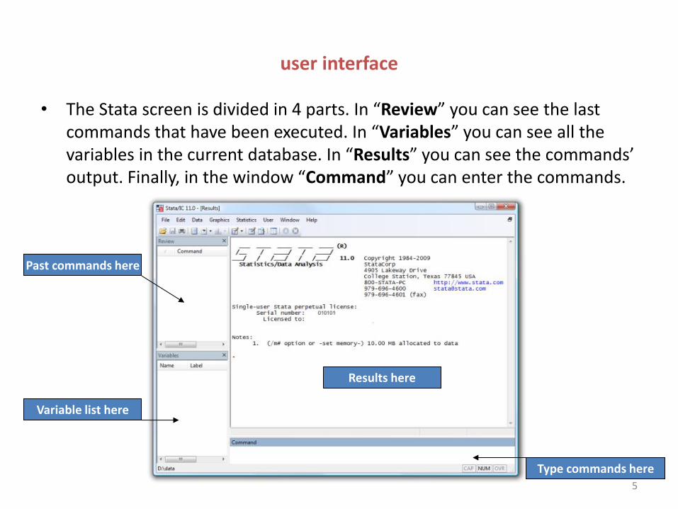
• The Stata screen is divided in 4 parts. In “Review” you can see the last commands that have been executed. In “Variables” you can see all the variables in the current database. In “Results” you can see the commands’ output. Finally, in the window “Command” you can enter the commands.

Results here

Past commands here

Variable list here

Type commands here

6

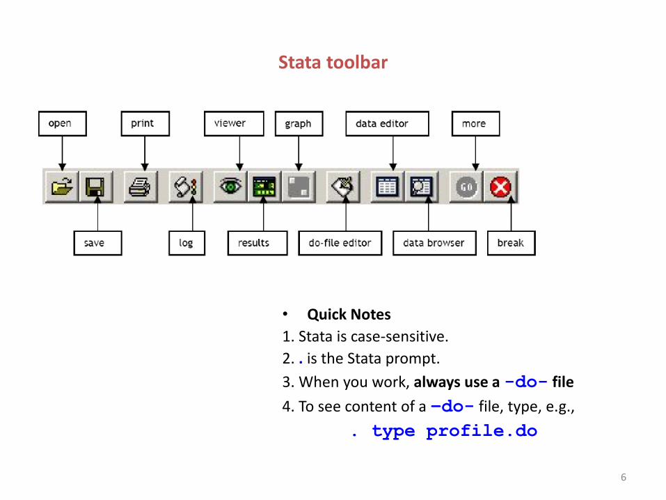
Stata toolbar

• Quick Notes

1. Stata is case-sensitive.

2. . is the Stata prompt.

3. When you work, always use a -do- file

4. To see content of a –do- file, type, e.g.,

. type profile.do

7

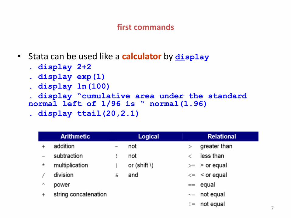
first commands

• Stata can be used like a calculator by display . display 2+2

. display exp(1)

. display ln(100)

. display “cumulative area under the standard normal left of 1/96 is “ normal(1.96)

. display ttail(20,2.1)

8

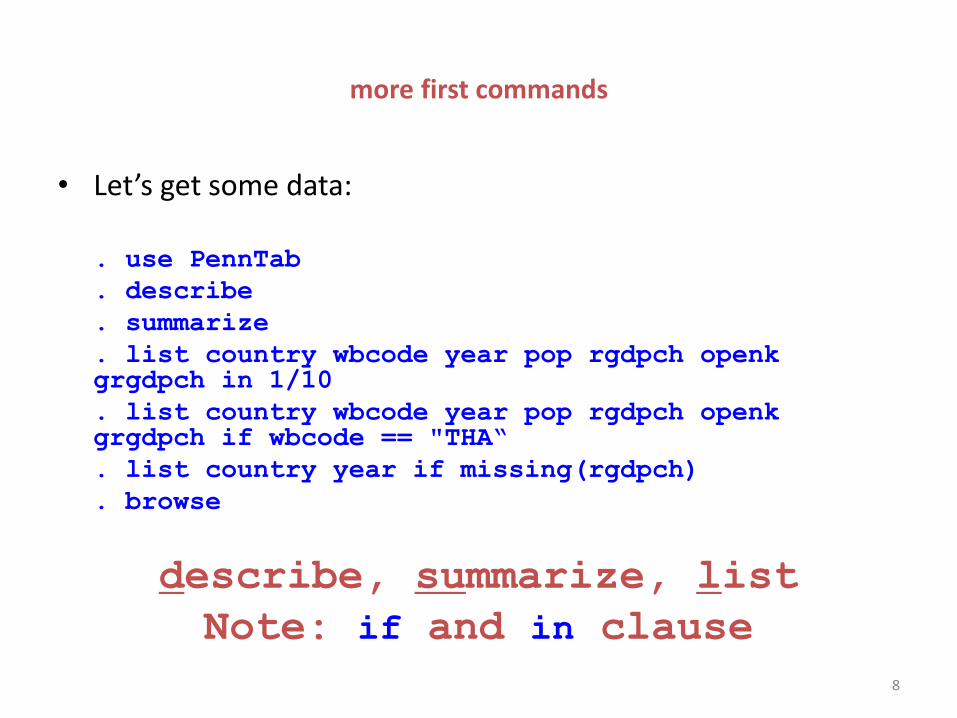
more first commands

• Let’s get some data:

. use PennTab

. describe

. summarize

. list country wbcode year pop rgdpch openk grgdpch in 1/10

. list country wbcode year pop rgdpch openk grgdpch if wbcode == "THA“

. list country year if missing(rgdpch)

. browse

describe, summarize, list

Note: if and in clause

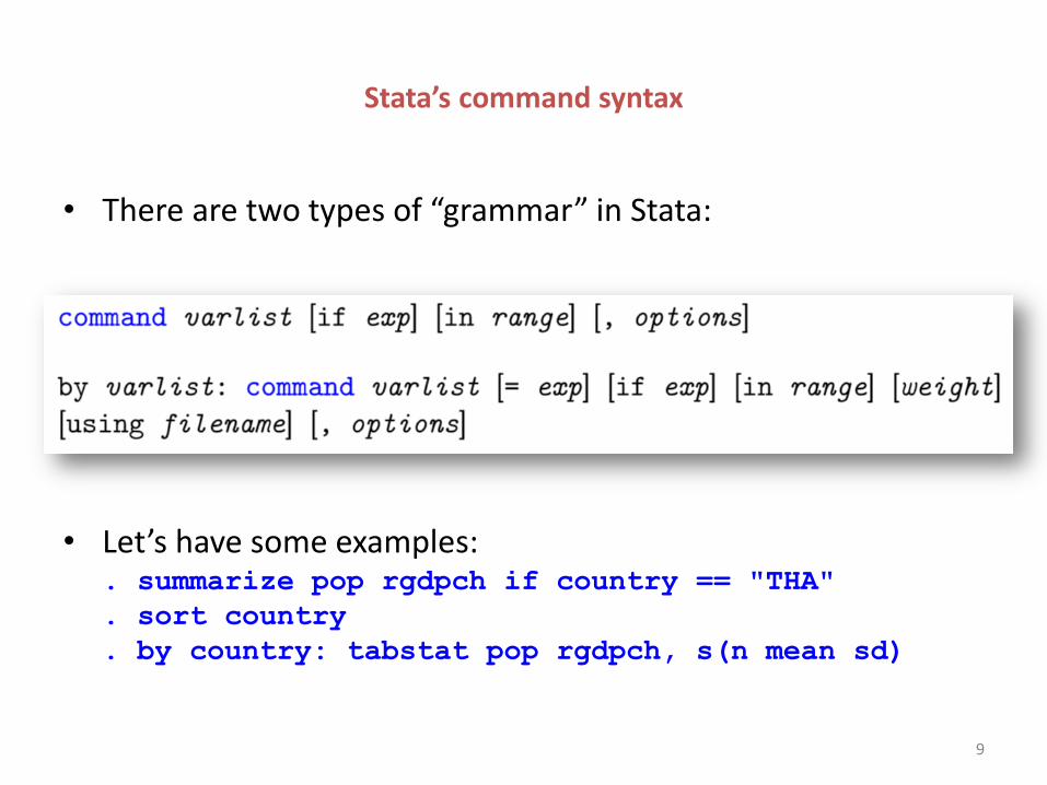
Stata’s command syntax

• There are two types of “grammar” in Stata:

• Let’s have some examples: . summarize pop rgdpch if country == "THA"

. sort country

. by country: tabstat pop rgdpch, s(n mean sd)

9

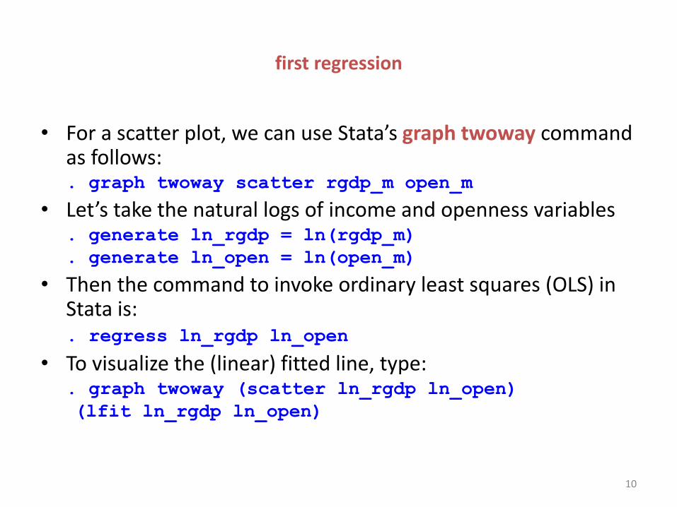
first regression

• For a scatter plot, we can use Stata’s graph twoway command as follows:

. graph twoway scatter rgdp_m open_m

• Let’s take the natural logs of income and openness variables . generate ln_rgdp = ln(rgdp_m)

. generate ln_open = ln(open_m)

• Then the command to invoke ordinary least squares (OLS) in Stata is:

. regress ln_rgdp ln_open

• To visualize the (linear) fitted line, type: . graph twoway (scatter ln_rgdp ln_open)

(lfit ln_rgdp ln_open)

10

11

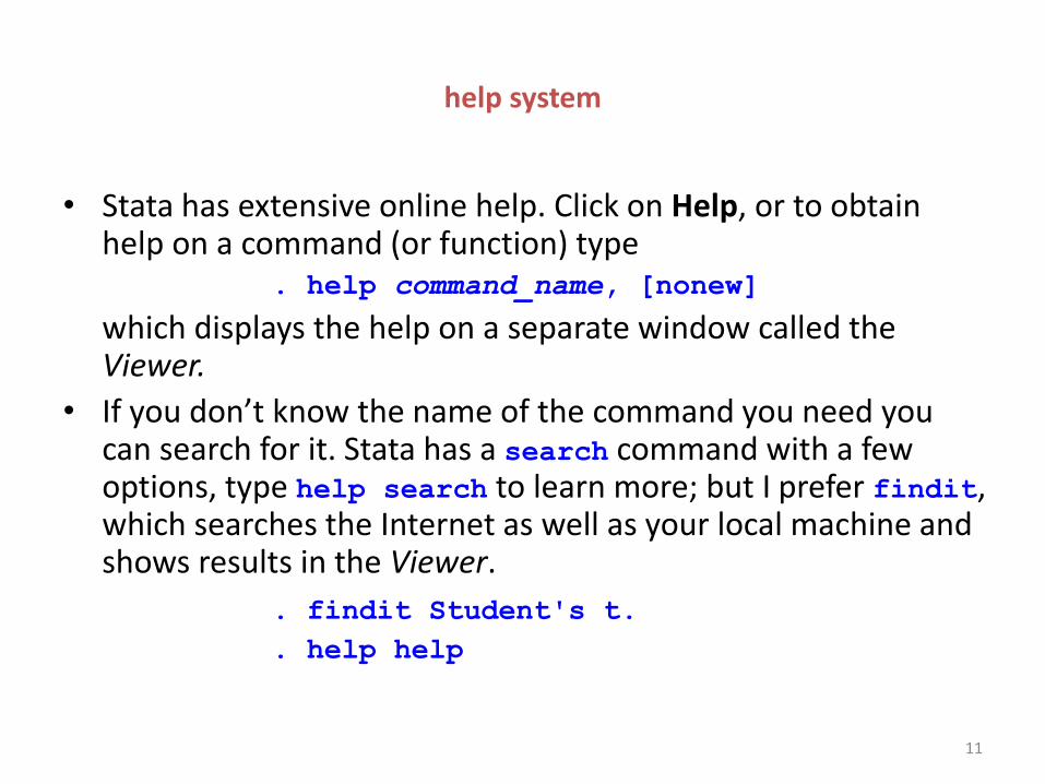
help system

• Stata has extensive online help. Click on Help, or to obtain help on a command (or function) type

. help command_name, [nonew]

which displays the help on a separate window called the Viewer.

• If you don’t know the name of the command you need you can search for it. Stata has a search command with a few options, type help search to learn more; but I prefer findit, which searches the Internet as well as your local machine and shows results in the Viewer.

. findit Student's t.

. help help

12

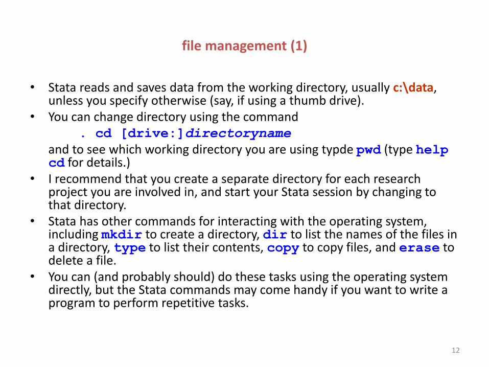
file management (1)

• Stata reads and saves data from the working directory, usually c:\data, unless you specify otherwise (say, if using a thumb drive).

• You can change directory using the command . cd [drive:]directoryname

and to see which working directory you are using typde pwd (type help cd for details.)

• I recommend that you create a separate directory for each research project you are involved in, and start your Stata session by changing to that directory.

• Stata has other commands for interacting with the operating system, including mkdir to create a directory, dir to list the names of the files in a directory, type to list their contents, copy to copy files, and erase to delete a file.

• You can (and probably should) do these tasks using the operating system directly, but the Stata commands may come handy if you want to write a program to perform repetitive tasks.

13

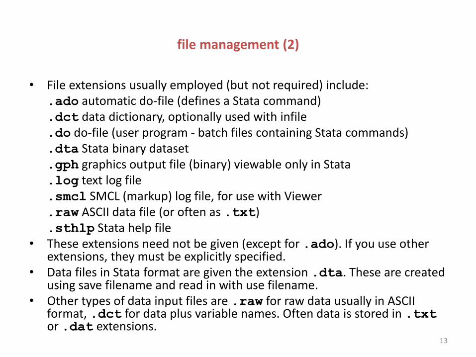
file management (2)

• File extensions usually employed (but not required) include: .ado automatic do-file (defines a Stata command) .dct data dictionary, optionally used with infile .do do-file (user program - batch files containing Stata commands) .dta Stata binary dataset .gph graphics output file (binary) viewable only in Stata .log text log file .smcl SMCL (markup) log file, for use with Viewer .raw ASCII data file (or often as .txt) .sthlp Stata help file • These extensions need not be given (except for .ado). If you use other

extensions, they must be explicitly specified. • Data files in Stata format are given the extension .dta. These are created

using save filename and read in with use filename. • Other types of data input files are .raw for raw data usually in ASCII

format, .dct for data plus variable names. Often data is stored in .txt or .dat extensions.

14

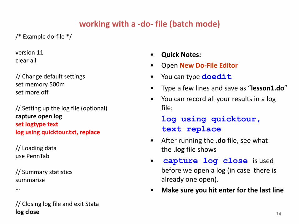
working with a -do- file (batch mode)

/* Example do-file */ version 11 clear all // Change default settings set memory 500m set more off // Setting up the log file (optional) capture open log set logtype text log using quicktour.txt, replace // Loading data use PennTab // Summary statistics summarize … // Closing log file and exit Stata log close

• Quick Notes:

• Open New Do-File Editor

• You can type doedit

• Type a few lines and save as “lesson1.do”

• You can record all your results in a log file:

log using quicktour,

text replace

• After running the .do file, see what the .log file shows

• capture log close is used

before we open a log (in case there is already one open).

• Make sure you hit enter for the last line

15

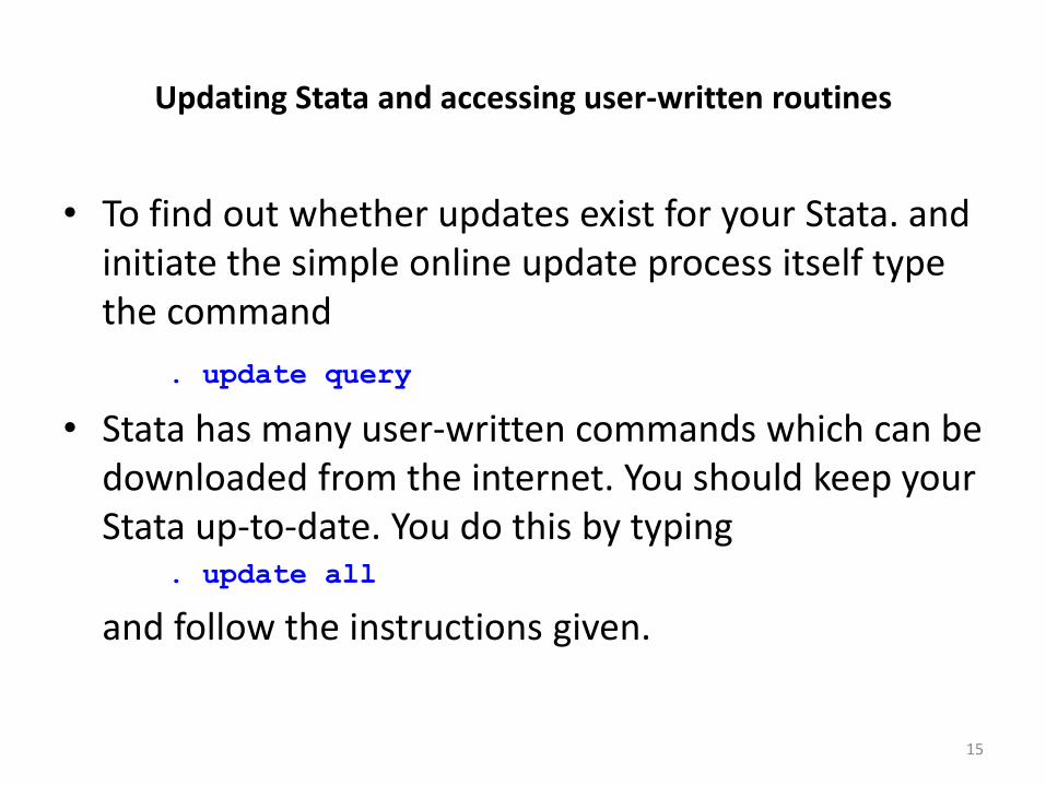
Updating Stata and accessing user-written routines

• To find out whether updates exist for your Stata. and initiate the simple online update process itself type the command

. update query

• Stata has many user-written commands which can be downloaded from the internet. You should keep your Stata up-to-date. You do this by typing

. update all

and follow the instructions given.

accessing user-written routines

• Stata native graph types are not ideal for viewing categorical-variable distributions and histograms. In this case, for example, it is nice to employ the user-written program called catplot, which you can obtain by typing:

. findit catplot

• Simply follow the links to install. Then try: . catplot income_grp percent

. catplot rgdp_m, percent by(income_grp)

• There are many specially written (by Stata and by independent authors) commands and routines you can use, easily found over the web.

• You can even get Stata data online (e.g. Penn Tables, World Bank data, etc.)

16

comments and annotations

• Comments can be written on a line starting with // or * (the line is ignored).

• // can be used at the beginning or end of a line (must be preceded by one or more blanks if at the end); everything on the line after // is ignored.

• You can also put long comments inside these /* */ to block comment them out (everything between /* and */ is ignored).

• You can continue a line in a -do- file using ///. This instructs Stata to join the next line following from /// with the current line; this must be preceded by one or more blanks; It is essentially used make long lines more readable.

• Stating #delimit ; allows you to end lines with ;

• To terminate this command type #delimit cr

17

18

Data management: basic principles of organization and transformation

• Stata is an excellent tool for data management and manipulation: moving data from external sources into the program, cleaning it up, generating new variables, generating summary data sets, merging data sets and checking for merge errors, collapsing cross–section time-series data on either of its dimensions, reshaping data sets from “long” to “wide”, and so on.

• In this context, Stata is an excellent program for answering ad hoc questions about any aspect of the data.

19

variable types

• Stata recognizes two types of variables: string and numeric. Subsequently, each variable can be stored in a number of storage types (byte, int, long; float, and double for numeric variables and str1 to str224 for string variables).

• If you have a string variable and you need to generate numeric codes, you may find useful the command encode. For instance, consider a variable "name" that takes the value "Nick" for the observations belonging to Nick, "John" for the observations belonging to John, and so forth. Then you may find useful the following:

. encode name, gen(code)

• A numeric code-variable will be generated (e.g. it takes the value 1 for the observations belonging to Nick, the value 2 for the observations belonging to John, and so forth).

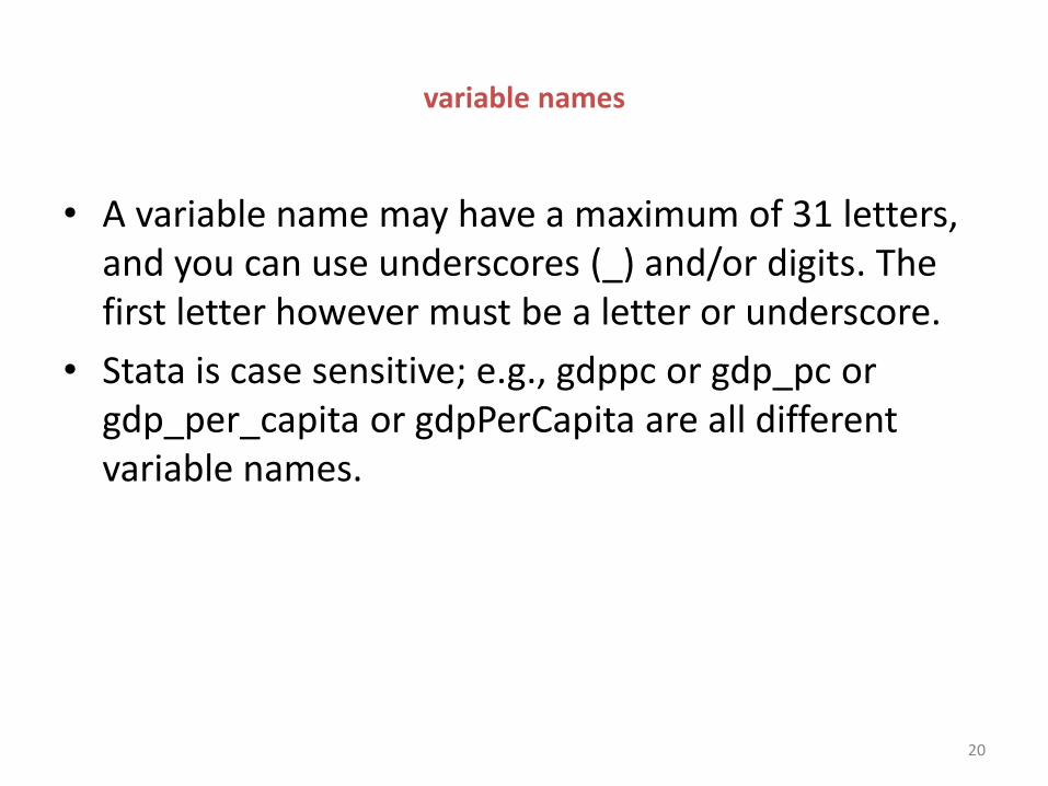
variable names

• A variable name may have a maximum of 31 letters, and you can use underscores (_) and/or digits. The first letter however must be a letter or underscore.

• Stata is case sensitive; e.g., gdppc or gdp_pc or gdp_per_capita or gdpPerCapita are all different variable names.

20

21

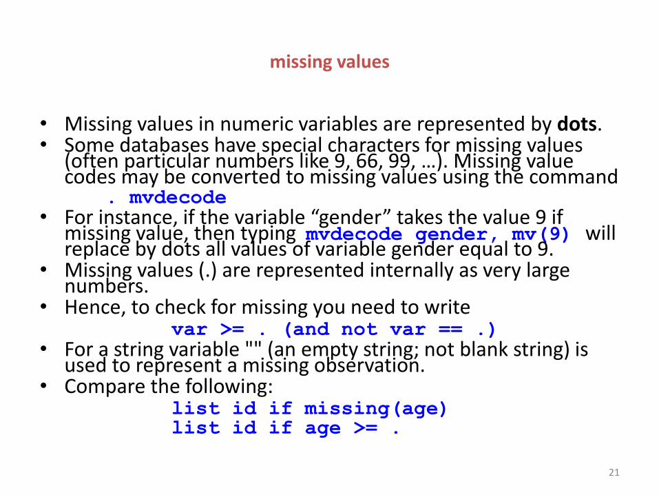
missing values

• Missing values in numeric variables are represented by dots. • Some databases have special characters for missing values

(often particular numbers like 9, 66, 99, …). Missing value codes may be converted to missing values using the command

. mvdecode • For instance, if the variable “gender” takes the value 9 if

missing value, then typing mvdecode gender, mv(9) will replace by dots all values of variable gender equal to 9.

• Missing values (.) are represented internally as very large numbers.

• Hence, to check for missing you need to write var >= . (and not var == .) • For a string variable "" (an empty string; not blank string) is

used to represent a missing observation. • Compare the following: list id if missing(age) list id if age >= .

observation subscripts _n and _N

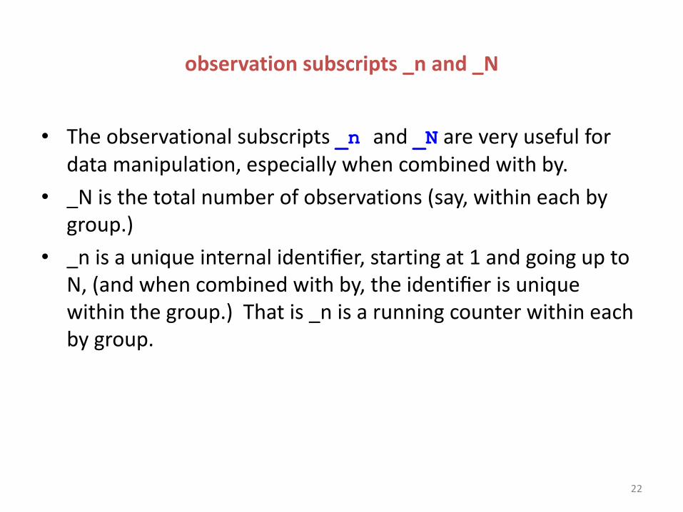
• The observational subscripts _n and _N are very useful for data manipulation, especially when combined with by.

• _N is the total number of observations (say, within each by group.)

• _n is a unique internal identifier, starting at 1 and going up to N, (and when combined with by, the identifier is unique within the group.) That is _n is a running counter within each by group.

22

making categorical variable

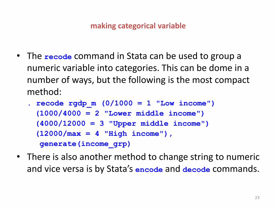
• The recode command in Stata can be used to group a numeric variable into categories. This can be dome in a number of ways, but the following is the most compact method:

. recode rgdp_m (0/1000 = 1 "Low income")

(1000/4000 = 2 "Lower middle income")

(4000/12000 = 3 "Upper middle income")

(12000/max = 4 "High income"),

generate(income_grp)

• There is also another method to change string to numeric and vice versa is by Stata’s encode and decode commands.

23

24

loading data (1)

• Comma-separated (CSV) files or tab-delimited data files may be read very easily with the insheet command—which despite its name does not read spreadsheet files. If your file has variable names in the first row that are valid for Stata, they will be automatically used (rather than default variable names). You usually need not specify whether the data are tab- or comma-delimited. Note that insheet cannot read space-delimited data (or character strings with embedded spaces, unless they are quoted).

• If the file extension is .raw, you may just use . insheet using filename

to read it. If other file extensions are used, they must be given: . insheet using filename.csv

. insheet using filename.txt

25

loading data (2)

• A free-format ASCII text file with space-, tab-, or comma-delimited data may be read with the infile command. The missing-data indicator (.) may be used to specify that values are missing.

• The command must specify the variable names. Assuming divorce.raw contains string and numeric data, to load this type

. infile str45 country gdppc d_rate grwth

using divorce.raw, clear

• Note str45 would read up to a maximum 45-letter country of origin and the number of observations will be determined from the available data.

26

loading data (3)

• The infile command may also be used with fixed-format data, including data containing undelimited string variables, by creating a dictionary file which describes the format of each variable and specifies where the data are to be found. The dictionary may also specify that more than one record in the input file corresponds to a single observation in the data set.

• If data fields are not delimited—for instance, if the sequence ‘102’ should actually be considered as three integer variables. A dictionary must be used to define the variables’ locations. The byvariable() option allows a variable-wise dataset to be read, where one specifies the number of observations available for each series.

• An alternative to infile with a dictionary is the infix command, which presents a syntax similar to that used by SAS for the definition of variables’ data types and locations in a fixed-format ASCII data set: that is, a data file in which certain columns contain certain variables. The _column() directive allow contents of a fixed-format data file to be retrieved selectively. infix may also be used for more complex record layouts where one individual’s data are contained on several records in an ASCII file.

27

loading data (4)

• A logical condition may be used on the infile or infix commands to read only those records for which certain conditions are satisfied: i.e.

. infix using employee if sex=="M"

. infile price mpg using auto in 1/20

where the latter will read only the first 20 observations from the external file. This might be very useful when reading a large data set, where one can check to see that the formats are being properly specified on a subset of the file.

• If your data are already in the internal format of SAS, SPSS, Excel, GAUSS, MATLAB, or a number of other packages, the best way to get it into Stata is by using the third-party product StatTransfer. StatTransfer will preserve variable labels, value labels, and other aspects of the data, and can be used to convert a Stata binary file into other packages’ formats.

28

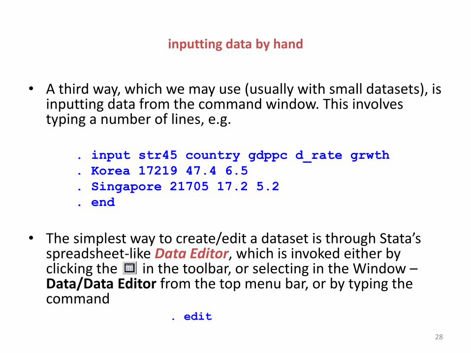
inputting data by hand

• A third way, which we may use (usually with small datasets), is inputting data from the command window. This involves typing a number of lines, e.g.

. input str45 country gdppc d_rate grwth

. Korea 17219 47.4 6.5

. Singapore 21705 17.2 5.2

. end

• The simplest way to create/edit a dataset is through Stata’s

spreadsheet-like Data Editor, which is invoked either by clicking the in the toolbar, or selecting in the Window – Data/Data Editor from the top menu bar, or by typing the command

. edit

29

creating a new dataset

• If you want to save (as a Stata data file), simply type . save filename, replace

• Saving a file as a Stata .dta file is useful, and calling it is especially easy; Just type

. use filename, clear

• If however you want save your data as an ASCII file, type . outsheet using filename.txt, replace

• If you do not specify an extension (e.g. .txt or .csv, comma

for comma separated variable data files), Stata automatically save your data as an extension .raw ASCII file.

30

sorting (and merging/combining datasets)

• The sort command arranges the observations of the current data into ascending order. This command is particularly useful in two situations.

• Stata has a more powerful sort command gsort. • 1. When using the by varlist: prefix (discussed before) data must

be sorted by varlist, i.e. . sort region

. by region: summarize gnppc • 2. When merging datasets, the data must be sorted by so that

observations can be uniquely identified so that the merge command can match observations correctly, i.e.

. use dataset1

. sort id

. merge 1:1 id using dataset2 • 3. To combine datasets, use the append command: . use dataset1

. append using dataset2

31

creating, editing, renaming (new) variables

• The generate command is often used to create a new variable. For example,

. generate male_d = male==1 & !missing(male)

. gen agegrp = ”young” if age<18

• To change the contents of an existing variable you must use the replace command, i.e.

. replace variable = expression

• To change variable names simply use the rename command. i.e. . rename old_name new_name

• To help keep track of variables, it is useful to use the labels command, e.g.,

. label data “Divorce Data: 2002”

. label variable d_rate “Divorce Rate”

32

Introduction to graphics

• Stata graphics are excellent tools for exploratory data analysis, and can produce high-quality 2-D publication-quality graphics in several dozen different forms. Every aspect of graphics may be programmed and customized, and new graph types and graph “schemes” are being continuously developed. The programmability of graphics implies that a number of similar graphs may be generated without any “pointing and clicking” to alter aspects of the graphs.

• You have already seen an example in your first –do- file.

33

Producing publication-quality output

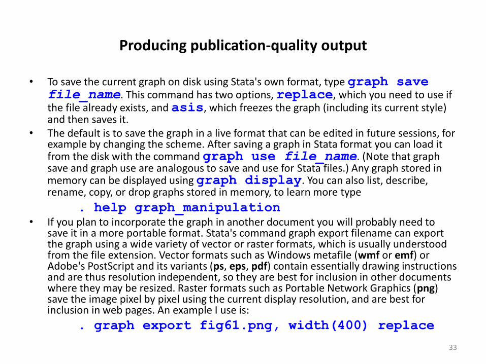
• To save the current graph on disk using Stata's own format, type graph save file_name. This command has two options, replace, which you need to use if the file already exists, and asis, which freezes the graph (including its current style) and then saves it.

• The default is to save the graph in a live format that can be edited in future sessions, for example by changing the scheme. After saving a graph in Stata format you can load it from the disk with the command graph use file_name. (Note that graph save and graph use are analogous to save and use for Stata files.) Any graph stored in memory can be displayed using graph display. You can also list, describe, rename, copy, or drop graphs stored in memory, to learn more type

. help graph_manipulation • If you plan to incorporate the graph in another document you will probably need to

save it in a more portable format. Stata's command graph export filename can export the graph using a wide variety of vector or raster formats, which is usually understood from the file extension. Vector formats such as Windows metafile (wmf or emf) or Adobe's PostScript and its variants (ps, eps, pdf) contain essentially drawing instructions and are thus resolution independent, so they are best for inclusion in other documents where they may be resized. Raster formats such as Portable Network Graphics (png) save the image pixel by pixel using the current display resolution, and are best for inclusion in web pages. An example I use is:

. graph export fig61.png, width(400) replace

34

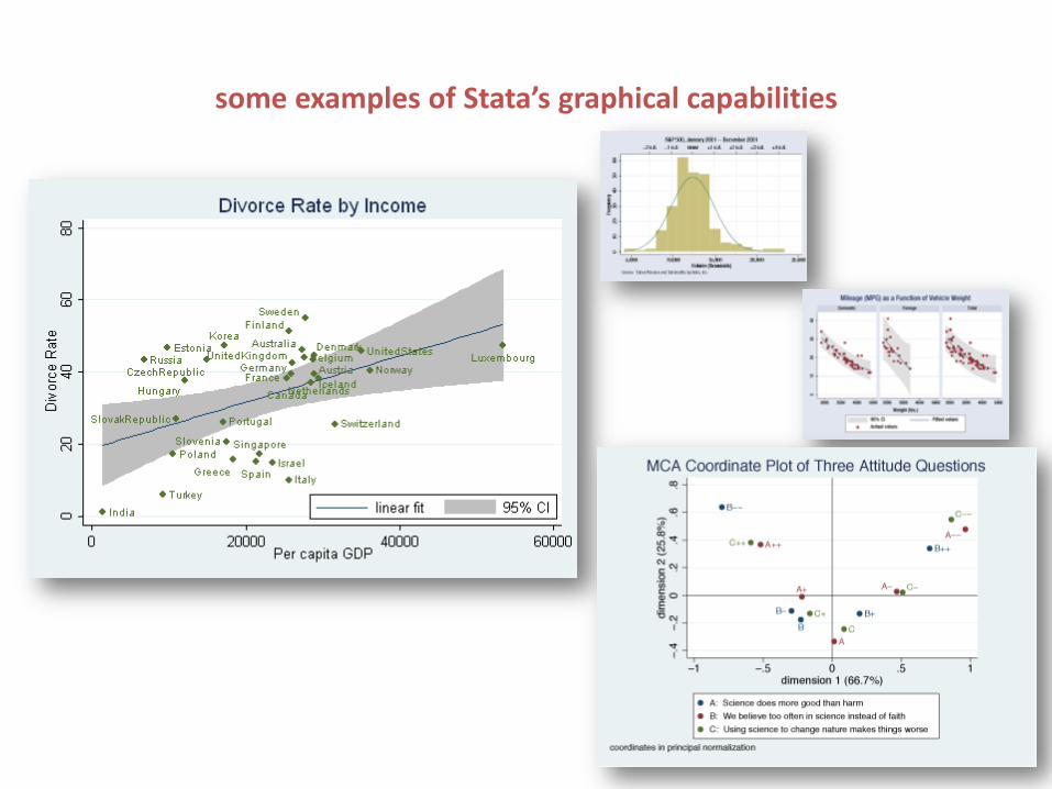
some examples of Stata’s graphical capabilities

35

seven basic types of graphs

. histogram histograms

. graph twoway two-variable scatterplots, line plots, and many others . graph matrix scatterplot matrices

. graph box box plots

. graph pie pie charts

. graph bar bar charts

. graph dot dot plots • We will mainly make use of graph twoway

36

fitting lines

• To produce a simple scatter plot of two variables, use the command . graph twoway scatter ln_rgdp ln_open

• To show the fitted regression line as well, we use lfit (qfit is used for quadratic fit). . graph twoway (lfitci ln_rgdp ln_open) (scatter ln_rgdp ln_open), title(“Openness and Economic Development: 1990-2004”)

• To label the points using text included in another variable, we can use the mlabel(varname) option. For example, we add the country names to the plot: . graph twoway (lfitci ln_rgdp ln_open, legend(off)) (scatter ln_rgdp ln_open, mlabel(country))

• legend(off) hides the legend.

37

tidying up labels

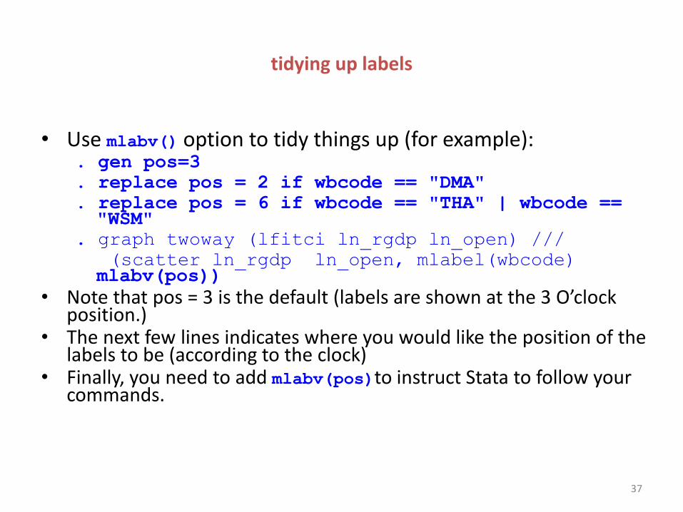
• Use mlabv() option to tidy things up (for example): . gen pos=3

. replace pos = 2 if wbcode == "DMA"

. replace pos = 6 if wbcode == "THA" | wbcode == "WSM"

. graph twoway (lfitci ln_rgdp ln_open) ///

(scatter ln_rgdp ln_open, mlabel(wbcode) mlabv(pos))

• Note that pos = 3 is the default (labels are shown at the 3 O’clock position.)

• The next few lines indicates where you would like the position of the labels to be (according to the clock)

• Finally, you need to add mlabv(pos)to instruct Stata to follow your commands.

38

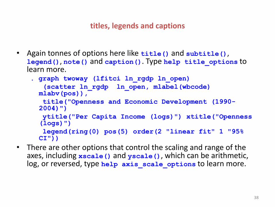
titles, legends and captions

• Again tonnes of options here like title() and subtitle(), legend(), note() and caption(). Type help title_options to learn more. . graph twoway (lfitci ln_rgdp ln_open)

(scatter ln_rgdp ln_open, mlabel(wbcode) mlabv(pos)),

title("Openness and Economic Development (1990-2004)")

ytitle("Per Capita Income (logs)") xtitle("Openness (logs)")

legend(ring(0) pos(5) order(2 "linear fit" 1 "95% CI"))

• There are other options that control the scaling and range of the axes, including xscale() and yscale(), which can be arithmetic, log, or reversed, type help axis_scale_options to learn more.

Part 2

• Regression Basics (with Stata) – Inference and the idea of sampling distribution

– Regression: Estimation and inference

– OLS assumptions and properties

– Post-estimation regression diagnosis: Violating the classical assumptions (consequences, detection, solution)

– The problem of endogeniety again!

39

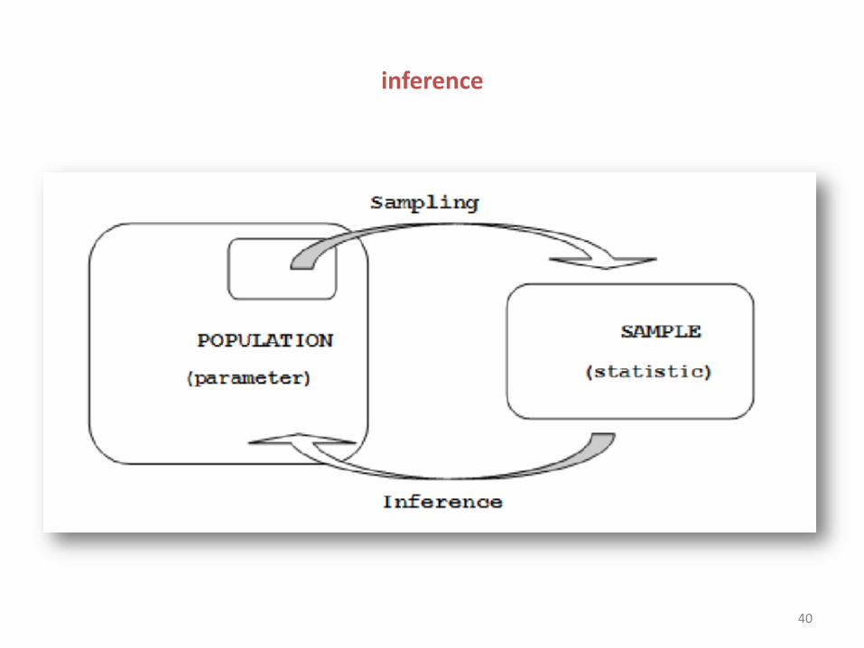
inference

40

simple random sample

• As statisticians we would like to know some characteristic (parameter) of a population of interest. To do so, we usually take a sample, calculate some statistic which is used to estimate the population parameter.

• - The most basic type of sample is the Simple Random Sample (SRS), which will serve as our reference point for most of the discussion that follows.

• In a SRS, each possible sample of the population of size n has an equal probability of being chosen as the sample.

41

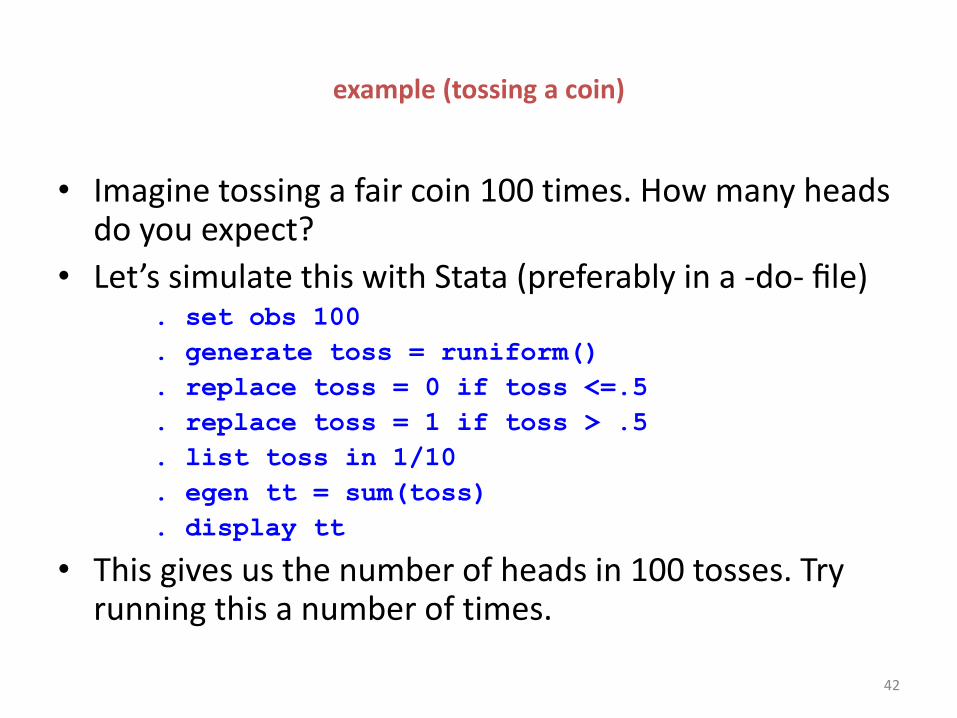
example (tossing a coin)

• Imagine tossing a fair coin 100 times. How many heads do you expect?

• Let’s simulate this with Stata (preferably in a -do- file) . set obs 100

. generate toss = runiform()

. replace toss = 0 if toss <=.5

. replace toss = 1 if toss > .5

. list toss in 1/10

. egen tt = sum(toss)

. display tt

• This gives us the number of heads in 100 tosses. Try running this a number of times.

42

43

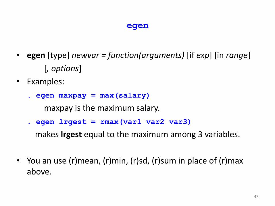
egen

• egen [type] newvar = function(arguments) [if exp] [in range]

[, options]

• Examples:

. egen maxpay = max(salary)

maxpay is the maximum salary.

. egen lrgest = rmax(var1 var2 var3)

makes lrgest equal to the maximum among 3 variables.

• You an use (r)mean, (r)min, (r)sd, (r)sum in place of (r)max above.

44

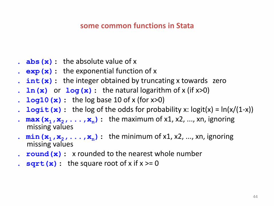
some common functions in Stata

. abs(x): the absolute value of x

. exp(x): the exponential function of x

. int(x): the integer obtained by truncating x towards zero

. ln(x) or log(x): the natural logarithm of x (if x>0)

. log10(x): the log base 10 of x (for x>0)

. logit(x): the log of the odds for probability x: logit(x) = ln(x/(1-x))

. max(x1,x2,...,xn): the maximum of x1, x2, ..., xn, ignoring missing values

. min(x1,x2,...,xn): the minimum of x1, x2, ..., xn, ignoring missing values

. round(x): x rounded to the nearest whole number

. sqrt(x): the square root of x if x >= 0

simulation in Stata

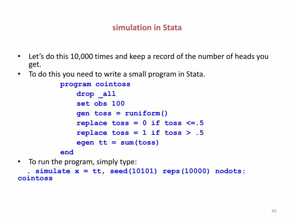
• Let’s do this 10,000 times and keep a record of the number of heads you get.

• To do this you need to write a small program in Stata. program cointoss

drop _all

set obs 100

gen toss = runiform()

replace toss = 0 if toss <=.5

replace toss = 1 if toss > .5

egen tt = sum(toss)

end

• To run the program, simply type: . simulate x = tt, seed(10101) reps(10000) nodots: cointoss

45

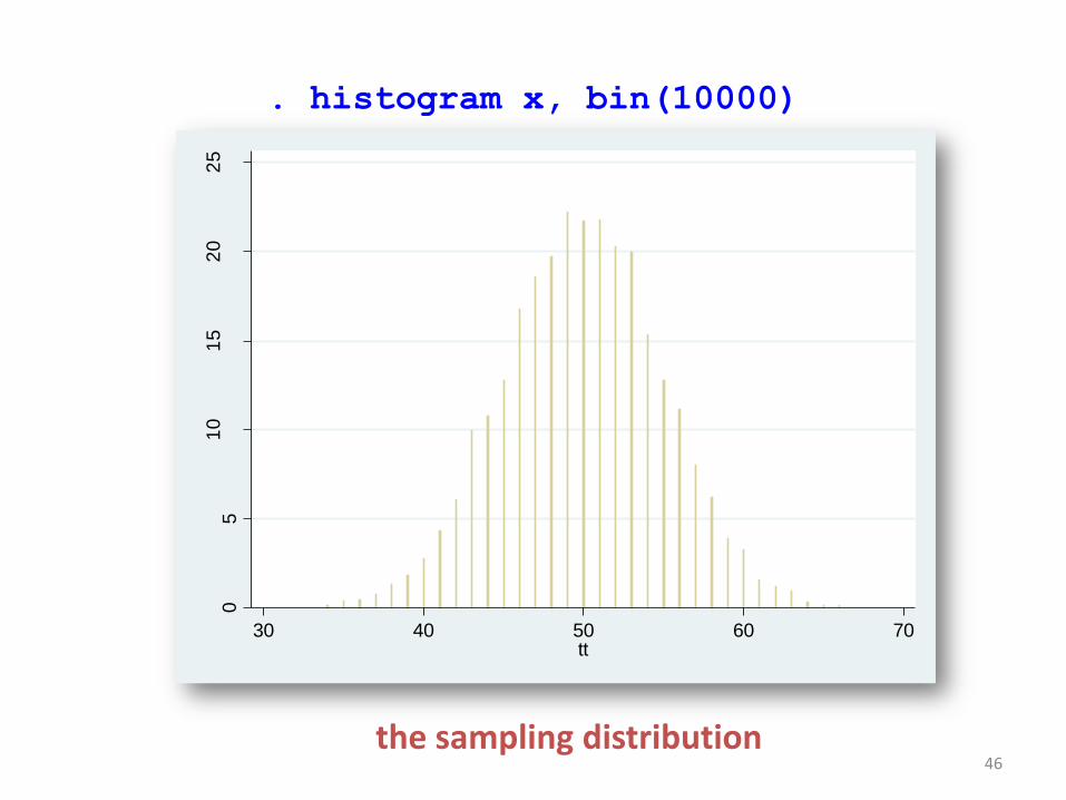
. histogram x, bin(10000)

the sampling distribution

05

10

15

20

25

Den

sity

30 40 50 60 70tt

46

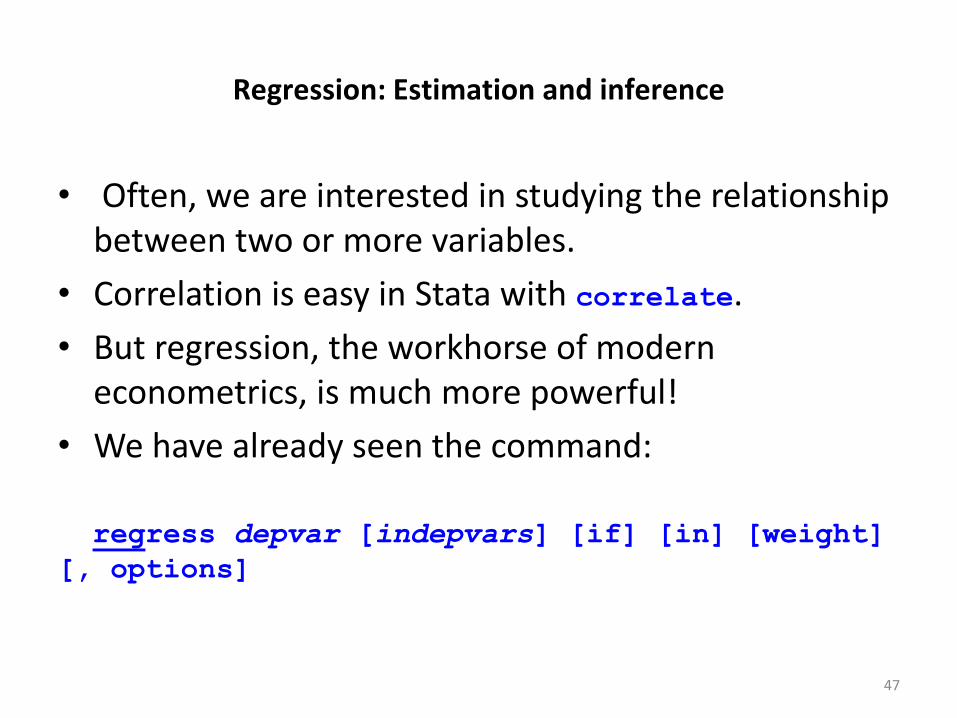
Regression: Estimation and inference

• Often, we are interested in studying the relationship between two or more variables.

• Correlation is easy in Stata with correlate.

• But regression, the workhorse of modern econometrics, is much more powerful!

• We have already seen the command:

regress depvar [indepvars] [if] [in] [weight]

[, options]

47

48

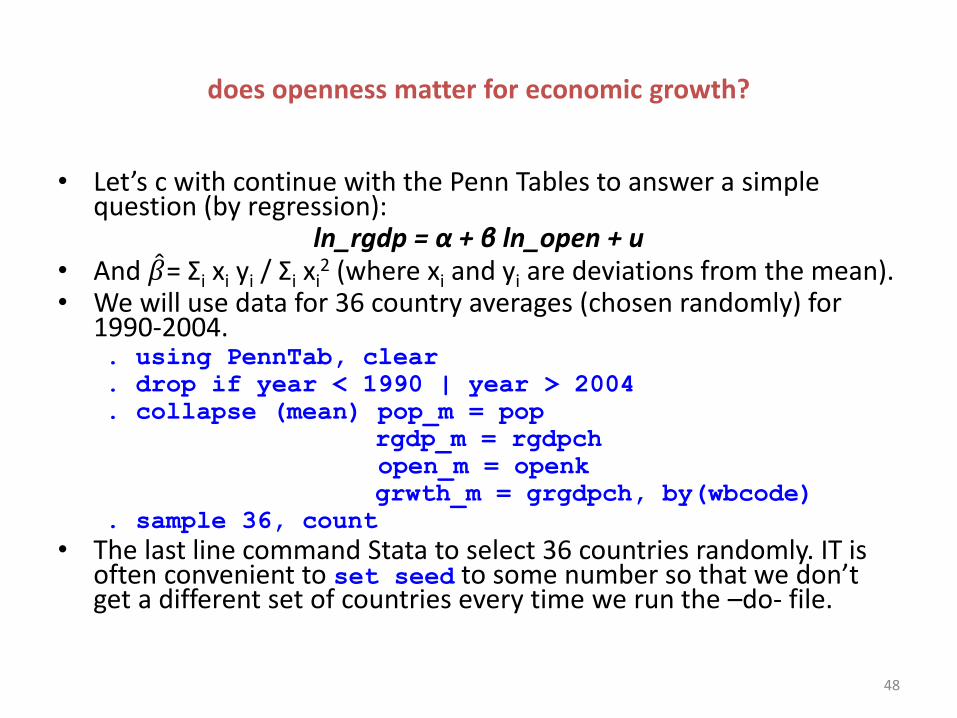
does openness matter for economic growth?

• Let’s c with continue with the Penn Tables to answer a simple question (by regression):

ln_rgdp = α + β ln_open + u • And 𝛽 = Σi xi yi / Σi xi

2 (where xi and yi are deviations from the mean). • We will use data for 36 country averages (chosen randomly) for

1990-2004. . using PennTab, clear

. drop if year < 1990 | year > 2004

. collapse (mean) pop_m = pop

rgdp_m = rgdpch

open_m = openk

grwth_m = grgdpch, by(wbcode)

. sample 36, count

• The last line command Stata to select 36 countries randomly. IT is often convenient to set seed to some number so that we don’t get a different set of countries every time we run the –do- file.

49

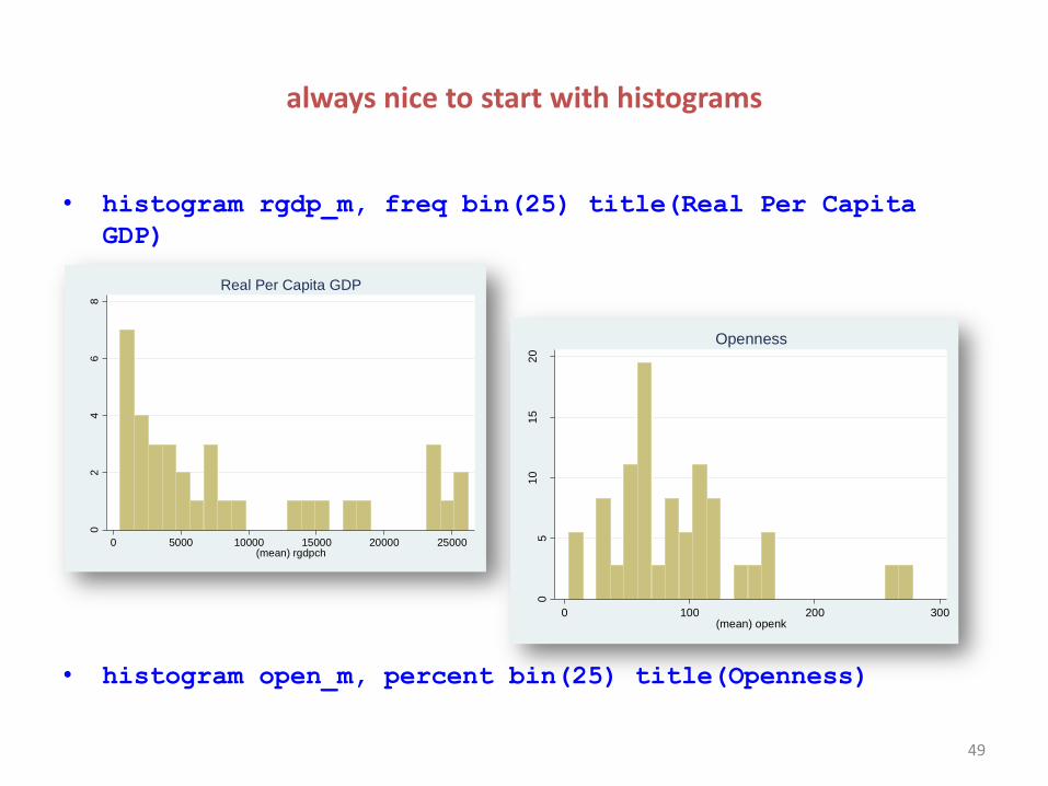
always nice to start with histograms

• histogram rgdp_m, freq bin(25) title(Real Per Capita

GDP)

• histogram open_m, percent bin(25) title(Openness)

02

46

8

Fre

que

ncy

0 5000 10000 15000 20000 25000(mean) rgdpch

Real Per Capita GDP

05

10

15

20

Pe

rcen

t

0 100 200 300(mean) openk

Openness

50

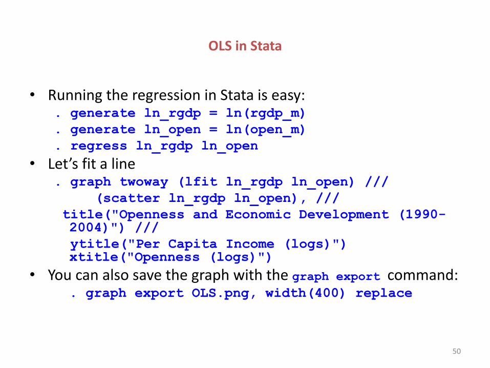
OLS in Stata

• Running the regression in Stata is easy: . generate ln_rgdp = ln(rgdp_m)

. generate ln_open = ln(open_m)

. regress ln_rgdp ln_open

• Let’s fit a line . graph twoway (lfit ln_rgdp ln_open) ///

(scatter ln_rgdp ln_open), ///

title("Openness and Economic Development (1990-2004)") ///

ytitle("Per Capita Income (logs)") xtitle("Openness (logs)")

• You can also save the graph with the graph export command: . graph export OLS.png, width(400) replace

51

lfit

BRB

LAO

WSM

PAN

THA LBN

ERI

LVA

COG

HKG

NIC

GNQ

PAK

BHS

DEU

CIV

BEN

ATG

PER

COD

ISL

AZE

NGA

RUS

MNGSYR

MEX

AUT

CUB

SOM

DMA

MAC

ECU

ESP

NLD

PRT

56

78

91

0

Pe

r C

ap

ita In

com

e (

logs)

1 2 3 4 5 6Openness (logs)

linear fit 95% CI

Openness and Economic Development (1990-2004)

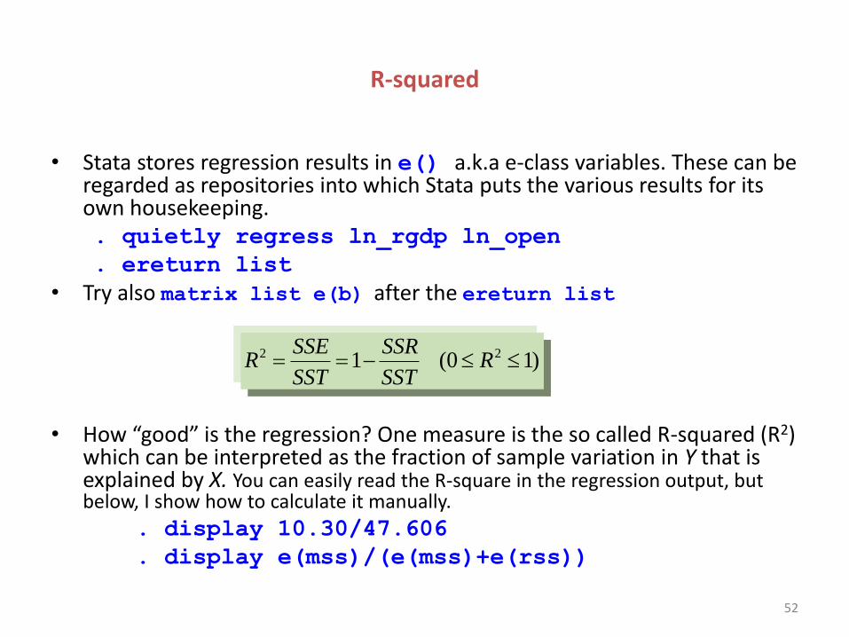
R-squared

• Stata stores regression results in e() a.k.a e-class variables. These can be regarded as repositories into which Stata puts the various results for its own housekeeping. . quietly regress ln_rgdp ln_open

. ereturn list

• Try also matrix list e(b) after the ereturn list

• How “good” is the regression? One measure is the so called R-squared (R2) which can be interpreted as the fraction of sample variation in Y that is explained by X. You can easily read the R-square in the regression output, but below, I show how to calculate it manually.

. display 10.30/47.606

. display e(mss)/(e(mss)+e(rss))

)10(1 22 RSST

SSR

SST

SSER

52

53

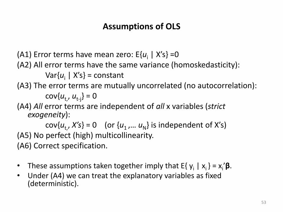
Assumptions of OLS

(A1) Error terms have mean zero: E{ui | X’s} =0 (A2) All error terms have the same variance (homoskedasticity): Var{ui | X’s} = constant (A3) The error terms are mutually uncorrelated (no autocorrelation): cov{ut,, ut-j} = 0 (A4) All error terms are independent of all x variables (strict

exogeneity): cov{ut,, X’s} = 0 (or {u1 ,… uN} is independent of X’s) (A5) No perfect (high) multicollinearity. (A6) Correct specification. • These assumptions taken together imply that E{ yi | xi } = xi’β. • Under (A4) we can treat the explanatory variables as fixed

(deterministic).

54

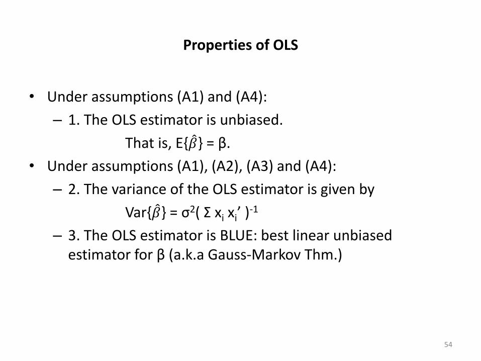
Properties of OLS

• Under assumptions (A1) and (A4):

– 1. The OLS estimator is unbiased.

That is, E{𝛽 } = β.

• Under assumptions (A1), (A2), (A3) and (A4):

– 2. The variance of the OLS estimator is given by

Var{𝛽 } = σ2( Σ xi xi’ )-1

– 3. The OLS estimator is BLUE: best linear unbiased estimator for β (a.k.a Gauss-Markov Thm.)

55

properties of OLS (2)

• Because the true (population) variance σ2 is usually unknown, we estimate this by the sampling variance of the residuals, 𝜎 2.

• Because we have k parameters when we minimize the residual sum of squares, we require a degrees of freedom correction:

𝜎 2 = (n - k)-1 Σ 𝑢 2 • Under assumptions (A1)-(A4), 𝜎 2 is an unbiased estimator

for σ2. • We estimate the variance (covariance matrix) of 𝛽 by 𝜎 2 ( Σ xi xi’ )

-1 • The square root of the kth diagonal element is the standard

error of 𝛽 k.

56

properties of OLS (3)

• A convenient assumption (that automatically replaces (A1) (A2) and (A3)) is that all error terms have a normal distribution.

ui ~ NID(0, σ2)

which is shorthand for: all ui are independent drawings from a normal distribution with mean 0 and variance σ2. (“normally and independently distributed”).

• Together with assumptions (A4), the OLS estimator 𝛽 will have a normal distribution with mean β and covariance matrix Var{𝛽 } = σ2( Σi xi xi’ )

-1.

• With non-spherical errors, we can re-specify the covariance matrix into a Generalized Least Squares (GLS) form.

57

prediction

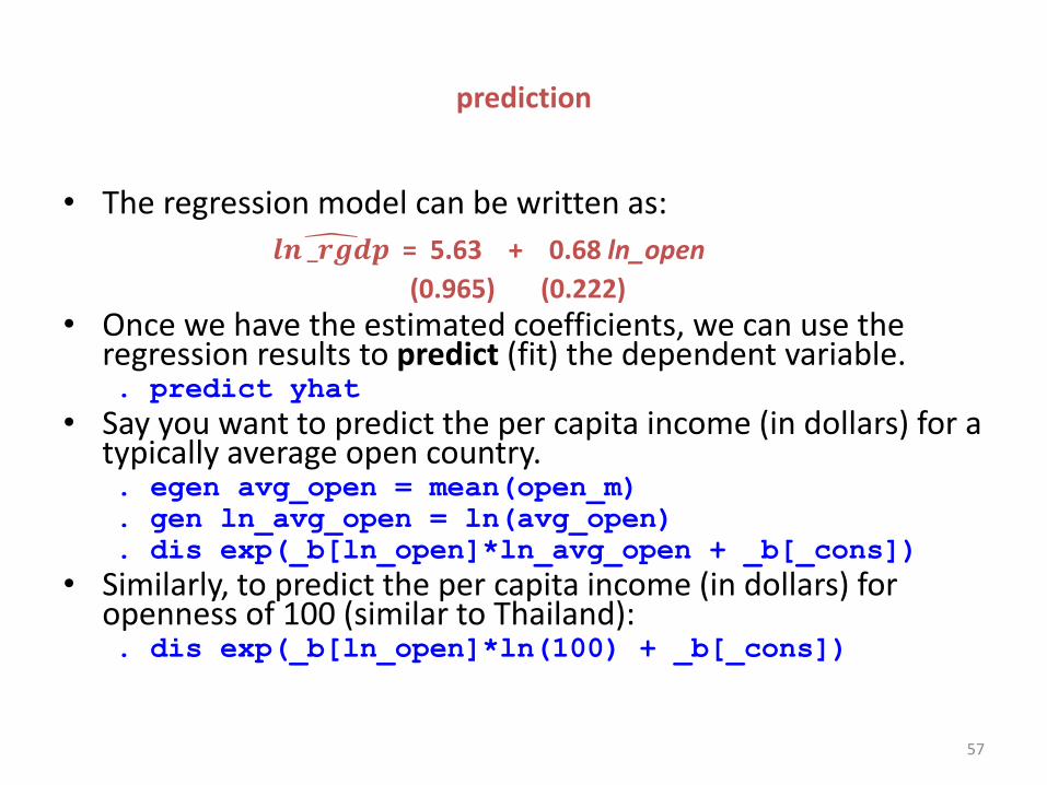
• The regression model can be written as:

𝒍𝒏 _𝒓𝒈𝒅𝒑 = 5.63 + 0.68 ln_open

(0.965) (0.222)

• Once we have the estimated coefficients, we can use the regression results to predict (fit) the dependent variable. . predict yhat

• Say you want to predict the per capita income (in dollars) for a typically average open country. . egen avg_open = mean(open_m)

. gen ln_avg_open = ln(avg_open)

. dis exp(_b[ln_open]*ln_avg_open + _b[_cons])

• Similarly, to predict the per capita income (in dollars) for openness of 100 (similar to Thailand): . dis exp(_b[ln_open]*ln(100) + _b[_cons])

58

inference

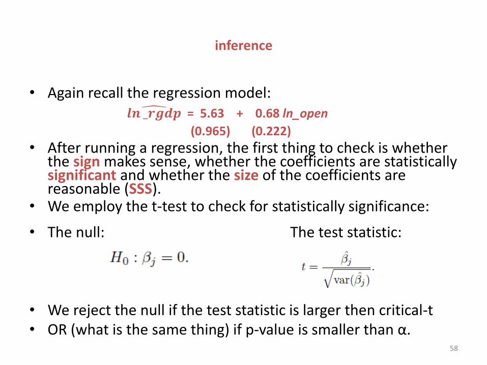
• Again recall the regression model: 𝒍𝒏 _𝒓𝒈𝒅𝒑 = 5.63 + 0.68 ln_open

(0.965) (0.222)

• After running a regression, the first thing to check is whether the sign makes sense, whether the coefficients are statistically significant and whether the size of the coefficients are reasonable (SSS).

• We employ the t-test to check for statistically significance:

• The null: The test statistic:

• We reject the null if the test statistic is larger then critical-t • OR (what is the same thing) if p-value is smaller than α.

59

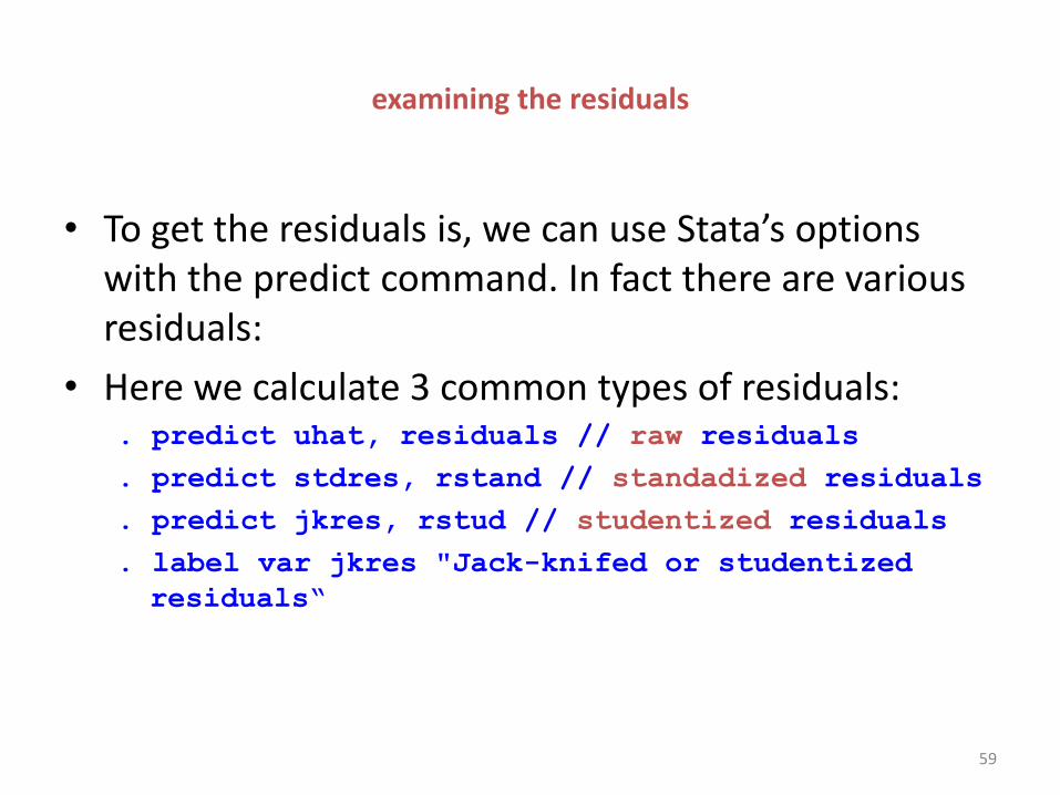
examining the residuals

• To get the residuals is, we can use Stata’s options with the predict command. In fact there are various residuals:

• Here we calculate 3 common types of residuals: . predict uhat, residuals // raw residuals

. predict stdres, rstand // standadized residuals

. predict jkres, rstud // studentized residuals

. label var jkres "Jack-knifed or studentized

residuals“

60

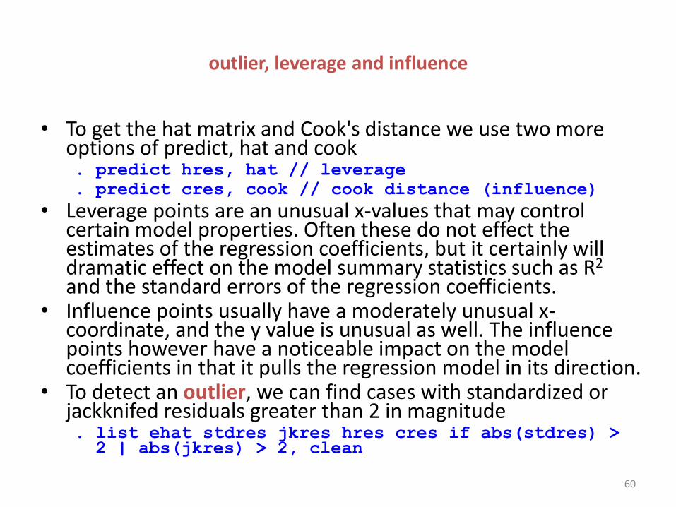
outlier, leverage and influence

• To get the hat matrix and Cook's distance we use two more options of predict, hat and cook . predict hres, hat // leverage

. predict cres, cook // cook distance (influence)

• Leverage points are an unusual x-values that may control certain model properties. Often these do not effect the estimates of the regression coefficients, but it certainly will dramatic effect on the model summary statistics such as R2 and the standard errors of the regression coefficients.

• Influence points usually have a moderately unusual x-coordinate, and the y value is unusual as well. The influence points however have a noticeable impact on the model coefficients in that it pulls the regression model in its direction.

• To detect an outlier, we can find cases with standardized or jackknifed residuals greater than 2 in magnitude . list ehat stdres jkres hres cres if abs(stdres) > 2 | abs(jkres) > 2, clean

61

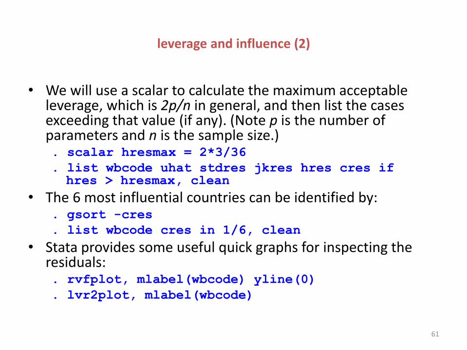
leverage and influence (2)

• We will use a scalar to calculate the maximum acceptable leverage, which is 2p/n in general, and then list the cases exceeding that value (if any). (Note p is the number of parameters and n is the sample size.) . scalar hresmax = 2*3/36

. list wbcode uhat stdres jkres hres cres if hres > hresmax, clean

• The 6 most influential countries can be identified by: . gsort -cres

. list wbcode cres in 1/6, clean

• Stata provides some useful quick graphs for inspecting the residuals: . rvfplot, mlabel(wbcode) yline(0)

. lvr2plot, mlabel(wbcode)

62

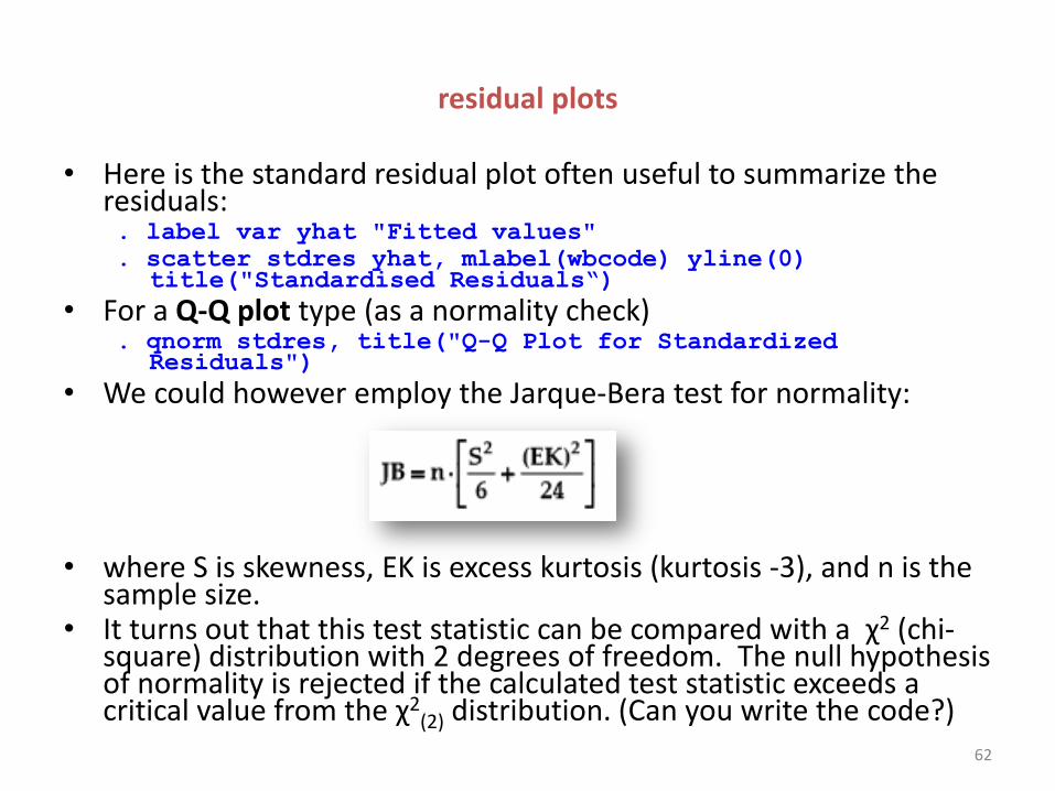
residual plots

• Here is the standard residual plot often useful to summarize the residuals: . label var yhat "Fitted values"

. scatter stdres yhat, mlabel(wbcode) yline(0) title("Standardised Residuals“)

• For a Q-Q plot type (as a normality check) . qnorm stdres, title("Q-Q Plot for Standardized

Residuals")

• We could however employ the Jarque-Bera test for normality:

• where S is skewness, EK is excess kurtosis (kurtosis -3), and n is the sample size.

• It turns out that this test statistic can be compared with a χ2 (chi-square) distribution with 2 degrees of freedom. The null hypothesis of normality is rejected if the calculated test statistic exceeds a critical value from the χ2

(2) distribution. (Can you write the code?)

63

heteroskedasticity (and autocorrelation)

• Heteroskedasticity means non-constant variances and its presence renders the usual t-test and F-tests invalid.

• Eye-balling is often not enough to detect heteroskedasticty, so a formal test is preferred. It is easy to perform a heteroskedasticity tests in Stata using the versatile estat command . estat hettest // Breusch-Pagan test

. estat imtest, white

. rvfplot, yline(0) // plots res against fitted values

• A similar problem (of unreliable standard errors) also occurs when errors are autocorrelated (usually this is commonly an issue with time series data).

• The traditional “solution” to non-constant spherical errors is to run Weighted Least Squares (WLS) or Generalized Least Squares (GLS) as opposed to OLS.

• The mnodern practice, however, and the one I recommend is that you should select the [, robust] option for all your regressions to give you the corrected (heteroskedasticity-robust standard errors) which you can use without too much worry.

64

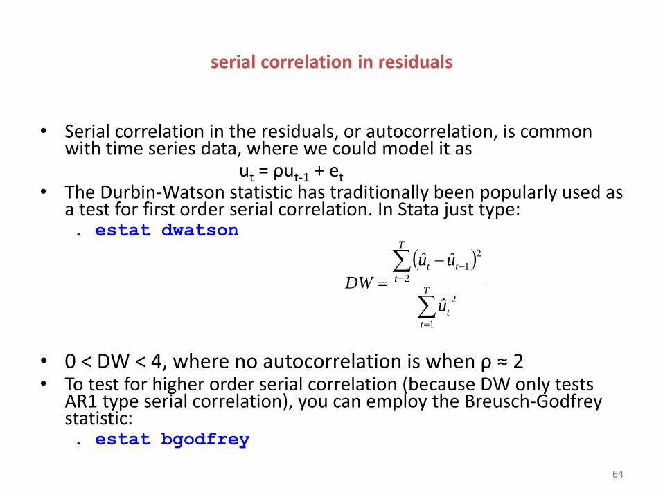
serial correlation in residuals

• Serial correlation in the residuals, or autocorrelation, is common with time series data, where we could model it as

ut = ρut-1 + et

• The Durbin-Watson statistic has traditionally been popularly used as a test for first order serial correlation. In Stata just type: . estat dwatson

• 0 < DW < 4, where no autocorrelation is when ρ ≈ 2 • To test for higher order serial correlation (because DW only tests

AR1 type serial correlation), you can employ the Breusch-Godfrey statistic: . estat bgodfrey

T

t

t

T

t

tt

u

uu

DW

1

2

2

2

1

ˆ

ˆˆ

65

the sign, significance and size (SSS), RESET and VIF

• As mentioned earlier, as a first check for any regression, you should consider the sign, significance and size (SSS) of each parameter estimate. Also take a quick look at the F-stat to verify the “overall significance of the regression” (more of this a little later).

• Ramsey’s RESET provides a rough test with the null of no specification error:

. quietly regress ln_rgdp ln_open

. estat ovtest

• Basically, after estimating the regression, it include as additional regressor squares/cubes of fitted values and checks whether they are jointly significant. If the null is rejected, nonlinear forms should be considered. That notwithstanding, the RESET does not suggest what exactly the correct alternative would be.

• For cases with more than one independent variable, you should also test for multicollinearity (MC) by typing estat vif. Values over 10 suggest problems of MC or linear dependence.

Multivariate regression

• So far we have only considered the case of a simple regression (models with one independent variable). But life is not that simple; often researchers would want to know how two or more independent variables are the influence another variable.

• We introduce multivariate regression and the gravity model. The data is a modified version from Francois, Pindyuk and Woerz (2009) consisting of trade volume in services in 2005 between various countries separated by sectors.

. use services, clear

. list exp imp trade sector dist gdp_exp gdp_imp if exp == "THA"

. list exp imp trade sector dist gdp_exp gdp_imp if imp == "THA"

66

67

68

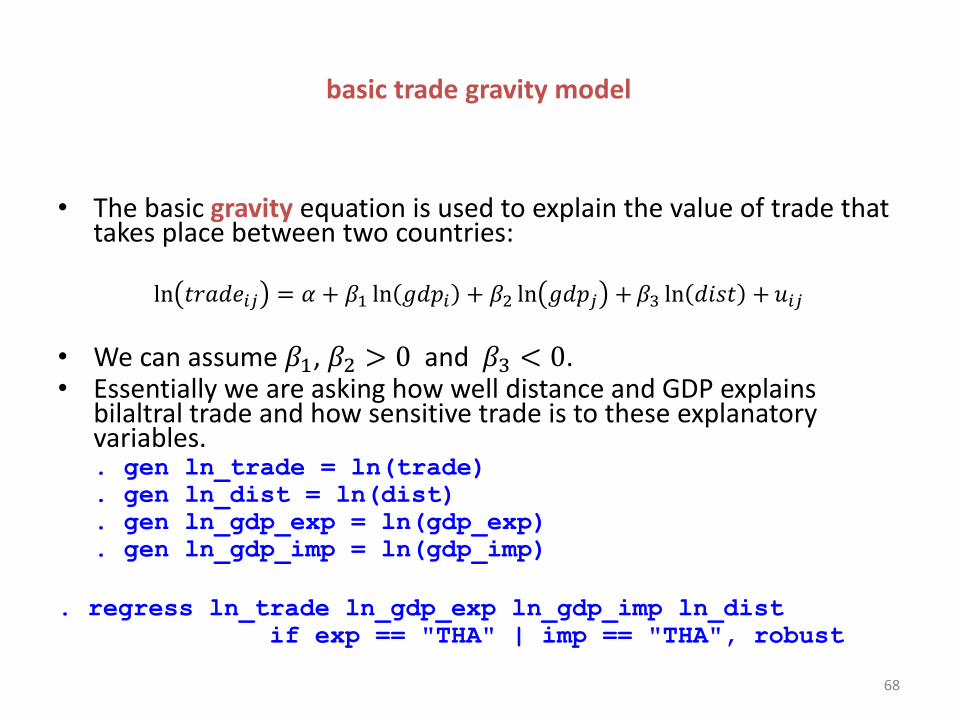
basic trade gravity model

• The basic gravity equation is used to explain the value of trade that takes place between two countries:

ln 𝑡𝑟𝑎𝑑𝑒𝑖𝑗 = 𝛼 + 𝛽1 ln 𝑔𝑑𝑝𝑖 + 𝛽2 ln 𝑔𝑑𝑝𝑗 + 𝛽3 ln 𝑑𝑖𝑠𝑡 + 𝑢𝑖𝑗

• We can assume 𝛽1, 𝛽2 > 0 and 𝛽3 < 0. • Essentially we are asking how well distance and GDP explains

bilaltral trade and how sensitive trade is to these explanatory variables.

. gen ln_trade = ln(trade)

. gen ln_dist = ln(dist)

. gen ln_gdp_exp = ln(gdp_exp)

. gen ln_gdp_imp = ln(gdp_imp)

. regress ln_trade ln_gdp_exp ln_gdp_imp ln_dist

if exp == "THA" | imp == "THA", robust

69

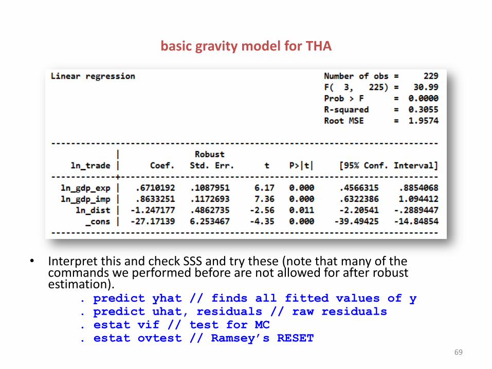
basic gravity model for THA

• Interpret this and check SSS and try these (note that many of the commands we performed before are not allowed for after robust estimation).

. predict yhat // finds all fitted values of y

. predict uhat, residuals // raw residuals

. estat vif // test for MC

. estat ovtest // Ramsey’s RESET

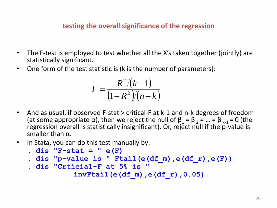
testing the overall significance of the regression

• The F-test is employed to test whether all the X’s taken together (jointly) are statistically significant.

• One form of the test statistic is (k is the number of parameters):

• And as usual, if observed F-stat > critical-F at k-1 and n-k degrees of freedom (at some appropriate α), then we reject the null of β1 = β 2 = … = β k-1 = 0 (the regression overall is statistically insignificant). Or, reject null if the p-value is smaller than α.

• In Stata, you can do this test manually by: . dis "F-stat = " e(F)

. dis "p-value is " Ftail(e(df_m),e(df_r),e(F))

. dis "Crticial-F at 5% is "

invFtail(e(df_m),e(df_r),0.05)

knR

kRF

2

2

1

1

70

71

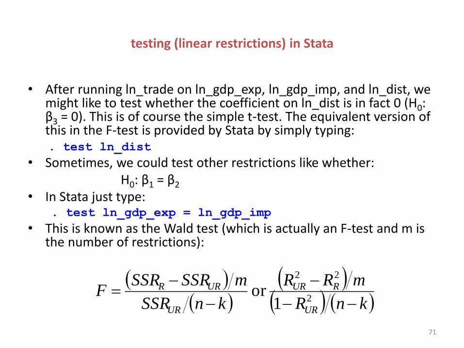
testing (linear restrictions) in Stata

• After running ln_trade on ln_gdp_exp, ln_gdp_imp, and ln_dist, we might like to test whether the coefficient on ln_dist is in fact 0 (H0: β3 = 0). This is of course the simple t-test. The equivalent version of this in the F-test is provided by Stata by simply typing:

. test ln_dist

• Sometimes, we could test other restrictions like whether: H0: β1 = β2 • In Stata just type:

. test ln_gdp_exp = ln_gdp_imp

• This is known as the Wald test (which is actually an F-test and m is the number of restrictions):

knR

mRR

knSSR

mSSRSSRF

UR

RUR

UR

URR

2

22

1or

72

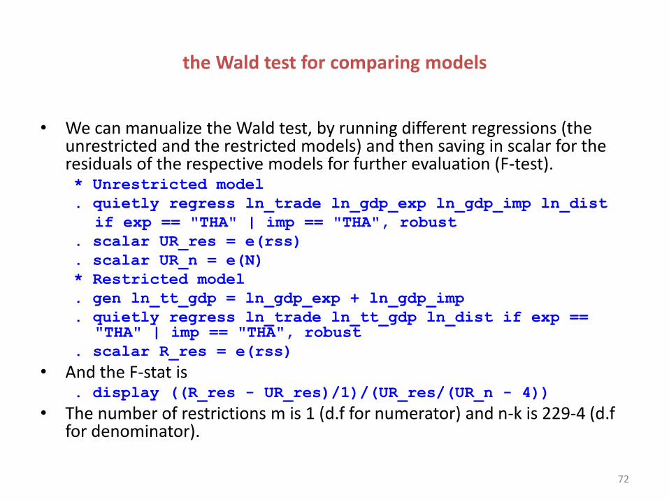
the Wald test for comparing models

• We can manualize the Wald test, by running different regressions (the unrestricted and the restricted models) and then saving in scalar for the residuals of the respective models for further evaluation (F-test). * Unrestricted model

. quietly regress ln_trade ln_gdp_exp ln_gdp_imp ln_dist

if exp == "THA" | imp == "THA", robust

. scalar UR_res = e(rss)

. scalar UR_n = e(N)

* Restricted model

. gen ln_tt_gdp = ln_gdp_exp + ln_gdp_imp

. quietly regress ln_trade ln_tt_gdp ln_dist if exp == "THA" | imp == "THA", robust

. scalar R_res = e(rss)

• And the F-stat is . display ((R_res - UR_res)/1)/(UR_res/(UR_n - 4))

• The number of restrictions m is 1 (d.f for numerator) and n-k is 229-4 (d.f for denominator).

73

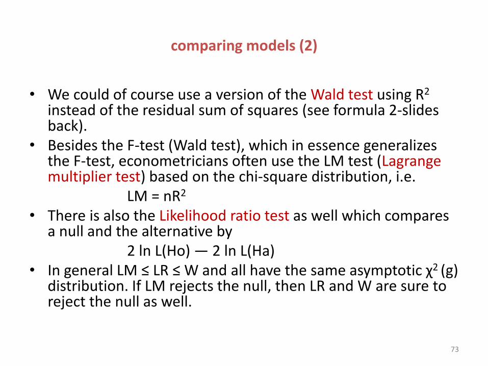
comparing models (2)

• We could of course use a version of the Wald test using R2 instead of the residual sum of squares (see formula 2-slides back).

• Besides the F-test (Wald test), which in essence generalizes the F-test, econometricians often use the LM test (Lagrange multiplier test) based on the chi-square distribution, i.e.

LM = nR2 • There is also the Likelihood ratio test as well which compares

a null and the alternative by 2 ln L(Ho) — 2 ln L(Ha) • In general LM ≤ LR ≤ W and all have the same asymptotic χ2 (g)

distribution. If LM rejects the null, then LR and W are sure to reject the null as well.

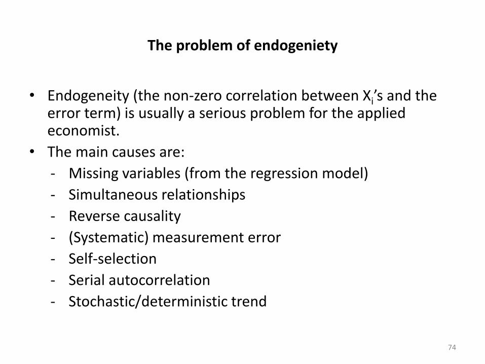
The problem of endogeniety

• Endogeneity (the non-zero correlation between Xi’s and the error term) is usually a serious problem for the applied economist.

• The main causes are:

- Missing variables (from the regression model)

- Simultaneous relationships

- Reverse causality

- (Systematic) measurement error

- Self-selection

- Serial autocorrelation

- Stochastic/deterministic trend

74

75

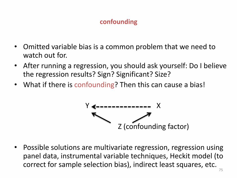
confounding

• Omitted variable bias is a common problem that we need to watch out for.

• After running a regression, you should ask yourself: Do I believe the regression results? Sign? Significant? Size?

• What if there is confounding? Then this can cause a bias!

Y X

Z (confounding factor)

• Possible solutions are multivariate regression, regression using panel data, instrumental variable techniques, Heckit model (to correct for sample selection bias), indirect least squares, etc.

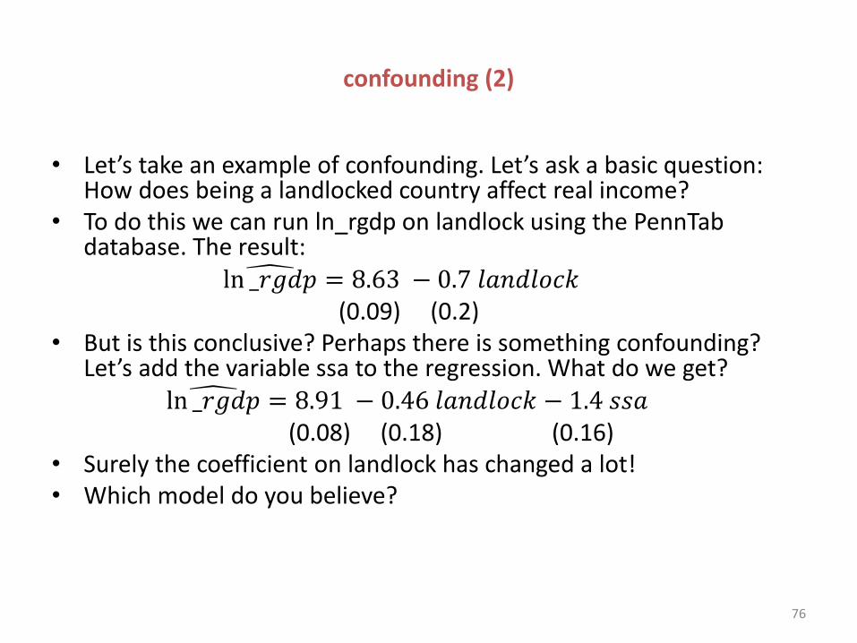
confounding (2)

• Let’s take an example of confounding. Let’s ask a basic question: How does being a landlocked country affect real income?

• To do this we can run ln_rgdp on landlock using the PennTab database. The result:

ln _𝑟𝑔𝑑𝑝 = 8.63 − 0.7 𝑙𝑎𝑛𝑑𝑙𝑜𝑐𝑘 (0.09) (0.2) • But is this conclusive? Perhaps there is something confounding?

Let’s add the variable ssa to the regression. What do we get?

ln _𝑟𝑔𝑑𝑝 = 8.91 − 0.46 𝑙𝑎𝑛𝑑𝑙𝑜𝑐𝑘 − 1.4 𝑠𝑠𝑎 (0.08) (0.18) (0.16) • Surely the coefficient on landlock has changed a lot! • Which model do you believe?

76

non-linear forms

• Economic relationships are not always linear. In the econometrics literature, non-linear relationships can be modelled using: – Quadratic transformations – Taking logs – Dummy regressions – Interaction variables

• Stata’s graphics allows for a quadratic fit with qfit which is used instead of lfit.

77

common errors you should avoid

• Confusing correlation/regression with causation

- Regression identifies association between variables; it cannot prove causality. Often the researcher will have to rely on theory to make causal arguments.

• Endogeneity: Cov(u, X’s) ≠ 0

- This causes estimates to be biased and is caused by among other things omitted variables, measurement error, reverse causality, sample selection, simultaneous relationship, and so on.

• Relying too much on R-squared

- Often a high R-squared does not mean out regression is any good (nor does a low R-squared mean that the regression is bad).

• Data-mining

- It is not acceptable to blindly run regressions (possibility of type-I and type-II errors). Theory should guide you.

78

79

what next?

• We have so far mainly looked at the classical regression method by OLS. The workshop will continue with more specific examples particularly related to gravity modelling.

• Stata has a rich library of commands for logistic/probit regression, panel-data analysis, time-series tools, as well as survey data and other multivariate statistical analyses.

• When dealing with other data forms, Stata requires that you declare the type of data, for example: . xtset n t // for panel data

. tsset t // for time-series

• For example, with survey data we invoke svyset, to declare survival-time data use stset, for mixed and multilevel data analysis we use xtmixed, and so on.

G O O D L U C K !

80

references (some of my favorites)

http://www.stata.com/support/faqs/ http://www.stata.com/links/resources1.html Statistics with Stata (Updated for Version 10) by Lawrence C. Hamilton An Introduction to Modern Econometrics Using Stata by Christopher F. Baum Microeconometrics Using Stata, Revised Edition by A. Colin Cameron and Pravin K. Trivedi • Hill, R. C., W. E. Griffiths, and G. C. Lim. 2011. Principles of Econometrics. 4th

ed. Hoboken, NJ: Wiley. • Adkins, L. C., and R. C. Hill. 2011. Using Stata for Principles of Econometrics.

4th ed. Hoboken, NJ: Wiley. • Stock, J. H., and M. W. Watson. 2011. Introduction to Econometrics. 3rd. ed

Addison Wesley • Verbeek, M. 2012. A Guide to Modern Econometrics. 4th ed. Wiley & Sons. • Wooldridge, J. M. 2012. Introductory Econometrics: A Modern Approach. 5th

ed. Cincinnati, OH: South-Western. • Wooldridge, J. M. 2010. Econometric Analysis of Cross Section and Panel Data.

Cambridge, MA: MIT Press. • Angrist, J. D., and J.-S. Pischke. 2009. Mostly Harmless Econometrics: An

Empiricist’s Companion. Princeton, NJ: Princeton University Press.