Welcome message from author
This document is posted to help you gain knowledge. Please leave a comment to let me know what you think about it! Share it to your friends and learn new things together.
Transcript
8/21/2019 Introduction to Lie Groups and Lie Algebras
http://slidepdf.com/reader/full/introduction-to-lie-groups-and-lie-algebras 1/236
8/21/2019 Introduction to Lie Groups and Lie Algebras
http://slidepdf.com/reader/full/introduction-to-lie-groups-and-lie-algebras 2/236
C A M B R I D G E S T U D I E S I N A D V A N C E D M A T H E M A T I C S
All the titles listed below can be obtained from good booksellers or from CambridgeUniversity Press. For a complete series listing visit: http://www.cambridge.org/series/ sSeries.asp?code=CSAM
Already published 60 M. P. Brodmann & R. Y. Sharp Local cohomology
61 J. D. Dixon et al. Analytic pro-p groups
62 R. Stanley Enumerative combinatorics II
63 R. M. Dudley Uniform central limit theorems
64 J. Jost & X. Li-Jost Calculus of variations
65 A. J. Berrick & M. E. Keating An introduction to rings and modules
66 S. Morosawa Holomorphic dynamics
67 A. J. Berrick & M. E. Keating Categories and modules with K-theory in view68 K. Sato Levy processes and infinitely divisible distributions
69 H. Hida Modular forms and Galois cohomology
70 R. Iorio & V. Iorio Fourier analysis and partial differential equations
71 R. Blei Analysis in integer and fractional dimensions
72 F. Borceaux & G. Janelidze Galois theories
73 B. Bollobás Random graphs
74 R. M. Dudley Real analysis and probability
75 T. Sheil-Small Complex polynomials
76 C. Voisin Hodge theory and complex algebraic geometry, I
77 C. Voisin Hodge theory and complex algebraic geometry, II
78 V. Paulsen Completely bounded maps and operator algebras
79 F. Gesztesy & H. Holden Soliton Equations and Their Algebro-Geometric Solutions, I 81 S. Mukai An Introduction to Invariants and Moduli
82 G. Tourlakis Lectures in Logic and Set Theory, I
83 G. Tourlakis Lectures in Logic and Set Theory, II
84 R. A. Bailey Association Schemes
85 J. Carison, S. Müller-Stach & C. Peters Period Mappings and Period Domains
86 J. J. Duistermaat & J. A. C. Kolk Multidimensional Real Analysis I
87 J. J. Duistermaat & J. A. C. Kolk Multidimensional Real Analysis II
89 M. Golumbic & A. Trenk Tolerance Graphs
90 L. Harper Global Methods for Combinatorial Isoperimetric Problems
91 I. Moerdijk & J. Mrcun Introduction to Foliations and Lie Groupoids
92 J. Kollar, K. E. Smith & A. Corti Rational and Nearly Rational Varieties
93 D. Applebaum Levy Processes and Stochastic Calculus
94 B. Conrad Modular Forms and the Ramanujan Conjecture95 M. Schechter An Introduction to Nonlinear Analysis
96 R. Carter Lie Algebras of Finite and Affine Type
97 H. L. Montgomery, R. C. Vaughan & M. Schechter Multiplicative Number Theory I
98 I. Chavel Riemannian Geometry
99 D. Goldfeld Automorphic Forms and L-Functions for the Group GL(n,R)
100 M. Marcus & J. Rosen Markov Processes. Gaussian Processes, and Local Times
101 P. Gille & T. Szamuely Central Simple Algebras and Galois Cohomology
102 J. Bertoin Random Fragmentation and Coagulation Processes
103 E. Frenkel Langlands Correspondence for Loop Groups
104 A. Ambrosetti & A. Malchiodi Nonlinear Analysis and Semilinear Elliptic Problems
105 T. Tao & V. H. Vu Additive Combinatorics
106 E. B. Davies Linear Operators and their Spectra107 K. Kodaira Complex Analysis
108 T. Ceccherini-Silberstein, F. Scarabotti & F. Tolli Harmonic Analysis on Finite Groups
8/21/2019 Introduction to Lie Groups and Lie Algebras
http://slidepdf.com/reader/full/introduction-to-lie-groups-and-lie-algebras 3/236
An Introduction to Lie Groups
and Lie Algebras
ALEXANDER KIRILLOV, Jr.
Department of Mathematics, SUNY at Stony Brook
8/21/2019 Introduction to Lie Groups and Lie Algebras
http://slidepdf.com/reader/full/introduction-to-lie-groups-and-lie-algebras 4/236
CAMBRIDGE UNIVERSITY PRESS
Cambridge, New York, Melbourne, Madrid, Cape Town, Singapore, São Paulo
Cambridge University PressThe Edinburgh Building, Cambridge CB2 8RU, UK
First published in print format
ISBN-13 978-0-521-88969-8
ISBN-13 978-0-511-42319-2
© A. Kirillov Jr. 2008
2008
Information on this title: www.cambridge.org/9780521889698
This publication is in copyright. Subject to statutory exception and to the provision ofrelevant collective licensing agreements, no reproduction of any part may take place
without the written permission of Cambridge University Press.
Cambridge University Press has no responsibility for the persistence or accuracy of urlsfor external or third-party internet websites referred to in this publication, and does notguarantee that any content on such websites is, or will remain, accurate or appropriate.
Published in the United States of America by Cambridge University Press, New York
www.cambridge.org
eBook (EBL)
hardback

8/21/2019 Introduction to Lie Groups and Lie Algebras
http://slidepdf.com/reader/full/introduction-to-lie-groups-and-lie-algebras 5/236
Dedicated to my teachers

8/21/2019 Introduction to Lie Groups and Lie Algebras
http://slidepdf.com/reader/full/introduction-to-lie-groups-and-lie-algebras 6/236
8/21/2019 Introduction to Lie Groups and Lie Algebras
http://slidepdf.com/reader/full/introduction-to-lie-groups-and-lie-algebras 7/236
Contents
Preface page xi
1 Introduction 1
2 Lie groups: basic definitions 4
2.1. Reminders from differential geometry 4
2.2. Lie groups, subgroups, and cosets 5
2.3. Lie subgroups and homomorphism theorem 10
2.4. Action of Lie groups on manifolds and
representations 10
2.5. Orbits and homogeneous spaces 12
2.6. Left, right, and adjoint action 14
2.7. Classical groups 16
2.8. Exercises 213 Lie groups and Lie algebras 25
3.1. Exponential map 25
3.2. The commutator 28
3.3. Jacobi identity and the definition of a Lie algebra 30
3.4. Subalgebras, ideals, and center 32
3.5. Lie algebra of vector fields 33
3.6. Stabilizers and the center 36
3.7. Campbell–Hausdorff formula 38
3 8 Fundamental theorems of Lie theory 40
8/21/2019 Introduction to Lie Groups and Lie Algebras
http://slidepdf.com/reader/full/introduction-to-lie-groups-and-lie-algebras 8/236
viii Contents
4 Representations of Lie groups and Lie algebras 52
4.1. Basic definitions 52
4.2. Operations on representations 54
4.3. Irreducible representations 57
4.4. Intertwining operators and Schur’s lemma 59
4.5. Complete reducibility of unitary representations:
representations of finite groups 61
4.6. Haar measure on compact Lie groups 62
4.7. Orthogonality of characters and Peter–Weyl theorem 65
4.8. Representations of sl(2,C
) 704.9. Spherical Laplace operator and the hydrogen atom 75
4.10. Exercises 80
5 Structure theory of Lie algebras 84
5.1. Universal enveloping algebra 84
5.2. Poincare–Birkhoff–Witt theorem 87
5.3. Ideals and commutant 90
5.4. Solvable and nilpotent Lie algebras 915.5. Lie’s and Engel’s theorems 94
5.6. The radical. Semisimple and reductive algebras 96
5.7. Invariant bilinear forms and semisimplicity of classical Lie
algebras 99
5.8. Killing form and Cartan’s criterion 101
5.9. Jordan decomposition 104
5.10. Exercises 106
6 Complex semisimple Lie algebras 108
6.1. Properties of semisimple Lie algebras 108
6.2. Relation with compact groups 110
6.3. Complete reducibility of representations 112
6.4. Semisimple elements and toral subalgebras 116
6.5. Cartan subalgebra 119
6.6. Root decomposition and root systems 120
6.7. Regular elements and conjugacy of Cartansubalgebras 126

8/21/2019 Introduction to Lie Groups and Lie Algebras
http://slidepdf.com/reader/full/introduction-to-lie-groups-and-lie-algebras 9/236
Contents ix
7.4. Positive roots and simple roots 137
7.5. Weight and root lattices 140
7.6. Weyl chambers 142
7.7. Simple reflections 146
7.8. Dynkin diagrams and classification of root systems 149
7.9. Serre relations and classification of semisimple
Lie algebras 154
7.10. Proof of the classification theorem in
simply-laced case 157
7.11. Exercises 160
8 Representations of semisimple Lie algebras 163
8.1. Weight decomposition and characters 163
8.2. Highest weight representations and Verma modules 167
8.3. Classification of irreducible finite-dimensional
representations 171
8.4. Bernstein–Gelfand–Gelfand resolution 174
8.5. Weyl character formula 177
8.6. Multiplicities 182
8.7. Representations of sl(n,C) 183
8.8. Harish–Chandra isomorphism 187
8.9. Proof of Theorem 8.25 192
8.10. Exercises 194
Overview of the literature 197
Basic textbooks 197
Monographs 198
Further reading 198
Appendix A Root systems and simple Lie algebras 202
A.1. An = sl(n + 1,C), n ≥ 1 202
A.2. Bn = so(2n + 1,C), n ≥ 1 204
A.3. C n = sp(n,C), n ≥ 1 206
A.4. Dn
= so(2n,C), n
≥ 2 207
Appendix B Sample syllabus 210

8/21/2019 Introduction to Lie Groups and Lie Algebras
http://slidepdf.com/reader/full/introduction-to-lie-groups-and-lie-algebras 10/236
8/21/2019 Introduction to Lie Groups and Lie Algebras
http://slidepdf.com/reader/full/introduction-to-lie-groups-and-lie-algebras 11/236
Preface
This book is an introduction to the theory of Lie groups and Lie algebras, with
emphasis on the theory of semisimple Lie algebras. It can serve as a basis for
a two-semester graduate course or – omitting some material – as a basis for
a rather intensive one-semester course. The book includes a large number of
exercises.
The material covered in the book ranges from basic definitions of Lie groupsto the theory of root systems and highest weight representations of semisim-
ple Lie algebras; however, to keep book size small, the structure theory of
semisimple and compact Lie groups is not covered.
Exposition follows the style of famous Serre’s textbook on Lie algebras
[47]: we tried to make the book more readable by stressing ideas of the proofs
rather than technical details. In many cases, details of the proofs are given
in exercises (always providing sufficient hints so that good students should
have no difficulty completing the proof). In some cases, technical proofs are
omitted altogether; for example, we do not give proofs of Engel’s or Poincare–
Birkhoff–Witt theorems, instead providing an outline of the proof. Of course,
in such cases we give references to books containing full proofs.
It is assumed that the reader is familiar with basics of topology and dif-
ferential geometry (manifolds, vector fields, differential forms, fundamental
groups, covering spaces) and basic algebra (rings, modules). Some parts of the
book require knowledge of basic homological algebra (short and long exactsequences, Ext spaces).
E f hi b k il bl h b k b

8/21/2019 Introduction to Lie Groups and Lie Algebras
http://slidepdf.com/reader/full/introduction-to-lie-groups-and-lie-algebras 12/236
8/21/2019 Introduction to Lie Groups and Lie Algebras
http://slidepdf.com/reader/full/introduction-to-lie-groups-and-lie-algebras 13/236
1
Introduction
In any algebra textbook, the study of group theory is usually mostly concerned
with the theory of finite, or at least finitely generated, groups. This is understand-
able: such groups are much easier to describe. However, most groups which
appear as groups of symmetries of various geometric objects are not finite: for
example, the group SO(3,R) of all rotations of three-dimensional space is not
finite and is not even finitely generated. Thus, much of material learned in basicalgebra course does not apply here; for example, it is not clear whether, say, the
set of all morphisms between such groups can be explicitly described.
The theory of Lie groups answers these questions by replacing the notion of a
finitely generated group by that of a Lie group – a group which at the same time
is a finite-dimensional manifold. It turns out that in many ways such groups
can be described and studied as easily as finitely generated groups – or even
easier. The key role is played by the notion of a Lie algebra, the tangent space
to G at identity. It turns out that the group operation on G defines a certain
bilinear skew-symmetric operation on g = T 1G; axiomatizing the properties
of this operation gives a definition of a Lie algebra.
The fundamental result of the theory of Lie groups is that many properties
of Lie groups are completely determined by the properties of corresponding
Lie algebras. For example, the set of morphisms between two (connected and
simply connected) Lie groups is the same as the set of morphisms between the
corresponding Lie algebras; thus, describing them is essentially reduced to alinear algebra problem.
Si il l Li l b l id k h d f h f Li
8/21/2019 Introduction to Lie Groups and Lie Algebras
http://slidepdf.com/reader/full/introduction-to-lie-groups-and-lie-algebras 14/236
2 Introduction
(including the author of this book) to be one of the most beautiful achievements
in all of mathematics. We will cover it in Chapter 7.
To conclude this introduction, we will give a simple example which shows
how Lie groups naturally appear as groups of symmetries of various objects –
and how one can use the theory of Lie groups and Lie algebras to make use of
these symmetries.
Let S 2 ⊂ R3 be the unit sphere. Define the Laplace operator sph :
C ∞(S 2) → C ∞(S 2) by sph f = (˜ f )|S 2 , where ˜ f is the result of extending
f to R3 − {0} (constant along each ray), and is the usual Laplace operator
in R3. It is easy to see that sph
is a second-order differential operator on the
sphere; one can write explicit formulas for it in the spherical coordinates, but
they are not particularly nice.
For many applications, it is important to know the eigenvalues and eigen-
functions of sph. In particular, this problem arises in quantum mechanics:
the eigenvalues are related to the energy levels of a hydrogen atom in quan-
tum mechanical description. Unfortunately, trying to find the eigenfunctions by
brute force gives a second-order differential equation which is very difficult to
solve.However, it is easy to notice that this problem has some symmetry – namely,
the group SO(3,R) acting on the sphere by rotations. How can one use this
symmetry?
If we had just one symmetry, given by some rotation R : S 2 → S 2, we could
consider its action on the space of complex-valued functions C ∞(S 2,C). If we
could diagonalize this operator, this would help us study sph: it is a general
result of linear algebra that if A, B are two commuting operators, and A is
diagonalizable, then B must preserve eigenspaces for A. Applying this to pair
R, sph, we get that sph preserves eigenspaces for R, so we can diagonalize
sph independently in each of the eigenspaces.
However, this will not solve the problem: for each individual rotation R, the
eigenspaces will still be too large (in fact, infinite-dimensional), so diagonaliz-
ing sph in each of them is not very easy either. This is not surprising: after all,
we only used one of many symmetries. Can we use all of rotations R ∈ SO(3,R)
simultaneously?This, however, presents two problems.
8/21/2019 Introduction to Lie Groups and Lie Algebras
http://slidepdf.com/reader/full/introduction-to-lie-groups-and-lie-algebras 15/236
Introduction 3
The goal of the theory of Lie groups is to give tools to deal with these (and
similar) problems. In short, the answer to the first problem is that SO(3,R) is in
a certain sense finitely generated – namely, it is generated by three generators,
“infinitesimal rotations” around x , y, z axes (see details in Example 3.10).
The answer to the second problem is that instead of decomposing the
C ∞(S 2,C) into a direct sum of common eigenspaces for operators R ∈SO(3,R), we need to decompose it into “irreducible representations” of
SO(3,R). In order to do this, we need to develop the theory of representa-
tions of SO(3,R). We will do this and complete the analysis of this example in
Section 4.8.
8/21/2019 Introduction to Lie Groups and Lie Algebras
http://slidepdf.com/reader/full/introduction-to-lie-groups-and-lie-algebras 16/236
2
Lie groups: basic definitions
2.1. Reminders from differential geometry
This book assumes that the reader is familiar with basic notions of differential
geometry, as covered for example, in [49]. For reader’s convenience, in this
section we briefly remind some definitions and fix notation.
Unless otherwise specified, all manifolds considered in this book will beC ∞ real manifolds; the word “smooth” will mean C ∞. All manifolds we will
consider will have at most countably many connected components.
For a manifold M and a point m ∈ M , we denote by T m M the tangent
space to M at point m, and by TM the tangent bundle to M . The space of
vector fields on M (i.e., global sections of TM ) is denoted by Vect( M ). For a
morphism f : X → Y and a point x ∈ X , we denote by f ∗ : T x X → T f ( x )Y the
corresponding map of tangent spaces.
Recall that a morphism f : X → Y is called an immersion if rank f ∗ = dim X for every point x ∈ X ; in this case, one can choose local coordinates in a
neighborhood of x ∈ X and in a neighborhood of f ( x ) ∈ Y such that f is given
by f ( x 1, . . . x n) = ( x 1, . . . , x n, 0, . . . 0).
An immersed submanifold in a manifold M isasubset N ⊂ M with a structure
of a manifold (not necessarily the one inherited from M !) such that inclusion
map i : N → M is an immersion. Note that the manifold structure on N is part
of the data: in general, it is not unique. However, it is usually suppressed in the
notation. Note also that for any point p ∈ N , the tangent space to N is naturally
a subspace of tangent space to M : T N ⊂ T M
8/21/2019 Introduction to Lie Groups and Lie Algebras
http://slidepdf.com/reader/full/introduction-to-lie-groups-and-lie-algebras 17/236
2.2. Lie groups, subgroups, and cosets 5
All of the notions above have complex analogs, in which real manifolds
are replaced by complex analytic manifolds and smooth maps by holomorphic
maps. We refer the reader to [49] for details.
2.2. Lie groups, subgroups, and cosets
Definition 2.1. A(real)Liegroupisaset G with two structures: G isagroupand
G is a manifold. These structures agree in the following sense: multiplication
map G
×G
→ G and inversion map G
→ G are smooth maps.
A morphism of Lie groups is a smooth map which also preserves the group
operation: f (gh) = f (g) f (h), f (1) = 1. We will use the standard notation Im f ,
Ker f for image and kernel of a morphism.
The word “real” is used to distinguish these Lie groups from complex Lie
groups defined below. However, it is frequently omitted: unless one wants to
stress the difference with complex case, it is common to refer to real Lie groups
as simply Lie groups.
Remark 2.2. One can also consider other classes of manifolds: C 1, C 2, ana-
lytic. It turns out that all of them are equivalent: every C 0 Lie group has a unique
analytic structure. This is a highly non-trivial result (it was one of Hilbert’s 20
problems), and we are not going to prove it (the proof can be found in the
book [39]). Proof of a weaker result, that C 2 implies analyticity, is much easier
and can be found in [10, Section 1.6]. In this book, “smooth” will be always
understood as C ∞.
In a similar way, one defines complex Lie groups.
Definition 2.3. A complex Lie group is a set G with two structures: G is a group
and G is a complex analytic manifold. These structures agree in the following
sense: multiplication map G × G → G and inversion map G → G are analytic
maps.
A morphism of complex Lie groups is an analytic map which also preserves
the group operation: f (gh)
= f (g) f (h), f (1)
= 1.
Remark 2.4. Throughout this book, we try to treat both real and complex
i l l Th h i hi b k l b h l d
8/21/2019 Introduction to Lie Groups and Lie Algebras
http://slidepdf.com/reader/full/introduction-to-lie-groups-and-lie-algebras 18/236
6 Lie groups: basic definitions
vector spaces, all morphisms between manifolds will be assumed holomor-
phic, etc.
Example 2.5. The following are examples of Lie groups:
(1) Rn, with the group operation given by addition
(2) R∗ = R \ {0}, ×R+ = { x ∈ R| x > 0}, ×
(3) S 1 = { z ∈ C : | z| = 1}, ×(4) GL(n,R)
⊂ Rn2
. Many of the groups we will consider will be subgroups
of GL(n,R) or GL(n,C).(5) SU(2) = { A ∈ GL(2,C) | A ¯ At = 1, det A = 1}. Indeed, one can easily see
that
SU(2) =
α β
−β α
: α , β ∈ C, |α|2 + |β|2 = 1
.
Writing α
= x 1
+ i x 2, β
= x 3
+ i x 4, x i
∈ R, we see that SU(2) is
diffeomorphic to S 3 = { x 21 + · · · + x 24 = 1} ⊂ R4.
(6) In fact, all usual groups of linear algebra, such as GL(n,R), SL(n,R),
O(n,R), U(n), SO(n,R), SU(n), Sp(n,R) are (real or complex) Lie groups.
This will be proved later (see Section 2.7).
Note that the definition of a Lie group does not require that G be connected.
Thus, any finite group is a 0-dimensional Lie group. Since the theory of finite
groups is complicated enough, it makes sense to separate the finite (or, more
generally, discrete) part. It can be done as follows.
Theorem 2.6. Let G be a real or complex Lie group. Denote by G0 the connected
component of identity. Then G0 is a normal subgroup of G and is a Lie group
itself (real or complex, respectively). The quotient group G/G0 is discrete.
Proof. We need to show that G0 is closed under the operations of multiplica-
tion and inversion. Since the image of a connected topological space under acontinuous map is connected, the inversion map i must take G0 to one com-
f G h hi h i i(1) 1 l G0 I i il

8/21/2019 Introduction to Lie Groups and Lie Algebras
http://slidepdf.com/reader/full/introduction-to-lie-groups-and-lie-algebras 19/236
2.2. Lie groups, subgroups, and cosets 7
This theorem mostly reduces the study of arbitrary Lie groups to the study of
finite groups and connected Lie groups. In fact, one can go further and reduce
the study of connected Lie groups to connected simply-connected Lie groups.
Theorem 2.7. If G is a connected Lie group (real or complex ) , then its universal
cover G has a canonical structure of a Lie group (real or complex, respec-
tively) such that the covering map p : G → G is a morphism of Lie groups
whose kernel is isomorphic to the fundamental group of G: Ker p = π1(G)
as a group. Moreover, in this case Ker p is a discrete central subgroup
in
˜G.
Proof. The proof follows from the following general result of topology: if
M , N are connected manifolds (or, more generally, nice enough topological
spaces), then any continuous map f : M → N can be lifted to a map of universal
covers ˜ f : ˜ M → ˜ N . Moreover, if we choose m ∈ M , n ∈ N such that f (m) = n
and choose liftings m ∈ ˜ M , n ∈ ˜ N such that p(m) = m, p(n) = n, then there is
a unique lifting ˜ f of f such that ˜ f (m) = n.
Now let us choose some element 1 ∈ G such that p(1) = 1 ∈ G. Then, bythe above theorem, there is a unique map ı : G → G which lifts the inversion
map i : G → G and satisfies ı(1) = 1. In a similar way one constructs the
multiplication map G × G → G. Details are left to the reader.
Finally, the fact that Ker p is central follows from results of Exercise 2.2.
Definition 2.8. A closed Lie subgroup H of a (real or complex) Lie group G is
a subgroup which is also a submanifold (for complex Lie groups, it is must be
a complex submanifold).
Note that the definition does not require that H be a closed subset in G; thus,
the word “closed” requires some justification which is given by the following
result.
Theorem 2.9.
(1) Any closed Lie subgroup is closed in G.(2) Any closed subgroup of a Lie group is a closed real Lie subgroup.
8/21/2019 Introduction to Lie Groups and Lie Algebras
http://slidepdf.com/reader/full/introduction-to-lie-groups-and-lie-algebras 20/236
8 Lie groups: basic definitions
Corollary 2.10.
(1) If G is a connected Lie group (real or complex ) and U is a neighborhood of 1 , then U generates G.
(2) Let f : G1 → G2 be a morphism of Lie groups (real or complex ) , with
G2 connected, such that f ∗ : T 1G1 → T 1G2 is surjective. Then f is
surjective.
Proof. (1) Let H be the subgroup generated by U . Then H is open in G: for
any element h ∈ H , the set h · U is a neighborhood of h in G. Since
it is an open subset of a manifold, it is a submanifold, so H is a
closed Lie subgroup. Therefore, by Theorem 2.9 it is closed, and is
nonempty, so H = G.
(2) Given the assumption, the inverse function theorem says that f is
surjective onto some neighborhood U of 1 ∈ G2. Since an image
of a group morphism is a subgroup, and U generates G2, f is
surjective.
As in the theory of discrete groups, given a closed Lie subgroup H
⊂ G,
we can define the notion of cosets and define the coset space G/ H as the set
of equivalence classes. The following theorem shows that the coset space is
actually a manifold.
Theorem 2.11.
(1) Let G be a (real or complex ) Lie group of dimension n and H ⊂ G a closed
Lie subgroup of dimension k. Then the coset space G/ H has a natural
structure of a manifold of dimension n − k such that the canonical map p : G → G/ H is a fiber bundle, with fiber diffeomorphic to H . The tangent
space at 1 = p(1) is given by T 1(G/ H ) = T 1G/T 1 H .
(2) If H is a normal closed Lie subgroup then G/ H has a canonical structure
of a Lie group (real or complex, respectively).
Proof. Denote by p : G → G/ H the canonical map. Let g ∈ G and g = p(g) ∈G/ H . Then the set g · H is a submanifold in G as it is an image of H under
diffeomorphism x → gx . Choose a submanifold M ⊂ G such that g ∈ M and M is transversal to the manifold gH , i.e. T g G = (T g (gH )) ⊕ T g M (this
i li h di M di G di H ) L U M b ffi i l ll
8/21/2019 Introduction to Lie Groups and Lie Algebras
http://slidepdf.com/reader/full/introduction-to-lie-groups-and-lie-algebras 21/236
2.2. Lie groups, subgroups, and cosets 9
M
U
g
G / H g
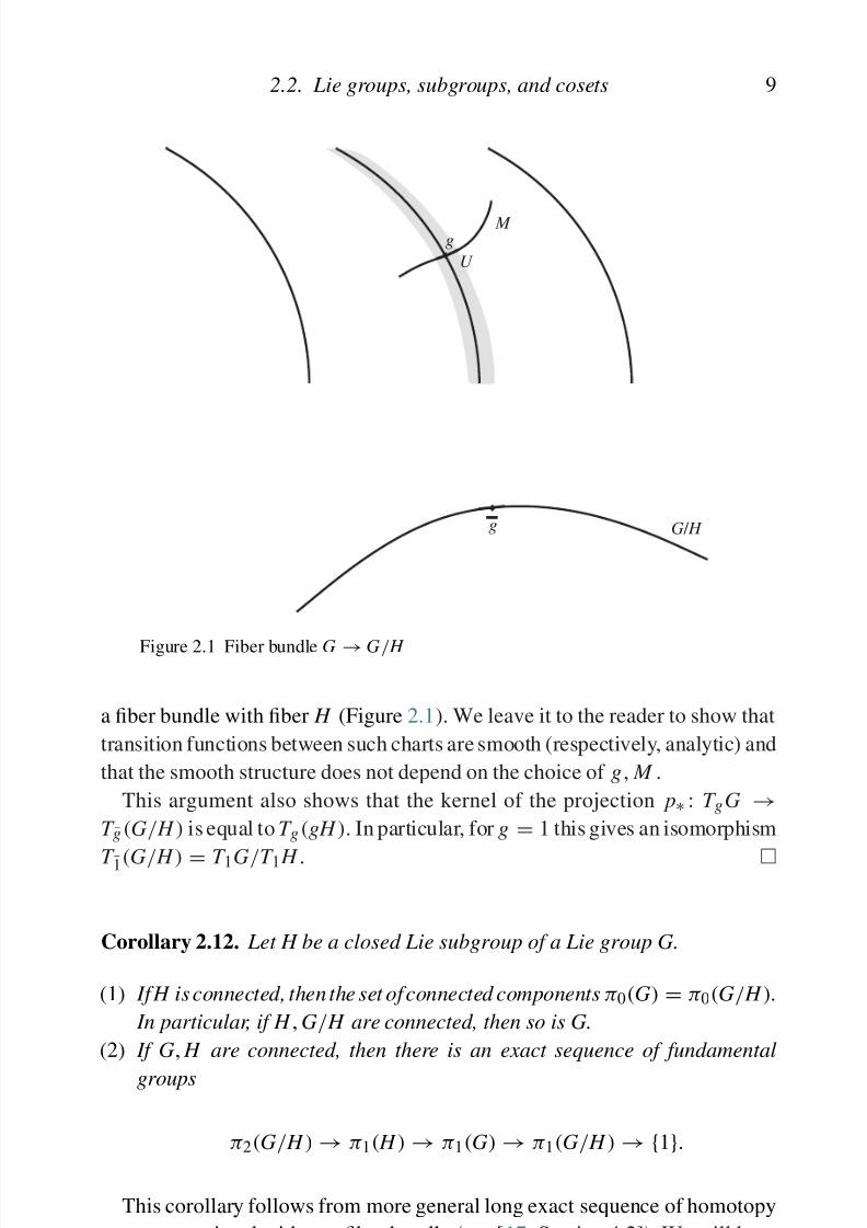
Figure 2.1 Fiber bundle G → G/ H
a fiber bundle with fiber H (Figure 2.1). We leave it to the reader to show that
transition functions between such charts are smooth (respectively, analytic) and
that the smooth structure does not depend on the choice of g , M .
This argument also shows that the kernel of the projection p∗ : T g G →T g (G/ H ) is equal to T g (gH ). In particular, for g = 1 this gives an isomorphism
T 1(G/ H ) = T 1G/T 1 H .
Corollary 2.12. Let H be a closed Lie subgroup of a Lie group G.
(1) If H is connected, then the set of connected components π0(G) = π0(G/ H ).
In particular, if H , G/ H are connected, then so is G.
(2) If G, H are connected, then there is an exact sequence of fundamental
groups
8/21/2019 Introduction to Lie Groups and Lie Algebras
http://slidepdf.com/reader/full/introduction-to-lie-groups-and-lie-algebras 22/236
10 Lie groups: basic definitions
2.3. Lie subgroups and homomorphism theorem
For many purposes, the notion of closed Lie subgroup introduced above is toorestrictive. For example, the image of a morphism may not be a closed Lie
subgroup, as the following example shows.
Example 2.13. Let G1 = R, G2 = T 2 = R2/Z2. Define the map f : G1 → G2
by f (t ) = (t mod Z, αt mod Z), where α is some fixed irrational number.
Then it is well-known that the image of this map is everywhere dense in T 2 (it
is sometimes called the irrational winding on the torus).
Thus, it is useful to introduce a more general notion of a subgroup. Recallthe definition of immersed submanifold (see Section 2.1).
Definition 2.14. An Lie subgroup in a (real or complex) Lie group H ⊂ G is
an immersed submanifold which is also a subgroup.
It is easy to see that in such a situation H is itself a Lie group (real or complex,
respectively) and the inclusion map i : H → G is a morphism of Lie groups.
Clearly, every closed Lie subgroup is a Lie subgroup, but the converse is
not true: the image of the map R → T 2 constructed in Example 2.13 is a Lie
subgroup which is not closed. It can be shown if a Lie subgroup is closed in
G, then it is automatically a closed Lie subgroup in the sense of Definition 2.8,
which justifies the name. We do not give a proof of this statement as we are not
going to use it.
With this new notion of a subgroup we can formulate an analog of the standard
homomorphism theorems.
Theorem 2.15. Let f : G1 → G2 be a morphism of (real or complex ) Lie
groups. Then H = Ker f is a normal closed Lie subgroup in G1 , and f gives
rise to an injective morphism G1/ H → G2 , which is an immersion; thus, Im f
is a Lie subgroup in G2. If Im f is an (embedded ) submanifold, then it is a closed
Lie subgroup in G2 and f gives an isomorphism of Lie groups G1/ H Im f .
The easiest way to prove this theorem is by using the theory of Lie algebras
which we will develop in the next chapter; thus, we postpone the proof until
the next chapter (see Corollary 3.30).

8/21/2019 Introduction to Lie Groups and Lie Algebras
http://slidepdf.com/reader/full/introduction-to-lie-groups-and-lie-algebras 23/236
2.4. Action of Lie groups on manifolds and representations 11
Definition 2.16. An action of a real Lie group G on a manifold M is an
assignment to each g
∈ G a diffeomorphism ρ(g)
∈ Diff M such that
ρ(1) = id, ρ(gh) = ρ(g)ρ(h) and such that the map
G × M → M : (g, m) → ρ(g).m
is a smooth map.
A holomorphic action of a complex Lie group G on a complex manifold M
is an assignment to each g ∈ G an invertible holomorphic map ρ (g) ∈ Diff M
such that ρ (1)
= id, ρ(gh)
= ρ(g)ρ(h) and such that the map
G × M → M : (g, m) → ρ(g).m
is holomorphic.
Example 2.17.
(1) The group GL(n,R) (and thus, any its closed Lie subgroup) acts on Rn.
(2) The group O(n,R) acts on the sphere S n−1
⊂Rn. The group U(n) acts on
the sphere S 2n−1 ⊂ Cn.
Closely related with the notion of a group action on a manifold is the notion
of a representation.
Definition 2.18. A representation of a (real or complex) Lie group G is a vector
space V (complex if G is complex, and either real or complex if G is real)
together with a group morphism ρ : G → End(V ). If V is finite-dimensional,
we require that ρ be smooth (respectively, analytic), so it is a morphism of Lie
groups. A morphism between two representations V , W of the same group G
is a linear map f : V → W which commutes with the group action: f ρV (g) =ρW (g) f .
In other words, we assign to every g ∈ G a linear map ρ(g) : V → V so that
ρ(g)ρ(h) = ρ(gh).
We will frequently use the shorter notation g .m, g.v instead of ρ (g).m in the
cases when there is no ambiguity about the representation being used.
Remark 2.19. Note that we frequently consider representations on a complex
f l i
8/21/2019 Introduction to Lie Groups and Lie Algebras
http://slidepdf.com/reader/full/introduction-to-lie-groups-and-lie-algebras 24/236
12 Lie groups: basic definitions
complex case) defined by
(ρ(g) f )(m) = f (g−1.m) (2.1)
(note that we need g−1 rather than g to satisfy ρ (g)ρ(h) = ρ(gh)).
(2) Representation of G on the (infinite-dimensional) space of vector fields
Vect( M ) defined by
(ρ(g).v)(m) = g∗(v(g−1.m)). (2.2)
In a similar way, we define the action of G on the spaces of differential
forms and other types of tensor fields on M .
(3) Assume that m ∈ M is a fixed point: g.m = m for any g ∈ G. Then we
have a canonical action of G on the tangent space T m M given by ρ(g) =g∗ : T m M → T m M , and similarly for the spaces T ∗m M ,
k T ∗m M .
2.5. Orbits and homogeneous spaces
Let G be a Lie group acting on a manifold M (respectively, a complex Lie group
acting on a complex manifold M ). Then for every point m ∈ M we define its
orbit by Om = Gm = {g.m | g ∈ G} and stabilizer by
Gm = {g ∈ G | g.m = m}. (2.3)
Theorem 2.20. Let M be a manifold with an action of a Lie group G (respec-tively, a complex manifold with an action of complex Lie group G). Then for
any m ∈ M the stabilizer Gm is a closed Lie subgroup in G, and g → g.m is an
injective immersion G/Gm → M whose image coincides with the orbit Om.
Proof. The fact that the orbit is in bijection with G/Gm is obvious. For the proof
of the fact that Gm is a closed Lie subgroup, we could just refer to Theorem 2.9.
However, this would not help proving that G/Gm → M is an immersion. Both
of these statements are easiest proved using the technique of Lie algebras; thus,we postpone the proof until later (see Theorem 3.29).
8/21/2019 Introduction to Lie Groups and Lie Algebras
http://slidepdf.com/reader/full/introduction-to-lie-groups-and-lie-algebras 25/236
2.5. Orbits and homogeneous spaces 13
Definition 2.22. A G-homogeneous space is a manifold with a transitive action
of G.
As an immediate corollary of Corollary 2.21, we see that each homogeneous
space is diffeomorphic to a coset space G/ H . Combining it with Theorem 2.11,
we get the following result.
Corollary 2.23. Let M be a G-homogeneous space and choose m ∈ M . Then
the map G → M : g → gm is a fiber bundle over M with fiber Gm.
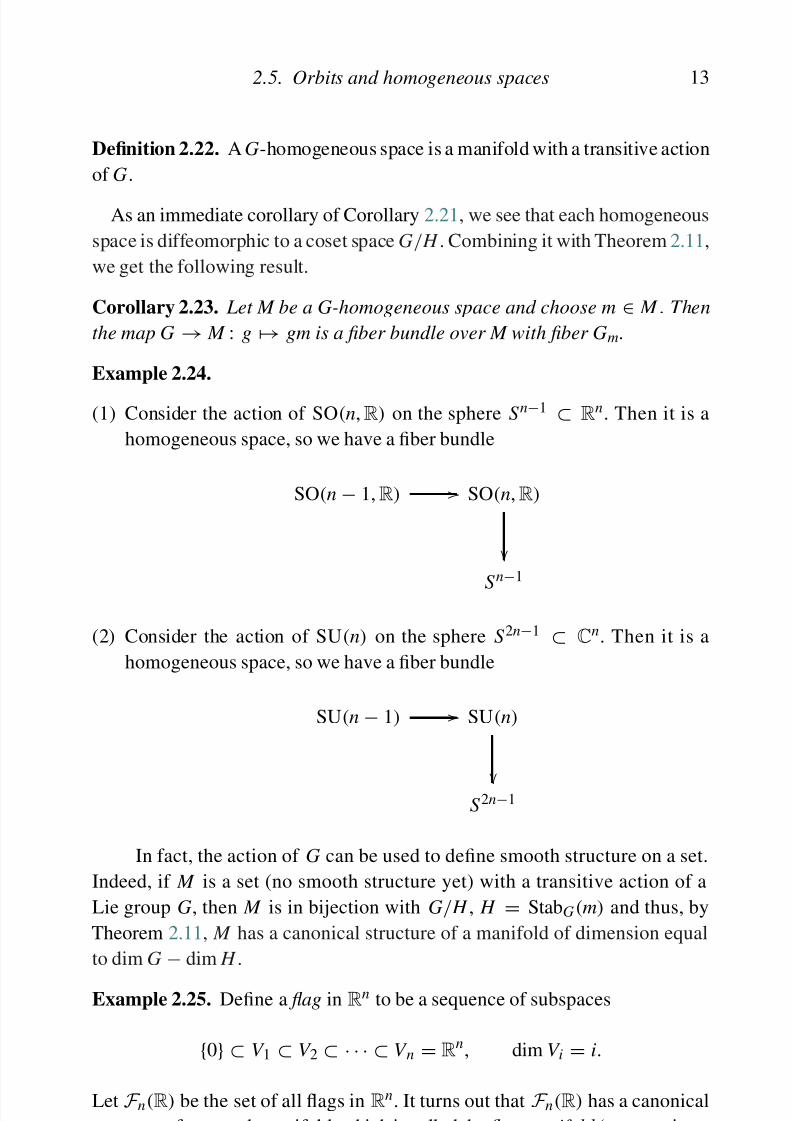
Example 2.24.
(1) Consider the action of SO(n,R) on the sphere S n−1 ⊂ Rn. Then it is a
homogeneous space, so we have a fiber bundle
SO(n − 1,R) SO(n,R)
S n
−1
(2) Consider the action of SU(n) on the sphere S 2n−1 ⊂ Cn. Then it is a
homogeneous space, so we have a fiber bundle
SU(n − 1) SU(n)
S 2n−1
In fact, the action of G can be used to define smooth structure on a set.
Indeed, if M is a set (no smooth structure yet) with a transitive action of a
Lie group G, then M is in bijection with G/ H , H = StabG(m) and thus, by
Theorem 2.11, M has a canonical structure of a manifold of dimension equal
to dim G
−dim H .
Example 2.25. Define a flag in Rn to be a sequence of subspaces
8/21/2019 Introduction to Lie Groups and Lie Algebras
http://slidepdf.com/reader/full/introduction-to-lie-groups-and-lie-algebras 26/236
14 Lie groups: basic definitions
action of the group GL(n,R) on F n(R). This action is transitive: by a change
of basis, any flag can be identified with the standard flag
V st = {0} ⊂ e1 ⊂ e1, e2 ⊂ · · · ⊂ e1, . . . , en−1 ⊂ Rn
,
where e1, . . . , ek stands for the subspace spanned by e1, . . . , ek . Thus, F n(R)
can be identified with the coset space GL(n,R)/ B(n,R), where B(n,R) =Stab V st is the group of all invertible upper-triangular matrices. Therefore, F n
is a manifold of dimension equal to n2 − (n(n + 1))/2 = n(n − 1)/2.
Finally, we should say a few words about taking the quotient by the action of
a group. In many cases when we have an action of a group G on a manifold M
one would like to consider the quotient space, i.e. the set of all G-orbits. This
set is commonly denoted by M /G. It has a canonical quotient space topology.
However, this space can be very singular, even if G is a Lie group; for example,
it can be non-Hausdorff. For example, for the group G = GL(n,C) acting on
the set of all n × n matrices by conjugation the set of orbits is described by
Jordan canonical form. However, it is well-known that by a small perturbation,
any matrix can be made diagonalizable. Thus, if X is a diagonalizable matrix
and Y is a non-diagonalizable matrix with the same eigenvalues as X , then any
neighborhood of the orbit of Y contains points from orbit of X .
There are several ways of dealing with this problem. One of them is to impose
additional requirements on the action, for example assuming that the action is
proper. In this case it can be shown that M /G is indeed a Hausdorff topological
space, and under some additional conditions, it is actually a manifold (see [10,
Section 2]). Another approach, usually called Geometric Invariant Theory, isbased on using the methods of algebraic geometry (see [40]). Both of these
methods go beyond the scope of this book.
2.6. Left, right, and adjoint action
Important examples of group action are the following actions of G on itself:
Left action: Lg : G → G is defined by Lg (h) = gh
8/21/2019 Introduction to Lie Groups and Lie Algebras
http://slidepdf.com/reader/full/introduction-to-lie-groups-and-lie-algebras 27/236
2.6. Left, right, and adjoint action 15
As mentioned in Section 2.4, each of these actions also defines the action of
G on the spaces of functions, vector fields, forms, etc. on G. For simplicity, for
a tangent vector v ∈ T mG , we will frequently write just g.v ∈ T gmG instead
of the technically more accurate but cumbersome notation ( Lg )∗v. Similarly,
we will write v.g for ( Rg−1 )∗v. This is justified by Exercise 2.6, where it is
shown that for matrix groups this notation agrees with the usual multiplication
of matrices.
Since the adjoint action preserves the identity element 1 ∈ G, it also defines
an action of G on the (finite-dimensional) space T 1G. Slightly abusing the
notation, we will denote this action also by
Ad g : T 1G → T 1G. (2.4)
Definition 2.26. A vector field v ∈ Vect(G) is left-invariant if g.v = v for
every g ∈ G, and right-invariant if v.g = v for every g ∈ G. A vector field is
called bi-invariant if it is both left- and right-invariant.
In a similar way one defines left- , right-, and bi-invariant differential formsand other tensors.
Theorem 2.27. The map v → v(1) (where 1 is the identity element of the group)
defines an isomorphism of the vector space of left-invariant vector fields on G
with the vector space T 1G, and similarly for right-invariant vector spaces.
Proof. It suffices to prove that every x ∈ T 1G can be uniquely extended to a
left-invariant vector field on G. Let us define the extension by v
(g) = g. x ∈T g G. Then one easily sees that the so-defined vector field is left-invariant, and
v(1) = x . This proves the existence of an extension; uniqueness is obvious.
Describing bi-invariant vector fields on G is more complicated: any x ∈ T 1G
can be uniquely extended to a left-invariant vector field and to a right-invariant
vector field, but these extensions may differ.
Theorem 2.28. The map v
→ v(1) defines an isomorphism of the vector space
of bi-invariant vector fields on G with the vector space of invariants of adjoint
action:
8/21/2019 Introduction to Lie Groups and Lie Algebras
http://slidepdf.com/reader/full/introduction-to-lie-groups-and-lie-algebras 28/236
16 Lie groups: basic definitions
2.7. Classical groups
In this section, we discuss the so-called classical groups, or various sub-groups of the general linear group which are frequently used in linear algebra.
Traditionally, the name “classical groups” is applied to the following groups:
• GL(n,K) (here and below, K is either R, which gives a real Lie group, or C,
which gives a complex Lie group)
• SL(n,K)
• O(n,K)
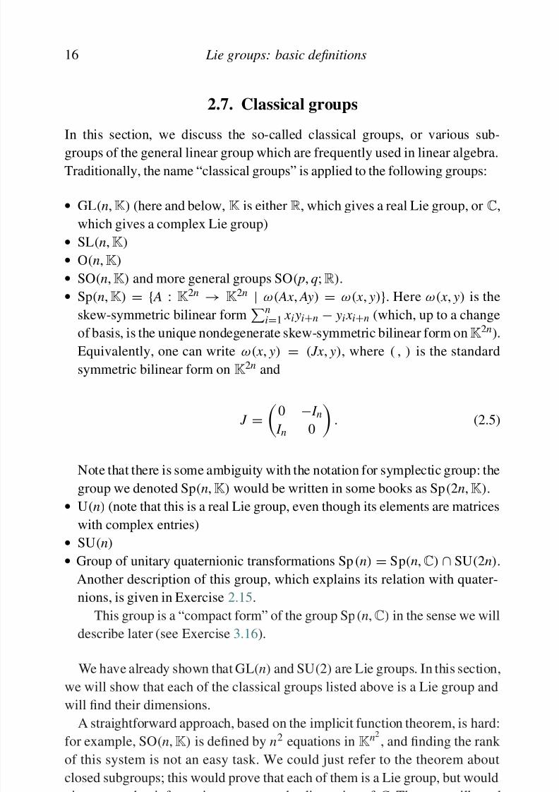
• SO(n,K) and more general groups SO( p, q;R).• Sp(n,K) = { A : K2n → K2n | ω( Ax , Ay) = ω( x , y)}. Here ω( x , y) is the
skew-symmetric bilinear formn
i=1 x i yi+n − yi x i+n (which, up to a change
of basis, is the unique nondegenerate skew-symmetric bilinear form onK2n).
Equivalently, one can write ω( x , y) = ( Jx , y), where ( , ) is the standard
symmetric bilinear form on K2n and
J = 0 − I n I n 0
. (2.5)
Note that there is some ambiguity with the notation for symplectic group: the
group we denoted Sp(n,K) would be written in some books as Sp(2n,K).
• U(n) (note that this is a real Lie group, even though its elements are matrices
with complex entries)
• SU(n)
• Group of unitary quaternionic transformations Sp(n) = Sp(n,C) ∩ SU(2n).
Another description of this group, which explains its relation with quater-
nions, is given in Exercise 2.15.
This group is a “compact form” of the group Sp(n,C) in the sense we will
describe later (see Exercise 3.16).
We have already shown that GL(n) and SU(2) are Lie groups. In this section,
we will show that each of the classical groups listed above is a Lie group andwill find their dimensions.
A i h f d h b d h i li i f i h i h d
8/21/2019 Introduction to Lie Groups and Lie Algebras
http://slidepdf.com/reader/full/introduction-to-lie-groups-and-lie-algebras 29/236
2.7. Classical groups 17
Our approach is based on the use of exponential map. Recall that for matrices,
the exponential map is defined by
exp( x ) =∞0
x k
k ! . (2.6)
It is well-known that this power series converges and defines an analytic map
gl(n,K) → gl(n,K), where gl(n,K) is the set of all n × n matrices. In a similar
way, we define the logarithmic map by
log(1 + x ) = ∞1
(−1)k +1 x k
k . (2.7)
So defined, log is an analytic map defined in a neighborhood of 1 ∈ gl(n,K).
The following theorem summarizes the properties of exponential and log-
arithmic maps. Most of the properties are the same as for numbers; however,
there are also some differences due to the fact that multiplication of matrices
is not commutative. All of the statements of this theorem apply equally in real
and complex cases.
Theorem 2.29.
(1) log(exp( x )) = x; exp(log( X )) = X whenever they are defined.
(2) exp( x ) = 1 + x + . . . This means exp(0) = 1 and d exp(0) = id .
(3) If xy = yx then exp( x + y) = exp( x ) exp( y). If XY = YX then log( XY ) =log( X ) + log(Y ) in some neighborhood of the identity. In particular, for
any x ∈ gl(n,K) , exp( x ) exp(− x ) = 1 , so exp x ∈ GL(n,K).(4) For fixed x ∈ gl(n,K) , consider the map K → GL(n,K) : t → exp(tx ).
Then exp((t + s) x ) = exp(tx ) exp(sx ). In other words, this map is a
morphism of Lie groups.
(5) The exponential map agrees with change of basis and transposition:
exp( AxA−1) = A exp( x ) A−1 , exp( x t ) = (exp( x ))t .
A full proof of this theorem will not be given here; instead, we just give a
sketch. The first two statements are just equalities of formal power series in onevariable; thus, it suffices to check that they hold for x ∈ R. Similarly, the third
i id i f f l i i i i bl i i
8/21/2019 Introduction to Lie Groups and Lie Algebras
http://slidepdf.com/reader/full/introduction-to-lie-groups-and-lie-algebras 30/236
18 Lie groups: basic definitions
How does it help us to study various matrix groups? The key idea is that the
logarithmic map identifies some neighborhood of the identity in GL(n,K) with
some neighborhood of 0 in the vector space gl(n,K). It turns out that it also
does the same for all of the classical groups.
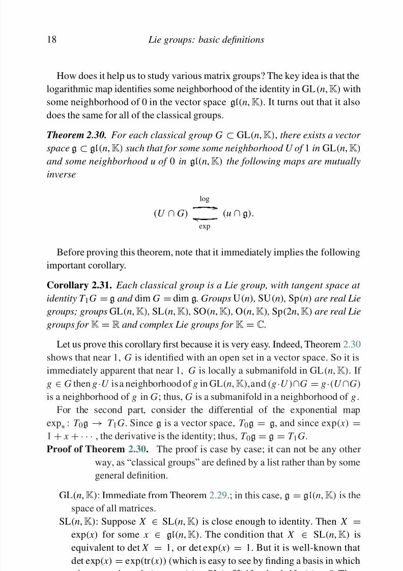
Theorem 2.30. For each classical group G ⊂ GL(n,K), there exists a vector
space g ⊂ gl(n,K) such that for some some neighborhood U of 1 in GL(n,K)
and some neighborhood u of 0 in gl(n,K) the following maps are mutually
inverse
(U ∩ G)log
exp
(u ∩ g).
Before proving this theorem, note that it immediately implies the following
important corollary.
Corollary 2.31. Each classical group is a Lie group, with tangent space at
identity T 1G = g and dim G = dim g. Groups U(n) , SU(n) , Sp(n) are real Liegroups; groups GL(n,K) , SL(n,K) , SO(n,K) , O(n,K) , Sp(2n,K) are real Lie
groups for K = R and complex Lie groups for K = C.
Let us prove this corollary first because it is very easy. Indeed, Theorem 2.30
shows that near 1, G is identified with an open set in a vector space. So it is
immediately apparent that near 1, G is locally a submanifold in GL(n,K). If
g ∈ G then g·U is a neighborhood of g in GL(n,K),and (g·U )∩G = g·(U ∩G)
is a neighborhood of g in G; thus, G is a submanifold in a neighborhood of g .For the second part, consider the differential of the exponential map
exp∗ : T 0g → T 1G. Since g is a vector space, T 0g = g, and since exp( x ) =1 + x + · · · , the derivative is the identity; thus, T 0g = g = T 1G.
Proof of Theorem 2.30. The proof is case by case; it can not be any other
way, as “classical groups” are defined by a list rather than by some
general definition.
GL(n,K
): Immediate from Theorem 2.29.; in this case, g = gl(n,K
) is thespace of all matrices.
SL( K) S X SL( K) i l h id i Th X

8/21/2019 Introduction to Lie Groups and Lie Algebras
http://slidepdf.com/reader/full/introduction-to-lie-groups-and-lie-algebras 31/236
2.7. Classical groups 19
O(n,K), SO(n,K): The group O(n,K) is defined by XX t = I . Then X , X t
commute. Writing X
= exp( x ), X t
= exp( x t ) (since the exponential
map agrees with transposition), we see that x , x t also commute, and thus
exp( x ) ∈ O(n,K) implies exp( x ) exp( x t ) = exp( x + x t ) = 1, so x + x t =0; conversely, if x + x t = 0, then x , x t commute, so we can reverse
the argument to get exp( x ) ∈ O(n,K). Thus, in this case the theorem
also holds, with g = { x | x + x t = 0} – the space of skew-symmetric
matrices.
What about SO(n,K)? In this case, we should add to the condition
XX t
= 1 (which gives x
+ x t
= 0) also the condition det X
= 1, which
gives tr( x ) = 0. However, this last condition is unnecessary, because
x + x t = 0 implies that all diagonal entries of x are zero. So both O(n,K)
and SO(n,K) correspond to the same space of matrices g = { x | x + x t =0}. This might seem confusing until one realizes that SO(n,K) is exactly
the connected component of identity in O(n,K); thus, a neighborhood of
1 in O(n,K) coincides with a neighborhood of 1 in SO(n,K).
U(n), SU(n): A similar argument shows that for x in a neighborhood of the
identity in gl(n,C), exp x ∈ U(n) ⇐⇒ x + x ∗ = 0 (where x ∗ = ¯ x t )
and exp x ∈ SU(n) ⇐⇒ x + x ∗ = 0,tr( x ) = 0. Note that in this case,
x + x ∗ does not imply that x has zeroes on the diagonal: it only implies
that the diagonal entries are purely imaginary. Thus, tr x = 0 does not
follow automatically from x + x ∗ = 0, so in this case the tangent spaces
for U(n), SU(n) are different.
Sp(n,K): A similar argument shows that exp( x ) ∈ Sp(n,K) ⇐⇒ x + J −1 x t J
= 0 where J is given by (2.5). Thus, in this case the theorem also
holds.
Sp(n): The same arguments as above show that exp( x ) ∈ Sp(n) ⇐⇒ x + J −1 x t J = 0, x + x ∗ = 0.
The vector space g = T 1G is called the Lie algebra of the corresponding
group G (this will be justified later, when we actually define an algebra operation
on it). Traditionally, the Lie algebra is denoted by lowercase letters using Fraktur
(Old German) fonts: for example, the Lie algebra of group SU(n) is denotedby su(n).
Th 2 30 i “l l” i f i b l i l Li i h
8/21/2019 Introduction to Lie Groups and Lie Algebras
http://slidepdf.com/reader/full/introduction-to-lie-groups-and-lie-algebras 32/236
20 Lie groups: basic definitions
SU(2)/Z2 and thus is diffeomorphic to the real projective spaceRP3. For higher
dimensional groups, the standard method of finding their topological invariants
such as fundamental groups is by using the results of Corollary 2.12: if G acts
transitively on a manifold M , then G is a fiber bundle over M with the fiber
Gm–stabilizer of point in M . Thus we can get information about fundamental
groups of G from fundamental groups of M , Gm. Details of this approach for
different classical groups are given in the exercises (see Exercises 2.11, 2.12,
and 2.16).
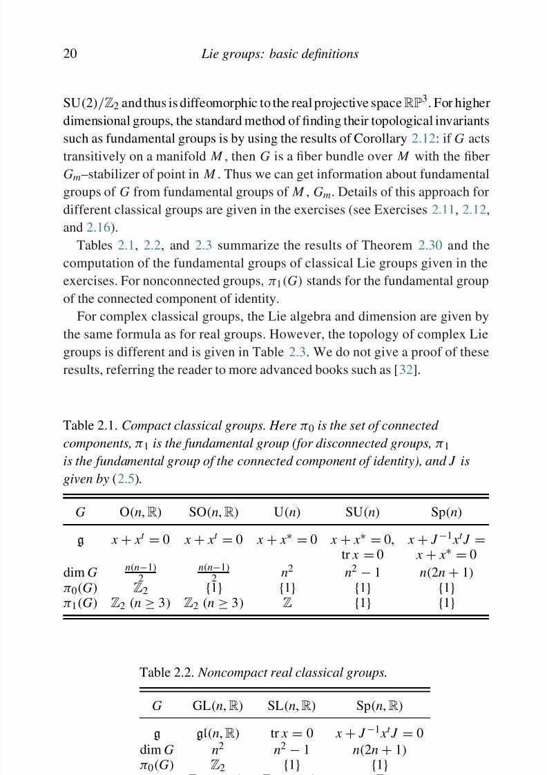
Tables 2.1, 2.2, and 2.3 summarize the results of Theorem 2.30 and the
computation of the fundamental groups of classical Lie groups given in the
exercises. For nonconnected groups, π1(G) stands for the fundamental group
of the connected component of identity.
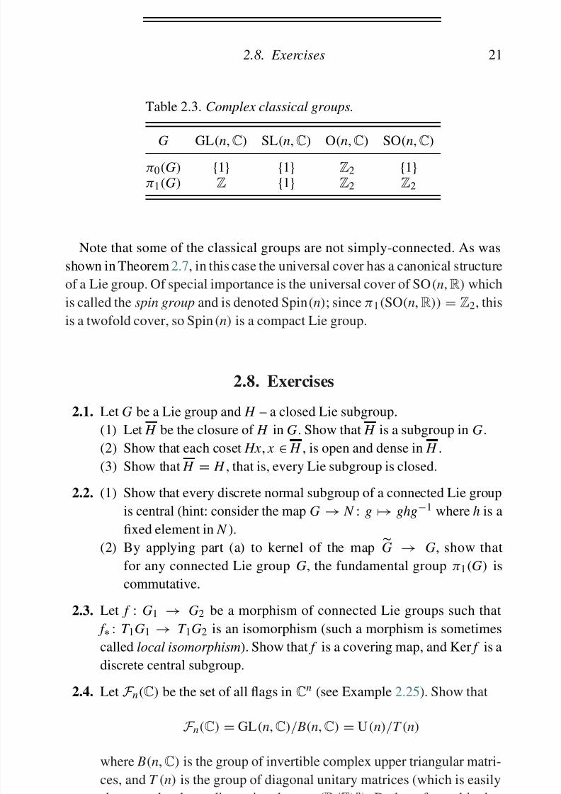
For complex classical groups, the Lie algebra and dimension are given by
the same formula as for real groups. However, the topology of complex Lie
groups is different and is given in Table 2.3. We do not give a proof of these
results, referring the reader to more advanced books such as [32].
Table 2.1. Compact classical groups. Here π0 is the set of connected
components, π1 is the fundamental group (for disconnected groups, π1
is the fundamental group of the connected component of identity), and J is
given by (2.5).
G O(n,R) SO(n,R) U(n) SU(n) Sp(n)
g x + x t
= 0 x + x t
= 0 x + x ∗ = 0 x + x ∗ = 0, x + J −1
x t
J =tr x = 0 x + x ∗ = 0
dim G n(n−1)
2n(n−1)
2 n2 n2 − 1 n(2n + 1)
π0(G) Z2 {1} {1} {1} {1}π1(G) Z2 (n ≥ 3) Z2 (n ≥ 3) Z {1} {1}
Table 2.2. Noncompact real classical groups.
G GL( R) SL( R) S ( R)
8/21/2019 Introduction to Lie Groups and Lie Algebras
http://slidepdf.com/reader/full/introduction-to-lie-groups-and-lie-algebras 33/236
2.8. Exercises 21
Table 2.3. Complex classical groups.
G GL(n,C) SL(n,C) O(n,C) SO(n,C)
π0(G) {1} {1} Z2 {1}π1(G) Z {1} Z2 Z2
Note that some of the classical groups are not simply-connected. As was
shown in Theorem 2.7, in this case the universal cover has a canonical structure
of a Lie group. Of special importance is the universal cover of SO(n,R) which
is called the spin group and is denoted Spin(n); since π1(SO(n,R)) = Z2, this
is a twofold cover, so Spin(n) is a compact Lie group.
2.8. Exercises
2.1. Let G be a Lie group and H – a closed Lie subgroup.(1) Let H be the closure of H in G. Show that H is a subgroup in G.
(2) Show that each coset Hx , x ∈ H , is open and dense in H .
(3) Show that H = H , that is, every Lie subgroup is closed.
2.2. (1) Show that every discrete normal subgroup of a connected Lie group
is central (hint: consider the map G → N : g → ghg−1 where h is a
fixed element in N ).
(2) By applying part (a) to kernel of the map G → G, show that
for any connected Lie group G, the fundamental group π1(G) is
commutative.
2.3. Let f : G1 → G2 be a morphism of connected Lie groups such that
f ∗ : T 1G1 → T 1G2 is an isomorphism (such a morphism is sometimes
called local isomorphism). Show that f is a covering map, and Ker f is a
discrete central subgroup.
2.4. Let F n(C) be the set of all flags in Cn
(see Example 2.25). Show that

8/21/2019 Introduction to Lie Groups and Lie Algebras
http://slidepdf.com/reader/full/introduction-to-lie-groups-and-lie-algebras 34/236
22 Lie groups: basic definitions
2.5. Let Gn,k be the set of all dimension k subspaces in Rn (usually called
the Grassmanian). Show that Gn,k is a homogeneous space for the
group O(n,R) and thus can be identified with coset space O(n,R)/ H
for appropriate H . Use it to prove that Gn,k is a manifold and find its
dimension.
2.6. Show that if G = GL(n,R) ⊂ End(Rn) so that each tangent space is
canonically identified with End(Rn),then ( Lg )∗v = gv where the product
in the right-hand side is the usual product of matrices, and similarly for
the right action. Also, the adjoint action is given by Ad g(v) = gvg−1.
Exercises 2.7–2.10 are about the group SU(2) and its adjoint
representation
2.7. Define a bilinear form on su(2) by (a, b) = 12
tr(abt ). Show that this form
is symmetric, positive definite, and invariant under the adjoint action of
SU(2).
2.8. Define a basis in su(2) by
iσ 1 = 0 i
i 0 iσ 2 = 0 1
−1 0 iσ 3 = i 0
0 −i
Show that the map
ϕ : SU(2) → GL(3,R)
g → matrix of Ad g in the basis iσ 1, iσ 2, iσ 3(2.8)
gives a morphism of Lie groups SU(2) → SO(3,R).
2.9. Let ϕ : SU(2) → SO(3,R) be the morphism defined in the previous
problem. Compute explicitly the map of tangent spaces ϕ∗ : su(2) → so(3,R) and show that ϕ∗ is an isomorphism. Deduce from this that
Ker ϕ is a discrete normal subgroup in SU(2), and that Im ϕ is an open
subgroup in SO(3,R).
2.10. Prove that the map ϕ used in two previous exercises establishes an
isomorphism SU(2)/Z2 → SO(3,R) and thus, since SU(2) S 3,
SO(3 R) RP3

8/21/2019 Introduction to Lie Groups and Lie Algebras
http://slidepdf.com/reader/full/introduction-to-lie-groups-and-lie-algebras 35/236
2.8. Exercises 23
2.12. Using Example 2.24, show that for n ≥ 2, we have π0(SO(n + 1,R)) =π0(SO(n,R)) and deduce from it that groups SO(n) are connected for all
n ≥ 2. Similarly, show that for n ≥ 3, π1(SO(n+1,R)) = π1(SO(n,R))
and deduce from it that for n ≥ 3, π1(SO(n,R)) = Z2.
2.13. Using the Gram–Schmidt orthogonalization process, show that
GL(n,R)/O(n,R) is diffeomorphic to the space of upper-triangular
matrices with positive entries on the diagonal. Deduce from this that
GL(n,R) is homotopic (as a topological space) to O(n,R).
2.14. Let Ln be the set of all Lagrangian subspaces in R2n with the standard
symplectic form ω defined in Section 2.7. (A subspace V is Lagrangian
if dim V = n and ω ( x , y) = 0 for any x , y ∈ V .)
Show that the group Sp(n,R) acts transitively on Ln and use it to define
on Ln a structure of a smooth manifold and find its dimension.
2.15. LetH = {a + bi + cj + dk | a, b, c, d ∈ R} be the algebra of quaternions,
defined by ij = k = − ji, jk = i = −kj, ki = j = −ik , i2 = j2 = k 2 =
−1, and let Hn
= {(h1, . . . , hn)
| hi
∈ H
}. In particular, the subalgebra
generated by 1, i coincides with the field C of complex numbers.
Note that Hn has a structure of both left and right module over H
defined by
h(h1, . . . , hn) = (hh1, . . . , hhn), (h1, . . . , hn)h = (h1h, . . . , hnh)
(1) Let EndH(Hn) be the algebra of endomorphisms of Hn considered
as right H-module:
EndH(Hn) = { A : Hn → Hn | A(h + h)
= A(h) + A(h), A(hh) = A(h)h}
Show that EndH(Hn) is naturally identified with the algebra of n × n
matrices with quaternion entries.
(2) Define anH–valued form ( , ) on Hn by
(h, h) = hihi

8/21/2019 Introduction to Lie Groups and Lie Algebras
http://slidepdf.com/reader/full/introduction-to-lie-groups-and-lie-algebras 36/236
24 Lie groups: basic definitions
Show that this is indeed a group and that a matrix A is in U(n,H) iff
A∗ A =
1, where ( A∗)ij
= A ji.
(3) Define a map C2n Hn by
( z1, . . . , z2n) → ( z1 + jzn+1, . . . , zn + jz2n)
Show that it is an isomorphism of complex vector spaces (if we con-
siderHn as a complex vector space by z(h1, . . . hn) = (h1 z, . . . , hn z))
and that this isomorphism identifies
EndH(Hn) = { A ∈ EndC(C2n) | A = J −1 AJ }
where J is defined by (2.5). (Hint: use jz = z j for any z ∈ C to show
that h → h j is identified with z → J z.)
(4) Show that under identification C2n Hn defined above, the
quaternionic form ( , ) is identified with
(z, z)−
j
z, z
where (z, z) = zi zi is the standard Hermitian form in C2n
and z, z = ni=1( zi+n z
i − zi z
i+n) is the standard bilinear skew-
symmetric form in C2n. Deduce from this that the group U(n,H) is
identified with Sp(n) = Sp(n,C) ∩ SU(2n).
2.16. (1) Show that Sp(1) SU(2) S 3.
(2) Using the previous exercise, show that we have a natural transitive
action of Sp(n) on the sphere S 4n−1 and a stabilizer of a point is
isomorphic to Sp(n − 1).
(3) Deduce that π1(Sp(n + 1)) = π1(Sp(n)), π0(Sp(n + 1)) =π0(Sp(n)).
8/21/2019 Introduction to Lie Groups and Lie Algebras
http://slidepdf.com/reader/full/introduction-to-lie-groups-and-lie-algebras 37/236
3
Lie groups and Lie algebras
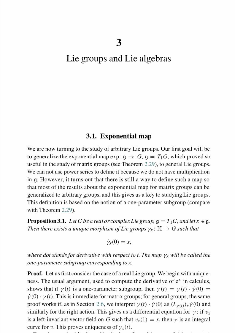
3.1. Exponential map
We are now turning to the study of arbitrary Lie groups. Our first goal will be
to generalize the exponential map exp: g → G, g = T 1G, which proved so
useful in the study of matrix groups (see Theorem 2.29), to general Lie groups.
We can not use power series to define it because we do not have multiplicationin g. However, it turns out that there is still a way to define such a map so
that most of the results about the exponential map for matrix groups can be
generalized to arbitrary groups, and this gives us a key to studying Lie groups.
This definition is based on the notion of a one-parameter subgroup (compare
with Theorem 2.29).
Proposition 3.1. Let G be a real or complex Lie group, g = T 1G, and let x ∈ g.
Then there exists a unique morphism of Lie groups γ x : K
→ G such that
γ x (0) = x ,
where dot stands for derivative with respect to t. The map γ x will be called the
one-parameter subgroup corresponding to x.
Proof. Let us first consider the case of a real Lie group. We begin with unique-
ness. The usual argument, used to compute the derivative of e x in calculus,
shows that if γ (t ) is a one-parameter subgroup, then γ (t ) = γ (t ) · γ (0) =γ (0) · γ (t ). This is immediate for matrix groups; for general groups, the same
f k if i S i 2 6 i ( ) ˙ (0) (L ) ˙ (0) d
8/21/2019 Introduction to Lie Groups and Lie Algebras
http://slidepdf.com/reader/full/introduction-to-lie-groups-and-lie-algebras 38/236
26 Lie groups and Lie algebras
the flow operator is also left-invariant: t (g1g2) = g1t (g2). Now let γ (t ) =t (1). Then γ (t
+s)
= t +s(1)
= s(t (1))
= s(γ (t )
·1)
= γ (t )s(1)
=γ (t )γ (s) as desired. This proves the existence of γ for small enough t . The fact
that it can be extended to any t ∈ R is obvious from γ (t + s) = γ (t )γ (s).
The proof for complex Lie groups is similar but uses generalization of the
usual results of the theory of differential equations to complex setup (such as
defining “time t flow” for complex time t ).
Note that a one-parameter subgroup may not be a closed Lie subgroup (as
is easy to see from Example 2.13); however, it will always be a Lie subgroup
in G.
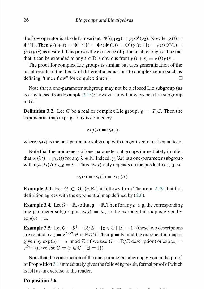
Definition 3.2. Let G be a real or complex Lie group, g = T 1G. Then the
exponential map exp: g → G is defined by
exp( x ) = γ x (1),
where γ x (t ) is the one-parameter subgroup with tangent vector at 1 equal to x .
Note that the uniqueness of one-parameter subgroups immediately impliesthat γ x (λt ) = γ λ x (t ) for any λ ∈ K. Indeed, γ x (λt ) is a one-parameter subgroup
with dγ x (λt )/dt |t =0 = λ x . Thus, γ x (t ) only depends on the product tx ∈ g, so
γ x (t ) = γ tx (1) = exp(tx ).
Example 3.3. For G ⊂ GL(n,K), it follows from Theorem 2.29 that this
definition agrees with the exponential map defined by (2.6).
Example 3.4. Let G = R,sothat g = R.Thenforany a ∈ g, the corresponding
one-parameter subgroup is γ a(t ) = ta, so the exponential map is given by
exp(a) = a.
Example 3.5. Let G = S 1 = R/Z = { z ∈ C | | z| = 1} (these two descriptions
are related by z = e2π iθ , θ ∈ R/Z). Then g = R, and the exponential map is
given by exp(a) = a mod Z (if we use G = R/Z description) or exp(a) =e2π ia (if we use G
= { z
∈C
| | z
| = 1
}).
Note that the construction of the one-parameter subgroup given in the proof
f i i 3 1 i di l i h f ll i l f l f f hi h
8/21/2019 Introduction to Lie Groups and Lie Algebras
http://slidepdf.com/reader/full/introduction-to-lie-groups-and-lie-algebras 39/236
3.1. Exponential map 27
(2) Let v be a right-invariant vector field on G. Then the time t flow of this
vector field is given by g
→ exp(tx )g, where x
= v(1).
The following theorem summarizes properties of the exponential map.
Theorem 3.7. Let G be a real or complex Lie group and g = T 1G.
(1) exp( x ) = 1 + x + . . . (that is, exp(0) = 1 and exp∗(0) : g → T 1G = g is
the identity map).
(2) The exponential map is a diffeomorphism ( for complex G, invertible ana-
lytic map) between some neighborhood of 0 in g and a neighborhood of 1
in G. The local inverse map will be denoted by log.
(3) exp((t + s) x ) = exp(tx ) exp(sx ) for any s, t ∈ K.
(4) For any morphism of Lie groups ϕ : G1 → G2 and any x ∈ g1 , we have
exp(ϕ∗( x )) = ϕ(exp( x )).
(5) For any X ∈ G, y ∈ g , we have X exp( y) X −1 = exp(Ad X . y) , where Ad
is the adjoint action of G on g defined by (2.4).
Proof. The first statement is immediate from the definition. Differenti-
ability (respectively, analyticity) of exp follows from the construction of γ x
given in the proof of Proposition 3.1 and general results about the depen-
dence of a solution of a differential equation on initial condition. The
fact that exp is locally invertible follows from (1) and inverse function
theorem.
The third statement is again an immediate corollary of the definition (exp(tx )
is a one-parameter subgroup in G).
Statement 4 follows from the uniqueness of one-parameter subgroup. Indeed,ϕ(exp(tx )) is a one-parameter subgroup in G2 with tangent vector at identity
ϕ∗(exp∗( x )) = ϕ∗( x ). Thus, ϕ (exp(tx )) = exp(t ϕ∗( x )).
The last statement is a special case of the previous one: the map Y → XYX −1
is a morphism of Lie groups G → G.
Comparing this with Theorem 2.29, we see that we have many of the
same results. A notable exception is that we have no analog of the state-
ment that if xy = yx , then exp( x ) exp( y) = exp( y) exp( x ). In fact thestatement does not make sense for general groups, as the product xy
8/21/2019 Introduction to Lie Groups and Lie Algebras
http://slidepdf.com/reader/full/introduction-to-lie-groups-and-lie-algebras 40/236
28 Lie groups and Lie algebras
Proposition 3.9. LetG1, G2 be Lie groups (real or complex ). I f G1 is connected,
then any Lie group morphism ϕ : G1
→ G2 is uniquely determined by the linear
map ϕ∗ : T 1G1 → T 1G2.
Proof. By Theorem 3.7, ϕ(exp x ) = exp(ϕ∗( x )). Since the image of the expo-
nential map contains a neighborhood of identity in G1, this implies that ϕ∗determines ϕ in a neighborhood of identity in G1. But by Corollary 2.10, any
neighborhood of the identity generates G1.
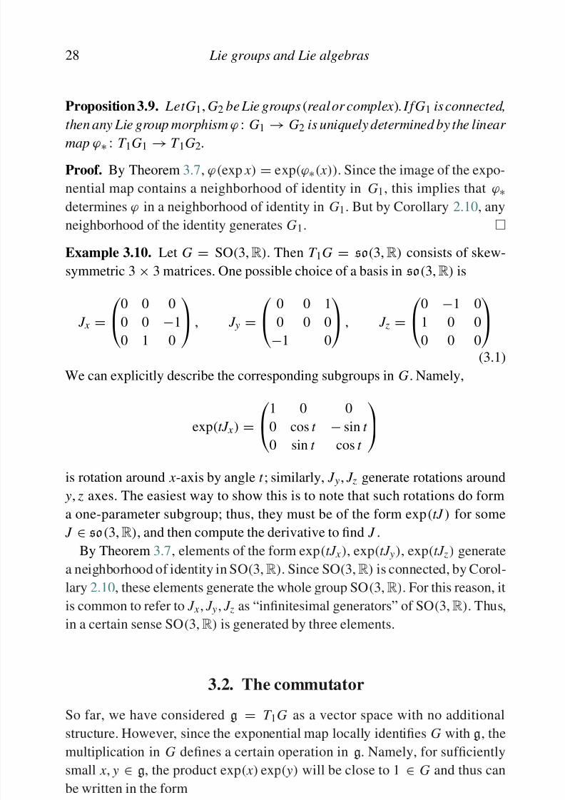
Example 3.10. Let G = SO(3,R). Then T 1G = so(3,R) consists of skew-
symmetric 3×
3 matrices. One possible choice of a basis in so(3,R) is
J x =0 0 0
0 0 −1
0 1 0
, J y = 0 0 1
0 0 0
−1 0
, J z =0 −1 0
1 0 0
0 0 0
(3.1)
We can explicitly describe the corresponding subgroups in G. Namely,
exp(tJ x ) = 1 0 0
0 cos t − sin t
0 sin t cos t
is rotation around x -axis by angle t ; similarly, J y, J z generate rotations around
y, z axes. The easiest way to show this is to note that such rotations do form
a one-parameter subgroup; thus, they must be of the form exp(tJ ) for some
J ∈ so(3,R), and then compute the derivative to find J .
By Theorem 3.7, elements of the form exp(tJ x ), exp(tJ y), exp(tJ z) generate
a neighborhood of identity in SO(3,R). Since SO(3,R) is connected, by Corol-
lary 2.10, these elements generate the whole group SO(3,R). For this reason, it
is common to refer to J x , J y, J z as “infinitesimal generators” of SO(3,R). Thus,
in a certain sense SO(3,R) is generated by three elements.
3.2. The commutator
So far, we have considered g = T 1G as a vector space with no additional
8/21/2019 Introduction to Lie Groups and Lie Algebras
http://slidepdf.com/reader/full/introduction-to-lie-groups-and-lie-algebras 41/236
3.2. The commutator 29
for some smooth (for complex Lie groups, complex analytic) map µ : g×g → g
defined in a neighborhood of (0, 0). The map µ is sometimes called the group
law in logarithmic coordinates.
Lemma 3.11. The Taylor series for µ is given by
µ( x , y) = x + y + λ( x , y) + · · ·
where dots stand for the terms of order ≥ 3 and λ : g × g → g is a bilinear
skew-symmetric (that is, satisfying λ( x , y) = −λ( y, x )) map.
Proof. Any smooth map can be written in the form α1( x ) + α2( y) + Q1( x ) +Q2( y) + λ( x , y) + · · · , where α1, α2 are linear maps g → g, Q1, Q2 are
quadratic, and λ is bilinear. Letting y = 0, we see that µ( x , 0) = x , which gives
α1( x ) = x , Q1( x ) = 0; similar argument shows that α2( y) = y, Q2( y) = 0.
Thus, µ( x , y) = x + y + λ( x , y) + · · · .
To show that λ is skew-symmetric, it suffices to check that λ( x , x ) = 0. But
exp( x ) exp( x ) = exp(2 x ), so µ( x , x ) = x + x .
For reasons that will be clear in the future, it is traditional to introduce notation[ x , y] = 2λ( x , y), so we have
exp( x ) exp( y) = exp( x + y + 1
2[ x , y] + · · · ) (3.2)
for some bilinear skew-symmetric map [ , ] : g×g → g. This map is called the
commutator .
Thus, we see that for any Lie group, its tangent space at identity g = T 1G
has a canonical skew-symmetric bilinear operation, which appears as the lowestnon-trivial term of the Taylor series for multiplication in G. This operation has
the following properties.
Proposition 3.12.
(1) Let ϕ : G1 → G2 be a morphism of real or complex Lie groups and
ϕ∗ : g1 → g2 , where g1 = T 1G1 , g2 = T 1G2 – the corresponding map
of tangent spaces at identity. Then ϕ
∗ preserves the commutator:
ϕ∗[ x , y] = [ϕ∗ x , ϕ∗ y] for any x , y ∈ g1.
8/21/2019 Introduction to Lie Groups and Lie Algebras
http://slidepdf.com/reader/full/introduction-to-lie-groups-and-lie-algebras 42/236
30 Lie groups and Lie algebras
Proof. The first statement is immediate from the definition of commutator (3.2)
and the fact that every morphism of Lie groups commutes with the exponential
map (Theorem 3.7). The second follows from the first and the fact that for any
g ∈ G, the map Ad g : G → G is a morphism of Lie groups.
The last formula is proved by explicit computation using (3.2).
This theorem shows that the commutator ing is closely related with the group
commutator in G, which explains the name.
Corollary 3.13. If G is a commutative Lie group, then [ x , y] = 0 for all x , y ∈ g.
Example 3.14. Let G ⊂ GL(n,K), so that g ⊂ gl(n,K). Then the commutator
is given by [ x , y] = xy − yx . Indeed, using (3.3) and keeping only linear and
bilinear terms, we can write (1+ x +· · · )(1+ y+· · · )(1− x +· · · )(1− y+· · · ) =1 + [ x , y] + · · · which gives [ x , y] = xy − yx .
3.3. Jacobi identity and the definition of a Lie algebra
So far, for a Lie group G, we have defined a bilinear operation on g = T 1G,
which is obtained from the multiplication on G. An obvious question is whether
the associativity of multiplication gives some identities for the commutator. In
this section we will answer this question; as one might expect, the answer is
“yes”.
By results of Proposition 3.12, any morphism ϕ of Lie groups gives rise
to a map ϕ
∗ of corresponding tangent spaces at identity which preserves the
commutator. Let us apply it to the adjoint action defined in Section 2.6, whichcan be considered as a morphism of Lie groups
Ad : G → GL(g). (3.4)
Lemma 3.15. Denote by ad = Ad∗ : g → gl(g) the map of tangent spaces
corresponding to the map (3.4). Then
(1) ad x . y = [ x , y](2) Ad(exp x ) = exp(ad x ) as operators g → g.
8/21/2019 Introduction to Lie Groups and Lie Algebras
http://slidepdf.com/reader/full/introduction-to-lie-groups-and-lie-algebras 43/236
3.3. Jacobi identity and the definition of a Lie algebra 31
On the other hand, by (3.3), exp(sx ) exp(ty) exp(−sx ) = exp(ty + ts[ x , y] +
· · ·). Combining these two results, we see that ad x . y
= [ x , y
].
The second part is immediate from Theorem 3.7.
Theorem 3.16. Let G be a real or complex Lie group, g = T 1G and let the
commutator [ , ] : g× g → g be defined by (3.2). Then it satisfies the following
identity, called Jacobi identity:
[ x , [ y, z]] = [[ x , y], z] + [ y, [ x , z]]. (3.5)
This identity can also be written in any of the following equivalent forms:
[ x , [ y, z] ]+ [ y, [ z, x ] ]+ [ z, [ x , y]] = 0
ad x .[ y, z] = [ad x . y, z] + [ y, ad x . z]ad[ x , y] = ad x ad y − ad y ad x .
(3.6)
Proof. Since Ad is a morphism of Lie groups G
→ GL(g), by Proposition 3.12,
ad : g → gl(g) must preserve commutator. But the commutator ingl(g) is given
by [ A, B] = AB − BA (see Example 3.14), so ad[ x , y] = ad x ad y − ad y ad x ,
which proves the last formula of (3.6).
Equivalence of all forms of Jacobi identity is left as an exercise to the reader
(see Exercise 3.3).
Definition 3.17. A Lie algebra over a field K is a vector space g over K with
a K-bilinear map
[,
]: g
×g
→ g which is skew-symmetric:
[ x , y
] = −[ y, x
]and satisfies Jacobi identity (3.5).
A morphism of Lie algebras is a K-linear map f : g1 → g2 which preserves
the commutator.
This definition makes sense for any field; however, in this book we will only
consider real (K = R) and complex (K = C) Lie algebras.
Example 3.18. Let g be a vector space with the commutator defined by
[ x , y] = 0 for all x , y ∈ g. Then g is a Lie algebra; such a Lie algebra is calledcommutative, or abelian, Lie algebra. This is motivated by Corollary 3.13,

8/21/2019 Introduction to Lie Groups and Lie Algebras
http://slidepdf.com/reader/full/introduction-to-lie-groups-and-lie-algebras 44/236
32 Lie groups and Lie algebras
defines on A a structure of a Lie algebra, which can be checked by a direct
computation.
Using the notion of a Lie algebra, we can summarize much of the results of
the previous two sections in the following theorem.
Theorem 3.20. Let G be a real or complex Lie group. Then g = T 1G has a
canonical structure of a Lie algebra over K with the commutator defined by
(3.2); we will denote this Lie algebra by Lie(G).
Every morphism of Lie groups ϕ : G1 → G2 defines a morphism of Lie
algebras ϕ∗ : g1 → g2 , so we have a map Hom(G1, G2) → Hom(g1, g2); if G1is connected, then this map is injective: Hom(G1, G2) ⊂ Hom(g1, g2).
3.4. Subalgebras, ideals, and center
In the previous section, we have shown that for every Lie group G the vector
space g
= T 1G has a canonical structure of a Lie algebra, and every morphism
of Lie groups gives rise to a morphism of Lie algebras.Continuing the study of this correspondence between groups and algebras,
we define analogs of Lie subgroups and normal subgroups.
Definition 3.21. Let g be a Lie algebra over K. A subspace h ⊂ g is called a
Lie subalgebra if it is closed under commutator, i.e. for any x , y ∈ h, we have
[ x , y] ∈ h. A subspace h ⊂ g is called an ideal if for any x ∈ g, y ∈ h, we have
[ x , y
] ∈ h.
It is easy to see that if h is an ideal, then g/h has a canonical structure of a
Lie algebra.
Theorem 3.22. Let G be a real or complex Lie group with Lie algebra g.
(1) Let H be a Lie subgroup in G (not necessarily closed ). Then h = T 1 H is a
Lie subalgebra in g.
(2) Let H be a normal closed Lie subgroup in G. Then h
= T 1 H is an ideal in
g , and Lie(G/ H ) = g/h.Conversely, if H is a closed Lie subgroup in G, such that H , G are
8/21/2019 Introduction to Lie Groups and Lie Algebras
http://slidepdf.com/reader/full/introduction-to-lie-groups-and-lie-algebras 45/236
3.5. Lie algebra of vector fields 33
Similarly, if H is a normal subgroup, then exp( x ) exp( y) exp(− x ) ∈ H for any
x
∈ g, y
∈ h, so the left-hand side of (3.3) is again in H . Identity Lie(G/ H )
=g/h follows from Theorem 2.11.
Finally, if h is an ideal in g, then it follows from Ad(exp( x )) = exp(ad x )
(Lemma 3.15) that for any x ∈ g, Ad(exp( x )) preserves h. Since expressions
of the form exp( x ), x ∈ g, generate G (Corollary 2.10), this shows that for any
g ∈ G, Ad g preserves h. Since by Theorem 3.7,
g exp( y)g−1 = exp(Ad g. y), g ∈ G, y ∈ g,
we see that for any y ∈ h, g exp( y)g−1 ∈ H . Since expressions exp y, y ∈ h,generate H , we see that ghg−1 ∈ H for any h ∈ H .
3.5. Lie algebra of vector fields
In this section, we illustrate the theory developed above in the example of the
group Diff ( M ) of diffeomorphisms of a manifold M . For simplicity, throughout
this section we only consider the case of real manifolds; however, all results
also hold for complex manifolds.
The group Diff ( M ) is not a Lie group (it is infinite-dimensional), but in many
ways it is similar to Lie groups. For example, it is easy to define what a smooth
map from some group G to Diff ( M ) is: it is the same as an action of G on M by
diffeomorphisms. Ignoring the technical problem with infinite-dimensionality
for now, let us try to see what is the natural analog of the Lie algebra for the
group Diff ( M ). It should be the tangent space at the identity; thus, its elements
are derivatives of one-parameter families of diffeomorphisms.
Let ϕt : M → M be a one-parameter family of diffeomorphisms. Then, for
every point m ∈ M , ϕt (m) is a curve in M and thus ddt
ϕt (m) ∈ T m M is a tangent
vector to M at m. In other words, ddt
ϕt is a vector field on M . Thus, it is natural
to define the Lie algebra of Diff ( M ) to be the space Vect( M ) of all smooth
vector fields on M .
What is the exponential map? If ξ ∈ Vect( M ) is a vector field, then exp(t ξ )
should be a one-parameter family of diffeomorphisms whose derivative isvector field ξ . So this is the solution of the differential equation

8/21/2019 Introduction to Lie Groups and Lie Algebras
http://slidepdf.com/reader/full/introduction-to-lie-groups-and-lie-algebras 46/236
34 Lie groups and Lie algebras
This may not be defined globally, but for the moment, let us ignore this
problem.
What is the commutator [ξ , η]? By (3.3), we need to consider t ξ sηt −ξ s−η.
It is well-known that this might not be the identity (if a plane flies 500 miles
north, then 500 miles west, then 500 miles south, then 500 miles east, then it
does not necessarily lands at the same spot it started – because Earth is not flat).
By analogy with (3.3), we expect that this expression can be written in the form
1+ ts[ξ , η]+ · · · for some vector field [ξ , η]. This is indeed so, as the following
proposition shows.
Proposition 3.23.
(1) Let ξ , η ∈ Vect( M ) be vector fields on M . Then there exists a unique vector
field which we will denote by [ξ , η] such that
t ξ
sηt
−ξ s−η = ts
[ξ ,η] + · · · , (3.8)
where dots stand for the terms of order 3 and higher in s, t.
(2) The commutator (3.8) defines on the space of vector fields a structure of an(infinite-dimensional) real Lie algebra.
(3) The commutator can also be defined by any of the following formulas:
[ξ , η] = d
dt (t
ξ )∗η (3.9)
∂[ξ ,η] f = ∂η(∂ξ f ) − ∂ξ (∂η f ), f ∈ C ∞( M ) (3.10)
f i∂i, g j∂ j = i, j(gi∂i( f j) − f i∂i(g j))∂ j (3.11)
where ∂ξ ( f ) is the derivative of a function f in the direction of the vector
field ξ , and ∂i = ∂∂ x i
for some local coordinate system { x i}.
The first two parts are, of course, to be expected, by analogy with finite-
dimensional situation. However, since Diff ( M ) is not a finite-dimensional Lie
group, we can not just refer to Theorem 3.20 but need to give a separate proof.
Such a proof, together with the proof of the last part, can be found in any goodbook on differential geometry, for example in [49].
8/21/2019 Introduction to Lie Groups and Lie Algebras
http://slidepdf.com/reader/full/introduction-to-lie-groups-and-lie-algebras 47/236
3.5. Lie algebra of vector fields 35
we use it. Thus, when using results from other books, be sure to double-check
which definition of commutator they use for vector fields.
The reason for the appearance of the minus sign is that the action of a diffeo-
morphism : M → M on functions on M is given by ( f )(m) = f (−1m)
(note the inverse!); thus, the derivative ∂ξ f = − ddt
t ξ f . For example, if
ξ = ∂ x is the constant vector field on R, then the flow on points is given
by t : x → x + t , and on functions it is given by (t f )( x ) = f ( x − t ), so
∂ x f = − ddt
t f .
Theorem 3.25. Let G be a finite-dimensional Lie group acting on a manifold
M , so we have a map ρ : G → Diff ( M ). Then
(1) This action defines a linear map ρ∗ : g → Vect( M ).
(2) The map ρ∗ is a morphism of Lie algebras: ρ∗[ x , y] = [ρ∗( x ), ρ∗( y)] , where
the commutator in the right-hand side is the commutator of vector fields.
If Diff ( M ) were a Lie group, this result would be a special case of Proposi-
tion 3.12. Since Diff ( M ) is not a Lie group, we need to give a separate proof,
suitably modifying the proof of Proposition 3.12. We leave this as an exerciseto the reader.
We will refer to the map ρ∗ : g → Vect( M ) as action of g by vector fields
on M .
Example 3.26. Consider the standard action of GL(n,R) on Rn. Considering
Rn as a manifold and forgetting the structure of a vector space, we see that
each element a
∈ gl(n,R) defines a vector field on Rn. An easy calculation
shows that this vector field is given by va( x ) = aij x j∂i, where x 1, . . . x n are
the coordinates of a point x in the standard basis of Rn, and ∂i = ∂∂ x i
.
Another important example is the action of G on itself by left multiplication.
Proposition 3.27. Consider the action of a Lie group G on itself by left mul-
tiplication: Lg.h = gh. Then for every x ∈ g , the corresponding vector field
ξ
= L
∗ x
∈ Vect(G) is the right-invariant vector field such that ξ (1)
= x.
Proof. Consider the one-parameter subgroup exp(tx ) ⊂ G. By Proposition 3.6,
8/21/2019 Introduction to Lie Groups and Lie Algebras
http://slidepdf.com/reader/full/introduction-to-lie-groups-and-lie-algebras 48/236
36 Lie groups and Lie algebras
3.6. Stabilizers and the center
Having developed the basic theory of Lie algebras, we can now go back toproving various results about Lie groups which were announced in Chapter 2,
such as proving that the stabilizer of a point is a closed Lie subgroup.
Theorem 3.29. Let G be a Lie group acting on a manifold M (respectively, a
complex Lie group holomorphically acting on a complex manifold M ) , and let
m ∈ M .
(1) The stabilizer Gm
= {g
∈ G
| gm
= m
}is a closed Lie subgroup in G, with
Lie algebra h = { x ∈ g | ρ∗( x )(m) = 0} , where ρ∗( x ) is the vector field on M corresponding to x.
(2) The map G/Gm → M given by g → g.m is an immersion. Thus, the
orbit Om = G · m is an immersed submanifold in M , with tangent space
T mO = g/h.
Proof. As in the proof of Theorem 2.30, it suffices to show that in some neigh-
borhood U of 1 ∈ G the intersection U ∩ Gm is a submanifold with tangent
space T 1Gm = h.It easily follows from (3.10) that h is closed under commutator, so it is a Lie
subalgebra in g. Also, since for x ∈ h, the corresponding vector field ξ = ρ∗( x )
vanishes at m, we have ρ (exp(th))(m) = t ξ (m) = m, so exp(th) ∈ Gm.
Now let us choose some vector subspace (not a subalgebra!) u ⊂ g which is
complementary to h: g = h ⊕ u. Since the kernel of the map ρ∗ : g → T m M is
h, the restriction of this map to u is injective. By implicit function theorem, this
implies that the map u
→ M : y
→ ρ(exp( y))(m) is injective for sufficiently
small y ∈ u, so exp( y) ∈ Gm ⇐⇒ y = 0.
Since in a sufficiently small neighborhood U of 1 in G, any element g ∈ U
can be uniquely written in the form exp( y) exp( x ), y ∈ u, x ∈ h (which follows
from inverse function theorem), and exp( y) exp( x )m = exp( y)m, we see that
g ∈ Gm ⇐⇒ g ∈ exp(h). Since exp h is a submanifold in a neighborhood of
1 ∈ G, we see that Gm is a submanifold.
The same proof also shows that we have an isomorphism T 1(G/Gm) = g/h u, so injectivity of the map ρ∗ : u → T m M shows that the map G/Gm → M isan immersion.
8/21/2019 Introduction to Lie Groups and Lie Algebras
http://slidepdf.com/reader/full/introduction-to-lie-groups-and-lie-algebras 49/236
3.6. Stabilizers and the center 37
is an immersion. If Im f is a submanifold and thus a closed Lie subgroup, we
have a Lie group isomorphism Im f
G1/ Ker f .
Proof. Consider the action of G1 on G2 given by ρ(g).h = f (g)h, g ∈ G1, h ∈G2. Then the stabilizer of 1 ∈ G2 is exactly Ker f , so by the previous theorem,
it is a closed Lie subgroup with Lie algebra Ker f ∗, and G1/ Ker f → G2 is an
immersion.
Corollary 3.31. Let V be a representation of a group G, and v ∈ V. Then the
stabilizer Gv is a closed Lie subgroup in G with Lie algebra { x ∈ g | x .v = 0}.
Example 3.32. Let V be a vector space over K with a bilinear form B, and let
O(V , B) = {g ∈ GL(V ) | B(g.v, g.w) = B(v, w) for all v, w}
be the group of symmetries of B. Then it is a Lie group over K with the Lie
algebra
o(V , B) = { x ∈ gl(V ) | B( x .v, w) + B(v, x .w) = 0 for all v, w}
Indeed, define the action of G on the space of bilinear forms by (gF )(v, w) =F (g−1.v, g−1.w). Then O(V , B) is exactly the stabilizer of B, so by Corol-
lary 3.31, it is a Lie group. Since the corresponding action of g is given by
( xF )(v, w) = −F ( x .v, w) − F (v, x .w) (which follows from Leibniz rule), we
get the formula for o(V , B).
As special cases, we recover the usual groups O(n,K) and Sp(n,K).
Example 3.33. Let A be a finite-dimensional associative algebra overK. Then
the group of all automorphisms of A
Aut( A) = {g ∈ GL( A) | (ga) · (gb) = g(a · b) for all a, b ∈ A}
is a Lie group with Lie algebra
Der( A) = { x ∈ gl( A) | ( x .a)b + a( x .b) = x .(ab) for all a, b ∈ A} (3.12)

8/21/2019 Introduction to Lie Groups and Lie Algebras
http://slidepdf.com/reader/full/introduction-to-lie-groups-and-lie-algebras 50/236
38 Lie groups and Lie algebras
The same argument also shows that for a finite-dimensional Lie algebra g,
the group
Aut(g) = {g ∈ GL(g) | [ga, gb] = g[a, b] for all a, b ∈ g} (3.13)
is a Lie group with Lie algebra
Der(g) = { x ∈ gl(g) | [ x .a, b] + [a, x .b] = x .[a, b] for all a, b ∈ g} (3.14)
called the Lie algebra of derivations of g. This algebra will play an important
role in the future.
Finally, we can show that the center of G is a closed Lie subgroup.
Definition 3.34. Let g be a Lie algebra. The center of g is defined by
z(g) = { x ∈ g | [ x , y] = 0 ∀ y ∈ g}.
Obviously, z(g) is an ideal in g.
Theorem 3.35. Let G be a connected Lie group. Then its center Z (G) is a
closed Lie subgroup with Lie algebra z(g).
Proof. Let g ∈ G, x ∈ g. It follows from the identity exp(Ad g.tx ) =g exp(tx )g−1 that g commutes with all elements of one-parameter subgroup
exp(tx ) iff Ad g. x = x . Since for a connected Lie group, elements of the form
exp(tx ) generate G , we see that g ∈ Z (G) ⇐⇒ Ad g. x = x for all x ∈ g. In
other words, Z (G)
= Ker Ad, where Ad : G
→ GL(g) is given by the adjoint
action. Now the result follows from Corollary 3.30.
The quotient group G/ Z (G) is usually called the adjoint group associated
with G and denoted Ad G:
Ad G = G/ Z (G) = Im(Ad : G → GL(g)) (3.15)
(for connected G). The corresponding Lie algebra is
ad g = g/ z(g) = Im(ad : g → gl(g)). (3.16)
8/21/2019 Introduction to Lie Groups and Lie Algebras
http://slidepdf.com/reader/full/introduction-to-lie-groups-and-lie-algebras 51/236
3.7. Campbell–Hausdorff formula 39
the lowest non-trivial term of the group law in logarithmic coordinates. Thus,
it might be expected that higher terms give more operations on g. However,
it turns out that it is not so: the whole group law is completely determined by
the lowest term, i.e. by the commutator. The following theorem gives the first
indication of this.
Theorem 3.36. Let x , y ∈ g be such that [ x , y] = 0. Then exp( x ) exp( y) =exp( x + y) = exp( y) exp( x ).
Proof. The most instructive (but not the easiest; see Exercise 3.12) way of
deducing this theorem is as follows. Let ξ , η be right-invariant vector fields
corresponding to x , y respectively, and let t ξ , t
η be time t flows of these vector
fields respectively (see Section 3.5). By Corollary 3.28, [ξ , η] = 0. By (3.9), it
implies that ddt
(t ξ )∗η = 0, which implies that (t
ξ )∗η = η, i.e. the flow of ξ
preserves field η. This, in turn, implies that t ξ commutes with the flow of field
η, so t ξ
sη−t
ξ = sη. Applying this to point 1 ∈ G and using Proposition 3.6,
we get exp(tx ) exp(sy) exp(−tx ) = exp(sy), so exp(tx ),exp(sy) commute for
all values of s, t .
In particular, this implies that exp(tx ) exp(ty) is a one-parameter subgroup;computing the tangent vector at t = 0, we see that exp(tx ) exp(ty) =exp(t ( x + y)).
In fact, similar ideas allow one to prove the following general statement,
known as the Campbell–Hausdorff formula.
Theorem 3.37. For small enough x , y ∈ g one has
exp( x ) exp( y) = exp(µ( x , y))
for some g-valued function µ( x , y) which is given by the following series
convergent in some neighborhood of (0, 0):
µ( x , y) = x + y +n≥2
µn( x , y), (3.17)
where µn( x , y) is a Lie polynomial in x , y of degree n, i.e. an expression con-
sisting of commutators of x , y, their commutators, etc., of total degree n in x , y.This expression is universal: it does not depend on the Lie algebra g or on the
8/21/2019 Introduction to Lie Groups and Lie Algebras
http://slidepdf.com/reader/full/introduction-to-lie-groups-and-lie-algebras 52/236
40 Lie groups and Lie algebras
The proof of this theorem is rather long. The key idea is writing the differential
equation for the function Z (t )
= µ(tx , y); the right-hand side of this equation
will be a power series of the form ant n(ad x )n y. Solving this differential
equation by power series gives the Campbell–Hausdorff formula. Details of
the proof can be found, for example, in [10, Section 1.6].
Corollary 3.38. The group operation in a connected Lie group G can be
recovered from the commutator in g = T 1G.
Indeed, locally the group law is determined by the Campbell–Hausdorff
formula, and G is generated by a neighborhood of 1.Note, however, that by itself this corollary does not allow us to recover the
group G from its Lie algebra g: it only allows us to determine the group law
provided that we already know the structure of G as a manifold.
3.8. Fundamental theorems of Lie theory
Let us summarize the results we have so far about the relation between Lie
groups and Lie algebras.
(1) Every real or complex Lie group G defines a Lie algebra g = T 1G (respec-
tively, real or complex), with commutator defined by (3.2); we will write
g = Lie(G). Every morphism of Lie groups ϕ : G1 → G2 defines a
morphism of Lie algebras ϕ∗ : g1 → g2. For connected G1, the map
Hom(G1, G2) → Hom(g1, g2)
ϕ → ϕ∗
is injective. (Here Hom(g1, g2) is the set of Lie algebra morphisms.)
(2) As a special case of the previous, every Lie subgroup H ⊂ G defines a Lie
subalgebra h ⊂ g.
(3) The group law in a connected Lie group G can be recovered from the
commutator ing; however, we do not yet know whether we can also recover
the topology of G from g

8/21/2019 Introduction to Lie Groups and Lie Algebras
http://slidepdf.com/reader/full/introduction-to-lie-groups-and-lie-algebras 53/236
3.8. Fundamental theorems of Lie theory 41
(2) Given a Lie subalgebra h ⊂ g = Lie(G), does there always exist a
corresponding Lie subgroup H
⊂ G?
(3) Can every Lie algebra be obtained as a Lie algebra of a Lie group?
As the following example shows, in this form the answer to question 1 is
negative.
Example 3.39. Let G1 = S 1 = R/Z, G2 = R. Then the Lie algebras are g1 =g2 = R with zero commutator. Consider the identity map g1 → g2 : a → a.
Then the corresponding morphism of Lie groups, if it exists, should be given by
θ → θ ; on the other hand, it must also satisfy f (Z
) = {0}. Thus, this morphismof Lie algebras can not be lifted to a morphism of Lie groups.
In this example the difficulty arose because G1 was not simply-connected. It
turns out that this is the only difficulty: after taking care of this, the answers to
all the questions posed above are positive. The following theorems give precise
statements.
Theorem 3.40. For any real or complex Lie group G, there is a bijection
between connected Lie subgroups H ⊂ G and Lie subalgebras h ⊂ g , given by H → h = Lie( H ) = T 1 H .
Theorem 3.41. If G1, G2 are Lie groups (real or complex ) and G1 is connected
and simply connected, then Hom(G1, G2) = Hom(g1, g2) , where g1, g2 are Lie
algebras of G1, G2 respectively.
Theorem 3.42 (Lie’s third theorem). Any finite-dimensional real or complex
Lie algebra is isomorphic to a Lie algebra of a Lie group (respectively, real or complex ).
Theorems 3.40–3.42 are the fundamental theorems of Lie theory; their proofs
are discussed below. In particular, combining these theorems with the previous
results, we get the following important corollary.
Corollary 3.43. For any real or complex finite-dimensional Lie algebra g ,
there is a unique (up to isomorphism) connected simply-connected Lie group
G (respectively, real or complex ) with Lie(G) = g. Any other connected Liegroup G with Lie algebra g must be of the form G/ Z for some discrete central
8/21/2019 Introduction to Lie Groups and Lie Algebras
http://slidepdf.com/reader/full/introduction-to-lie-groups-and-lie-algebras 54/236
42 Lie groups and Lie algebras
Lie algebra g, then there is a group homomorphism G → G which is locally
an isomorphism; thus, by results of Exercise 2.3, G
= G/ Z for some discrete
central subgroup Z .
Uniqueness of simply-connected group G now follows from π1(G/ Z ) = Z
(Theorem 2.7).
This corollary can be reformulated as follows.
Corollary 3.44. The categories of finite-dimensional Lie algebras and con-
nected, simply-connected Lie groups are equivalent.
We now turn to the discussion of the proofs of the fundamental theorems.
Proof of Theorem 3.42. The proof of this theorem is rather complicated and
full details will not be given here. The basic idea is to show that any Lie algebra
is isomorphic to a subalgebra in gl(n,K) (this statement is known as the Ado
theorem), after which we can use Theorem 3.40. However, the proof of the Ado
theorem is long and requires a lot of structure theory of Lie algebras, some of
which will be given in the subsequent chapters. The simplest case is when the
Lie algebra has no center (that is, ad x = 0 for all x ), then x → ad x gives anembedding g ⊂ gl(g). Proof of the general case can be found, e.g., in [24].
Proof of Theorem 3.41. We will show that this theorem follows from The-
orem 3.40. Indeed, we already discussed that any morphism of Lie groups
defines a morphism of Lie algebras and that for connected G1, the map
Hom(G1, G2) → Hom(g1, g2) is injective (see Theorem 3.20). Thus, it remains
to show that it is surjective, i.e. that every morphism of Lie algebras f : g1 → g2
can be lifted to a morphism of Lie groups ϕ : G1 → G2 with ϕ∗ = f .Define G = G1 × G2. Then the Lie algebra of G is g1 × g2. Let h =
{( x , f ( x )) | x ∈ g1} ⊂ g. This is a subalgebra: it is obviously a subspace, and
[( x , f ( x )), ( y, f ( y))] = ([ x , y], [ f ( x ), f ( y)]) = ([ x , y], f ([ x , y])) (the last identity
uses that f is a morphism of Lie algebras). Theorem 3.40 implies that there
is a corresponding connected Lie subgroup H → G1 × G2. Composing this
embedding with the projection p : G1 × G2 → G1, we get a morphism of Lie
groups π : H
→ G1, and π
∗: h
= Lie( H )
→ g1 is an isomorphism. By results
of Exercise 2.3, π is a covering map. On the other hand, G1 is simply-connected,and H is connected, so π must be an isomorphism. Thus, we have an inverse
8/21/2019 Introduction to Lie Groups and Lie Algebras
http://slidepdf.com/reader/full/introduction-to-lie-groups-and-lie-algebras 55/236
3.8. Fundamental theorems of Lie theory 43
Remark 3.45. In fact, the arguments above can be reversed to deduce Theo-
rem 3.40 from Theorem 3.41. For example, this is the way these theorems are
proved in [41].
Proof of Theorem 3.40. We will give the proof in the real case; proof in the
complex case is similar.
The proof we give here is based on the notion of integrable distribution.
For the reader’s convenience, we give the basic definitions here; details can be
found in [49] or [55].
A k -dimensional distribution on a manifold M is a k -dimensional subbundle
D ⊂ TM . In other words, at every point p ∈ M we have a k -dimensional
subspace D p ⊂ T p M , which smoothly depends on p. This is a generalization of
a well-known notion of direction field, commonly used in the theory of ordinary
differential equations. For a vector field v we will write v ∈ D if for every point
p we have v( p) ∈ D p.
An integral manifold for a distribution D is a k -dimensional submanifold
X ⊂ M such that at every point p ∈ X , we have T p X = D p. Again, this is a
straightforward generalization of the notion of an integral curve. However, fork > 1, existence of integral manifolds (even locally) is not automatic. We say
that a distribution D is completely integrable if for every p ∈ M , locally there
exists an integral manifold containing p (it is easy to show that such an integral
manifold is unique).
The following theorem gives a necessary and sufficient criterion of integr-
ability of a distribution.
Theorem 3.46 (Frobenius integrability criterion). A distribution D on M is
completely integrable if and only if for any two vector fields ξ , η ∈ D , one has
[ξ , η] ∈ D.
Proof of this theorem can be found in many books on differential geometry,
such as [49] and [55], and will not be repeated here.
Integrability is a local condition: it guarantees existence of an integral man-
ifold in a neighborhood of a given point. It is natural to ask whether this localintegral manifold can be extended to give a closed submanifold of M . The
f ll i h i h
8/21/2019 Introduction to Lie Groups and Lie Algebras
http://slidepdf.com/reader/full/introduction-to-lie-groups-and-lie-algebras 56/236
44 Lie groups and Lie algebras
Note, however, that the integral submanifold needs not be closed: in general,
it is not even an embedded submanifold but only an immersed one.
As before, we refer the reader to [49], [55] for the proof.
Let us now apply this theory to constructing, for a given Lie group G and
subalgebra h ⊂ g, the corresponding Lie subgroup H ⊂ G.
Notice that if such an H exists, then at every point p ∈ H , T p H = (T 1 H ) p =h. p (as in Section 2.6, we use notation v. p as a shorthand for ( R p−1 )∗v). Thus,
H will be an integral manifold of the distribution Dh defined by Dh
p = h. p. Let
us use this to construct H .
Lemma 3.48. For every point g ∈ G, there is locally an integral manifold of
the distribution Dh containing g, namely H 0 · g, where H 0 = exp u for some
neighborhood u of 0 in h.
This lemma can be easily proved using Frobenius theorem. Indeed, the
distribution Dh is generated by right-invariant vector fields corresponding to
elements of h. Since h is closed under [ , ], and commutator of right invariant
vector fields coincides with the commutator in g (Corollary 3.28), this shows
that the space of fields tangent to Dh is closed under the commutator, and thusDh is completely integrable.
To get an explicit description of the integral manifold, note that by Propo-
sition 3.6, the curve etx g for x ∈ h is the integral curve for a right invariant
vector field corresponding to x and thus this curve must be in the integral man-
ifold. Thus, for small enough x ∈ h, exp( x )g is in the integral manifold passing
through g . Comparing dimensions we get the statement of the lemma.
Alternatively, this lemma can also be proved without use of Frobenius
theorem but using the Campbell–Hausdorff formula instead.
Now that we have proved the lemma, we can construct the immersed sub-
group H as the maximal connected immersed integral manifold containing 1
(see Theorem 3.47). The only thing which remains to be shown is that H is a
subgroup. But since the distribution Dh is right-invariant, right action of G on
itself sends integral manifolds to integral manifolds; therefore, for any p ∈ H ,
H · p will be an integral manifold for Dh containing p. Since H itself also
contains p, we must have H · p = H , so H is a subgroup.
8/21/2019 Introduction to Lie Groups and Lie Algebras
http://slidepdf.com/reader/full/introduction-to-lie-groups-and-lie-algebras 57/236
3.9. Complex and real forms 45
Definition 3.49. Let g be a real Lie algebra. Its complexification is the complex
Lie algebra gC
= g
⊗R C
= g
⊕ ig with the obvious commutator. In this
situation, we will also say that g is a real form of gC.
In some cases, complexification is obvious: for example, if g = sl(n,R), then
gC = sl(n,C). The following important example, however, is less obvious.
Example 3.50. Let g = u(n). Then gC = gl(n,C).
Indeed, this immediately follows from the fact that any complex matrix can
be uniquely written as a sum of skew-Hermitian (i.e., from u(n)) and Hermitian
(iu(n)) matrices.
These notions can be extended to Lie groups. For simplicity, we only consider
the case of connected groups.
Definition 3.51. Let G be a connected complex Lie group, g = Lie(G) and let
K ⊂ G be a closed real Lie subgroup in G such that k = Lie(K ) is a real form
of g. Then K is called a real form of G.
It can be shown (see Exercise 3.15) that if g = Lie(G) is the Lie algebra of aconnected simply-connected complex Lie group G, then every real form k ⊂ g
can be obtained from a real form K ⊂ G of the Lie group.
Going in the opposite direction, from a real Lie group to a complex one, is
more subtle: there are real Lie groups that can not be obtained as real forms
of a complex Lie group (for example, it is known that the universal cover
of SL(2,R) is not a real form of any complex Lie group). It is still possible
to define a complexification GC for any real Lie group G; however, in general
G is not a subgroup of GC. Detailed discussion of this can be found in[15, Section I.7].
Example 3.52. The group G = SU(n) is a compact real form of the complex
group SL(n,C).
The operation of complexification, which is trivial at the level of Lie algebras,
is highly non-trivial at the level of Lie groups. Lie groups G and GC may be
topologically quite different: for example, SU(n) is compact while SL(n,C
) isnot. On the other hand, it is natural to expect – and is indeed so, as we will show
l h d h l b i i h i i li i

8/21/2019 Introduction to Lie Groups and Lie Algebras
http://slidepdf.com/reader/full/introduction-to-lie-groups-and-lie-algebras 58/236
46 Lie groups and Lie algebras
3.10. Example: so(3,R), su(2), and sl(2,C)
In this section, we bring together various explicit formulas related to Lie alge-bras so(3,R), su(2), sl(2,C). Most of these results have appeared before
in various examples and exercises; this section brings them together for the
reader’s convenience. This section contains no proofs: they are left to the reader
as exercises.
3.10.1. Basis and commutation relations
A basis in so(3,R) is given by
J x =0 0 0
0 0 −1
0 1 0
, J y = 0 0 1
0 0 0
−1 0 0
, J z =0 −1 0
1 0 0
0 0 0
(3.19)
The corresponding one-parameter subgroups in SO(3,R) are rotations: exp(tJ x )
is rotation by angle t around x -axis, and similarly for y, z.The commutation relations are given by
[ J x , J y] = J z, [ J y, J z] = J x , [ J z , J x ] = J y. (3.20)
A basis in su(2) is given by so-called Pauli matrices multiplied by i:
iσ 1 = 0 i
i 0 , iσ 2 = 0 1
−1 0 , iσ 3 = i 0
0 −i . (3.21)
The commutation relations are given by
[iσ 1, iσ 2] = −2iσ 3, [iσ 2, iσ 3] = −2iσ 1, [iσ 3, iσ 1] = −2iσ 2. (3.22)
Since sl(2,C) = su(2) ⊗ C, the same matrices can also be taken as a basis
of sl(2,C
). However, it is customary to use the following basis in sl(2,C
):0 1
0 0
1 0
8/21/2019 Introduction to Lie Groups and Lie Algebras
http://slidepdf.com/reader/full/introduction-to-lie-groups-and-lie-algebras 59/236
3.10. Example: so(3,R) , su(2) , and sl(2,C) 47
3.10.2. Invariant bilinear form
Each of these Lie algebras has an Ad G-invariant symmetric bilinear form. In
each case, it can be defined by ( x , y) = − tr( xy) (of course, it could also be
defined without the minus sign). For so(3,R), this form can also be rewritten
as ( x , y) = tr( xyt ); for su(n), as ( x , y) = tr( x yt ), which shows that in these two
cases this form is positive definite. In terms of bases defined above, it can be
written as follows:
• so(3,R): elements J x , J y, J z are orthogonal to each other, and ( J x , J x ) =( J y, J y)
= ( J z, J z)
= 2
• su(2): elements iσ k are orthogonal, and (iσ k , iσ k ) = 2.
• sl(2,C): (h, h) = −2, (e, f ) = ( f , e) = −1, all other products are zero.
3.10.3. Isomorphisms
We have an isomorphism of Lie algebras su(2) ∼−→ so(3,R) given by
iσ 1 → −
2 J x
iσ 2 → −2 J y (3.25)
iσ 3 → −2 J z .
It can be lifted to a morphism of Lie groups SU(2) → SO(3,R), which is a
twofold cover (see Exercise 2.8).
The inclusion su(2) ⊂ sl(2,C) gives an isomorphism su(2)C sl(2,C). In
terms of basis, it is given by
iσ 1 → i(e + f )
iσ 2 → e − f (3.26)
iσ 3 → ih.
Combining these two isomorphisms, we get an isomorphism so(3,R)C = so(3,C)
∼
−→ sl(2,C)
Jx → − i(e + f )
8/21/2019 Introduction to Lie Groups and Lie Algebras
http://slidepdf.com/reader/full/introduction-to-lie-groups-and-lie-algebras 60/236
48 Lie groups and Lie algebras
3.11. Exercises
3.1. Consider the group SL(2,R). Show that the element X = −1 1
0 −1is not in the image of the exponential map. (Hint: if X = exp( x ), what
are the eigenvalues of x ?).
3.2. Let f : g → G be any smooth map such that f (0) = 1, f ∗(0) = id; we
can view such a map as a local coordinate system near 1 ∈ G. Show
that the the group law written in this coordinate system has the form
f ( x ) f ( y)
= f ( x
+ y
+ B( x , y)
+· · ·) for some bilinear map B : g
⊗g
→ g
and that B( x , y) − B( y, x ) = [ x , y].
3.3. Show that all forms of Jacobi identity given in (3.5), (3.6) are equivalent.
3.4. Show that if we denote, for x ∈ g, by ξ x the left-invariant vector field on
G such that ξ x (1) = x (cf. Theorem 2.27), then [ξ x , ξ y] = −ξ [ x , y].
3.5. (1) Prove that R3 with the commutator given by the cross-product is a
Lie algebra. Show that this Lie algebra is isomorphic to so(3,R).
(2) Let ϕ : so(3,R) → R3
be the isomorphism of part (1). Provethat under this isomorphism, the standard action of so(3) on R3 is
identified with the action of R3 on itself given by the cross-product:
a · v = ϕ(a) × v, a ∈ so(3), v ∈ R3
where a · v is the usual multiplication of a matrix by a vector.
This problem explains a common use of cross-products in mechan-
ics (see, e.g. [1]): angular velocities and angular momenta are actuallyelements of Lie algebra so(3,R) (to be precise, angular momenta are
elements of the dual vector space, ( so(3,R)∗), but we can ignore this dif-
ference). To avoid explaining this, most textbooks write angular velocities
as vectors inR3 and use cross-product instead of commutator. Of course,
this would completely fail in dimensions other than 3, where so(n,R) is
not isomorphic to Rn even as a vector space.
3.6. Let Pn be the space of polynomials with real coefficients of degree ≤ nin variable x . The Lie group G = R acts on Pn by translations of the

8/21/2019 Introduction to Lie Groups and Lie Algebras
http://slidepdf.com/reader/full/introduction-to-lie-groups-and-lie-algebras 61/236
3.11. Exercises 49
3.7. Let G be the Lie group of all maps A : R → R having the form
A( x )
= ax
+b, a
= 0. Describe explicitly the corresponding Lie algebra.
[There are two ways to do this problem. The easy way is to embed
G ⊂ GL(2,R), which makes the problem trivial. A more straightforward
way is to explicitly construct some basis in the tangent space, construct
the corresponding one-parameter subgroups, and compute the commu-
tator using (3.3). The second way is recommended to those who want to
understand how the correspondence between Lie groups and Lie algebras
works.]
3.8. Let SL(2,C) act on CP1
in the usual way:a b
c d
( x : y) = (ax + by : cx + dy).
This defines an action of g = sl(2,C) by vector fields on CP1. Write
explicitly vector fields corresponding to h, e, f in terms of coordinate
t = x / y on the open cell C ⊂ CP1.
3.9. Let G be a Lie group with Lie algebra g, and Aut(g), Der(g) be as definedin Example 3.33.
(1) Show that g → Ad g gives a morphism of Lie groups G → Aut(G);
similarly, x → ad x is a morphism of Lie algebras g → Der g. (The
automorphisms of the form Ad g are called inner automorphisms;
the derivations of the form ad x , x ∈ g are called inner derivations.)
(2) Show that for f ∈ Der g, x ∈ g, one has [ f , ad x ] = ad f ( x ) as
operators in g, and deduce from this that ad(g) is an ideal in Der g.
3.10. Let { H α}α∈ A be some family of closed Lie subgroups in G , with the Lie
algebras hα = Lie( H α). Let H = α H α. Without using the theorem
about closed subgroup, show that H is a closed Lie subgroup with Lie
algebra h =α hα.
3.11. Let J x , J y, J z be the basis in so(3,R) described in Section 3.10. The stan-
dard action of SO(3,R) on R3 defines an action of so(3,R) by vector
fields onR3. Abusing the language, we will use the same notation J x
, J y
, J z
for the corresponding vector fields on R3. Let sph = J 2 x + J 2 y + J 2 z ; this
i d d diff i l R3 hi h i ll ll d h

8/21/2019 Introduction to Lie Groups and Lie Algebras
http://slidepdf.com/reader/full/introduction-to-lie-groups-and-lie-algebras 62/236
50 Lie groups and Lie algebras
(3) Show that the usual Laplace operator = ∂2 x +∂2
y +∂2 z can be written
in the form
= 1
r 2sph
+ radial , where radial is a differential
operator written in terms of r = x 2 + y2 + z2 and r ∂r = x ∂ x + y∂ y + z∂ z.
(4) Show that sph is rotation invariant: for any function f and g ∈SO(3,R), sph(gf ) = g(sph f ). (Later we will describe a better
way of doing this.)
3.12. Give an alternative proof of Theorem 3.36, using Lemma 3.15.
3.13. (1) Let g be a three-dimensional real Lie algebra with basis x , y, zand commutation relations [ x , y] = z, [ z, x ] = [ z, y] = 0 (this
algebra is called Heisenberg algebra). Without using the Campbell–
Hausdorff formula, show that in the corresponding Lie group, one
has exp(tx ) exp(sy) = exp(tsz) exp(sy) exp(tx ) and construct explic-
itly the connected, simply connected Lie group corresponding to
g.
(2) Generalize the previous part to the Lie algebra g
= V
⊕R z, where
V is a real vector space with non-degenerate skew-symmetric formω and the commutation relations are given by [v1, v2] = ω(v1, v2) z,
[ z, v] = 0.
3.14. This problem is for readers familiar with the mathematical formalism of
classical mechanics.
Let G be a real Lie group and A – a positive definite symmetric bilinear
form on g; such a form can also be considered as a linear map g → g∗.
(1) Let us extend A to a left invariant metric on G. Consider mechanicalsystem describing free motion of a particle on G, with kinetic energy
given by A(g, g) and zero potential energy. Show that equations of
motion for this system are given by Euler’s equations:
= ad∗ v.
where v = g−1g ∈ g, = Av ∈ g∗, and ad∗ is the coadjoint action:
ad∗ x . f , y = − f , ad x . y x , y ∈ g, f ∈ g∗.
8/21/2019 Introduction to Lie Groups and Lie Algebras
http://slidepdf.com/reader/full/introduction-to-lie-groups-and-lie-algebras 63/236
3.11. Exercises 51
(2) Using the results of the previous part, show that if A is a bi-invariant
metric on G, then one-parameter subgroups exp(tx ), x
∈ g are
geodesics for this metric.
3.15. Let G be a complex connected simply-connected Lie group, with Lie
algebra g = Lie(G), and let k ⊂ g be a real form of g.
(1) Define the R-linear map θ : g → g by θ ( x + i y) = x − i y, x , y ∈ k.
Show that θ is an automorphism of g (considered as a real Lie alge-
bra), and that it can be uniquely lifted to an automorphism θ : G → G
of the group G (considered as a real Lie group).
(2) Let K = Gθ . Show that K is a real Lie group with Lie algebra k.
3.16. Let Sp(n) be the unitary quaternionic group defined in Section 2.7. Show
that sp(n)C = sp(n,C). Thus Sp(n) is a compact real form of Sp(n,C).
3.17. Let so( p, q) = Lie(SO( p, q)). Show that its complexification is
so( p, q)C = so( p + q,C).
3.18. Let
S = 0 −
1
1 0 ∈ SL(2,C).
(1) Show that S = exp
π2
( f − e)
, where e, f ∈ sl(2,C) are defined by
(3.23).
(2) Compute Ad S in the basis e, f , h.
3.19. Let G be a complex connected Lie group.
(1) Show that g
→ Ad g is an analytic map G
→ gl(g).
(2) Assume that G is compact. Show that then Ad g = 1 for any g ∈ G.
(3) Show that any connected compact complex group must be commu-
tative.
(4) Show that if G is a connected complex compact group, then the
exponential map gives an isomorphism of Lie groups
g/ L G
for some lattice L ⊂ g (i.e. a free abelian group of rank equal to
2di )
8/21/2019 Introduction to Lie Groups and Lie Algebras
http://slidepdf.com/reader/full/introduction-to-lie-groups-and-lie-algebras 64/236
4
Representations of Lie groups andLie algebras
In this section, we will discuss the representation theory of Lie groups and Lie
algebras – as far as it can be discussed without using the structure theory of
semisimple Lie algebras. Unless specified otherwise, all Lie groups, algebras,
and representations are finite-dimensional, and all representations are complex.
Lie groups and Lie algebras can be either real or complex; unless specified
otherwise, all results are valid both for the real and complex case.
4.1. Basic definitions
Let us start by recalling the basic definitions.
Definition 4.1. A representation of a Lie group G is a vector space V together
with a morphism ρ : G
→ GL(V ).
A representation of a Lie algebra g is a vector space V together with amorphism ρ : g → gl(V ).
A morphism between two representations V , W of the same group G is a
linear map f : V → W which commutes with the action of G: f ρ (g) = ρ(g) f .
In a similar way one defines a morphism of representations of a Lie algebra.
The space of all G-morphisms (respectively, g-morphisms) between V and W
will be denoted by HomG(V , W ) (respectively, Homg(V , W )).
Remark 4.2. Morphisms between representations are also frequently calledintertwining operators because they “intertwine” action of G in V and W .

8/21/2019 Introduction to Lie Groups and Lie Algebras
http://slidepdf.com/reader/full/introduction-to-lie-groups-and-lie-algebras 65/236
4.1. Basic definitions 53
Note that in this definition we did not specify whether V and G, g are real or
complex. Usually if G (respectively, g) is complex, then V should also be taken
a complex vector space. However, it also makes sense to take complex V even
if G is real: in this case we require that the morphism G → GL(V ) be smooth,
considering GL(V ) as 2n2-dimensional real manifold. Similarly, for real Lie
algebras we can consider complex representations requiring that ρ : g → gl(V )
be R-linear.
Of course, we could also restrict ourselves to consideration of real represen-
tations of real groups. However, it turns out that the introduction of complex
representations significantly simplifies the theory even for real groups and alge-
bras. Thus, from now on, all representations will be complex unless specified
otherwise.
The first important result about representations of Lie groups and Lie algebras
is the following theorem.
Theorem 4.3. Let G be a Lie group (real or complex ) with Lie algebra g.
(1) Every representation ρ : G
→ GL(V ) defines a representation ρ
∗: g
→gl(V ) , and every morphism of representations of G is automatically a
morphism of representations of g.
(2) If G is connected, simply-connected, then ρ → ρ∗ gives an equivalence of
categories of representations of G and representations of g. In particular,
every representation of g can be uniquely lifted to a representation of G,
and HomG(V , W ) = Homg(V , W ).
Indeed, part (1) is a special case of Theorem 3.20, and part (2) follows from
Theorem 3.41.
This is an important result, as Lie algebras are, after all, finite dimensional
vector spaces, so they are easier to deal with. For example, this theorem shows
that a representation of SU(2) is the same as a representation of su(2), i.e. a vec-
tor space with three endomorphisms X , Y , Z , satisfying commutation relations
XY − YX = Z , YZ − ZY = X , ZX − XZ = Y .
This theorem can also be used to describe representations of a group which
is connected but not simply-connected: indeed, by Corollary 3.43 any suchgroup can be written as G = G/ Z for some simply-connected group G and
8/21/2019 Introduction to Lie Groups and Lie Algebras
http://slidepdf.com/reader/full/introduction-to-lie-groups-and-lie-algebras 66/236
54 Representations of Lie groups and Lie algebras
of representation of gC , and Homg(V , W ) = HomgC(V , W ). In other words,
categories of complex representations of g, gC are equivalent.
Proof. Let ρ : g → gl(V ) be the representation of g. Extend it to gC by ρ ( x +i y) = ρ( x ) + iρ( y). We leave it to the reader to check that so defined ρ is
complex-linear and agrees with the commutator.
Example 4.5. The categories of finite-dimensional representations of SL(2,C),
SU(2), sl(2,C) and su(2) are all equivalent. Indeed, by results of Section 3.10,
sl(2,C) = ( su(2))C, so categories of their finite-dimensional representations
are equivalent; since Lie groups SU(2), SL(2,C) are simply-connected, they
have the same representations as the corresponding Lie algebras.
This, in particular, allows us to reduce the problem of study of representa-
tions of a non-compact Lie group SL(2,C) to the study of representations of
a compact Lie group SU(2). This is useful because, as we will show below,
representation theory of compact Lie groups is especially nice.
Remark 4.6. This only works for finite-dimensional representations; the theory
of infinite-dimensional representations of SL(2,C) is very different from thatof SU(2).
The following are some examples of representations that can be defined for
any Lie group G (and thus, for any Lie algebra g).
Example 4.7. Trivial representation: V = C, ρ(g) = id for any g ∈ G
(respectively, ρ ( x ) = 0 for any x ∈ g).
Example 4.8. Adjoint representation: V = g, ρ(g) = Ad g (respectively,ρ( x ) = ad x ). See (2.4), Lemma 3.15 for definition of Ad, ad.
4.2. Operations on representations
In this section, we discuss basic notions of representation theory of Lie
groups and Lie algebras, giving examples of representations, operations on
representations such as direct sum and tensor product, and more.
4.2.1. Subrepresentations and quotients
8/21/2019 Introduction to Lie Groups and Lie Algebras
http://slidepdf.com/reader/full/introduction-to-lie-groups-and-lie-algebras 67/236
4.2. Operations on representations 55
It is trivial to check that if W ⊂ V is a subrepresentation, then the quotient
space V /W has a canonical sructure of a representation. It will be called factor
representation, or the quotient representation.
4.2.2. Direct sum and tensor product
Lemma 4.10. Let V , W be representations of G (respectively, g). Then there
is a canonical structure of a representation on V ∗ , V ⊕ W , V ⊗ W .
Proof. Action of G on V ⊕W is given by ρ (g)(v+w) = ρ(g)v + ρ(g)w (for
g
∈ G, v
∈ V , w
∈ W ) and similarly for g.
For tensor product, we define ρ(g)(v⊗w) = ρ(g)v⊗ ρ(g)w. However, the
action of g is trickier: indeed, naive definition ρ ( x )(v ⊗ w) = ρ( x )v ⊗ ρ( x )w
(for x ∈ g) does not define a representation (it is not even linear in x ). Instead,
if we write x = γ (0) for some one-parameter subgroup γ (t ) in the Lie group
G with γ (0) = 1, then
ρ( x )(v ⊗ w) = d
dt |t =0(γ (t )v ⊗ γ (t )w) = (γ (0)v ⊗ γ (0)w)
+ (γ (0)v ⊗ γ (t )w)
= ρ( x )v ⊗ w + v ⊗ ρ( x )w
by using Leibniz rule. Thus, we define for x ∈ g
ρ( x )(v ⊗ w) = ρ ( x )v ⊗ w + v ⊗ ρ( x )w.
It is easy to show, even without using the Lie group G, that so defined action is
indeed a representation of g on V ⊗ W .
To define the action of G, g on V ∗, we require that the natural pairing
V ⊗ V ∗ → C be a morphism of representations, considering C as the triv-
ial representation. This gives, for v ∈ V , v∗ ∈ V ∗, ρ(g)v, ρ(g)v∗ = v, v∗,
so the action of G in V ∗ is given by ρV ∗ (g) = ρ (g−1)t , where for A : V → V ,
we denote by At the adjoint operator V ∗ → V ∗.
Similarly, for the action of g we get ρ( x )v, v∗ + v, ρ( x )v∗ = 0, so
ρV ∗ ( x ) = −(ρV ( x ))t
.
As an immediate corollary, we see that for a representation V , any tensor
8/21/2019 Introduction to Lie Groups and Lie Algebras
http://slidepdf.com/reader/full/introduction-to-lie-groups-and-lie-algebras 68/236
56 Representations of Lie groups and Lie algebras
This representation is called the coadjoint representation and plays an important
role in representation theory: for example, for a large class of Lie algebras there
is a bijection between (some) G–orbits in g∗ and finite-dimensional irreducible
representations of g (see [30]).
Example 4.12. Let V be a representation of G (respectively, g). Then the
space End(V ) V ⊗ V ∗ of linear operators on V is also a representation,
with the action given by g : A → ρV (g) AρV (g−1) for g ∈ G (respectively,
x : A → ρV ( x ) A − AρV ( x ) for x ∈ g). More generally, the space of linear
maps Hom(V , W ) between two representations is also a representation with the
action defined by g : A → ρW (g) AρV (g−1) for g ∈ G (respectively, x : A →ρW ( x ) A − AρV ( x ) for x ∈ g).
Similarly, the space of bilinear forms on V is also a representation, with
action given by
gB(v, w) = B(g−1v, g−1
w), g ∈ G
xB(v, w) = −( B( x .v, w) + B(v, x .w)), x ∈ g.
Proof of these formulas is left to the reader as an exercise.
4.2.3. Invariants
Definition 4.13. Let V be a representation of a Lie group G. A vector v ∈ V is
called invariant if ρ (g)v = v for all g ∈ G. The subspace of invariant vectors
in V is denoted by V G.
Similarly, let V be a representation of a Lie algebra g. A vector v ∈ V is
called invariant if ρ( x )v = 0 for all x ∈ g. The subspace of invariant vectors
in V is denoted by V g.
We leave it to the reader to prove that if G is a connected Lie group with the
Lie algebra g, then for any representation V of G, we have V G = V g.
Example 4.14. Let V , W be representations and Hom(V , W ) be the space
of linear maps V
→ W , with the action of G defined as in Example 4.12.
Then (Hom(V , W ))G = HomG(V , W ) is the space of intertwining operators.In particular, this shows that V G = (Hom(C, V ))G = HomG(C, V ), with C
8/21/2019 Introduction to Lie Groups and Lie Algebras
http://slidepdf.com/reader/full/introduction-to-lie-groups-and-lie-algebras 69/236
4.3. Irreducible representations 57
for any g ∈ G, v, w ∈ V . Similarly, B is invariant under the action of g iff
B( x .v, w) + B(v, x .w) = 0
for any x ∈ g, v, w ∈ V .
We leave it to the reader to check that B is invariant iff the linear map V → V ∗defined by v → B(v, −) is a morphism of representations.
4.3. Irreducible representations
One of the main problems of the representation theory is the problem of classi-
fication of all representations of a Lie group or a Lie algebra. In this generality,
it is an extremely difficult problem and for a general Lie group, no satisfactory
answer is known. We will later show that for some special classes of Lie groups
(namely compact Lie groups and semisimple Lie groups, to be defined later)
this problem does have a good answer.
The most natural approach to this problem is to start by studying the sim-
plest possible representations, which would serve as building blocks for morecomplicated representations.
Definition 4.16. A non-zero representation V of G or g is called irreducible
or simple if it has no subrepresentations other than 0, V . Otherwise V is called
reducible.
Example 4.17. Space Cn, considered as a representation of SL(n,C), is
irreducible.
If a representation V is reducible, then it has a non-trivial subrepresentation
W and thus, V can be included in a short exact sequence 0 → W → V →V /W → 0; thus, in a certain sense it is built out of simpler pieces. The
natural question is whether this exact sequence splits, i.e. whether we can write
V = W ⊕ (V /W ) as a representation. If so then repeating this process, we can
write V as a direct sum of irreducible representations.
Definition 4.18. A representation is called completely reducible or semisimple
if it is isomorphic to a direct sum of irreducible representations: V V i, V i
irreducible.
8/21/2019 Introduction to Lie Groups and Lie Algebras
http://slidepdf.com/reader/full/introduction-to-lie-groups-and-lie-algebras 70/236
58 Representations of Lie groups and Lie algebras
Example 4.19. Let G = R, so g = R. Then a representation of g is the same
as a vector space V with a linear map R
→ End(V ); obviously, every such
map is of the form t → tA for some A ∈ End(V ) which can be arbitrary. The
corresponding representation of the group R is given by t → exp(tA). Thus,
classifying representations of R is equivalent to classifying linear maps V → V
up to a change of basis. Such a classification is known (Jordan normal form)
but non-trivial.
If v is an eigenvector of A then the one-dimensional space Cv ⊂ V is invari-
ant under A and thus a subrepresentation in V . Since every linear operator in
a complex vector space has an eigenvector, this shows that every representa-
tion of R is reducible, unless it is one-dimensional. Thus, the only irreducible
representations of R are one-dimensional.
Now one easily sees that writing a representation given by t → exp(tA) as
a direct sum of irreducible ones is equivalent to diagonalizing A. So a repre-
sentation is completely reducible iff A is diagonalizable. Since not every linear
operator is diagonalizable, not every representation is completely reducible.
Thus, more modest goals of the representation theory would be answeringthe following questions:
(1) For a given Lie group G, classify all irreducible representations of G.
(2) For a given representation V of a Lie group G, given that it is com-
pletely reducible, find explicitly the decomposition of V into direct sum
of irreducibles.
(3) For which Lie groups G all representations are completely reducible?
One tool which can be used in decomposing representations into direct sum
is the use of central elements.
Lemma 4.20. Let ρ : G → GL(V ) be a representation of G (respectively, g)
and A : V → V a diagonalizable intertwining operator. Let V λ ⊂ V be the
eigenspace for A with eigenvalue λ. Then each V λ is a subrepresentation, so
V =
V λ as a representation of G (respectively g).
The proof of this lemma is trivial and is left to the reader. As an immediate
8/21/2019 Introduction to Lie Groups and Lie Algebras
http://slidepdf.com/reader/full/introduction-to-lie-groups-and-lie-algebras 71/236
4.4. Intertwining operators and Schur’s lemma 59
Of course, there is no guarantee that V λ will be an irreducible representation;
moreover, in many cases the Lie groups we consider have no central elements
at all.
Example 4.22. Consider action of GL(n,C) onCn ⊗Cn. Then the permutation
operator P : v ⊗ w → w ⊗ v commutes with the action of GL(n,C), so the
subspaces S 2Cn, 2Cn of symmetric and skew-symmetric tensors (which are
exactly the eigenspaces of P) are GL(n,C)-invariant and Cn ⊗ Cn = S 2Cn ⊕2Cn as a representation. In fact, both S 2Cn, 2Cn are irreducible (this is
not obvious but can be proved by a lengthy explicit calculation; a better way
of proving this will be given in Exercise 8.4). Thus, Cn ⊗ Cn is completelyreducible.
4.4. Intertwining operators and Schur’s lemma
Recall that an intertwining operator is a linear map V → W which commutes
with the action of G. Such operators frequently appear in various applications.
A typical example is quantum mechanics, where we have a vector space V (describing the state space of some mechanical system) and the Hamiltonian
operator H : V → V . Then saying that this system has a symmetry described
by a group G is the same as saying that we have an action of G on V which
leaves H invariant, i.e. gHg−1 = H for any g ∈ G. This exactly means that
H is an intertwining operator. A real-life example of such situation (spherical
Laplace operator) will be described in Section 4.9.
These examples motivate the study of intertwining operators. For exam-
ple, does G-invariance of an operator helps computing eigenvalues andeigenspaces?
The first result in this direction is the following famous lemma.
Lemma 4.23. (Schur Lemma)
(1) Let V be an irreducible complex representation of G. Then the space of
intertwining operators HomG(V , V ) = C id: any endomorphism of an
irreducible representation of G is constant.(2) If V and W are irreducible complex representations which are not
i hi h H (V W ) 0
8/21/2019 Introduction to Lie Groups and Lie Algebras
http://slidepdf.com/reader/full/introduction-to-lie-groups-and-lie-algebras 72/236
60 Representations of Lie groups and Lie algebras
Similarly, if W is irreducible, either Im = 0 (so = 0) or Im = W , is
surjective. Thus, either
= 0 or is an isomorphism.
Now part (2) follows immediately: since V , W are not isomorphic, must
be zero. To prove part (1), notice that the above argument shows that any non-
zero intertwiner V → V is invertible. Now let λ be an eigenvalue of . Then
− λ id is not invertible. On the other hand, it is also an intertwiner, so it must
be zero. Thus, = λ id.
Example 4.24. Consider the group GL(n,C). Since Cn is irreducible as a rep-
resentation of GL(n,C), every operator commuting with GL(n,C) must be
scalar. Thus, the center Z (GL(n,C)) = {λ · id, λ ∈ C×}; similarly, the centerof the Lie algebra is z(gl(n,C)) = {λ · id, λ ∈ C}.
Since Cn is also irreducible as a representation of SL(n,C), U(n), SU(n),
SO(n,C), a similar argument can be used to compute the center of each of these
groups. The answer is
Z (SL(n,C)) = Z (SU(n)) = {λ · id, λn = 1} z( sl(n,C)) = z( su(n)) = 0
Z (U(n)) = {λ · id, |λ| = 1} z(u(n)) = {λ · id, λ ∈ iR
} Z (SO(n,C)) = Z (SO(n,R)) = {±1} z( so(n,C)) = z( so(n,R)) = 0.
As an immediate corollary of Schur’s lemma, we get the following result.
Corollary 4.25. Let V be a completely reducible representation of Lie group
G (respectively, Lie algebra g). Then
(1) If V
= V i , V i – irreducible, pairwise non-isomorphic, then any inter-
twining operator : V → V is of the form = λi idV i .
(2) If V = niV i =
Cni ⊗ V i , V i – irreducible, pairwise non-isomorphic,
then any intertwining operator : V → V is oftheform =( Ai⊗idV i ) ,
Ai ∈ End(Cni ).
Proof. For part (1), notice that any operator V → V can be written in a block
form: =
ij, ij : V i → V j. By Schur’s lemma, ij = 0 for i = j and
ii
= λi idV i . Part (2) is proved similarly.
This result shows that indeed, if we can decompose a representation V into
i d ibl hi ill i ff i l f l i i i i
8/21/2019 Introduction to Lie Groups and Lie Algebras
http://slidepdf.com/reader/full/introduction-to-lie-groups-and-lie-algebras 73/236
4.5. Complete reducibility of unitary representations 61
Proposition 4.26. If G is a commutative group, then any irreducible complex
representation of G is one-dimensional. Similarly, if g is a commuta-
tive Lie algebra, then any irreducible complex representation of g is one-
dimensional.
Indeed, since G is commutative, every ρ (g) commutes with the action of G,
so ρ (g) = λ(g) id.
Example 4.27. Let G = R. Then its irreducible representations are one-
dimensional (this had already been dicussed before, see Example 4.19). In fact,
it is easy to describe them: one-dimensional representations of the correspond-
ing Lie algebra g = R are a → λa, λ ∈ C. Thus, irreducible representations
of R are V λ, λ ∈ C, where each V λ is a one-dimensional complex space with
the action of R given by ρ (a) = eλa.
In a similar way, one can describe irreducible representations of S 1 = R/Z:
they are exactly those representations of R which satisfy ρ (a) = 1 for a ∈ Z.
Thus, irreducible representations of S 1 are V k , k ∈ Z, where each V k is a one-
dimensional complex space with the action of S 1 given by ρ(a) = e2π ika. In
the realization S 1
= { z ∈ C | | z| = 1} the formula is even simpler: in V k , zacts by zk .
4.5. Complete reducibility of unitary representations:
representations of finite groups
In this section, we will show that a large class of representations is completely
reducible.
Definition 4.28. A complex representation V of a real Lie group G is called
unitary if there is a G-invariant inner product: (ρ(g)v, ρ(g)w) = (v, w), or
equivalently, ρ (g) ∈ U(V ) for any g ∈ G . (The word “inner product” means a
positive definite Hermitian form.)
Similarly, a representation V of a real Lie algebra g is called unitary if there
is an inner product which is g-invariant: (ρ( x )v, w) + (v, ρ( x )w) = 0, or
equivalently, ρ ( x )
∈ u(V ) for any x
∈ g.
Example 4.29. Let V = F (S ) be the space of complex-valued functions on a
fi i b fi i i b i h i l
8/21/2019 Introduction to Lie Groups and Lie Algebras
http://slidepdf.com/reader/full/introduction-to-lie-groups-and-lie-algebras 74/236
62 Representations of Lie groups and Lie algebras
Proof. The proof goes by induction on dimension. Either V is irreducible, and
we’re done, or V has a subrepresentation W . Then V
= W
⊕W ⊥, and W ⊥ is a
subrepresentation as well. Indeed: if w ∈ W ⊥, then (gw, v) = (w, g−1v) = 0
for any v ∈ W (since g−1v ∈ W ), so gw ∈ W ⊥. A similar argument applies to
representations of Lie algebras.
Theorem 4.31. Any representation of a finite group is unitary.
Proof. Let B(v, w) be some inner product in V . Of course, it may not be G-
invariant, so B(gv, gw) may be different from B(v, w). Let us “average” B by
using group action:
˜ B(v, w) = 1
|G|g∈G
B(gv, gw).
Then ˜ B is positive definite (it is a sum of positive definite forms), and it is
G-invariant:
˜ B(hv, hw) = 1
|G| g∈G
B(ghv, ghw) = 1
|G| g∈G
B(gv, gw)
by making subsitution gh = g and noticing that as g runs over G,sodoes g.
Combining this with Theorem 4.30, we immediately get the main result of
this section.
Theorem 4.32. Every representation of a finite group is completely reducible.
Note that this theorem does not give an explicit recipe for decomposing a
representation into direct sum of irreducibles. We will return to this problem
later.
4.6. Haar measure on compact Lie groups
In the previous section we have proved complete reducibility of representationsof a finite group G. The natural question is whether this proof can be generalized
8/21/2019 Introduction to Lie Groups and Lie Algebras
http://slidepdf.com/reader/full/introduction-to-lie-groups-and-lie-algebras 75/236
4.6. Haar measure on compact Lie groups 63
Definition 4.33. A right Haar measure on a real Lie group G is a Borel measure
dg which is invariant under the right action of G on itself.
Right invariance implies (and, in fact, is equivalent to) the identity f (gh) dg =
f (g) dg for any h ∈ G and integrable function f . In a similar
way one defines left Haar measure on G.
To construct such a measure, we start by constructing an invariant volume
form on G.
Theorem 4.34. Let G be a real Lie group.
(1) G is orientable; moreover, orientation can be chosen so that the right action
of G on itself preserves the orientation.
(2) If G is compact, then for a fixed choice of right-invariant orientation on
G there exists a unique right-invariant top degree differential form ω such
that
G ω = 1.
(3) The differential form ω defined in the previous part is also left-invariant
and invariant up to a sign under i : g → g−1: i∗ω = (−1)dim Gω.
Proof. Let us choose some non-zero element in ng∗, n = dim G. Then it
can be uniquely extended to a right-invariant differential form ω on G (see
Theorem 2.27). Since this form is non-vanishing on G, this shows that G is
orientable.
If G is compact, the integral I = G ω is finite. Define ω = ω/ I . Then ω is
right-invariant and satisfies
G ω = 1, thus proving existence statement of part
(2). Uniqueness is obvious: by Theorem 2.27, space of right-invariant forms is
identified with ng∗, which is one-dimensional; thus any right-invariant form
ω is has the form cω, and
G ω = 1 implies c = 1.
To prove that ω is also left-invariant, it suffices to check that it is invariant
under coadjoint action (cf. Theorem 2.28). But ng∗ is a one-dimensional
representation of G. Thus, this result immediately follows from the following
lemma.
Lemma 4.35. Let V be a one-dimensional real representation of a compact
Lie group G. Then for any g ∈ G, |ρ(g)| = 1.
I d d if | ( )| 1 h ( n) 0 B (G) i
8/21/2019 Introduction to Lie Groups and Lie Algebras
http://slidepdf.com/reader/full/introduction-to-lie-groups-and-lie-algebras 76/236
64 Representations of Lie groups and Lie algebras
given by x → − x (which follows from i(exp(tx )) = exp(−tx )). Thus, on ng,
i
∗ = (
−1)n, so i∗(ω)
= (
−1)nω.
We can now prove existence of bi-invariant measure on compact Lie groups.
Theorem 4.36. Let G be a compact real Lie group. Then it has a canonical
Borel measure dg which is both left- and right-invariant and invariant under
g → g−1 and which satisfies
G dg = 1. This measure is called the Haar
measure on G and is usually denoted by dg.
Proof. Choose an orientation of G and a bi-invariant volume form ω as in
Theorem 4.34. Then general results of measure theory imply that there exists
a unique Borel measure dg on G such that for any continuous function f , we
have
G f dg =
G f ω. Invariance of dg under left and right action and under
g → g−1 follows from invariance of ω.
It is not difficult to show that the Haar measure is unique (see, e.g., [ 32,
Section VIII.2]).
Remark 4.37. In fact, bi-invariant Haar measure exists not only for every
Lie group but also for every compact topological group (with some technical
restrictions). However, in full generality this result is much harder to prove.
Example 4.38. Let G = S 1 = R/Z. Then the Haar measure is the usual
measure dx on R/Z.
Note that in general, explicitly writing the Haar measure on a group is not
easy – for example, because in general there is no good choice of coordinates
on G. Even in those cases when a coordinate system on G can be described
explicitly, the Haar measure is usually given by rather complicated formulas.
The only case where this measure can be written by a formula simple enough to
be useful for practical computations is when we integrate conjugation-invariant
functions (also called class functions).
Example 4 39 Let G = U (n) and let f be a smooth function on G such that
8/21/2019 Introduction to Lie Groups and Lie Algebras
http://slidepdf.com/reader/full/introduction-to-lie-groups-and-lie-algebras 77/236
4.7. Orthogonality of characters and Peter–Weyl theorem 65
where
T = t 1
t 2
. . .t n
, t k = eiϕk is the subgroup of diagonal matrices and dt = 1
(2π )n dϕ1 . . . dϕn is the Haar
measure on T .
This is a special case of Weyl Integration Formula. The statement of this
theorem in full generality and the proof can be found, for example, in [5] or in
[32]. The proof requires a fair amount of the structure theory of compact Liegroups and will not be given here.
The main result of this section is the following theorem.
Theorem 4.40. Any finite-dimensional representation of a compact Lie group
is unitary and thus completely reducible.
Proof. The proof is almost identical to the proof for the finite group: let B(v, w)
be some positive definite inner product in V and “average” it by using groupaction:
˜ B(v, w) =
G
B(gv, gw) dg,
where dg is the Haar measure on G. Then ˜ B(v, v) > 0 (it is an integral of a
positive function) and right invariance of Haar measure shows that B(hv, hw) = B(v, w).
Complete reducibility now follows from Theorem 4.30.
4.7. Orthogonality of characters and Peter–Weyl theorem
In the previous section, we have established that any representation of a com-
pact Lie group is completely reducible: V niV i, where ni ∈ Z+, V i are
pairwise non-isomorphic irreducible representations. However, we have not yet
discussed how one can explicitly decompose a given representation in a directsum of irreducibles, or at least find the multiplicities ni. This will be discussed
i hi i Th h hi i G i l Li i h
8/21/2019 Introduction to Lie Groups and Lie Algebras
http://slidepdf.com/reader/full/introduction-to-lie-groups-and-lie-algebras 78/236
66 Representations of Lie groups and Lie algebras
Theorem 4.41.
(1) Let V , W be non-isomorphic irreducible representations of G. Choose basesvi ∈ V , i = 1 . . . n and wa ∈ W , a = 1 . . . m. Then for any i, j, a, b, the
matrix coefficients ρV ij (g), ρW
ab are orthogonal: (ρV
ij (g), ρW ab
) = 0 , where
( , ) is the inner product on C ∞(G,C) given by
( f 1, f 2) =
G
f 1(g) f 2(g) dg. (4.1)
(2) Let V be an irreducible representation of G and let v
i ∈ V be an orthonor-mal basis with respect to a G-invariant inner product (which exists by
Theorem 4.40). Then the matrix coefficients ρV ij (g) are pairwise orthogonal,
and each has norm squared 1/dim V :
(ρV ij (g), ρV
kl ) = δik δ jl
dim V (4.2)
Proof. The proof is based on the following easy lemma.
Lemma 4.42.
(1) Let V , W be non-isomorphic irreducible representations of G and f a linear
map V → W . Then
G gfg−1 dg = 0.
(2) If V is an irreducble representation and f is a linear map V → V , then g fg−1 dg = (tr( f )/dim V ) id.
Indeed, let
˜ f
= G gfg−1 dg. Then
˜ f commutes with action of G: h
˜ f h−1
= G
(hg) f (hg)−1 dg = ˜ f . By Schur’s lemma, ˜ f = 0 for W = V and ˜ f =λ id for W = V . Since tr(g fg−1) = tr f , we see that tr f = tr f , so λ =(tr( f )/dim V ) id. This proves the lemma.
Now let vi, wa be orthonormal bases in V , W . Choose a pair of indices i, a and
apply this lemma to the map E ai : V → W given by E ai(vi) = wa, E aiv j = 0,
j = i. Then we have
G
ρW (g) E aiρV (g−1) dg = 0.
8/21/2019 Introduction to Lie Groups and Lie Algebras
http://slidepdf.com/reader/full/introduction-to-lie-groups-and-lie-algebras 79/236
4.7. Orthogonality of characters and Peter–Weyl theorem 67
which proves the first part of the theorem in the case when the bases are
orthonormal; the general case immediately follows.
To prove the second part, apply the lemma to a matrix unit E ki : V → V to getl, j
E lj
ρV
lk (g)ρV ji (g) dg = tr E ki
dim V id,
which immediately yields the second part of the theorem.
So irreducible representations give us a way of constructing an orthonormal
set of functions on the group. Unfortunately, they depend on the choice of basis.However, there is one particular combination of matrix coefficients that does
not depend on the choice of basis.
Definition 4.43. A character of a representation V is the function on the group
defined by
χV (g) = tr V ρ(g) =
ρV
ii (g).
It is immediate from the definition that the character does not depend on thechoice of basis in V . It also has a number of other properties, listed below; proof
of them is left to the reader as an exercise.
Lemma 4.44.
(1) Let V = C be the trivial representation. Then χV = 1.
(2) χV ⊕W = χV + χW .
(3) χV
⊗W
= χV χW
(4) χV (ghg−1) = χV (h).
(5) Let V ∗ be the dual of representation V . Then χV ∗ = χV .
The orthogonality relation for matrix coefficients immediately implies the
following result for the characters.
Theorem 4.45.
(1) Let V , W be non-isomorphic complex irreducible representations of a com-
pact real Lie group G. Then the characters χV , χW are orthogonal withrespect to inner product (4.1): (χV , χW ) = 0.
8/21/2019 Introduction to Lie Groups and Lie Algebras
http://slidepdf.com/reader/full/introduction-to-lie-groups-and-lie-algebras 80/236
68 Representations of Lie groups and Lie algebras
Corollary 4.46. Let V be a complex representation of a compact real Lie group
G. Then
(1) V is irreducible iff (χV , χV ) = 1.
(2) V can be uniquely written in the form V niV i , V i – pairwise non-
isomorphic irreducible representations, and the multiplicities ni are given
by ni = (χV , χV i ).
In principle, this theorem gives a way of computing multiplicites ni. In real
life, it is only usable for finite groups and some special cases. Much more prac-
tical ways of finding multiplicities will be given later when we develop weightdecomposition for representations of semisimple Lie algebras (see Section 8.6).
Finally, let us return to the matrix coefficients of representations. One might
ask whether it is possible to give a formulation of Theorem 4.41 in a way that
does not require a choice of basis. The answer is “yes”. Indeed, let v ∈ V ,
v∗ ∈ V ∗. Then we can define a function on the group ρv∗,v(g) by
ρv∗,v(g)
= v∗, ρ(g)v
.
This is a generalization of a matrix coefficient: if v = v j, v∗ = v∗i , we recover
matrix coefficient ρij(g).
This shows that for any representation V , we have a map
m : V ∗ ⊗ V → C ∞(G,C)
v∗ ⊗ v → v∗, ρ(g)v.
The space V ∗ ⊗ V has additional structure. First, we have two commuting
actions of G on it, given by action on the first factor and on the second one; in
other words, V ∗ ⊗V is a G-bimodule. In addition, if V is unitary, then the inner
product defines an inner product on V ∗ (the simplest way to define it is to say
that if vi is an orthonormal basis in V , then the dual basis v∗i is an orthonormal
basis in V ∗). Define an inner product on V ∗ ⊗ V by
(v∗1 ⊗w1, v∗
2 ⊗w2) = 1dim V
(v∗1 , v∗
2 )(w1, w2). (4.3)
8/21/2019 Introduction to Lie Groups and Lie Algebras
http://slidepdf.com/reader/full/introduction-to-lie-groups-and-lie-algebras 81/236
4.7. Orthogonality of characters and Peter–Weyl theorem 69
by m(v∗ ⊗ v)(g) = v∗, ρ(g)v. ( Here
is the algebraic direct sum, i.e. the
space of finite linear combinations.) Then
(1) The map m is a morphism of G-bimodules:
m((gv∗) ⊗ v) = Lg (m(v∗ ⊗ v))
m(v∗ ⊗ gv) = Rg (m(v∗ ⊗ v)),
where Lg , Rg are the left and right actions of G on C ∞(G,C): ( Lg f )(h) = f (g−1h) , ( Rg f )(h)
= f (hg).
(2) The map m preserves the inner product, if we define the inner product inV ∗i ⊗ V i by (4.3) and inner product in C ∞(G) by (4.1).
Proof. The first part is obtained by explicit computation:
( Rg m(v∗ ⊗ v))(h) = m(v∗ ⊗ v)(hg) = v∗, ρ(hg)v= v∗, ρ(h)ρ(g)v = m(v∗ ⊗ gv)(h)
( Lg m(v∗ ⊗ v))(h) = m(v∗ ⊗ v)(g−1h) = v∗, ρ(g−1)ρ(h)v= gv∗, ρ(h)v = m(gv∗ ⊗ v)(h)
The second part immediately follows from Theorem 4.41.
Corollary 4.48. The map m is injective.
It turns out that this map is also surjective if we replace the algebraic direct
sum by an appropriate completion: every function on the group can be approx-imated by a linear combination of matrix coefficients. The precise statement is
known as Peter–Weyl theorem.
Theorem 4.49. The map (4.4) gives an isomorphism
V i∈
G
V ∗i ⊗ V i → L2(G, dg)
where is the Hilbert space direct sum, i.e. the completion of the algebraicdirect sum with respect to the metric given by inner product (4.3) , and L2(G, dg)
8/21/2019 Introduction to Lie Groups and Lie Algebras
http://slidepdf.com/reader/full/introduction-to-lie-groups-and-lie-algebras 82/236
70 Representations of Lie groups and Lie algebras
Corollary 4.50. The set of characters {χV , V ∈
G} is an orthonormal basis (in
the sense of Hilbert spaces) of the space ( L2(G, dg))G of conjugation-invariant
functions on G.
Example 4.51. Let G = S 1 = R/Z. As we have already discussed, the Haar
measure on G isgivenbyd x and the irreducible representations are parametrized
byZ: for any k ∈ Z, we have one-dimensional representation V k with the action
of S 1 given by ρ(a) = e2π ika (see Example 4.27). The corresponding matrix
coefficient is the same as character and is given by χk (a) = e2π ika.
Then the orthogonality relation of Theorem 4.41 gives 1
0
e2π ikx e2π ilx d x = δkl ,
which is the usual orthogonality relation for exponents. The Peter–Weyl theorem
in this case just says that the exponents e2π ikx , k ∈ Z, form an orthonormal basis
of L2(S 1, d x ) which is one of the main statements of the theory of Fourier series:
every L2 function on S 1 can be written as a series f ( x ) =
k ∈Z ck e
2π ikx which
converges in L
2
metric. For this reason, the study of the structure of L
2
(G) canbe considered as a generalization of harmonic analysis.
4.8. Representations of sl(2,C)
In this section we will give a complete description of the representation theory
of the Lie algebra sl(2,C). This an instructive example; moreover, these results
will be used as a basis for analysis of more complicated Lie algebras later.
Throughout this section, all representations are complex and finite-
dimensional unless specified otherwise. For brevity, for a vector v in a
representation V and x ∈ sl(2,C), we will write x v instead of more accurate
but cumbersome notation ρ ( x )v.
Theorem 4.52. Any representation of sl(2,C) is completely reducible.
Proof. By Lemma 4.4, representations of sl(2,C) are the same as representa-
tions of su(2) which in turn are the same as representations of SU(2). Since the
group SU(2) is compact, by Theorem 4.40, every representation is completelyreducible.
8/21/2019 Introduction to Lie Groups and Lie Algebras
http://slidepdf.com/reader/full/introduction-to-lie-groups-and-lie-algebras 83/236
4.8. Representations of sl(2,C) 71
Recall that sl(2,C) has a basis e, f , h with the commutation relations
[e, f ] = h, [h, e] = 2e, [h, f ] = −2 f (4.5)
(see Section 3.10). As was proved earlier, this Lie algebra is simple
(Example 5.38).
The main idea of the study of representations of sl(2,C) is to start by
diagonalizing the operator h.
Definition 4.54. Let V be a representation of sl(2,C).Avector v ∈ V is called
vector of weight λ, λ ∈ C, if it is an eigenvector for h with eigenvalue λ:
hv = λv.
We denote by V [λ] ⊂ V the subspace of vectors of weight λ.
The following lemma plays the key role in the study of representations of
sl(2,C).
Lemma 4.55.
eV [λ] ⊂ V [λ + 2] fV [λ] ⊂ V [λ − 2].
Proof. Let v ∈ V [λ]. Then
hev = [h, e]v + ehv = 2ev + λev = (λ + 2)ev
so ev ∈ V [λ + 2]. The proof for f is similar.
Theorem 4.56. Every finite-dimensional representation V of sl(2,C) can be
written in the form
V =
λ
V [λ]
where V [λ] is defined in Definition 4.54. This decomposition is called the weight
8/21/2019 Introduction to Lie Groups and Lie Algebras
http://slidepdf.com/reader/full/introduction-to-lie-groups-and-lie-algebras 84/236
72 Representations of Lie groups and Lie algebras
linearly independent, so V =
V [λ]. By Lemma 4.55, V is stable under the
action of e, f and h. Thus, V is a subrepresentation. Since we assumed
that V is irreducible, and V = 0 (h has at least one eigenvector), we see
that V = V .
Our main goal will be classification of ireducible finite-dimensional rep-
resentations. So from now on, let V be an irreducible representation of
sl(2,C).
Let λ be a weight of V (i.e., V [λ] = 0) which is maximal in the following
sense:
Re λ ≥ Re λ for every weight λ of V . (4.6)
Such a weight will be called a “highest weight of V ”, and vectors v ∈ V [λ]will be called highest weight vectors. It is obvious that every finite-dimensional
representation has at least one non-zero highest weight vector.
Lemma 4.57. Let v ∈ V [λ] be a highest weight vector in V .
(1) ev = 0.
(2) Let
vk = f k
k ! v, k ≥ 0
Then we have
hvk = (λ − 2k )vk ,
f vk = (k + 1)vk +1,
evk = (λ − k + 1)vk −1, k > 0
(4.7)
Proof. By Lemma 4.55, ev ∈ V [λ + 2]. But by definition of a highest weight
vector, V [λ + 2] = 0. This proves the first part.
To prove the second part, note that the formula for the action of f is immediate
from the definition, and formula for the action of h follows from Lemma 4.55.
Thus we need to prove the formula for the action of e
8/21/2019 Introduction to Lie Groups and Lie Algebras
http://slidepdf.com/reader/full/introduction-to-lie-groups-and-lie-algebras 85/236
4.8. Representations of sl(2,C) 73
The induction step is proved by
evk +1 = 1k + 1
ef vk = 1k + 1
(hvk + fevk )
= 1
k + 1
(λ − 2k )vk + (λ − k + 1) f vk −1
= 1
k + 1(λ − 2k + (λ − k + 1)k )vk = (λ − k )vk .
Of course, since V is finite-dimensional, only finitely many of vk arenon-zero. However, it is convenient to consider V as a quotient of infinite-
dimensional vector space with basis vk . This is done as follows.
Lemma 4.58. Let λ ∈ C. Define M λ to be the infinite-dimensional vector space
with basis v0, v1, . . . .
(1) Formulas (4.7) and ev0 = 0 define on M λ the structure of an (infinite-
dimensional) representation of sl(2,C).
(2) If V is an irreducible finite-dimensional representation of sl(2,C) which
contains a non-zero highest weight vector of highest weight λ , then V = M λ/W for some subrepresentation W .
Proof. The first part is done by explicit calculation which is essentially equiv-
alent to the calculation used in the proof of Lemma 4.57. The second part
immediately follows from Lemma 4.57.
Now we can prove the main theorem.
Theorem 4.59.
(1) For any n ≥ 0 , let V n be the finite-dimensional vector space with basis
v0, v1, . . . , vn. Define the action of sl(2,C) by
hvk = (n − 2k )vk ,
f vk
= (k
+1)vk +1, k < n; f vn
= 0
evk = (n + 1 − k )vk −1, k > 0; ev0 = 0.
(4.8)
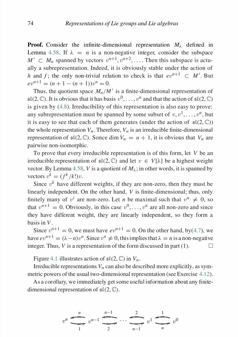
8/21/2019 Introduction to Lie Groups and Lie Algebras
http://slidepdf.com/reader/full/introduction-to-lie-groups-and-lie-algebras 86/236
74 Representations of Lie groups and Lie algebras
Proof. Consider the infinite-dimensional representation M λ defined in
Lemma 4.58. If λ
= n is a non-negative integer, consider the subspace
M ⊂ M n spanned by vectors vn+1, vn+2, . . . . Then this subspace is actu-
ally a subrepresentation. Indeed, it is obviously stable under the action of
h and f ; the only non-trivial relation to check is that evn+1 ⊂ M . But
evn+1 = (n + 1 − (n + 1))vn = 0.
Thus, the quotient space M n/ M is a finite-dimensional representation of
sl(2,C). It is obvious that it has basis v0, . . . , vn and that the action of sl(2,C)
is given by (4.8). Irreducibility of this representation is also easy to prove:
any subrepresentation must be spanned by some subset of v, v1, . . . , vn, but
it is easy to see that each of them generates (under the action of sl(2,C))
the whole representation V n. Therefore, V n is an irreducible finite-dimensional
representation of sl(2,C). Sonce dim V n = n + 1, it is obvious that V n are
pairwise non-isomorphic.
To prove that every irreducible representation is of this form, let V be an
irreducible representation of sl(2,C) and let v ∈ V [λ] be a highest weight
vector. By Lemma 4.58, V is a quotient of M λ; in other words, it is spanned by
vectors vk
= ( f k
/k !)v.Since v
k have different weights, if they are non-zero, then they must be
linearly independent. On the other hand, V is finite-dimensional; thus, only
finitely many of vi are non-zero. Let n be maximal such that vn = 0, so
that vn+1 = 0. Obviously, in this case v0, . . . , vn are all non-zero and since
they have different weight, they are linearly independent, so they form a
basis in V .
Since vn+1
= 0, we must have evn+1
= 0. On the other hand, by(4.7), we
have evn+1 = (λ−n)vn. Since vn = 0, this implies that λ = n is a non-negative
integer. Thus, V is a representation of the form discussed in part (1).
Figure 4.1 illustrates action of sl(2,C) in V n.
Irreducible representations V n can also be described more explicitly, as sym-
metric powers of the usual two-dimensional representation (see Exercise 4.12).
As a corollary, we immediately get some useful information about any finite-
dimensional representation of sl(2,C).
8/21/2019 Introduction to Lie Groups and Lie Algebras
http://slidepdf.com/reader/full/introduction-to-lie-groups-and-lie-algebras 87/236
4.9. Spherical Laplace operator and the hydrogen atom 75
Theorem 4.60. Let V be a finite-dimensional complex representation of
sl(2,C).
(1) V admits a weight decomposition with integer weights:
V =n∈Z
V [n].
(2) dim V [n] = dim V [−n]. Moreover, for n ≥ 0 the maps
en : V
[n
] → V
[−n
] f n : V [−n] → V [n]
are isomorphisms.
Proof. Since every representation is completely reducible, it suffices to prove
this in the case when V = V n is an irreducible representation. In this case, it
follows from Theorem 4.59.
By results of Section 4.1, this also implies similar statements for representa-tions of Lie algebra so(3,R) and the group SO(3,R). These results are given
in Exercise 4.13.
4.9. Spherical Laplace operator and the hydrogen atom
In this section, we apply our knowledge of representation theory of Lie groups
and Lie algebras to the study of the Laplace operator on the sphere, thus answer-
ing the question raised in the introduction. The material of this section will notbe used in the rest of the book, so it can be safely skipped. However, it is a
very illustrative example of how one uses representation theory in the study of
systems with a symmetry.
Let = ∂2 x + ∂2
y + ∂2 z be the usual Laplace operator in R3. We would like
to split it into “radial” and “spherical” parts, which can be done as follows.
Notice that R3 − {0} can be identified with the direct product
R3 − {0} S 2 × R+ ( )
8/21/2019 Introduction to Lie Groups and Lie Algebras
http://slidepdf.com/reader/full/introduction-to-lie-groups-and-lie-algebras 88/236
76 Representations of Lie groups and Lie algebras
Lemma 4.61.
(1) When rewritten in coordinates u, r, we have
= 1
r 2sph + radial,
where sph is a differential operator on S 2 and radial is a differential
operator on R+.
(2) We have
radial = ∂2r + 2r
∂r
sph = J 2 x + J 2 y + J 2 z ,
(4.10)
where
J x = y∂ z − z∂ y
J y = z∂ x − x ∂ z
J z = x ∂ y − y∂ x
are vector fields corresponding to the generators of Lie algebra so(3,R)
(see Exercise 3.11).
Sketch of proof. Since for any r > 0, the vector fields J x , J y, J z are tangent to
the sphere of radius r , the operator sph defined by (4.10) is well defined as a
differential operator on the sphere. Identity
= (1/r 2)sph
+radial can be
shown by explicit calculation (see Exercise 3.11).
One can introduce the usual coordinates on the sphere and write sph in these
coordinates. Such an expression can be found in any book on multivariable
calculus, but it is very messy; more importantly, it will be useless for our
purposes. For this reason it is not given here.
The main question we want to answer is as follows:
Find eigenvalues of sph acting on functions on S 2 (4.11)
8/21/2019 Introduction to Lie Groups and Lie Algebras
http://slidepdf.com/reader/full/introduction-to-lie-groups-and-lie-algebras 89/236
4.9. Spherical Laplace operator and the hydrogen atom 77
where ψ = ψ(t , x ), x ∈ R3, is the wave-function which describes the state of
the system and
H = − + V (r )
is the Hamiltonian, or the energy operator; here V (r ) is the potential, which
describes the central force field. Solving the Schrödinger equation is essentially
equivalent to diagonalizing the Hamiltonian. The usual approach to this problem
is to use separation of variables, writing
ψ( x ) = f i(r )gi(u) (4.12)
where r ∈ R+, u ∈ S 2 are given by (4.9), and gi are eigenfunctions for sph.
Substituting this in the equation H ψ = λψ gives a second-order differen-
tial equation on f i(r ). For many potentials V (r ), one can explicitly solve this
equation, thus giving eigenfunctions of the Hamiltonian – in particular, the
energy levels for the hydrogen atom. Details can be found, for example, in [34].
Returning to question (4.11), we notice that the straightforward approach,based on introducing coordinates on the sphere and writing the corresponding
partial differential equation, is rather complicated. Instead, we will use the
symmetries of the sphere, as was outlined in the introduction. We have an
obvious action of the group G = SO(3,R) on the sphere S 2 which therefore
defines an action of G on the space of functions on S 2, by g. f ( x ) = f (g−1( x )).
Lemma 4.62. sph : C ∞(S 2) → C ∞(S 2) commutes with the action of
SO(3,R
).
Proof. This can be shown in several ways. The easiest way is to note that it
is well known that the Laplace operator is rotation invariant. Obviously, the
radial part radial is also rotation invariant; thus, sph = r 2( −radial) is also
rotation invariant.
An alternative way of showing the rotational invariance of sph is by using
equality sph = J 2 x + J 2 y + J 2 z . Indeed, it suffices to show that in any represen-
tation V of SO(3,R
), the operator C = ρ( J x )
2
+ ρ( J y)
2
+ ρ( J z)
2
commuteswith the action of SO(3,R). By the results of Section 4.2, it is equivalent to
h ki h f h [ ( ) C] 0 Thi b il h
8/21/2019 Introduction to Lie Groups and Lie Algebras
http://slidepdf.com/reader/full/introduction-to-lie-groups-and-lie-algebras 90/236
78 Representations of Lie groups and Lie algebras
theory of Casimir elements, thus making the above computation unnecessary.
See Exercise 6.1 for details.
Therefore, by the general results of Section 4.4, the best way to study sph
would be to decompose the space of functions on S 2 into irreducible repre-
sentations of SO(3,R). As usual, it is more convenient to work with complex
representations, so we consider the space of complex-valued functions.
There are some obvious technical problems: the space of functions is infinite
dimensional. To avoid dealing with convergence questions and other analytical
difficulties, let us consider the space of polynomials
Pn =
Complex-valued functions on S 2 which can be written aspolynomials in x , y, z of total degree ≤ n
.
(4.13)
One easily sees that each Pn is a finite-dimensional representation of SO(3,R)
which is also sph-invariant. Thus, we can use the theory of finite-dimensional
representations to decompose Pn into irreducible representations and then usethis to find the eigenvalues of sph in Pn. Since
Pn = P is the space of
all polynomial functions on S 2, which is everywhere dense in C ∞(S 2), diago-
nalizing sph in P is essentially equivalent to diagonalizing sph in C ∞ (the
precise statement will be given below).
Thus, our immediate goal is to decompose Pn into a direct sum of irreducible
representations of SO(3,R). To do this, note that by results of Exercise 4.13,
irreducible representations of SO(3,R) are of the form V 2k , k
∈Z
+. Thus, we
can write
Pn =
ck V 2k .
To find coefficients ck , we need to find the character of Pn, i.e., the dimensions
of eigenspaces for J z (recall that under the isomorphism so(3,R)C sl(2,C)
constructed in Section 3.10, J z is identified with ih/2). We can do it by explicitly
constructing an eigenbasis in Pn.
Lemma 4.63. The following set of functions form a basis of Pn: |k| ik
8/21/2019 Introduction to Lie Groups and Lie Algebras
http://slidepdf.com/reader/full/introduction-to-lie-groups-and-lie-algebras 91/236
4.9. Spherical Laplace operator and the hydrogen atom 79
1 − z2 = x 2 + y2 = uv, every monomial zk ulv
m can be written as a monomial
which involves only u or v but not both. Thus, every element of Pn can be
written as a linear combination of monomials
z p,
z puk = z pρk eik ϕ = f p,k ,
z pv
k = z pρk e−ik ϕ = f p,−k
with p, k
∈Z
+, p
+k
≤ n. Thus, elements f p,k span Pn.
To show that they are linearly independent, assume thata p,k f p,k =
k
ak ( z)eik ϕ = 0, ak ( z) =
p
a p,k z p(
1 − z2|k |
.
By the uniqueness of Fourier series, we see that for every k ∈ Z, z ∈ (−1, 1),
we have ak ( z) = 0 which easily implies that for every p, k , a p,k = 0.
We can now find the dimensions of the eigenspaces for J z. Since J z is thegenerator of rotations around z axis, it is easy to see that in the cylindrical
coordinates z , ρ, ϕ, J z = ∂∂ϕ
. Thus,
J z f p,k = ikf p,k
so Pn[2k ] = Span( f p,k )0≤ p≤n−|k | and thus dim Pn[2k ] = n + 1 − k . Using the
formula for multiplicities from Exercise 4.11, we see that
Pn V 0 ⊕ V 2 ⊕ · · · ⊕ V 2n. (4.14)
Now the computation of the eigenvalues of spherical Laplace operator is easy.
Namely, by Exercise 4.4, J 2 x + J 2 y + J 2 z acts in V l by −l(l + 2)/4. Thus, we get
the following result.
Theorem 4.64. The eigenvalues of the spherical Laplace operator sph in the
space Pn areλk = −k (k + 1), k = 0, . . . , n (4.15)

8/21/2019 Introduction to Lie Groups and Lie Algebras
http://slidepdf.com/reader/full/introduction-to-lie-groups-and-lie-algebras 92/236
80 Representations of Lie groups and Lie algebras
Proof. Consider the space L2(S 2,C) of complex-valued L2 functions on S 2.
Since action of SO(3) preserves the volume form, it also preserves the inner
product in L2(S 2,C). It shows that operators J x , J y, J z are skew-Hermitian, and
thus, sph is Hermitian, or self-adjoint.
Let E n ⊂ Pn be the orthogonal complement to Pn−1. Then E n is SO(3)-
invariant, and it follows from (4.14) that as an SO(3)-module E n V 2n, so
sph acts on E n by λn. On the other hand, since the space of polynomials is
dense in L2, we have
L2(S 2,C)
=n≥0
E n
(direct sum of Hilbert spaces). Thus, if sph f = λ f for some function f ∈C ∞(S 2) ⊂ L2(S 2), then either λ = λn for all n, which forces ( f , E n) = 0 for
all n, so f = 0, or λ = λn, so ( f , E k ) = 0 for all k = n, so f ∈ E n.
4.10. Exercises
4.1. Let ϕ : SU(2) → SO(3,R) be the cover map constructed in
Exercise 2.8.
(1) Show that Ker ϕ = {1, −1} = {1, eπ ih}, where h is defined
by (3.23).
(2) Using this, show that representations of SO(3,R) are the same as
representations of sl(2,C) satisfying eπ iρ(h) = id.
4.2. Let V = C2
be the standard two-dimensional representation of the Liealgebra sl(2,C), and let S k V be the symmetric power of V .
(1) Write explicitly the action of e, f , h ∈ sl(2,C) (see Section 3.10) in
the basis ei1ek −i
2 .
(2) Show that S 2V is isomorphic to the adjoint representation
of sl(2,C).
(3) By results of Section 4.1, each representation of sl(2,C) can be con-
sidered as a representation of so(3,R). Which of representations S k V
can be lifted to a representation of SO(3,R)?
4 3 Sh h nCn C i f l( C) D i l k
8/21/2019 Introduction to Lie Groups and Lie Algebras
http://slidepdf.com/reader/full/introduction-to-lie-groups-and-lie-algebras 93/236
4.10. Exercises 81
(1) Show that C commutes with the action of sl(2,C): for any x ∈ sl(2,C), we have
[ρ( x ), C
] = 0. [Hint: use that for any a, b, c
∈End(V ), one has [a, bc] = [a, b]c + b[a, c].]
(2) Show that if V = V k is an irreducible representation with high-
est weight k , then C is a scalar operator: C = ck id. Compute the
constant ck .
(3) Recall that we have an isomorphism so(3,C) sl(2,C) (see
Section 3.10). Show that this isomorphism identifies operator C
above with a multiple of ρ ( J x )2 + ρ( J y)2 + ρ( J z)2.
The element C introduced here is a special case of more general notion
of Casimir element which will be discussed in Section 6.3.
4.5. (1) Let V , W be irreducible representations of a Lie group G. Show that
(V ⊗ W ∗)G = 0 if V is non-isomorphic to W , and that (V ⊗ V ∗)G
is canonically isomorphic to C.
(2) Let V be an irreducible representation of a Lie algebra g. Show
that V ∗ is also irreducible, and deduce from this that the space of
g-invariant bilinear forms on V is either zero or 1-dimensional.
4.6. For a representation V of a Lie algebrag, define the space of coinvaraints
by V g = V /gV , where gV is the subspace spanned by x v, x ∈ g, v ∈ V .
(1) Show that if V is completely reducible, then the composition V g →V → V g is an isomorphism.
(2) Show that in general, it is not so. (Hint: takeg = R and an appropriate
representation V .)
4.7. Let g be a Lie algebra, and ( , ) – a symmetric ad-invariant bilinear form
on g. Show that the element ω ∈ (g∗)⊗3 given by
ω( x , y, z) = ([ x , y], z)
is skew-symmetric and ad-invariant.
4.8. Prove that if A : Cn → Cn is an operator of finite order: Ak = I for
some k , then A is diagonalizable. [Hint: use theorem about complete
reducibility of representations of a finite group]
4 9 Let C be the standard cube in R3: C = {|x | ≤ 1} and let S be the set of
8/21/2019 Introduction to Lie Groups and Lie Algebras
http://slidepdf.com/reader/full/introduction-to-lie-groups-and-lie-algebras 94/236
82 Representations of Lie groups and Lie algebras
where the sum is taken over all faces σ which are neighbors of σ
(i.e., have a common edge with σ ). The goal of this problem is to
diagonalize A.
(1) Let G = {g ∈ O(3,R) | g(C ) = C } be the group of symmetries of
C . Show that A commutes with the natural action of G on V .
(2) Let z = − I ∈ G. Show that as a representation of G, V can be
decomposed in the direct sum
V = V + ⊕ V −, V ± = { f ∈ V | z f = ± f }.
(3) Show that as a representation of G, V + can be decomposed in the
direct sum
V + = V 0+ ⊕ V 1+, V 0+ = { f ∈ V + |
σ
f (σ ) = 0}, V 1+ = C · 1,
where 1 denotes the constant function on S whose value at every
σ
∈ S is 1.
(4) Find the eigenvalues of A on V −, V 0+, V 1+.
[Note: in fact, each of V −, V 0+, V 1+ is an irreducible representation of G ,
but you do not need this fact.]
4.10. Let G = SU(2). Recall that we have a diffeomorphism G S 3 (see
Example 2.5).
(1) Show that the left action of G on G S 3 ⊂ R4 can be extended to
an action of G by linear orthogonal transformations on R4.
(2) Let ω ∈ 3(G) be a left-invariant 3-form whose value at 1 ∈ G is
defined by
ω( x 1, x 2, x 3) = tr([ x 1, x 2] x 3), x i ∈ g
(see Exercise 4.7). Show that ω = ±4dV where dV is the volume
form on S 3 induced by the standard metric in R4 (hint: let x 1, x 2, x 3
be some orthonormal basis in su(2) with respect to 1
2
tr(a
¯bt )). (Sign
depends on the choice of orientation on S 3.)
(3) Sh th t
1
i bi i i t f G h th t f
8/21/2019 Introduction to Lie Groups and Lie Algebras
http://slidepdf.com/reader/full/introduction-to-lie-groups-and-lie-algebras 95/236
4.10. Exercises 83
4.12. Show that the symmetric power representation S k C2, considered in Exer-
cise 4.2, is isomorphic to the irreducible representation V k with highest
weight k .
4.13. Prove an analog of Theorem 4.60 for complex representations of so(3,R),
namely,
(1) Every finite-dimensional representation of so(3,R) admits a weight
decomposition:
V = n∈ZV [n],
where V [n] = {v ∈ V | J zv = in2 v}.
(2) A representation V of so(3,R) can be lifted to a representation of
SO(3,R) iff all weights are even: V [k ] = 0 for all odd k (cf. with
Exercise 4.1).
In physical literature, the number j = weight/2 is called the spin; thus,
instead of talking say, of representation with highest weight 3, physicicts
would talk about spin 3/2 representation. In this language, we see that arepresentation V of so(3,R) can be lifted to a representation of SO(3,R)
iff the spin is integer.
4.14. Complete the program sketched in Section 4.9 to find the eigenvalues
and multiplicities of the operator
H = − − c
r , c > 0
in L2(R3,C) (this operator describes the hydrogen atom).
8/21/2019 Introduction to Lie Groups and Lie Algebras
http://slidepdf.com/reader/full/introduction-to-lie-groups-and-lie-algebras 96/236
5
Structure theory of Lie algebras
In this section, we will start developing the structure theory of Lie algebras,
with the goal of getting eventually the full classification for semisimple Lie
algebras and their representations.
In this chapter, g will always stand for a finite-dimensional Lie algebra over
the ground field K which can be either R or C (most results will apply equally
in both cases and in fact for any field of characteristic zero). We will not beusing the theory of Lie groups.
5.1. Universal enveloping algebra
In a Lie algebra g, in general there is no multiplication: the products of the
form xy, x , y ∈ g, are not defined. However, if we consider a representation
ρ : g
→ gl(V ), then the product ρ( x )ρ( y) is well-defined in such a repre-
sentation – and in fact, as we will see later, operators of this kind can be
very useful in the study of representations. Moreover, the commutation rela-
tions in g imply some relations on the operators of this form. For example,
commutation relation [e, f ] = h in sl(2,C) implies that in any represen-
tation of sl(2,C) we have ρ(e)ρ( f ) − ρ( f )ρ (e) = ρ(h), or equivalently,
ρ(e)ρ( f ) = ρ(h) + ρ( f )ρ (e). These relations do not depend on the choice of
representation ρ .
Motivated by this, we define the “universal” associative algebra generatedby products of operators of the form ρ ( x ), x ∈ g.
8/21/2019 Introduction to Lie Groups and Lie Algebras
http://slidepdf.com/reader/full/introduction-to-lie-groups-and-lie-algebras 97/236
5.1. Universal enveloping algebra 85
To simplify the notation, we (and everyone else) will usually write simply
x
∈ U g instead of i( x ). This will be justified later (see Corollary 5.13) when
we show that the map i : g → U g is injective and thus g can be considered as
a subspace in U g.
If we dropped relation (5.1), we would get the associative algebra generated
by elements x ∈ g with no relations other than linearity and associativity. By
definition, this is exactly the tensor algebra of g:
T g =
n≥0
g⊗n. (5.2)
Thus, one can alternatively describe the universal enveloping algebra as the
quotient of the tensor algebra:
U g = T g/( xy − yx − [ x , y]), x , y ∈ g. (5.3)
Example 5.2. Let g be a commutative Lie algebra. Then U g is generated by
elements x ∈ g with relations xy = yx . In other words, U g = S g is the
symmetric alebra of g, which can also be described as the algebra of polynomialfunctions on g∗. Choosing a basis x i in g we see that U g = S g = K[ x 1, . . . , x n].
Note that in this example, the universal enveloping algebra is infinite-
dimensional. In fact, U g is always infinite-dimensional (unless g = 0). We
will return to the discussion of the size of U g in the next section.
Example 5.3. The universal enveloping algebra of sl(2,C) is the associative
algebra over C generated by elements e, f , h with the relations ef − ef = h,
he − eh = 2e, hf − fh = −2 f .
It should be noted that even when g ⊂ gl(n,K) is a matrix algebra, multipli-
cation in U g is different from multiplication of matrices. For example, let e be
the standard generator of sl(2,C). Then e2 = 0 as a 2 × 2 matrix, but e2 = 0
in U g – and for a good reason: there are many representations of sl(2,C) in
which ρ (e)2 = 0.
The following theorem shows that U g is indeed universal in a certain sense,
which justifies the name.
Theorem 5.4. Let A be an associative algebra with unit over K and let
8/21/2019 Introduction to Lie Groups and Lie Algebras
http://slidepdf.com/reader/full/introduction-to-lie-groups-and-lie-algebras 98/236
86 Structure theory of Lie algebras
In other words, categories of representations of g and of U g-modules are
equivalent.
As a useful application of this result, we can use U g to construct various
operators acting in representations of g – in particular to construct intertwining
operators.
Example 5.6. Let C = ef + fe + 12
h2 ∈ U sl(2,C). Then
eC = e2 f + efe + 1
2eh2 = e( fe + h) + ( fe + h)e + 1
2(he − 2e)h
= efe + fe2 + 1
2heh + eh + he − eh = efe + fe2 1
2h(he − 2e) + he
= efe + fe2 1
2h2e = Ce.
The idea of this calculation is to move e to the right, using the relations ef = fe + h, eh = he − 2e to interchange it with f , h. Similar calculations also show
that fC
= Cf , hC
= Ch. Thus, C is central in U g.
In particular, this implies that in every representation V of sl(2,C), the ele-
ment ρ(C ) : V → V commutes with the action of sl(2,C) and thus is an
intertwining operator. By Schur lemma (Lemma 4.23), this shows that C acts
by a constant in every irreducible representation. And if V is not irreducible,
eigenspaces of V are subrepresentations, which could be used to decompose V
into irreducible representations (see Lemma 4.21).
Element C is called the Casimir operator for sl(2,C). We will discuss its
generalization for other Lie algebras in Proposition 6.15.
Proposition 5.7.
(1) The adjoint action of g on g can be uniquely extended to an action of g
on U g which satisfies Leibniz rule: ad x .(ab) = (ad x .a)b + a(ad x .b), x ∈g, a, b ∈ U g. Moreover, ad x .a = xa − ax.
(2) Let Z g = Z (U g) be the center of universal enveloping algebra. Then Z g
coincides with the space of invariants of U g with respect to the adjoint
action of g:
8/21/2019 Introduction to Lie Groups and Lie Algebras
http://slidepdf.com/reader/full/introduction-to-lie-groups-and-lie-algebras 99/236
5.2. Poincare–Birkhoff–Witt theorem 87
ad x (ad y.a) − ad y(ad x .a), or
[ x , y]a − a[ x , y] = x ( ya − ay) − ( ya − ay) x − ( y( xa − ax )
−( xa − ax ) y) ,
which is given by explicit calculation.
Leibniz rule follows from
xab − abx = ( xa − ax )b + a( xb − bx ).
This proves the first part. The second part follows immediately: C ∈ U g iscentral iff it commutes with all the generators, i.e. if Cx = xC for any x ∈ g.
The last condition is equivalent to ad x .C = 0.
5.2. Poincare–Birkhoff–Witt theorem
In this section, g is a finite-dimensional Lie algebra over the field K and U g is
the universal enveloping algebra of g.
We had already mentioned that U g is infinite-dimensional. In this section,we will give a more precise statement.
Unlike polynomial algebra, U g is not graded: if we try to define degree by
deg( x 1 . . . x k ) = k , x i ∈ g, then we run into problem with the defining relation
(5.1): we would have deg( xy)= deg( yx )=2, but deg( xy − yx )= deg([ x , y])=1.
Instead, we have a weaker structure: we can define filtration on U g by letting,
for any k ≥ 0,
U k g = Subspace in U g spanned by products x 1 . . . x p, p ≤ k . (5.4)
This defines a filtration on U g: we have
K = U 0g ⊂ U 1g ⊂ . . . , U g =
U pg.
The following proposition gives some properties of this filtration.
Proposition 5.8.
(1) U g is a filtered algebra: if x ∈ U pg, y ∈ U qg , then xy ∈ U p+qg.
(2) If x ∈ U g y ∈ U g then xy yx ∈ U 1g
8/21/2019 Introduction to Lie Groups and Lie Algebras
http://slidepdf.com/reader/full/introduction-to-lie-groups-and-lie-algebras 100/236
88 Structure theory of Lie algebras
Proof. Part (1) is obvious. To prove the second part, note that for p = 1, we
have
x ( y1 . . . yq) − ( y1 . . . yq) x =
i
y1 . . . [ x , yi] . . . yq ∈ U qg.
In particular, this implies that for any x ∈ g, y ∈ U qg, we have xy ≡ yx
mod U qg.
Now we can argue by induction in p: if the statement is true for some p, then
x 1 . . . x p+1 y ≡ x 1 . . . x p yx p+1 ≡ yx 1 . . . x p x p+1 mod U p+q−1g.
Part (3) is again proved by induction in p. Indeed, for p = 1 it is obvious. To
establish the induction step, notice that U p+1g is generated by elements of the
form xy, x ∈ g, y ∈ U pg. By induction assumption, y can be written as linear
combination of monomials of the form (5.5). But by part (2),
x i( x k 11 . . . x k n
n )
− x
k 11 . . . x
k i+1i . . . x k n
n
∈ U pg.
Using the induction assumption again, we see that x i( x k 11 . . . x
k nn ) can again be
written as linear combination of monomials of the form (5.5), with
k i ≤ p + 1.
Corollary 5.9. Each U pg is finite-dimensional.
Corollary 5.10. The associated graded algebra
Gr U g = p
U pg/U p−1g (5.6)
is commutative.
We can now formulate the main result of this section.
Theorem 5.11 (Poincaré–Birkhoff–Witt). Let x 1, . . . , x n be an ordered basis
is g. Then monomials of the form (5.5) form a basis in U pg.
Th f f hi h i i h i b f d f l
8/21/2019 Introduction to Lie Groups and Lie Algebras
http://slidepdf.com/reader/full/introduction-to-lie-groups-and-lie-algebras 101/236
5.2. Poincare–Birkhoff–Witt theorem 89
Namely, we consider (infinite-dimensional) vector space V with basis given
by (5.5) (no restriction on k i). The action is uniquely defined by the require-
ment that ρ( x i). x j1 . . . x jn = x i x j1 . . . x jn if i ≤ j1 ≤ j2 . . . . For example, this
forces ρ ( x 1). x 2 = x 1 x 2.
This requirement also determines ρ( x i). x j1 . . . x jn if i > j1. For example, to
define ρ( x 2). x 1, we note that it must be equal to ρ( x 2)ρ( x 1).1 = ρ ( x 1)ρ( x 2).1+ρ([ x 2, x 1]).1 = x 1 x 2 +
ai x i, where ai are defined by [ x 1, x 2] =
ai x i.
The difficult part is to check that it is indeed an action, i.e., that it satisfies
ρ( x )ρ( y) − ρ( y)ρ( x ) = ρ [ x , y], which is done by an explicit calculation using
the Jacobi identity.
Note that this theorem would fail without the Jacobi identity: if [ , ] : g ⊗g → g is an antisymmetric map not satisfying Jacobi identity, then the algebra
defined by (5.1) can be trivial (i.e., all i( x ) = 0).
This theorem can also be reformulated in a coordinate-independent way.
Theorem 5.12 (Poincaré–Birkhoff–Witt). The graded algebra Gr U g defined
by (5.6) is naturally isomorphic to the symmetric algebra S g. The isomorphism
is given by
S pg → Gr p U g
a1 . . . a p → a1 . . . a p mod U p−1g(5.7)
and the inverse isomorphism is given by
Gr p U g → S pg
a1 . . . a p → a1 . . . a p,
a1 . . . al → 0, l < p.
(5.8)
When written in this form, this theorem may seem trivial. The non-triviality
is hidden in the statement that the maps (5.7), (5.8) are well-defined.
The Poincaré–Birkhoff–Witt (or PBW for short) theorem has a number of
useful corollaries. Here are some of them; proofs are left as an easy exercise to
the reader.
Corollary 5.13. The natural map g
→ U g is injective.
Corollary 5.14. Let g1, g2 ⊂ g be subalgebras such that g = g1 ⊕ g2 as a
( d i h ) Th h l i li i

8/21/2019 Introduction to Lie Groups and Lie Algebras
http://slidepdf.com/reader/full/introduction-to-lie-groups-and-lie-algebras 102/236
90 Structure theory of Lie algebras
Corollary 5.15. Algebra U g has no zero divisors.
Notice that while Theorem 5.12 establishes an isomorphism between Gr U gand S g, this isomorphism clearly can not be extended to an isomorphism of
algebras U g ∼−→ S g unless g is commutative. The following result, the proof of
which is left as an exercise for the reader, is the best one can get in this direction
for general g.
Theorem 5.16. The map S g → U g given by
sym( x 1 . . . x p) = 1
p! s∈S p
x s(1) . . . x s( p) (5.9)
is an isomorphism of g-modules.
This isomorphism will be later used in the construction of so-called Harish–
Chandra isomorphism (see Section 8.8).
5.3. Ideals and commutant
Recall that a subalgebra of g is a vector subspace closed under the commutator,
and an ideal is a vector subspace h such that [ x , y] ∈ h for any x ∈ g, y ∈ h. This
definition is the natural analog of an ideal in an associative algebra. Note, how-
ever, that because of skew-symmetry of the commutator there is no difference
between left and right ideals: every right ideal is also automatically a left ideal.
As in the theory of associative algebras, if h is an ideal of g then the quotientspace g/h has a canonical structure of a Lie algebra, and we have the following
trivial result, proof of which is left to the reader as an exercise.
Lemma 5.17. If f : g1 → g2 is a morphism of Lie algebras, then Ker f is an
ideal in g1, Im f is a subalgebra in g2 , and f gives rise to an isomorphism of
Lie algebras g/ Ker f Im f .
In addition, here is another important result about ideals, proof of which is
left as an easy exercise to the reader.
Lemma 5 18 Let I I be ideals in g Define
8/21/2019 Introduction to Lie Groups and Lie Algebras
http://slidepdf.com/reader/full/introduction-to-lie-groups-and-lie-algebras 103/236
5.4. Solvable and nilpotent Lie algebras 91
One of the first ways to study Lie algebras is by analyzing how close the Lie
algebra is to a commutative Lie algebra. There are several ways of making it
precise.
First, we might look at how large the center z(g) = { x ∈ g | [ x , y] = 0 for all
y ∈ g} is. However, it turns out that it is more effective to study commutative
quotients of g.
Definition 5.19. The commutant of a Lie algebra g is the ideal [g, g].
The following lemma explains the importance of the commutant.
Lemma 5.20. The quotient g/[g, g] is an abelian Lie algebra. Moreover, [g, g]is the smallest ideal with this property: if g/ I is abelian for some ideal I ⊂ g ,
then I ⊃ [g, g].
Commutant gives us another way of measuring how far a Lie algebra
is from being commutative: the smaller [g, g] (and the larger g/[g, g]), the
closer g is to being commutative. For example, for commutative g, we have
[g, g
] = 0.
Example 5.21. The commutant [gl(n,K), gl(n,K)] = [ sl(n,K), sl(n,K)] = sl(n,K). Indeed, it is obvious that for any z = [ x , y] we have tr z = 0. On the
other hand, for i = j we have E ii − E jj = [ E ij, E ji] and 2 E ij = [ E ii − E jj, E ij],
which shows that E ii − E jj, E ij ∈ [ sl(n,K), sl(n,K)]. Since these elements span
sl(n,K) we see that [gl(n,K), gl(n,K)] = [ sl(n,K), sl(n,K)] = sl(n,K).
5.4. Solvable and nilpotent Lie algebras
We now can define an important class of Lie algebras.
Definition 5.22. For a Lie algebra g, define the series of ideals Dig (called the
derived series) by D0g = g and
Di+1g = [ Dig, Dig].
It immediately follows from Lemmas 5.18 and 5.20 that each Di is an ideal
i d Di /Di+1 i b li
8/21/2019 Introduction to Lie Groups and Lie Algebras
http://slidepdf.com/reader/full/introduction-to-lie-groups-and-lie-algebras 104/236
92 Structure theory of Lie algebras
(3) For large enough n, every commutator of the form
[. . . [[ x 1, x 2], [ x 3, x 4]] . . . ]
(2n terms, arranged in a binary tree of length n) is zero.
Proof. Equivalence of (1) and (3) is obvious. Implication (1) =⇒ (2) is also
clear: we can take a i = Dig. To prove (2) =⇒ (1), note that if a i satisfies the
conditions of the proposition, then by Lemma 5.20, we have ai+1 ⊃ [ai, ai].
Thus, reasoning by induction, we see that ai
⊃ Dig.
Definition 5.24. Lie algebra g is called solvable if it satisfies any of the
equivalent conditions of Proposition 5.23.
Informally, a solvable Lie algebra is an “almost commutative” Lie algebra:
it is an algebra that can be obtained by successive extensions of commutative
algebras.
This is not the only way of making the notion of “almost commutative” Lie
algebra precise. Another class of Lie algebras can be defined as follows.
Definition 5.25. For a Lie algebra g, define a series of ideals Dig ⊂ g (called
lower central series) by D0g = g and
Di+1g = [g, Dig].
Proposition 5.26. The following conditions are equivalent:
(1) Dng = 0 for large enough n.
(2) There exists a sequence of ideals a0 = g ⊃ a1 ⊃ · · · ⊃ ak = {0} such that
[g, ai] ⊂ ai+1.
(3) For large enough n, every commutator of the form
[. . . [[ x 1, x 2], x 3], x 4] . . . x n]
(n terms) is zero.
8/21/2019 Introduction to Lie Groups and Lie Algebras
http://slidepdf.com/reader/full/introduction-to-lie-groups-and-lie-algebras 105/236
5.4. Solvable and nilpotent Lie algebras 93
Example 5.28. Let b ⊂ gl(n,K) be the subalgebra of upper triangular matrices,
and n be the subalgebra of all strictly upper triangular matrices. Then b is
solvable, and n is nilpotent.
To prove it, let us first generalize it. Namely, if F is a flag in a finite-
dimensional vector space V :
F = ({0} ⊂ V 1 ⊂ V 2 ⊂ . . . V n = V )
with dim V i < dim V i+1 (we do not require that dim V i = i), then define
b(F ) = { x ∈ gl(V ) | xV i ⊂ V i for all i},
n(F ) = { x ∈ gl(V ) | xV i ⊂ V i−1 for all i}.
By taking F to be the standard flag in Kn (see Example 2.25) we recover the
Lie algebras b, n defined above.
We claim that n(F ) is nilpotent. Indeed, define more general algebras
ak (F ) = { x ∈ gl(V ) | xV i ⊂ V i−k for all i}
so that b(F ) = a0, n(F ) = a1. Then it is obvious that for x ∈ ak , y ∈ al , we
have xy ∈ ak +l (here xy is the usual product in End(V )); thus, [ak , al] ⊂ ak +l ,
so Din ⊂ ai+1. This proves nilpotency of n(F ).
To show solvability of b (for the standard flag F ), note that even though for
x , y ∈ b we can only say that xy ∈ b, for the commutator we have a stronger
condition:
[ x , y
] ∈ n
= a1. Indeed, diagonal entries of xy and yx coincide. Thus,
D1b ⊂ n = a1. From here it easily follows by induction that Di+1b ⊂ a2i .
Note, finally, that b is not nilpotent: D2b = [b, D1b] = D1b = n, which can
be easily deduced from [ x , E ij] = (λi − λ j) E ij if x is a diagonal matrix with
entries λi.
The following theorem summarizes some basic properties of solvable and
nilpotent Lie algebras.
Theorem 5.29.
(1) A real Lie algebra g is solvable (respectively nilpotent) iff its complexifi
8/21/2019 Introduction to Lie Groups and Lie Algebras
http://slidepdf.com/reader/full/introduction-to-lie-groups-and-lie-algebras 106/236
94 Structure theory of Lie algebras
Proof. Parts (1), (2) are obvious if we use definition of solvable algebra in
the form “any commutator of the form … is zero”, and similarly for nilpotent.
Part (3) follows from inclusion Dig ⊂ Dig, which can be easily proved by
induction.
Finally, to prove part (4), denote by ϕ the canonical projection g → g/ I .Then
ϕ( Dng) = Dn(g/ I ) = 0 for some n. Thus, Dng ⊂ I . Therefore, Dn+k g ⊂ Dk I ,
so Dn+k g = 0 for large enough k .
5.5. Lie’s and Engel’s theorems
The main result of this section is the following theorem.
Theorem 5.30 (Lie’s theorem about representations of a solvable Lie algebra).
Let ρ : g → gl(V ) be a complex representation of a solvable Lie algebra g (real
or complex ). Then there exists a basis in V such that in this basis, all operators
ρ( x ) are upper-triangular.
This theorem is a generalization of a well-known result that any operator in
a complex vector space can be brought to an upper-triangular form by a change
of basis.
The key step in the proof of the theorem is the following result.
Proposition 5.31. Let ρ : g → gl(V ) be a complex representation of a solvable
Lie algebra g. Then there exists a vector v ∈ V which is a common eigenvector
of all ρ ( x ), x ∈ g.
Proof. The proof goes by induction in dimension of g. Since g is solvable,
[g, g] = g. Let g ⊂ g be a subspace which contains [g, g] and has codimension1 in g:g = g ⊕ C x . Then g is an ideal in g; thus, g is solvable.
By induction assumption, there exists v ∈ V which is a common eigenvector
for all ρ(h), h ∈ g:ρ(h)v = λ(h)v. Consider the vector space W spanned by
v0 = v, v1 = ρ( x )v, v2 = (ρ( x ))2
v, . . . .
We claim that W is stable under the action of any h ∈ g; moreover,
hvk = λ(h)vk +l<k
akl (h)vl . (5.10)
This is easily proved by induction: indeed
8/21/2019 Introduction to Lie Groups and Lie Algebras
http://slidepdf.com/reader/full/introduction-to-lie-groups-and-lie-algebras 107/236
5.5. Lie’s and Engel’s theorems 95
Let n be the smallest integer such that vn+1 is in the subspace generated by
v0, v1, . . . , vn. Then v
0, v1, . . . , vn is a basis in W . By (5.10), in this basis any
ρ(h) is upper-triangular, with λ(h) on the diagonal. In particular, this implies
that trW ρ(h) = (n + 1)λ(h).
Since trW [ρ( x ), ρ(h)] = 0, this implies that λ([h, x ]) = 0 for any h ∈ g. The
same calculation as in (5.11), shows that this implies hvk = λ(h)vk . Therefore,
any vector w ∈ W is a common eigenvector for all h ∈ g. Choosing w to be
an eigenvector for x , we get the statement of the proposition.
This proposition immediately implies Lie’s theorem.
Proof of Theorem 5.30. Proof goes by induction in dim V . By Proposi-
tion 5.31, there exists a common eigenvector v for all x ∈ g. Consider the
space V /Cv. By induction assumption, there exists a basis v1, v2, . . . in V /Cv
such that the action of g in this basis of V /Cv is upper-triangular. For each of
these vectors, choose a preimage vi ∈ V . Then one immediately sees that the
action of any x ∈ g in the basis v, v1, v2, . . . is upper-triangular.
This theorem gives a number of useful corollaries.
Corollary 5.32.
(1) Any irreducible complex representation of a solvable Lie algebra is one-
dimensional.
(2) If a complex Lie algebra g is solvable, then there exists a sequence 0 ⊂ I 1 ⊂
· · · ⊂ I
n = g , where each I
k is an ideal in g and I
k +1/ I
k is one-dimensional.
(3) g is solvable if and only if [g, g] is nilpotent.
Proof. Part (1) is obvious from Proposition 5.31; part (2) is immediately
obtained if we apply Lie’s theorem to the adjoint representation and note that a
subrepresentation of the adjoint representation is the same as an ideal in g.
To prove part (3), note that implication in one direction is obvious. Indeed,
if [g, g] is nilpotent, then it is also solvable; since g/[g, g] is commutative (and
thus solvable), by Theorem 5.29, g itself is solvable.Conversely, assume that g is solvable. Without loss of generality, we may
h i l A l Li ’ h h dj i i B
8/21/2019 Introduction to Lie Groups and Lie Algebras
http://slidepdf.com/reader/full/introduction-to-lie-groups-and-lie-algebras 108/236
96 Structure theory of Lie algebras
One also might ask if there is an analog of Lie’s theorem for nilpotent Lie
algebras. Of course, since every nilpotent Lie algebra is automatically solvable
(Theorem 5.29), Lie’s theorem shows that in any representation of a nilpotent
algebra, operators ρ( x ) are upper-triangular in a certain basis. One wonders
whether one has a stronger result – for example, whether operators ρ ( x ) can be
made strictly upper-triangular. Here the answer is obviously negative: it suffices
to take a commutative Lie algebra which acts diagonally in Cn.
The proper analog of Lie’s theorem for nilpotent Lie algebras is given by the
following result.
Theorem 5.33. Let V be a finite-dimensional vector space, either real or com- plex, and let g ⊂ gl(V ) be a Lie subalgebra which consists of nilpotent
operators. Then there exists a basis in V such that all operators x ∈ g are
strictly upper-triangular.
The proof of this theorem will not be given here; interested reader can find
it in [46], [24], or [22]. It is not very difficult and in fact is rather similar to the
proof of Lie’s theorem; the only reason it is not given here is because it does
not give any new insight.As an immediate corollary, we get the following theorem.
Theorem 5.34 (Engel’s theorem). A Lie algebra g is nilpotent if and only if for
every x ∈ g , the operator ad x ∈ End(g) is nilpotent.
Proof. One direction is obvious: if g is nilpotent then by definition,
[ x , [ x , . . . [ x , y . . . ] = (ad x )n. y = 0 for large enough n.
Conversely, if ad x is nilpotent for every x , then by the previous theorem,
there exists a sequence of subspaces 0 ⊂ g1 ⊂ g2 · · · ⊂ gn = g such that
ad x .gi ⊂ gi−1. This shows that each gi is an ideal in g and moreover, [g, gi] ⊂gi−1. Thus, g is nilpotent.
5.6. The radical. Semisimple and reductive algebras
So far, we have defined the notion of a solvable Lie algebra; informally,
a solvable Lie algebra is the one which is close to being abelian. In this
section, we will describe the opposite extreme case, Lie algebras which are
8/21/2019 Introduction to Lie Groups and Lie Algebras
http://slidepdf.com/reader/full/introduction-to-lie-groups-and-lie-algebras 109/236
5.6. The radical. Semisimple and reductive algebras 97
Note that this in particular implies that the center z(g) = 0.
A special case of semisimple Lie algebras is given by simple ones.
Definition 5.36. A Lie algebra g is called simple if it is not abelian and contains
no ideals other than 0 and g.
The condition that g should not be abelian is included to rule out the one-
dimensional Lie algebra: there are many reasons not to include it in the class
of simple Lie algebras. One of these reasons is the following lemma.
Lemma 5.37. Any simple Lie algebra is semisimple.
Proof. If g is simple, then it contains no ideals other than 0 and g. Thus, if g
contains a nonzero solvable ideal, then it must coincide with g, so g must be
solvable. But then [g, g] is an ideal which is strictly smaller than g (because g is
solvable) and nonzero (because g is not abelian). This gives a contradiction.
Example 5.38. The Lie algebra sl(2,C) is simple. Indeed, recall that ad h is
diagonal in the basis e, f , h, with eigenvalues 2, −2, 0 (see Section 3.10). Any
ideal in g must be stable under ad h. Now we can use the following easy to
prove result from linear algebra: if A is a diagonalizable operator in a finite-
dimensional vector space, with distinct eigenvalues: Avi = λivi, λi = λ j , then
the only subspaces invariant under A are those spanned by some of the eigen-
vectors vi. Applying this to ad h, we see that any ideal in sl(2,C) must be
spanned as a vector space by a subset of {e, f , h}.
But if an ideal I contains h, then [h, e] = 2e ∈ I , [h, f ] = −2 f ∈ I , so
I = sl(2,C). If I contains e, then [e, f ] = h ∈ I , so again I = sl(2,C).
Similarly, if f ∈ I , then I = sl(2,C). Thus, sl(2,C) contains no non-trivialideals.
In the next section, we will generalize this result and show that classical Lie
algebras such as sl(n,C), su(n), sp(n,C), so(n,C) are semisimple.
For a general Lie algebra g, which is neither semisimple nor solvable, we
can try to “separate” the solvable and semisimple parts.
Proposition 5.39. In any Lie algebra g , there is a unique solvable ideal which
contains any other solvable ideal. This solvable ideal is called the radical of gand denoted by rad(g).

8/21/2019 Introduction to Lie Groups and Lie Algebras
http://slidepdf.com/reader/full/introduction-to-lie-groups-and-lie-algebras 110/236
98 Structure theory of Lie algebras
the sum is taken over all solvable ideals (finite-dimensionality of g shows that
it suffices to take a finite sum).
Using this definition, we can rewrite the definition of a semisimple Lie algebra
as follows: g is semisimple iff rad(g) = 0.
Theorem 5.40. For any Lie algebra g , the quotient g/ rad(g) is semisimple.
Conversely, if b is a solvable ideal in g such that g/b is semisimple, then
b = rad(g).
Proof. Assume that g/ rad(g) contains a solvable ideal I . Consider the ideal
˜ I = π−1( I ) ⊂ g, where π is the canonical map g → g/ rad(g). Then ˜ I ⊃rad(g) and ˜ I / rad(g) = I is solvable. Thus, by Theorem 5.29, ˜ I is solvable, so˜ I = rad(g), I = 0.
Proof of the second statement is left to the reader as an exercise.
This theorem shows that any Lie algebra can be included in a short exact
sequence 0 → b → g → gss → 0, where b is solvable and gss is semisimple.
In fact, one has a much stronger result.
Theorem 5.41 (Levi theorem). Any Lie algebra can be written as a direct sum
g = rad(g) ⊕ gss, (5.12)
where gss is a semisimple subalgebra (not necessarily an ideal!) in g. Such a
decomposition is called the Levi decomposition for g.
This theorem will not be proved here. A proof can be found in standard
textbooks on Lie algebras, such as [46] or [24]. We only mention here that thekey step in the proof is showing vanishing of a certain cohomology group; we
will say more about this in Section 6.3.
Example 5.42. Let G = SO(3,R) R3 be the Poincare group, i.e. the group
of all mapsR3 → R3 which have the form x → Ax +b, A ∈ SO(3,R), b ∈ R3.
The corresponding Lie algebra is g = so(3,R) ⊕R3, where the commutator is
given by
[( A1, b1), ( A2, b2)
] = (
[ A1, A2
], A1b2
− A2b1). Thus,R3 is an ideal and
so(3,R) is a subalgebra. Since R3 is abelian and so(3,R) is semisimple (whichfollows from semisimplicity of so(3,R)C sl(2,C), see Example 5.38), we
8/21/2019 Introduction to Lie Groups and Lie Algebras
http://slidepdf.com/reader/full/introduction-to-lie-groups-and-lie-algebras 111/236
5.7. Invariant bilinear forms and semisimplicity 99
Theorem 5.43. Let V be an irreducible complex representation of g. Then
any h
∈ rad(g) acts in V by scalar operators: ρ(h)
= λ(h) id. Also, any
h ∈ [g,rad(g)] acts by zero.
Proof. By Proposition 5.31, there is a common eigenvector in V for all
h ∈ rad(g):ρ(h).v = λ(h)v for some λ : rad(g) → C. Define V λ = {w ∈V | ρ(h)w = λ(h)w for all h ∈ rad(g)}. Then the same argument as in the
proof of Proposition 5.31 shows that for any x ∈ g, one has ρ( x )(V λ) ⊂ V λ.
Thus, V λ is a subrepresentation; since it is non-zero and V is irreducible, we
must have V = V λ, which proves the first statement of the theorem. The second
statement immediately follows from the first one.
From the point of view of representation theory, having non-zero elements
which act by zero in any irreducible representation significantly compli-
cates the theory. Thus, it is natural to consider a class of algebras for which
[g,rad(g)] = 0.
Definition 5.44. ALie algebra is called reductive if rad(g) = z(g), i.e. if g/ z(g)
is semisimple. (Recall that z(g) is the center of g.)
Of course, any semisimple Lie algebra is reductive (because then rad(g) = z(g) = 0), but the converse is not true: for example, any Lie algebra which is
a direct sum of an abelian and semisimple algebras
g = z ⊕ gss, [ z, gss] = 0, (5.13)
is reductive. In fact, it follows from the Levi theorem that any reductive Lie
algebra must have such form. Later we will give an alternative proof of thisresult, which does not use the Levi theorem (see Theorem 6.24).
In the next section we will show that many classical Lie algebras such as
gl(n,C) or u(n) are reductive.
5.7. Invariant bilinear forms and semisimplicity
of classical Lie algebras
So far, we have only one example of a semisimple Lie algebra, namely sl(2,C)
(see Example 5.38), and the proof of its semisimplicity was done by brute force,
b l i ll ibiliti f id l It i l th t h f ld b

8/21/2019 Introduction to Lie Groups and Lie Algebras
http://slidepdf.com/reader/full/introduction-to-lie-groups-and-lie-algebras 112/236
100 Structure theory of Lie algebras
for any x , y, z ∈ g (see Example 4.15). The following lemma shows the
importance of such forms.
Lemma 5.45. Let B be an invariant bilinear form on g , and I ⊂ g an ideal. Let
I ⊥ be the orthogonal complement of I with respect to B: I ⊥={ x ∈ g | B( x , y)=0
for all y ∈ I }. Then I ⊥ is also an ideal in g. In particular, Ker B = g⊥ is an
ideal in g.
The proof of this lemma is trivial and left to the reader. Note, however, that
in general we can not write g = I ⊕ I ⊥, as it is quite possible that I ∩ I ⊥ = 0,
even for a non-degenerate form B.
Example 5.46. Let g = gl(n,C) and define the form by B( x , y) = tr( xy). Then
it is a symmetric invariant bilinear form on g. Indeed, symmetry is well-known
and invariance follows from the following identity
tr([ x , y] z + y[ x , z]) = tr( xyz − yxz + yxz − yzx ) = tr( xyz − yzx ) = 0.
In fact, there is an even easier proof: since tr (gxg−
1gyg−
1) =
tr(gxyg−
1) =tr( xy) for any g ∈ GL(n,C), we see that this form is invariant under the adjoint
action of GL(n,C) which is equivalent to the invariance under the action of
gl(n,C).
This example can be easily generalized.
Proposition 5.47. Let V be a representation of g and define a bilinear form on
g by
BV ( x , y) = trV (ρ( x )ρ( y)). (5.14)
Then BV is a symmetric invariant bilinear form on g.
The proof is identical to the proof in Example 5.46.
However, this form can be degenerate or even zero. It turns out, how-
ever, that there is a close relation between non-degeneracy of such forms and
semisimplicity of g.
Theorem 5.48. Let g be a Lie algebra with a representation V such that the form BV defined by (5.14) is non-degenerate. Then g is reductive.
8/21/2019 Introduction to Lie Groups and Lie Algebras
http://slidepdf.com/reader/full/introduction-to-lie-groups-and-lie-algebras 113/236
5.8. Killing form and Cartan’s criterion 101
we would have x ∈ Ker BV . Since by assumption BV is non-degenerate,
this shows x
= 0.
As an immediate corollary, we have the following important result.
Theorem 5.49. All classical Lie algebras of Section 2.7 are reductive. Algebras
sl(n,K), so(n,K) (n > 2), su(n), sp(n,K) are semisimple; algebras gl(n,K)
and u(n) have one-dimensional center: gl(n,K) = K · id ⊕ sl(n,K) , u(n) =iR · id ⊕ su(n). ( As before, K is either R or C.)
Proof. For each of these subalgebras, consider the trace form BV where V is the
defining representation (Kn for gl(n,K), sl(n,K), so(n,K);Cn for su(n), u(n)
andK2n for sp(n,K)). Then this form is non-degenerate. Indeed, for gl(n) it fol-
lows because B( x , y) = x ij y ji, which is obviously non-degenerate; for sl(n)
it follows from the result for gl(n) and decomposition gl(n) = K · id ⊕ sl(n),
with the two summands being orthogonal with respect to the form B.
For so(n), we have B( x , y) = x ij y ji = −2
i> j x ij yij so it is again non-
degenerate. Similarly, for u(n) we have B( x , y) = − tr xyt = −
x ij yij; in
particular, B( x , x ) = − | x ij|2
, so this form is negative definite and in partic-ular, non-degenerate. Therefore, its restriction to su(n) ⊂ u(n) is also negative
definite and thus non-degenerate.
The non-degeneracy of this form for sp(n,K) is left as an exercise
(Exercise 5.4).
Thus, by Theorem 5.48 we see that each of these Lie algebras is reductive.
Since the center of each of them is easy to compute (see Example 4.24), we get
the statement of the theorem.
5.8. Killing form and Cartan’s criterion
In the previous section, we have shown that for any representation V of a
Lie algebra g, the bilinear form BV ( x , y) = tr(ρ( x )ρ( y)) is symmetric and
invariant. An important special case is when we take V to be the adjoint
representation.
Definition 5.50. The Killing form is the bilinear form ong defined by K ( x , y) =tr(ad x ad y).
8/21/2019 Introduction to Lie Groups and Lie Algebras
http://slidepdf.com/reader/full/introduction-to-lie-groups-and-lie-algebras 114/236
102 Structure theory of Lie algebras
It follows from Proposition 5.47 that the Killing form is a symmetric invariant
form on g.
Example 5.51. Let g = sl(2,C). Then in the basis e, h, f , the operators
ad e, ad h, ad f are given by
ad e =0 −2 0
0 0 1
0 0 0
, ad h =2 0 0
0 0 0
0 0 −2
, ad f = 0 0 0
−1 0 0
0 2 0
so an explicit computation shows that the Killing form is given by K(h,h)=8,
K (e, f ) = K ( f , e) = 4, and K (h, e) = K (h, f ) = 0. Thus, K ( x , y) = 4 tr( xy).
This is not surprising: we already know that sl(2,C) is simple, and by Exer-
cise 4.5, this implies that the invariant bilinear form, if exists, is unique up to a
factor.
The following two theorems show that non-degeneracy of Killing form is
closely related to semisimplicity of g.
Theorem 5.52 (Cartan’s criterion of solvability). Lie algebra g is solvable iff K ([g, g], g) = 0 , i.e. K ( x , y) = 0 for any x ∈ [g, g], y ∈ g.
Theorem 5.53 (Cartan’s criterion of semisimplicity). Lie algebra is semisimple
iff the Killing form is non-degenerate.
The proof of these theorems is based on Jordan decomposition, i.e. the decom-
position of a linear operator in a sum of a semisimple (which, for operators in
finite-dimensional complex vector spaces, is the same as diagonalizable) and
nilpotent ones. We state here some results about this decomposition. Their proof,which is pure linear algebra, is given in Section 5.9.
Theorem 5.54. Let V be a finite-dimensional complex vector space.
(1) Any linear operator A can be uniquely written as a sum of commuting
semisimple and nilpotent operators:
A
= As
+ An, As An
= An As, An nilpotent , As semisimple (5.15)
(2) For an operator A : V → V , define ad A : End(V ) → End(V ) by ad A. B =
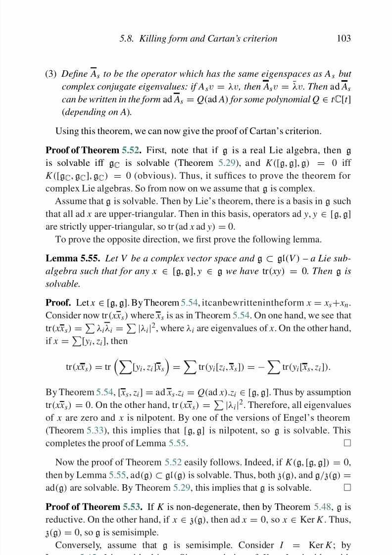
8/21/2019 Introduction to Lie Groups and Lie Algebras
http://slidepdf.com/reader/full/introduction-to-lie-groups-and-lie-algebras 115/236
5.8. Killing form and Cartan’s criterion 103
(3) Define As to be the operator which has the same eigenspaces as A s but
complex conjugate eigenvalues: if Asv
= λv , then Asv
= λv. Then ad As
can be written in the form ad As = Q(ad A) for some polynomial Q ∈ t C[t ](depending on A).
Using this theorem, we can now give the proof of Cartan’s criterion.
Proof of Theorem 5.52. First, note that if g is a real Lie algebra, then g
is solvable iff gC is solvable (Theorem 5.29), and K ([g, g], g) = 0 iff
K ([gC, gC], gC) = 0 (obvious). Thus, it suffices to prove the theorem for
complex Lie algebras. So from now on we assume that g is complex.
Assume that g is solvable. Then by Lie’s theorem, there is a basis in g such
that all ad x are upper-triangular. Then in this basis, operators ad y, y ∈ [g, g]are strictly upper-triangular, so tr(ad x ad y) = 0.
To prove the opposite direction, we first prove the following lemma.
Lemma 5.55. Let V be a complex vector space and g ⊂ gl(V ) – a Lie sub-
algebra such that for any x ∈ [g, g], y ∈ g we have tr( xy) = 0. Then g is
solvable.
Proof. Let x ∈ [g, g]. By Theorem 5.54, itcanbewrittenintheform x = x s+ x n.
Consider now tr( xx s) where x s is as in Theorem 5.54. On one hand, we see that
tr( xx s) = λiλi = |λi|2, where λi are eigenvalues of x . On the other hand,
if x =[ yi, zi], then
tr( xx s) = tr
[ yi, zi] x s
=
tr( yi[ zi, x s]) = −
tr( yi[ x s, zi]).
By Theorem 5.54, [ x s, zi] = ad x s. zi = Q(ad x ). zi ∈ [g, g]. Thus by assumption
tr( xx s) = 0. On the other hand, tr( xx s) = |λi|2. Therefore, all eigenvalues
of x are zero and x is nilpotent. By one of the versions of Engel’s theorem
(Theorem 5.33), this implies that [g, g] is nilpotent, so g is solvable. This
completes the proof of Lemma 5.55.
Now the proof of Theorem 5.52 easily follows. Indeed, if K (g, [g, g]) = 0,
then by Lemma 5.55, ad(g)
⊂ gl(g) is solvable. Thus, both z(g), and g/ z(g)
=ad(g) are solvable. By Theorem 5.29, this implies that g is solvable.
P f f Th 5 53 If K i d h b Th 5 48 i
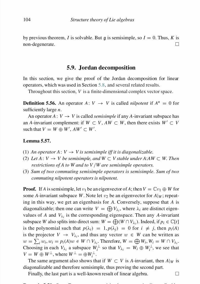
8/21/2019 Introduction to Lie Groups and Lie Algebras
http://slidepdf.com/reader/full/introduction-to-lie-groups-and-lie-algebras 116/236
104 Structure theory of Lie algebras
by previous theorem, I is solvable. But g is semisimple, so I = 0. Thus, K is
non-degenerate.
5.9. Jordan decomposition
In this section, we give the proof of the Jordan decomposition for linear
operators, which was used in Section 5.8, and several related results.
Throughout this section, V is a finite-dimensional complex vector space.
Definition 5.56. An operator A : V → V is called nilpotent if An = 0 for
sufficiently large n.
An operator A : V → V is called semisimple if any A-invariant subspace has
an A-invariant complement: if W ⊂ V , AW ⊂ W , then there exists W ⊂ V
such that V = W ⊕ W , AW ⊂ W .
Lemma 5.57.
(1) An operator A : V → V is semisimple iff it is diagonalizable.
(2) Let A : V → V be semisimple, and W ⊂ V stable under A: AW ⊂ W. Then
restrictions of A to W and to V /W are semisimple operators.
(3) Sum of two commuting semisimple operators is semisimple. Sum of two
commuting nilpotent operators is nilpotent.
Proof. If A is semisimple, let v1 be an eigenvector of A; then V = Cv1 ⊕ W for
some A-invariant subspace W . Note let v2 be an eigenvector for A
|W ; repeat-
ing in this way, we get an eigenbasis for A. Conversely, suppose that A is
diagonalizable; then one can write V = V λi, where λi are distinct eigen-
values of A and V λi is the corresponding eigenspace. Then any A-invariant
subspace W also splits into direct sum: W = (W ∩ V λi
). Indeed, if pi ∈ C[t ]is the polynomial such that p(λi) = 1, p(λ j) = 0 for i = j, then pi( A)
is the projector V → V λi , and thus any vector w ∈ W can be written as
w = i wi, wi = pi( A)w ∈ W ∩ V λi
. Therefore, W =
W i, W i = W ∩ V λi.
Choosing in each V λi a subspace W ⊥i so that V λi = W i ⊕ W ⊥i , we see thatV = W ⊕ W ⊥, where W ⊥ = ⊕W ⊥i .
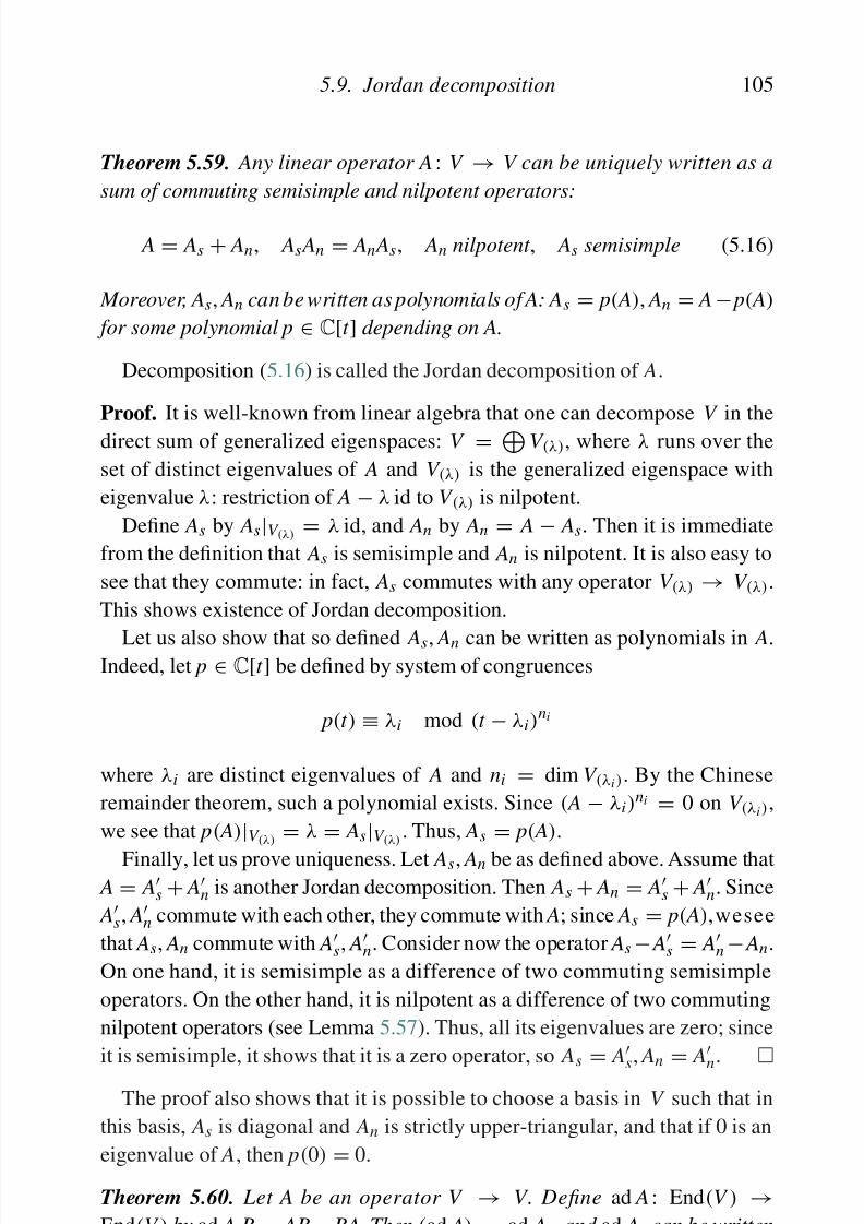
8/21/2019 Introduction to Lie Groups and Lie Algebras
http://slidepdf.com/reader/full/introduction-to-lie-groups-and-lie-algebras 117/236
5.9. Jordan decomposition 105
Theorem 5.59. Any linear operator A : V → V can be uniquely written as a
sum of commuting semisimple and nilpotent operators:
A = As + An, As An = An As, An nilpotent , As semisimple (5.16)
Moreover, As, An can be written as polynomials of A: As = p( A), An = A − p( A)
for some polynomial p ∈ C[t ] depending on A.
Decomposition (5.16) is called the Jordan decomposition of A.
Proof. It is well-known from linear algebra that one can decompose V in the
direct sum of generalized eigenspaces: V = V (λ), where λ runs over the
set of distinct eigenvalues of A and V (λ) is the generalized eigenspace with
eigenvalue λ: restriction of A − λ id to V (λ) is nilpotent.
Define As by As|V (λ) = λ id, and An by An = A − As. Then it is immediate
from the definition that As is semisimple and An is nilpotent. It is also easy to
see that they commute: in fact, As commutes with any operator V (λ) → V (λ).
This shows existence of Jordan decomposition.
Let us also show that so defined As, An can be written as polynomials in A.Indeed, let p ∈ C[t ] be defined by system of congruences
p(t ) ≡ λi mod (t − λi)ni
where λi are distinct eigenvalues of A and ni = dim V (λi ). By the Chinese
remainder theorem, such a polynomial exists. Since ( A − λi)ni = 0 on V (λi ),
we see that p( A)
|V (λ)
= λ
= As
|V (λ)
. Thus, As
= p( A).
Finally, let us prove uniqueness. Let As, An be as defined above. Assume that A = A
s + An is another Jordan decomposition. Then As + An = A
s + An. Since
As, A
n commute with each other, they commute with A; since As = p( A),wesee
that As, An commute with As, A
n. Consider now the operator As − As = A
n − An.
On one hand, it is semisimple as a difference of two commuting semisimple
operators. On the other hand, it is nilpotent as a difference of two commuting
nilpotent operators (see Lemma 5.57). Thus, all its eigenvalues are zero; since
it is semisimple, it shows that it is a zero operator, so As
= A
s
, An
= A
n
.
The proof also shows that it is possible to choose a basis in V such that in
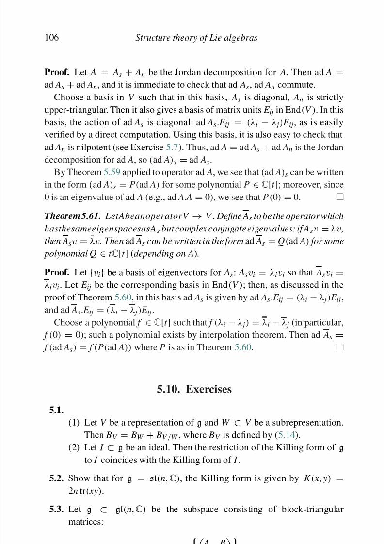
8/21/2019 Introduction to Lie Groups and Lie Algebras
http://slidepdf.com/reader/full/introduction-to-lie-groups-and-lie-algebras 118/236
106 Structure theory of Lie algebras
Proof. Let A = As + An be the Jordan decomposition for A. Then ad A =ad As
+ad An, and it is immediate to check that ad As, ad An commute.
Choose a basis in V such that in this basis, As is diagonal, An is strictly
upper-triangular. Then it also gives a basis of matrix units E ij in End(V ). In this
basis, the action of ad As is diagonal: ad As. E ij = (λi − λ j) E ij, as is easily
verified by a direct computation. Using this basis, it is also easy to check that
ad An is nilpotent (see Exercise 5.7). Thus, ad A = ad As + ad An is the Jordan
decomposition for ad A, so (ad A)s = ad As.
By Theorem 5.59 applied to operator ad A, we see that (ad A)s can be written
in the form (ad A)s =
P(ad A) for some polynomial P ∈C
[t ]; moreover, since
0 is an eigenvalue of ad A (e.g., ad A. A = 0), we see that P(0) = 0.
Theorem 5.61. LetAbeanoperatorV → V . Define As to be the operator which
hasthesameeigenspacesasAs but complex conjugate eigenvalues: if Asv = λv ,
then Asv = λv. Then ad As can be written in the form ad As = Q(ad A) for some
polynomial Q ∈ t C[t ] (depending on A).
Proof. Let {vi} be a basis of eigenvectors for As: Asvi = λivi so that Asvi =λivi. Let E ij be the corresponding basis in End(V ); then, as discussed in theproof of Theorem 5.60, in this basis ad As is given by ad As. E ij = (λi − λ j) E ij ,
and ad As. E ij = (λi − λ j) E ij.
Choose a polynomial f ∈ C[t ] such that f (λi − λ j) = λi − λ j (in particular,
f (0) = 0); such a polynomial exists by interpolation theorem. Then ad As = f (ad As) = f (P(ad A)) where P is as in Theorem 5.60.
5.10. Exercises
5.1.
(1) Let V be a representation of g and W ⊂ V be a subrepresentation.
Then BV = BW + BV /W , where BV is defined by (5.14).
(2) Let I ⊂ g be an ideal. Then the restriction of the Killing form of g
to I coincides with the Killing form of I .
5.2. Show that for g = sl(n,C), the Killing form is given by K ( x , y) =2n tr(xy).
8/21/2019 Introduction to Lie Groups and Lie Algebras
http://slidepdf.com/reader/full/introduction-to-lie-groups-and-lie-algebras 119/236
5.10. Exercises 107
where A is a k ×k matrix, B is a k ×(n−k ) matrix, and D is a (n−k )×(n−k )
matrix.
(1) Show that g is a Lie subalgebra (this is a special case of so-called
parabolic subalgebras).
(2) Show that radical of g consists of matrices of the form
λ · I B
0 µ · I
,
and describe g/ rad(g).
5.4. Show that the bilinear form tr( xy) on sp(n,K) is non-degenerate.
5.5. Let g be a real Lie algebra with a positive definite Killing form. Show
that then g = 0. [Hint: g ⊂ so(g).]
5.6. Let g be a simple Lie algebra.
(1) Show that the invariant bilinear form is unique up to a factor. [Hint:
use Exercise 4.5.]
(2) Show that g g∗ as representations of g.
5.7. Let V be a finite-dimensional complex vector space and let A : V → V
be an upper-triangular operator. Let F
k
⊂ End(V ), −n ≤ k ≤ n be thesubspace spanned by matrix units E ij with i − j ≤ k . Show that then
ad A.F k ⊂ F k −1 and thus, ad A : End(V ) → End(V ) is nilpotent.
8/21/2019 Introduction to Lie Groups and Lie Algebras
http://slidepdf.com/reader/full/introduction-to-lie-groups-and-lie-algebras 120/236
6
Complex semisimple Lie algebras
In this chapter, we begin the study of semisimple Lie algebras and their repre-
sentations. This is one of the highest achievements of the theory of Lie algebras,
which has numerous applications (for example, to physics), not to mention that
it is also one of the most beautiful areas of mathematics.
Throughout this chapter, g is a finite-dimensional semisimple Lie algebra
(see Definition 5.35); unless specified otherwise, g is complex.
6.1. Properties of semisimple Lie algebras
Cartan’s criterion of semimplicity, proved in Section 5.8, is not very conve-
nient for practical computations. However, it is extremely useful for theoretical
considerations.
Proposition 6.1. Let g be a real Lie algebra and gC – its complexification (see Definition 3.49). Then g is semisimple iff gC is semisimple.
Proof. Immediately follows from Cartan’s criterion of semisimplicity.
Remark 6.2. This theorem fails if we replace the word “semisimple” by “sim-
ple”: there exist simple real Lie algebras g such that gC is a direct sum of two
simple algebras.
Theorem 6.3. Let g be a semisimple Lie algebra, and I ⊂ g – an ideal. Thenthere is an ideal I such that g = I ⊕ I .
8/21/2019 Introduction to Lie Groups and Lie Algebras
http://slidepdf.com/reader/full/introduction-to-lie-groups-and-lie-algebras 121/236
6.1. Properties of semisimple Lie algebras 109
Corollary 6.4. A Lie algebra is semisimple iff it is a direct sum of simple Lie
algebras.
Proof. Any simple Lie algebra is semisimple by Lemma 5.37, and it is imme-
diate from Cartan criterion that the direct sum of semisimple Lie algebras is
semisimple. This proves one direction.
The opposite direction – that each semisimple algebra is a direct sum of
simple ones – easily follows by induction from the previous theorem.
Corollary 6.5. If g is a semisimple Lie algebra, then [g, g] = g.
Indeed, for a simple Lie algebra it is clear because [g, g] is an ideal in g which
can not be zero (otherwise, g would be abelian).
Proposition 6.6. Let g = g1 ⊕ · · · ⊕ gk be a semisimple Lie algebra, with gi
being simple. Then any ideal I in g is of the form I = i∈ J gi for some subset
J ⊂ {1, . . . , k }.
Note that it is not an “up to isomorphism” statement: I is not just isomorphic
to sum of some of gi but actually equal to such a sum as a subspace in g.
Proof. The proof goes by induction in k . Let πk : g → gk be the projection.
Consider πk ( I ) ⊂ gk . Since gk is simple, either πk ( I ) = 0, in which case
I ⊂ g1 ⊕ · · · ⊕ gk −1 and we can use induction assumption, or πk ( I ) = gk .
Then [gk , I ] = [gk , πk ( I )] = gk . Since I is an ideal, I ⊃ gk , so I = I ⊕ gk for
some subspace I ⊂ g1 ⊕ · · · ⊕ gk −1. It is immediate that then I is an ideal in
g1 ⊕· · ·⊕gk −1 and the result again follows from the induction assumption.
Corollary 6.7. Any ideal in a semisimple Lie algebra is semisimple. Also, anyquotient of a semisimple Lie algebra is semisimple.
Finally, recall that we have denoted by Der g the Lie algebra of all deriva-
tions of g (see (3.14)) and by Aut g the group of all automorphisms of g (see
Example 3.33).
Proposition 6.8. If g is a semisimple Lie algebra, and G–a connected Lie
group with Lie algebra g , then Der g
= g , and Aut g/ Ad G is discrete, where
Ad G = G/ Z (G) is the adjoint group associated with G (see (3.15) ).
P f R ll h f d i d i i Thi i
8/21/2019 Introduction to Lie Groups and Lie Algebras
http://slidepdf.com/reader/full/introduction-to-lie-groups-and-lie-algebras 122/236
110 Complex semisimple Lie algebras
Let us now extend the Killing form of g to Der g by letting K (δ1, δ2) =trg(δ1δ2) and consider the orthogonal complement I
= g⊥
⊂ Der g. Since K is
invariant, I is an ideal; since restriction of K to g is non-degenerate, I ∩ g = 0.
Thus, Der g = g ⊕ I ; since both g, I are ideals, we have [ I , g] = 0, which
implies that for every δ ∈ I , x ∈ g, we have ad(δ( x )) = [δ, ad x ] = 0, so
δ( x ) = 0. Thus, I = 0.
Since Aut g is a Lie group with Lie algebra Der g (see Example 3.33), the
second statement of the theorem immediately follows from the first one.
6.2. Relation with compact groups
In Section 5.8, we have shown that the Killing form of g is non-degenerate
if and only if g is semisimple. However, in the case of real g, one might also
ask whether the Killing form is positive definite, negative definite, or neither.
More generally, the same question can be asked about the trace form in any
representation: BV ( x , y) = trV ( xy).
It turns out that the answer to this question is closely related to the question
of compactness of the corresponding Lie group.
Example 6.9. Let g = u(n) be the Lie algebra of the unitary group, i.e. the Lie
algebra of skew-Hermitian matrices. Then the form ( x , y) = tr( xy) is negative
definite.
Indeed, tr( xy) = − tr( xyt ), and tr( x 2) = − tr( xx t ) = − | x ij|2 ≤ 0, with
equality only for x = 0.
Theorem 6.10. Let G be a compact real Lie group. Then g = Lie(G) is reduc-tive, and the Killing form of g is negative semidefinite, with Ker K = z(g) (the
center of g); the Killing form of the semisimple part g/ z(g) is negative definite.
Conversely, let g be a semisimple real Lie algebra with a negative definite
Killing form. Then g is a Lie algebra of a compact real Lie group.
Proof. If G is compact, then by Theorem 4.40, every complex representation
ρ : G → GL(V ) of G is unitary, so ρ (G) ⊂ U (V ), ρ(g) ⊂ u(V ) (where U (V )
is the group of unitary operators V → V ). By Example 6.9, this implies thatthe trace form BV ( x , y) is negative semidefinite, with Ker BV = Ker ρ.
A l i hi h l ifi d dj i i V h
8/21/2019 Introduction to Lie Groups and Lie Algebras
http://slidepdf.com/reader/full/introduction-to-lie-groups-and-lie-algebras 123/236
6.2. Relation with compact groups 111
of the group Aut g (see Proposition 6.8), and Aut g ⊂ GL(g) is a closed Lie
subgroup (see Example 3.33), Ad(G) is a closed Lie subgroup in the compact
group SO(g). Thus, Ad(G) is a compact Lie group. Since Ad(G) = G/ Z (G),
we have Lie(Ad(G)) = g/ z(g) = g, which proves the theorem.
Remark 6.11. In fact, one can prove a stronger result: if g is a real Lie algebra
with negative definite Killing form, then any connected Lie group with Lie
algebra g is compact. In particular, the simply-connected Lie group with Lie
algebra g is compact.
One might also ask for which real Lie algebras the Killing form is positive
definite. Unfortunately, it turns out that there are not many such algebras.
Lemma 6.12. If g is a real Lie algebra with a positive definite Killing form,
then g = 0.
The proof of this lemma is given as an exercise (Exercise 5.5).
Finally, let us discuss the relation between complex semisimple Lie algebrasand compact groups. It turns out that the only compact complex Lie groups
are tori (see Exercise 3.19). Instead, we could take real compact Lie groups
and corresponding Lie algebras, then consider their complexifications. By The-
orem 6.10, such complex Lie algebras will be reductive. A natural question
is whether any reductive complex Lie algebra can be obtained in this way.
The following theorem (which for simplicity is stated only for semisimple Lie
algebras) provides the answer.
Theorem 6.13. Let g be a complex semisimple Lie algebra. Then there exists a
real subalgebra k such that g = k ⊗ C and k is a Lie algebra of a compact Lie
group K. The Lie algebra k is called the compact real form of g; it is unique up
to conjugation.
If G is a connected complex Lie group with Lie algebra g , then the compact
group K can be chosen so that K ⊂ G. In this case, K is called the compact
real form of the Lie group G.
Th f f thi th ill t b i h I t t d d fi d
8/21/2019 Introduction to Lie Groups and Lie Algebras
http://slidepdf.com/reader/full/introduction-to-lie-groups-and-lie-algebras 124/236
112 Complex semisimple Lie algebras
6.3. Complete reducibility of representations
In this section, we will show one of fundamental results of the theory of semisim-ple Lie algebras: every representation of a semisimple Lie algebra is completely
reducible. Throughout this section, g is a semisimple complex Lie algebra and
V – a finite-dimensional complex representation of g.
This result can be proved in several ways. Historically, the first proof of this
result was given by H. Weyl using the theory of compact groups. Namely, if g is
a semisimple complex Lie algebra, then by Theorem 6.13 g can be written as a
complexification of a real Lie algebra k
= Lie(K ) for some compact-connected,
simply-connected group K . Then complex representations of g, k and K are thesame, and by Theorem 4.40, every representation of K is completely reducible.
This argument is commonly called “Weyl’s unitary trick”.
However, there is a completely algebraic proof of complete reducibility. It
uses some basic homological algebra: obstruction to complete reducibility is
described by a certain type of cohomology, and we will show that this cohomol-
ogy vanishes. To do so, we will use a special central element in the universal
enveloping algebra, called the Casimir element .
Proposition 6.15. Let g be a Lie algebra, and B – a non-degenerate invariant
symmetric bilinear form on g. Let x i be a basis of g , and x i – the dual basis with
respect to B. Then the element
C B =
x i x i ∈ U g
does not depend on the choice of the basis x i and is central. It is called theCasimir element determined by form B.
In particular, if g is semisimple and K is the Killing form, then the element
C K ∈ U g is called simply the Casimir element.
Proof. Independence of choice of basis follows from the fact that the element
I = x i ⊗ x i ∈ g ⊗ g is independent of the choice of basis: under the
identification g ⊗ g g ⊗ g∗ = End(g) given by the form B, this element
becomes the identity operator in End(g).This also shows that I = x i ⊗ x i is ad g–invariant: indeed, iden-
ifi i ∗ E d( ) i hi f
8/21/2019 Introduction to Lie Groups and Lie Algebras
http://slidepdf.com/reader/full/introduction-to-lie-groups-and-lie-algebras 125/236
6.3. Complete reducibility of representations 113
Example 6.16. Let g = sl(2,C) with the bilinear form defined by ( x , y) =tr( xy). Then the Casimir operator is given by C
= 12
h2
+ fe
+ef (compare with
Example 5.6, where centrality of C was shown by a direct computation).
Remark 6.17. Note that if g is simple, then by Exercise 4.5, the invariant
bilinear form is unique up to a constant: any such form is a multiple of the
Killing form. Thus, in this case the Casimir element is also unique up to a
constant.
Proposition 6.18. Let V be a non-trivial irreducible representation of a
semisimple Lie algebra g. Then there exists a central element C V ∈ Z (U g)which acts by a non-zero constant in V and which acts by zero in the trivial
representation.
Proof. Let BV ( x , y) = trV (ρ( x )ρ( y); by Proposition 5.47, this form is an
invariant bilinear form. If BV is non-degenerate, then let C V = C BV be the
Casimir element of g defined by form BV . Obviously, C V acts by zero in C.
Since V is irreducible, by Schur lemma C V acts in V by a constant: C V = λ idV .
On the other hand, tr(C V ) = tr( x i x
i
) = dim g, because by definition of B, tr( x i x i) = B( x i, x i) = 1. Thus, λ = dim gdim V
= 0, which proves the proposition
in this special case.
In general, let I = Ker BV ⊂ g. Then it is an ideal in g, and I = g (otherwise,
by Lemma 5.55, ρ(g) ⊂ gl(V ) is solvable, which is impossible as it is a
quotient of a semisimple Lie algebra and thus itself semisimple). By results of
Theorem 6.3, g = I ⊕ g for some non-zero ideal g ⊂ g. By Proposition 6.6,
g is semisimple, and restriction of BV to g is non-degenerate. Let C V be the
Casimir element of g corresponding to the form BV . Since I , g commute, C V
will be central in U g, and the same argument as before shows that it acts in V
by dim g
dim V = 0, which completes the proof.
Remark 6.19. In fact, a stronger result is known: if we let C be the Casimir
element defined by the Killing form, then C acts by a non-zero constant in any
nontrivial irreducible representation. However, this is slightly more difficult to
prove.
Now we are ready to prove the main result of this section.
8/21/2019 Introduction to Lie Groups and Lie Algebras
http://slidepdf.com/reader/full/introduction-to-lie-groups-and-lie-algebras 126/236
114 Complex semisimple Lie algebras
as for modules over an associative algebra. In fact, the same definition works
for any abelian category, i.e. a category where morphisms form abelian groups
and where we have the notion of image and kernel of a morphism satisfying
the usual properties.
In particular, the standard argument of homological agebra shows that for
fixed V 1, V 2 equivalence classes of extensions 0 → V 1 → W → V 2 → 0 are
in bijection with Ext1(V 2, V 1). Thus, our goal is to show that Ext1(V 2, V 1) = 0
for any two representations V 1, V 2. This will be done in several steps. For
convenience, we introduce the notation H 1(g, V ) = Ext1(C, V ).
Lemma 6.21. For any irreducible representation V , one has H 1(g, V ) = 0.
Proof. To prove that Ext1(C, V ) = 0 it suffices to show that every short exact
sequence of the form 0 → V → W → C→ 0 splits. So let us assume that we
have such an exact sequence.
Let us consider separately two cases: V is a non-trivial irreducible represen-
tation and V = C.
If V is a non-trivial irreducible representation, consider the Casimir element
C V as defined in Proposition 6.18. Since it acts in C by zero and in V by a
non-zero constant λ, its eigenvalues in W are 0 with multiplicity 1 and λ with
multiplicity dim V . Thus, W = V ⊕ W 0, where W 0 is the eigenspace for C V
with eigenvalue 0 (which must be one-dimensional). Since C V is central, W 0
is a subrepresentation; since the kernel of the projection W → C is V , it gives
an isomorphism W 0 C. Thus, W V ⊕ C.
If V = C is a trivial representation, so we have an exact sequence 0 → C→W → C→ 0, then W is a two-dimensional representation such that the actionof ρ( x ) is strictly upper triangular for all x ∈ g. Thus, ρ (g) is nilpotent, so by
Corollary 6.7, ρ (g) = 0. Thus, W C⊕ C as a representation.
This lemma provides the crucial step; the rest is simple homological algebra.
Lemma 6.22. H 1(g, V ) = 0 for any representation V .
Proof. If we have a short exact sequence of representations 0
→ V 1
→ V
→V 2 → 0, then we have a long exact sequence of Ext groups; in particular,

8/21/2019 Introduction to Lie Groups and Lie Algebras
http://slidepdf.com/reader/full/introduction-to-lie-groups-and-lie-algebras 127/236
6.3. Complete reducibility of representations 115
We are now ready to prove Theorem 6.20. Let 0 → V 1 → W → V 2 → 0
be a short exact sequence of g-modules. We need to show that it splits.
Let us apply to this sequence the functor X → HomC(V 2, X ) = V ∗2 ⊗ X
(considered as a g-module, see Example 4.12). Obviously, this gives a short
exact sequence of g-modules
0 → HomC(V 2, V 1) → HomC(V 2, W ) → HomC(V 2, V 2) → 0
Now, let us apply to this sequence the functor of g-invariants: X → X g =Homg(C, X ). Applying this functor to HomC( A, B) gives (HomC( A, B))g
=Homg( A, B) (see Example 4.14).This functor is left exact but in general not exact, so we get a long exact
sequence
0 → Homg(V 2, V 1) → Homg(V 2, W ) → Homg(V 2, V 2)
→ Ext1(C, V ∗2 ⊗ V 1) = H 1(g, V ∗2 ⊗ V 1) → . . .
But since we have already proved that H 1(g, V )
= 0 for any module V , we see
that in fact we do have a short exact sequence
0 → Homg(V 2, V 1) → Homg(V 2, W ) → Homg(V 2, V 2) → 0
In particular, this shows that there exists a morphism f : V 2 → W which, when
composed with projection W → V 2, gives identity morphism V 2 → V 2. This
gives a splitting of exact sequence 0 → V 1 → W → V 2 → 0. This completes
the proof of Theorem 6.20.
Remark 6.23. The same proof can be rewritten without using the language
of Ext groups; see, for example, [46]. This would make it formally accessible
to readers with no knowledge of homological algebra. However, this does not
change the fact that all arguments are essentially homological in nature; in fact,
such a rewriting would obscure the ideas of the proof rather than make them
clearer.
The groups Ext
1
(V , W ) and in particular, H
1
(g, V ) = Ext
1
(C
, V ) used inthis proof are just the beginning of a well-developed cohomology theory of Lie
l b I i l d fi hi h h l H i( V ) i
8/21/2019 Introduction to Lie Groups and Lie Algebras
http://slidepdf.com/reader/full/introduction-to-lie-groups-and-lie-algebras 128/236
116 Complex semisimple Lie algebras
where H i(G,R) are the usual topological cohomology (which can be defined,
for example, as De Rham cohomology). We refer the reader to [12] for an
introduction to this theory.
Complete reducibility has a number of useful corollaries. One of them is the
following result, announced in Section 5.6.
Theorem 6.24. Any reductive Lie algebra can be written as a direct sum (as a
Lie algebra) of semisimple and commutative ideals:
g = z ⊕ gss, z commutative, gss semisimple.
Proof. Consider the adjoint representation of g. Since the center z(g) acts by
zero in an adjoint representation, the adjoint action descends to an action of
g = g/ z(g). By definition of a reductive algebra, g is semisimple. Thus, g
considered as a representation of g is completely reducible. Since z ⊂ g is
stable under adjoint action, it is a subrepresentation. By complete reducibility,
we can write g = z ⊕ I for some I ⊂ g such that ad x . I ⊂ I for any x ∈ g.
Thus, I is an ideal in g, so g
= z
⊕ I as Lie algebras. Obviously, I
g/ z
= g
is semisimple.
In a similar way one can prove Levi theorem (Theorem 5.41). We do not give
this proof here, referring the reader to [24, 41, 46]. Instead, we just mention
that in the language of homological algebra, the Levi theorem follows from the
vanishing of cohomology H 2(g,C).
6.4. Semisimple elements and toral subalgebrasRecall that the main tool used in the study of representations of sl(2,C) in
Section 4.8 was the weight decomposition, i.e. decomposing a representation
of sl(2,C) into direct sum of eigenspaces for h. In order to generalize this idea
to other Lie algebras, we need to find a proper analog of h.
Looking closely at the proofs of Section 4.8, we see that the key property of
h was the commutation relations [h, e] = 2e, [h, f ] = −2 f which were used to
to show that e, f shift the weight. In other words, ad h is diagonal in the basise, f , h. This justifies the following definition.
8/21/2019 Introduction to Lie Groups and Lie Algebras
http://slidepdf.com/reader/full/introduction-to-lie-groups-and-lie-algebras 129/236
6.4. Semisimple elements and toral subalgebras 117
Of course, we do not yet know if such elements exist for any g. The following
theorem, which generalizes Jordan decomposition theorem (Theorem 5.59),
answers this question.
Theorem 6.26. If g is a semisimple complex Lie algebra, then any x ∈ g can
be uniquely written in the form
x = x s + x n,
where x s is semisimple, x n is nilpotent, and [ x s, x n] = 0. Moreover, if for some
y ∈
g we have[ x , y
] = 0 , then
[ x
s, y
] = 0.
Proof. Uniqueness immediately follows from the uniqueness of the Jordan
decomposition for ad x (Theorem 5.59): if x = x s + x n = x s + x n, then (ad x )s =ad x s = ad x s, so ad( x s − x s) = 0. But by definition, a semisimple Lie algebra
has zero center, so this implies x s − x s = 0.
To prove existence, let us write g as direct sum of generalized eigenspaces
for ad x : g =
gλ, (ad x − λ id)n|gλ
= 0 for n 0.
Lemma 6.27. [gλ, gµ] ⊂ gλ+µ.
Proof. By Jacobi identity, (ad x − λ − µ)[ y, z] = [(ad x − λ) y, z] + [ y, (ad x −µ) z]. Thus, if y ∈ gλ, z ∈ gµ, then induction gives
(ad x − λ − µ)n[ y, z] =
k
n
k
[(ad x − λ)k y, (ad x − µ)n−k z],
which is zero for n > dim gλ
+dim gµ.
Let ad x = (ad x )s+(ad x )n be the Jordan decomposition of operator ad x (see
Theorem 5.59), so that (ad x )s|gλ = λ. Then the lemma implies that (ad x )s is a
derivation of g. By Proposition 6.8, any derivation is inner, so (ad x )s = ad x s
for some x s ∈ g; thus, (ad x )n = ad( x − x s). This proves the existence of the
Jordan decomposition for x . It also shows that if ad x . y = 0, then (ad x )s. y =(ad x s). y = 0.
Corollary 6.28. In any semisimple complex Lie algebra, there exist non-zerosemisimple elements.

8/21/2019 Introduction to Lie Groups and Lie Algebras
http://slidepdf.com/reader/full/introduction-to-lie-groups-and-lie-algebras 130/236
118 Complex semisimple Lie algebras
Definition 6.29. A subalgebra h ⊂ g is called toral if it is commutative and
consists of semisimple elements.
Theorem 6.30. Let g be a complex semisimple Lie algebra, h ⊂ g a toral
subalgebra, and let ( , ) be a non-degenerate invariant symmetric bilinear form
on g ( for example, the Killing form). Then
(1) g = α∈h∗ gα , where gα is a common eigenspace for all operators
ad h, h ∈ h , with eigenvalue α:
ad h. x =
α, h x , h
∈ h, x
∈ g
α.
In particular, h ⊂ g0.
(2) [gα, gβ] ⊂ gα+β .
(3) If α + β = 0 , then gα, gβ are orthogonal with respect to the form ( , ).
(4) For any α , the form ( , ) gives a non-degenerate pairing gα ⊗ g−α → C.
Proof. By definition, for each h ∈ h, the operator ad h is diagonalizable. Since
all operators ad h commute, they can be simultaneously diagonalized, which
is exactly the statement of the first part of the theorem. Of course, since g is
finite-dimensional, gα = 0 for all but finitely many α ⊂ h∗.
The second part is in fact a very special case of Lemma 6.27. However, in
this case it can be proved much easier: if y ∈ gα, z ∈ gβ , then
ad h.[ y, z] = [ad h. y, z] + [ y, ad h. z] = α, h[ y, z]
+ β, h
[ y, z
] = α
+β, h
[ y, z
].
For the third part, notice that if x ∈ gα, y ∈ gβ , h ∈ h, then invariance of the
form shows that ([h, x ], y) + ( x , [h, y]) = (h, α + h, β)( x , y) = 0; thus, if
( x , y) = 0, then h, α + β = 0 for all h, which implies α + β = 0.
The final part immediately follows from the previous part.
For future use, we will also need some information about the zero eigenvalue
subspace g0.
Lemma 6.31. In the notation of Theorem 6.30 , we have
8/21/2019 Introduction to Lie Groups and Lie Algebras
http://slidepdf.com/reader/full/introduction-to-lie-groups-and-lie-algebras 131/236
6.5. Cartan subalgebra 119
To prove part (2), note that if x ∈ g0, then [ x , h] = 0 for all h ∈ h. But then,
by Theorem 6.26,
[ x s, h
] = 0, so x s
∈ g0.
To prove the last part, consider g as a representation of g0. Then the
trace form ( x 1, x 2) = trg(ad x 1 ad x 2) on g0 is exactly the restriction of
the Killing form K g to g0 and by part (1) is non-degenerate. But by
one of the forms of Cartan’s criterion (Theorem 5.48), this implies that g
is reductive.
6.5. Cartan subalgebra
Our next goal is to produce as large a toral subalgebra in g as possible. The
standard way of formalizing this is as follows.
Definition 6.32. Let g be a complex semisimple Lie algebra. A Cartan sub-
algebra h ⊂ g is a toral subalgebra which coincides with its centralizer:
C (h) = { x | [ x , h] = 0} = h.
Remark 6.33. This definition should only be used for semisimple Lie algebras:
for general Lie algebras, Cartan subalgebras are defined in a different way (see,
e.g., [47]). However, it can be shown that for semisimple algebras our definition
is equivalent to the usual one. (Proof in one direction is given in Exercise 6.3.)
Example 6.34. Let g = sl(n,C) and h = {diagonal matrices with trace 0}.
Then h is a Cartan subalgebra. Indeed, it is obviously commutative, and every
diagonal element is semisimple (see Exercise 6.2), so it is a toral subalgebra. On
the other hand, choose h
∈ h to be a diagonal matrix with distinct eigenvalues.
By a well-known result of linear algebra, if [ x , h] = 0, and h has distinct
eigenvalues, then any eigenvector of h is also an eigenvector of x ; thus, x must
also be diagonal. Thus, C (h) = h.
We still need to prove existence of Cartan subalgebras.
Theorem 6.35. Let h ⊂ g be a maximal toral subalgebra, i.e. a toral subalgebra
which is not properly contained in any other toral subalgebra. Thenh isaCartan
subalgebra.
P f L
b h d i i f i i f d h
8/21/2019 Introduction to Lie Groups and Lie Algebras
http://slidepdf.com/reader/full/introduction-to-lie-groups-and-lie-algebras 132/236
120 Complex semisimple Lie algebras
(ad x s)|g0 = 0 and thus x s /∈ h. On the other hand, [h, x s] = 0 (since x s ∈ g0),
so h
⊕C
· x s would be a toral subalgebra, which contradicts maximality of h.
By Engel’s theorem (Theorem 5.34), this implies that g0 is nilpotent. On the
other hand, by Lemma 6.31, g0 is reductive. Therefore, it must be commutative.
Finally, to show that any x ∈ g0 is semisimple, it suffices to show that for
any such x , the nilpotent part x n = 0 (recall that by Lemma 6.31, x n ∈ g0).
But since ad x n is nilpotent and g0 is commutative, for any y ∈ g0, ad x n ad y
is also nilpotent, so trg(ad x n ad y) = 0. Since the Killing form on g0 is non-
degenerate (Lemma 6.31), this implies x n = 0. Thus, we see that g0 = C (h)
is a toral subalgebra which contains h. Since h was chosen to be maximal,
C (h) = h.
Corollary 6.36. In every complex semisimple Lie algebra g , there exists a
Cartan subalgebra.
Later (see Section 6.7) we will give another way of constructing Cartan
subalgebras and will prove that all Cartan subalgebras are actually conjugate in
g. In particular, this implies that they have the same dimension. This dimension
is called the rank of g:
rank (g) = dim h. (6.1)
Example 6.37. Rank of sl(n,C) is equal to n − 1.
6.6. Root decomposition and root systems
From now on, we fix a complex semisimple Lie algebra g and a Cartansubalgebra h ⊂ g.
Theorem 6.38.
(1) We have the following decomposition for g , called the root decomposition
g = h ⊕
α∈ R
gα , (6.2)
where
8/21/2019 Introduction to Lie Groups and Lie Algebras
http://slidepdf.com/reader/full/introduction-to-lie-groups-and-lie-algebras 133/236
6.6. Root decomposition and root systems 121
(3) If α + β = 0 , then gα, gβ are orthogonal with respect to the Killing
form K.
(4) For any α , the Killing form gives a non-degenerate pairing gα ⊗g−α → C.
In particular, restriction of K to h is non-degenerate.
Proof. This immediately follows from Theorem 6.30 and g0 = h, which is the
definition of Cartan subalgebra.
Theorem 6.39. Let g1 . . . gn be gi are simple Lie algebras and let g = gi.
(1) Let hi
⊂ gi be Cartan subalgebras of gi and Ri
⊂ h∗
i the corresponding
root systems of gi. Then h = hi is a Cartan subalgebra in g and the
corresponding root system is R = Ri.
(2) Each Cartan subalgebra in g must have the form h = hi where hi ⊂ gi
is a Cartan subalgebra in gi.
Proof. The first part is obvious from the definitions. To prove the second part,
let hi = πi(h), where πi : g → gi is the projection. It is immediate that for
x
∈ gi, h
∈ h, we have
[h, x
] = [πi(h), x
]. From this it easily follows that hi
is a Cartan subalgebra. To show that h = hi, notice that obviously h ⊂hi; since
hi is toral, by definition of Cartan subalgebra we must have
h = hi.
Example 6.40. Let g = sl(n,C), h = diagonal matrices with trace 0 (see
Example 6.34). Denote by ei : h → C the functional which computes ith
diagonal entry of h:
ei :
h1 0 . . .
0 h2 . . .
. . .
0 . . . hn
→ hi.
Then one easily sees that
ei = 0, so
h∗ =Cei/C
(e1 + · · · + en).
I i h i i E i f d h h h [h E ]
8/21/2019 Introduction to Lie Groups and Lie Algebras
http://slidepdf.com/reader/full/introduction-to-lie-groups-and-lie-algebras 134/236
122 Complex semisimple Lie algebras
The Killing form on h is given by
(h, h) =i= j
(hi − h j)(hi − h j) = 2ni
hihi = 2n tr(hh).
From this, it is easy to show that if λ = λiei, µ = µiei ∈ h∗, and λi, µi
are chosen so that
λi =
µi = 0 (which is always possible), then the
corresponding form on h∗ is given by
(α, µ) = 1
2n i
λiµi.
The root decomposition is the most important result one should know about
semisimple Lie algebras – much more important than the definition of semisim-
ple algebras (in fact, this could be taken as the definition, see Exercise 6.4). Our
goal is to use this decomposition to get as much information as possible about
the structure of semisimple Lie algebras, eventually getting full classification
theorem for them.
From now on, we will denote by ( , ) a non-degenerate symmetric invariantbilinear form on g. Such a form exists: for example, one can take ( , ) to be
the Killing form (in fact, if g is simple, then any invariant bilinear form is
a multiple of the Killing form, see Exercise 4.5). However, in most cases it is
more convenient to use a different normalization, which we will introduce later,
in Exercise 8.7.
Since the restriction of ( , ) to h is non-degenerate (see Theorem 6.38), it
defines an isomorphism h ∼
−→ h∗ and a non-degenerate bilinear form on h∗,
which we will also denote by ( , ). It can be explicitly defined as follows: if wedenote for α ∈ h∗ by H α the corresponding element of h, then
(α, β) = H α , β = ( H α, H β ) (6.4)
for any α , β ∈ h∗.
Lemma 6.41. Let e ∈ gα , f ∈ g−α and let H α be defined by (6.4). Then
[e, f ] = (e, f ) H α.
8/21/2019 Introduction to Lie Groups and Lie Algebras
http://slidepdf.com/reader/full/introduction-to-lie-groups-and-lie-algebras 135/236
6.6. Root decomposition and root systems 123
Lemma 6.42.
(1) Let α ∈ R. Then (α , α) = ( H α , H α ) = 0.(2) Let e ∈ gα, f ∈ g−α be such that (e, f ) = 2/(α, α) , and let
hα = 2 H α
(α, α). (6.5)
Then hα , α = 2 and the elements e, f , hα satisfy the commutation rela-
tions (3.24) of Lie algebra sl(2,C). We will denote such a subalgebra by
sl(
2,C)
α ⊂ g.
(3) So defined hα is independent of the choice of non-degenerate invariant
bilinear form ( , ).
Proof. Assume that (α, α) = 0; then H α, α = 0. Choose e ∈ gα , f ∈ g−α
such that (e, f ) = 0 (possible by Theorem 6.38). Let h = [e, f ] = (e, f ) H α
and consider the algebra a generated by e, f , h. Then we see that [h, e] =h, αe = 0, [h, f ] = −h, α f = 0, soa is solvable Lie algebra. By Lie theorem
(Theorem 5.30), we can choose a basis in g such that operators ad e, ad f , ad h
are upper triangular. Since h = [e, f ], ad h will be strictly upper-triangular and
thus nilpotent. But since h ∈ h, it is also semisimple. Thus, h = 0. On the other
hand, h = (e, f ) H α = 0. This contradiction proves the first part of the theorem.
The second part is immediate from definitions and Lemma 6.41.
The last part is left as an exercise to the reader (Exercise 6.7).
This lemma gives us a very powerful tool for study of g: we can considerg as a
module over the subalgebra sl(2,C)α and then use results about representations
of sl(2,C) proved in Section 4.8.
Lemma 6.43. Let α be a root, and let sl(2,C)α be the Lie subalgebra generated
by e ∈ gα, f ∈ g−α and hα as in Lemma 6.42.
Consider the subspace
V = Chα ⊕
k
∈Z,k
=0
gk α ⊂ g.
Then V is an irreducible representation of sl(2,C)α .
8/21/2019 Introduction to Lie Groups and Lie Algebras
http://slidepdf.com/reader/full/introduction-to-lie-groups-and-lie-algebras 136/236
124 Complex semisimple Lie algebras
Now we can prove the main theorem about the structure of semisimple Lie
algebras.
Theorem 6.44. Let g be a complex semisimple Lie algebra with Cartan subal-
gebra h and root decomposition g = h ⊕α∈ R gα . Let ( , ) a non-degenerate
symmetric invariant bilinear form on g.
(1) R spans h∗ as a vector space, and elements hα, α ∈ R, defined by (6.5) span
h as a vector space.
(2) For each α ∈ R, the root subspace gα is one-dimensional.
(3) For any two roots α, β , the number
hα , β = 2(α, β)
(α, α)
is integer.
(4) For α ∈ R, define the reflection operator sα : h∗ → h∗ by
sα(λ) = λ − hα , λα = λ − 2(α, λ)(α, α)
α.
Then for any roots α, β, sα (β) is also a root. In particular, if α ∈ R, then
−α = sα (α) ∈ R.
(5) For any root α , the only multiples of α which are also roots are ±α.
(6) For roots α, β = ±α , the subspace
V = k ∈Z
gβ+k α
is an irreducible representation of sl(2,C)α .
(7) If α , β are roots such that α + β is also a root, then [gα, gβ] = gα+β .
Proof. (1) Assume that R does not generate h∗; then there exists a non-zero
h ∈ h such that h, α = 0 for all α ∈ R. But then root decomposition
(6.2) implies that ad h = 0. However, by definition in a semisimpleLie algebra, the center is trivial: z(g) = 0.
8/21/2019 Introduction to Lie Groups and Lie Algebras
http://slidepdf.com/reader/full/introduction-to-lie-groups-and-lie-algebras 137/236
6.6. Root decomposition and root systems 125
(3) Consider g as a representation of sl(2,C)α. Then elements of gβ have
weight equal to
hα, β
. But by Theorem 4.60, weights of any finite-
dimensional representation of sl(2,C) are integer.
(4) Assume that hα, β = n ≥ 0. Then elements of gβ have weight n
with respect to the action of sl(2,C)α. By Theorem 4.60, operator f nαis an isomorphism of the space of vectors of weight n with the space of
vectors of weight −n. In particular, it means that if v ∈ gβ is non-zero
vector, then f nα v ∈ gβ−nα is also non-zero. Thus, β −nα = sα(β) ∈ R.
For n ≤ 0, the proof is similar, using e−n instead of f n .
(5) Assume that α and β=
cα, c∈C, are both roots. By part (3),
(2(α, β)/(α, α)) = 2c is integer, so c is a half-integer. The same argu-
ment shows that 1/c is also a half-integer. It is easy to see that this
implies that c ∈ {±1, ±2, ±1/2}. Interchanging the roots if necessary
and possibly replacing α by −α, we have c = 1 or c = 2.
Now let us consider the subspace
V = Chα ⊕ k ∈Z,k =0
gk α ⊂ g.
By Lemma 6.43, V is an irreducible representation of sl(2,C)α,andby
part (2), V [2] = gα = Ceα . Thus, the map ad eα : gα → g2α is zero.
But the results of Section 4.8 show that in an irreducible representation,
the kernel of e is exactly the highest weight subspace. Thus, we see
that V has highest weight 2: V [4] = V [6] = · · · = 0. This means that
V = g−α ⊕ Chα ⊕ gα, so the only integer multiples of α which are
roots are ±α. In particular, 2α is not a root.Combining these two results, we see that if α, cα are both roots,
then c = ±1.
(6) Proof is immediate from dim gβ+k α = 1.
(7) We already know that [gα, gβ] ⊂ gα+β . Since dim gα+β = 1, we need
to show that for non-zero eα ∈ gα, eβ ∈ gβ , we have [eα, eβ ] = 0.
This follows from the previous part and the fact that in an irreducible
representation of sl(2,C), if v
∈ V
[k
]is non-zero and V
[k
+2
] = 0,
then e.v = 0.
I th t h t ill t d th t f t R i d t il A ill
8/21/2019 Introduction to Lie Groups and Lie Algebras
http://slidepdf.com/reader/full/introduction-to-lie-groups-and-lie-algebras 138/236
126 Complex semisimple Lie algebras
(2) Let h∗R ⊂ h∗ be the real vector space generated by α ∈ R. Then h∗ =
h∗R
⊕ih∗R
. Also, h∗R
= {λ
∈ h∗
| λ, h
∈R for all h
∈ hR
} = (hR)∗.
Proof. Let us first prove that the restriction of the Killing form to hR is real
and positive definite. Indeed,
(hα , hβ ) = tr(ad hα ad hβ ) =γ ∈ R
hα , γ hβ , γ .
But by Theorem 6.44, hα, γ , hβ , γ ∈ Z, so (hα , hβ ) ∈ Z.
Now let h = cαhα ∈ hR. Then h, γ = cαhα, γ ∈ R for anyroot γ , so
(h, h) = tr(ad h)2 =
γ
h, γ 2 ≥ 0
which proves that the Killing form is positive definite on hR.
Since the Killing form is positive definite on hR, it is negative definite on
ihR, so hR ∩ ihR = {0}, which implies dimR hR ≤ 1
2 dimR h = r , wherer = dimC h is the rank of g. On the other hand, since hα generate h over C, we
see that dimR hR ≥ r . Thus, dimR hR = r , so h = hR ⊕ ihR.
The second part easily follows from the first one.
Remark 6.46. It easily follows from this theorem and Theorem 6.10 that if k
is a compact real form of g (see Theorem 6.13), then k∩h = ihR. For example,
for g = sl(n,C), hR consists of traceless diagonal matrices with real entries,
and su(n) ∩ h = traceless diagonal skew-hermitian matrices = ihR.
6.7. Regular elements and conjugacy of Cartan
subalgebras
In this section, we give another way of constructing Cartan subalgebras, and
prove conjugacy of Cartan subalgebras, which was stated without proof in
Section 6.5. This section can be skipped at first reading.
We start with an example.
E l 6 47 L l( C) d l h b h h ll i l f h
8/21/2019 Introduction to Lie Groups and Lie Algebras
http://slidepdf.com/reader/full/introduction-to-lie-groups-and-lie-algebras 139/236
6.7. Regular elements and conjugacy of Cartan subalgebras 127
discussed in Example 6.34, is a Cartan subalgebra in sl(n,C)) can be recovered
as the centralizer of h: h
= C (h).
This suggests a method of constructing Cartan subalgebras for an arbitrary
semisimple Lie algebra g as centralizers of the “generic” element h ∈ g. We
must, however, give a precise definition of the word “generic”, which can be
done as follows.
Definition 6.48. For any x ∈ g, define “nullity” of x by
n( x )
= multiplicity of 0 as a generalized eigenvalue of ad x
It is clear that for every x ∈ g, n( x ) ≥ 1 (because x itself is annihilated by
ad x ).
Definition 6.49. For any Lie algebra g, its rank rank (g) is defined by
rank (g) = min x ∈g n( x )
An element x ∈ g is called regular if n( x ) = rank (g).
Example 6.50. Let g = gl(n,C) and let x ∈ g have eigenvalues λi. Then
eigenvalues of ad x are λi − λ j, i, j = 1 . . . n; thus, n( x ) ≥ n with the equality
iff all λi are distinct. Therefore, rank (gl(n,C)) = n and x ∈ gl(n,C) is reg-
ular iff its eigenvalues are distinct (in which case it must be diagonalizable).
A minor modification of this argument shows that rank ( sl(n,C)) = n − 1 and
x ∈ sl(n,C) is regular iff its eigenvalues are distinct.
Lemma 6.51. In any finite-dimensional complex Lie algebra g , the set greg of
regular elements is connected, open and dense in g.
Proof. For any x ∈ g, let p x (t ) = det(ad x − t ) = an( x )t n + · · · + a0( x ) be
the characteristic polynomial of ad x . By definition, n( x ) is multiplicity of zero
as a root of p x (t ): thus, for any x , polynomial p x (t ) has zero of order ≥ r at
zero, with equality iff x is regular (r is the rank of g). Therefore, x is regular iff
ar ( x ) = 0. However, each of the coefficients ak ( x ) is a polynomial function on
g; thus, the set { x | ar ( x ) = 0} is an open dense set in g.To prove that greg is connected, note that for any affine complex line l =
8/21/2019 Introduction to Lie Groups and Lie Algebras
http://slidepdf.com/reader/full/introduction-to-lie-groups-and-lie-algebras 140/236
128 Complex semisimple Lie algebras
if x 1, x 2 ∈ greg, by taking a complex line through them we see that x 1, x 2 are
path-connected.
Proposition 6.52. Let g be a complex semisimple Lie algebra, and h ⊂ g – a
Cartan subalgebra.
(1) dim h = rank (g).
(2)
h ∩ greg = {h ∈ h | h, α = 0 ∀ α ∈ R}.
In particular, h ∩ greg is open and dense in h.
Proof. Let G be a connected Lie group with Lie algebra G and define
V = {h ∈ h | h, α = 0 ∀ α ∈ R} ⊂ h
and let U = Ad G.V . Then the set U is open in g. Indeed, consider the map
ϕ : G ×
V →
g given by (g, x ) →
Ad g. x . Then, for any x ∈
V , the corre-
sponding map of tangent spaces at (1, x ) is given by ϕ∗ : g× h → g : ( y, h) →[ y, x ]+ h. Since [gα , x ] = gα (this is where we need that x , α = 0 ∀α), we see
that ϕ∗ is surjective; therefore, the image of ϕ contains an open neighborhood
of x . Since any u ∈ U can be written in the form u = Ad g. x for some x ∈ V ,
this implies that for any u ∈ U , the set U contains an open neighborhood of u.
Since the set U is open, it must intersect with the open dense set greg. On the
other hand, for any u = Ad g. x ∈ U , we have n(u) = n( x ) = dim C ( x ), where
C ( x ) = { y ∈ g | [ x , y] = 0} is the centralizer of x , so rank (g) = n( x ). But iteasily follows from the root decomposition and the definition of V that for any
x ∈ V , we have C ( x ) = h. Therefore, rank (g) = dim h.
The second part of the proposition now immediately follows from the
observation that for any h ∈ h, we have
n(h) = dim C (h) = dim h + |{α ∈ R | h, α = 0}|.
Theorem 6.53. Let g be a complex semisimple Lie algebra, and x ∈ g – aregular semisimple element. Then the centralizer C ( x ) = { y ∈ g | [ x , y] = 0}
8/21/2019 Introduction to Lie Groups and Lie Algebras
http://slidepdf.com/reader/full/introduction-to-lie-groups-and-lie-algebras 141/236
6.7. Regular elements and conjugacy of Cartan subalgebras 129
We claim that C ( x ) is nilpotent. Indeed, by Engel’s theorem (Theorem 5.34)
it suffices to prove that for any y
∈ C ( x ), the restriction of ad y to C ( x ) is
nilpotent. Consider element x t = x + ty ∈ C ( x ). Then for small values of t ,
we have ad x t |g/g0 is invertible (since ad x |g/g0
is invertible), so the null space
of x t is contained in g0 = C ( x ). On the other hand, by definition of rank we
have n( x t ) ≥ rank (g) = dim C ( x ) (the last equality holds because x is regular).
Thus, ad x t |C ( x ) is nilpotent for t close to zero; since x acts by zero in C ( x ), this
means that ad y|C ( x ) is nilpotent.
Now the same arguments as in the proof ofTheorem 6.35 show thatg0 = C ( x )
is a toral subalgebra. Since x ∈
C ( x ), the centralizer of C ( x ) is contained in
C ( x ); thus, C ( x ) is a Cartan subalgebra.
The last part is obvious: if h is a Cartan subalgebra, then by Proposition 6.52
it contains a regular semisimple element x and thus h ⊂ C ( x ); since dim h =rank (g) = dim C ( x ), we see that h = C ( x ).
Corollary 6.54. In a complex semisimple Lie algebra:
(1) Any regular element is semisimple.
(2) Any regular element is contained in a unique Cartan subalgebra.
Proof. It is immediate from the definition that eigenvalues of ad x and ad x s =(ad x )s coincide; thus, if x is regular then so is x s. Then by Theorem 6.53, C ( x s)
is a Cartan subalgebra. Since x ∈ C ( x s), x itself must be semisimple.
To prove the second part, note that by (1) and Theorem 6.53, for any regular
x the centralizer C ( x ) is a Cartan subalgebra, so x is contained in a Cartan
subalgebra. To prove uniqueness, note that if h
x is a Cartan subalge-
bra, then commutativity of h implies that h ⊂ C ( x ). On the other hand, byProposition 6.52, dim h = rank (g) = dim C ( x ).
Theorem 6.55. Any two Cartan subalgebras in a semisimple Lie algebra are
conjugate: if h1, h2 ⊂ g are Cartan subalgebras, then there exists an element
g in the Lie group G corresponding to g such that h2 = Ad g(h1).
Proof. Consider the set greg of regular elements in g; by Corollary 6.54, any
such element is contained in a unique Cartan subalgebra, namely h x = C ( x ).Define the following equivalence relation on greg:
8/21/2019 Introduction to Lie Groups and Lie Algebras
http://slidepdf.com/reader/full/introduction-to-lie-groups-and-lie-algebras 142/236
130 Complex semisimple Lie algebras
is open. Thus, each equivalence class of x contains a neighborhood of x and
therefore is open.
Since the set greg is connected (Lemma 6.51), and each equivalence class of
relation ∼ is open, this implies that there is only one equivalence class: for any
regular x , y, corresponding Cartan subalgebras h x , h y are conjugate. Since every
Cartan subalgebra has the form h x (Theorem 6.53), this implies the statement
of the theorem.
6.8. Exercises
6.1. Show that the Casimir operator for g = so(3,R) is given by C = 12
( J 2 x + J 2 y + J 2 z ), where generators J x , J y, J z are defined in Section 3.10; thus, it
follows from Proposition 6.15 that J 2 x + J 2 y + J 2 z ∈ U so(3,R) is central.
Compare this with the proof of Lemma 4.62, where the same result was
obtained by direct computation.
6.2. Show that for g = gl(n,C), Definition 6.25 is equivalent to the usual
definition of a semisimple operator (hint: use results of Section 5.9).
6.3. Show that if h ⊂ g is a Cartan subalgebra in a complex semisimple
Lie algebra, then h is a nilpotent subalgebra which coincides with its
normalizer n(h) = { x ∈ g | ad x .h ⊂ h}. (This is the usual definition of a
Cartan subalgebra which can be used for any Lie algebra, not necessarily
a semisimple one.)
6.4. Let g be a complex Lie algebra which has a root decomposition:
g = h ⊕α∈ R
gα
where R is a finite subset in h∗ −{0}, h is commutative and for h ∈ h, x ∈gα, we have [h, x ] = h, α x . Show that then g is semisimple, and h is a
Cartan subalgebra.
6.5. Let h ⊂ so(4,C) be the subalgebra consisting of matrices of the forma
8/21/2019 Introduction to Lie Groups and Lie Algebras
http://slidepdf.com/reader/full/introduction-to-lie-groups-and-lie-algebras 143/236
6.8. Exercises 131
6.6. (1) Define a bilinear form B on W = 2C4 by ω1 ∧ω2 = B(ω1, ω2)e1 ∧e2
∧e3
∧e4. Show that B is a symmetric non-degenerate form and
construct an orthonormal basis for B.
(2) Let g = so(W , B) = { x ∈ gl(W ) | B( x ω1, ω2) + B(ω1, x ω2) = 0}.
Show that g so(6,C).
(3) Show that the form B is invariant under the natural action of sl(4,C)
on 2C4.
(4) Using results of the previous parts, construct a homomorphism
sl(4,C) → so(6,C) and prove that it is an isomorphism.
6.7. Show that definition (6.5) of hα is independent of the choice of ( , ):replacing the Killing form by any other non-degenerate symmetric invari-
ant bilinear form gives the same hα (see Exercise 6.7). [Hint: show it first
for a simple Lie algebra, then use Theorem 6.39.]
8/21/2019 Introduction to Lie Groups and Lie Algebras
http://slidepdf.com/reader/full/introduction-to-lie-groups-and-lie-algebras 144/236
7
Root systems
7.1. Abstract root systems
The results of Section 6.6 show that the set of roots R of a semisimple complex
Lie algebra has a number of remarkable properties. It turns out that sets with
similar properties also appear in many other areas of mathematics. Thus, we
will introduce the notion of abstract root system and study such objects, leavingfor some time the theory of Lie algebras.
Definition 7.1. An abstract root system is a finite set of elements R ⊂ E \ {0},
where E is a Euclidean vector space (i.e., a real vector space with an inner
product), such that the following properties hold:
(R1) R generates E as a vector space.
(R2) For any two roots α, β, the number
nαβ = 2(α, β)
(β, β)(7.1)
is integer.
(R3) Let sα : E → E be defined by
sα(λ) = λ − 2(α, λ)
(α, α)α. (7.2)
Then for any roots α , β, sα(β) ∈ R.
8/21/2019 Introduction to Lie Groups and Lie Algebras
http://slidepdf.com/reader/full/introduction-to-lie-groups-and-lie-algebras 145/236
7.1. Abstract root systems 133
Remark 7.2. It is easy to deduce from (R1)–(R3) that if α , cα are both roots,
then c
∈ {±1,
±2,
±12
} (see the proof of Theorem 6.44). However, there are
indeed examples of non-reduced root systems, which contain α and 2α as
roots–see Exercise 7.1. Thus, condition (R4) does not follow from (R1)–(R3).
However, in this book we will only consider reduced root systems.
Note that conditions (R2), (R3) have a very simple geometric meaning.
Namely, sα is the reflection around the hyperplane
Lα = {λ ∈ E | (α, λ) = 0}. (7.3)
It can be defined by sα(λ) = λ if (α , λ) = 0 and sα(α) = −α.
Similarly, the number nαβ also has a simple geometric meaning: if we denote
by pα the operator of orthogonal projection onto the line containing α, then
pα (β) = (nβα /2)α. Thus, (R2) says that the projection of β onto α is a half-
integer multiple of α .
Using the notion of a root system, one of the main results of the previous
chapter can be reformulated as follows.
Theorem 7.3. Let g be a semisimple complex Lie algebra, with root decom-
position (6.2). Then the set of roots R ⊂ h∗R \ {0} is a reduced root
system.
Finally, for future use it is convenient to introduce, for every root α ∈ R, the
corresponding coroot α∨ ∈ E ∗ defined by
α∨, λ
= 2(α, λ)
(α, α)
. (7.4)
Note that for the root system of a semisimple Lie algebra, this coincides with
the definition of hα ∈ h defined by (6.5): α∨ = hα .
Then one easily sees that α∨, α = 2 and that
nαβ = α, β∨sα (λ) = λ − λ, α∨α.
(7.5)
Example 7.4. Let ei be the standard basis of Rn, with the usual inner product:
( ) δ L t E {(λ λ ) Rn | λ 0} d R { | 1 ≤ i
8/21/2019 Introduction to Lie Groups and Lie Algebras
http://slidepdf.com/reader/full/introduction-to-lie-groups-and-lie-algebras 146/236
134 Root systems
Clearly, R is stable under such transpositions (and, more generally, under all
permutations). Thus, condition (R3) is satisfied.
Since (α, α) = 2 for any α ∈ R, condition (R2) is equivalent to (α, β) ∈ Zfor any α , β ∈ R which is immediate.
Finally, condition (R1) is obvious. Thus, R is a root system of rank
n − 1. For historical reasons, this root system is usually referred to as
“root system of type An−1” (subscript is chosen to match the rank of the
root system).
Alternatively, one can also define E as a quotient of Rn :
E = Rn/R(1, . . . , 1).
In this description, we see that this root system is exactly the root system of Lie
algebra sl(n,C) (see Example 6.40).
7.2. Automorphisms and the Weyl group
Most important information about the root system is contained in the num-
bers nαβ rather than in inner product themselves. This motivates the following
definition.
Definition 7.5. Let R1 ⊂ E 1, R2 ⊂ E 2 be two root systems. An isomorphism
ϕ : R1 → R2 is a vector space isomorphism ϕ : E 1 → E 2 such that ϕ( R1) = R2
and nϕ(α)ϕ(β) = nαβ for any α, β ∈ R1.
Note that condition nϕ(α)ϕ(β) = nαβ will be automatically satisfied if ϕ
preserves the inner product. However, not every isomorphism of root systems
preserves the inner product. For example, for any c ∈ R+, the root systems R
and cR = {cα, α ∈ R} are isomorphic. The isomorphism is given by v → cv,
which does not preserve the inner product.
A special class of automorphisms of a root system R are those generated by
reflections sα.
Definition 7.6. The Weyl group W of a root system R is the subgroup of GL( E )
generated by reflections s α ∈ R
8/21/2019 Introduction to Lie Groups and Lie Algebras
http://slidepdf.com/reader/full/introduction-to-lie-groups-and-lie-algebras 147/236
7.3. Pairs of roots and rank two root systems 135
Proof. Since every reflection sα is an orthogonal transformation, W ⊂ O( E ).
Since sα ( R)
= R (by the axioms of a root system), we have w( R)
= R for
any w ∈ W . Moreover, if some w ∈ W leaves every root invariant, then
w = id (because R generates E ). Thus, W is a subgroup of the group Aut( R)
of all automorphisms of R. Since R is a finite set, Aut( R) is finite; thus W is
also finite.
The second identity is obvious: indeed, wsαw−1 acts as identity on the
hyperplane w Lα = Lw(α) , and wsαw−1(w(α)) = −w(α), so it is a reflection
corresponding to root w(α).
Example 7.8. Let R be the root system of type An−1 (see Example 7.4). Then
W is the group generated by transpositions sij . It is easy to see that these
transpositions generate the symmetric group S n; thus, for this root system
W = S n.
In particular, for the root system A1 (i.e., the root system of sl(2,C)), we
have W = S 2 = Z2 = {1, s} where s acts on E R by λ → −λ.
It should be noted, however, that not all automorphisms of a root system
are given by elements of the Weyl group. For example, for An, n > 2, the
automorphism α → −α is not in the Weyl group.
7.3. Pairs of roots and rank two root systems
Our main goal is to give a full classification of all possible reduced root systems,
which in turn will be used to get a classification of all semisimple Lie algebras.
The first step is considering the rank two case.From now on, R is a reduced root system.
The first observation is that conditions (R2), (R3) impose very strong
restrictions on relative position of two roots.
Theorem 7.9. Let α, β ∈ R be roots which are not multiples of one another,
with |α| ≥ |β| , and let ϕ be the angle between them. Then we must have one of
the following possibilities:
(1) ϕ = π/2 (i.e., α , β are orthogonal) , nαβ = nβα = 0
(2a) ϕ = 2π/3 |α| = |β| n β = nβ = 1

8/21/2019 Introduction to Lie Groups and Lie Algebras
http://slidepdf.com/reader/full/introduction-to-lie-groups-and-lie-algebras 148/236
136 Root systems
Proof. Recall nαβ defined by (7.1). Since (α, β) = |α||β| cos ϕ, we see
that nαβ
= 2
|α|
|β
| cos ϕ. Thus, nαβnβα
= 4cos2 ϕ. Since nαβnβα
∈ Z,
this means that nαβnβα must be one of 0, 1, 2, 3. Analyzing each of these
possibilities and using nαβ
nβα= |α|2
|β|2 if cos ϕ = 0, we get the statement of
the theorem.
It turns out that each of the possibilities listed in this theorem is indeed
realized.
Theorem 7.10.
(1) Let A1 ∪ A1, A2, B2, G2 be the sets of vectors in R2 shown in Figure 7.1.
Then each of them is a rank two root system.
(2) Any rank two reduced root system is isomorphic to one of root systems
A1 ∪ A1, A2, B2, G2.
Proof. Proof of part (1) is given by explicit analysis. Since for any pair of
vectors in these systems, the angle and ratio of lengths is among one of thepossibilities listed in Theorem 7.9, condition (R2) is satisfied. It is also easy to
see that condition (R3) is satisfied.
To prove the second part, assume that R is a reduced rank 2 root system. Let
us choose α, β to be two roots such that the angle ϕ between them is as large
as possible and |α| ≥ |β|. Then ϕ ≥ π/2 (otherwise, we could take the pair
α, sα (β) and get a larger angle). Thus, we must be in one of situations (1), (2a),
(3a), (4a) of Theorem 7.9.
Consider, for example, case (2a): |α| = |β|, ϕ = 2π/3. By the defini-
tion of a root system, R is stable under reflections sα, sβ . But successively
applying these two reflections to α, β we get exactly the root system of type
A2. Thus, in this case R contains as a subset the root system A2 generated
by α , β.
To show that in this case R = A2, note that if we have another root γ
which is not in A2, then γ must be between some of the roots of A2 (since
R is reduced). Thus, the angle between γ and some root δ is less than π/3,and the angle between γ and −δ is greater than 2π/3, which is impossi-
bl b h l b β h b h i l ibl
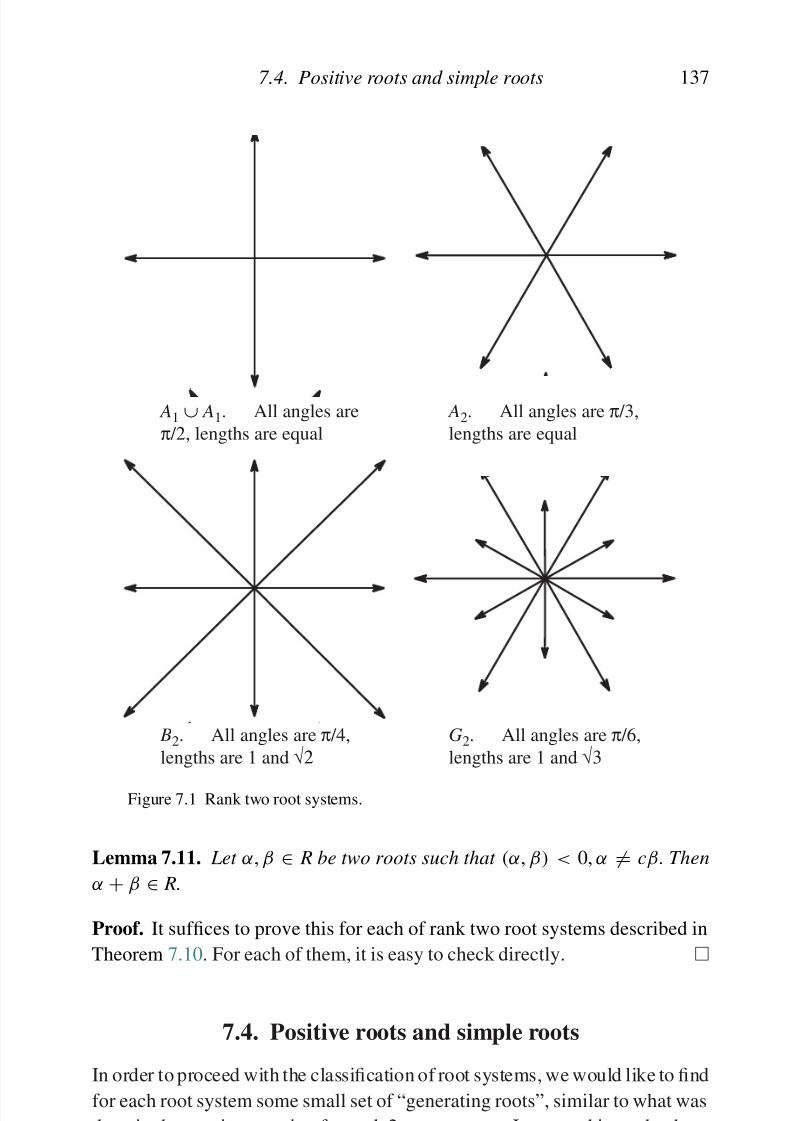
8/21/2019 Introduction to Lie Groups and Lie Algebras
http://slidepdf.com/reader/full/introduction-to-lie-groups-and-lie-algebras 149/236
7.4. Positive roots and simple roots 137
A1 ∪ A1. All angles are
π /2, lengths are equal
B2. All angles are π /4,
lengths are 1 and √2
G2. All angles are π /6,
lengths are 1 and √3
A2. All angles are π /3,
lengths are equal
Figure 7.1 Rank two root systems.
Lemma 7.11. Let α, β ∈ R be two roots such that (α, β) < 0, α = cβ. Then
α + β ∈ R.
Proof. It suffices to prove this for each of rank two root systems described in
Theorem 7.10. For each of them, it is easy to check directly.
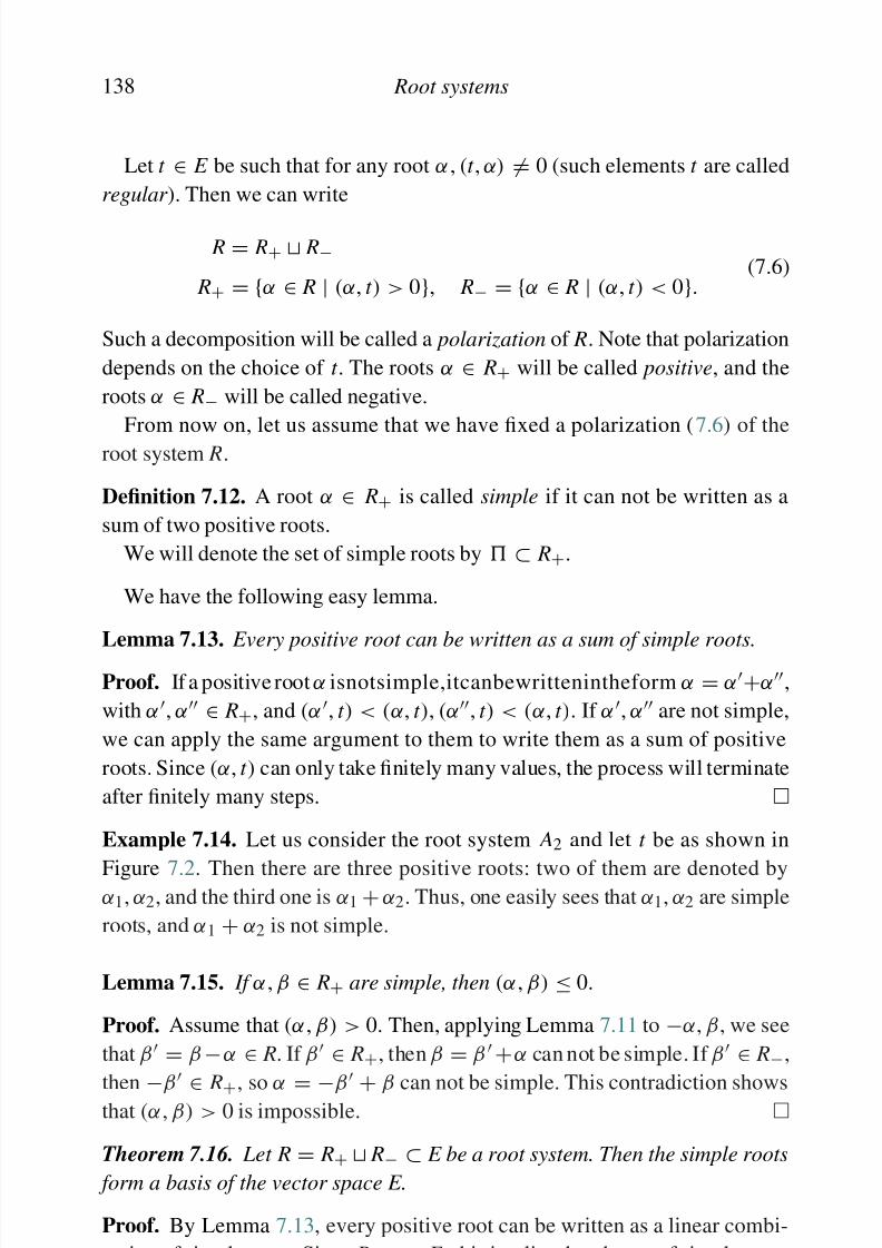
8/21/2019 Introduction to Lie Groups and Lie Algebras
http://slidepdf.com/reader/full/introduction-to-lie-groups-and-lie-algebras 150/236
138 Root systems
Let t ∈ E be such that for any root α , (t , α) = 0 (such elements t are called
regular ). Then we can write
R = R+ R− R+ = {α ∈ R | (α, t ) > 0}, R− = {α ∈ R | (α, t ) < 0}.
(7.6)
Such a decomposition will be called a polarization of R. Note that polarization
depends on the choice of t . The roots α ∈ R+ will be called positive, and the
roots α ∈ R− will be called negative.
From now on, let us assume that we have fixed a polarization (7.6) of the
root system R.
Definition 7.12. A root α ∈ R+ is called simple if it can not be written as a
sum of two positive roots.
We will denote the set of simple roots by ⊂ R+.
We have the following easy lemma.
Lemma 7.13. Every positive root can be written as a sum of simple roots.
Proof. If a positive root α isnotsimple,itcanbewrittenintheform α = α+α,with α , α ∈ R+, and (α , t ) < (α, t ), (α, t ) < (α, t ). If α , α are not simple,
we can apply the same argument to them to write them as a sum of positive
roots. Since (α, t ) can only take finitely many values, the process will terminate
after finitely many steps.
Example 7.14. Let us consider the root system A2 and let t be as shown in
Figure 7.2. Then there are three positive roots: two of them are denoted byα1, α2, and the third one is α1 + α2. Thus, one easily sees that α1, α2 are simple
roots, and α1 + α2 is not simple.
Lemma 7.15. If α , β ∈ R+ are simple, then (α , β) ≤ 0.
Proof. Assume that (α , β) > 0. Then, applying Lemma 7.11 to −α, β, we see
that β = β −α ∈ R. If β ∈ R+, then β = β +α can not be simple. If β ∈ R−,
then −β ∈ R+, so α = −β + β can not be simple. This contradiction showsthat (α , β) > 0 is impossible.
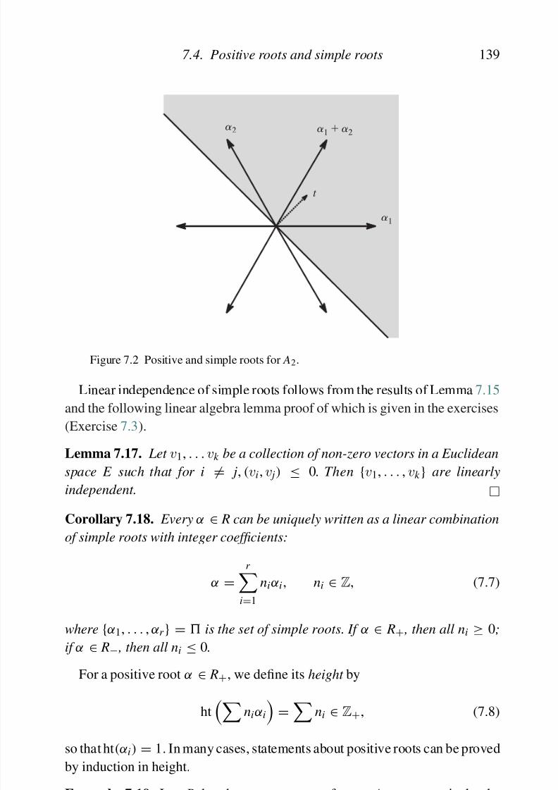
8/21/2019 Introduction to Lie Groups and Lie Algebras
http://slidepdf.com/reader/full/introduction-to-lie-groups-and-lie-algebras 151/236
7.4. Positive roots and simple roots 139
t
a2
a1
a1 a2
Figure 7.2 Positive and simple roots for A2.
Linear independence of simple roots follows from the results of Lemma 7.15
and the following linear algebra lemma proof of which is given in the exercises(Exercise 7.3).
Lemma 7.17. Let v1, . . . vk be a collection of non-zero vectors in a Euclidean
space E such that for i = j, (vi, v j) ≤ 0. Then {v1, . . . , vk } are linearly
independent.
Corollary 7.18. Every α ∈ R can be uniquely written as a linear combination
of simple roots with integer coefficients:
α =r
i=1
niαi, ni ∈ Z, (7.7)
where {α1, . . . , αr } = is the set of simple roots. If α ∈ R+ , then all ni ≥ 0;
if α ∈ R− , then all ni ≤ 0.
For a positive root α
∈ R+, we define its height by
ht
niαi
=
ni ∈ Z+, (7.8)

8/21/2019 Introduction to Lie Groups and Lie Algebras
http://slidepdf.com/reader/full/introduction-to-lie-groups-and-lie-algebras 152/236
140 Root systems
polarization as follows:
R+ = {ei − e j | i < j}
(the corresponding root subspaces E ij , i < j, generate the Lie subalgebra n of
strictly upper-triangular matrices in sl(n,C)).
Then it is easy to show that the simple roots are
α1 = e1 − e2, α2 = e2 − e3, . . . , αn−1 = en−1 − en,
and indeed, any positive root can be written as a sum of simple roots with non-
negative integer coefficients. For example, e2 − e4 = (e2 − e3) + (e3 − e4) =α2 + α3. The height is given by ht(ei − e j) = j − i.
7.5. Weight and root lattices
In the study of root systems of simple Lie algebras, we will frequently use thefollowing lattices. Recall that a lattice in a real vector space E is an abelian
group generated by a basis in E . Of course, by a suitable change of basis any
lattice L ⊂ E can be identified with Zn ⊂ Rn.
Every root system R ⊂ E gives rise to the following lattices:
Q = {abelian group generated by α ∈ R} ⊂ E
Q∨ = {abelian group generated by α∨, α ∈ R} ⊂ E ∗ (7.9)
Lattice Q is called the root lattice of R, and Q∨ is the coroot lattice. Note that
despite the notation, Q∨ is not the dual lattice to Q.
To justify the use of the word lattice, we need to show that Q, Q∨ are indeed
generated by a basis in E (respectively E ∗). This can be done as follows. Fix
a polarization of R and let = {α1, . . . , αr } be the corresponding system of
simple roots. Since every root can be written as a linear combination of simple
roots with integer coefficients (Corollary 7.18), one has
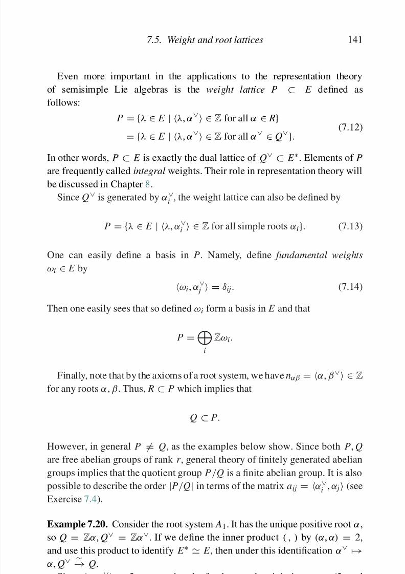
8/21/2019 Introduction to Lie Groups and Lie Algebras
http://slidepdf.com/reader/full/introduction-to-lie-groups-and-lie-algebras 153/236
7.5. Weight and root lattices 141
Even more important in the applications to the representation theory
of semisimple Lie algebras is the weight lattice P
⊂ E defined as
follows:
P = {λ ∈ E | λ, α∨ ∈ Z for all α ∈ R}= {λ ∈ E | λ, α∨ ∈ Z for all α∨ ∈ Q∨}.
(7.12)
In other words, P ⊂ E is exactly the dual lattice of Q∨ ⊂ E ∗. Elements of P
are frequently called integral weights. Their role in representation theory will
be discussed in Chapter 8.
Since Q∨ is generated by α∨i , the weight lattice can also be defined by
P = {λ ∈ E | λ, α∨i ∈ Z for all simple roots αi}. (7.13)
One can easily define a basis in P. Namely, define fundamental weights
ωi ∈ E by
ωi, α∨ j = δij. (7.14)
Then one easily sees that so defined ωi form a basis in E and that
P =
i
Zωi.
Finally, note that by the axioms of a root system, we have nαβ = α, β∨ ∈ Zfor any roots α, β. Thus, R ⊂ P which implies that
Q ⊂ P.
However, in general P = Q, as the examples below show. Since both P, Q
are free abelian groups of rank r , general theory of finitely generated abelian
groups implies that the quotient group P/Q is a finite abelian group. It is also
possible to describe the order |P/Q| in terms of the matrix aij = α∨i , α j (see
Exercise 7.4).
E l 7 20 C id h A I h h i i i
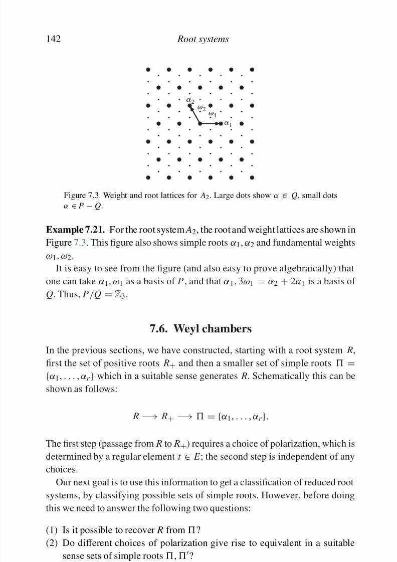
8/21/2019 Introduction to Lie Groups and Lie Algebras
http://slidepdf.com/reader/full/introduction-to-lie-groups-and-lie-algebras 154/236
142 Root systems
a2
a1
v1
v2
Figure 7.3 Weight and root lattices for A2. Large dots show α ∈ Q, small dotsα ∈ P − Q.
Example 7.21. For the root system A2, the root and weight lattices are shown in
Figure 7.3. This figure also shows simple roots α1, α2 and fundamental weights
ω1, ω2.
It is easy to see from the figure (and also easy to prove algebraically) that
one can take α1, ω1 as a basis of P , and that α1, 3ω1 = α2 + 2α1 is a basis of
Q. Thus, P/Q = Z3.
7.6. Weyl chambers
In the previous sections, we have constructed, starting with a root system R,
first the set of positive roots R+ and then a smaller set of simple roots ={α1, . . . , αr } which in a suitable sense generates R. Schematically this can be
shown as follows:
R −→ R+ −→ = {α1, . . . , αr }.
The first step (passage from R to R+) requires a choice of polarization, which is
determined by a regular element t ∈ E ; the second step is independent of any
choices.
Our next goal is to use this information to get a classification of reduced root
systems, by classifying possible sets of simple roots. However, before doing
this we need to answer the following two questions:
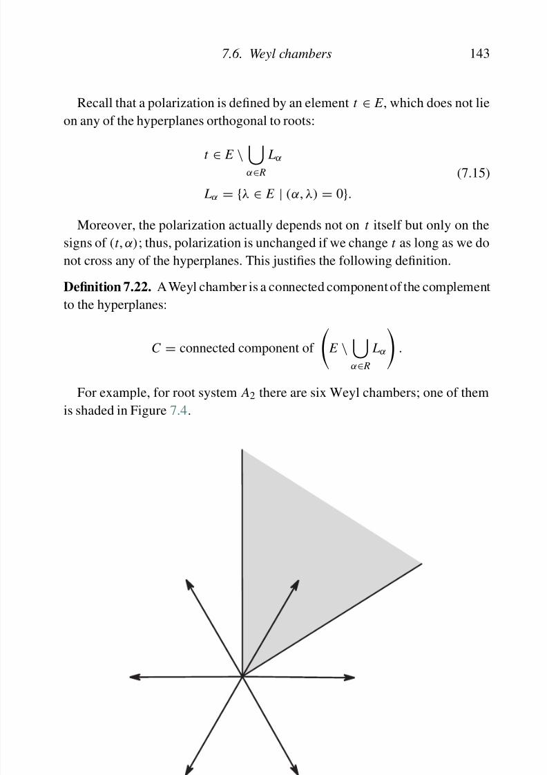
8/21/2019 Introduction to Lie Groups and Lie Algebras
http://slidepdf.com/reader/full/introduction-to-lie-groups-and-lie-algebras 155/236
7.6. Weyl chambers 143
Recall that a polarization is defined by an element t ∈ E , which does not lie
on any of the hyperplanes orthogonal to roots:
t ∈ E \α∈ R
Lα
Lα = {λ ∈ E | (α, λ) = 0}.
(7.15)
Moreover, the polarization actually depends not on t itself but only on the
signs of (t , α); thus, polarization is unchanged if we change t as long as we do
not cross any of the hyperplanes. This justifies the following definition.
Definition 7.22. A Weyl chamber is a connected component of the complement
to the hyperplanes:
C = connected component of
E \
α∈ R
Lα
.
For example, for root system A2 there are six Weyl chambers; one of them
is shaded in Figure 7.4.
8/21/2019 Introduction to Lie Groups and Lie Algebras
http://slidepdf.com/reader/full/introduction-to-lie-groups-and-lie-algebras 156/236
144 Root systems
Clearly, to specify a Weyl chamber we need to specify, for each hyperplane
Lα, on which side of the hyperplane the Weyl chamber lies. Thus, a Weyl
chamber is defined by a system of inequalities of the form
±(α, λ) > 0
(one inequality for each root hyperplane). Any such system of inequalities
defines either an empty set or a Weyl chamber.
For future use, we state here some results about the geometry of the Weyl
chambers.
Lemma 7.23.
(1) The closure C of a Weyl chamber C is an unbounded convex cone.
(2) The boundary ∂C is a union of finite number of codimension one faces:
∂C = F i. Each F i is a closed convex unbounded subset in one of
the hyperplanes Lα , given by a system of inequalities. The hyperplanes
containing F i are called walls of C.
This lemma is geometrically obvious (in fact, it equally applies to any subset
in a Euclidean space defined by a finite system of strict inequalities) and we
omit the proof.
We can now return to the polarizations. Note that anyWeyl chamber C defines
a polarization given by
R+ = {α ∈ R | (α, t ) > 0}, t ∈ C (7.16)
(this does not depend on the choice of t ∈ C ). Conversely, given a polarization
R = R+ R−, define the corresponding positive Weyl chamber C + by
C + = {λ ∈ E | (λ, α) > 0 for all α ∈ R+}= {λ ∈ E | (λ, αi) > 0 for all αi ∈ }
(7.17)
(to prove the last equality, note that if (λ, αi) > 0 for all αi
∈ , then by
Lemma 7.13, for any α = niαi, we have (λ, α) > 0). This system of inequal-
ities does have solutions (because the element t used to define the polarization
8/21/2019 Introduction to Lie Groups and Lie Algebras
http://slidepdf.com/reader/full/introduction-to-lie-groups-and-lie-algebras 157/236
7.6. Weyl chambers 145
In order to relate polarizations defined by different Weyl chambers, recall
the Weyl group W defined in Section 7.2 Since the action of W maps root
hyperplanes to root hyperplanes, we have a well-defined action of W on the set
of Weyl chambers.
Theorem 7.25. The Weyl group acts transitively on the set of Weyl chambers.
Proof. The proof is based on several facts which are of significant interest in
their own right. Namely, let us say that two Weyl chambers C , C are adjacent
if they have a common codimension one face F (obviously, they have to be on
different sides of F ). If Lα is the hyperplane containing this common face F ,then we will say that C , C are adjacent chambers separated by Lα .
Then we have the following two lemmas, proof of which as an exercise to
the reader.
Lemma 7.26. Any two Weyl chambers C , C can be connected by a sequence
of chambers C 0 = C , C 1, . . . , C l = C such that C i is adjacent to C i+1.
Lemma 7.27. If C , C are adjacent Weyl chambers separated by hyperplane Lα then sα(C ) = C .
The statement of the theorem now easily follows from these two lemmas.
Indeed, let C , C be two Weyl chambers. By Lemma 7.26, they can be connected
by a sequence of Weyl chambers C 0 = C , C 1, . . . , C l = C . Let Lβi be the
hyperplane separating C i−1 and C i. Then, by Lemma 7.27,
C l = sβl (C l−1) = sβl sβl−1 (C l−2) = . . .= sβl
. . . sβ1(C 0)
(7.18)
so C = w(C ), with w = sβl . . . sβ1
. This completes the proof of Theorem 7.25.
Corollary 7.28. Every Weyl chamber has exactly r = rank ( R) walls. Walls of
positive Weyl chamber C
+ are Lαi
, αi
∈ .
Proof. For the positive Weyl chamber C +, this follows from (7.17). Since every
8/21/2019 Introduction to Lie Groups and Lie Algebras
http://slidepdf.com/reader/full/introduction-to-lie-groups-and-lie-algebras 158/236
146 Root systems
Proof. By Lemma 7.24, each polarization is defined by a Weyl chamber. Since
W acts transitively on the set of Weyl chambers, it also acts transitively on the
set of all polarizations.
This last corollary provides an answer to the question asked in the beginning
of this section: sets of simple roots obtained from different polarizations can be
related by an orthogonal transformation of E .
7.7. Simple reflections
We can now return to the first question asked in the beginning of the previous
section: is it possible to recover R from the set of simple roots ? The answer
is again based on the use of Weyl group.
Theorem 7.30. Let R be a reduced root system, with fixed polarization R = R+ R−. Let = {α1, . . . , αr } be the set of simple roots. Consider reflections
corresponding to simple roots si = sαi (they are called simple reflections).
(1) The simple reflections si generate W .
(2) W () = R: every α ∈ R can be written in the form w(αi) for some w ∈ W
and αi ∈ .
Proof. We start by proving the following result
Lemma 7.31. Any Weyl chamber can be written as
C = si1 . . . sil
(C +)
for some sequence of indices i1, . . . , il ∈ {1, . . . , r }. ( Here C + is the positive
Weyl chamber defined by (7.17).)
Proof. By the construction given in the proof of Theorem 7.25, we can connect
C +, C by a chain of adjacent Weyl chambers C 0 = C +, C 1, . . . , C l = C . Then
C = sβl . . . sβ1 (C +), where Lβi is the hyperplane separating C i−1 and C i.Since Lβ1
separates C 0 = C + from C 1, it means that Lβ1 is one of the walls of
C Si h ll f C l h l L di i l

8/21/2019 Introduction to Lie Groups and Lie Algebras
http://slidepdf.com/reader/full/introduction-to-lie-groups-and-lie-algebras 159/236
7.7. Simple reflections 147
By Lemma 7.7, we therefore have sβ2 = si1
si2si1
and thus
sβ2 sβ1 = si1 si2 si1 · si1 = si1 si2
C 2 = si1si2
(C +).
Repeating the same argument, we finally get that
C = si1 . . . sil
(C +)
and the indices ik are computed inductively, by
βk = si1 . . . sik −1
(αik ) (7.19)
which completes the proof of the lemma.
Now the theorem easily follows. Indeed, every hyperplane Lα is a wall of
some Weyl chamber C . Using the lemma, we can write C = w(C +) for some
w
= si
1
. . . sil
. Thus, Lα
= w( Lα
j
) for some index j, so α
= ±w(α j) and
sα = ws jw−1, which proves both statements of the theorem.
It is also possible to write the full set of defining relations for W (see
Exercise 7.11).
Example 7.32. Let R be the root system of type An−1. Then the Weyl group
is W = S n (see Example 7.8) and simple reflections are transpositions si =(i i + 1). And indeed, it is well known that these transpositions generate the
symmetric group.We can also describe the Weyl chambers in this case. Namely, the positive
Weyl chamber is
C + = {(λ1, . . . , λn) ∈ E | λ1 ≥ λ2 ≥ · · · ≥ λn}
and all other Weyl chambers are obtained by applying to C + permutations
σ
∈ S n. Thus, they are of the form
Cσ = {(λ1, . . . , λn) ∈ E | λσ (1) ≥ λσ (2) ≥ · · · ≥ λσ (n)}, σ ∈ Sn.
8/21/2019 Introduction to Lie Groups and Lie Algebras
http://slidepdf.com/reader/full/introduction-to-lie-groups-and-lie-algebras 160/236
148 Root systems
Let us say that a root hyperplane Lα separates two Weyl chambers C , C if
these two chambers are on different sides of Lα, i.e. α(C ), α(C ) have different
signs (we do not assume that Lα is one of the walls of C or C ).
Definition 7.34. Let R be a reduced root system, with the set of simple roots
. Then we define, for an element w ∈ W , its length by
l(w) = number of root hyperplanes separating C + and w(C +)
= |{α ∈ R+ | w(α) ∈ R−}|.(7.20)
It should be noted that l(w) depends not only on w itself but also on the
choice of polarization R = R+ R− or equivalently, the set of simple roots.
Example 7.35. Let w = si be a simple reflection. Then the Weyl chambers C +and si(C +) are separated by exactly one hyperplane, namely Lαi
. Therefore,
l(si) = 1, and
{α ∈ R+ | si(α) ∈ R−} = {αi}. (7.21)
In other words, si(αi) = −αi ∈ R− and si permutes elements of R+ \ {αi}.
This example is very useful in many arguments involving Weyl group, such
as the following lemma.
Lemma 7.36. Let
ρ = 1
2
α∈ R+
α. (7.22)
Then
ρ, α∨i =
2(ρ, αi)/(α
i, α
i) =
1.
Proof. Writing ρ = (αi +
α∈ R+\{αi} α)/2 and using results of Example 7.35,
we see that si(ρ) = ρ − αi. On the other hand, by definition si(λ) = λ −α∨
i , λαi.
Theorem 7.37. Let
w = si1 . . . sil
be an expression for w as a product of simple reflections which has minimal possible length (such expressions are called reduced). Then l = l(w).
8/21/2019 Introduction to Lie Groups and Lie Algebras
http://slidepdf.com/reader/full/introduction-to-lie-groups-and-lie-algebras 161/236
7.8. Dynkin diagrams and classification of root systems 149
hyperplanes. In particular, this means that C + and w(C +) are separated by at
most l hyperplanes, so l (w)
≤ l.
Note, however, that we can not yet conclude that l(w) = l: it is possible
that the path we had constructed crosses some hyperplane more than once. For
example, we can write 1 = sisi, which gives us a path connecting C + with itself
but crossing hyperplane Lαi twice. So to show that l (w) = l, we need to show
that if w = si1 . . . sil
is a reduced expression, then all hyperplanes Lβ1, . . . , Lβl
are distinct: we never cross any hyperplane more than once. The proof of this
fact is given as an exercise (see Exercise 7.6).
Corollary 7.38. The action of W on the set of Weyl chambers is simply
transitive.
Proof. Otherwise, there exists w ∈ W such that w(C +) = C +. By definition,
this means l (w) = 0. By Theorem 7.37, this implies that w = 1.
This shows that C + is the fundamental domain for the action of W on E . In
fact, we have a stronger result: every W -orbit in E contains exactly one element
from C + (see Exercise 7.8).
Lemma 7.39. Let C − be the negative Weyl chamber: C − = −C + and let
w0 ∈ W be such that w0(C +) = C − (by Corollary 7.38 , such an element exists
and is unique). Then l(w0) = | R+| and for any w ∈ W , w = w0 , we have
l(w) < l(w0). For this reason w0 is called the longest element in W .
The proof of this lemma is left to the reader as an exercise.
7.8. Dynkin diagrams and classification of root systems
In the previous sections, we have discussed that given a reduced root system
R, we can choose a polarization R = R+ R− and then define the set of
simple roots = {α1, . . . , αr }. We have shown that R can be recovered from
(Corollary 7.33) and that different choices of polarization give rise to sets of
simple roots which are related by the action of the Weyl group (Corollary 7.29).Thus, classifying root systems is equivalent to classifying possible sets of simple
8/21/2019 Introduction to Lie Groups and Lie Algebras
http://slidepdf.com/reader/full/introduction-to-lie-groups-and-lie-algebras 162/236
150 Root systems
on E 1 ⊕ E 2 defined so that E 1 ⊥ E 2. It is easy to see that so defined R is again
a root system.
Definition 7.40. A root system R is called reducible if it can be written in the
form R = R1 R2, with R1 ⊥ R2. Otherwise, R is called irreducible.
For example, the root system A1 ∪ A1 discussed in Section 7.3 is reducible;
all other root systems discussed in that section are irreducible.
Remark 7.41. It should be noted that a root system being reducible or irre-
ducible is completely unrelated to whether the root system is reduced or
not. It would be best if a different terminology were used, to avoid confu-
sion; however, both of these terms are so widely used that changing them is
not feasible.
There is an analogous notion for the set of simple roots.
Lemma 7.42. Let R be a reduced root system, with given polarization, and let
be the set of simple roots.
(1) If R is reducible: R = R1 R2 , then = 1 2 , where i = ∩ Ri is
the set of simple roots for Ri.
(2) Conversely, if = 1 2 , with 1 ⊥ 2 , then R = R1 R2 , where Ri
is the root system generated by i.
Proof. The first part is obvious. To prove the second part, notice that if α
∈1, β ∈ 2, then sα(β) = β and sα, sβ commute. Thus, if we denote by W i
the group generated by simple reflections sα, α ∈ i, then W = W 1 × W 2, and
W 1 acts trivially on 2, W 2 acts trivially on 1. Thus, R = W (1 2) =W 1(1) W 2(2).
It can be shown that every reducible root system can be uniquely written in
the form R1 R2 · · · Rn, where Ri are mutually orthogonal irreducible root
systems. Thus, in order to classify all root systems, it suffices to classify allirreducible root systems. For this reason, from now on R is an irreducible root
d i h di f i l W h h
8/21/2019 Introduction to Lie Groups and Lie Algebras
http://slidepdf.com/reader/full/introduction-to-lie-groups-and-lie-algebras 163/236
7.8. Dynkin diagrams and classification of root systems 151
Definition 7.43. The Cartan matrix A of a set of simple roots ⊂ R is the
r
×r matrix with entries
aij = nα j αi = α∨
i , α j = 2(αi, α j)
(αi, αi). (7.23)
The following properties of the Cartan matrix immediately follow from the
definitions and from known properties of simple roots.
Lemma 7.44.
(1) For any i, aii = 2.(2) For any i = j, aij is a non-positive integer: aij ∈ Z, aij ≤ 0.
(3) For any i = j, aija ji = 4cos2 ϕ, where ϕ is the angle between αi, α j. If
ϕ = π/2, then
|αi|2
|α j|2 = a ji
aij
.
Example 7.45. For the root system An, the Cartan matrix is
A =
2 −1
−1 2 −1
−1 2 −1...
−1 2 −1
−1 2
(entries which are not shown are zeroes).
The information contained in the Cartan matrix can also be presented in a
graphical way.
Definition 7.46. Let be a set of simple roots of a root system R. The Dynkin
diagram of is the graph constructed in the following manner.
• For each simple root αi, we construct a vertex v
i of the Dynkin diagram(traditionally, vertices are drawn as small circles rather than as dots).
F h i f i l h di i
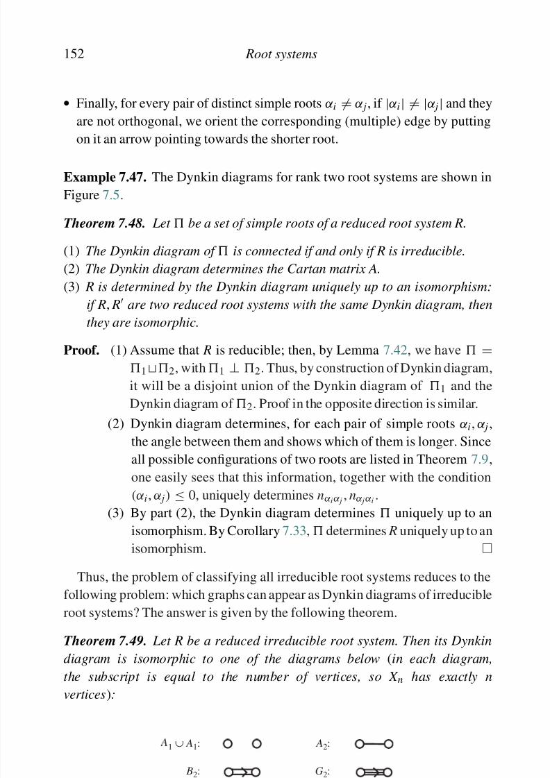
8/21/2019 Introduction to Lie Groups and Lie Algebras
http://slidepdf.com/reader/full/introduction-to-lie-groups-and-lie-algebras 164/236
152 Root systems
• Finally, for every pair of distinct simple roots αi = α j, if |αi| = |α j| and they
are not orthogonal, we orient the corresponding (multiple) edge by putting
on it an arrow pointing towards the shorter root.
Example 7.47. The Dynkin diagrams for rank two root systems are shown in
Figure 7.5.
Theorem 7.48. Let be a set of simple roots of a reduced root system R.
(1) The Dynkin diagram of is connected if and only if R is irreducible.
(2) The Dynkin diagram determines the Cartan matrix A.(3) R is determined by the Dynkin diagram uniquely up to an isomorphism:
if R, R are two reduced root systems with the same Dynkin diagram, then
they are isomorphic.
Proof. (1) Assume that R is reducible; then, by Lemma 7.42, we have =1 2, with 1 ⊥ 2. Thus, by construction of Dynkin diagram,
it will be a disjoint union of the Dynkin diagram of 1 and the
Dynkin diagram of 2. Proof in the opposite direction is similar.(2) Dynkin diagram determines, for each pair of simple roots αi, α j ,
the angle between them and shows which of them is longer. Since
all possible configurations of two roots are listed in Theorem 7.9,
one easily sees that this information, together with the condition
(αi, α j) ≤ 0, uniquely determines nαi α j, nα j αi
.
(3) By part (2), the Dynkin diagram determines uniquely up to an
isomorphism. By Corollary 7.33, determines R uniquely up to an
isomorphism.
Thus, the problem of classifying all irreducible root systems reduces to the
following problem: which graphs can appear as Dynkin diagrams of irreducible
root systems? The answer is given by the following theorem.
Theorem 7.49. Let R be a reduced irreducible root system. Then its Dynkin
diagram is isomorphic to one of the diagrams below (in each diagram,
the subscript is equal to the number of vertices, so X n has exactly nvertices):
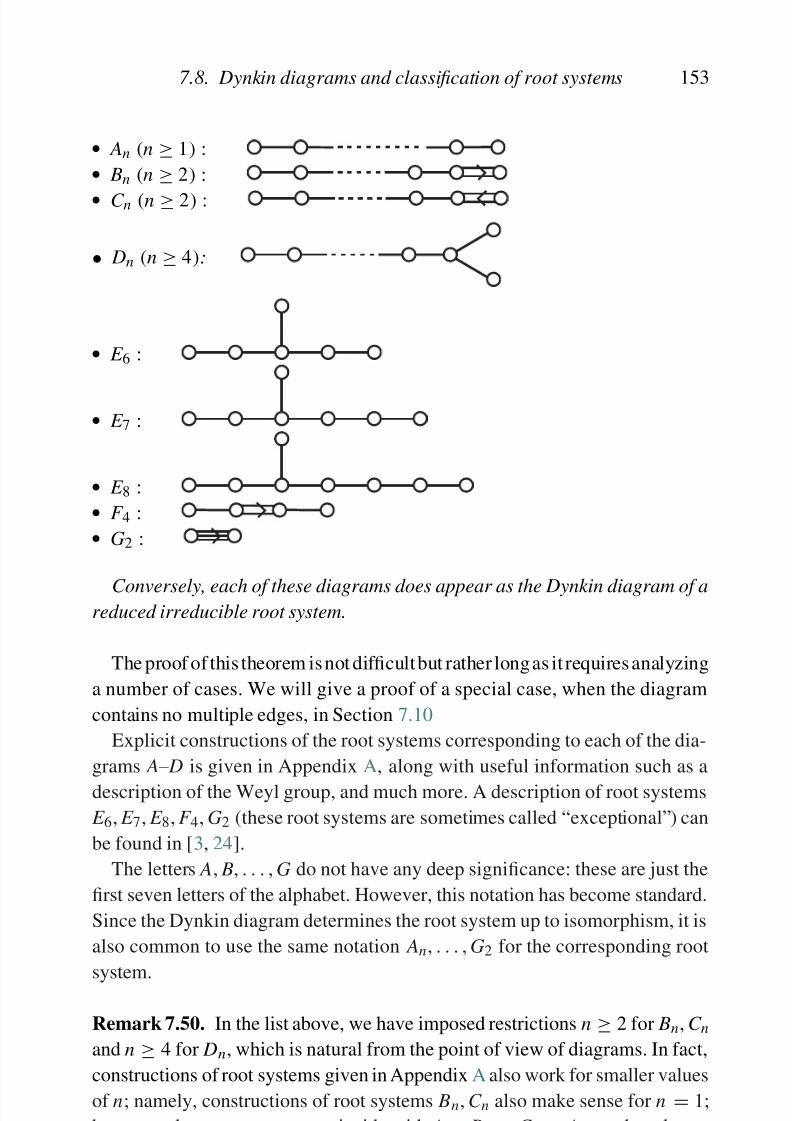
8/21/2019 Introduction to Lie Groups and Lie Algebras
http://slidepdf.com/reader/full/introduction-to-lie-groups-and-lie-algebras 165/236
7.8. Dynkin diagrams and classification of root systems 153
• An (n ≥ 1) :
• Bn (n
≥ 2) :
• C n (n ≥ 2) :
• Dn (n ≥ 4):
• E 6 :
• E 7 :
• E 8 :
• F 4 :
• G2 :
Conversely, each of these diagrams does appear as the Dynkin diagram of areduced irreducible root system.
The proof of this theorem is not difficult but rather long as it requires analyzing
a number of cases. We will give a proof of a special case, when the diagram
contains no multiple edges, in Section 7.10
Explicit constructions of the root systems corresponding to each of the dia-
grams A– D is given in Appendix A, along with useful information such as a
description of the Weyl group, and much more. A description of root systems
E 6, E 7, E 8, F 4, G2 (these root systems are sometimes called “exceptional”) can
be found in [3, 24].
The letters A, B, . . . , G do not have any deep significance: these are just the
first seven letters of the alphabet. However, this notation has become standard.
Since the Dynkin diagram determines the root system up to isomorphism, it is
also common to use the same notation An, . . . , G2 for the corresponding root
system.
R k 7 50 I h li b h i d i i 2 f B C

8/21/2019 Introduction to Lie Groups and Lie Algebras
http://slidepdf.com/reader/full/introduction-to-lie-groups-and-lie-algebras 166/236
154 Root systems
to Lie algebra isomorphisms sl(2,C) so(3,C) sp(1,C) constructed in
Section 3.10 and sp(2,C)
so(5,C).)
Similarly, construction of the root system Dn also makes sense for n = 2, 3,
in which case it gives D2 = A1 ∪ A1, D3 = A3, which correspond to Lie
algebra isomorphisms so(4,C) sl(2,C) ⊕ sl(2,C), so(6,C) sl(4,C), see
Exercise 6.6.
Other than the equalities listed above, all root systems An, . . . , G2 are
distinct.
Corollary 7.51. If R is a reduced irreducible root system, then (α, α) can take
at most two different values. The number
m = max(α, α)
min(α, α)(7.24)
is equal to the maximal multiplicity of an edge in the Dynkin diagram; thus,
m = 1 for root systems of types ADE (these are called simply-laced diagrams) ,
m = 2 for types BCF, and m = 3 for G2.
For non-simply laced systems, the roots with (α, α) being the larger of two possible values are called the long roots , and the remaining roots are called
short.
7.9. Serre relations and classification of semisimple
Lie algebras
We can now return to the question of classification of complex semisimple Liealgebras. Since every semisimple algebra is a direct sum of simple ones, it
suffices to classify simple Lie algebras.
According to the results of Section 6.6, every semisimple Lie algebra defines
a reduced root system; if the algebra is not simple but only semisimple, then
the root system is reducible. The one question we have not yet answered is
whether one can go back and recover the Lie algebra from the root system. If
the answer is positive, then the isomorphism classes of simple Lie algebras are
in bijection with the isomorphism classes of reduced irreducible root systems,and thus we could use classification results of Section 7.8 to classify simple
8/21/2019 Introduction to Lie Groups and Lie Algebras
http://slidepdf.com/reader/full/introduction-to-lie-groups-and-lie-algebras 167/236
7.9. Serre relations and classification of semisimple Lie algebras 155
(1) The subspaces
n
± = α∈ R±
gα (7.25)
are subalgebras in g , and
g = n− ⊕ h ⊕ n+ (7.26)
as a vector space.
(2) Let ei ∈ gαi, f i ∈ g−αi
be chosen so that (ei, f i) = 2/(αi, αi) , and let
hi = hαi ∈ h be defined by (6.5). Then e1, . . . , er generate n+, f 1, . . . , f r generate n− , and h1, . . . , hr form a basis of h. In particular, {ei, f i, hi}i=1...r
generate g.
(3) The elements ei, f i, hi satisfy the following relations, called the Serre
relations:
[hi, h j] = 0 (7.27)
[hi, e j
] = aije j,
[hi, f j
] = −aij f j (7.28)
[ei, f j] = δijhi (7.29)
(ad ei)1−aij e j = 0 (7.30)
(ad f i)1−aij f j = 0 (7.31)
where aij = nα j ,αi = α∨
i , α j are the entries of the Cartan matrix.
Proof.
(1) The fact that n+ is a subalgebra follows from [gα, gβ] ⊂ gα+β (see Theo-
rem 6.38) and the fact that the sum of positive roots is positive. Equation
(7.26) is obvious.
(2) The fact that hi form a basis of h follows from Theorem 7.16. To prove that
ei generate n+, we first prove the following lemma.
Lemma 7.53. Let R
= R
+ R
− be a reduced root system, with a set of
simple roots {α1, . . . , αr }. Let α be a positive root which is not simple. Thenα = β + αi for some positive root β and simple root αi.
8/21/2019 Introduction to Lie Groups and Lie Algebras
http://slidepdf.com/reader/full/introduction-to-lie-groups-and-lie-algebras 168/236
156 Root systems
to check that β must be a positive root. This completes the proof of
the lemma.
By Theorem 6.44, under the assumption of the lemma we have
gα = [gβ , ei]. Using induction in height ht(α) (see equation (7.8)), it is
now easy to show that ei generate n+. Similar argument shows that f i
generate n−.
(3) Relations (7.27), (7.28) are an immediate corollary of the definition of Car-
tan subalgebra and root subspace. Commutation relation [ei, f i] = hi is part
of Lemma 6.42 (about sl(2,C)-triple determined by a root). Commutation
relation [ei, f j] = 0 for i = j follows from the fact that [ei, f j] ∈ gαi−α j.
But αi −α j is not a root (it can not be a positive root because the coefficient
of α j is negative, and it can not be a negative root because the coefficient
of αi is positive). Thus, [ei, f j] = 0.
To prove relations (7.31), consider the subspace
k ∈Z gα j+k αi ⊂ g as
a module over sl(2,C) triple generated by ei, f i, hi. Since ad ei. f j = 0, f j
is a highest-weight vector; by (7.29), its weight is equal to −aij . Results
of Section 4.8 about representation theory of sl(2,C), imply that if v is avector of weight λ in a finite-dimensional representation, with e.v = 0,
then f λ+1.v = 0. Applying it to f j, we get (7.31). Equality (7.30) is proved
similarly.
This completes the proof of Theorem 7.52.
A natural question is whether (7.27) – (7.31) is a full set of defining relations
for g. The answer is given by the following theorem.
Theorem 7.54. Let R be a reduced irreducible root system, with a polarization
R = R+ R− and system of simple roots = {α1, . . . , αr }. Let g( R) be
the complex Lie algebra with generators ei, f i, hi, i = 1 . . . , r and relations
(7.27) – (7.31). Then g is a finite-dimensional semisimple Lie algebra with root
system R.
The proof of this theorem is not given here; interested reader can find it in
[47], [22], or [24]. We note only that it is highly non-trivial that g( R) is finite-dimensional (in fact, this is the key step of the proof), which in turn is based on
8/21/2019 Introduction to Lie Groups and Lie Algebras
http://slidepdf.com/reader/full/introduction-to-lie-groups-and-lie-algebras 169/236
7.10. Proof of the classification theorem in simply-laced case 157
(2) There is a natural bijection between the set of isomorphism classes
of reduced root systems and the set of isomorphism classes of finite-
dimensional complex semisimple Lie algebras. The Lie algebra is simple
iff the root system is irreducible.
Combining this corollary with the classification given in Theorem 7.49, we
get the following celebrated result.
Theorem 7.56. Simple finite-dimensional complex Lie algebras are classified
by Dynkin diagrams An . . . G2 listed in Theorem 7.49.
It is common to refer to the simple Lie algebra corresponding to the Dynkin
diagram, say, E 6, as “simple Lie algebra of type E 6”.
It is possible to give an explicit construction of the simple Lie algebra corre-
sponding to each of the Dynkin diagrams of Theorem 7.49. For example, Lie
algebra of type An is nothing but sl(n + 1,C). Series Bn, C n, Dn correspond
to classical Lie algebras so and sp. These root systems and Lie algebras are
described in detail in Appendix A. Construction of exceptional Lie algebras, of types E 6, E 7, E 8, F 4, G2, can be found in [3] or in [24].
7.10. Proof of the classification theorem in
simply-laced case
In this section, we give a proof of the classification theorem for Dynkin
diagrams (Theorem 7.49) in a special case when the diagram is simply-laced,
i.e. contains no multiple edges. This section can be skipped at the first
reading.
Let D be a connected simply-laced Dynkin diagram, with the set of vertices
I . Then all roots αi have the same length; without loss of generality, we can
assume that (αi, αi) = 2. Then the Cartan matrix is given by aij = (αi, α j). In
particular, this implies the following important rule.
For any J ⊂ I the matrix (aij)i j∈J is positive definite (7 32)

8/21/2019 Introduction to Lie Groups and Lie Algebras
http://slidepdf.com/reader/full/introduction-to-lie-groups-and-lie-algebras 170/236
158 Root systems
Step 1. D contains no cycles.
Indeed, otherwise D contains a subdiagram which is a cycle. But for such a
subdiagram, bilinear form defined by the Cartan matrix is not positive definite:
explicit computation shows that vector
j∈ J α j is in the kernel of this form.
Step 2. Each vertex is connected to at most three others.
Indeed, otherwise D would contain the subdiagram shown in Figure 7.6. For
such a subdiagram, however, the bilinear form defined by the Cartan matrix is
not positive definite: vector 2α + (β1 + β2 + β3 + β4) is in the kernel of this
form.
Step 3. D contains at most one branching point (i.e., a vertex of valency more
than 2).
Indeed, otherwise D contains the subdiagram shown in Figure 7.7.
Let α = α1 + · · · + · · · αn. It is easy to see that α , β1, β2, β3, β4 are linearly
independent and thus the matrix of their inner products must be positive definite.
On the other hand, explicit computation shows that (α, α) = 2, (α, βi) = −1,
so the inner products between these vectors are given by the same matrix as in
Step 2 and which, as was shown above, is not positive definite.
Combining the three steps, we see that D must be either a chain, i.e.a diagram of type An, or a “star” diagram with three branches as shown
in Figure 7.8. Denote by p, q, r the lengths of these branches (including
the central vertex); for example, for diagram E 7 the lengths would be
2, 3, 4. Denote the roots corresponding to the branches of the diagram by
β1, . . . , β p−1, γ 1, . . . , γ q−1, δ1, . . . , δr −1 as shown in Figure 7.8.
Let α be the central vertex and let β =
p−1i=1 iβi, γ =
q−1i=1 iγ i, δ =
r −1
i=1
iδi. Then β, γ , δ are orthogonal, and vectors α, β, γ , δ are linearly
b1
b3 b4
b2
a
Figure 7.6
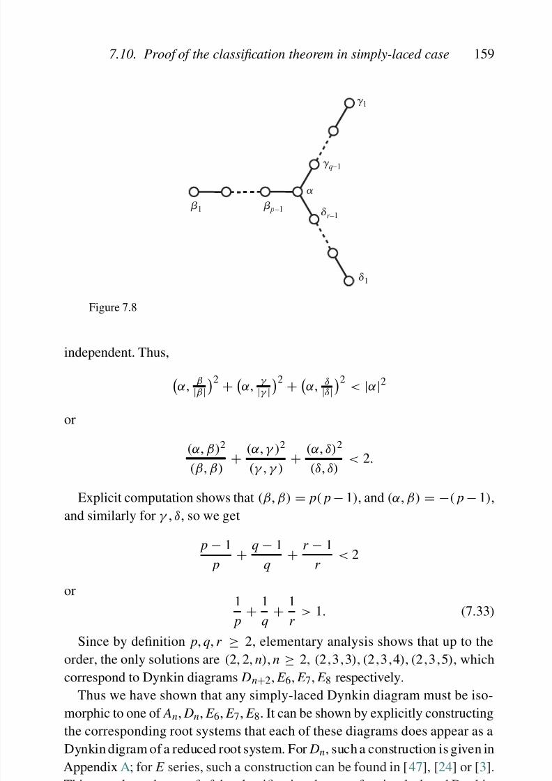
8/21/2019 Introduction to Lie Groups and Lie Algebras
http://slidepdf.com/reader/full/introduction-to-lie-groups-and-lie-algebras 171/236
7.10. Proof of the classification theorem in simply-laced case 159
b1
a
g 1
b p–1
g q–1
dr –1
d1
Figure 7.8
independent. Thus,
α,
β|β|
2 +
α,
γ |γ |
2 +
α, δ
|δ|2
< |α|2
or
(α, β)2
(β, β)+ (α, γ )2
(γ , γ )+ (α, δ)2
(δ, δ)< 2.
Explicit computation shows that (β, β) = p( p − 1), and (α, β) = −( p − 1),
and similarly for γ , δ, so we get
p − 1 p
+ q − 1q
+ r − 1r
< 2
or1
p+ 1
q+ 1
r > 1. (7.33)
Since by definition p, q, r ≥ 2, elementary analysis shows that up to the
order, the only solutions are (2, 2, n), n ≥ 2, (2,3,3), (2,3,4), (2,3,5), which
correspond to Dynkin diagrams Dn+2, E 6, E 7, E 8 respectively.Thus we have shown that any simply-laced Dynkin diagram must be iso-
hi f A D E E E I b h b li i l i
8/21/2019 Introduction to Lie Groups and Lie Algebras
http://slidepdf.com/reader/full/introduction-to-lie-groups-and-lie-algebras 172/236
160 Root systems
The proof for the non-simply-laced case is quite similar but requires a couple
of extra steps. This proof can be found in [22], [24], or [3] and will not be
repeated here.
7.11. Exercises
7.1. Let R ⊂ Rn be given by
R = {±ei, ±2ei | 1 ≤ i ≤ n}∪ {±ei ± e j | 1 ≤ i, j ≤ n, i = j},
where ei is the standard basis in Rn. Show that R is a non-reduced root
system. (This root system is usually denoted BC n.)
7.2. (1) Let R ⊂ E be a root system. Show that the set
R∨ = {α∨ | α ∈ R} ⊂ E ∗,
where α∨
∈ E ∗ is the coroot defined by (7.4), is also a root system.
It is usually called the dual root system of R.
(2) Let = {α1, . . . , αr } ⊂ R be the set of simple roots. Show that the
set ∨ = {α∨1 , . . . , α∨
r } ⊂ R∨ is the set of simple roots of R∨. [Note:
this is not completely trivial, as α → α∨ is not a linear map. Try
using equation (7.17).]
7.3. Prove Lemma 7.17. (Hint: any linear dependence can be written in the
form i∈ I
civi = j∈ J
c jv j,
where I ∩ J = ∅, ci, c j ≥ 0. Show that if one denotes v = i∈ I civi,
then (v, v) ≤ 0. )
7.4. Show that |P/Q| = | det A|, where A is the Cartan matrix: aij = α∨i , α j.
7.5. Compute explicitly the group P/Q for root systems An, Dn. 4
7 6 C l h i h f f Th 7 37 N l h

8/21/2019 Introduction to Lie Groups and Lie Algebras
http://slidepdf.com/reader/full/introduction-to-lie-groups-and-lie-algebras 173/236
7.11. Exercises 161
7.7. Let w = si1 . . . sil
be a reduced expression. Show that then
{α ∈ R+ | w(α) ∈ R−} = {β1, . . . , βl}
where βk = si1 . . . sik −1
(αik ) (cf. proof of Lemma 7.31).
7.8. Let C + be the closure of the positive Weyl chamber, and λ ∈ C +, w ∈ W
be such that w(λ) ∈ C +.
(1) Show that λ ∈ C + ∩ w−1(C +).
(2) Let Lα
⊂ E be a root hyperplane which separates C
+ and w
−1C
+.
Show that then λ ∈ Lα.
(3) Show that w(λ) = λ.
Deduce from this that every W -orbit in E contains a unique element
from C +.
7.9. Let w0 ∈ W be the longest element in the Weyl group W as defined
in Lemma 7.39. Show that then for any w ∈ W , we have l(ww0) =l(w0w)
= l(w0)
−l(w).
7.10. Let W = S n be the Weyl group of root system An−1. Show that the longest
element w0 ∈ W is the permutation w0 = (n n − 1 . . . 1).
7.11.
(1) Let R be a reduced root system of rank 2, with simple roots α1, α2.
Show that the longest element in the corresponding Weyl group is
w0 = s1s2s1 · · · = s2s1s2 . . . (m factors in each of the products)
where m depends on the angle ϕ between α1, α2: ϕ = π − πm
(so
m = 2 for A1 × A1, m = 3 for A2, m = 4 for B2, m = 6 for G2). If
you can not think of any other proof, give a case-by-case proof.
(2) Show that the following relations hold in W (these are called Coxeter
relations):
s
2
i = 1(sisj)mij = 1,
(7.34)
8/21/2019 Introduction to Lie Groups and Lie Algebras
http://slidepdf.com/reader/full/introduction-to-lie-groups-and-lie-algebras 174/236
162 Root systems
7.12. Let ϕ : R1∼−→ R2 be an isomorphism between irreducible root systems.
Show that then ϕ is a composition of an isometry and a scalar operator:
(ϕ(v), ϕ(w)) = c(v, w) for any v, w ∈ E 1.
7.13. (1) Let n± be subalgebras in a semisimple complex Lie algebra defined
by (7.25). Show that n± are nilpotent.
(2) Let b = n+ ⊕ h. Show that b is solvable.
7.14. (1) Show that if two vertices in a Dynkin diagram are connected by
a single edge, then the corresponding simple roots are in the same
W -orbit.
(2) Show that for a reduced irreducible root system, the Weyl group acts
transitively on the set of all roots of the same length.
7.15. Let R ⊂ E be an irreducible root system. Show that then E is an
irreducible representation of the Weyl group W .
7.16. Let G be a connected complex Lie group such that g = Lie(G) is
semisimple. Fix a root decomposition of g.
(1) Choose α ∈
R and let iα
: sl(2,C) →
g be the embedding constructed
in Lemma 6.42; by Theorem 3.41, this embedding can be lifted to a
morphism iα : SL(2,C) → G.
Let
S α = iα
0 −1
1 0
= exp
π
2( f α − eα)
∈ G
(cf. Exercise 3.18). Show that Ad S α (hα)
= −hα and that
Ad S α(h) = h if h ∈ h, h, α = 0. Deduce from this that the action
of S α on g∗ preserves h∗ and that restriction of Ad S α to h∗ coincides
with the reflection sα .
(2) Show that the Weyl group W acts on h∗ by inner automorphisms: for
any w ∈ W , there exists an element w ∈ G such that Ad w|h∗ = w.
[Note, however, that in general, w1w2 = w1 w2.]
7.17. Let
R {±e ± e i j} ∪
18
±e
⊂ R8
8/21/2019 Introduction to Lie Groups and Lie Algebras
http://slidepdf.com/reader/full/introduction-to-lie-groups-and-lie-algebras 175/236
8
Representations of semisimple Lie algebras
In this chapter, we study representations of complex semisimple Lie algebras.
Recall that by results of Section 6.3, every finite-dimensional representation
is completely reducible and thus can be written in the form V = niV i,
where V i are irreducible representations and ni ∈ Z+ are the multiplicities.
Thus, the study of representations reduces to classification of irreducible rep-
resentations and finding a way to determine, for a given representation V , themultiplicities ni. Both of these questions have a complete answer, which will be
given below.
Throughout this chapter, g is a complex finite-dimensional semisimple Lie
algebra. We fix a choice of a Cartan subalgebra and thus the root decomposition
g = h ⊕ R gα (see Section 6.6). We will freely use notation from Chapter 7;
in particular, we denote by αi, i = 1 . . . r , simple roots, and by si ∈ W cor-
responding simple reflections. We will also choose a non-degenerate invariant
symmetric bilinear form ( , ) on g.
All representations considered in this chapter are complex and unless
specified otherwise, finite-dimensional.
8.1. Weight decomposition and characters
As in the study of representations of sl(2,C) (see Section 4.8), the key to
the study of representations of g is decomposing the representation into theeigenspaces for the Cartan subalgebra.
8/21/2019 Introduction to Lie Groups and Lie Algebras
http://slidepdf.com/reader/full/introduction-to-lie-groups-and-lie-algebras 176/236
164 Representations of semisimple Lie algebras
If V [λ] = {0}, then λ is called a weight of V . The set of all weights of V is
denoted by P(V ):
P(V ) = {λ ∈ h∗ | V [λ] = {0} }. (8.2)
Note that it easily follows from standard linear algebra results that vectors
of different weights are linearly independent. This, in particular, implies that
P(V ) is finite for a finite-dimensional representation.
Theorem 8.2. Every finite-dimensional representation of g admits a weight
decomposition:V =
λ∈P(V )
V [λ]. (8.3)
Moreover, all weights of V are integral: P(V ) ⊂ P, where P is the weight
lattice defined in Section 7.5
Proof. Let α ∈ R be a root. Consider the corresponding sl(2,C) subalgebra
in g generated by eα , f α, hα as in Lemma 6.42. Considering V is a module
over this sl(2,C
) and using the results of Section 4.8, we see that hα is adiagonalizable operator in V . Since elements hα , α ∈ R, span h, and the sum
of the commuting diagonalizable operators is diagonalizable, we see that any
h ∈ h is diagonalizable. Since h is commutative, all of them can be diagonalized
simultaneously, which gives the weight decomposition.
Since weights of sl(2,C) must be integer, we see that for any weight λ of V ,
we must have λ, hα ∈ Z, which by definition implies that λ ∈ P.
As in the sl(2,C
) case, this weight decomposition agrees with the rootdecomposition of g.
Lemma 8.3. If x ∈ gα , then x .V [λ] ⊂ V [λ + α].
Proof of this lemma is almost identical to the proof in sl(2,C) case (see
Lemma 4.55). Details are left to the reader.
For many practical applications it is important to know the dimensions of
the weight subspaces V [λ]. To describe them, it is convenient to introduce the
formal generating series for these dimensions as follows.Let C[P] be the algebra generated by formal expressions eλ, λ ∈ P, subject
8/21/2019 Introduction to Lie Groups and Lie Algebras
http://slidepdf.com/reader/full/introduction-to-lie-groups-and-lie-algebras 177/236
8.1. Weight decomposition and characters 165
defined in Section 7.5, by letting
eλ(t ) = et ,λ, λ ∈ P, t ∈ h/2π iQ∨ (8.5)
which explains the notation. It is easy to show that algebraC[P] is isomorphic
to the algebra of Laurent polynomials in r = rank g variables (see Exercise 8.3);
thus, we will commonly refer to elements of C[P] as polynomials.
Definition 8.4. Let V be a finite-dimensional representation of g. We define its
character ch(V )
∈C
[P
]by
ch(V ) =
(dim V [λ])eλ.
Remark 8.5. Note that the word “character” had already been used before,
in relation with group representations (see Definition 4.43). In fact, these two
definitions are closely related: any finite-dimensional representation of g can
also be considered as a representation of the corresponding simply-connected
complex Lie group G . In particular, every t
∈ h gives an element exp(t )
∈ G.
Then it follows from the definition that if we consider elements of C[P] as
functions on T = h/2π iQ∨ as defined in (8.5), then
ch(V )(t ) = tr V (exp(t ))
which establishes the relation with Definition 4.43.
Example 8.6. Let g
= sl(2,C). Then P
=Zα
2, so C
[P
]is generated by enα/2,
n ∈ Z. Denoting eα/2 = x , we see that C[P] = C[ x , x −1]. By Theorem 4.59,
the character of irreducible representation V n is given by
ch(V n) = x n + x n−2 + x n−4 + · · · + x −n = x n+1 − x −n−1
x − x −1 .
The following lemma lists some basic properties of characters.
Lemma 8.7.
(1) ch(C) = 1
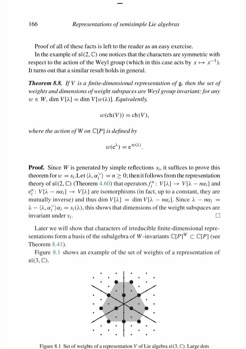
8/21/2019 Introduction to Lie Groups and Lie Algebras
http://slidepdf.com/reader/full/introduction-to-lie-groups-and-lie-algebras 178/236
166 Representations of semisimple Lie algebras
Proof of all of these facts is left to the reader as an easy exercise.
In the example of sl(2,C) one notices that the characters are symmetric with
respect to the action of the Weyl group (which in this case acts by x → x −1).
It turns out that a similar result holds in general.
Theorem 8.8. If V is a finite-dimensional representation of g , then the set of
weights and dimensions of weight subspaces are Weyl group invariant: for any
w ∈ W , dim V [λ] = dim V [w(λ)]. Equivalently,
w(ch(V ))
= ch(V ),
where the action of W on C[P] is defined by
w(eλ) = ew(λ).
Proof. Since W is generated by simple reflections si, it suffices to prove this
theorem forw
= si.Let
λ, α∨
i
= n
≥ 0; then it follows from the representation
theory of sl(2,C) (Theorem 4.60) that operators f ni : V [λ] → V [λ − nαi] anden
i : V [λ − nαi] → V [λ] are isomorphisms (in fact, up to a constant, they are
mutually inverse) and thus dim V [λ] = dim V [λ − nαi]. Since λ − nαi =λ − λ, α∨
i αi = si(λ), this shows that dimensions of the weight subspaces are
invariant under si.
Later we will show that characters of irreducible finite-dimensional repre-
sentations form a basis of the subalgebra of W -invariants C[P]W ⊂ C[P] (see
Theorem 8.41).Figure 8.1 shows an example of the set of weights of a representation of
sl(3,C).
8/21/2019 Introduction to Lie Groups and Lie Algebras
http://slidepdf.com/reader/full/introduction-to-lie-groups-and-lie-algebras 179/236
8.2. Highest weight representations and Verma modules 167
8.2. Highest weight representations and Verma modules
To study irreducible representations, we introduce a class of representations thatare generated by a single vector. As we will later show, all finite-dimensional
irreducible representations fall into this class. However, it turns out that to study
finite-dimensional representations, we need to consider infinite-dimensional
representations as an auxiliary tool.
Recall (see Theorem 7.52) that choice of polarization of the root system gives
the following decomposition for the Lie algebra g:
g = n− ⊕ h ⊕ n+, n± = α∈ R±
gα .
Definition 8.9. A non-zero representation V (not necessarily finite-
dimensional) of g is called a highest weight representation if it is generated
by a vector v ∈ V [λ] such that x .v = 0 for all x ∈ n+. In this case, v is called
the highest weight vector , and λ is the highest weight of V .
The importance of such representations is explained by the followingtheorem.
Theorem 8.10. Every irreducible finite-dimensional representation of g is a
highest weight representation.
Proof. Let P(V ) be the set of weights of V . Let λ ∈ P(V ) be such that for all
α ∈ R+, λ + α /∈ P(V ). Such a λ exists: for example, we can take h ∈ h such
that
h, α
> 0 for all α
∈ R
+, and then consider λ
∈ P(V ) such that
h, λ
is
maximal possible.
Now let v ∈ V [λ] be a non-zero vector. Since λ + α /∈ P(V ), we have
eαv = 0 for any α ∈ R+. Consider the subrepresentation V ⊂ V generated by
v. By definition, V is a highest weight representation. On the other hand, since
V is irreducible, one has V = V .
Note that there can be many non-isomorphic highest weight representations
with the same highest weight. However, in any highest weight representation
with highest weight vector vλ ∈ V [λ], the following conditions hold:

8/21/2019 Introduction to Lie Groups and Lie Algebras
http://slidepdf.com/reader/full/introduction-to-lie-groups-and-lie-algebras 180/236
168 Representations of semisimple Lie algebras
More formally, define
M λ
= U g/ I λ, (8.7)
where I λ is the left ideal in U g generated by vectors e ∈ n+ and
(h − h, λ), h ∈ h. This module is called the Verma module and plays an
important role in representation theory.
Alternatively, Verma modules can be defined as follows. Define the Borel
subalgebra b by
b = h ⊕ n+. (8.8)
Formulas (8.6) define a one-dimensional representation of b which we will
denote by Cλ. Then Verma module M λ can be defined by
M λ = U g ⊗U b Cλ. (8.9)
Remark 8.11. Readers familiar with the notion of induced representation will
recognize that M λ can be naturally described as an induced representation:
M λ = IndU gU bCλ.
Example 8.12. Let g = sl(2,C) and identify h∗ C by λ → h, λ, so thatα → 2. Then Verma module M λ, λ ∈ C, is the module described in Lemma 4.58.
The following lemma shows that Verma modules are indeed universal in a
suitable sense.
Lemma 8.13. If V is a highest weight representation with highest weight λ ,
then
V M λ/W ,
for some submodule W ⊂ M λ.
Thus, the study of highest weight representations essentially reduces to the
study of submodules in Verma modules.
Theorem 8.14. Let λ ∈ h∗ and let M λ be the Verma module with highest
weight λ.
(1) Every vector v ∈ M λ can be uniquely written in the formv = uvλ , u ∈ U n−.
I th d th
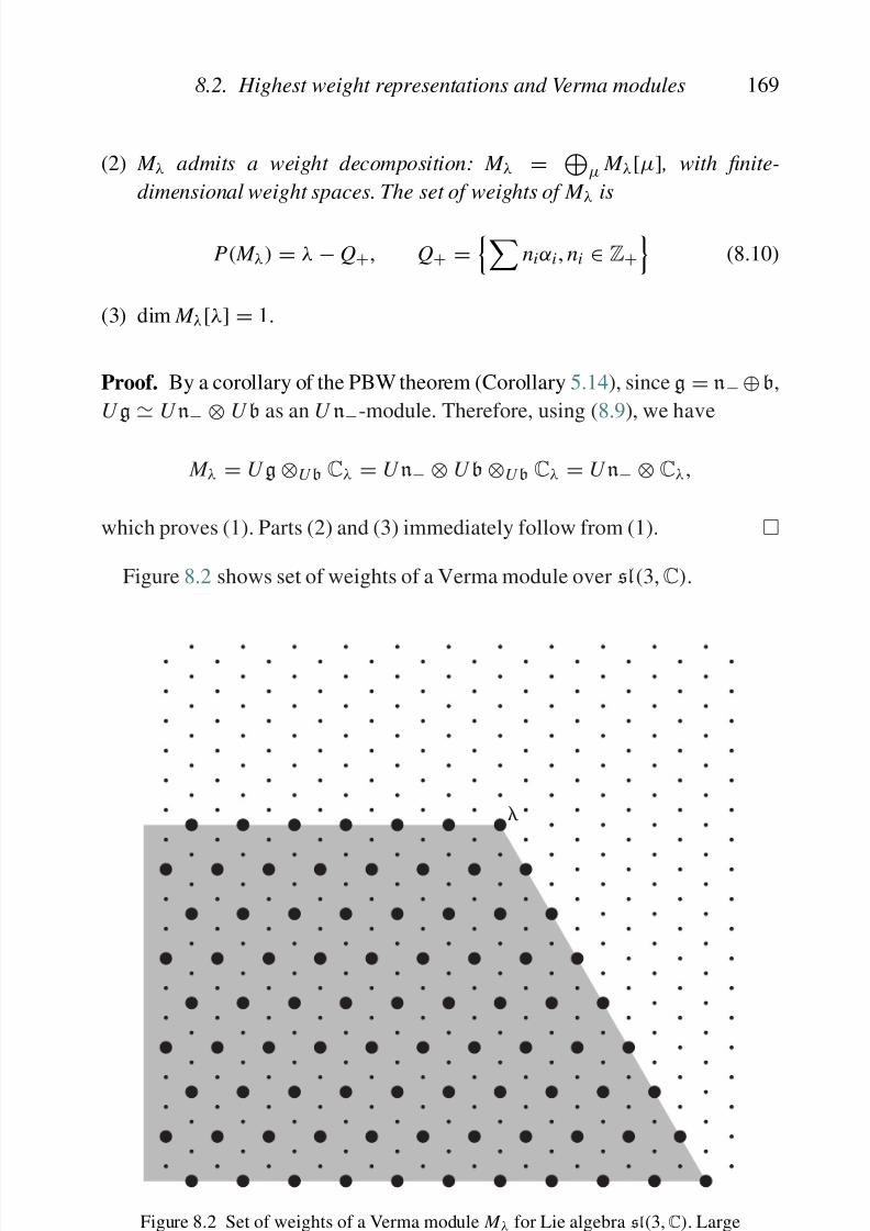
8/21/2019 Introduction to Lie Groups and Lie Algebras
http://slidepdf.com/reader/full/introduction-to-lie-groups-and-lie-algebras 181/236
8.2. Highest weight representations and Verma modules 169
(2) M λ admits a weight decomposition: M λ =
µ M λ[µ] , with finite-
dimensional weight spaces. The set of weights of M λ is
P( M λ) = λ − Q+, Q+ =
niαi, ni ∈ Z+
(8.10)
(3) dim M λ[λ] = 1.
Proof. By a corollary of the PBW theorem (Corollary 5.14), since g = n− ⊕b,
U g
U n
− ⊗U b as an U n
−-module. Therefore, using (8.9), we have
M λ = U g ⊗U b Cλ = U n− ⊗ U b ⊗U b Cλ = U n− ⊗ Cλ,
which proves (1). Parts (2) and (3) immediately follow from (1).
Figure 8.2 shows set of weights of a Verma module over sl(3,C).
8/21/2019 Introduction to Lie Groups and Lie Algebras
http://slidepdf.com/reader/full/introduction-to-lie-groups-and-lie-algebras 182/236
170 Representations of semisimple Lie algebras
Since every highest weight representation is a quotient of a Verma module, the
above theorem can be generalized to an arbitrary highest weight representation.
For future convenience, introduce relations ≺, on h∗ by
λ µ iff µ − λ ∈ Q+,
λ ≺ µ ⇐⇒ λ µ, λ = µ,(8.11)
where Q+ is defined by (8.10). It is easy to see that is a partial order on h∗.
Theorem 8.15. Let V be a highest weight representation with highest weight
λ (not necessarily finite-dimensional).
(1) Every vector v ∈ M λ can be written in the form v = uvλ , u ∈ U n−. In
other words, the map
U n− → M λ
u → uvλ
is surjective.
(2) V admits a weight decomposition: V = µλ V [µ] , with finite-
dimensional weight subspaces.
(3) dim M λ[λ] = 1.
Proof. Part (1) immediately follows from the similar statement for Verma mod-
ules. Part (2) also follows from weight decomposition for Verma modules and
the following linear algebra lemma, the proof of which is left as an exercise
(see Exercise 8.1).
Lemma 8.16. Let h be a commutative finite-dimensional Lie algebra and M
a module over h (not necessarily finite-dimensional) which admits a weight
decomposition with finite-dimensional weight spaces:
M =
M [λ], M [λ] = {v | hv = h, λv}.
Then any submodule, quotient of M also admits a weight decomposition.
8/21/2019 Introduction to Lie Groups and Lie Algebras
http://slidepdf.com/reader/full/introduction-to-lie-groups-and-lie-algebras 183/236
8.3. Classification of irreducible finite-dimensional representations 171
Proof. Indeed, if λ, µ are highest weights, then by Theorem 8.15, λ µ and
µ
λ, which is impossible unless λ
= µ.
8.3. Classification of irreducible finite-dimensional
representations
Our next goal is to classify all irreducible finite-dimensional representations.
Since by Theorem 8.10 every such representation is a highest weight represen-
tation, this question can be reformulated as follows: classify all highest weightrepresentations which are finite-dimensional and irreducible.
The first step is the following easy result.
Theorem 8.18. For any λ ∈ h∗ , there exists a unique up to isomorphism irre-
ducible highest weight representation with highest weight λ. This representation
is denoted Lλ.
Proof. All highest weight representations with highest weight λ are of theform M λ/W for some W ⊂ M λ. It is easy to see that M λ/W is irreducible iff
W is a maximal proper subrepresentation (that is, not properly contained in any
other proper subrepresentation). Thus, it suffices to prove that M λ has a unique
maximal proper submodule.
Note that by Lemma 8.16, every proper submodule W ⊂ M λ admits a weight
decomposition and W [λ] = 0 (otherwise, we would have W [λ] = M λ[λ],
which would force W
= M λ). Let J λ be the sum of all submodules W
⊂ M λ
such that W [λ] = 0. Then J λ ⊂ M λ is proper (because J λ[λ] = 0). Since itcontains every other proper submodule of M λ, it is the unique maximal proper
submodule of M λ. Thus, Lλ = M λ/ J λ is the unique irreducible highest-weight
module with highest weight λ.
Example 8.19. For g = sl(2,C), the results of Section 4.8 show that if λ ∈ Z+,
then Lλ = V λ is the finite-dimensional irreducible module of dimension λ + 1,
and Lλ
= M λ for λ /
∈Z
+.
As we will later see, the situation is similar for other Lie algebras. In particular,
8/21/2019 Introduction to Lie Groups and Lie Algebras
http://slidepdf.com/reader/full/introduction-to-lie-groups-and-lie-algebras 184/236
172 Representations of semisimple Lie algebras
Thus, to classify all irreducible finite-dimensional representations of g, we
need to find which of Lλ are finite-dimensional.
To give an answer to this question, we need to introduce some notation.
Recall the weight lattice P ⊂ h∗ defined by (7.12).
Definition 8.21. A weight λ ∈ h∗ is called dominant integral the following
condition holds
λ, α∨ ∈ Z+ for all α ∈ R+. (8.12)
The set of all dominant integral weights is denoted by P+.
It follows from results of Exercise 7.2 that condition (8.12) is equivalent to
λ, α∨i ∈ Z+ for all αi ∈ . (8.13)
Lemma 8.22.
(1) P+ = P ∩ C + , where C + = {λ ∈ h∗ | λ, α∨i > 0 ∀i} is the positive Weyl
chamber and C + is its closure.
(2) For any λ
∈ P, its Weyl group orbit W λ contains exactly one element
of P+.
Proof. The first part is immediate from the definitions. The second part follows
from the fact that any W -orbit in h∗R
contains exactly one element from C +(Exercise 7.8).
Theorem 8.23. Irreducible highest weight representation Lλ is finite-
dimensional iff λ ∈ P+.
Before proving this theorem, note that together with Theorem 8.10 it
immediately implies the following corollary.
Corollary 8.24. For every λ ∈ P+ , representation Lλ is an irreducible
finite-dimensional representation. These representations are pairwise non-
isomorphic, and every irreducible finite-dimensional representation is isomor-
phic to one of them.
Proof of Theorem 8.23. First, let us prove that if Lλ is finite-dimensional, thenλ ∈ P+. Indeed, let αi be a simple root and let sl(2,C)i be the subalgebra in g
d b h f ( L 6 42) C id L l(2 C) d l
8/21/2019 Introduction to Lie Groups and Lie Algebras
http://slidepdf.com/reader/full/introduction-to-lie-groups-and-lie-algebras 185/236
8.3. Classification of irreducible finite-dimensional representations 173
Now let us prove that if λ ∈ P+, then Lλ is finite-dimensional. This is a more
difficult result; we break the proof in several steps.
Step 1. Let ni = α∨i , λ ∈ Z+. Consider the vector
vsi .λ = f ni+1i vλ ∈ M λ[si.λ], (8.14)
where vλ ∈ M λ is the highest-weight vector and
si.λ = λ − (ni + 1)αi. (8.15)
(we will give a more general definition later, see (8.20)). Then we have
e jvsi .λ = 0 for all i, j. (8.16)
Indeed, for i = j we have [e j, f i] = 0 (see equation (7.29)), so e j f ni+1i vλ =
f ni+1i e jvλ = 0. For i = j, this follows from the results of Section 4.8: if v
is a vector of weight n in a representation of sl(2,C) such that ev = 0, then
ef
n
+1v
= 0.Step 2. Let M i ⊂ M λ be the subrepresentation generated by vector vsi .λ. By
(8.16), M i is a highest weight representation. In particular, by Theorem 8.15
all weights µ of M i must satisfy µ si.λ ≺ λ. Thus, λ is not a weight of M i;
therefore, each M i is a proper submodule in M λ.
Consider now the quotient
˜ Lλ = M λ/
M i. (8.17)
Since each M i is a proper subrepresentation, so is
M i (see the proof of
Theorem 8.18 ); thus, ˜ Lλ is a non-zero highest weight representation.
Step 3. The key step of the proof is the following theorem.
Theorem 8.25. Let λ ∈ P+ , and let ˜ Lλ be defined by (8.17). Then ˜ Lλ is finite-
dimensional.
The proof of this theorem is rather long. It is given in a separate section
(Section 8.9) at the end of this chapter.Now we can complete the proof of Theorem 8.23. Since Lλ is the quotient
8/21/2019 Introduction to Lie Groups and Lie Algebras
http://slidepdf.com/reader/full/introduction-to-lie-groups-and-lie-algebras 186/236
174 Representations of semisimple Lie algebras
useful, as it gives such a representation as a quotient of an infinite-
dimensional representation M λ. However, for all classical algebras there
also exist very explicit constructions of the irreducible finite-dimensional
representations, which are usually not based on realizing Lλ as quotients
of Verma modules. We will give an example of this for g = sl(n,C)
in Section 8.7
Example 8.26. Let g be a simple Lie algebra. Consider the adjoint represen-
tation of g, which in this case is irreducible. Weights of this representation are
exactly α
∈ R (with multiplicity 1) and 0 with multiplicity dim h
= r .
By general theory above, this representation must have a highest weight θ ,which can be defined by conditions θ ∈ R, θ + α /∈ R ∪ {0} for any α ∈ R+;
from this, it is easy to see that θ ∈ R+. Usually, θ is called the maximal root of
g. Another characterization can be found in Exercise 8.6.
In particular, for g = sl(n,C), the maximal root θ is given by θ = e1 − en.
8.4. Bernstein–Gelfand–Gelfand resolutionIn the previous section, we have shown that for λ ∈ P+, the irreducible highest
weight representation Lλ is finite-dimensional. Our next goal is to study the
structure of these representations – in particular, to find the dimensions of
weight subspaces.
Recall that in the proof of Theorem 8.23 we defined, for each λ ∈ P+, a
collection of submodules M i ⊂ M λ. We have shown that each of them is a
highest weight module. In fact, we can make a more precise statement.
Lemma 8.27. Let v ∈ M λ[µ] be a vector such that n+v = 0 (such a vector is
called a singular vector) , and let M ⊂ M λ be the submodule generated by v.
Then M is a Verma module with highest weight µ.
Proof. Since eαv = 0, by definition M is a highest weight representation with
highest weight µ and thus is isomorphic to a quotient of the Verma module M µ.
To show that M
= M µ, it suffices to show that the map U n−
→ M : u
→ uv
is injective.Indeed, assume that uv = 0 for some u ∈ U n−. On the other hand, by
8/21/2019 Introduction to Lie Groups and Lie Algebras
http://slidepdf.com/reader/full/introduction-to-lie-groups-and-lie-algebras 187/236
8.4. Bernstein–Gelfand–Gelfand resolution 175
Theorem 8.28. Let λ ∈ P+. As in the proof of Theorem 8.23 , let
vsi .λ = f ni+1i vλ ∈ M λ, ni = λ, α∨i
and let M i ⊂ M λ be the submodule generated by vsi .λ.
(1) Each M i is isomorphic to a Verma module:
M i M si .λ, si.λ = λ − (ni + 1)αi
(2)
Lλ = M λ r
i=1
M i.
Proof. Part (1) is an immediate corollary of (8.16) and Lemma 8.27. To prove
part (2), let ˜ Lλ
= M λ M i. As was shown in the proof of Theorem 8.23,
˜ Lλ is finite-dimensional, and all weights µ of ˜ Lλ satisfy µ λ. By completereducibility (Theorem 6.20),wecanwrite ˜ Lλ =
µλ, µ∈P+ nµ Lµ. Comparing
the dimensions of subspace of weight λ, we see that nλ = 1: ˜ Lλ = Lλ ⊕µ≺λ nµ Lµ
. This shows that the highest weight vector vλ of ˜ Lλ is in Lλ;
thus, the submodule it generates must be equal to Lλ. On the other hand, vλ
generates ˜ Lλ.
Example 8.29. For g
= sl(2,C), this theorem reduces to Lλ
= M λ/ M
−λ−
1,
λ ∈ Z+, which had already been established in the proof of Theorem 4.59.
Theorem 8.28 provides some description of the structure of finite-
dimensional irreducible representations Lλ. In particular, we can try to use it to
find dimensions of the weight subspaces in Lλ: indeed, for M λ dimensions of
the weight subspaces can be easily found, since by Theorem 8.14, for β ∈ Q+,
we have dim M λ[λ − β] = dim U n−[−β]. The latter dimension can be easily
found using the PBW theorem.
However, for Lie algebras other than sl(2,C), Theorem 8.28 does not give
f ll i f ti b t th t t f L i ti l it i t h t fi d

8/21/2019 Introduction to Lie Groups and Lie Algebras
http://slidepdf.com/reader/full/introduction-to-lie-groups-and-lie-algebras 188/236
176 Representations of semisimple Lie algebras
but does not describe its kernel. Since Lλ = M λ/
M i, we can extend (8.18)
to the following exact sequence of modules: M si .λ → M λ → Lλ → 0 (8.19)
which, unfortunately, is not a short exact sequence: the first map is not injective.
It turns out, however, that (8.19) can be extended to a long exact sequence,
which gives a resolution of Lλ. All terms in this resolution will be direct sums
of Verma modules.
Define the shifted action of the Weyl group W on h∗ by
w.λ = w(λ + ρ) − ρ, (8.20)
where ρ = 12
α∈ R+ α as in Lemma 7.36. Note that in particular, siρ = ρ − αi
(see proof of Lemma 7.36), so this definition agrees with earlier definition
(8.15).
Theorem 8.30. Let λ ∈ P+. Then there exists a long exact sequence
0 → M w0.λ → · · · w∈W ,l(w)=k
M w.λ · · · →i
M si .λ → M λ → Lλ → 0
where l(w) is the length of an element w ∈ W as defined in Definition 7.34 ,
and w0 is the longest element of the Weyl group (see Lemma 7.39).
This is called the Bernstein–Gelfand–Gelfand ( BGG) resolution of Lλ.
The proof of this theorem is rather hard and will not be given here. The
interested reader can find it in the original paper [2].
Example 8.31. For g = sl(2,C), W = {1, s}, and s.λ = −λ− 2 (if we identify
h∗ with C as in Example 8.12), so the BGG resolution takes the form
0 → M −λ−2 → M λ → Lλ → 0
(compare with the proof of Theorem 4.59).
Example 8.32. For g = sl(3,C
), W = S 3, and the BGG resolution takes theform
8/21/2019 Introduction to Lie Groups and Lie Algebras
http://slidepdf.com/reader/full/introduction-to-lie-groups-and-lie-algebras 189/236
8.5. Weyl character formula 177
reader we briefly list some of the exciting possibilities it opens; none of them
will be used in the remainder of this book.
• For fixed λ ∈ P+, inclusions of the modules of the form M w.λ define a partial
order on W . This order is independent of λ (as long as λ ∈ P+) and is called
Bruhat order on W .
• BGG resolution and Bruhat order are closely related to the geometry of
the flag variety F = G/ B, where G is the simply-connected complex Lie
group with Lie algebra g and B is the Borel subgroup, i.e. the subgroup
corresponding to the Borel subalgebra b; in the simplest example of G
=GL(n,C), the flag variety F was described in Example 2.25. In particular,the flag variety admits a cell decomposition in which the cells are labeled by
elements of W and the partial order defined by “cell C 1 is in the closure of
cell C 2” coincides with the Bruhat order.
• One can also ask if it is possible to write a similar resolution in terms of
Verma modules for Lλ when λ /∈ P+. It can be shown that for generic λ,
Lλ = M λ; however, there is a number of intermediate cases between generic
λ and λ
∈ P
+. It turns out that there is indeed an analog of BGG resolution for
any λ, but it is highly non-trivial; proper description of it, given by Kazhdan
and Lusztig, requires introducing a new cohomology theory (intersection
cohomology, or equivalently, cohomology of perverse sheaves) for singular
varieties such as the closures of cells in flag variety. An introduction to this
theory, with further references, can be found in [37].
8.5. Weyl character formula
Recall that for a finite-dimensional representation V we have defined its char-
acter ch(V ) by ch(V ) = dim V [λ]eλ ∈ C[P]. In this section, we will give
an explicit formula for characters of irreducible representations Lλ.
Before doing this, we will need to define characters for certain infinite-
dimensional representations; however, they will be not in C[P] but in a certain
completion of it. There are several possible completions; the one we will use is
defined by
8/21/2019 Introduction to Lie Groups and Lie Algebras
http://slidepdf.com/reader/full/introduction-to-lie-groups-and-lie-algebras 190/236
178 Representations of semisimple Lie algebras
Definition 8.4 is in C[P]. The same holds for finite direct sums of highest weight
modules.
In particular, it is very easy to compute characters of Verma modules.
Lemma 8.33. For any λ ∈ P,
ch( M λ) = eλα∈ R+ (1 − e−α)
,
where each factor 11−e−α should be understood as a formal series
11 − e−α
= 1 + e−α + e−2α + · · ·
Proof. Since u → uvλ gives an isomorphism U n− M λ (Theorem 8.14), we
see that ch( M λ) = eλ ch(U n−) (note that U n− is not a representation of g, but
it still has weight decomposition and thus we can define its character). Thus, we
need to compute the character of U n−. On the other hand, by the PBW theorem
(Theorem 5.11), monomials
α∈ R+ f nαα form a basis in U n−. Thus,
ch(U n−) = µ∈Q+
e−µP(µ),
where P(µ) is so-called Kostant partition function defined by
P(µ) =
number of ways to write µ =
α∈ R
+
nαα
(8.22)
On the other hand, explicit computation shows thatα∈ R+
1
1 − e−α =
α∈ R+
(1 + e−α + e−2α + . . . )
=
µ∈Q+
P(µ)e−µ = ch(U n−).
Now we are ready to give the celebrated Weyl character formula, which gives
the characters of irreducible highest weight representations
8/21/2019 Introduction to Lie Groups and Lie Algebras
http://slidepdf.com/reader/full/introduction-to-lie-groups-and-lie-algebras 191/236
8.5. Weyl character formula 179
Note that since we already know that Lλ is finite-dimensional the quotient is
in fact polynomial, i.e. lies in C
[P
]rather than in the completion C
[P
].
Proof. We will use the BGG resolution. Recall from linear algebra that if we
have a long exact sequence of vector spaces 0 → V 1 → · · · → V n → 0, then(−1)i dim V i = 0. Similarly, if we have a long exact sequence of g-modules,
then applying the previous argument to each weight subspace separately we see
that
(−1)i ch(V i) = 0.
Applying this to the BGG resolution, we see that
ch( Lλ) = w∈W
(−1)l(w) ch( M w.λ).
Since characters of Verma modules are given by Lemma 8.33, we get
ch( Lλ) =w∈W
(−1)l(w) ew.λ
α∈ R+(1 − e−α )
which gives the first form of Weyl character formula. To get the second form,
notice that ew.λ = ew(λ+ρ)−ρ = e−ρ ew(λ+ρ) and(1 − e−α) =
e−α/2(eα/2 − e−α/2) = e−ρ
(eα/2 − e−α/2)
since ρ = 12
α (see Lemma 7.36).
Remark 8.35. There are many proofs of Weyl character formula; in particular,
there are several proofs which are “elementary” in that they do not rely on
existence of the BGG resolution (see, for example, [22]). However, in our
opinion, the BGG resolution, while difficult to prove, provides a better insight
into the true meaning of Weyl character formula.
Corollary 8.36 (Weyl denominator identity)./2 /2
l( ) ( )
8/21/2019 Introduction to Lie Groups and Lie Algebras
http://slidepdf.com/reader/full/introduction-to-lie-groups-and-lie-algebras 192/236
180 Representations of semisimple Lie algebras
Corollary 8.37. For λ ∈ P+ ,
ch( Lλ) = Aλ+ρ / Aρ
where
Aµ =w∈W
(−1)l(w)ew(µ).
Notice that it is immediate from the Weyl denominator identity that the Weyl
denominator is skew-symmetric:
w(δ) = (−1)l(w)δ.
Thus, Weyl character formula represents a W -symmetric polynomial ch( Lλ)
as a quotient of two skew-symmetric polynomials.
Weyl character formula can also be used to compute the dimensions of
irreducible representations. Namely, since
dim V = dim V [λ] = ch(V )(0)
(considering C[P] as functions on h/2π iQ∨ using (8.5)), in theory, dimension
of Lλ can be obtained by computing the value of ch( Lλ) at t = 0. However,
Weyl character formula gives ch( Lλ) as a quotient of two polynomials, both
vanishing at t = 0; thus, computing the value of the quotient at 0 is not quite
trivial. The easiest way to do this is by introducing so-called q-dimension.
Definition 8.38. For a finite-dimensional representation V of g, define
dimq V ∈ C[q±1] by
dimq V = tr V (q2ρ ) =
λ
(dim V [λ])q2(ρ,λ),
where (· , ·) is a W -invariant symmetric bilinear form on h∗ such that (λ, µ) ∈ Zfor any λ, µ
∈ P .
Obviously, q-dimension can be easily computed from character:
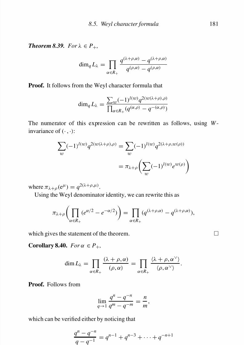
8/21/2019 Introduction to Lie Groups and Lie Algebras
http://slidepdf.com/reader/full/introduction-to-lie-groups-and-lie-algebras 193/236
8.5. Weyl character formula 181
Theorem 8.39. For λ ∈ P+ ,
dimq Lλ = α∈ R+
q(λ+ρ,α) − q(λ+ρ,α)
q(ρ,α) − q(ρ,α)
Proof. It follows from the Weyl character formula that
dimq Lλ =w
(−1)l(w)q2(w(λ+ρ),ρ)
α∈ R+ (q(α,ρ) − q−(α,ρ) )
The numerator of this expression can be rewritten as follows, using W -
invariance of (· , ·):w
(−1)l(w)q2(w(λ+ρ),ρ) =w
(−1)l(w)q2(λ+ρ,w(ρ))
= πλ+ρ
w
(−1)l(w)ew(ρ)
where πλ+ρ (eµ) = q2(λ+ρ,µ).
Using the Weyl denominator identity, we can rewrite this as
πλ+ρ
α∈ R+
(eα/2 − e−α/2)
=
α∈ R+
(q(λ+ρ,α) − q(λ+ρ,α)),
which gives the statement of the theorem.
Corollary 8.40. For α ∈ P+ ,
dim Lλ =
α∈ R+
(λ + ρ, α)
(ρ, α)=
α∈ R+
λ + ρ, α∨ρ, α∨ .
Proof. Follows from
limq→1
qn
−q−n
qm − q−m = n
m ,

8/21/2019 Introduction to Lie Groups and Lie Algebras
http://slidepdf.com/reader/full/introduction-to-lie-groups-and-lie-algebras 194/236
182 Representations of semisimple Lie algebras
It should be noted that explicitly computing characters using Weyl character
formula can lead to extremely long computations (suffices to mention that the
Weyl group of type E 8 has order 696, 729, 600). There are equivalent formu-
las which are slightly more convenient for computations, such a Freudental’s
formula (see [22]); however, with any of these formulas doing computations
by hand is extremely tedious. Fortunately, there are software packages which
allow one to delegate this job to a computer. Among the most popular are
the weyl package for Maple, developed by John Stembridge [56], the LiE
program developed by Marc van Leeuwen [35], and the GAP computational
discrete algebra system [13].
8.6. Multiplicities
Since finite-dimensional irreducible representations of g are classified by
dominant weights λ ∈ P+, it follows from complete reducibility that any
finite-dimensional representation can be written as
V = λ∈P+
nλ Lλ. (8.24)
In this section, we discuss how one can compute multiplicities nλ.
Theorem 8.41. Characters ch( Lλ) , λ ∈ P+ , form a basis in the algebra of
W -invariant polynomials C[P]W .
Proof. First, note that we have a fairly obvious basis in C[P]W . Namely, for
any λ ∈ P+ let
mλ =
µ∈W λ
eµ,
where W λ is the W -orbit of λ. Since any orbit contains a unique element of P+(Lemma 8.22), it is clear that elements mλ, λ ∈ P+, form a basis in C[P]W .
It follows from Theorem 8.15 that for any λ ∈ P+, we have
ch( Lλ) = cµeµ = mλ +
cµmµ,
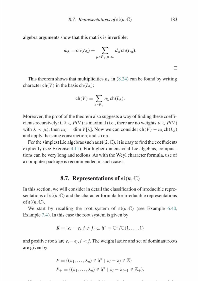
8/21/2019 Introduction to Lie Groups and Lie Algebras
http://slidepdf.com/reader/full/introduction-to-lie-groups-and-lie-algebras 195/236
8.7. Representations of sl(n,C) 183
algebra arguments show that this matrix is invertible:
mλ = ch( Lλ) + µ∈P+,µ≺λ
d µ ch( Lµ).
This theorem shows that multiplicities nλ in (8.24) can be found by writing
character ch(V ) in the basis ch( Lλ):
ch(V ) = λ∈P+
nλ ch( Lλ).
Moreover, the proof of the theorem also suggests a way of finding these coeffi-
cients recursively: if λ ∈ P(V ) is maximal (i.e., there are no weights µ ∈ P(V )
with λ ≺ µ), then nλ = dim V [λ]. Now we can consider ch(V ) − nλ ch( Lλ)
and apply the same construction, and so on.
For the simplest Lie algebras such as sl(2,C), it is easy to find the coefficients
explicitly (see Exercise 4.11). For higher-dimensional Lie algebras, computa-
tions can be very long and tedious. As with the Weyl character formula, use of
a computer package is recommended in such cases.
8.7. Representations of sl( n,C)
In this section, we will consider in detail the classification of irreducible repre-
sentations of sl(n,C) and the character formula for irreducible representationsof sl(n,C).
We start by recalling the root system of sl(n,C) (see Example 6.40,
Example 7.4). In this case the root system is given by
R = {ei − e j, i = j} ⊂ h∗ = Cn/C(1, . . . , 1)
and positive roots are ei
−e j, i < j. The weight lattice and set of dominant roots
are given by
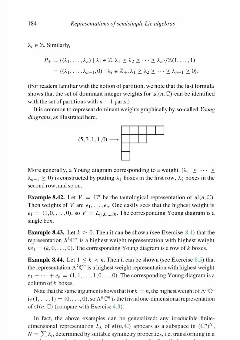
8/21/2019 Introduction to Lie Groups and Lie Algebras
http://slidepdf.com/reader/full/introduction-to-lie-groups-and-lie-algebras 196/236
184 Representations of semisimple Lie algebras
λi ∈ Z. Similarly,
P+ = {(λ1, . . . , λn) | λi ∈ Z, λ1 ≥ λ2 ≥ · · · ≥ λn}/Z(1, . . . , 1)
= {(λ1, . . . , λn−1, 0) | λi ∈ Z+, λ1 ≥ λ2 ≥ · · · ≥ λn−1 ≥ 0}.
(For readers familiar with the notion of partition, we note that the last formula
shows that the set of dominant integer weights for sl(n,C) can be identified
with the set of partitions with n − 1 parts.)
It is common to represent dominant weights graphically by so-called Young
diagrams, as illustrated here.
(5,3,1,1,0) −→
More generally, a Young diagram corresponding to a weight (λ1 ≥ · · · ≥λn−1 ≥ 0) is constructed by putting λ1 boxes in the first row, λ2 boxes in thesecond row, and so on.
Example 8.42. Let V = Cn be the tautological representation of sl(n,C).
Then weights of V are e1, . . . , en. One easily sees that the highest weight is
e1 = (1,0, . . . , 0), so V = L(1,0,...,0). The corresponding Young diagram is a
single box.
Example 8.43. Let k
≥ 0. Then it can be shown (see Exercise 8.4) that the
representation S k Cn is a highest weight representation with highest weight
ke1 = (k , 0, . . . , 0). The corresponding Young diagram is a row of k boxes.
Example 8.44. Let 1 ≤ k < n. Then it can be shown (see Exercise 8.5) that
the representation k Cn is a highest weight representation with highest weight
e1 + · · · + ek = (1, 1, . . . ,1,0, . . . 0). The corresponding Young diagram is a
column of k boxes.
Note that the same argument shows that for k
= n, the highest weight of nCn
is (1, . . . , 1) = (0, . . . , 0), so nCn is the trivial one-dimensional representationof sl(n,C) (compare with Exercise 4.3).
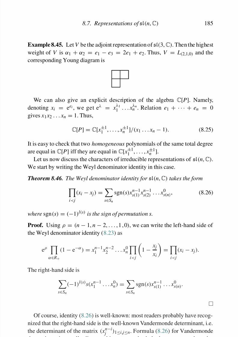
8/21/2019 Introduction to Lie Groups and Lie Algebras
http://slidepdf.com/reader/full/introduction-to-lie-groups-and-lie-algebras 197/236
8.7. Representations of sl(n,C) 185
Example 8.45. Let V be the adjoint representation of sl(3,C). Then the highest
weight of V is α1
+ α2
= e1
− e3
= 2e1
+ e2. Thus, V
= L(2,1,0) and the
corresponding Young diagram is
We can also give an explicit description of the algebra C[P]. Namely,
denoting x i = eei , we get eλ = x λ1
1 . . . x λnn . Relation e1 + · · · + en = 0
gives x 1 x 2 . . . x n = 1. Thus,
C[P] = C[ x ±11 , . . . , x ±1
n ]/( x 1 . . . x n − 1). (8.25)
It is easy to check that two homogeneous polynomials of the same total degree
are equal in C[P] iff they are equal in C[ x ±11 , . . . , x ±1
n ].
Let us now discuss the characters of irreducible representations of sl(n,C).
We start by writing the Weyl denominator identity in this case.
Theorem 8.46. The Weyl denominator identity for sl(n,C) takes the formi< j
( x i − x j) =s∈S n
sgn(s) x n−1s(1) x n−1
s(2) . . . x 0s(n), (8.26)
where sgn(s) = (−1)l(s) is the sign of permutation s.
Proof. Using ρ = (n − 1, n − 2, . . . , 1 , 0), we can write the left-hand side of
the Weyl denominator identity (8.23) as
eρ
α∈ R+
(1 − e−α) = x n−11 x n−2
2 . . . x 0n
i< j
1 − x j
x i
=i< j
( x i − x j).
The right-hand side is
s∈S n
(−1)l(s)s( x n−11 . . . x 0n) =
s∈S n
sgn(s) x n−1s(1)
. . . x 0s(n).
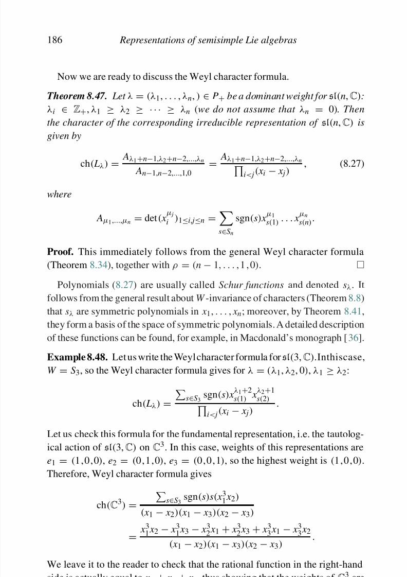
8/21/2019 Introduction to Lie Groups and Lie Algebras
http://slidepdf.com/reader/full/introduction-to-lie-groups-and-lie-algebras 198/236
186 Representations of semisimple Lie algebras
Now we are ready to discuss the Weyl character formula.
Theorem 8.47. Let λ = (λ1, . . . , λn, ) ∈ P+ be a dominant weight for sl(n,
C):λi ∈ Z+, λ1 ≥ λ2 ≥ · · · ≥ λn (we do not assume that λn = 0). Then
the character of the corresponding irreducible representation of sl(n,C) is
given by
ch( Lλ) = Aλ1+n−1,λ2+n−2,...,λn
An−1,n−2,...,1,0= Aλ1+n−1,λ2+n−2,...,λn
i< j( x i − x j), (8.27)
where
Aµ1,...,µn = det( x µ j
i )1≤i, j≤n =s∈S n
sgn(s) x µ1
s(1). . . x
µn
s(n).
Proof. This immediately follows from the general Weyl character formula
(Theorem 8.34), together with ρ = (n − 1, . . . , 1 , 0).
Polynomials (8.27) are usually called Schur functions and denoted sλ. It
follows from the general result about W -invariance of characters (Theorem 8.8)that sλ are symmetric polynomials in x 1, . . . , x n; moreover, by Theorem 8.41,
they form a basis of the space of symmetric polynomials. A detailed description
of these functions can be found, for example, in Macdonald’s monograph [36].
Example 8.48. Let us write the Weyl character formula for sl(3,C).Inthiscase,
W = S 3, so the Weyl character formula gives for λ = (λ1, λ2, 0), λ1 ≥ λ2:
ch( Lλ) = s
∈S 3
sgn(s) x λ1+2s(1)
x λ2+1s(2)
i< j( x i − x j) .
Let us check this formula for the fundamental representation, i.e. the tautolog-
ical action of sl(3,C) on C3. In this case, weights of this representations are
e1 = (1,0,0), e2 = (0,1,0), e3 = (0,0,1), so the highest weight is (1,0,0).
Therefore, Weyl character formula gives
ch(C3) = s∈
S 3
sgn(s)s( x 31 x 2)
( x 1 − x 2)( x 1 − x 3)( x 2 − x 3)
3 3 3 3 3 3
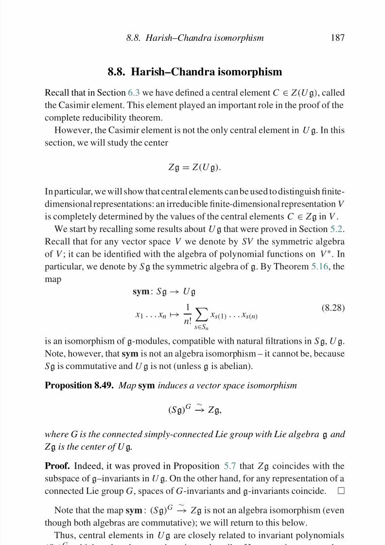
8/21/2019 Introduction to Lie Groups and Lie Algebras
http://slidepdf.com/reader/full/introduction-to-lie-groups-and-lie-algebras 199/236
8.8. Harish–Chandra isomorphism 187
8.8. Harish–Chandra isomorphism
Recall that in Section 6.3 we have defined a central element C ∈ Z (U g), calledthe Casimir element. This element played an important role in the proof of the
complete reducibility theorem.
However, the Casimir element is not the only central element in U g. In this
section, we will study the center
Z g = Z (U g).
In particular, we will show that central elements can be used to distinguish finite-dimensional representations: an irreducible finite-dimensional representation V
is completely determined by the values of the central elements C ∈ Z g in V .
We start by recalling some results about U g that were proved in Section 5.2.
Recall that for any vector space V we denote by SV the symmetric algebra
of V ; it can be identified with the algebra of polynomial functions on V ∗. In
particular, we denote by S g the symmetric algebra of g. By Theorem 5.16, the
map
sym : S g → U g
x 1 . . . x n → 1
n!s∈S n
x s(1) . . . x s(n)(8.28)
is an isomorphism of g-modules, compatible with natural filtrations in S g, U g.
Note, however, that sym is not an algebra isomorphism – it cannot be, because
S g is commutative and U g is not (unless g is abelian).
Proposition 8.49. Map sym induces a vector space isomorphism
(S g)G ∼−→ Z g,
where G is the connected simply-connected Lie group with Lie algebra g and
Z g is the center of U g.
Proof. Indeed, it was proved in Proposition 5.7 that Z g coincides with the
subspace of g–invariants in U g. On the other hand, for any representation of aconnected Lie group G, spaces of G-invariants and g-invariants coincide.
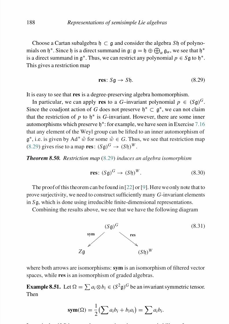
8/21/2019 Introduction to Lie Groups and Lie Algebras
http://slidepdf.com/reader/full/introduction-to-lie-groups-and-lie-algebras 200/236
188 Representations of semisimple Lie algebras
Choose a Cartan subalgebra h ⊂ g and consider the algebra S h of polyno-
mials on h∗. Since h is a direct summand in g: g
= h
⊕α gα , we see that h∗
is a direct summand in g∗. Thus, we can restrict any polynomial p ∈ S g to h∗.
This gives a restriction map
res : S g → S h. (8.29)
It is easy to see that res is a degree-preserving algebra homomorphism.
In particular, we can apply res to a G–invariant polynomial p ∈ (S g)G.
Since the coadjont action of G does not preserve h∗ ⊂
g∗, we can not claim
that the restriction of p to h∗ is G-invariant. However, there are some inner
automorphisms which preserve h∗: for example, we have seen in Exercise 7.16
that any element of the Weyl group can be lifted to an inner automorphism of
g∗, i.e. is given by Ad∗ w for some w ∈ G. Thus, we see that restriction map
(8.29) gives rise to a map res : (S g)G → (S h)W .
Theorem 8.50. Restriction map (8.29) induces an algebra isomorphism
res : (S g)G → (S h)W . (8.30)
The proof of this theorem can be found in [22] or [9]. Here we only note that to
prove surjectivity, we need to construct sufficiently many G-invariant elements
in S g, which is done using irreducible finite-dimensional representations.
Combining the results above, we see that we have the following diagram
(S g)G
sym
res
Z g (S h)W
(8.31)
where both arrows are isomorphisms: sym is an isomorphism of filtered vector
spaces, while res is an isomorphism of graded algebras.
Example 8.51. Let = ai ⊗bi ∈ (S 2g)G be an invariant symmetric tensor.
Then
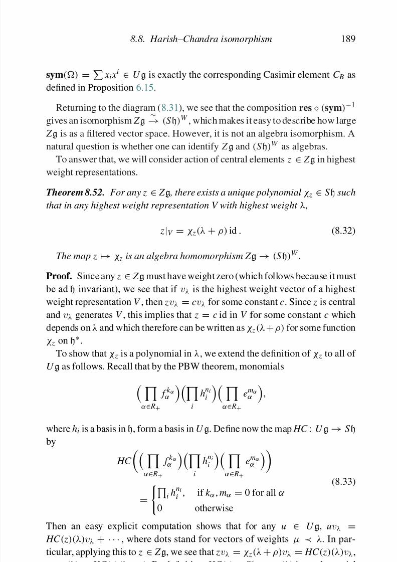
8/21/2019 Introduction to Lie Groups and Lie Algebras
http://slidepdf.com/reader/full/introduction-to-lie-groups-and-lie-algebras 201/236
8.8. Harish–Chandra isomorphism 189
sym() =
x i x i ∈ U g is exactly the corresponding Casimir element C B as
defined in Proposition 6.15.
Returning to the diagram (8.31), we see that the composition res ◦ (sym)−1
gives an isomorphism Z g ∼−→ (S h)W , which makes it easy to describe how large
Z g is as a filtered vector space. However, it is not an algebra isomorphism. A
natural question is whether one can identify Z g and (S h)W as algebras.
To answer that, we will consider action of central elements z ∈ Z g in highest
weight representations.
Theorem 8.52. For any z ∈ Z g , there exists a unique polynomial χ z ∈ S h such
that in any highest weight representation V with highest weight λ ,
z|V = χ z(λ + ρ) id . (8.32)
The map z → χ z is an algebra homomorphism Z g → (S h)W .
Proof. Since any z ∈ Z g must have weight zero (which follows because it must
be ad h invariant), we see that if vλ is the highest weight vector of a highest
weight representation V , then zvλ = cvλ for some constant c. Since z is central
and vλ generates V , this implies that z = c id in V for some constant c which
depends on λ and which therefore can be written as χ z (λ+ρ) for some function
χ z on h∗.
To show that χ z is a polynomial in λ, we extend the definition of χ z to all of
U g as follows. Recall that by the PBW theorem, monomials
α∈ R+
f k αα i
hn
ii α∈ R+
emαα ,
where hi is a basis in h, form a basis in U g. Define now the map HC : U g → S h
by
HC
α∈ R+
f k αα
i
hni
i
α∈ R+
emαα
= i hnii , if k α , mα = 0 for all α
0 otherwise
(8.33)
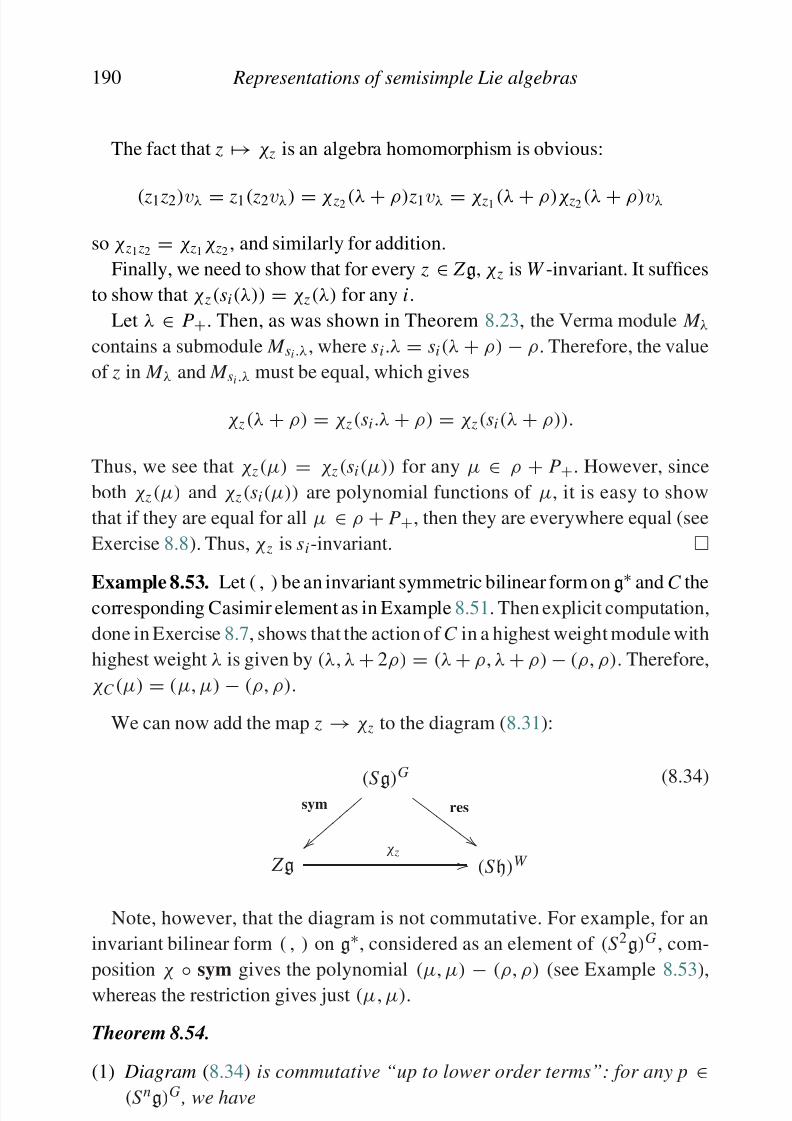
8/21/2019 Introduction to Lie Groups and Lie Algebras
http://slidepdf.com/reader/full/introduction-to-lie-groups-and-lie-algebras 202/236
190 Representations of semisimple Lie algebras
The fact that z → χ z is an algebra homomorphism is obvious:
( z1 z2)vλ = z1( z2vλ) = χ z2 (λ + ρ) z1vλ = χ z1 (λ + ρ)χ z2 (λ + ρ)vλ
so χ z1 z2 = χ z1
χ z2, and similarly for addition.
Finally, we need to show that for every z ∈ Z g, χ z is W -invariant. It suffices
to show that χ z(si(λ)) = χ z(λ) for any i.
Let λ ∈ P+. Then, as was shown in Theorem 8.23, the Verma module M λ
contains a submodule M si .λ, where si.λ = si(λ + ρ) − ρ. Therefore, the value
of z in M λ and M si .λ must be equal, which gives
χ z(λ + ρ) = χ z(si.λ + ρ) = χ z(si(λ + ρ)).
Thus, we see that χ z(µ) = χ z (si(µ)) for any µ ∈ ρ + P+. However, since
both χ z (µ) and χ z(si(µ)) are polynomial functions of µ, it is easy to show
that if they are equal for all µ ∈ ρ + P+, then they are everywhere equal (see
Exercise 8.8). Thus, χ z is si-invariant.
Example 8.53. Let ( , ) be an invariant symmetric bilinear form ong∗ and C thecorresponding Casimir element as in Example 8.51. Then explicit computation,
done in Exercise 8.7, shows that the action of C in a highest weight module with
highest weight λ is given by (λ, λ + 2ρ) = (λ + ρ, λ + ρ) − (ρ, ρ). Therefore,
χC (µ) = (µ, µ) − (ρ, ρ).
We can now add the map z → χ z to the diagram (8.31):
(S g)G
sym
res
Z gχ z
(S h)W
(8.34)
Note, however, that the diagram is not commutative. For example, for an
invariant bilinear form ( , ) on g∗, considered as an element of (S 2g)G, com-
position χ ◦
sym gives the polynomial (µ, µ) −
(ρ, ρ) (see Example 8.53),
whereas the restriction gives just (µ, µ).
8/21/2019 Introduction to Lie Groups and Lie Algebras
http://slidepdf.com/reader/full/introduction-to-lie-groups-and-lie-algebras 203/236
8.8. Harish–Chandra isomorphism 191
(2) The map χ z : Z g → (S h)W defined in Theorem 8.52 is an alge-
bra isomorphism. This isomorphism is usually called Harish–Chandra
isomorphism.
Proof. We start with part (1). It is easier to prove a more general result: for any
p ∈ S ng, we have
HC (sym( p)) ≡ res( p) mod S n−1h,
where HC : U g
→ S h is defined by (8.33).
Indeed, since sym( x 1 . . . x n) ≡ x 1 . . . x n mod U n−1g, we see that if
p =
α∈ R+
f k αα
i
hni
i
α∈ R+
emαα
∈ S ng
then we have
HC (sym( p)) ≡ i
hni
i
, k α , mα
= 0 for all α
0 otherwise = res( p) mod S n−1h.
Since for z ∈ Z g ∩ U ng we have χ z(λ) = HC ( z)(λ − ρ) ≡ HC ( z)(λ)
mod S n−1h (see proof of Theorem 8.52), we see that χ z ≡ HC ( z) mod S n−1h,
which proves part (1).
To prove part (2), note that since res is an isomorphism, part (1) implies that
composition χ ◦ sym is also an isomorphism. Since sym is an isomorphism, χ
is also an isomorphism.
Corollary 8.55. Let λ, µ ∈ h∗. Then χ z(λ) = χ z(µ) for all z ∈ Z g iff λ, µ are
in the same W -orbit.
Indeed it follows from the previous theorem and the fact that W -invariant
polynomials separate orbits of W .
Theorem 8.54 also allows one to construct an algebra isomorphism (S g)G ∼−→ Z g as a composition χ−
1
◦res. In fact, it is a special case of a more general result:for any finite-dimensional Lie algebra g there exists an algebra isomorphism
(S )G ∼Z ll d D fl Ki ill ( l D fl Gi b
8/21/2019 Introduction to Lie Groups and Lie Algebras
http://slidepdf.com/reader/full/introduction-to-lie-groups-and-lie-algebras 204/236
192 Representations of semisimple Lie algebras
to the rank of g:
(S h)W C[C 1, . . . , C r ], r = rank (g).
Degrees of the generators are also known. For various reasons it is common to
consider not degrees themselves but so-called exponents of g (or of W )
d i = deg C i − 1.
For example, for g =
sl(n,C) we have (S h)W
= (C
[ x
1, . . . , x
n]/( x
1 + · · · + x n))S n = C[σ 2, . . . , σ n], where σ i are elementary symmetric functions, i.e.
coefficients of the polynomial
( x − x i). Thus, in this case the exponents are
1, . . . , n − 1. Lists of exponents for other simple Lie algebras can be found in
[3]. We only mention here that existence of Killing form implies that d 1 = 1
for any simple Lie algebra.
Exponents also appear in many other problems related to semisimple Lie
algebras. For example, it is known that if G is a compact real semisimple Lie
group, then (topological) cohomology of G is a free exterior algebra:
H ∗(G,R) [ω1, . . . , ωr ], deg ωi = 2d i + 1,
where d i are the exponents of gC. For example, generator ω1 ∈ H 3(G) which
corresponds to d 1 = 1 is defined (up to a scalar) by Exercise 4.7. Detailed
discussion of this and related topics can be found in [14].
8.9. Proof of Theorem 8.25
In this section, we give a proof of Theorem 8.25. Recall the statement of the
theorem.
Theorem. Let λ
∈ P
+ , and let
Lλ = Mλ/
Mi
8/21/2019 Introduction to Lie Groups and Lie Algebras
http://slidepdf.com/reader/full/introduction-to-lie-groups-and-lie-algebras 205/236
8.9. Proof of Theorem 8.25 193
Definition 8.56. A representation of g is called integrable if for any v ∈ V and
any i ∈ {1, . . . , r },the sl(2,C)i-submodule generated byv is finite-dimensional:
dim(U sl(2,C)iv) < ∞.
The theorem itself follows from the following two lemmas.
Lemma 8.57. For any representation V , let
V int = {v ∈ V | For any i, dim(U sl(2,C)iv) < ∞} ⊂ V .
Then V int
is an integrable subrepresentation of V .
Lemma 8.58. Any highest weight integrable representation is finite-
dimensional.
From these two lemmas, the theorem easily follows. Indeed, consider ˜ Lλ =
M λ/
M i. Since in ˜ Lλ, f ni +1i vλ = 0 and eivλ = 0, it is easy to see that vλ
generates a finite-dimensional U sl(2,C)i–module and thus vλ ∈ ˜ Lintλ . Since vλ
generates ˜ Lλ, it follows from Lemma 8.57 that ˜ Lλ is integrable. By Lemma 8.58,
this implies that ˜ Lλ is finite-dimensional.Thus, it remains to prove these two lemmas.
Proof of Lemma 8.57. Let v ∈ V int and let W be the sl(2,C)i–module
generated by v. By assumption, W is finite-dimensional. Consider now the
vector space gW , spanned by vectors x w, x ∈ g, w ∈ W . Clearly, gW is
finite-dimensional. It is also closed under the action of sl(2,C)i:
ei x w
= xeiw
+ [ x , ei]w
∈ gW
and similarly for other elements of sl(2,C)i. Thus, we see that for any x ∈ g, x v
is contained in the finite-dimensional sl(2,C)i–module gW . Repeating this for
all i, we see that x v ∈ V int. Therefore, V int is a subrepresentation; by definition,
it is integrable.
Proof of Lemma 8.58. Let V be an integrable representation. Since any vector
is contained in a finite-dimensional sl(2,C)i–submodule, the same arguments
as in the proof of Theorem 8.8 show that the set of weights of V is W -invariant.
If we additionally assume that V is a highest weight representation with highest
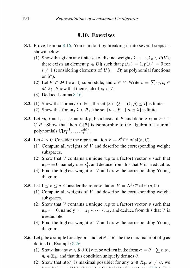
8/21/2019 Introduction to Lie Groups and Lie Algebras
http://slidepdf.com/reader/full/introduction-to-lie-groups-and-lie-algebras 206/236
194 Representations of semisimple Lie algebras
8.10. Exercises
8.1. Prove Lemma 8.16. You can do it by breaking it into several steps asshown below.
(1) Show that given any finite set of distinct weights λ1, . . . , λn ∈ P(V ),
there exists an element p ∈ U h such that p(λ1) = 1, p(λi) = 0 for
i = 1 (considering elements of U h = S h as polynomial functions
on h∗).
(2) Let V ⊂ M be an h-submodule, and v ∈ V . Write v =
vi, vi ∈
M
[λi
]. Show that then each of vi
∈ V .
(3) Deduce Lemma 8.16.
8.2. (1) Show that for any t ∈ R+, the set {λ ∈ Q+ | (λ, ρ) ≤ t } is finite.
(2) Show that for any λ ∈ P+, the set {µ ∈ P+ | µ λ} is finite.
8.3. Let ωi, i = 1, . . . , r = rank g, be a basis of P, and denote x i = eωi ∈C[P]. Show that then C[P] is isomorphic to the algebra of Laurent
polynomials C[ x ±11 , . . . , x ±1
r ].
8.4. Let k > 0. Consider the representation V = S k
Cn
of sl(n,C).(1) Compute all weights of V and describe the corresponding weight
subspaces.
(2) Show that V contains a unique (up to a factor) vector v such that
n+v = 0, namely v = x k 1 , and deduce from this that V is irreducible.
(3) Find the highest weight of V and draw the corresponding Young
diagram.
8.5. Let 1 ≤ k ≤ n. Consider the representation V =
k Cn
of sl(n,C
).(1) Compute all weights of V and describe the corresponding weight
subspaces.
(2) Show that V contains a unique (up to a factor) vector v such that
n+v = 0, namely v = x 1 ∧ · · · ∧ x k , and deduce from this that V is
irreducible.
(3) Find the highest weight of V and draw the corresponding Young
diagram.
8.6. Let g be a simple Lie algebra and let θ ∈ R+ be the maximal root of g as
defined in Example 8 26
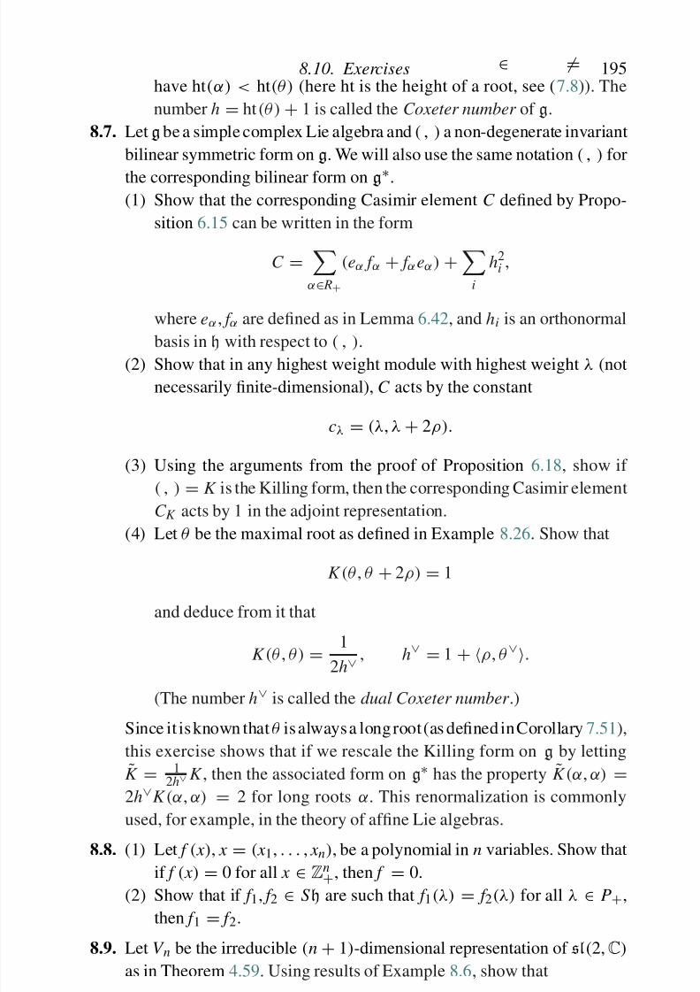
8/21/2019 Introduction to Lie Groups and Lie Algebras
http://slidepdf.com/reader/full/introduction-to-lie-groups-and-lie-algebras 207/236
8.10. Exercises 195
8.7. Let g be a simple complex Lie algebra and ( , ) a non-degenerate invariant
bilinear symmetric form on g. We will also use the same notation ( , ) for
the corresponding bilinear form on g∗.
(1) Show that the corresponding Casimir element C defined by Propo-
sition 6.15 can be written in the form
C =
α∈ R+
(eα f α + f α eα) +
i
h2i ,
where eα, f α are defined as in Lemma 6.42, and hi is an orthonormal
basis in h with respect to ( , ).(2) Show that in any highest weight module with highest weight λ (not
necessarily finite-dimensional), C acts by the constant
cλ = (λ, λ + 2ρ).
(3) Using the arguments from the proof of Proposition 6.18, show if
( , ) = K is the Killing form, then the corresponding Casimir element
C K
acts by 1 in the adjoint representation.
(4) Let θ be the maximal root as defined in Example 8.26. Show that
K (θ , θ + 2ρ) = 1
and deduce from it that
K (θ , θ ) = 1
2h∨ , h∨ = 1 + ρ, θ ∨.
(The number h∨ is called the dual Coxeter number .)
Since it is known that θ is always a long root (as defined in Corollary 7.51),
this exercise shows that if we rescale the Killing form on g by letting
K = 12h∨ K , then the associated form on g∗ has the property K (α, α) =
2h∨K (α, α) = 2 for long roots α. This renormalization is commonly
used, for example, in the theory of affine Lie algebras.
8.8. (1) Let f ( x ), x
= ( x 1, . . . , x n), be a polynomial in n variables. Show that
if f ( x ) = 0 for all x ∈ Zn+, then f = 0.
(2) Show that if f1, f2 ∈ Sh are such that f1(λ) = f2(λ) for all λ ∈ P+,

8/21/2019 Introduction to Lie Groups and Lie Algebras
http://slidepdf.com/reader/full/introduction-to-lie-groups-and-lie-algebras 208/236
196 Representations of semisimple Lie algebras
where the direct sum is over all k ∈ Z+ satisfying the Clebsh–Gordan
condition
|n − m| ≤ k ≤ n + m
n + m − k ∈ 2Z
8.10. Define a bilinear form ( , )1 on C[P] by
( f , g)1 = 1
|W
| f gδδ ,
where involution is defined by eλ = e−λ, δ is the Weyl denominator
(8.23), and
: C[P] → C is defined by
eλ =
1, λ = 0
0 otherwise.
(1) Show that ( , )1 is symmetric.
(2) Using Weyl character formula, show that characters ch( Lλ), λ ∈ P+,
are orthonormal with respect to this form.
8/21/2019 Introduction to Lie Groups and Lie Algebras
http://slidepdf.com/reader/full/introduction-to-lie-groups-and-lie-algebras 209/236
Overview of the literature
In this chapter we put together an overview of the literature and some sugges-
tions for further reading. The list is divided into three sections: textbooks (books
suitable for readers just learning the theory), monographs (books that provide
detailed coverage but which still can be classified as “core” theory of Lie groups
and Lie algebras) and “Further reading”. Needless to say, this division is rather
arbitrary and should not be taken too seriously.
Basic textbooks
There is a large number of textbooks on Lie groups and Lie algebras. Below
we list some standard references which can be used either to complement the
current book or to replace it.
Basic theory of Lie groups (subgroups, exponential map, etc.) can be found
in any good book on differential geometry, such as Spivak [49] or Warner [55].
For more complete coverage, including discussion of representation theory,
the classic references are Bröcker and tom Dieck [4] or the book by Fulton
and Harris [11]. Other notable books in this category include Varadarajan [51],
Onishchik and Vinberg [41]. The latest (and highly recommended) additions to
this list are Bump [5], Sepanski [44] and Procesi [43]. Each of these books has
its own strengths and weaknesses; we suggest that the reader looks at them tochoose the book which best matches his tastes.
F Li l b d i i l i i l Li l b b bl h
8/21/2019 Introduction to Lie Groups and Lie Algebras
http://slidepdf.com/reader/full/introduction-to-lie-groups-and-lie-algebras 210/236
198 Overview of the literature
Monographs
For readers who have learned the basic theory covered in this book or in thetextbooks listed above and want to go deeper, there is no shortage of excellent
in-depth books. Here are some notable titles.
For the foundations of the theory of Lie groups, the reader may consult Serre
[46] and Duistermaat and Kolk [10], or the classical book by Chevalley [7].
A detailed exposition of the structure theory of Lie groups, including semisimple
Lie groups, can be found in Knapp [32] or in Zhelobenko [57]; Helgason [18], in
addition to providing an introduction to theory of Lie groups and Lie algebras,
also includes a wealth of information about structure theory of Lie groups andhomogeneous spaces.
An overview of representation theory, including the theory of infinite-
dimensional representations, can be found in Kirillov [29].
Closely related to the theory of Lie groups is the theory of algebraic groups;
good introduction can be found in Springer [50].
For Lie algebras, Jacobson [24] provides a comprehensive monograph on Lie
algebras; in particular, there the reader can find the proofs of all the results on Lie
algebras whose proof we chose to skip in our book. An equally comprehensive
exposition can be found in Bourbaki [3]. For the study of universal enveloping
algebras, the best source is Dixmier [9].
A detailed exposition of the theory of root systems, Weyl groups and closely
related Coxeter groups can be found in Humphreys [23].
Further reading
In this section, we list some more advanced topics which might be of interest
to readers who have mastered basic theory of Lie groups and Lie algebras. This
list is highly biased and reflects the author’s preferences; doubtless other people
would suggest other topics.
Infinite-dimensional Lie groups and algebras
So far we have only discussed finite-dimensional Lie groups and Lie algebras.
I l h d f i fi i di i l Li d Li l b i

8/21/2019 Introduction to Lie Groups and Lie Algebras
http://slidepdf.com/reader/full/introduction-to-lie-groups-and-lie-algebras 211/236
Further reading 199
topics can be found in Kac’s book [26] and those of Pressley and Segal [42]
and Kumar [33].
Quantum groups
One of the most interesting developments in the theory of Lie groups and Lie
algebras in recent years is related to objects which are not actually Lie algebras
or groups but rather certain deformations of them. These deformations, called
“quantum groups”, are associative algebras where multiplication depends on
an extra parameter q and which for q = 1 coincide with the usual universalenveloping algebra U g. It turns out that these quantum groups have a very inter-
esting representation theory, with many features that do not appear for the usual
Lie algebras. They also appear in many applications: to physics (where they
again appear as groups of symmetries in conformal field theory), to topology
(they can be used to construct invariants of knots and three-manifolds, such
as the famous Jones polynomial), to combinatorics (special polynomials), and
much more. A good introduction to quantum groups can be found in the books
of Jantzen [25] or Kassel [28].
Analysis on homogeneous spaces
We have briefly discussed the analysis on compact Lie groups in Section 4.7.
In particular, we mentioned that the Peter–Weyl theorem should be regarded as
a non-commutative analog of the Fourier series.
However, this is just the beginning. One can also study various classes of functions on non-compact Lie groups, or on various homogeneous spaces
for G, study invariant differential operators on such spaces, integral trans-
forms, and much more. This is commonly referred to as “harmonic analysis
on homogeneous spaces”. The classical reference for the geometry of homo-
geneous spaces is Helgason [18]; analysis on such spaces is discussed in
Helgason [20] and [19]. Other notable references include Molchanov [38] and
Warner [54].
8/21/2019 Introduction to Lie Groups and Lie Algebras
http://slidepdf.com/reader/full/introduction-to-lie-groups-and-lie-algebras 212/236
200 Overview of the literature
more manageable but by no means trivial. A large program of study of infinite-
dimensional unitary representations of real reductive groups has been initiated
by Vogan; an overview of results can be found in [53].
Special functions and combinatorics
Representation theory of Lie groups and Lie algebras is intimately related
with combinatorics. For many groups, matrix coefficients and the characters
of certain representations can be explicitly written in terms of classical special
functions and orthogonal polynomials; thus, various results from representation
theory (such as orthogonality relation for matrix coefficients) become identities
involving such functions.
Representation theory of sl(n,C) is especially closely related to combina-
torics: as was mentioned in Section 8.7, irreducible representations of sl(n,C)
are parametrized by Young diagrams, which are one of the central objects of
study in combinatorics, and characters of irreducible representations are Schur
polynomials.
A detailed study of various links between the theory of special func-tions, combinatorics, and representation theory can be found in Klimyk and
Vilenkin [31].
Geometric representation theory
An extremely fruitful approach to representation theory comes from geometry:
instead of describing representations algebraically, by generators and relations,
they are constructed in geometric terms – for example, as spaces of global
sections of certain vector bundles on a manifold with the action of the group.
This approach leads to some truly remarkable results. The simplest example
of such a construction is the Borel–Weil theorem, which states that any irre-
ducible finite-dimensional representation of a semisimple complex group can
be obtained as a space of global sections of a certain line bundle Lλ over the cor-
responding flag variety; in fact, line bundles over the flag variety are classified
by integral weights (see [44]).This result has a far-reaching generalization: one can construct all highest
i h d l ( ibl i fi i di i l) if l li b dl b
8/21/2019 Introduction to Lie Groups and Lie Algebras
http://slidepdf.com/reader/full/introduction-to-lie-groups-and-lie-algebras 213/236
Further reading 201
of so called “Schubert cells” in the flag variety (since these cells are not mani-
folds but have singularities, appropriate cohomology theory is not the usual de
Rham or singular cohomology, but more complicated one, called intersection
cohomology). An introduction to this theory can be found in Milicic [37].
Another good reference for geometric methods in representation theory
is Chriss and Ginzburg [8]; however, this book is more concerned with
representations of Hecke algebras than Lie groups.
8/21/2019 Introduction to Lie Groups and Lie Algebras
http://slidepdf.com/reader/full/introduction-to-lie-groups-and-lie-algebras 214/236
Appendix A
Root systems and simple Lie algebras
In this appendix, for each of the Dynkin diagrams of types An, . . . Dn, we give
an explicit description of the corresponding root system and simple Lie algebra,
along with some relevant information such as the description of the Weyl group.
This section contains no proofs; we refer the reader to [3], [24] for proofs and
descriptions of exceptional root systems E 6, . . . , G2.In this appendix, we use the following notation.
g: a complex simple Lie algebra, with fixed Cartan subalgebra h ⊂ g.
R ⊂ h∗: the root system of g.
E = h∗R
: the real vector space spanned by roots.
( , ): the symmetric invariant bilinear form onh∗ normalized so that (α, α) =2 for long roots.
R+: set of positive roots (of course, there are many ways to choose it; we
will only give the most common and widely used choice). = {α1, . . . , αr }, r = rank ( R): set of simple roots (see Definition 7.12).
W : the Weyl group (see Section 7.2).
P ⊂ E : the weight lattice (see Section 7.5).
Q ⊂ E : the root lattice (see Section 7.5).
θ : the highest root (see Example 8.26).
ρ = 12
R+ α (see (7.22)).
h
= ht(θ )
+1, h∨
= ρ, θ ∨
+1: Coxeter number and dual Coxeter number,
see Exercise 8.6, Exercise 8.7.
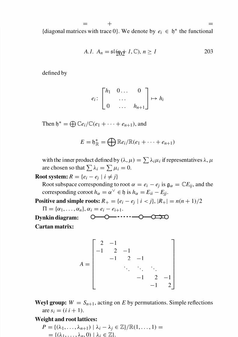
8/21/2019 Introduction to Lie Groups and Lie Algebras
http://slidepdf.com/reader/full/introduction-to-lie-groups-and-lie-algebras 215/236
A.1. An = sl(n + 1,C) , n ≥ 1 203
defined by
ei :
h1 0 . . . 0
. . .
0 . . . hn+1
→ hi
Then h∗ =Cei/C(e1 + · · · + en+1), and
E
= h∗R
=Rei/R(e1
+ · · · +en
+1)
with the inner product defined by (λ, µ) =λiµi if representatives λ, µ
are chosen so that
λi =
µi = 0.
Root system: R = {ei − e j | i = j}Root subspace corresponding to root α = ei − e j is gα = C E ij, and the
corresponding coroot hα = α∨ ∈ h is hα = E ii − E jj.
Positive and simple roots: R+ = {
ei
−e j
| i < j
},
| R
+| = n(n
+1)/2
= {α1, . . . , αn}, αi = ei − ei+1.
Dynkin diagram:
Cartan matrix:
A =
2 −1
−1 2 −1
−1 2
−1
. . . . . . . . .
−1 2 −1
−1 2
Weyl group: W = S n+1, acting on E by permutations. Simple reflections
are si = (i i + 1).
Weight and root lattices:
P = {(λ1, . . . , λn+1) | λi − λ j ∈ Z}/R(1, . . . , 1) ={(λ λ 0) | λ ∈ Z}
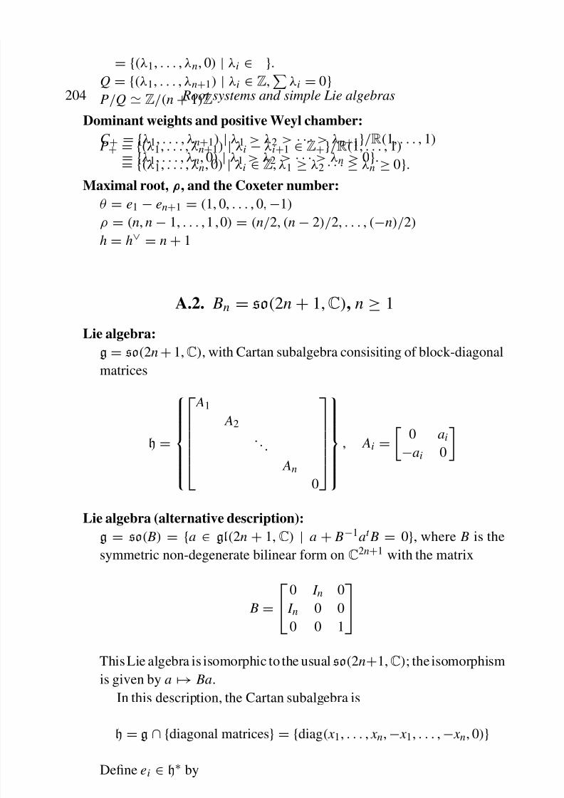
8/21/2019 Introduction to Lie Groups and Lie Algebras
http://slidepdf.com/reader/full/introduction-to-lie-groups-and-lie-algebras 216/236
204 Root systems and simple Lie algebras
P+ = {(λ1, . . . , λn+1) | λi − λi+1 ∈ Z+}/R(1, . . . , 1)
= {(λ1, . . . , λn, 0)
| λi
∈Z, λ1
≥ λ2
· · · ≥ λn
≥ 0
}.
Maximal root, ρ, and the Coxeter number:
θ = e1 − en+1 = (1, 0, . . . , 0, −1)
ρ = (n, n − 1, . . . , 1 , 0) = (n/2, (n − 2)/2, . . . , (−n)/2)
h = h∨ = n + 1
A.2. Bn
= so(2n
+1,C), n
≥ 1
Lie algebra:
g = so(2n + 1,C), with Cartan subalgebra consisiting of block-diagonal
matrices
h
=
A1
A2
. . .
An
0
, Ai
= 0 ai
−ai 0Lie algebra (alternative description):
g = so( B) = {a ∈ gl(2n + 1,C) | a + B−1at B = 0}, where B is the
symmetric non-degenerate bilinear form on C2n+1 with the matrix
B = 0 I n 0
I n 0 0
0 0 1
This Lie algebra is isomorphic to the usual so(2n+1,C); the isomorphism
is given by a → Ba.
In this description, the Cartan subalgebra is
h = g ∩ {diagonal matrices} = {diag( x 1, . . . , x n, − x 1, . . . , − x n, 0)}∗
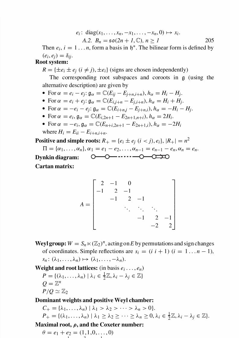
8/21/2019 Introduction to Lie Groups and Lie Algebras
http://slidepdf.com/reader/full/introduction-to-lie-groups-and-lie-algebras 217/236
A.2. Bn = so(2n + 1,C) , n ≥ 1 205
Root system:
R
= {±ei
±e j (i
= j),
±ei
}(signs are chosen independently)
The corresponding root subspaces and coroots in g (using the
alternative description) are given by
• For α = ei − e j: gα = C( E ij − E j+n,i+n), hα = H i − H j.
• For α = ei + e j: gα = C( E i, j+n − E j,i+n), hα = H i + H j.
• For α = −ei − e j: gα = C( E i+n, j − E j+n,i), hα = − H i − H j.
• For α = ei, gα = C( E i,2n+1 − E 2n+1,n+i), hα = 2 H i.
• For α = −ei, gα = C( E n+i,2n+1 − E 2n+1,i), hα = −2 H i
where H i =
E ii −
E i+n,i+n
.
Positive and simple roots: R+ = {ei ± e j (i < j), ei}, | R+| = n2
= {α1, . . . , αn}, α1 = e1 − e2, . . . , αn−1 = en−1 − en, αn = en.
Dynkin diagram:
Cartan matrix:
A =
2 −1 0
−1 2
−1
−1 2 −1
. . . . . .
. . .
−1 2 −1
−2 2
Weyl group: W = S n(Z2)n, acting on E by permutations and sign changes
of coordinates. Simple reflections are si = (i i + 1) (i = 1 . . . n − 1),sn : (λ1, . . . , λn) → (λ1, . . . , −λn).
Weight and root lattices: (in basis ei . . . , en)
P = {(λ1, . . . , λn) | λi ∈ 12Z, λi − λ j ∈ Z}
Q = Zn
P/Q Z2
Dominant weights and positive Weyl chamber:
C
+ = {λ1, . . . , λn)
| λ1 > λ2 >
· · · > λn > 0
}.
P+ = {(λ1, . . . , λn) | λ1 ≥ λ2 ≥ · · · ≥ λn ≥ 0, λi ∈ 12Z, λi − λ j ∈ Z}.
Maximal root ρ and the Coxeter number:
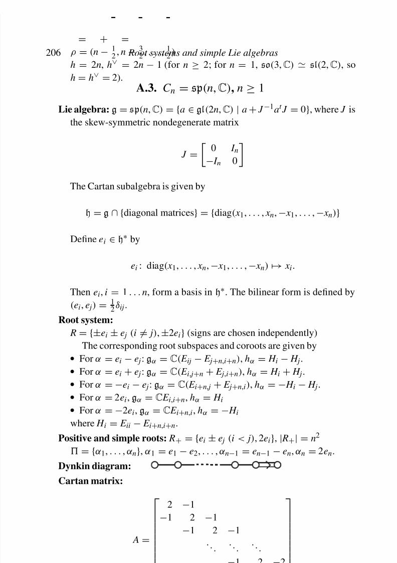
8/21/2019 Introduction to Lie Groups and Lie Algebras
http://slidepdf.com/reader/full/introduction-to-lie-groups-and-lie-algebras 218/236
206 Root systems and simple Lie algebras
A.3. C n = sp(n,C), n ≥ 1
Lie algebra: g = sp(n,C) = {a ∈ gl(2n,C) | a + J −1
at
J = 0}, where J isthe skew-symmetric nondegenerate matrix
J =
0 I n
− I n 0
The Cartan subalgebra is given by
h = g ∩ {diagonal matrices} = {diag( x 1, . . . , x n, − x 1, . . . , − x n)}
Define ei ∈ h∗ by
ei : diag( x 1, . . . , x n, − x 1, . . . , − x n) → x i.
Then ei, i = 1 . . . n, form a basis in h∗. The bilinear form is defined by
(ei, e j) = 1
2 δij .Root system:
R = {±ei ± e j (i = j), ±2ei} (signs are chosen independently)
The corresponding root subspaces and coroots are given by
• For α = ei − e j: gα = C( E ij − E j+n,i+n), hα = H i − H j.
• For α = ei + e j: gα = C( E i, j+n + E j,i+n), hα = H i + H j.
• For α = −ei − e j: gα = C( E i+n, j + E j+n,i), hα = − H i − H j.
• For α
= 2ei, gα
=C E i,i
+n, hα
= H i
• For α = −2ei, gα = C E i+n,i, hα = − H i
where H i = E ii − E i+n,i+n.
Positive and simple roots: R+ = {ei ± e j (i < j), 2ei}, | R+| = n2
= {α1, . . . , αn}, α1 = e1 − e2, . . . , αn−1 = en−1 − en, αn = 2en.
Dynkin diagram:
Cartan matrix:
2 −1−1 2 −1
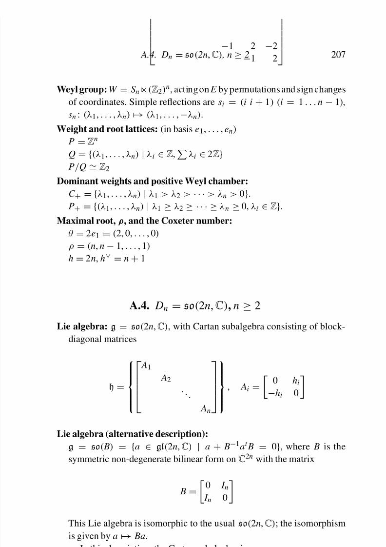
8/21/2019 Introduction to Lie Groups and Lie Algebras
http://slidepdf.com/reader/full/introduction-to-lie-groups-and-lie-algebras 219/236
A.4. Dn = so(2n,C) , n ≥ 2 207
Weyl group: W = S n(Z2)n, acting on E by permutations and sign changes
of coordinates. Simple reflections are si
= (i i
+ 1) (i
= 1 . . . n
− 1),
sn : (λ1, . . . , λn) → (λ1, . . . , −λn).
Weight and root lattices: (in basis e1, . . . , en)
P = Zn
Q = {(λ1, . . . , λn) | λi ∈ Z,
λi ∈ 2Z}P/Q Z2
Dominant weights and positive Weyl chamber:
C + = {λ1, . . . , λn) | λ1 > λ2 > · · · > λn > 0}.
P+ = {(λ1, . . . , λn) | λ1 ≥ λ2 ≥ · · · ≥ λn ≥ 0, λi ∈ Z}.Maximal root, ρ, and the Coxeter number:
θ = 2e1 = (2, 0, . . . , 0)
ρ = (n, n − 1, . . . , 1)
h = 2n, h∨ = n + 1
A.4. Dn = so(2n,C), n ≥ 2
Lie algebra: g = so(2n,C), with Cartan subalgebra consisting of block-
diagonal matrices
h =
A1
A2
. .
. An
, Ai =
0 hi
−hi 0
Lie algebra (alternative description):
g = so( B) = {a ∈ gl(2n,C) | a + B−1at B = 0}, where B is the
symmetric non-degenerate bilinear form on C2n with the matrix
B = 0 I n
I n 0
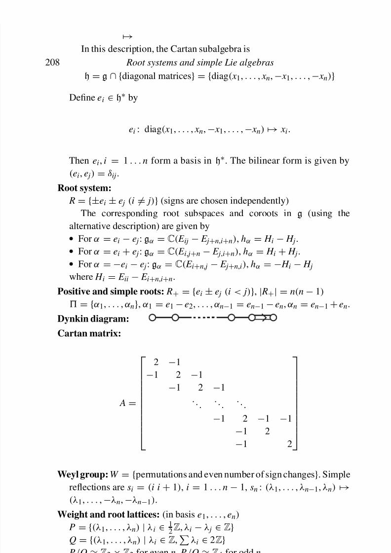
8/21/2019 Introduction to Lie Groups and Lie Algebras
http://slidepdf.com/reader/full/introduction-to-lie-groups-and-lie-algebras 220/236
208 Root systems and simple Lie algebras
Define ei ∈ h∗ by
ei : diag( x 1, . . . , x n, − x 1, . . . , − x n) → x i.
Then ei, i = 1 . . . n form a basis in h∗. The bilinear form is given by
(ei, e j) = δij.
Root system:
R = {±ei ± e j (i = j)} (signs are chosen independently)
The corresponding root subspaces and coroots in g (using thealternative description) are given by
• For α = ei − e j: gα = C( E ij − E j+n,i+n), hα = H i − H j.
• For α = ei + e j: gα = C( E i, j+n − E j,i+n), hα = H i + H j.
• For α = −ei − e j: gα = C( E i+n, j − E j+n,i), hα = − H i − H j
where H i = E ii − E i+n,i+n.
Positive and simple roots: R+ = {ei ± e j (i < j)}, | R+| = n(n − 1)
= {α1, . . . , αn
}, α1
= e1
−e2, . . . , αn
−1
= en
−1
−en, αn
= en
−1
+en.
Dynkin diagram:
Cartan matrix:
A
=
2 −1
−1 2 −1
−1 2 −1
. . . . . .
. . .
−1 2 −1 −1
−1 2
−1 2
Weyl group: W = {permutations and even number of sign changes}. Simple
reflections are si = (i i + 1), i = 1 . . . n − 1, sn : (λ1, . . . , λn−1, λn) →(λ1, . . . ,
−λn,
−λn
−1).
Weight and root lattices: (in basis e1, . . . , en)
P {(λ λ ) | λ ∈ 1Z λ λ ∈ Z}
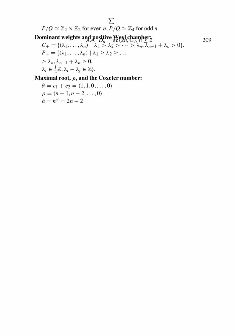
8/21/2019 Introduction to Lie Groups and Lie Algebras
http://slidepdf.com/reader/full/introduction-to-lie-groups-and-lie-algebras 221/236
A.4. Dn = so(2n,C) , n ≥ 2 209
≥ λn, λn−1 + λn ≥ 0,
λi
∈ 12Z, λi
−λ j
∈Z
}.
Maximal root, ρ, and the Coxeter number:
θ = e1 + e2 = (1,1,0, . . . , 0)
ρ = (n − 1, n − 2, . . . , 0)
h = h∨ = 2n − 2
8/21/2019 Introduction to Lie Groups and Lie Algebras
http://slidepdf.com/reader/full/introduction-to-lie-groups-and-lie-algebras 222/236
Appendix B
Sample syllabus
In this section, we give a sample syllabus of a one-semester graduate course on
Lie groups and Lie algebras based on this book. This course is designed to fit
the standard schedule of US universities: 14 week semester, with two lectures
a week, each lecture 1 hour and 20 minutes long.
Lecture 1: Introduction. Definition of a Lie group; C 1 implies analytic.
Examples: Rn, S 1, SU(2). Theorem about closed subgroup (no proof).
Connected component and universal cover.
Lecture 2: G/ H . Action of G on manifolds; homogeneous spaces. Action
on functions, vector fields, etc. Left, right, and adjoint action. Left, right,
and bi-invariant vector fields (forms, etc).
Lecture 3: Classical groups: GL, SL, SU, SO, Sp – definition. Exponentialand logarithmic maps for matrix groups. Proof that classical groups are
smooth; calculation of the corresponding Lie algebra and dimension.
Topological information (connectedness, π1). One-parameter subgroups
in a Lie group: existence and uniqueness.
Lecture 4: Lie algebra of a Lie groups:
g = T 1G = right-invariant vector fields = 1-parameter subgroups.
8/21/2019 Introduction to Lie Groups and Lie Algebras
http://slidepdf.com/reader/full/introduction-to-lie-groups-and-lie-algebras 223/236
Sample syllabus 211
[ x , y] = xy − yx for matrix algebras. Relation with the commutator of
vector fields. Campbell–Hausdorff formula (no proof).
Lecture 6: If G1 is simply-connected, then Hom(G1, G2) = Hom(g1, g2).
Analytic subgroups and Lie subalgebras. Ideals ing and normal subgroups
in G.
Lecture 7: Lie’s third theorem (no proof). Corollary: category of con-
nected, simply-connected Lie groups is equivalent to the category of Lie
algebras. Representations of G = representations of g. Action by vector
fields.Example: representations of SO(3), SU(2). Complexification; su(n)
and sl(n).
Lecture 8: Representations of Lie groups and Lie algebras. Subrepre-
sentations, direct sums, V 1 ⊗ V 2, V ∗, action on End V . Irreducibility.
Intertwining operators. Schur lemma. Semisimplicity.
Lecture 9: Unitary representations. Complete reducibility of representa-
tion for a group with invariant integral. Invariant integral for finite groupsand for compact Lie groups; Haar measure. Example: representations of
S 1 and Fourier series.
Lecture 10: Characters and Peter–Weyl theorem.
Lecture 11: Universal enveloping algebra. Central element J 2 x + J 2 y + J 2 z ∈U so(3,R). Statement of PBW theorem.
Lecture 12: Structure theory of Lie algebras: generalities. Commutant.Solvable and nilpotent Lie algebras: equivalent definitions. Example:
upper triangular matrices. Lie theorem (about representations of a
solvable Lie algebra).
Lecture 13: Engel’s theorem (without proof). Radical. Semisimple Lie
algebras. Example: semisimplicity of sl(2). Levi theorem (without
proof). Statement of Cartan criterion of solvability and semisimplicity.
Lecture 14: Jordan decomposition (into semisimple and nilpotent ele-
ment) Proof of Cartan criterion

8/21/2019 Introduction to Lie Groups and Lie Algebras
http://slidepdf.com/reader/full/introduction-to-lie-groups-and-lie-algebras 224/236
212 Sample syllabus
Lecture 16: Complete reducibility of representations of a semisimple Lie
algebra.
Lecture 17: Representations of sl(2,C). Semisimple elements in a Lie
algebra.
Lecture 18: Semisimple and nilpotent elements; Jordan decomposition.
Toral subalgebras. Definition of Cartan (maximal toral) subalgebra.
Theorem: conjugacy of Cartan subalgebras (no proof).
Lecture 19: Root decomposition and root system for semisimple Lie
algebra. Basic properties. Example: sl(n,C).
Lecture 20: Definition of an abstract root system. Weyl group. Classifica-
tion of rank 2 root systems.
Lecture 21: Positive roots and simple roots. Polarizations and Weyl
chambers. Transitivity of action of W on the set of Weyl chambers.
Lecture 22: Simple reflections. Reconstructing root system from set of
simple roots. Length l (w
) and its geometric interpretation as number of separating hyperplanes.
Lecture 23: Cartan matrix and Dynkin diagrams. Classification of Dynkin
diagrams (partial proof).
Lecture 24: Constructing a semisimple Lie algebra from a root system.
Serre relations and Serre theorem (no proof). Classification of simple Lie
algebras.
Lecture 25: Finite-dimensional representations of a semi-simple Lie
algebra. Weights; symmetry under Weyl group. Example: sl(3,C).
Singular vectors.
Lecture 26: Verma modules and irreducible highest weight modules. Dom-
inant weights and classification of finite-dimensional highest weight
modules (without proof)
Lecture 27: BGG resolution and Weyl character formula
Lecture 28: Example: representations of sl(n,C).
8/21/2019 Introduction to Lie Groups and Lie Algebras
http://slidepdf.com/reader/full/introduction-to-lie-groups-and-lie-algebras 225/236
List of notation
R: real numbers
C: complex numbers
K: either R or C. This notation is used when a result holds for both R
and C.
Z: integer numbers
Z
+ = {0,1,2, . . .
}: non-negative integer numbers
Linear algebra
V ∗: dual vector space
, : V ⊗ V ∗ → C: canonical pairing of V with V ∗.
Hom(V , W ): space of linear maps V → W
End(V ) = Hom(V , V ): space of linear maps V → V considered as an
associative algebragl(V ) = Hom(V , V ): space of linear maps V → V considered as a Lie
algebra, see Example 3.14
tr A: trace of a linear operator
Ker B = {v | B(v, w) = 0 for all w}, for a symmetric bilinear form B: kernel,
or radical, of B
At : adjoint operator: if A : V → W is a linear operator, then At : W ∗ → V ∗.
A = As + An: Jordan decomposition of an operator A, see Theorem 5.59
Differential geometry
8/21/2019 Introduction to Lie Groups and Lie Algebras
http://slidepdf.com/reader/full/introduction-to-lie-groups-and-lie-algebras 226/236
214 List of notation
Lie groups and Lie algebras
Gm: stabilizer of point m, see (2.3)g = Lie(G): Lie algebra of group G, see Theorem 3.20
exp: g → G: exponential map, see Definition 3.2
ad x . y = [ x , y], see (2.4)
z(g): center of g, see Definition 3.34
Der(g): Lie algebra of derivations of g, see (3.14)
[g, g]: commutant of g, see Definition 5.19
rad(g): radical of Lie algebra g, see Proposition 5.39
K ( x , y): Killing form, see Definition 5.50
Ad g: adjoint action of G on g, see (2.4)
U g: universal enveloping algebra, see Definition 5.1
Representations
HomG(V , W ), Homg(V , W ): spaces of intertwining operators, see
Definition 4.1
χV : character of representation V , see Definition 4.43
V G, V g: spaces of invariants, see Definition 4.13
Semisimple Lie algebras and root systems
h: Cartan subalgebra, see Definition 6.32
gα: root subspace, see Theorem 6.38
R ⊂ h∗ \ {0}: root system
hα = α∨ = 2 H α /(α, α) ∈ h: dual root, see (6.5), (6.4) (for root system of a
Lie algebra) and (7.4) for an abstract root system
rank (g) = dim h: rank of a semisimple Lie algebra, see (6.1)
sα: reflection defined by a root α, see Definition 7.1
R±: positive and negative roots, see (7.6)
= {α1, . . . , αr } ⊂ R+: simple roots, see Definition 7.12
ht(α): height of a positive root, see (7.8)
Lα = {λ ∈ E | (λ, α) = 0}: root hyperplane, see (7.15)C +: positive Weyl chamber, see (7.17)
8/21/2019 Introduction to Lie Groups and Lie Algebras
http://slidepdf.com/reader/full/introduction-to-lie-groups-and-lie-algebras 227/236
Representations of semisimple Lie algebras 215
P: weight lattice, see (7.12)
Q: root lattice, see (7.9)
Q+ = { niαi, ni ∈ Z+}, see (8.10)
Representations of semisimple Lie algebras
V [λ]: weight subspace, see Definition 4.54, Definition 8.1
C[P]: group algebra of the weight lattice, see (8.4)
M λ: Verma module, see (8.7)
Lλ: irreducible highest weight representation, see Theorem 8.18≺: partial order on weights, see (8.11)
w.λ: shifted action of Weyl group on weights, see (8.20)
b: Borel subalgebra, see (8.8)
8/21/2019 Introduction to Lie Groups and Lie Algebras
http://slidepdf.com/reader/full/introduction-to-lie-groups-and-lie-algebras 228/236
Bibliography
1. Arnold, V. Mathematical Methods of Classical Mechanics, second edition,
Graduate Texts in Mathematics, Vol. 60. New York: Springer-Verlag, 1989.
2. Bernstein, I. N., Gelfand, I. M., Gelfand, S. I. Differential operators on the base
affine space and a study of g-modules. In: Lie Groups and their Representations,
Proc. Summer School on Group Representations of the János Bolyai Math. Soc.,
Budapest, 1971, pp. 21–64. New York: Halsted, 1975.
3. Bourbaki, N. Lie Groups and Lie Algebras, Chapters 1–3. Berlin: Springer, 1998; Lie Groups and Lie Algebras, Chapters 4–6. Berlin: Springer, 2002.
4. Bröcker, T., tom Dieck, T. Representations of Compact Lie Groups, Graduate Texts
in Mathematics, Vol. 98. New York: Springer, 1985.
5. Bump, D. Lie Groups, Graduate Texts in Mathematics, Vol. 225. New York:
Springer, 2004.
6. Carter, R., Segal, G., Macdonald, I. Lectures on Lie Groups and Lie Algebras,
London Mathematical Society Student Texts, 32. Cambridge: Cambridge
University Press, 1995.
7. Chevalley, C. Theory of Lie Groups. Princeton, NJ: Princeton University Press,1946.
8. Chriss, N., Ginzburg, V. Representation Theory and Complex Geometry. Boston,
MA: Birkhäuser Boston, Inc., 1997.
9. Dixmier, J. Enveloping Algebras. Providence, RI:American Mathematical Society,
1996. [This is a reprint of 1977 translation of 1974 French original.]
10. Duistermaat, J. J., Kolk, J. A. C. Lie Groups. Berlin: Springer-Verlag, 2000.
11. Fulton, W., Harris, J. Representation Theory: A First Course, Graduate Texts in
Mathematics, Vol. 129. New York: Springer-Verlag, 1991.
12. Feigin, B. L., Fuchs, D. B. Cohomologies of Lie groups and Lie algebras. In: LieGroups and Lie Algebras II , Encyclopaedia of Mathematical Sciences, Vol. 21.
8/21/2019 Introduction to Lie Groups and Lie Algebras
http://slidepdf.com/reader/full/introduction-to-lie-groups-and-lie-algebras 229/236
Bibliography 217
15. Gorbatsevich, V. V., Onischik, A. L., Vinberg, E. B. Structure of Lie groups and
Lie algebras. In: Lie Groups and Lie Algebras III , Encyclopaedia of Mathematical
Sciences, Vol. 41. Berlin: Springer, 1994.16. Hall, B. Lie Groups, Lie Algebras, and Representations. An Elementary Introduc-
tion, Graduate Texts in Mathematics, Vol. 222. Berlin: Springer, 2003. Corr. 2nd
printing, 2004.
17. Hatcher, A. Algebraic Topology. Cambridge: Cambridge University Press, 2002.
18. Helgason, S. Differential Geometry, Lie Groups, and Symmetric Space. New York:
Academic Press, 1978.
19. Helgason, S. Groups and Geometric Analysis, Mathematical Surveys and Mono-
graphs, 83. Providence, RI: American Mathematical Society, 2000.
20. Helgason, S. Geometric Analysis on Symmetric Spaces. Mathematical Surveys andMonographs, 39. Providence, RI: American Mathematical Society, 1994.
21. Hilton, P., Stammbach, U. A Course in Homological Algebra, second edition,
Graduate Texts in Mathematics, 4. New York–Berlin: Springer-Verlag, 1997.
22. Humphreys, J. Introduction to Lie Algebras and Representation Theory, second
printing, revised, Graduate Texts in Mathematics, 9. New York–Berlin: Springer-
Verlag, 1978.
23. Humphreys, J. Reflection Groups and Coxeter Groups. Cambridge: Cambridge
University Press, 1990.
24. Jacobson, N. Lie Algebras, Republication of the 1962 original. New York: DoverPublications, Inc., 1979.
25. Jantzen, J. C. Lectures on Quantum Groups, Graduate Studies in Mathematics,
Vol. 6. Providence, RI: American Mathematical Society, 1996.
26. Kac, V. G. Infinite-dimensional Lie Algebras, third edition. Cambridge: Cambridge
University Press, 1990.
27. Kaplansky, I. Lie Algebras and Locally Compact Groups, Chicago Lectures in
Mathematics. Chicago, IL: University of Chicago Press, 1995.
28. Kassel, C. Quantum Groups, Graduate Texts in Mathematics, 155. New York:
Springer-Verlag, 1995.29. Kirillov, A. A. Elements of the Theory of Representations. Berlin–New York:
Springer-Verlag, 1976.
30. Kirillov, A. A. Lectures on the Orbit Method , Graduate Studies in Mathematics,
Vol. 64. Providence, RI: American Mathematical Society, 2004.
31. Klimyk, A. U., Vilenkin, N. Ya. Representations of Lie groups and special func-
tions. In: Representation Theory and Noncommutative Harmonic Analysis. II.
Homogeneous Spaces, Representations and Special Functions, Encyclopaedia of
Mathematical Sciences, Vol. 59. Berlin: Springer-Verlag, 1995.
32. Knapp, A. Lie Goups Beyond an Introduction, second edition, Progress inMathematics, Vol. 140. Boston, MA: Birkhäuser Boston, Inc., 2002.
33 K S K M d G th i Fl V i ti d R t ti Th
8/21/2019 Introduction to Lie Groups and Lie Algebras
http://slidepdf.com/reader/full/introduction-to-lie-groups-and-lie-algebras 230/236
218 Bibliography
36. Macdonald, I. G. Symmetric Functions and Hall Polynomials, second edition.
Oxford: Oxford University Press, 1995.
37. Milicic, D. Algebraic D-modules and representation theory of semisimple Liegroups. In: The Penrose Transform and Analytic Cohomology in Representation
Theory (South Hadley, MA, 1992), Contemporary Mathematics, 154, pp. 133–168.
Providence, RI: American Mathematical Society, 1993.
38. Molchanov, V. E. Harmonic analysis on homogeneous spaces. In: Representa-
tion Theory and Non-commutative Harmonic Analysis. II. Homogeneous Spaces,
Representations and Special Functions, Encyclopaedia of Mathematical Sciences,
Vol. 59. Berlin: Springer-Verlag, 1995.
39. Montgomery, D., Zippin, L. Topological Transformation Groups, reprint of the
1955 original. Huntington, NY: Robert E. Krieger Publishing Co., 1974.40. Mumford, D., Fogarty, J., Kirwan, F. Geometric Invariant Theory, third edition.
Berlin: Springer-Verlag, 1994.
41. Onishchik, A. L., Vinberg, E. B. Foundations of Lie theory. In: Lie Groups and Lie
Algebras II , Encyclopaedia of Mathematical Sciences, Vol. 20. Berlin: Springer-
Verlag, 1990.
42. Pressley, A., Segal, G. Loop Groups. New York: The Clarendon Press, Oxford
University Press, 1986.
43. Procesi, C. Lie Groups: an Approach Through Invariants and Representations.
New York: Springer, 2007.44. Sepanski, M. Compact Lie Groups, Graduate Texts in Mathematics, 235.
New York: Springer-Verlag, 2007.
45. Serre, J.-P. Linear Representations of Finite Groups, Graduate Texts in Mathemat-
ics, 42. New York–Heidelberg: Springer-Verlag, 1977.
46. Serre, J.-P. Lie Algebras and Lie Groups, 1964 lectures given at Harvard Univer-
sity, second edition, Lecture Notes in Mathematics, 1500. Berlin: Springer-Verlag,
1992.
47. Serre, J.-P. Complex Semisimple Lie Algebras. Berlin: Springer-Verlag, 2001.
48. Simon, B. Representations of Finite and Compact Groups. Providence, RI:American Mathematical Society, 1996.
49. Spivak, M. A Comprehensive Introduction to Differential Geometry, Vol. I. second
edition. Wilmington, DE: Publish or Perish, Inc., 1979.
50. Springer, T. A. Linear Algebraic Groups, second edition. Progress in Mathematics,
9. Boston, MA: Birkhäuser Boston, Inc., 1998.
51. Varadarajan, V. S. Lie Groups, Lie Algebras, and their Representations, reprint of
the 1974 edition. Graduate Texts in Mathematics, 102. NewYork: Springer-Verlag,
1984.
52. Varadarajan, V. S. An Introduction to Harmonic Analysis on Semisimple LieGroups, Cambridge Studies inAdvanced Mathematics, 16. Cambridge: Cambridge
U i it P 1989
8/21/2019 Introduction to Lie Groups and Lie Algebras
http://slidepdf.com/reader/full/introduction-to-lie-groups-and-lie-algebras 231/236
Bibliography 219
55. Warner, F. Foundations of Differentiable Manifolds and Lie Groups. Berlin:
Springer-Verlag, 1983.
56. Weyl package for Maple, by John Stembridge. Available from http:// www.math.lsa.umich.edu/∼jrs/maple.html
57. Zelobenko, D. P. Compact Lie Groups and their Representations, Translations
of Mathematical Monographs, Vol. 40. Providence, RI: American Mathematical
Society, 1973.
8/21/2019 Introduction to Lie Groups and Lie Algebras
http://slidepdf.com/reader/full/introduction-to-lie-groups-and-lie-algebras 232/236
Index
action
of a Lie group on a manifold 11
left 14
right 14
adjoint 14, 54
coadjoint 55
Ado theorem 42
Bruhat order 177
Borel subalgebra 168
Bernstein–Gelfand–Gelfand (BGG)
resolution 176
Campbell–Hausdorff formula 39
Cartan’s criterion
of solvability 102
of semisimplicity 102
Cartan subalgebra 119
Cartan matrix 151
Casimir operator 112
character 67, 165
Clebsh–Gordan condition 195
commutant 91
commutator 29
of vector fields 34
complexification 45
coroot 133
derivations
of an associative algebra 37
of a Lie algebra 38
inner 49
distribution 43
Dynkin diagram 151
simply-laced 154
Engel’s theorem 96
exponential map
for matrix algebras 17
for arbitrary Lie algebra 26
flag manifold 13
Frobenius integrability criterion 43
Haar measure 64
Harish–Chandra isomorphism 190
Heisenberg algebra 50
height 139
highest weight 72, 167
highest weight vector 72, 167
highest weight representation 167
homogeneous space 13
ideal (in a Lie algebra) 32
i t bl t ti 192
8/21/2019 Introduction to Lie Groups and Lie Algebras
http://slidepdf.com/reader/full/introduction-to-lie-groups-and-lie-algebras 233/236
Index 221
Killing form 101
Kostant partition function 178
Laplace operator 49
Levi decomposition 98
length of an element of Weyl
group 148
Lie group 5
Lie subgroup 10
closed 7
Lie algebra 31
of a Lie group 32abelian 31
solvable 92
nilpotent 92
semisimple 96
simple 97
reductive 99
Lie’s theorem (about representations
of a solvable algebra) 94
longest element of the Weyl
group 149
maximal root 174
multiplicity 57, 182
one-parameter subgroup 25
orbit 12
orthogonality relations
for matrix elements 66for characters 67
Peter–Weyl theorem 69
Poincaré–Birkhoff–Witt (PBW)
theorem 88
polarization of a root system 138
radical 97
rank 120, 132
real form
representation 11, 52
adjoint 54
coadjoint 55irreducible 57
completely reducible 57
unitary 61
root decomposition 120
root lattice 140
root system
of a semisimple Lie algebra 120
abstract 132
reduced 132
dual 160irreducible 150
roots
positive, negative 138
simple 138
short, long 154
Schur Lemma 59
semisimple
Lie algebra 96
operator 104
element in a Lie algebra 116
Serre relations 155
simple reflection 146
simply-laced (root system, Dynkin
diagram) 154
singular vector 174
stabilizer 12, 36
subalgebra (in a Lie algebra) 32
subgroup
closed Lie 7
Lie 10
submanifold 4
embedded 4
immersed 4
subrepresentation 54
spin 83
toral subalgebra 118
unitary representation 61
8/21/2019 Introduction to Lie Groups and Lie Algebras
http://slidepdf.com/reader/full/introduction-to-lie-groups-and-lie-algebras 234/236
222 Index
wall (of a Weyl chamber)
144
weight 71, 163integer 141
dominant 172
weight decomposition 71, 163
weight lattice 141
Weyl chamber 143
positive 144
adjacent 145
Weyl character formula 178Weyl denominator 179
Weyl group 134
Young diagram 184
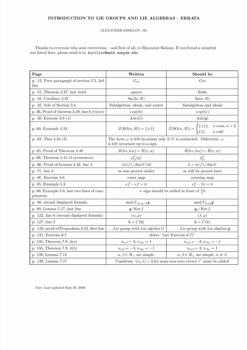
8/21/2019 Introduction to Lie Groups and Lie Algebras
http://slidepdf.com/reader/full/introduction-to-lie-groups-and-lie-algebras 235/236
INTRODUCTION TO LIE GROUPS AND LIE ALGEBRAS - ERRATA
ALEXANDER KIRILLOV, JR.
Thanks to everyone who sent corrections – and first of all, to Binyamin Balsam. If you found a misprintnot listed here, please send it to [email protected]
Page Written Should be
p. 12, First paragraph of section 2.5, 3rdline
Gm Gm
p. 15, Theorem 2.27, last word spaces fields
p. 18, Corollary 2.31 Sp(2n,K) Sp(n,K)
p. 32, title of Section 3.4 Subalgebras, ideals, and center Subalgebras and ideals
p. 36, Proof of theorem 3.29, line 6 (twice) exp(th) exp(tx)
p. 49, Exercise 3.9 (1) Aut(G) Aut(g)
p. 60, Example 4.24 Z (SO(n, R)) = {±1} Z (SO(n, R)) =
{±1}, n even, n >
{1}, n odd
p. 63, Thm 4.34 (3) The form ω is left-invariant only if G is connected. Otherwise, ωis left invariant up to a sign.
p. 65, Proof of Theorem 4.40 B(hv,hw) = B(v, w) B(hv,hw) = B(v, w)
p. 66, Theorem 4.41 (4 occurences) ρV ij(g) ρV ij
p. 66, Proof of Lemma 4.42, line 4 (tr(f )/ dim V ) id λ = tr(f )/ dim V
p. 71, line 3 as was proved earlier as will be proved later
p. 80, Exercise 4.6 cover map covering map
p. 85, Example 5.3 ef − ef = h ef − f e = h
p. 86, Example 5.6, last two lines of com-putation
+ sign should be added in front of 12
h
p. 88, second displayed formula mod U p+q−1g mod U p+qg
p. 90, Lemma 5.17, last line g/ Ker f g1/ Ker f
p. 122, line 6 (second dipslayed formula) (α, µ) (λ, µ)
p. 127, line 2 h = C (h) h = C (h)
p. 128, proof of Proposition 6.52, first line . . . Lie group with Lie algebra G . . . Lie group with Lie algebra g
p. 131, Exercise 6.7 delete “(see Exercise 6.7)”
p. 135, Theorem 7.9, 4(a) nαβ = 3, nβα = 1 nαβ = −3, nβα = −1
p. 135, Theorem 7.9, 4(b) nαβ = −3, nβα = −1 nαβ = 3, nβα = 1
p. 138, Lemma 7.15 α, β ∈ R+ are simple, α, β ∈ R+ are simple, α = β ,
p. 139, Lemma 7.17 Condition “(vi, t) > 0 for some non-zero vector t” must be added
Date : Last updated Sept 30, 2009.
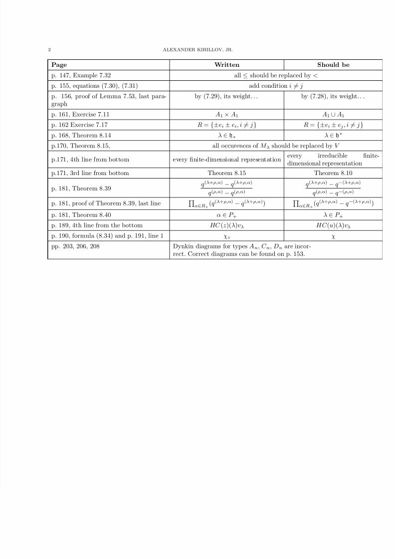
8/21/2019 Introduction to Lie Groups and Lie Algebras
http://slidepdf.com/reader/full/introduction-to-lie-groups-and-lie-algebras 236/236
2 ALEXANDER KIRILLOV, JR.
Page Written Should be
p. 147, Example 7.32 all ≤ should be replaced by <
p. 155, equations (7.30), (7.31) add condition i = j
p. 156, proof of Lemma 7.53, last para-graph
by (7.29), its weight. .. by (7.28), its weight.. .
p. 161, Exercise 7.11 A1 × A1 A1 ∪ A1
p. 162 Exercise 7.17 R = {±ei ± ei, i = j} R = {±ei ± ej , i = j}
p 168 Theorem 8 14 λ ∈ h λ ∈ h∗
Related Documents
![Lie Algebras - University of Idahobrooksr/liealgebraclass.pdf · volumes [1], Lie Groups and Lie Algebras, Chapters 1-3, [2], Lie Groups and Lie Algebras, Chapters 4-6, and [3], Lie](https://static.cupdf.com/doc/110x72/5ec51f9cde3711693f3d65c7/lie-algebras-university-of-idaho-brooksrliealgebraclasspdf-volumes-1-lie.jpg)