Introducing In-Frame Shear Constraints for Monocular …web2py.iiit.ac.in/research_centres/publications/download/...Introducing In-Frame Shear Constraints for Monocular Motion Segmentation

Introducing In-Frame Shear Constraints for Monocular MotionSegmentation

Thesis submitted in partial fulfillmentof the requirements for the degree of

MS by Researchin

Computer Science and Engineering

by

Siddharth TouraniID

[email protected]

International Institute of Information TechnologyHyderabad - 500 032, INDIA

July 2015

Copyright c© Siddharth Tourani, 2015

All Rights Reserved

International Institute of Information TechnologyHyderabad, India

CERTIFICATE

It is certified that the work contained in this thesis, titled “Introducing In-Frame Shear Constraints forMonocular Motion Segmentation” by Siddharth Tourani, has been carried out under my supervision andis not submitted elsewhere for a degree.

Date Adviser: Prof. K Madhava Krishna

.

Acknowledgments

In chronological order.1) My Parents2) Mr. K K Kumar3) Dr. Gaurav Dar4) Dr. Jayanti Sivaswamy5) Dr. K Madhava Krishna6) Labmates7) RSP, Arp-Ray and Tejas.

v

Abstract

In this thesis, the problem of motion segmentation is discussed. The aim of motion segmentation isto decompose a video into different objects that move through the sequence. In many computer visionpipelines, this is an important, middle step. It is essential in several applications like robotics, visualsurveillance and traffic monitoring. While,there is already a vast amount of literature on the topic, theperformance of all thus-far proposed algorithms are far behind human perception.

This thesis starts of with a formal introduction to the problem. Then, it proceeds to explain themain approaches proposed to the problem, along with their advantages, and shortcomings. Finally, theproposed algorithm, that forms the keystone of this thesis, is introduced and fully-fleshed out, givingmotivation for the structure and the various parts of the algorithm. In addition, the traditional comparisonis given with the other-proposed state-of-the art algorithms. We do so, on the standard benchmarkHopkins-155 dataset, as well as a new dataset, compiled from video sequences from the publicallyavailable, KITTI dataset, the Versailles-Rond sequence taken from [] and several sequences taken aroundthe IIIT Hyderabad campus. The sequences in the dataset, consist of video footage taken from a single-camera mounted on the front of a car. The dataset is far more realistic and challenging than the Hopkinsdataset, and provides a more rigorous assessment for both the proposed algorithm, as well as otherstate-of-the-art algorithms in motion segmentation. This dataset is hereby referred to as the On-Roaddataset.

On the Hopkins-155, our algorithm achieves near state-of-the-art performance, while performingsubstantially better on the On-Road dataset, showing that the proposed algorithm, has superior perfor-mance in realistic scenarios.

vi

Contents

Chapter Page

1 Introduction . . . . . . . . . . . . . . . . . . . . . . . . . . . . . . . . . . . . . . . . . . 11.1 Two Main Approaches To Motion Segmentation . . . . . . . . . . . . . . . . . . . . . 3

1.1.1 Matrix Factorization . . . . . . . . . . . . . . . . . . . . . . . . . . . . . . . 31.1.2 Multibody Extension . . . . . . . . . . . . . . . . . . . . . . . . . . . . . . . 41.1.3 Gestalt Based Segmentation . . . . . . . . . . . . . . . . . . . . . . . . . . . 61.1.4 Discussion . . . . . . . . . . . . . . . . . . . . . . . . . . . . . . . . . . . . 7

1.2 Datasets Used . . . . . . . . . . . . . . . . . . . . . . . . . . . . . . . . . . . . . . . 71.2.1 Hopkins-155 Dataset . . . . . . . . . . . . . . . . . . . . . . . . . . . . . . . 71.2.2 On-Road Dataset . . . . . . . . . . . . . . . . . . . . . . . . . . . . . . . . . 8

1.3 Objective of thesis and Design Principles underlying the proposed motion segmentationalgorithm. . . . . . . . . . . . . . . . . . . . . . . . . . . . . . . . . . . . . . . . . . 81.3.1 Objectives . . . . . . . . . . . . . . . . . . . . . . . . . . . . . . . . . . . . . 81.3.2 Design Principles . . . . . . . . . . . . . . . . . . . . . . . . . . . . . . . . . 8

1.4 Thesis Overview . . . . . . . . . . . . . . . . . . . . . . . . . . . . . . . . . . . . . 9

2 Related Works . . . . . . . . . . . . . . . . . . . . . . . . . . . . . . . . . . . . . . . . . 102.1 Frame Differencing . . . . . . . . . . . . . . . . . . . . . . . . . . . . . . . . . . . . 102.2 Epipolar Geometry Based . . . . . . . . . . . . . . . . . . . . . . . . . . . . . . . . . 112.3 Optical Flow /Gestalt Based . . . . . . . . . . . . . . . . . . . . . . . . . . . . . . . 132.4 Layers . . . . . . . . . . . . . . . . . . . . . . . . . . . . . . . . . . . . . . . . . . . 152.5 Subspace Clustering Based . . . . . . . . . . . . . . . . . . . . . . . . . . . . . . . . 16

3 Proposed Algorithm . . . . . . . . . . . . . . . . . . . . . . . . . . . . . . . . . . . . . . 193.0.1 Initial Foreground-Background Segmentation . . . . . . . . . . . . . . . . . . 203.0.2 Biased Affine Motion Model Sampling . . . . . . . . . . . . . . . . . . . . . 213.0.3 Initial Assignment of the Unsampled Points . . . . . . . . . . . . . . . . . . . 223.0.4 Segmentation Refinement by Energy-Minimization . . . . . . . . . . . . . . . 24

3.1 Model Selection . . . . . . . . . . . . . . . . . . . . . . . . . . . . . . . . . . . . . . 263.1.1 Model Merging Predicate . . . . . . . . . . . . . . . . . . . . . . . . . . . . 29

4 Results . . . . . . . . . . . . . . . . . . . . . . . . . . . . . . . . . . . . . . . . . . . . . 304.1 Hopkins-155 Results . . . . . . . . . . . . . . . . . . . . . . . . . . . . . . . . . . . 304.2 On-Road Dataset . . . . . . . . . . . . . . . . . . . . . . . . . . . . . . . . . . . . . 33

5 Conclusions . . . . . . . . . . . . . . . . . . . . . . . . . . . . . . . . . . . . . . . . . . 37

vii

viii CONTENTS

Bibliography . . . . . . . . . . . . . . . . . . . . . . . . . . . . . . . . . . . . . . . . . . . . 39

List of Figures

Figure Page

1.1 The two main approaches to point tracking. . . . . . . . . . . . . . . . . . . . . . . . 21.2 Interpretation of the Trajcectory Matrix . . . . . . . . . . . . . . . . . . . . . . . . . 31.3 Factorization of trajectory matrix W into motion matrix M and structure matrix S. . . . 41.4 Multibody Factorization of the trajectory matrix . . . . . . . . . . . . . . . . . . . . . 51.5 Patterns classified by Subspace Clustering Algorithms. (a) is taken from 77. (b) is taken

from 26. (c) is taken from 26. . . . . . . . . . . . . . . . . . . . . . . . . . . . . . . 6

2.1 Illustration of how the epipolar constraint functions and fails. In (a) the 3d-point P onmoving to P’ off the epipolar plane is projected into the primed camera frame C’ abovethe epipolar line l’. In (b) P’ still lies on the epipolar plane and is projected right ontothe l’. In (b) the epipolar constraint cannot be used to detect P’ as moving. . . . . . . 12

3.1 An Overview of the Proposed Approach . . . . . . . . . . . . . . . . . . . . . . . . . 203.2 Figure shows a result of the initial foreground-background segmentation. The fore-

ground (epipolar outliers) are shown in blue, and background (epipolar inliers) areshown in red. (a) In the non-degenerate case most, of the points on the moving ve-hicle have been categorized as not belonging to the background. (b) In the degeneratecase, most of the points on the vehicle belong to the background. . . . . . . . . . . . . 21

3.3 Difference between minimum residual and Top-k residual sampling. . . . . . . . . . . 243.4 Results from the Hopkins-155 dataset.The various stages of our proposed approach are

shown. The tracked points shown in the figure were not the ones used to verify theaccuracy of our approach on the Hopkins-155 dataset. These are shown here primarilyfor illustrative purposes. . . . . . . . . . . . . . . . . . . . . . . . . . . . . . . . . . 25

3.5 Illustration of how shear and stretch work. Top row: The case where models are detectedas seperate. In (a) and (b) the initial and final frames are shown along with two motionmodels. The notion of shear being clearly visible. In (c) is shown the cumulative shearvs number of frames plot. Likewise in (d), but for stretch. Bottom row: The case weremodels are merged are shown in the bottom row with symmetric plots. . . . . . . . . 28

4.1 Error Distribution Histogram for the Hopkins-155 Dataset . . . . . . . . . . . . . . . 324.2 Percentage Accuracy With Gaussian Noise Added To The Trajectory Data. . . . . . . . 324.3 Box-plot assessing the performancce of various algorithms at estimating the number of

motions. . . . . . . . . . . . . . . . . . . . . . . . . . . . . . . . . . . . . . . . . . . 334.4 Comparison of various state-of-the-art motion segmentation algorithms for the On-Road

Dataset. . . . . . . . . . . . . . . . . . . . . . . . . . . . . . . . . . . . . . . . . . . 34

ix

List of Tables

Table Page

4.1 Total Error Rates in Noise-Free Case. The first row represents error rates for all (155seqeunces). The second and third rows are two and three motions, respectively. Thevalues of the algorithms were taken from their corresponding papers. . . . . . . . . . . 31

4.2 Total Computation Time on the Hopkins-155 Dataset in seconds. . . . . . . . . . . . . 314.3 Error Rates on the On-Road Dataset For the various sequences. Error Rates for the

various algorithms under consideration . . . . . . . . . . . . . . . . . . . . . . . . . . 35

x

Chapter 1

Introduction

This chapter starts off by introducing the motion segmentation problem. The two main approaches tothe motion segmentation problem are explained in Section 1.1. The datasets on which our experimentswere conducted on are introduced in Section 1.2. The objective of this thesis, along with the motivationand design principles behind the proposed algorithm, are provided in Section 1.3. Finally, the structureof the thesis is described in Section 1.4

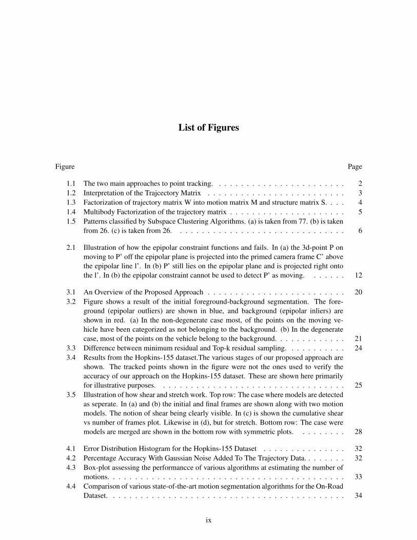
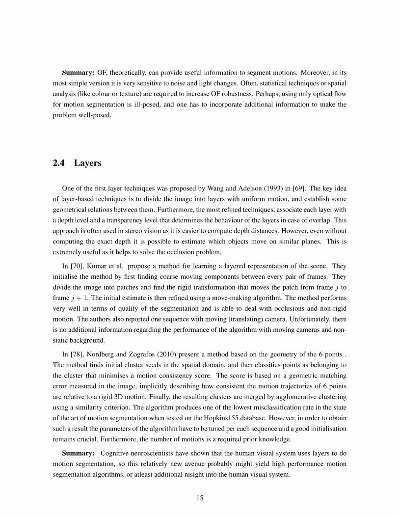
The problem of motion segmentation consists of segmenting out the regions in the video correspond-ing to different motions and background. Generally, as input a motion segmentation algorithm receivesin one form or another the set of tracked points, over a number of frames. These tracked points are theoutput of a standard-of-the shelf tracking algorithm. The points are tracked using either a dense-featuretracker, or a sparse-feature based tracker. Dense-Feature trackers aim at tracking every single pixel inthe image, when compared to sparse-feature based trackers, which track a smaller number of points,which are more ”visually” salient in a certain mathematical sense (please refer to [51] for details) andtherefore, more easily trackable. Dense tracking comes at a higher computational cost, than sparsetracking, making it unsuitable atleast given current computational constraints, for robotic (usually real-time) use. In this thesis, we restrict our use to sparse features for one other reason. The Hopkins dataset[27], which has since the year 2007, served as a benchmark for evaluating the performance of all motionsegmentation algorithms, provides for testing, a sparse set of feature trajectory points, generally num-bering between 100 and 600 depending on the sequence. However, this does not mean that the proposedalgorithm does not work on dense trajectories. In whatever informal evaluation we have done on densetrajectories, both in terms of speed and classification accuracy, our algorithm, improves in performancerelative to the state-of-the-art.

Fig. (1.1). a shows the result of motion segmentation, on a dense tracking algorithm. Fig (b) showsthe result of motion segmentation on a sparse tracking algorithm.

For uniformity, from henceforth, throughout the thesis the number of points tracked is denoted by Pand number of frames over which the video was tracked by F.

The feature tracke we use in this thesis the the Kanade-Lucas-Tomsi (KLT) tracker. The output ofthis tracker, is a set of P pixel values tracked over all F frames. The typical structure used to represent

1

(a) Motion Segmentation after dense tracking (b) Motion Segmentation after sparse tracking

Figure 1.1: The two main approaches to point tracking.

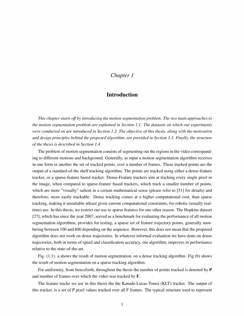
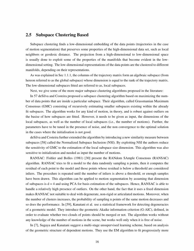
these tracked points is in the form of a 2F × P matrix called the trajectory matrix, hereby denoted asW.

W =

x1,1 . . . x1,P

y1,1 . . . y1,P

.... . .

...xF,1 . . . xF,P

yF,1 . . . yF,P

(1.1)

xi,j , yi,j represents the x and y image co-ordinates of the jth tracked point in the ith frame. Therefore,each column in the W matrix represents the entire trajectory of a particular tracked point. Every tworows of the same i-index correspond to the set of all tracked points in a certain frame, as shown in Fig.[1.2].

A common assumption made by most motion segmentation algorithms, is that the camera modelis orthographic/affine instead of perspective, eventhough perspective camera models are closer to re-ality than affine cameras. This simplification allows a mathematical solution that is easily tractable asexplained in Section 1.1.

The orthographic camera model, is valid only when the rays captures by the camera hit the imageplane perpendicularly. This holds roughly true, when the objects are far off, but is a poor estimate whenthe objects are close-by.

The motion segmentation problem can thus be framed as partitioning the columns of W matrix into(n + 1)-groups, where n is the number of moving objects in the scene and the additional one is for thebackground.

2

Figure 1.2: Interpretation of the Trajcectory Matrix

Several philosophies, and design principles have been proposed to solve this problem. We review inthe next section the two main approaches. The section provides a broad overview of the approaches.Specific algorithms, their strengths and weaknesses are discussed in the next chapter.

1.1 Two Main Approaches To Motion Segmentation

Broadly, the two approaches to motion segmentation, are,

• Matrix Factorization: These approaches involve factorizing W in such a way that the indepen-dent motions pop out, based on mathematically rigorous rank constraints for W.

• Gestalt Based Segmentation: These approaches are perceptually-inspired, by the principle of”common fate” or gestalt 18, and use similarity metrics between trajectories (columns of W) todetect dominant motions.

1.1.1 Matrix Factorization

In this section, we review the geometry of the 3-D motion segmentation problem from multipleaffine views and show that it is equivalent to clustering multiple low-dimensional linear subspaces of ahigh-dimensional space.

Let {xf ∈ R2}f=1,...,Fp=1,...,P be the projections of P 3-D points {Xp ∈ P3}Pp=1 lying on a rigidly moving

object onto F frames of a rigidly moving camera. Under the affine projection model, which generalizesorthographic, weak perspective and paraperspective projection, the images staisfy the equation

xfp = AfXp (1.2)

whereis the affine camera matrix at frame f , which depends on the camera calibration parameters Kf ∈

R2×3 and the object pose relative to the camera (Rt, tf ) ∈ SE(3).

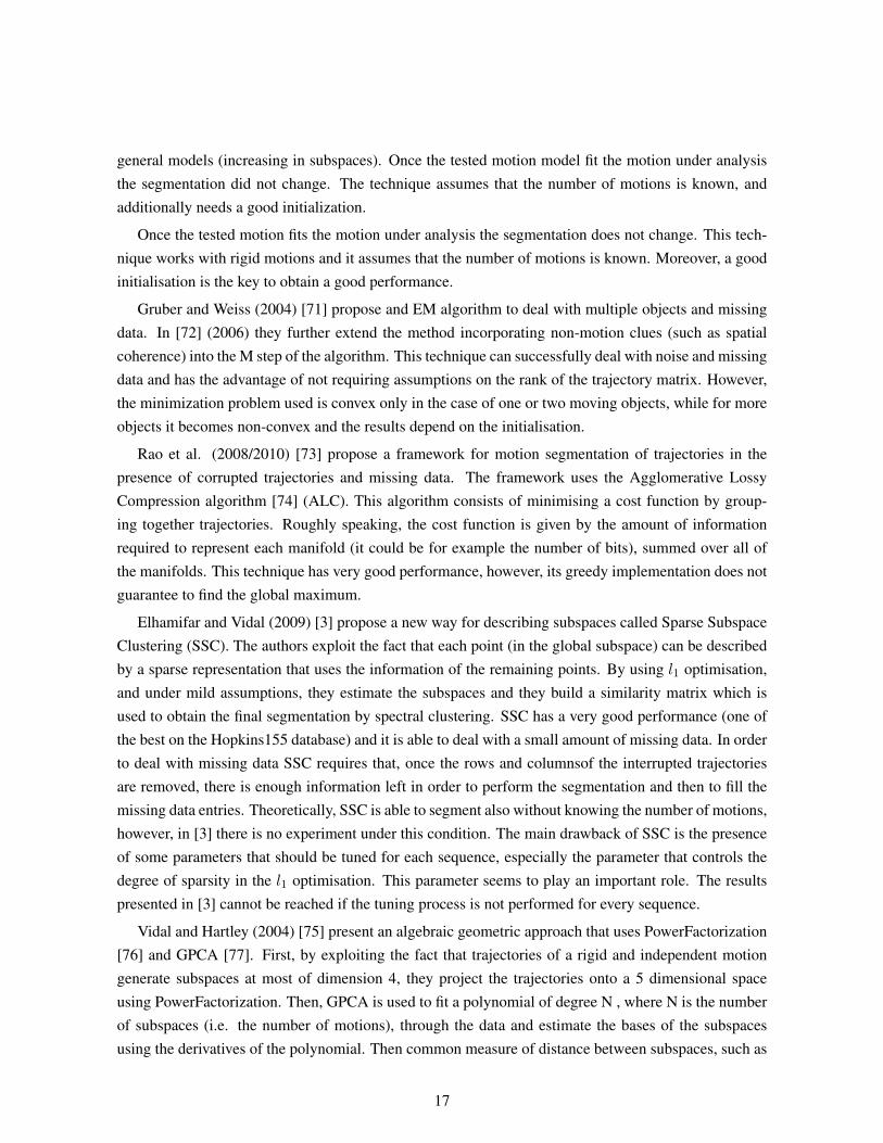
W1 = M1ST1 (1.3)

3

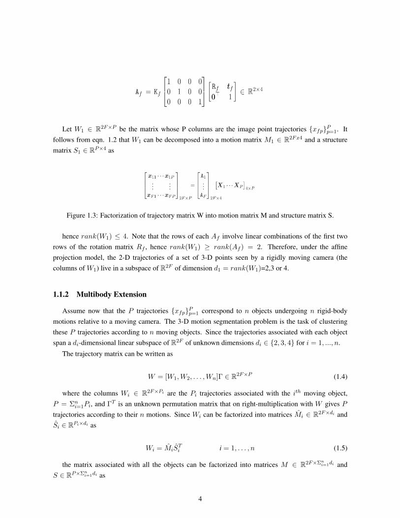
Let W1 ∈ R2F×P be the matrix whose P columns are the image point trajectories {xfp}Pp=1. Itfollows from eqn. 1.2 that W1 can be decomposed into a motion matrix M1 ∈ R2Fx4 and a structurematrix S1 ∈ RP×4 as

Figure 1.3: Factorization of trajectory matrix W into motion matrix M and structure matrix S.

hence rank(W1) ≤ 4. Note that the rows of each Af involve linear combinations of the first tworows of the rotation matrix Rf , hence rank(W1) ≥ rank(Af ) = 2. Therefore, under the affineprojection model, the 2-D trajectories of a set of 3-D points seen by a rigidly moving camera (thecolumns of W1) live in a subspace of R2F of dimension d1 = rank(W1)=2,3 or 4.

1.1.2 Multibody Extension

Assume now that the P trajectories {xfp}Pp=1 correspond to n objects undergoing n rigid-bodymotions relative to a moving camera. The 3-D motion segmentation problem is the task of clusteringthese P trajectories according to n moving objects. Since the trajectories associated with each objectspan a di-dimensional linear subspace of R2F of unknown dimensions di ∈ {2, 3, 4} for i = 1, ..., n.

The trajectory matrix can be written as

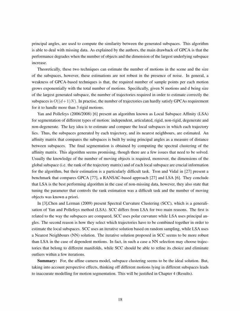
W = [W1,W2, . . . ,Wn]Γ ∈ R2F×P (1.4)

where the columns Wi ∈ R2F×Pi are the Pi trajectories associated with the ith moving object,P = Σn

i=1Pi, and ΓT is an unknown permutation matrix that on right-multiplication with W gives Ptrajectories according to their n motions. Since Wi can be factorized into matrices Mi ∈ R2F×di andSi ∈ RPi×di as

Wi = MiSTi i = 1, . . . , n (1.5)

the matrix associated with all the objects can be factorized into matrices M ∈ R2F×Σni=1di and

S ∈ RP×Σni=1di as

4

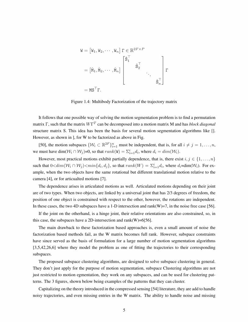
Figure 1.4: Multibody Factorization of the trajectory matrix

It follows that one possible way of solving the motion segmentation problem is to find a permutationmatrix Γ, such that the matrix WΓT can be decomposed into a motion matrix M and has block diagonalstructure matrix S. This idea has been the basis for several motion segmentation algorithms like [].However, as shown in ], for W to be factorized as above in Fig.

[50], the motion subspaces {Wi ⊂ R2F }ni=1 must be independent, that is, for all i 6= j = 1, . . . , n,we must have dim(Wi ∩Wj)=0, so that rank(W) = Σi

i=1di, where di = dim(Wi).

However, most practical motions exhibit partially dependence, that is, there exist i, j ∈ {1, . . . , n}such that 0<dim(Wi ∩ Wj)<min{di, dj}, so that rank(W ) = Σi

i=1di, where di=dim(Wi). For ex-ample, when the two objects have the same rotational but different translational motion relative to thecamera [4], or for articualted motions [7].

The dependence arises in articulated motions as well. Articulated motions depending on their jointare of two types. When two objects, are linked by a universal joint that has 2/3 degrees of freedom, theposition of one object is constrained with respect to the other, however, the rotations are independent.In these cases, the two 4D subspaces have a 1-D intersection and rank(W)=7, in the noise free case [56].

If the joint on the otherhand, is a hinge joint, their relative orientations are also constrained, so, inthis case, the subspaces have a 2D-intersection and rank(W)=6[56].

The main drawback to these factorization based approaches is, even a small amount of noise thefactorization based methods fail, as the W matrix becomes full rank. However, subspace constraintshave since served as the basis of formulation for a large number of motion segmentation algorithms[3,5,42,26,6] where they model the problem as one of fitting the trajectories to their correspondingsubspaces.

The proposed subspace clustering algorithms, are designed to solve subspace clustering in general.They don’t just apply for the purpose of motion segmentation, subspace Clustering algorithms are notjust restricted to motion egmentation, they work on any subspaces, and can be used for clustering pat-terns. The 3 figures, shown below being examples of the patterns that they can cluster.

Capitalizing on the theory introduced in the compressed sensing [54] literature, they are add to handlenoisy trajectories, and even missing entries in the W matrix. The ability to handle noise and missing

5

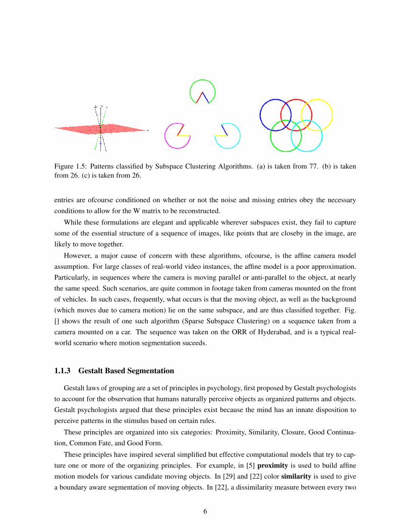
Figure 1.5: Patterns classified by Subspace Clustering Algorithms. (a) is taken from 77. (b) is takenfrom 26. (c) is taken from 26.

entries are ofcourse conditioned on whether or not the noise and missing entries obey the necessaryconditions to allow for the W matrix to be reconstructed.

While these formulations are elegant and applicable wherever subspaces exist, they fail to capturesome of the essential structure of a sequence of images, like points that are closeby in the image, arelikely to move together.

However, a major cause of concern with these algorithms, ofcourse, is the affine camera modelassumption. For large classes of real-world video instances, the affine model is a poor approximation.Particularly, in sequences where the camera is moving parallel or anti-parallel to the object, at nearlythe same speed. Such scenarios, are quite common in footage taken from cameras mounted on the frontof vehicles. In such cases, frequently, what occurs is that the moving object, as well as the background(which moves due to camera motion) lie on the same subspace, and are thus classified together. Fig.[] shows the result of one such algorithm (Sparse Subspace Clustering) on a sequence taken from acamera mounted on a car. The sequence was taken on the ORR of Hyderabad, and is a typical real-world scenario where motion segmentation suceeds.

1.1.3 Gestalt Based Segmentation

Gestalt laws of grouping are a set of principles in psychology, first proposed by Gestalt psychologiststo account for the observation that humans naturally perceive objects as organized patterns and objects.Gestalt psychologists argued that these principles exist because the mind has an innate disposition toperceive patterns in the stimulus based on certain rules.

These principles are organized into six categories: Proximity, Similarity, Closure, Good Continua-tion, Common Fate, and Good Form.

These principles have inspired several simplified but effective computational models that try to cap-ture one or more of the organizing principles. For example, in [5] proximity is used to build affinemotion models for various candidate moving objects. In [29] and [22] color similarity is used to givea boundary aware segmentation of moving objects. In [22], a dissimilarity measure between every two

6

point trajectories is computed, on the basis of which spectral clustering is done. The formulation of thedissimilarity measure, is on the basis of gestalt principles.

The general framework of such algorithms is that, between two or more trajectories, that is thecolumns of W, a dissimilarity measure is computed, which is spectrally projected and clustered using astandard/accelerated k-means algorithm.

1.1.4 Discussion

The two methods, have been effective in dealing with video sequences, where the camera motionis as such sufficiently different from the moving objects, to allow for the theory of affine subspaces tocome into play. The sequences also had sufficient flow differences between the background and themoving objects, to allow for a convenient dissimilarity measure between background and moving objectto be defined.

However, when we tested, the state-of-the-art algorithms from both categories, on datasets, wherethe camera is moving and the moving object and camera have same direction of motion, the algorithmsfailed quite often.

In the case of a moving camera, seperating stationary objects from non-stationary ones, is ratherchallenging, as the camera motion causes most of the pixels to move. The apparent motion of points, isa combined effect of camera motion, object depth and perspective effects and noise.

Optical flow vectors for nearby stationary objects may have a larger magnitude, than those for far-away objects that are in motion, thus one cannot exclusively use optical flow as the basis for a motionsegmentation algorithm. Likewise, the geometric constraints imposed by epipolar geometry [15], do nothold for the same relative motion configurations between the camera and the moving object.

Another drawback of most of these methods, is that they require the number of moving objects inthe scene to be known beforehand, which is an unrealistic assumption for most real-world applications.

1.2 Datasets Used

We show results on two main datasets. The first is the Hopkins-155 [27] dataset benchmark intro-duced in 2007 and a dataset consisting of sequences taken from a camera mounted in front of a movingcar. The dataset consists of sequences taken from the KITTI dataset [21], [17] and sequences takenclose to IIIT Hyderabad.

1.2.1 Hopkins-155 Dataset

The Hopkins 155-dataset consists of 155 video sequences, of which 120 consist of two moving ob-jects and 35 consist of three moving objects. The sequences are divided into three categories, checker-board, traffic and articulated. There are a total of 104 checkerboard sequences, 38 traffic sequencesand 13 articulated sequences. The sequences consist have 100-600 tracked points per sequence. The

7

sequences are taken by a hand-held camera. The very high accuracy achieved by subspace clusteringalgorithms indicate that the affine camera model, is a good approximation for these sequences.

1.2.2 On-Road Dataset

The On-Road dataset, consists of 7 sequences encountered in an autonomous vehicles setting. Thecamera in all of the sequences is mounted on the front of the vehicle. The sequences are chosen be-cause, they come close to the case of degenerate / dependent motion, and are much closer to real-worldscenarios.

1.3 Objective of thesis and Design Principles underlying the proposed

motion segmentation algorithm.

1.3.1 Objectives

In this thesis, we develop a motion segmentation algorithm, capable of handling real-world de-generate motion scenarios, while having backward compatibility. i.e, we want the algorithm to not bespecailized to deal with only the degenerate motion case, but rather all real-world motions.

For the algorithm to be used in real-time robotic systems, it has to be fast. In addition, it has to beable to do so, without any prior knowledge of the number of moving objects.

Additionally, the method should be robust to outliers and noisy trajectory information.

1.3.2 Design Principles

In design of the proposed motion segmentation algorithm, we have incorporated other relative motioncues, that capture the difference/similarity in motion between multiple objects. We use notions of motionsimilarity based on:

• Common Fate: Points tracked on an object should move similarly.

• Temporal Consistency: The above similarity should hold over time as well.

• Local Spatial Coherence: Points sampled from a small region should have similar motion.

to design our motion segmentation algorithm, in addition to the standard geometric ones. The aboveprinciples are quite general, and do not make any strong assumptions about either the scene, cameramodel or motion between objects.

8

1.4 Thesis Overview

The remainder of this thesis is organized as follows. In Chapter 2, we survey the general methodsrelated to motion segmentation, presenring their strengths and weaknesses. In Chapter 3, we presentour algorithm, with intermediate results, of the algorithm’s proposed pipeline. In Chapter 4, we presentthe results of our algorithm and comparison with other methods. In Chapter 5, we conclude along withpossible future directions of research.

9

Chapter 2

Related Works

In this chapter, the major approaches to the problem of motion segmentation are summarized. Thisis done, not only for the two main classes discussed in Sec1.1, but also others. However, we focus moreon subspace clustering and gestalt inspired algorithms as theyu have proven to be the most accurateand versatile approaches.

Motion Segmentation has been researched for nearly 25 years, by researchers in computer visionand cognitive psychology, so the literature is quite rich and voluminous. In order, to make the overviewsystematic, we divide the approaches into different categories, on the basis of the underlying principleof the motion segmentation algorithm. The division, is not strict. Some algorithms belong to more thanone group.

The classes are:

• Frame Differencing Based

• Epipolar Geometry Based

• Optical Flow / Gestalt Based

• Layer Based

• Subspace Clustering Based

A table summarizing the different vital statistics about the algorithm is shown below

2.1 Frame Differencing

Frame differencing techniques, are some of the oldest and simplest techniques for motion segmen-tation. They are often used in settings where the camera is fixed, and is viewing a generally staticenvironment. It is used in intrusion detection systems and intelligent power sensors, to detect the pres-ence/absence of people. These methods consist of applying a simple threshold to the pixel-value inten-sities, and only works when most of the background is static and camera has zero motion.

10

In [60], Cavallaro uses a probability based test in order to set the threshold locally in the image, re-inforcing the motion differencing over several frames. This first step allows a coarse map of the movingobjects. Each blob is then decomposed into non-overlapping regions. From each region spatial and tem-poral features are extracted. This technique is capable of dealing with multiple objects, occlusions andnon-rigid objects. Unfortunately, the region segmentation stage is based on an iterative process whichmakes the algorithm time consuming. Another limitation is due to the initialisation performed when agroup of objects enter in the scene, in such cases the algorithm assigns them a unique label rather thantreating them as separated objects.

In [61], perform image differencing on the low-frequency sub-image of the third level of a discretewavelet transform. On the extracted blobs they perform some morphological operations and extract thecolour and spatial information. In this way each blob is associated with a descriptor that is used to trackthe objects throughout the sequence. no motion compensation or statistical background is built whichmakes the method not suitable for moving camera applications.

In [62], Li et al. use image difference in order to localise moving objects. The noise problem is atten-uated by decomposing the image in non-overlapping blocks and working on its average intensity value.They also use an inertia compensation to avoid loosing tracked objects when the objects temporarilystop. This technique deals successfully with the temporary stopping problem, but its main drawbacksare the high number of parameters that require tuning and the inability to deal with moving cameras.

In [63], Colombari et al. propose a robust statistic to model the background. For each frame a mosaicof the background is back-warped onto the frame. A binary image that indicates for each pixel whether itbelongs to a moving object or not is obtained. Then, the binary image is cleaned and regions are mergedand define blobs. By exploiting temporal coherence the blobs are tracked throughout the sequence. Thistechnique is able to deal with occlusions, appearing and disappearing objects. The background mosaicis done off-line and in order to recover the motion of the camera it is necessary to extract many featuresin the non-moving area.

Summary Frame differencing algorithms are still very sensitive to noise and to light changes, hence,they cannot be considered an ideal choice in the case of a cluttered or moving background. Framedifference alone cannot perform segmentation, it is only able to detect motions.

2.2 Epipolar Geometry Based

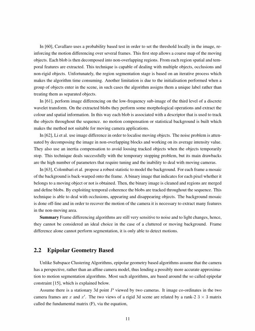
Unlike Subspace Clustering Algorithms, epipolar geometry based algorithms assume that the camerahas a perspective, rather than an affine camera model, thus lending a possibly more accurate approxima-tion to motion segmentation algorithms. Most such algorithms, are based around the so called epipolarconstraint [15], which is explained below.

Assume there is a stationary 3d point P viewed by two cameras. It image co-ordinates in the twocamera frames are x and x′. The two views of a rigid 3d scene are related by a rank-2 3 × 3 matrixcalled the fundamental matrix (F), via the equation,

11

(a) Point Off Epipolar Plane (b) Point On Epipolar Plane

Figure 2.1: Illustration of how the epipolar constraint functions and fails. In (a) the 3d-point P onmoving to P’ off the epipolar plane is projected into the primed camera frame C’ above the epipolar linel’. In (b) P’ still lies on the epipolar plane and is projected right onto the l’. In (b) the epipolar constraintcannot be used to detect P’ as moving.

x′TFx = 0 (2.1)

The plane defined by the camera centres of the two views and the 3-D point is called the epipolarplane. On the basis, of whether a point lies on the epipolar plane or not, the motion segmentation canbe done as follows.

Assume , that the point P has moved to P ′. x and x′ are 2d-image co-ordinates of a 3d pixel viewedfrom two views. Geometrically Fx represents the epipolar line in l′ in the primed view co-ordinatesystem. If the 3d point P corresponding to x and x′ are stationary, then in the case of zero-noise |l′x′|=0holds.

This constraint, known as the epipolar constraint, can be used to distinguish between moving andstationary points, in most cases. Fig (2.1). a shows a typical case where the point P has moved to P ′ itsprojection in the second image x′ lies above the line l′.

However, if P were moving in on the epipolar plane itself, as in Fig (2.1).b such that it’s imagelies on the epipolar line, yielding a zero value for epipolar constraint. Such a configuration is called adegenerate configuration, and it corresponds to the degenerate configuration for the affine camera.

These degenerate configurations arise when the camera and object motion are either parallel or anti-parallel, and there is no rotation between two camera scenes. The epipolar constraint fails for thesedegenerate scenarios. In the case of autonomous vehicles, one can argue that these situations, are morecommon than the non-degenerate case, which will occur mostly at road intersections.

Having sufficient background in epipolar geometry, we can proceed to review the epipolar geometrybased algorithms.

In [24], Kundu et al., combined the epipolar constraint along with optical flow information in a Bayesfilter, based framework to detect motion segmentation. To deal with the degenerate case, in [24] et al.proposed a new motion segmentation constraint called the flow-vector bound (FVB) constraint whichprovided a mathematically accurate model of the degenerate case, as follows,

12

x′ = x+Kt

z(2.2)

Here, x and x′ are the image co-ordinates at two time instances. K is the calibration matrix. t is therelative translation, z is the depth of the 3d point in question in the non-primed co-ordinate frame.

The problem with their method, is estimating z and t is quite challenging, in their paper they useinformation from an Inertial Measurement Unit and are thus able to get an accurate estimate. However,all the sequences for which they tested for, were indoor on a flat floor allowing the IMU to give a goodsensor reading. For, outdoor scenarios, the IMU estimate would be much noisier. Nieto. et al. used theirstereo system to compute the t and z and, were able to report reasonable results using the

Both the systems rely on sensors that are able to give reasonably accurate estimates of t and z. This,would be far more challenging for case of monocular camera without any additional sensor information.

In [1], Namdev et.al. computed the t and z for the FVB constraint using a monocluar V-SLAMsystem running in the backend. Monocular V-SLAM systems are known to be inherently noisy andtend to break easily even as this thesis was written, thus leading to suspect results, especially given theirexceptionally high quality.

Summary While the constraints model the motion segmentation problem with the highest accuracy,they require unreasonably accurate estimation of the relative rotation and translation between two cam-era frames and depth of the 3d point corresponding to the pixel values. This may not be possible withoutincorporating high end sensors, making the methods unfeasible atleast for the present.

2.3 Optical Flow /Gestalt Based

Optical flow (OF) is the distribution of apparent velocities in an image sequence. By apparent, wemean it needs to be seen in the image. If an object is moving in the image sequence, but, is far away,it apparent movement in the image space (it’s optical flow) will be much lesser than a close by objecteven if the closer by object has a much smaller velocity in the 3D world, than the object farther away.

Optical flow was computed for image sequences by Horn and Schunk in 1980 [64]. The basic ideabehind OF algorithms is to use discontinuities in the OF in order to segment moving objects. In fact,there was a list of methods proposed for motion segmentation, before the first OF algorithm was feasibleto run on a computer system.

Since the work of Horn and Schunck, many other approaches have been proposed. In the past,the main limitations of such methods were high sensitivity to noise and expensive computational cost.Nowadays, thanks to the high process speed of computers and to improvements made by research, OFis widely used.

The fact that motion provides important information for grouping is well known and dates back toKoffka and Wertheimer suggesting the Gestalt principle of common fate [18]. Various approaches havebeen proposed for taking this grouping principle into account.

13

In [65], Trucco et al. merge image difference with OF. Specifically, they propose to estimate theOF only at pixels where motion is significant. The image difference is responsible for identification ofareas where significant motion occurs. The map produced by the image difference is called in the paperdisturbance field and is computed as the difference between the current frame and an exponentially-weighted average of the past frames. The OF is based on a recursive-filter formulation. This techniqueassumes that flow is smooth and changes slowly over time. Thanks to the fact that the OF is computedonly when it is necessary the algorithm is faster than most of OF-based solutions.

In [66], Zhang et al. propose a method to segment multiple rigid-body motions using Line OF. Incontrast to classical OF algorithms (which are based on points), the line OF algorithm can work alsowhen the moving object has a homogeneous surface, provided that the object edges can be identifiedand used as pieces of straight lines. The limitation of this method is that it is not able to deal with non-rigid motions because it requires straight lines in order to compute the OF. This approach uses K-meansin order to build the final clusters, hence, it also assumes that the number of moving objects (i.e. thenumber K of clusters) is known a priori.

In [67], Xu et al. propose a variational formulation of OF combined with colour segmentationobtained by the Mean-Shift [68] algorithm. Moreover, in order to deal with non-rigidity a confidencemap is built to measure the confidence of whether the segmentation and the corresponding motion modelsuit the flow estimation or not. This technique is also able to deal with partial occlusions.

In [22],Brox and Malik propose to compute a dense OF field and extract measures of similaritybetween each pair of trajectories. The similarity involves Euclidean distances between trajectories ingiven windows of time and the average flow variation of the local field (as a negative contribution tothe similarity). The authors also propose a spectral clustering method that includes a spatial regularityconstraint. By exploiting such a regularity constraints the algorithm is able to estimate the number ofclusters in the scene by model selection. The results presented in this work show accurate segmentations.However, the fact that the algorithm relies on 2D image spatial distances may create some problemswhen dealing with non-rigid motions. Furthermore, as a consequence of the use of 2D image distances,it seems that the algorithm requires long sequences in order to be able to perform the segmentationaccurately. In fact, if two object are close and they undergo two different, but not long, motions they arelikely to be given a high similarity and, therefore, be clustered as the same object.

In [29], Katrina et al. like Brox and Malik computed a similarity measure between two trajectories,which she then clustered using a normalized cut algorithm. She modified the Laplacian matrix to down-weigh the nodes that frequently change neighbors in the Delaunay Triangulation of the scene. This wasdone on the basis that the neighbors of moving objects change when compared to stationary objects.In spirit, this method is probably closest to our proposed approach, in that it exploits the change inspatial relations at the interface of an image. When testing on our datasets was that, there was a slightoversegmentation of the scene, and the method would have had strong performance, if followed by anadditional model merging step.

14

Summary: OF, theoretically, can provide useful information to segment motions. Moreover, in itsmost simple version it is very sensitive to noise and light changes. Often, statistical techniques or spatialanalysis (like colour or texture) are required to increase OF robustness. Perhaps, using only optical flowfor motion segmentation is ill-posed, and one has to incorporate additional information to make theproblem well-posed.

2.4 Layers

One of the first layer techniques was proposed by Wang and Adelson (1993) in [69]. The key ideaof layer-based techniques is to divide the image into layers with uniform motion, and establish somegeometrical relations between them. Furthermore, the most refined techniques, associate each layer witha depth level and a transparency level that determines the behaviour of the layers in case of overlap. Thisapproach is often used in stereo vision as it is easier to compute depth distances. However, even withoutcomputing the exact depth it is possible to estimate which objects move on similar planes. This isextremely useful as it helps to solve the occlusion problem.

In [70], Kumar et al. propose a method for learning a layered representation of the scene. Theyinitialise the method by first finding coarse moving components between every pair of frames. Theydivide the image into patches and find the rigid transformation that moves the patch from frame j toframe j + 1. The initial estimate is then refined using a move-making algorithm. The method performsvery well in terms of quality of the segmentation and is able to deal with occlusions and non-rigidmotion. The authors also reported one sequence with moving (translating) camera. Unfortunately, thereis no additional information regarding the performance of the algorithm with moving cameras and non-static background.

In [78], Nordberg and Zografos (2010) present a method based on the geometry of the 6 points .The method finds initial cluster seeds in the spatial domain, and then classifies points as belonging tothe cluster that minimises a motion consistency score. The score is based on a geometric matchingerror measured in the image, implicitly describing how consistent the motion trajectories of 6 pointsare relative to a rigid 3D motion. Finally, the resulting clusters are merged by agglomerative clusteringusing a similarity criterion. The algorithm produces one of the lowest misclassification rate in the stateof the art of motion segmentation when tested on the Hopkins155 database. However, in order to obtainsuch a result the parameters of the algorithm have to be tuned per each sequence and a good initialisationremains crucial. Furthermore, the number of motions is a required prior knowledge.

Summary: Cognitive neuroscientists have shown that the human visual system uses layers to domotion segmentation, so this relatively new avenue probably might yield high performance motionsegmentation algorithms, or atleast additional nisight into the human visual system.

15

2.5 Subspace Clustering Based

Subspace clustering finds a low-dimensional embedding of the data points (trajectories in the caseof motion segmentation) that preserves some properties of the high-dimensional data set, such as localneighbors or geodesic distance. The projection from a high-dimensional to low-dimensional spaceis usually done to exploit some of the properties of the manifolds that become evident in the low-dimensional setting. The low-dimensional representations of the data points are the clustered to differentmanifolds, depending on their representations.

As was explained in Sec 1.1.1, the columns of the trajectory matrix form an algebraic subspace (fromhereon referred to as the global subspace) whose dimension is equal to the rank of the trajectory matrix.The low-dimensional subspaces fitted are referred to as, local subspaces.

Next, we give some of the more major subspace clustering algorithms proposed in the literature:

In 57 deSilva and Costeira proposed a subspace clustering algorithm based on maximizing the num-ber of data points that are inside a particular subspace. Their algorithm, called Grassmanian MaximumConsensus (GMC) consisting of recursively estimating smaller subspaces existing within the alreadyfit subspaces. The algorithm works for any kind of motion, in theory, and is robust against outliers onthe basise of how subspaces are fitted. However, it needs to be given as input, the dimensions of thelocal subspaces, as well as the number of local subspaces (i.e., the number of motions). Further, theparameters have to be tuned in the presence of noise, and the non convergence to the optimal solutionin the cases where the initialisation is not good.

deSilva and Costeira further extended the algorithm by introducing a new similarity measure betweensubspaces [58] called the Normalized Subspace Inclusion (NSI). By exploiting NSI the authors reducethe sensitivity of GMC to the estimation of the local subspace size dimension. This algorithm was alsosensitive to initialization and needed as input the number of motions.

RANSAC: Fishler and Bolles (1981) [30] present the RANdom SAmple Consensus (RANSAC)algorithm. RANSAC tries to fit a model to the data randomly sampling n points, then it computes theresidual of each point to the model and those points whose residual is below a threshold are consideredinliers. The procedure is repeated until the number of inliers is above a threshold, or enough sampleshave been drawn. This algorithm can be applied to motion segmentation by assuming that dimensionof subspaces is d = 4 and using PCA for basis estimation of the subspaces. Hence, RANSAC is able tohandle a relatively high presence of outliers. On the other hand, the fact that it uses a fixed dimensionmakes RANSAC not suitable to deal with degenerate, non-rigid or articulated motions. Moreover, whenthe number of clusters increases, the probability of sampling n points of the same motion decreases andso does the performance. In [59], Kanatani et al. use a statistical framework for detecting degeneraciesof a geometric model. They introduce the geometric Akaike information criterion (G-AIC), defined, inorder to evaluate whether two clouds of points should be merged or not. The algorithm works withoutany knowledge of the number of motions in the scene, but works well only when it is free of noise.

In [7], Sugaya and Kanatani suggest a multi-stage unsupervised learning scheme, based on analysisof the geometric structure of dependent motions. They use the EM algorithm to fit progressizely more

16

general models (increasing in subspaces). Once the tested motion model fit the motion under analysisthe segmentation did not change. The technique assumes that the number of motions is known, andadditionally needs a good initialization.

Once the tested motion fits the motion under analysis the segmentation does not change. This tech-nique works with rigid motions and it assumes that the number of motions is known. Moreover, a goodinitialisation is the key to obtain a good performance.

Gruber and Weiss (2004) [71] propose and EM algorithm to deal with multiple objects and missingdata. In [72] (2006) they further extend the method incorporating non-motion clues (such as spatialcoherence) into the M step of the algorithm. This technique can successfully deal with noise and missingdata and has the advantage of not requiring assumptions on the rank of the trajectory matrix. However,the minimization problem used is convex only in the case of one or two moving objects, while for moreobjects it becomes non-convex and the results depend on the initialisation.

Rao et al. (2008/2010) [73] propose a framework for motion segmentation of trajectories in thepresence of corrupted trajectories and missing data. The framework uses the Agglomerative LossyCompression algorithm [74] (ALC). This algorithm consists of minimising a cost function by group-ing together trajectories. Roughly speaking, the cost function is given by the amount of informationrequired to represent each manifold (it could be for example the number of bits), summed over all ofthe manifolds. This technique has very good performance, however, its greedy implementation does notguarantee to find the global maximum.

Elhamifar and Vidal (2009) [3] propose a new way for describing subspaces called Sparse SubspaceClustering (SSC). The authors exploit the fact that each point (in the global subspace) can be describedby a sparse representation that uses the information of the remaining points. By using l1 optimisation,and under mild assumptions, they estimate the subspaces and they build a similarity matrix which isused to obtain the final segmentation by spectral clustering. SSC has a very good performance (one ofthe best on the Hopkins155 database) and it is able to deal with a small amount of missing data. In orderto deal with missing data SSC requires that, once the rows and columnsof the interrupted trajectoriesare removed, there is enough information left in order to perform the segmentation and then to fill themissing data entries. Theoretically, SSC is able to segment also without knowing the number of motions,however, in [3] there is no experiment under this condition. The main drawback of SSC is the presenceof some parameters that should be tuned for each sequence, especially the parameter that controls thedegree of sparsity in the l1 optimisation. This parameter seems to play an important role. The resultspresented in [3] cannot be reached if the tuning process is not performed for every sequence.

Vidal and Hartley (2004) [75] present an algebraic geometric approach that uses PowerFactorization[76] and GPCA [77]. First, by exploiting the fact that trajectories of a rigid and independent motiongenerate subspaces at most of dimension 4, they project the trajectories onto a 5 dimensional spaceusing PowerFactorization. Then, GPCA is used to fit a polynomial of degree N , where N is the numberof subspaces (i.e. the number of motions), through the data and estimate the bases of the subspacesusing the derivatives of the polynomial. Then common measure of distance between subspaces, such as

17

principal angles, are used to compute the similarity between the generated subspaces. This algorithmis able to deal with missing data. As explained by the authors, the main drawback of GPCA is that theperformance degrades when the number of objects and the dimension of the largest underlying subspaceincrease.

Theoretically, these two techniques can estimate the number of motions in the scene and the sizeof the subspaces, however, these estimations are not robust in the presence of noise. In general, aweakness of GPCA-based techniques is that, the required number of sample points per each motiongrows exponentially with the total number of motions. Specifically, given N motions and d being sizeof the largest generated subspace, the number of trajectories required in order to estimate correctly thesubspaces isO((d+1)N). In practise, the number of trajectories can hardly satisfy GPCAs requirementfor it to handle more than 3 rigid motions.

Yan and Pollefeys (2006/2008) [6] present an algorithm known as Local Subspace Affinity (LSA)for segmentation of different types of motion: independent, articulated, rigid, non-rigid, degenerate andnon-degenerate. The key idea is to estimate and compare the local subspaces in which each trajectorylies. Thus, the subspaces generated by each trajectory, and its nearest neighbours, are estimated. Anaffinity matrix that compares the subspaces is built by using principal angles as a measure of distancebetween subspaces. The final segmentation is obtained by computing the spectral clustering of theaffinity matrix. This algorithm seems promising, though there are a few issues that need to be solved.Usually the knowledge of the number of moving objects is required, moreover, the dimensions of theglobal subspace (i.e. the rank of the trajectory matrix) and of each local subspace are crucial informationfor the algorithm, but their estimation is a particularly difficult task. Tron and Vidal in [27] present abenchmark that compares GPCA [77], a RANSAC-based approach [27] and LSA [6]. They concludethat LSA is the best performing algorithm in the case of non-missing data, however, they also state thattuning the parameter that controls the rank estimation was a difficult task and the number of movingobjects was known a priori.

In [3],Chen and Lerman (2009) present Spectral Curvature Clustering (SCC), which is a generali-sation of Yan and Pollefeys method (LSA). SCC differs from LSA for two main reasons. The first isrelated to the way the subspaces are compared, SCC uses polar curvature while LSA uses principal an-gles. The second reason is how they select which trajectories have to be combined together in order toestimate the local subspaces. SCC uses an iterative solution based on random sampling, while LSA usesa Nearest Neighbours (NN) solution. The iterative solution proposed in SCC seems to be more robustthan LSA in the case of dependent motions. In fact, in such a case a NN selection may choose trajec-tories that belong to different manifolds, while SCC should be able to refine its choice and eliminateoutliers within a few iterations.

Summary: For, the affine camera model, subspace clustering seems to be the ideal solution. But,taking into account perspective effects, thinking off different motions lying in different subspaces leadsto inaccurate modelling for motion segmentation. This will be justified in Chapter 4 (Results).

18

Chapter 3

Proposed Algorithm

The proposed motion segmentation algorithm has three stages. First, a coarse foreground-backgroundsegmentation is done, using only on the epipolar constraint. Based, on this segmentation, a pool of Maffine motion models, M = {M1, ...,MM}, is generated by a RANSAC-like [30] procedure. This isdone over the entire sequence of frames instead of just between two frames, allowing for a motion modelhypothesis that is representative of the sample points over the entire sequence. The goal of this step isto generate one motion model for each of the N -independently moving objects in the scene. However,due to no prior knowledge as to the location of the models in the sequence, M � N motion models areinstantiated in an attempt to increase the likelihood of capturing the correct N -motion models.

The foreground-background segmentation allows for adequate sampling of both foreground andbackground regions by building affine models from points belonging primarily to either the foregroundor the background. As generally a large portion of the tracked points belong to the static background,our sampling strategy makes it more likely that the moving objects which in most cases will belong tothe foreground are also sampled.

The unsampled points, which thus far remain unclassified, are then clustered with one of the instan-tiated M motion models, based on a trade off-between, motion model prediction accuracy and spatialproximity to the cluster center. This concludes the first step.

In the second step, to refine the segmentation a multi-label MRF minimization is performed, incorpo-rating the motion model likelihood in the data term along with pairwise motion similarity and attributeconstraints (whether the model belongs to the background or foreground), for a motion-coherent over-segmentation of the trajectory data. As the sampling was done at random on the image in the previousstep, the motion models generated do not obey object boundary constraints. So, incorporating theselong-term motion-similarity constraints gives an over-segmentation of the scene that respects the bound-aries of the moving object. Usually, as a result of the energy minimization, some of the tracked pointsare reallocated to different motion models resulting in a reduction of the number of models required toexplain the trajectories. This reduced model set is calledMred .

The over-segmentation in the previous step is desirable and even-necessary to give a final segmen-tation without having prior knowledge of the number of moving objects in the scene. In the final stage

19

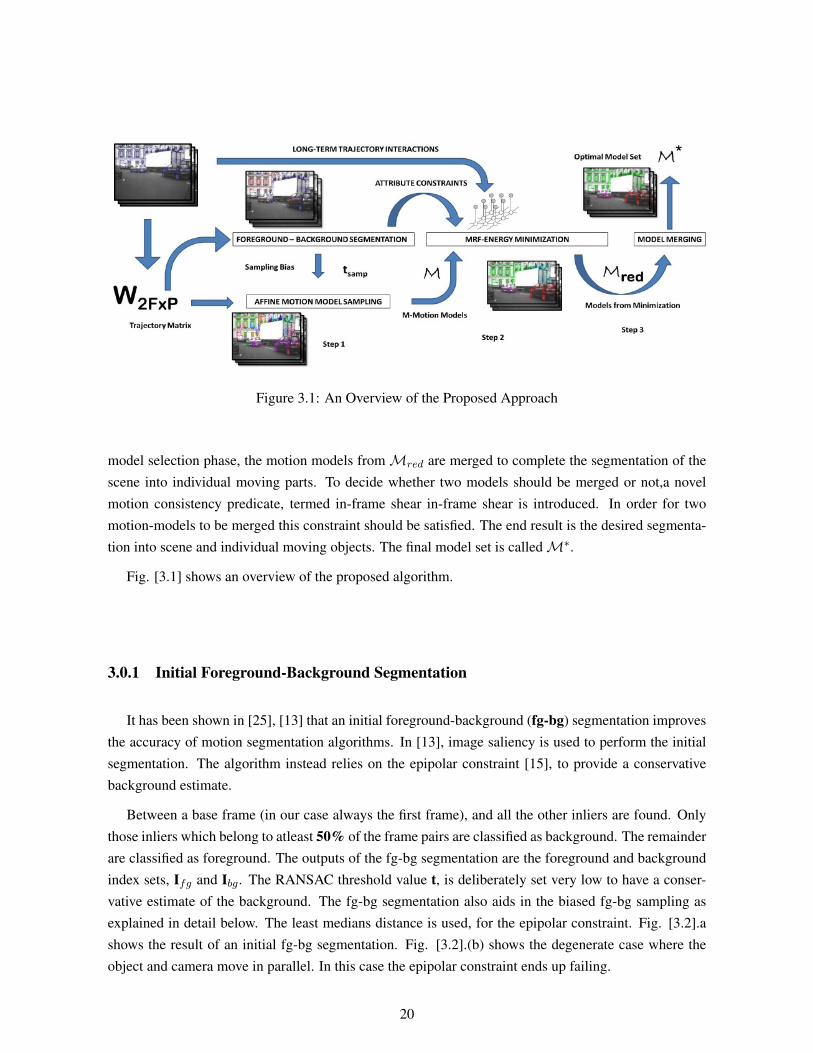
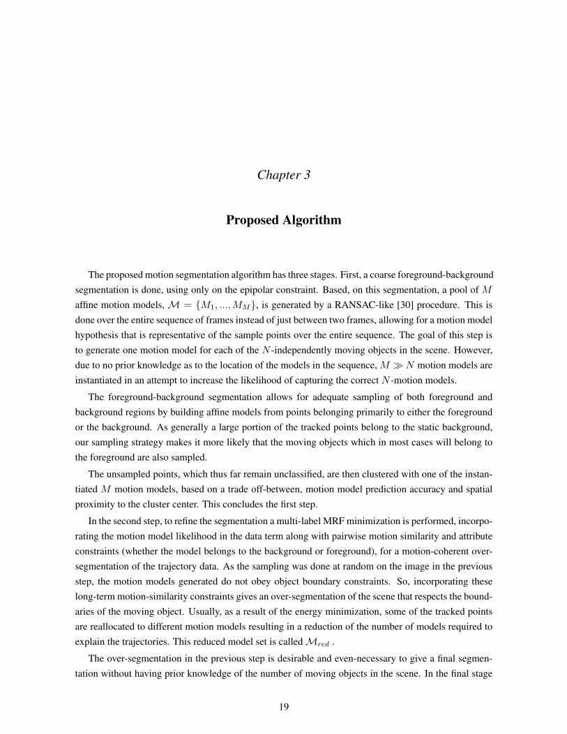
Figure 3.1: An Overview of the Proposed Approach

model selection phase, the motion models fromMred are merged to complete the segmentation of thescene into individual moving parts. To decide whether two models should be merged or not,a novelmotion consistency predicate, termed in-frame shear in-frame shear is introduced. In order for twomotion-models to be merged this constraint should be satisfied. The end result is the desired segmenta-tion into scene and individual moving objects. The final model set is calledM∗.

Fig. [3.1] shows an overview of the proposed algorithm.

3.0.1 Initial Foreground-Background Segmentation

It has been shown in [25], [13] that an initial foreground-background (fg-bg) segmentation improvesthe accuracy of motion segmentation algorithms. In [13], image saliency is used to perform the initialsegmentation. The algorithm instead relies on the epipolar constraint [15], to provide a conservativebackground estimate.

Between a base frame (in our case always the first frame), and all the other inliers are found. Onlythose inliers which belong to atleast 50% of the frame pairs are classified as background. The remainderare classified as foreground. The outputs of the fg-bg segmentation are the foreground and backgroundindex sets, Ifg and Ibg. The RANSAC threshold value t, is deliberately set very low to have a conser-vative estimate of the background. The fg-bg segmentation also aids in the biased fg-bg sampling asexplained in detail below. The least medians distance is used, for the epipolar constraint. Fig. [3.2].ashows the result of an initial fg-bg segmentation. Fig. [3.2].(b) shows the degenerate case where theobject and camera move in parallel. In this case the epipolar constraint ends up failing.

20

(a) Non-Degenerate (b) Degenerate

Figure 3.2: Figure shows a result of the initial foreground-background segmentation. The foreground(epipolar outliers) are shown in blue, and background (epipolar inliers) are shown in red. (a) In the non-degenerate case most, of the points on the moving vehicle have been categorized as not belonging to thebackground. (b) In the degenerate case, most of the points on the vehicle belong to the background.

3.0.2 Biased Affine Motion Model Sampling

From the fg-bg segmentation, the trajectory matrix can be partitioned into Wbg and Wfg , whereWfg contains only the foreground points and Wbg contains only the background points. Samplingseparately from the foreground and background makes it more likely that the samples extracted fromthe trajectory data, will accurately represent the N -independently moving objects in the scene. Thiscovers the case, where only few points are tracked on a foreground object, as frequently happens onnon-textured surfaces. It is intuitively obvious that, most of the points sampled from a small region,will belong to the same object. Keeping this idea of local coherence, in mind, disk-shaped regions, of afixed small radius, are randomly sampled as the scale of the object in question is a-priori unknown. Thisregion serves as the support set for our affine model and is defined by

W ={wi|(x1,i − cx)2 + (y1,i − cy)2 < r2

}(3.1)

Here, wi is the ith column of the trajectory matrix, x1,i and y1,i are the x and y - image coordinates ofthe ith trajectory in the first frame. (cx, cy) are the co-ordinates of the center of the disk, and r its radius.To promote a more comprehensive coverage of the scene, the number of times (cx, cy) is sampled fromthe trajectories of Wfg to the number of times from Wbg is governed by a parameter tsamp . The detailsare shown in algorithm 1.

For computation of the affine model A, three trajectories Cpts = [c1, c2, c3] are extracted from W.The affine motion model between frame 1 and f can then be computed by,

A1→f =

[cf1 cf2 cf31 1 1

][c1

1 c12 c1

3

1 1 1

]−1

(3.2)

21

Here, cfi = [xf,iyf,i] , are the x and y co-ordinates of the ith control trajectory at frame f . The inverse

of the right hand side matrix exists, except in the case where the 3 points are collinear.

Like in 3.0.1, this affine model is computed between the first and subsequent frames, and the inliersfor each affine model are computed based on a threshold tin . Only those points which are inliers foratleast 50% of the frames are considered model inliers.

The output of the affine sampling algorithm is the motion model tuple M = {Iin, Cpts, S}. Iin

contains the indices of the model inliers. Cpts are the image co-ordinates of the 3 control points in thefirst frame. S gives the attribute of the model, i.e., whether it is a foreground or background model. Itshould be noted that no use of the computed affine models is made subsequently.Insear a more robustmodel-fitting measure, described in the subsequent sub-section, is used. It was experimentally foundthat, setting the number of RANSAC iterations to as low as 10 did not affect the overall accuracy of thealgorithm, while speeding it up somewhat.

3.0.3 Initial Assignment of the Unsampled Points

To deal with points that remain unsampled after the motion model generation, it would make senseto classify the point as belonging to the affine model that explains it the best, i.e, the one with which thetrajectory has minimum residual. This is the most common strategy and is useful in situations where themodels are distinctive, and has been used in [5] and [11] successfully. However, in the case, where themodels are not distinctive and explain similar motions, this may lead to a spatially incoherent labeling.This is because, the residual value would be low and very similar for more than one models. So inaddition to a low model residual, a spatial constraint, is also imposed on the assignment.

For each unsampled trajectory wi , its residual set ri ={ri1, . . . , r

iM

}is computed from the M affine

motion model hypothesis. The elements in ri are then sorted to obtain the sorted residual set ri. For themodels that yielded the top k-elements r of this set, the Euclidean distance is calculated from the imageco-ordinates of wi and the control points of the model in the first frame. The trajectory point is allotedto the model with minimum distance.

The model residual is the orthogonal distance to the hypothesis subspace, given by,

rim = |UUTw-w| (3.3)

U is the first two left-singular vectors of matrix Wm, which contains the inlier trajectories of themth motion model. The orthogonal distance is used as error metric, instead of making direct use thecalculated affine motion model matrices (A matrices) as it is more robust to noise. However, it is stillsensitive to outliers.

Fig.[3.3] shows the contrast between a minimum residual approach versus top-k minimum residualsapproach. As can be seen clearly, spatial coherence is much better in the latter approach. The top-kresidual idea was first introduced in [19].

22

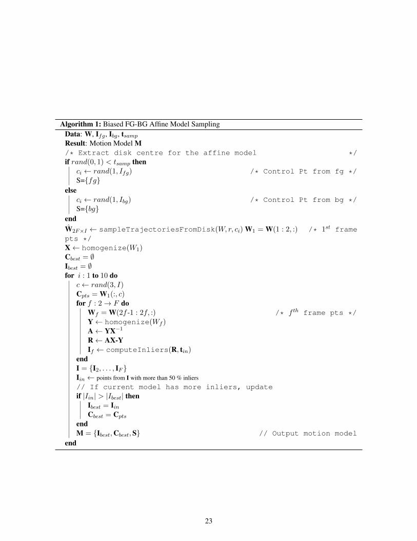
Algorithm 1: Biased FG-BG Affine Model SamplingData: W, Ifg, Ibg, tsamp

Result: Motion Model M/* Extract disk centre for the affine model */if rand(0, 1) < tsamp then

ci ← rand(1, Ifg) /* Control Pt from fg */S={fg}

elseci ← rand(1, Ibg) /* Control Pt from bg */S={bg}

endW2F×I ← sampleTrajectoriesFromDisk(W, r, ci) W1 = W(1 : 2, :) /* 1st framepts */X← homogenize(W1)Cbest = ∅Ibest = ∅for i : 1 to 10 do

c← rand(3, I)Cpts = W1(:, c)for f : 2→ F do

Wf = W(2f -1 : 2f, :) /* f th frame pts */Y← homogenize(Wf )A← YX−1

R← AX-YIf ← computeInliers(R, tin)

endI = {I2, . . . , IF }Iin ← points from I with more than 50 % inliers

// If current model has more inliers, updateif |Iin| > |Ibest| then

Ibest = IinCbest = Cpts

endM = {Ibest,Cbest,S} // Output motion model

end

23

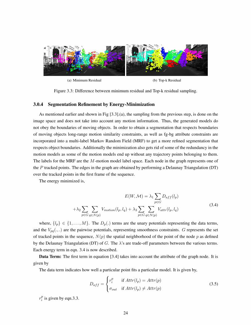
(a) Minimum Residual (b) Top-k Residual

Figure 3.3: Difference between minimum residual and Top-k residual sampling.

3.0.4 Segmentation Refinement by Energy-Minimization

As mentioned earlier and shown in Fig [3.3].(a), the sampling from the previous step, is done on theimage space and does not take into account any motion information. Thus, the generated models donot obey the boundaries of moving objects. In order to obtain a segmentation that respects boundariesof moving objects long-range motion similarity constraints, as well as fg-bg attribute constraints areincorporated into a multi-label Markov Random Field (MRF) to get a more refined segmentation thatrespects object boundaries. Additionally the minimization also gets rid of some of the redundancy in themotion models as some of the motion models end up without any trajectory points belonging to them.The labels for the MRF are the M -motion model label space. Each node in the graph represents one ofthe P tracked points. The edges in the graph are obtained by performing a Delaunay Triangulation (DT)over the tracked points in the first frame of the sequence.

The energy minimized is,

E(W,M) = λ1

∑p∈G

Daff (lp)

+λ2

∑p∈G

∑q∈N(p)

Vmotion(lp, lq) + λ3

∑p∈G

∑q∈N(p)

Vattr(lp, lq)(3.4)

where, {lp} ∈ {1, . . . ,M}. The Dp(.) terms are the unary potentials representing the data terms,and the Vpq(., .) are the pairwise potentials, representing smoothness constraints. G represents the setof tracked points in the sequence, N(p) the spatial neighborhood of the point of the node p as definedby the Delaunay Triangulation (DT) of G. The λ’s are trade-off parameters between the various terms.Each energy term in eqn. 3.4 is now described.

Data Term: The first term in equation [3.4] takes into account the attribute of the graph node. It isgiven by

The data term indicates how well a particular point fits a particular model. It is given by,

Daff =

rpi if Attr(lp) = Attr(p)

σout if Attr(lp) 6= Attr(p)(3.5)

rpi is given by eqn.3.3.

24

Cars-3 Sequence

Cars-6 Sequence

Cars-8 Sequence

Truck-1 Sequence

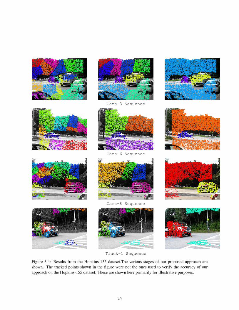
Figure 3.4: Results from the Hopkins-155 dataset.The various stages of our proposed approach areshown. The tracked points shown in the figure were not the ones used to verify the accuracy of ourapproach on the Hopkins-155 dataset. These are shown here primarily for illustrative purposes.

25

Smoothness Terms: The first smoothness term captures motion coherence. To assign similar tracksto the same clusters, the contrast-senstive Potts model given below is used.

Vmotion(lp, lq) =

0 if lp = lq

αp,q if lp 6= lq(3.6)

αp,q measures the similarity between the two tracks. It is computed using the distance between thespatial co-ordinates of track points, wp and wq for each of the frames, as well as the difference betweenthe time corresponding velocities vp and vq as below,

αp,q = exp(−(1 + ||xp − xq||2)2||vp − vq||222σ2

) (3.7)

Such motion potentials have been shown to be effective in ensuring motion coherence between tracksin [2, [29].

The second smoothness term in eqn [3.4] captures attribute coherence,

Vattr(lp, lq) =

0 if Attr(lp) = Attr(lq)

Ec if Attr(lp) 6= Attr(lq)(3.8)

Similar, attribute terms were shown to be effect in object tracking in [25]. Fig [3.4] show the resultsof the various stages of the thus far pipeline. As can be seen, we get an over-segmentation of Mred

models. For inference the Tree Re-weighted Sequential Belief Propagation Algorithm [16] is used.

3.1 Model Selection

The model-selection step is a model-merging algorithm that takes as input the set of modelsMred

and outputs the reduced setM∗ . For a particular pair of neighboring models, models are merged if, forthe model points, the model-merging predicate, Algorithm [2], is satisfied.

Initially Algorithm [3] starts of with, |Mred| distinct models. This is represented by the |Mred| ×|Mred|model-relationship matrix B, which will contain either, -1, 0 or 1 as entries. This matrix encodeswhether or not two-clusters should be merged, as follows

• if Bi,j = 0, relation between i and j still unknown.

• if Bi,j = -1, i and j belong to separate objects.

• if Bi,j = 1, i and j belong to same object.

The algorithm begins with B having 1 along the diagonals and 0 everywhere else, indicating that eachcluster is compatible with itself, and the other relations are unknown. The algorithm terminates whenall the relations are known, i.e., B has no elements as 0. For each iteration, the closest pair of clusterswhose relationship is unknown are chosen, a greedy minimum distance-based assignment is done on a

26

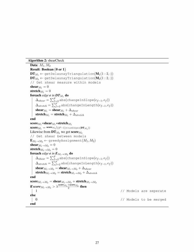
Algorithm 2: shearCheckData: M1,M2

Result: Boolean {0 or 1}DTM1 ← getDelaunayTriangulation(M1(1 : 2, :))DTM2 ← getDelaunayTriangulation(M2(1 : 2, :))// Get shear measure within modelsshearM1 = 0stretchM1 = 0foreach edge e in DTM1 do

∆shear =∑F

f=2 abs(changeInSlope(ef−1, ef ))

∆stretch =∑F

f=2 abs(changeInLength(ef−1, ef ))

shearM1 = shearM1 + ∆shear

stretchM1 = stretchM1 + ∆stretch

endscoreM1=shearM1+stretchM1

scoreM1 = scoreM1/((F−1)×numEdges(DTM1))

Likewise from DTM2 we get scoreM2

// Get shear between modelsEM1→M2 ← greedyAssignment(M1,M2)shearM1→M2 = 0stretchM1→M2 = 0foreach edge e in EM1→M2 do

∆shear =∑F

f=2 abs(changeInSlope(ef−1, ef ))

∆stretch =∑F

f=2 abs(changeInLength(ef−1, ef ))

shearM1→M2 = shearM1→M2 + ∆shear

stretchM1→M2 = stretchM1→M2 + ∆stretch

endscoreM1→M2 = shearM1→M2 + stretchM1→M2

if scoreM1→M2 > λscoreM1

+scoreM22 then

1 // Models are seperateelse

0 // Models to be mergedend

27

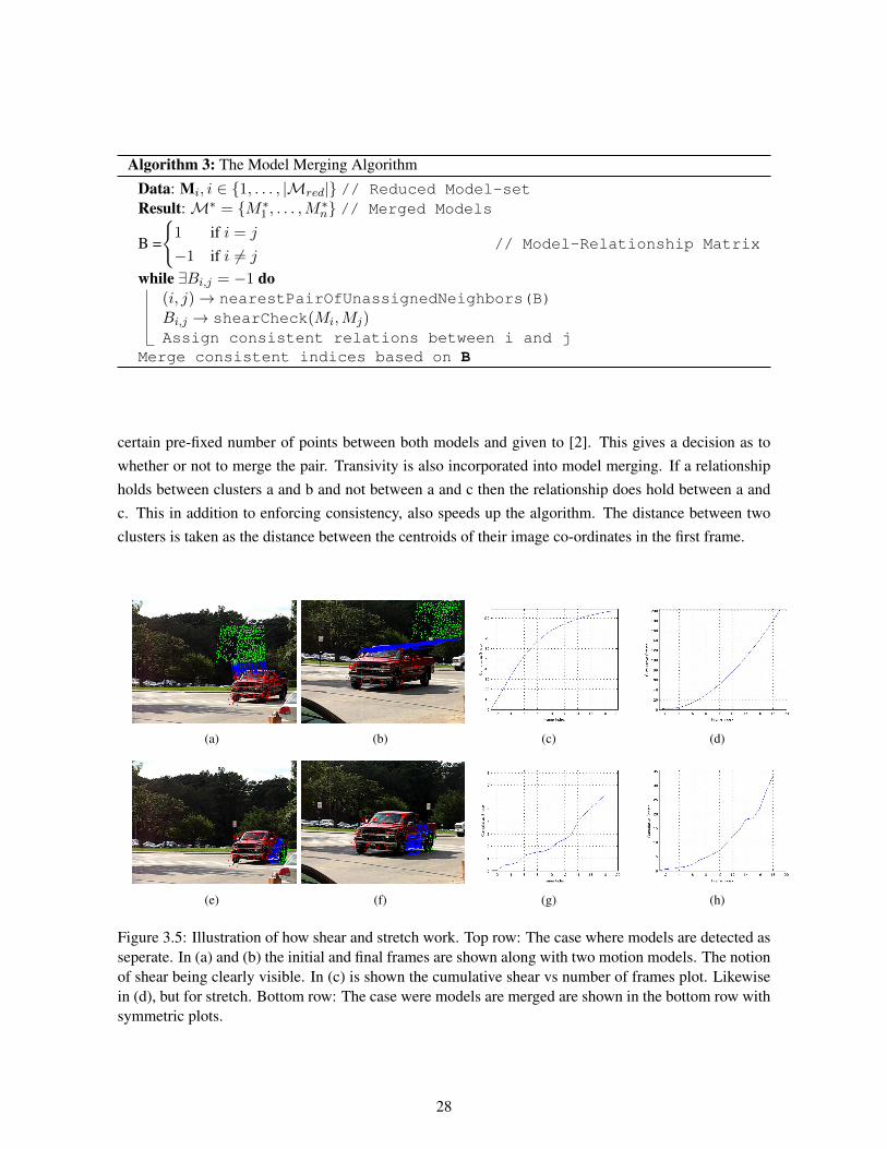
Algorithm 3: The Model Merging Algorithm

Data: Mi, i ∈ {1, . . . , |Mred|} // Reduced Model-setResult:M∗ = {M∗1 , . . . ,M∗n} // Merged Models

B =

{1 if i = j

−1 if i 6= j// Model-Relationship Matrix

while ∃Bi,j = −1 do(i, j)→ nearestPairOfUnassignedNeighbors(B)Bi,j → shearCheck(Mi,Mj)Assign consistent relations between i and j

Merge consistent indices based on B

certain pre-fixed number of points between both models and given to [2]. This gives a decision as towhether or not to merge the pair. Transivity is also incorporated into model merging. If a relationshipholds between clusters a and b and not between a and c then the relationship does hold between a andc. This in addition to enforcing consistency, also speeds up the algorithm. The distance between twoclusters is taken as the distance between the centroids of their image co-ordinates in the first frame.

(a) (b) (c) (d)

(e) (f) (g) (h)

Figure 3.5: Illustration of how shear and stretch work. Top row: The case where models are detected asseperate. In (a) and (b) the initial and final frames are shown along with two motion models. The notionof shear being clearly visible. In (c) is shown the cumulative shear vs number of frames plot. Likewisein (d), but for stretch. Bottom row: The case were models are merged are shown in the bottom row withsymmetric plots.

28

3.1.1 Model Merging Predicate

In the case of a moving camera, motion segmentation is like separating out two convolved signalsfrom each other, which is an innately hard problem. So, in an attempt to bypass the complication inducedby a moving camera, we look at relative geometric relationships in-frame that change over-time to detectmotion. For example, in Fig.[3.5].(a) the cluster in green is initially close to the vehicle in the world(cluster in red). The lines between the two initially have a predominantly downward orientation. By thelast frame, the predominant orientation has changed by around 90 degrees, as shown in Fig.[3.5].(b) andquantitatively in (c). The stretch vs frames plot is given in (d).

In general, there is a change in orientation and length-over time between the points belonging to thesame cluster, especially in scenes that have an active Focus-of-Expansion. However, this is much smallerthan the change in orientation or length, between points belonging to clusters moving with respect toeach other. Algorithm [2] is designed around this observation.

Given points from two clustersM1 andM2, we calculate the internal shear and stretch for each of themodels by calculating the average change in orientation and length, over the sequences of frames andedges of the Delaunay Triangulation of the points in the first frame. To calculate the inter-model shear,we first do a greedy minimum distance-based assignment, to assign a one-to-one mapping betweenpoints from M1 to M2. Similar to the internal shear case, the change in orientation of line-segments andlength defined by the mapping are used to calculate the inter-model shear and stretch respectively. Inorder for the models to remain seperate, the inter-model shear must be atleast a factor of λ greater thanthe average intra-model shear. For all of our experiments, we set this parameter to be 3.

One might ask whether both shearing and stretching are required, or can we just use one and reducecomputation. Generally either the shearing or the stretching dominates and not often both simultane-ously. For example, in Fig.[3.5] (c) and (d) in the initialy frames the change in angle changes drastically,while length does so much more slowly. By the end of the sequence, the change in angle had stagnated,whereas the change in length was pronounced. A possible future direction of research is doing higherlevel traffic reasoning on the basis of shear and stretch. For example, in (h) one could ue the informationthat the length between the models is increasing to infer that the object is approaching the camera. Ascan be seen by comparing (c) and (g), as well as (d) and (h), that, in the case where the models areseperate the changes in angle and length are much more pronounced.

In this chapter we elucidated the motion segmentation algorithm that forms a major portion of thisthesis. In it all three design principles mentioned in Chapter 1, were incorporated.

• Temporal Coherence - Incorporated in the MRF Minimization. (eqn. 3.7)

• Spatial Coherence - Incoprated in building motion models from small disks.

• Common Fate - Incorporated in the shear constraints.

29

Chapter 4

Results

This chapter presents a comparison of the proposed approach with several state-of-the-art algo-rithms. The comparison is done over two datasets - the Hopkins-155 and the On-Road Dataset. Acomparison of the error rate of the proposed approach with the other algorithms for the noise-lessscenario, as well as for increasing levels of Gaussian noise, is given. Additional relevant factors likecomputation time and accuracy in estimating the number of motions are also compared.

4.1 Hopkins-155 Results

The Hopkins-155 [27] dataset has been the benchmark for motion segmentation algorithms sincefirst introduced in 2007. It consists of 155 sequences: 120 and 35, for the two and three rigid mo-tions, respectively. Each sequence comes with a set of tracked points, and their ground-truth labels.The sequences are divided into three main categories - checkerboard, traffic and miscellaneous. Thecheckerboard sequences consist of upto 3 checkerboards either rotating or translating, on which pointsare tracked. Traffic sequences consist of sequences of moving vehicles taken from an unsteady hand-held camera. The miscellaneous sequences consist of articulated and non-rigid sequences.

The algorithms compared against span the more successful approaches to the motion segmentationproblem, namely the subspace clustering and the trajectory similarity based algorithm. The most basicof the subspace clustering algorithms is the RANSAC [27]. Generalized Principal Component Anal-ysis (GPCA), introduced in [77], fits a polyomial to the subspace and then classifies it. The order ofthe polynomial fit, representing it’s dimension. Spectral Curvature Clustering (SCC) [42] and SparseGrassmanian Clustering (SGC) [26] use tensor decomposition followed by subspace clustering. LinearCombination of Views (LCV) [33] samples a set of points and for them synthesizes a trajectory usingthe first and last frames of the sequence. Clustering is done on the bases of how well the actual trajec-tory corresponds to the synthesized one. Sparse Subspace Clustering (SSC) [3] models the trajectorypoints as a sparse combination of sampled trajectories. Adaptive Subspace Affinity (ASA) [45], OrderedResidual Kernel (ORK) [43] and Multiple Subspace Learning (MSL) [7] are subspace fitting algorithmscapable of handling degenerate sequences. Higher Order Spectral Clustering introduced in [48], uses

30

a combination of a motion model as well as a trajectory similarity metric like eqn. 3.7 to cluster thevarious trajectories in the scene. For the sake of brevity, the proposed approach is termed from now onas IFS (In-Frame Shear).

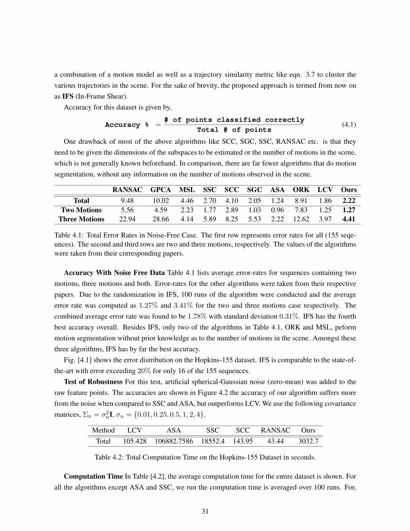
Accuracy for this dataset is given by,

Accuracy % =# of points classified correctly

Total # of points(4.1)

One drawback of most of the above algorithms like SCC, SGC, SSC, RANSAC etc. is that theyneed to be given the dimensions of the subspaces to be estimated or the number of motions in the scene,which is not generally known beforehand. In comparison, there are far fewer algorithms that do motionsegmentation, without any information on the number of motions observed in the scene.

RANSAC GPCA MSL SSC SCC SGC ASA ORK LCV OursTotal 9.48 10.02 4.46 2.70 4.10 2.05 1.24 8.91 1.86 2.22

Two Motions 5.56 4.59 2.23 1.77 2.89 1.03 0.96 7.83 1.25 1.27Three Motions 22.94 28.66 4.14 5.89 8.25 5.53 2.22 12.62 3.97 4.41

Table 4.1: Total Error Rates in Noise-Free Case. The first row represents error rates for all (155 seqe-unces). The second and third rows are two and three motions, respectively. The values of the algorithmswere taken from their corresponding papers.

Accuracy With Noise Free Data Table 4.1 lists average error-rates for sequences containing twomotions, three motions and both. Error-rates for the other algorithms were taken from their respectivepapers. Due to the randomization in IFS, 100 runs of the algorithm were conducted and the averageerror rate was computed as 1.27% and 3.41% for the two and three motions case respectively. Thecombined average error rate was found to be 1.78% with standard deviation 0.31%. IFS has the fourthbest accuracy overall. Besides IFS, only two of the algorithms in Table 4.1, ORK and MSL, peformmotion segmentation without prior knowledge as to the number of motions in the scene. Amongst thesethree algorithms, IFS has by far the best accuracy.

Fig. [4.1] shows the error distribution on the Hopkins-155 dataset. IFS is comparable to the state-of-the-art with error exceeding 20% for only 16 of the 155 sequences.

Test of Robustness For this test, artificial spherical-Gaussian noise (zero-mean) was added to theraw feature points. The accuracies are shown in Figure 4.2 the accuracy of our algorithm suffers morefrom the noise when compared to SSC and ASA, but outperforms LCV. We use the following covariancematrices, Σn = σ2

nI, σn = {0.01, 0.25, 0.5, 1, 2, 4}.

Method LCV ASA SSC SCC RANSAC OursTotal 105.428 106882.7586 18552.4 143.95 43.44 3032.7

Table 4.2: Total Computation Time on the Hopkins-155 Dataset in seconds.

Computation Time In Table [4.2], the average computation time for the entire dataset is shown. Forall the algorithms except ASA and SSC, we run the computation time is averaged over 100 runs. For,

31

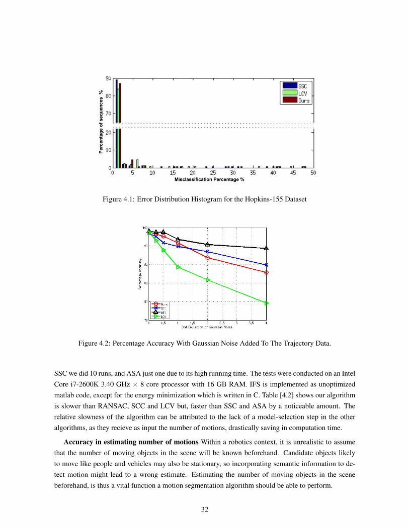
Figure 4.1: Error Distribution Histogram for the Hopkins-155 Dataset

Figure 4.2: Percentage Accuracy With Gaussian Noise Added To The Trajectory Data.

SSC we did 10 runs, and ASA just one due to its high running time. The tests were conducted on an IntelCore i7-2600K 3.40 GHz × 8 core processor with 16 GB RAM. IFS is implemented as unoptimizedmatlab code, except for the energy minimization which is written in C. Table [4.2] shows our algorithmis slower than RANSAC, SCC and LCV but, faster than SSC and ASA by a noticeable amount. Therelative slowness of the algorithm can be attributed to the lack of a model-selection step in the otheralgorithms, as they recieve as input the number of motions, drastically saving in computation time.

Accuracy in estimating number of motions Within a robotics context, it is unrealistic to assumethat the number of moving objects in the scene will be known beforehand. Candidate objects likelyto move like people and vehicles may also be stationary, so incorporating semantic information to de-tect motion might lead to a wrong estimate. Estimating the number of moving objects in the scenebeforehand, is thus a vital function a motion segmentation algorithm should be able to perform.

32

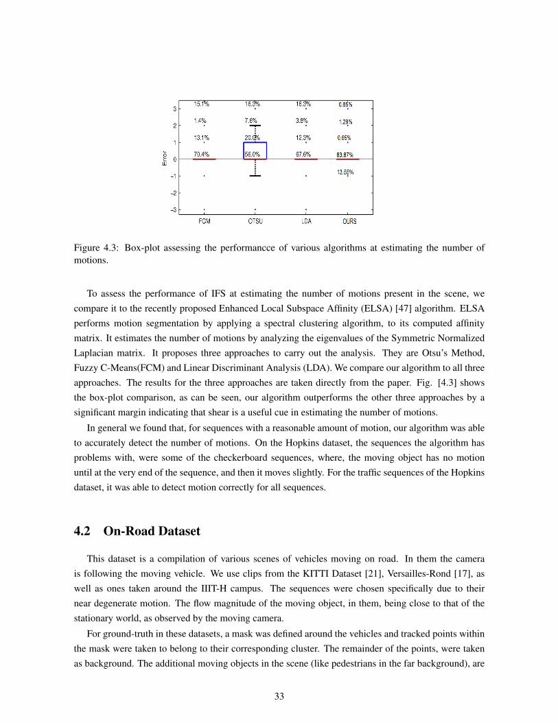
Figure 4.3: Box-plot assessing the performancce of various algorithms at estimating the number ofmotions.

To assess the performance of IFS at estimating the number of motions present in the scene, wecompare it to the recently proposed Enhanced Local Subspace Affinity (ELSA) [47] algorithm. ELSAperforms motion segmentation by applying a spectral clustering algorithm, to its computed affinitymatrix. It estimates the number of motions by analyzing the eigenvalues of the Symmetric NormalizedLaplacian matrix. It proposes three approaches to carry out the analysis. They are Otsu’s Method,Fuzzy C-Means(FCM) and Linear Discriminant Analysis (LDA). We compare our algorithm to all threeapproaches. The results for the three approaches are taken directly from the paper. Fig. [4.3] showsthe box-plot comparison, as can be seen, our algorithm outperforms the other three approaches by asignificant margin indicating that shear is a useful cue in estimating the number of motions.

In general we found that, for sequences with a reasonable amount of motion, our algorithm was ableto accurately detect the number of motions. On the Hopkins dataset, the sequences the algorithm hasproblems with, were some of the checkerboard sequences, where, the moving object has no motionuntil at the very end of the sequence, and then it moves slightly. For the traffic sequences of the Hopkinsdataset, it was able to detect motion correctly for all sequences.

4.2 On-Road Dataset

This dataset is a compilation of various scenes of vehicles moving on road. In them the camerais following the moving vehicle. We use clips from the KITTI Dataset [21], Versailles-Rond [17], aswell as ones taken around the IIIT-H campus. The sequences were chosen specifically due to theirnear degenerate motion. The flow magnitude of the moving object, in them, being close to that of thestationary world, as observed by the moving camera.

For ground-truth in these datasets, a mask was defined around the vehicles and tracked points withinthe mask were taken to belong to their corresponding cluster. The remainder of the points, were takenas background. The additional moving objects in the scene (like pedestrians in the far background), are

33

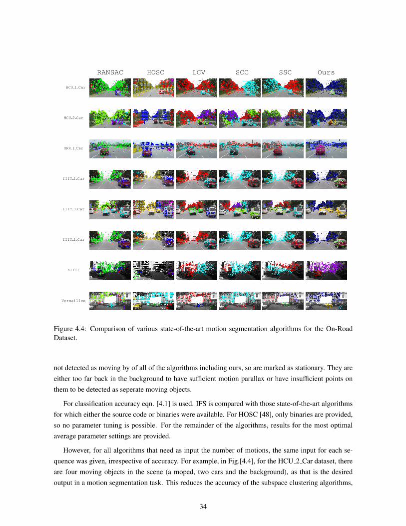
RANSAC HOSC LCV SCC SSC Ours

HCU 1 Car

HCU 2 Car

ORR 1 Car

IIIT 1 Car

IIIT 3 Car

IIIT 1 Car

KITTI

Versailles

Figure 4.4: Comparison of various state-of-the-art motion segmentation algorithms for the On-RoadDataset.

not detected as moving by of all of the algorithms including ours, so are marked as stationary. They areeither too far back in the background to have sufficient motion parallax or have insufficient points onthem to be detected as seperate moving objects.

For classification accuracy eqn. [4.1] is used. IFS is compared with those state-of-the-art algorithmsfor which either the source code or binaries were available. For HOSC [48], only binaries are provided,so no parameter tuning is possible. For the remainder of the algorithms, results for the most optimalaverage parameter settings are provided.

However, for all algorithms that need as input the number of motions, the same input for each se-quence was given, irrespective of accuracy. For example, in Fig.[4.4], for the HCU 2 Car dataset, thereare four moving objects in the scene (a moped, two cars and the background), as that is the desiredoutput in a motion segmentation task. This reduces the accuracy of the subspace clustering algorithms,

34

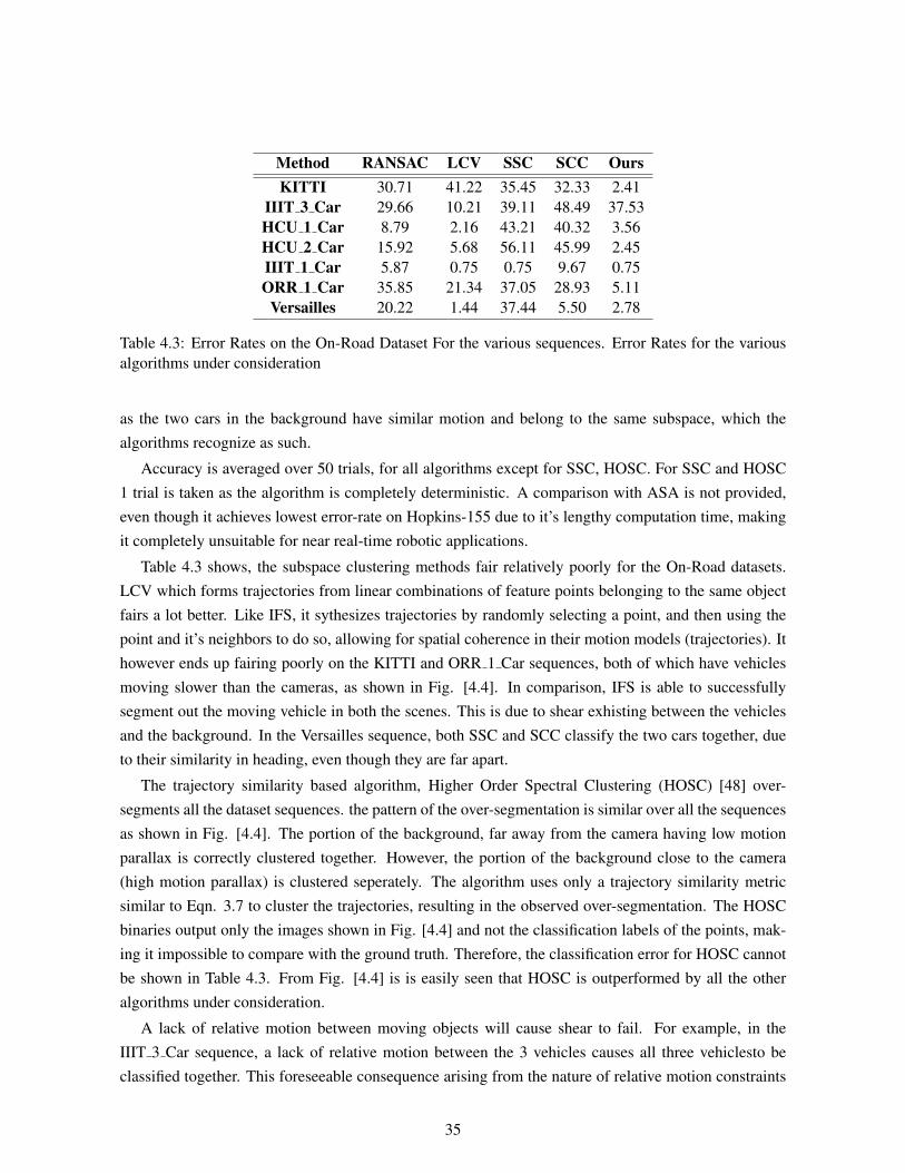
Method RANSAC LCV SSC SCC OursKITTI 30.71 41.22 35.45 32.33 2.41

IIIT 3 Car 29.66 10.21 39.11 48.49 37.53HCU 1 Car 8.79 2.16 43.21 40.32 3.56HCU 2 Car 15.92 5.68 56.11 45.99 2.45IIIT 1 Car 5.87 0.75 0.75 9.67 0.75ORR 1 Car 35.85 21.34 37.05 28.93 5.11

Versailles 20.22 1.44 37.44 5.50 2.78

Table 4.3: Error Rates on the On-Road Dataset For the various sequences. Error Rates for the variousalgorithms under consideration

as the two cars in the background have similar motion and belong to the same subspace, which thealgorithms recognize as such.

Accuracy is averaged over 50 trials, for all algorithms except for SSC, HOSC. For SSC and HOSC1 trial is taken as the algorithm is completely deterministic. A comparison with ASA is not provided,even though it achieves lowest error-rate on Hopkins-155 due to it’s lengthy computation time, makingit completely unsuitable for near real-time robotic applications.

Table 4.3 shows, the subspace clustering methods fair relatively poorly for the On-Road datasets.LCV which forms trajectories from linear combinations of feature points belonging to the same objectfairs a lot better. Like IFS, it sythesizes trajectories by randomly selecting a point, and then using thepoint and it’s neighbors to do so, allowing for spatial coherence in their motion models (trajectories). Ithowever ends up fairing poorly on the KITTI and ORR 1 Car sequences, both of which have vehiclesmoving slower than the cameras, as shown in Fig. [4.4]. In comparison, IFS is able to successfullysegment out the moving vehicle in both the scenes. This is due to shear exhisting between the vehiclesand the background. In the Versailles sequence, both SSC and SCC classify the two cars together, dueto their similarity in heading, even though they are far apart.

The trajectory similarity based algorithm, Higher Order Spectral Clustering (HOSC) [48] over-segments all the dataset sequences. the pattern of the over-segmentation is similar over all the sequencesas shown in Fig. [4.4]. The portion of the background, far away from the camera having low motionparallax is correctly clustered together. However, the portion of the background close to the camera(high motion parallax) is clustered seperately. The algorithm uses only a trajectory similarity metricsimilar to Eqn. 3.7 to cluster the trajectories, resulting in the observed over-segmentation. The HOSCbinaries output only the images shown in Fig. [4.4] and not the classification labels of the points, mak-ing it impossible to compare with the ground truth. Therefore, the classification error for HOSC cannotbe shown in Table 4.3. From Fig. [4.4] is is easily seen that HOSC is outperformed by all the otheralgorithms under consideration.

A lack of relative motion between moving objects will cause shear to fail. For example, in theIIIT 3 Car sequence, a lack of relative motion between the 3 vehicles causes all three vehiclesto beclassified together. This foreseeable consequence arising from the nature of relative motion constraints

35

probably indicates that using only motion cues, leaves the motion segmentation problem ill-posed. Ifin addition, an object detector, were used, to recognize all possible moving objects like pedestrians andvehicles, and shear constraints were checked between them and the background (area not containing po-tentially moving objects), the algorithm would perform more optimally. One can see that the stationaryvehicles and pedestrains, detected by an object detector, in the scene would be merged with the back-ground and the moving objects would belong to their own seperate clusters irrespective of the relativemotion between the objects.

Overall, table 4.3 and Fig. [4.4] shows that incorporating only trajectory similarity cues is insufficientfor motion segmentation in the case of a moving camera, as shown in the HOSC case. Likewise, usingonly subspace information frequently results in an erroneous estimation of the moving objects, due totheir similarity in motion with the background. The superior performance of both LCV and IFS, canbe attributed to a similar initial step. In both cases, motion models are calculated from nearby points,incorporating spatial coherence into the algorithms. Thus spatial coherence is a valuable attribute amotion segmentation algorithm should possess.

36

Chapter 5

Conclusions

In this thesis a motion segmentation algorithm (IFS), for trajectory data, capable of handling bothdegenerate and non-degenerate algorithms, was introduced. It takes images in batch, and on the basis ofjudicious use of geometric and gestalt motion cues, performs the segmentation.

The algorithm initially samples a large number of affine motion models. Information from thesemotion models along with long-term motion cues are integrated into an MRF-energy function. Thenumber of motion models obtained after the energy minimization is typically larger than the number ofmoving objects in the scene. This over-segmentation, is crucial and necessary in dealing with degeneratecases, where camera and object motion are nearly the same. The third, and final step involves mergingthe models from the reduced motion model set of the previous step based on a novel motion similarityconstraint, explained in Section 3.1.1. The similarity constraint, termed in-frame shear, measures therelative change in geometry between two motion models as observable from a monocular sequence ofimages.

Through experiments it was showed that IFS is comprable with the state-of-the-art in terms of clas-sification accuracy. It was faster than all of the other algorithms with comparable accuracy except LCV.One big advantage the algorithm has over other methods is it does so without knowing the number ofmotions beforehand. For the real-world datasets it was tested on it outperformed the other algorithmsby a substantial margin.

A possible future direction of research would be to combine the proposed framework with objectdetection algorithms like [9]. This would allow a precise sampling of regions of interest in the image,reducing the number of motion models M in the scene significantly, speeding up the overall algorithm.For example, detecting possible moving objects like pedestrians and vehicles in a road like scenario andcomparing shear constraints only between background and moving object models would allow for themotion segmentation algorithms to detect all three vehicles in the IIIT 3 Car sequence.

37

Related Publications

1. Siddharth Tourani and K Madhava Krishna “Using In-Frame Shear Constraints for MonocularMotion Segmentation”. Indian Conference on Vision, Graphics and Image Processing,(Oral),2014.

2. Siddharth Tourani and K Madhava Krishna, “Monocular Motion Segmentation of Rigid BodiesUsing In-Frame Shear Constraints”, Journal of Intelligent Robotics and Systems., (Submitted)

38

Bibliography

[1] Namdev, R. K., Kundu, A., Krishna, K. M., Jawahar, C. V., (2012, May). Motion segmentationof multiple objects from a freely moving monocular camera. In Robotics and Automation (ICRA),2012 IEEE International Conference on (pp. 4092-4099). IEEE.

[2] Lezama, J., Alahari, K., Sivic, J., Laptev, I. (2011, June). Track to the future: Spatio-temporal videosegmentation with long-range motion cues. In Computer Vision and Pattern Recognition (CVPR),2011 IEEE Conference on. IEEE.

[3] Elhamifar, E., Vidal, R. (2009, June). Sparse subspace clustering. In Computer Vision and PatternRecognition, 2009. CVPR 2009. IEEE Conference on (pp. 2790-2797). IEEE.

[4] Sugaya, Y., Kanatani, K. (2004). Geometric structure of degeneracy for multi-body motion segmen-tation. In Statistical Methods in Video Processing (pp. 13-25). Springer Berlin Heidelberg.

[5] Flores-Mangas, F., Jepson, A. D. (2013, June). Fast Rigid Motion Segmentation via Incrementally-Complex Local Models. In Computer Vision and Pattern Recognition (CVPR), 2013 IEEE Confer-ence on (pp. 2259-2266). IEEE.

[6] Yan, J., Pollefeys, M. (2006). A general framework for motion segmentation: Independent, ar-ticulated, rigid, non-rigid, degenerate and non-degenerate. In Computer Vision ECCV 2006 (pp.94-106). Springer Berlin Heidelberg.

[7] K. Kanatani. Motion segmentation by subspace separation and model selection. In IEEE Interna-tional Conference on Computer Vision, volume 2, pages 586591, 2001.

[8] Rao, S. R., Tron, R., Vidal, R., Ma, Y. (2008, June). Motion segmentation via robust subspaceseparation in the presence of outlying, incomplete, or corrupted trajectories. In Computer Visionand Pattern Recognition, 2008. CVPR 2008. IEEE Conference on (pp. 1-8). IEEE.

[9] Felzenszwalb, P. F., Girshick, R. B., McAllester, D., Ramanan, D. (2010). Object detection withdiscriminatively trained part-based models. Pattern Analysis and Machine Intelligence, IEEE Trans-actions on, 32(9), 1627-1645.

39

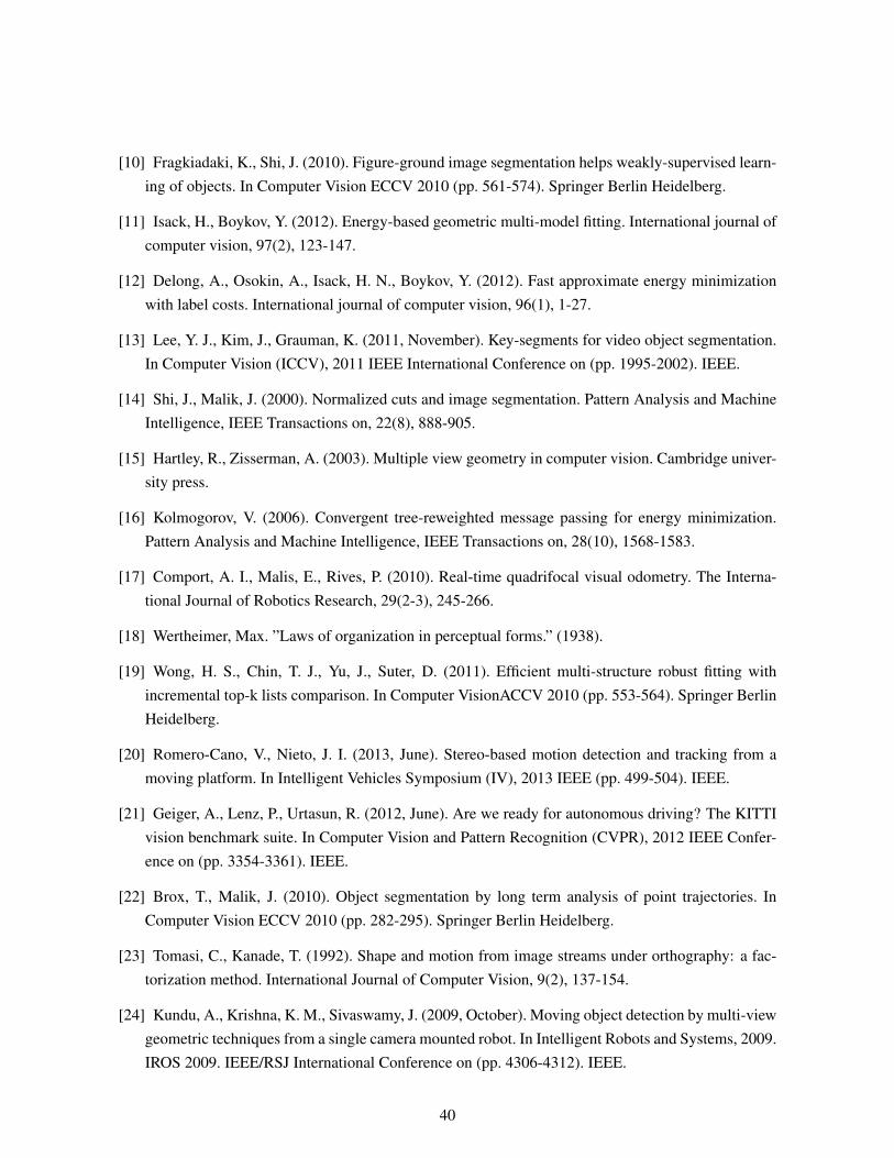
[10] Fragkiadaki, K., Shi, J. (2010). Figure-ground image segmentation helps weakly-supervised learn-ing of objects. In Computer Vision ECCV 2010 (pp. 561-574). Springer Berlin Heidelberg.

[11] Isack, H., Boykov, Y. (2012). Energy-based geometric multi-model fitting. International journal ofcomputer vision, 97(2), 123-147.

[12] Delong, A., Osokin, A., Isack, H. N., Boykov, Y. (2012). Fast approximate energy minimizationwith label costs. International journal of computer vision, 96(1), 1-27.

[13] Lee, Y. J., Kim, J., Grauman, K. (2011, November). Key-segments for video object segmentation.In Computer Vision (ICCV), 2011 IEEE International Conference on (pp. 1995-2002). IEEE.

[14] Shi, J., Malik, J. (2000). Normalized cuts and image segmentation. Pattern Analysis and MachineIntelligence, IEEE Transactions on, 22(8), 888-905.

[15] Hartley, R., Zisserman, A. (2003). Multiple view geometry in computer vision. Cambridge univer-sity press.

[16] Kolmogorov, V. (2006). Convergent tree-reweighted message passing for energy minimization.Pattern Analysis and Machine Intelligence, IEEE Transactions on, 28(10), 1568-1583.

[17] Comport, A. I., Malis, E., Rives, P. (2010). Real-time quadrifocal visual odometry. The Interna-tional Journal of Robotics Research, 29(2-3), 245-266.

[18] Wertheimer, Max. ”Laws of organization in perceptual forms.” (1938).

[19] Wong, H. S., Chin, T. J., Yu, J., Suter, D. (2011). Efficient multi-structure robust fitting withincremental top-k lists comparison. In Computer VisionACCV 2010 (pp. 553-564). Springer BerlinHeidelberg.

[20] Romero-Cano, V., Nieto, J. I. (2013, June). Stereo-based motion detection and tracking from amoving platform. In Intelligent Vehicles Symposium (IV), 2013 IEEE (pp. 499-504). IEEE.

[21] Geiger, A., Lenz, P., Urtasun, R. (2012, June). Are we ready for autonomous driving? The KITTIvision benchmark suite. In Computer Vision and Pattern Recognition (CVPR), 2012 IEEE Confer-ence on (pp. 3354-3361). IEEE.

[22] Brox, T., Malik, J. (2010). Object segmentation by long term analysis of point trajectories. InComputer Vision ECCV 2010 (pp. 282-295). Springer Berlin Heidelberg.

[23] Tomasi, C., Kanade, T. (1992). Shape and motion from image streams under orthography: a fac-torization method. International Journal of Computer Vision, 9(2), 137-154.

[24] Kundu, A., Krishna, K. M., Sivaswamy, J. (2009, October). Moving object detection by multi-viewgeometric techniques from a single camera mounted robot. In Intelligent Robots and Systems, 2009.IROS 2009. IEEE/RSJ International Conference on (pp. 4306-4312). IEEE.

40

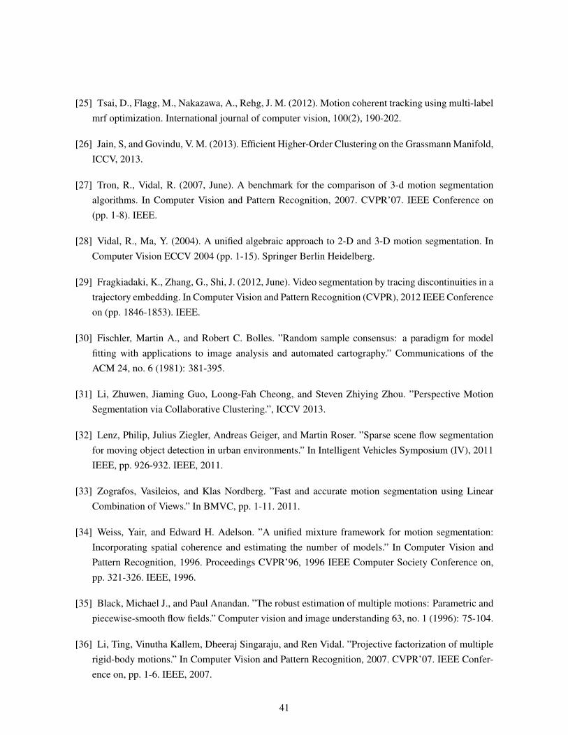
[25] Tsai, D., Flagg, M., Nakazawa, A., Rehg, J. M. (2012). Motion coherent tracking using multi-labelmrf optimization. International journal of computer vision, 100(2), 190-202.

[26] Jain, S, and Govindu, V. M. (2013). Efficient Higher-Order Clustering on the Grassmann Manifold,ICCV, 2013.

[27] Tron, R., Vidal, R. (2007, June). A benchmark for the comparison of 3-d motion segmentationalgorithms. In Computer Vision and Pattern Recognition, 2007. CVPR’07. IEEE Conference on(pp. 1-8). IEEE.

[28] Vidal, R., Ma, Y. (2004). A unified algebraic approach to 2-D and 3-D motion segmentation. InComputer Vision ECCV 2004 (pp. 1-15). Springer Berlin Heidelberg.

[29] Fragkiadaki, K., Zhang, G., Shi, J. (2012, June). Video segmentation by tracing discontinuities in atrajectory embedding. In Computer Vision and Pattern Recognition (CVPR), 2012 IEEE Conferenceon (pp. 1846-1853). IEEE.

[30] Fischler, Martin A., and Robert C. Bolles. ”Random sample consensus: a paradigm for modelfitting with applications to image analysis and automated cartography.” Communications of theACM 24, no. 6 (1981): 381-395.

[31] Li, Zhuwen, Jiaming Guo, Loong-Fah Cheong, and Steven Zhiying Zhou. ”Perspective MotionSegmentation via Collaborative Clustering.”, ICCV 2013.

[32] Lenz, Philip, Julius Ziegler, Andreas Geiger, and Martin Roser. ”Sparse scene flow segmentationfor moving object detection in urban environments.” In Intelligent Vehicles Symposium (IV), 2011IEEE, pp. 926-932. IEEE, 2011.

[33] Zografos, Vasileios, and Klas Nordberg. ”Fast and accurate motion segmentation using LinearCombination of Views.” In BMVC, pp. 1-11. 2011.

[34] Weiss, Yair, and Edward H. Adelson. ”A unified mixture framework for motion segmentation:Incorporating spatial coherence and estimating the number of models.” In Computer Vision andPattern Recognition, 1996. Proceedings CVPR’96, 1996 IEEE Computer Society Conference on,pp. 321-326. IEEE, 1996.

[35] Black, Michael J., and Paul Anandan. ”The robust estimation of multiple motions: Parametric andpiecewise-smooth flow fields.” Computer vision and image understanding 63, no. 1 (1996): 75-104.

[36] Li, Ting, Vinutha Kallem, Dheeraj Singaraju, and Ren Vidal. ”Projective factorization of multiplerigid-body motions.” In Computer Vision and Pattern Recognition, 2007. CVPR’07. IEEE Confer-ence on, pp. 1-6. IEEE, 2007.

41

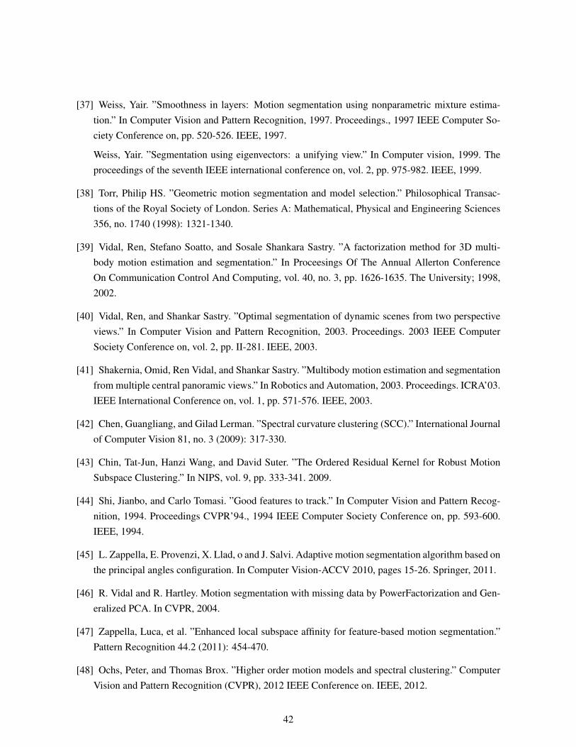
[37] Weiss, Yair. ”Smoothness in layers: Motion segmentation using nonparametric mixture estima-tion.” In Computer Vision and Pattern Recognition, 1997. Proceedings., 1997 IEEE Computer So-ciety Conference on, pp. 520-526. IEEE, 1997.

Weiss, Yair. ”Segmentation using eigenvectors: a unifying view.” In Computer vision, 1999. Theproceedings of the seventh IEEE international conference on, vol. 2, pp. 975-982. IEEE, 1999.

[38] Torr, Philip HS. ”Geometric motion segmentation and model selection.” Philosophical Transac-tions of the Royal Society of London. Series A: Mathematical, Physical and Engineering Sciences356, no. 1740 (1998): 1321-1340.

[39] Vidal, Ren, Stefano Soatto, and Sosale Shankara Sastry. ”A factorization method for 3D multi-body motion estimation and segmentation.” In Proceesings Of The Annual Allerton ConferenceOn Communication Control And Computing, vol. 40, no. 3, pp. 1626-1635. The University; 1998,2002.

[40] Vidal, Ren, and Shankar Sastry. ”Optimal segmentation of dynamic scenes from two perspectiveviews.” In Computer Vision and Pattern Recognition, 2003. Proceedings. 2003 IEEE ComputerSociety Conference on, vol. 2, pp. II-281. IEEE, 2003.

[41] Shakernia, Omid, Ren Vidal, and Shankar Sastry. ”Multibody motion estimation and segmentationfrom multiple central panoramic views.” In Robotics and Automation, 2003. Proceedings. ICRA’03.IEEE International Conference on, vol. 1, pp. 571-576. IEEE, 2003.

[42] Chen, Guangliang, and Gilad Lerman. ”Spectral curvature clustering (SCC).” International Journalof Computer Vision 81, no. 3 (2009): 317-330.

[43] Chin, Tat-Jun, Hanzi Wang, and David Suter. ”The Ordered Residual Kernel for Robust MotionSubspace Clustering.” In NIPS, vol. 9, pp. 333-341. 2009.

[44] Shi, Jianbo, and Carlo Tomasi. ”Good features to track.” In Computer Vision and Pattern Recog-nition, 1994. Proceedings CVPR’94., 1994 IEEE Computer Society Conference on, pp. 593-600.IEEE, 1994.

[45] L. Zappella, E. Provenzi, X. Llad, o and J. Salvi. Adaptive motion segmentation algorithm based onthe principal angles configuration. In Computer Vision-ACCV 2010, pages 15-26. Springer, 2011.

[46] R. Vidal and R. Hartley. Motion segmentation with missing data by PowerFactorization and Gen-eralized PCA. In CVPR, 2004.

[47] Zappella, Luca, et al. ”Enhanced local subspace affinity for feature-based motion segmentation.”Pattern Recognition 44.2 (2011): 454-470.

[48] Ochs, Peter, and Thomas Brox. ”Higher order motion models and spectral clustering.” ComputerVision and Pattern Recognition (CVPR), 2012 IEEE Conference on. IEEE, 2012.

42

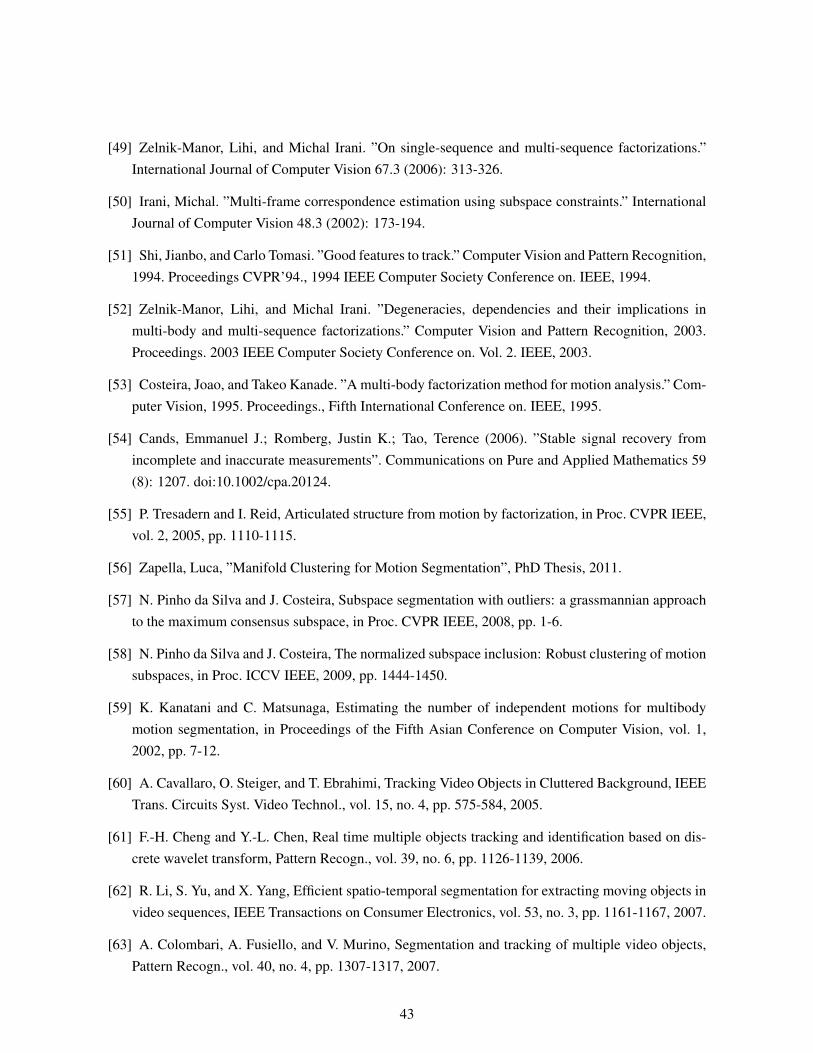
[49] Zelnik-Manor, Lihi, and Michal Irani. ”On single-sequence and multi-sequence factorizations.”International Journal of Computer Vision 67.3 (2006): 313-326.

[50] Irani, Michal. ”Multi-frame correspondence estimation using subspace constraints.” InternationalJournal of Computer Vision 48.3 (2002): 173-194.

[51] Shi, Jianbo, and Carlo Tomasi. ”Good features to track.” Computer Vision and Pattern Recognition,1994. Proceedings CVPR’94., 1994 IEEE Computer Society Conference on. IEEE, 1994.

[52] Zelnik-Manor, Lihi, and Michal Irani. ”Degeneracies, dependencies and their implications inmulti-body and multi-sequence factorizations.” Computer Vision and Pattern Recognition, 2003.Proceedings. 2003 IEEE Computer Society Conference on. Vol. 2. IEEE, 2003.

[53] Costeira, Joao, and Takeo Kanade. ”A multi-body factorization method for motion analysis.” Com-puter Vision, 1995. Proceedings., Fifth International Conference on. IEEE, 1995.

[54] Cands, Emmanuel J.; Romberg, Justin K.; Tao, Terence (2006). ”Stable signal recovery fromincomplete and inaccurate measurements”. Communications on Pure and Applied Mathematics 59(8): 1207. doi:10.1002/cpa.20124.

[55] P. Tresadern and I. Reid, Articulated structure from motion by factorization, in Proc. CVPR IEEE,vol. 2, 2005, pp. 1110-1115.

[56] Zapella, Luca, ”Manifold Clustering for Motion Segmentation”, PhD Thesis, 2011.

[57] N. Pinho da Silva and J. Costeira, Subspace segmentation with outliers: a grassmannian approachto the maximum consensus subspace, in Proc. CVPR IEEE, 2008, pp. 1-6.

[58] N. Pinho da Silva and J. Costeira, The normalized subspace inclusion: Robust clustering of motionsubspaces, in Proc. ICCV IEEE, 2009, pp. 1444-1450.

[59] K. Kanatani and C. Matsunaga, Estimating the number of independent motions for multibodymotion segmentation, in Proceedings of the Fifth Asian Conference on Computer Vision, vol. 1,2002, pp. 7-12.

[60] A. Cavallaro, O. Steiger, and T. Ebrahimi, Tracking Video Objects in Cluttered Background, IEEETrans. Circuits Syst. Video Technol., vol. 15, no. 4, pp. 575-584, 2005.

[61] F.-H. Cheng and Y.-L. Chen, Real time multiple objects tracking and identification based on dis-crete wavelet transform, Pattern Recogn., vol. 39, no. 6, pp. 1126-1139, 2006.

[62] R. Li, S. Yu, and X. Yang, Efficient spatio-temporal segmentation for extracting moving objects invideo sequences, IEEE Transactions on Consumer Electronics, vol. 53, no. 3, pp. 1161-1167, 2007.

[63] A. Colombari, A. Fusiello, and V. Murino, Segmentation and tracking of multiple video objects,Pattern Recogn., vol. 40, no. 4, pp. 1307-1317, 2007.

43

[64] B. Horn and B. Schunck, Determining optical flow, Artificial Intelligence, vol. 17, pp. 185-203,1981.

[65] E. Trucco, T. Tommasini, and V. Roberto, Near-recursive optical flow from weighted image differ-ences, IEEE Trans. Syst., Man, Cybern., vol. 35, no. 1, pp. 124-129, 2005.

[66] J. Zhang, F. Shi, J. Wang, and Y. Liu, 3d motion segmentation from straight-line optical flow, inMultimedia Content Analysis and Mining, 2007, pp. 85-94.

[67] L. Xu, J. Chen, and J. Jia, A segmentation based variational model for accurate optical flow esti-mation, in Lect. Notes Comput. Sc. (ECCV), 2008, pp. 671-684.

[68] Y. Cheng, Mean shift, mode seeking, and clustering, IEEE Trans. Pattern Analysis Machine Intell.,vol. 17, no. 8, pp. 790-799, 1995.

[69] J. Wang and E. Adelson, Layered representation for motion analysis, in Proc. CVPR IEEE, 1993,pp. 361-366.

[70] M. P. Kumar, P. H. Torr, and A. Zisserman, Learning layered motion segmentations of video, Int.J. Comput. Vision, vol. 76, no. 3, pp. 301-319, 2008.

[71] A. Gruber and Y. Weiss, Multibody factorization with uncertainty and missing data using the emalgorithm, in Proc. CVPR IEEE, vol. 1, 2004, pp. 707-714.

[72] A. Gruber and Y. Weiss, Incorporating non-motion cues into 3d motion segmentation, in Lect.Notes Comput. Sc. (ECCV), 2006, pp. 84-97.

[73] S. R. Rao, R. Tron, R. Vidal, and Y. Ma, Motion segmentation via robust subspace separation inthe presence of outlying, incomplete, or corrupted trajectories, in Proc. CVPR IEEE, 2008, pp. 1-8.

[74] Y. Ma, H. Derksen, W. Hong, and J. Wright, Segmentation of multivariate mixed data via lossydata coding and compression, IEEE Trans. Pattern Analysis Machine Intell., vol. 29, no. 9, pp.1546-1562, 2007.

[75] R. Vidal and R. Hartley, Motion segmentation with missing data using powerfactorization andgpca, in Proc. CVPR IEEE, vol. 2, 2004, pp. 310-316.

[76] R. Hartley and F. Schaffalizky, Powerfactorization: 3d reconstruction with missing or uncertaindata, in Australia-Japan Advanced Workshop on Computer Vision, 2003.

[77] R. Vidal, Y. Ma, and S. Sastry, Generalized principal component analysis (gpca), IEEE Trans.Pattern Analysis Machine Intell., vol. 27, pp. 1945-1959, 2005.

[78] K. Nordberg and V. Zografos, Multibody motion segmentation using the geometry of 6 points in2d images, in Proc. Int. C. Patt. Recog., 2010, pp. 1783-1787.

44