Intro to DataFrames and Spark SQL July, 2015

Welcome message from author
This document is posted to help you gain knowledge. Please leave a comment to let me know what you think about it! Share it to your friends and learn new things together.
Transcript
Intro to DataFrames and Spark SQL
July, 2015
Spark SQL
2
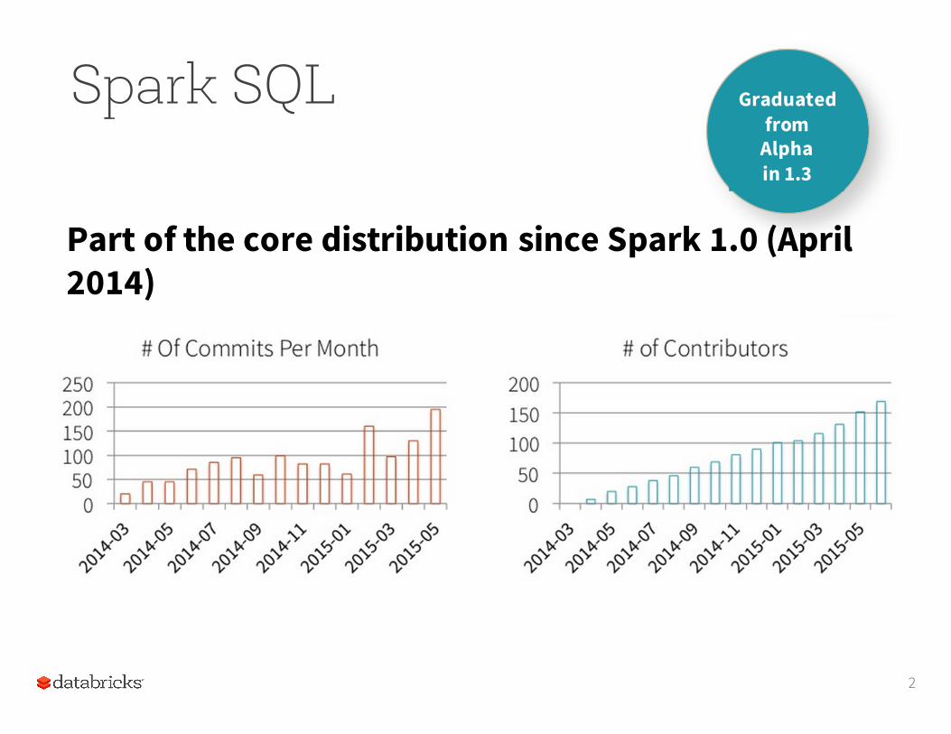
Part of the core distribution since Spark 1.0 (April 2014)
Graduatedfrom
Alphain 1.3
Spark SQL
3
Improved multi-version support in 1.4
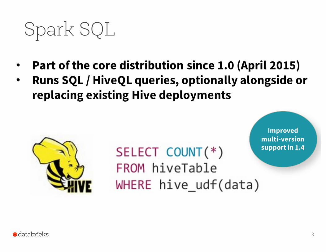
• Part of the core distribution since 1.0 (April 2015)• Runs SQL / HiveQL queries, optionally alongside or
replacing existing Hive deployments
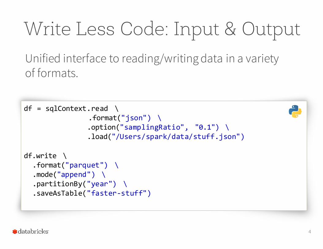
Write Less Code: Input & OutputUnified interface to reading/writing data in a variety of formats.
4
df = sqlContext.read \.format("json") \.option("samplingRatio", "0.1") \.load("/Users/spark/data/stuff.json")
df.write \.format("parquet") \.mode("append") \.partitionBy("year") \.saveAsTable("faster-‐stuff")
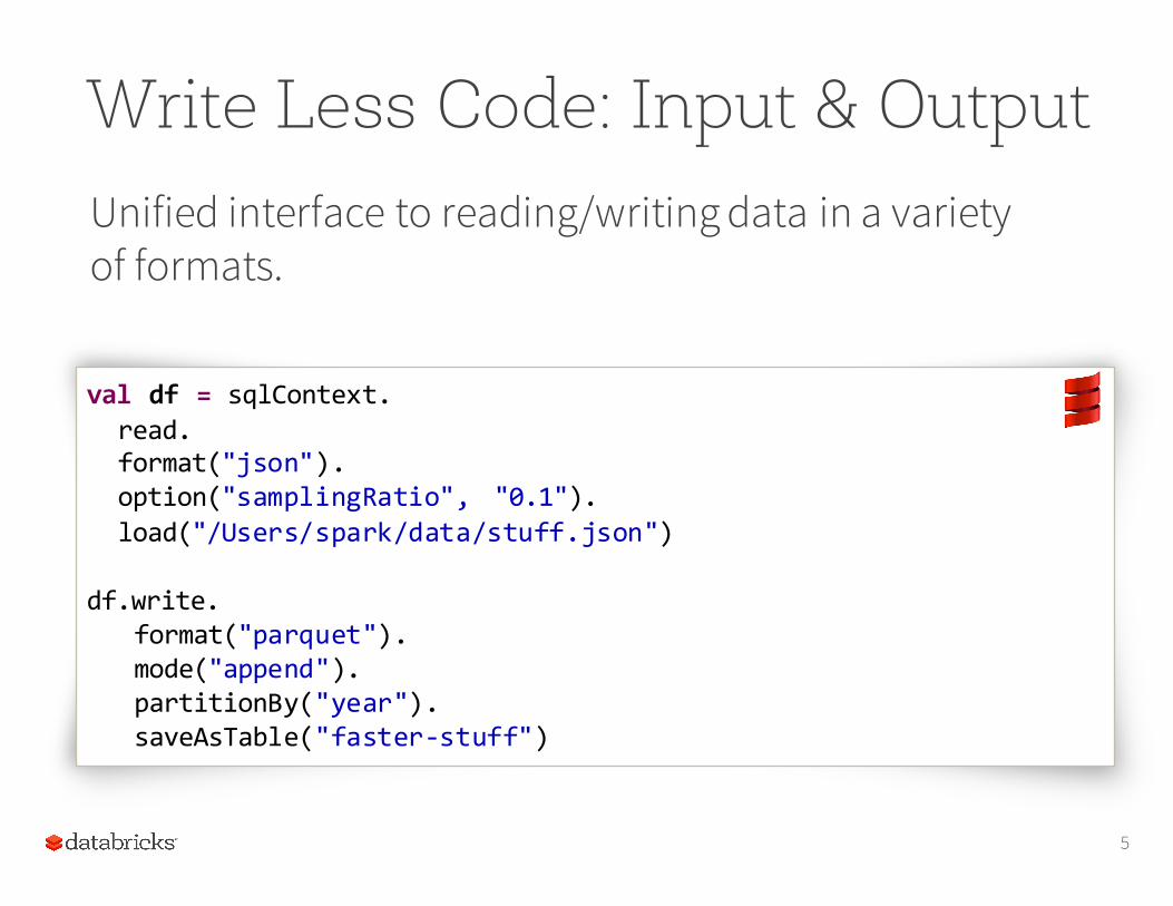
Write Less Code: Input & OutputUnified interface to reading/writing data in a variety of formats.
5
val df = sqlContext.read.format("json").option("samplingRatio", "0.1").load("/Users/spark/data/stuff.json")
df.write.format("parquet").mode("append").partitionBy("year").saveAsTable("faster-‐stuff")
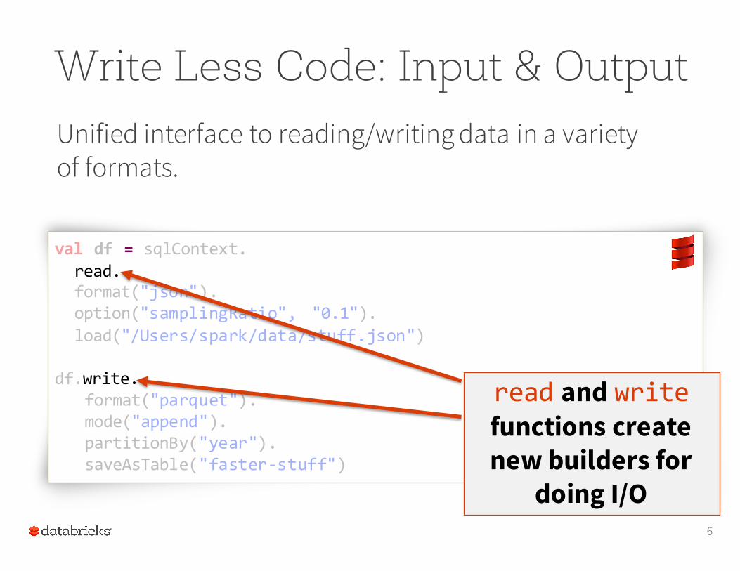
Write Less Code: Input & OutputUnified interface to reading/writing data in a variety of formats.
6
val df = sqlContext.read.format("json").option("samplingRatio", "0.1").load("/Users/spark/data/stuff.json")
df.write.format("parquet").mode("append").partitionBy("year").saveAsTable("faster-‐stuff")
read and writefunctions create new builders for
doing I/O
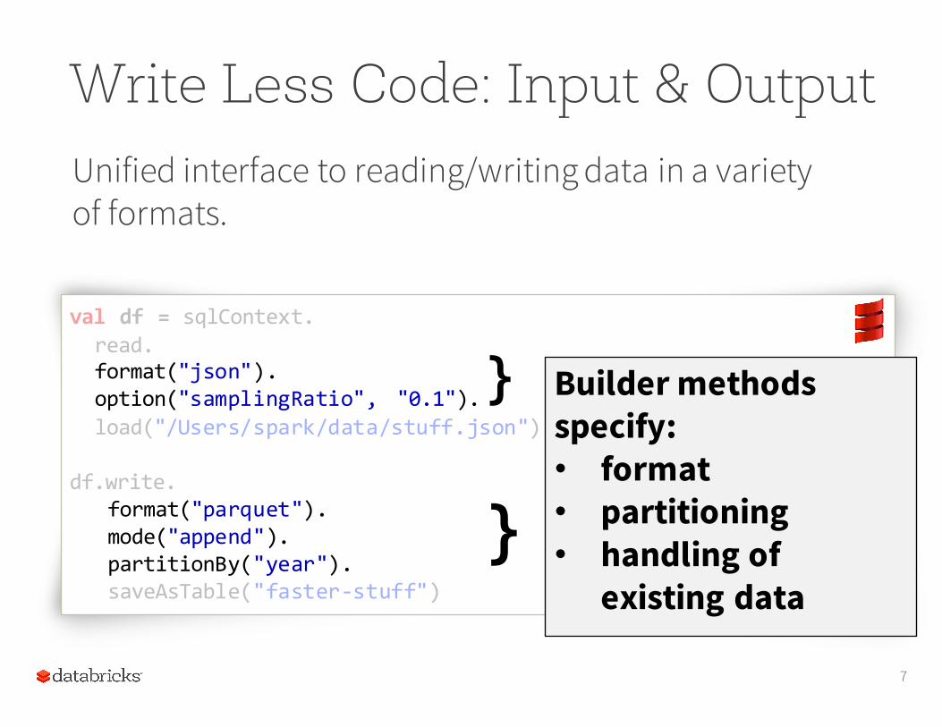
Write Less Code: Input & OutputUnified interface to reading/writing data in a variety of formats.
7
val df = sqlContext.read.format("json").option("samplingRatio", "0.1").load("/Users/spark/data/stuff.json")
df.write.format("parquet").mode("append").partitionBy("year").saveAsTable("faster-‐stuff")
Builder methodsspecify:• format• partitioning• handling of
existing data
}
}
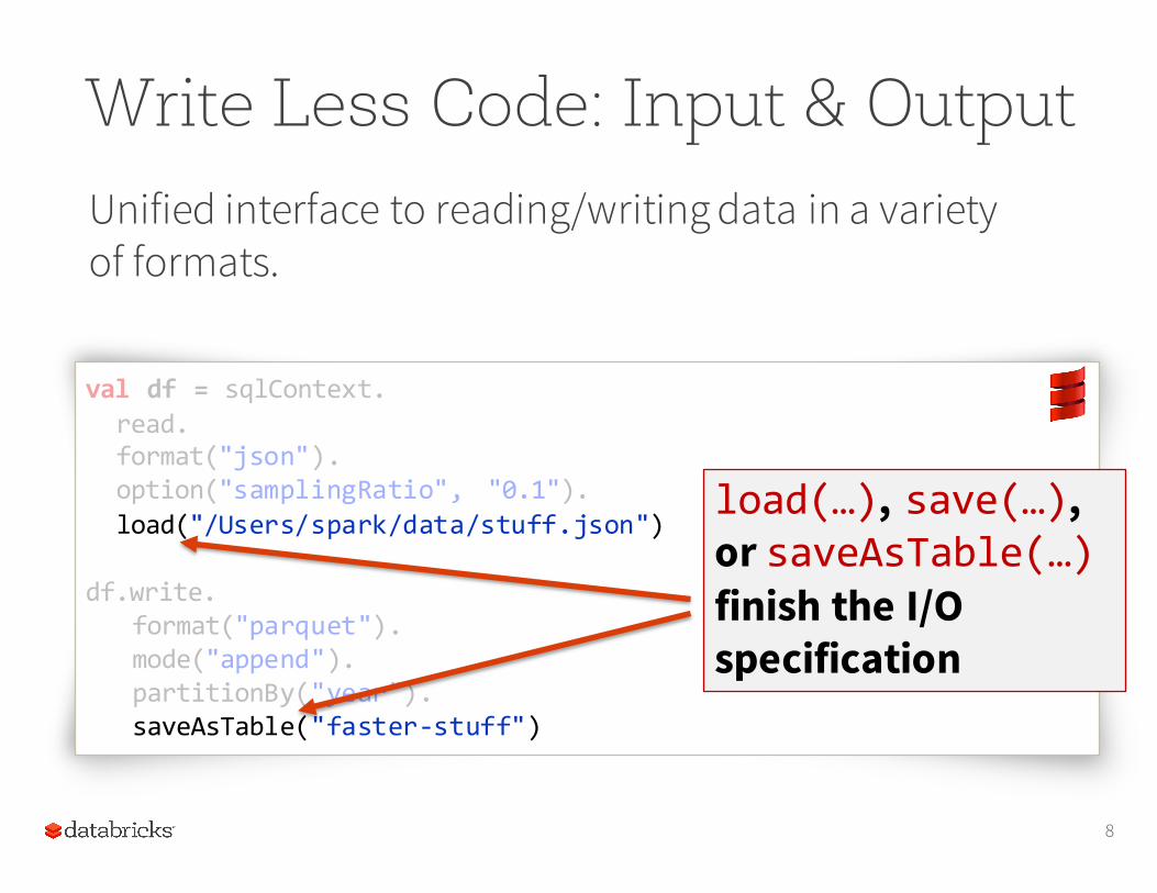
Write Less Code: Input & OutputUnified interface to reading/writing data in a variety of formats.
8
val df = sqlContext.read.format("json").option("samplingRatio", "0.1").load("/Users/spark/data/stuff.json")
df.write.format("parquet").mode("append").partitionBy("year").saveAsTable("faster-‐stuff")
load(…), save(…), or saveAsTable(…)finish the I/O specification
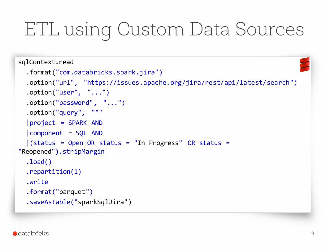
ETL using Custom Data SourcessqlContext.read
.format("com.databricks.spark.jira")
.option("url", "https://issues.apache.org/jira/rest/api/latest/search")
.option("user", "...")
.option("password", "...")
.option("query", """|project = SPARK AND|component = SQL AND|(status = Open OR status = "In Progress" OR status =
"Reopened").stripMargin.load().repartition(1).write.format("parquet").saveAsTable("sparkSqlJira")
9
Write Less Code: High-Level Operations
Solve common problems concisely using DataFramefunctions:
• selecting columns and filtering• joining different data sources• aggregation (count, sum, average, etc.)•plotting results (e.g., with Pandas)
10
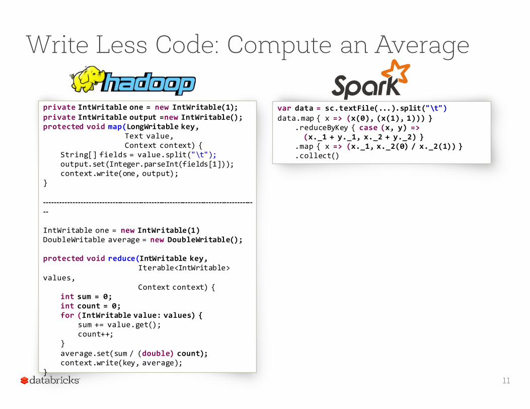
Write Less Code: Compute an Average
11
private IntWritable one = new IntWritable(1);private IntWritable output =new IntWritable();protected void map(LongWritable key,
Text value,Context context) {
String[] fields = value.split("\t");output.set(Integer.parseInt(fields[1]));context.write(one, output);
}
----------------------------------------------------------------------------------
IntWritable one = new IntWritable(1)DoubleWritable average = new DoubleWritable();
protected void reduce(IntWritable key,Iterable<IntWritable>
values,Context context) {
int sum = 0;int count = 0;for (IntWritable value: values) {
sum += value.get();count++;
}average.set(sum / (double) count);context.write(key, average);
}
var data = sc.textFile(...).split("\t")data.map { x => (x(0), (x(1), 1))) }
.reduceByKey { case (x, y) => (x._1 + y._1, x._2 + y._2) }
.map { x => (x._1, x._2(0) / x._2(1)) }
.collect()
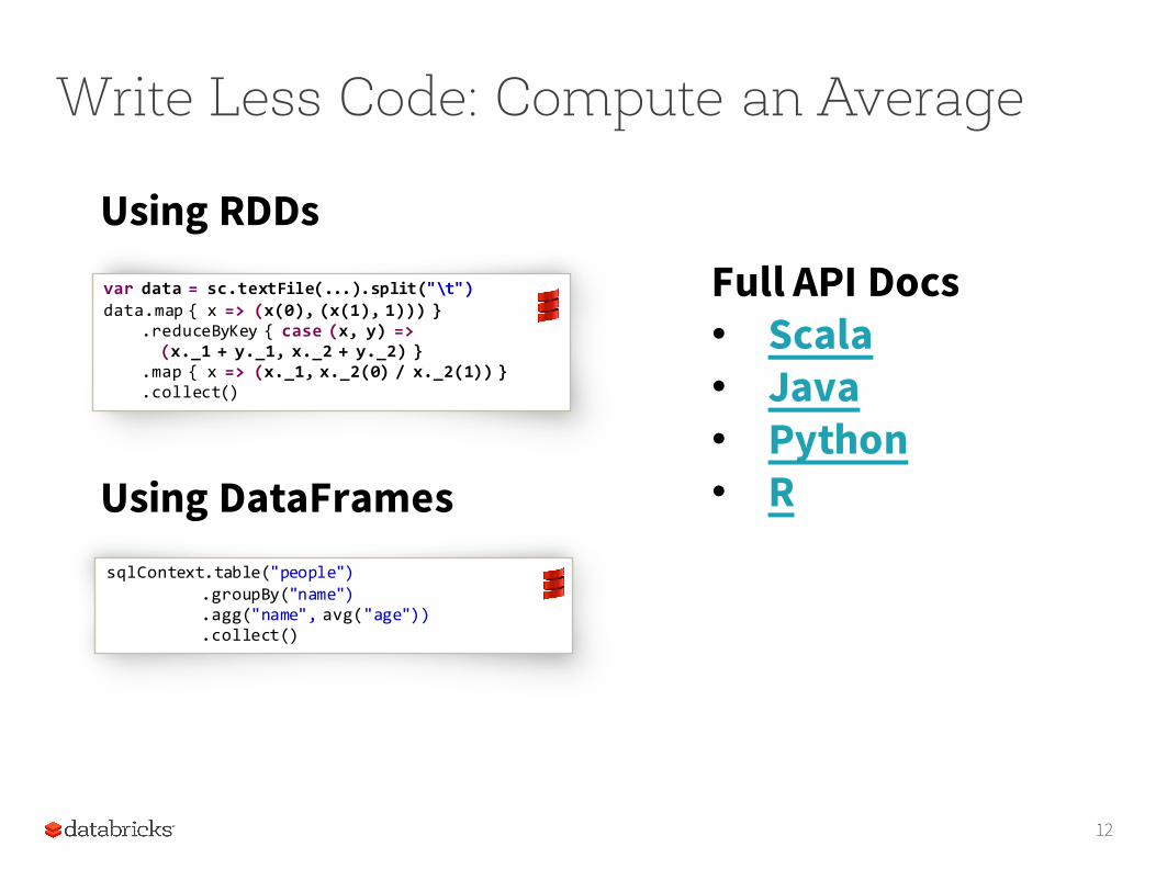
Write Less Code: Compute an Average
12
var data = sc.textFile(...).split("\t")data.map { x => (x(0), (x(1), 1))) }
.reduceByKey { case (x, y) => (x._1 + y._1, x._2 + y._2) }
.map { x => (x._1, x._2(0) / x._2(1)) }
.collect()
Using RDDs
Using DataFramessqlContext.table("people")
.groupBy("name")
.agg("name", avg("age"))
.collect()
Full API Docs• Scala• Java• Python• R
What are DataFrames?DataFrames are a recent addition to Spark (early 2015).
The DataFrames API:
• is intended to enable wider audiences beyond “Big Data” engineers to leverage the power of distributed processing• is inspired by data frames in R and Python (Pandas)• designed from the ground-up to support modern big
data and data science applications• an extension to the existing RDD API
See databricks.com/blog/2015/02/17/introducing-dataframes-in-spark-for-large-scale-data-science.html
13
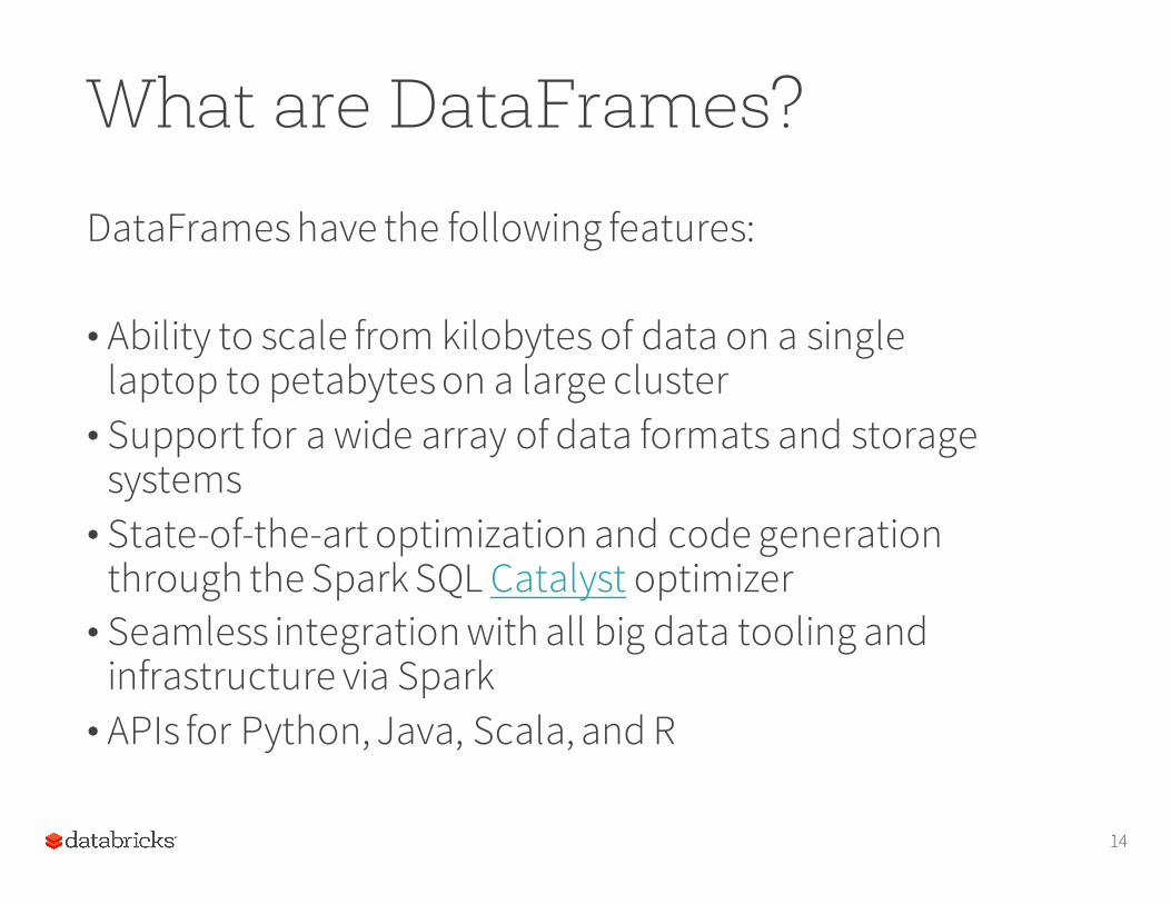
What are DataFrames?
DataFrames have the following features:
• Ability to scale from kilobytes of data on a single laptop to petabytes on a large cluster• Support for a wide array of data formats and storage
systems• State-of-the-art optimization and code generation
through the Spark SQL Catalyst optimizer• Seamless integration with all big data tooling and
infrastructure via Spark• APIs for Python, Java, Scala, and R
14

What are DataFrames?
• For new users familiar with data frames in other programming languages, this API should make them feel at home. • For existing Spark users, the API will make Spark
easier to program.• For both sets of users, DataFrames will improve
performance through intelligent optimizations and code-generation.
15
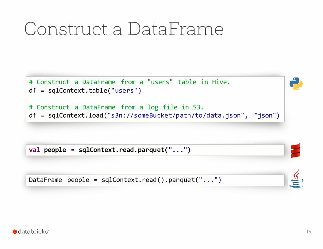
Construct a DataFrame
16
# Construct a DataFrame from a "users" table in Hive.df = sqlContext.table("users")
# Construct a DataFrame from a log file in S3.df = sqlContext.load("s3n://someBucket/path/to/data.json", "json")
val people = sqlContext.read.parquet("...")
DataFrame people = sqlContext.read().parquet("...")
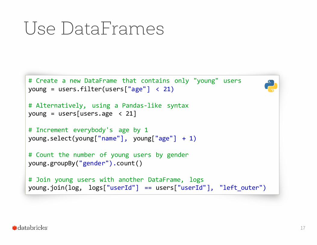
Use DataFrames
17
# Create a new DataFrame that contains only "young" usersyoung = users.filter(users["age"] < 21)
# Alternatively, using a Pandas-‐like syntaxyoung = users[users.age < 21]
# Increment everybody's age by 1young.select(young["name"], young["age"] + 1)
# Count the number of young users by genderyoung.groupBy("gender").count()
# Join young users with another DataFrame, logsyoung.join(log, logs["userId"] == users["userId"], "left_outer")
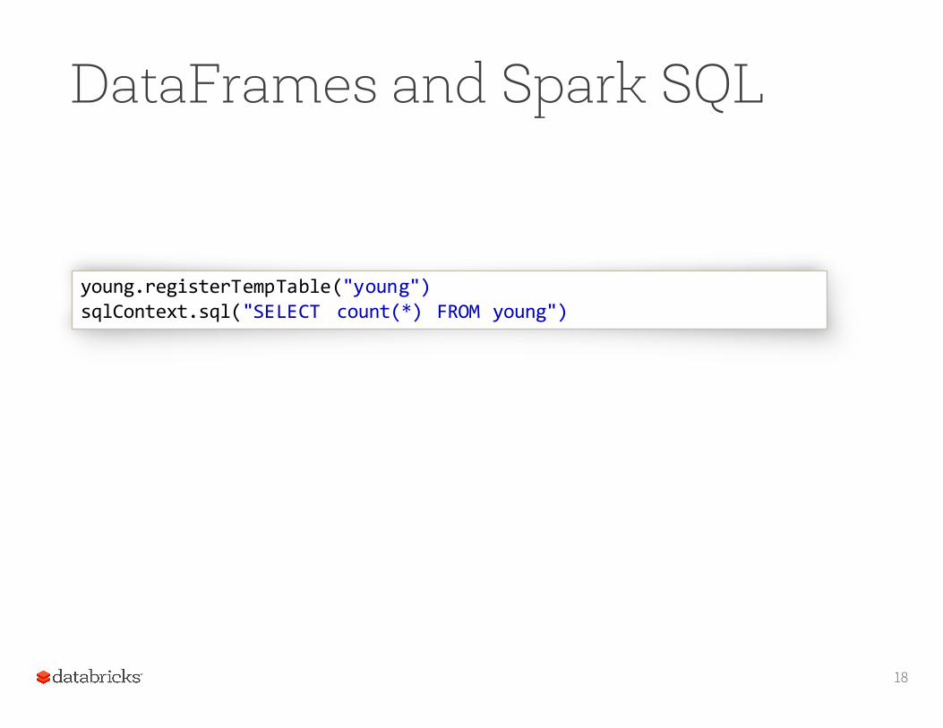
DataFrames and Spark SQL
18
young.registerTempTable("young")sqlContext.sql("SELECT count(*) FROM young")
More details, coming up
We will be looking at DataFrame operations in more detail shortly.
19
DataFrames and Spark SQL
DataFrames are fundamentally tied to Spark SQL.•The DataFrames API provides a programmatic
interface—really, a domain-specific language(DSL)—for interacting with your data.•Spark SQL provides a SQL-like interface.•What you can do in Spark SQL, you can do in
DataFrames•… and vice versa.
20

What, exactly, is Spark SQL?
Spark SQL allows you to manipulate distributed data with SQL queries. Currently, two SQL dialects are supported.• If you're using a Spark SQLContext, the only
supported dialect is "sql", a rich subset of SQL 92.• If you're using a HiveContext, the default dialect
is "hiveql", corresponding to Hive's SQL dialect. "sql" is also available, but "hiveql" is a richer dialect.
21
Spark SQL
• You issue SQL queries through a SQLContext or HiveContext, using the sql() method.•The sql() method returns a DataFrame.• You can mix DataFrame methods and SQL queries
in the same code.•To use SQL, you must either:• query a persisted Hive table, or• make a table alias for a DataFrame, using registerTempTable()
22
DataFrames
Like Spark SQL, the DataFrames API assumes that the data has a table-like structure.
Formally, a DataFrame is a size-mutable, potentially heterogeneous tabular data structure with labeled axes (i.e., rows and columns).
That’s a mouthful. Just think of it as a table in a distributed database: a distributed collection of data organized into named, typed columns.
23
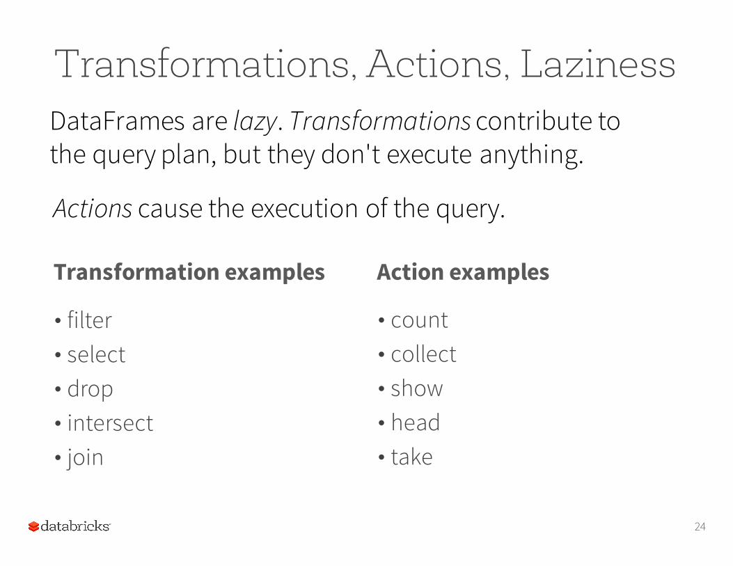
Transformation examples Action examples
Transformations, Actions, Laziness
• count• collect• show• head• take
• filter• select• drop• intersect• join
24
DataFrames are lazy. Transformations contribute to the query plan, but they don't execute anything.
Actions cause the execution of the query.
Transformations, Actions, LazinessActions cause the execution of the query.
What, exactly does "execution of the query" mean?It means:•Spark initiates a distributed read of the data
source•The data flows through the transformations (the
RDDs resulting from the Catalyst query plan)•The result of the action is pulled back into the
driver JVM.
25
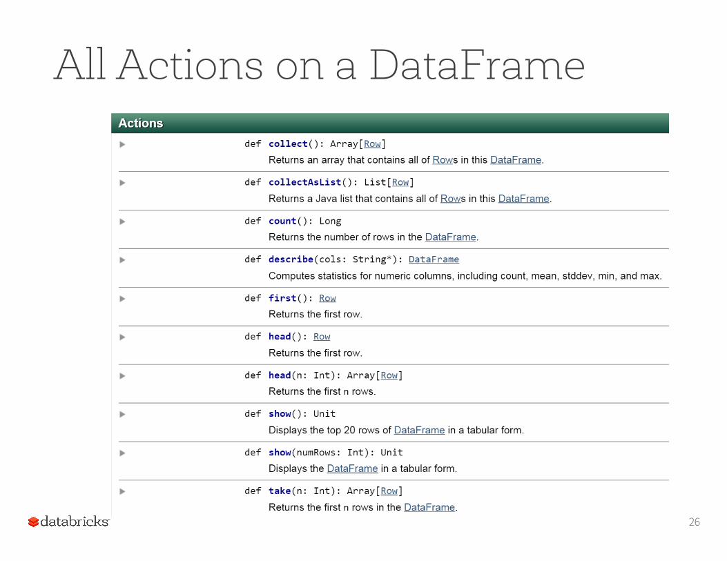
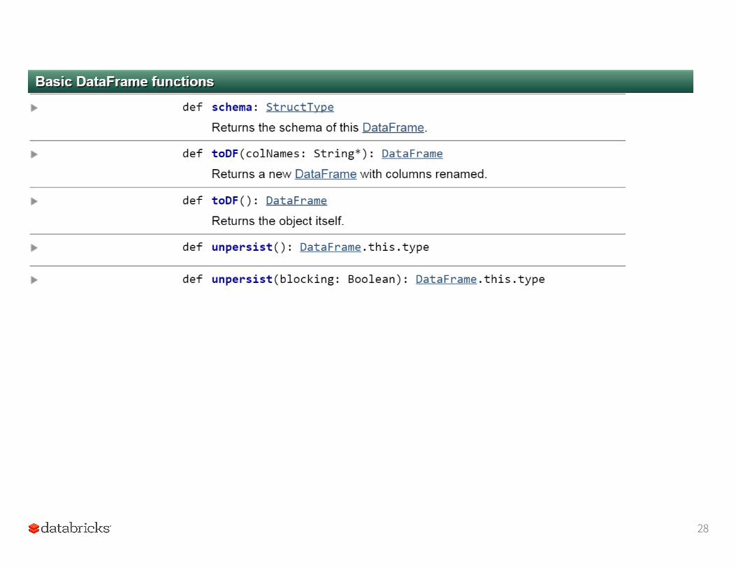
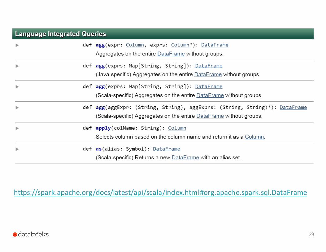
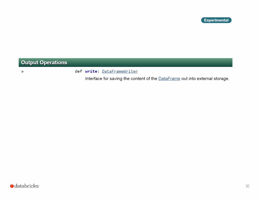
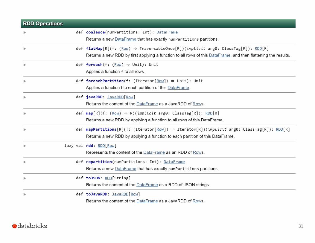
All Actions on a DataFrame
26
27
28
29
https://spark.apache.org/docs/latest/api/scala/index.html#org.apache.spark.sql.DataFrame
30
31
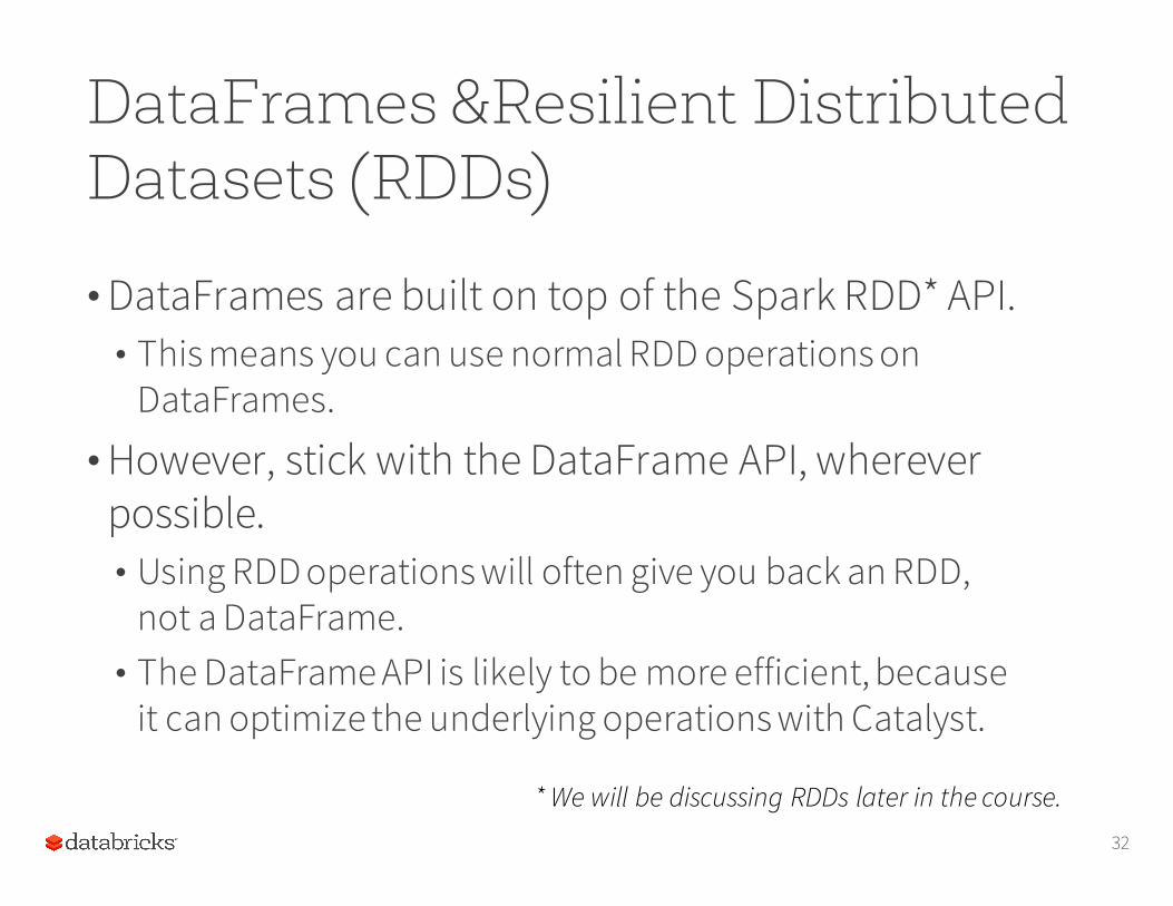
DataFrames &Resilient Distributed Datasets (RDDs)
•DataFrames are built on top of the Spark RDD* API.• This means you can use normal RDD operations on
DataFrames.
•However, stick with the DataFrame API, wherever possible.• Using RDD operations will often give you back an RDD,
not a DataFrame.• The DataFrame API is likely to be more efficient, because
it can optimize the underlying operations with Catalyst.
32
* We will be discussing RDDs later in the course.
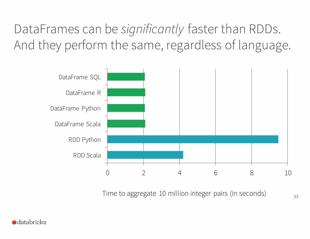
DataFrames can be significantly faster than RDDs. And they perform the same, regardless of language.
33
0 2 4 6 8 10
RDD Scala
RDD Python
DataFrame Scala
DataFrame Python
DataFrame R
DataFrame SQL
Time to aggregate 10 million integer pairs (in seconds)
Plan Optimization & Execution
•Represented internally as a “logical plan”•Execution is lazy, allowing it to be optimized by
Catalyst
34
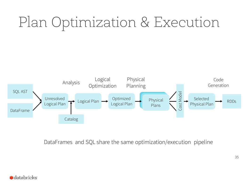
Plan Optimization & Execution
35
SQL AST
DataFrame
Unresolved Logical Plan Logical Plan Optimized
Logical Plan RDDsSelected Physical Plan
Analysis LogicalOptimization
PhysicalPlanning
Cost
Mod
el
Physical Plans
CodeGeneration
Catalog
DataFrames and SQL share the same optimization/execution pipeline
36
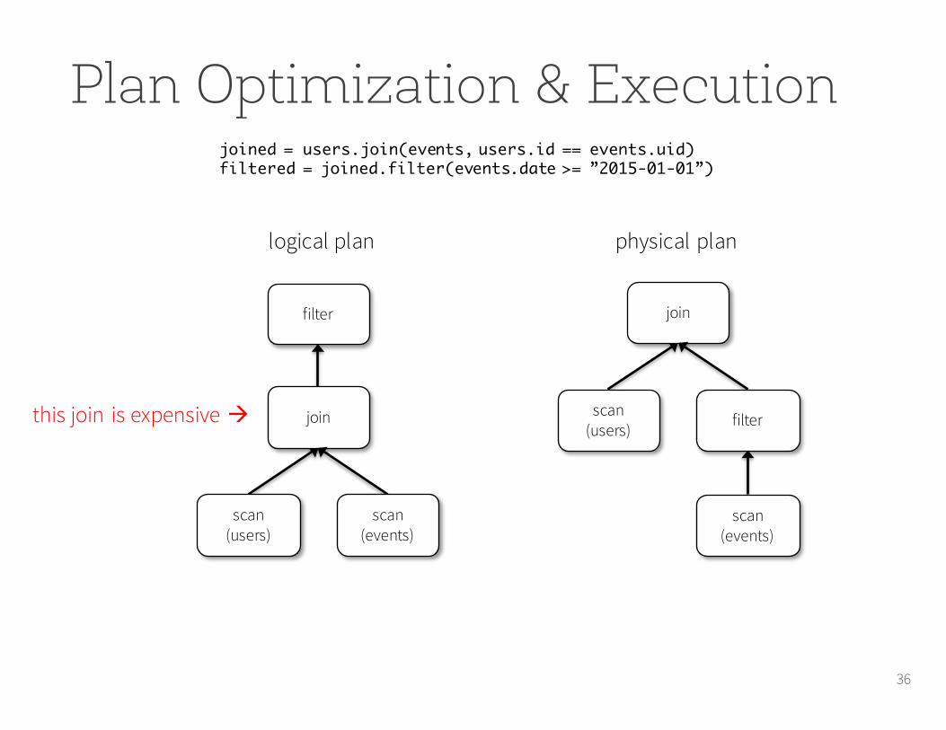
joined = users.join(events, users.id == events.uid)filtered = joined.filter(events.date >= ”2015-01-01”)
logical plan
filter
join
scan(users)
scan(events)
physical plan
join
scan(users) filter
scan(events)
this join is expensive à
Plan Optimization & Execution
Plan Optimization: "Intelligent" Data Sources
The Data Sources API can automatically prune columns and push filters to the source
•Parquet: skip irrelevant columns and blocks of data; turn string comparison into integer comparisons for dictionary encoded data
• JDBC: Rewrite queries to push predicates down37
38
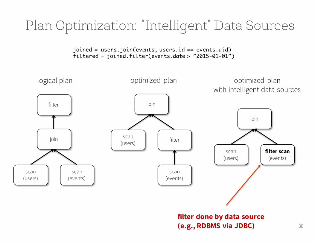
joined = users.join(events, users.id == events.uid)filtered = joined.filter(events.date > ”2015-01-01”)
logical plan
filter
join
scan(users)
scan(events)
optimized plan
join
scan(users) filter
scan(events)
optimized planwith intelligent data sources
join
scan(users)
filter scan(events)
Plan Optimization: "Intelligent" Data Sources
filter done by data source (e.g., RDBMS via JDBC)
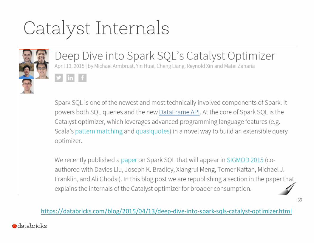
Catalyst Internals
39
https://databricks.com/blog/2015/04/13/deep-‐dive-‐into-‐spark-‐sqls-‐catalyst-‐optimizer.html

3 Fundamental transformations on DataFrames
40
- mapPartitions- New ShuffledRDD- ZipPartitions
DataFrame limitations
41
•Catalyst does not automatically repartition DataFramesoptimally
•During a DF shuffle, Spark SQL will just use spark.sql.shuffle.partitions to determine the number of partitions in the downstream RDD
•All SQL configurations can be changed via sqlContext.setConf(key, value) or in DB: "%sql SET key=val"
Creating a DataFrame
• You create a DataFrame with a SQLContextobject (or one of its descendants)• In the Spark Scala shell (spark-shell) or pyspark,
you have a SQLContext available automatically, as sqlContext.• In an application, you can easily create one
yourself, from a SparkContext.•The DataFrame data source API is consistent,
across data formats. • “Opening” a data source works pretty much the same
way, no matter what.
42
Creating a DataFrame in Scala
43
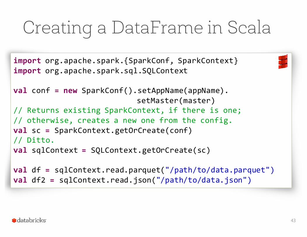
import org.apache.spark.{SparkConf, SparkContext}import org.apache.spark.sql.SQLContext
val conf = new SparkConf().setAppName(appName).setMaster(master)
// Returns existing SparkContext, if there is one;// otherwise, creates a new one from the config.val sc = SparkContext.getOrCreate(conf)// Ditto.val sqlContext = SQLContext.getOrCreate(sc)
val df = sqlContext.read.parquet("/path/to/data.parquet")val df2 = sqlContext.read.json("/path/to/data.json")
Creating a DataFrame in Python
44
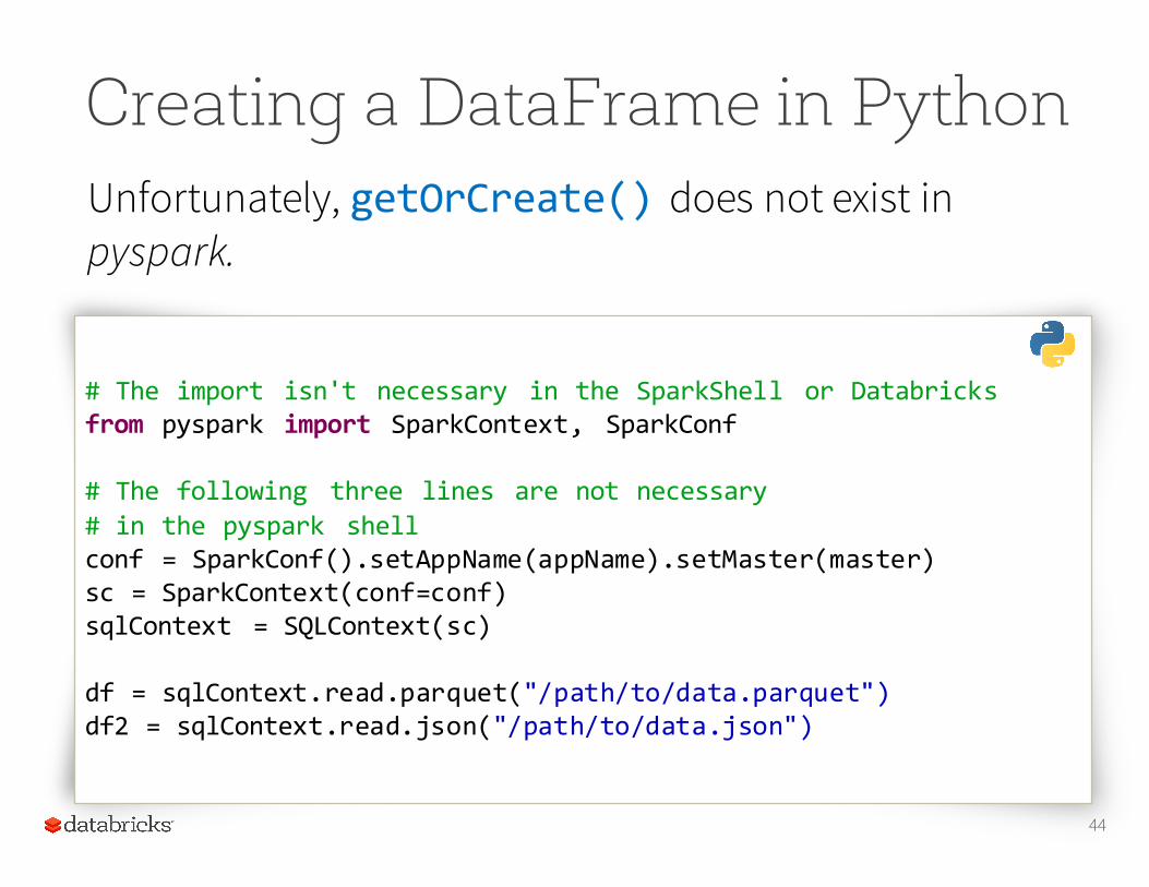
# The import isn't necessary in the SparkShell or Databricksfrom pyspark import SparkContext, SparkConf
# The following three lines are not necessary# in the pyspark shellconf = SparkConf().setAppName(appName).setMaster(master)sc = SparkContext(conf=conf)sqlContext = SQLContext(sc)
df = sqlContext.read.parquet("/path/to/data.parquet")df2 = sqlContext.read.json("/path/to/data.json")
Unfortunately, getOrCreate() does not exist in pyspark.
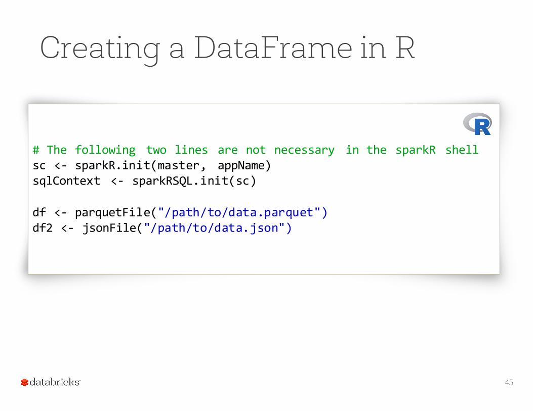
Creating a DataFrame in R
45
# The following two lines are not necessary in the sparkR shellsc <-‐ sparkR.init(master, appName)sqlContext <-‐ sparkRSQL.init(sc)
df <-‐ parquetFile("/path/to/data.parquet")df2 <-‐ jsonFile("/path/to/data.json")
SQLContext and HiveOur previous examples created a default Spark SQLContext object.
If you're using a version of Spark that has Hive support, you can also create aHiveContext, which provides additional features, including:
• the ability to write queries using the more complete HiveQL parser• access to Hive user-defined functions• the ability to read data from Hive tables.
46
HiveContext
•To use a HiveContext, you do not need to have an existing Hive installation, and all of the data sources available to a SQLContext are still available.• You do, however, need to have a version of Spark that
was built with Hive support. That's not the default.• Hive is packaged separately to avoid including all of Hive’s
dependencies in the default Spark build. • If these dependencies are not a problem for your application
then using HiveContext is currently recommended.
• It's not difficult to build Spark with Hive support.
47
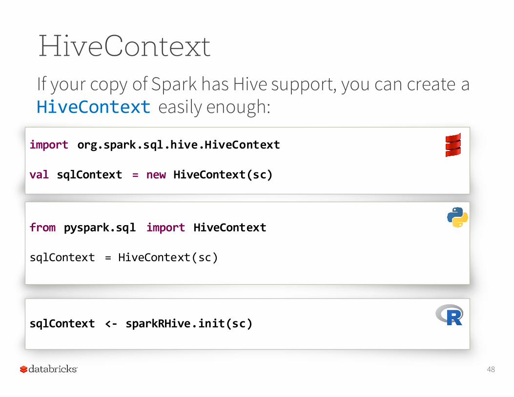
HiveContextIf your copy of Spark has Hive support, you can create a HiveContext easily enough:
48
import org.spark.sql.hive.HiveContext
val sqlContext = new HiveContext(sc)
from pyspark.sql import HiveContext
sqlContext = HiveContext(sc)
sqlContext <-‐ sparkRHive.init(sc)
DataFrames Have SchemasIn the previous example, we created DataFrames from Parquet and JSON data.•A Parquet table has a schema (column names and
types) that Spark can use. Parquet also allows Spark to be efficient about how it pares down data.•Spark can infer a Schema from a JSON file.
49
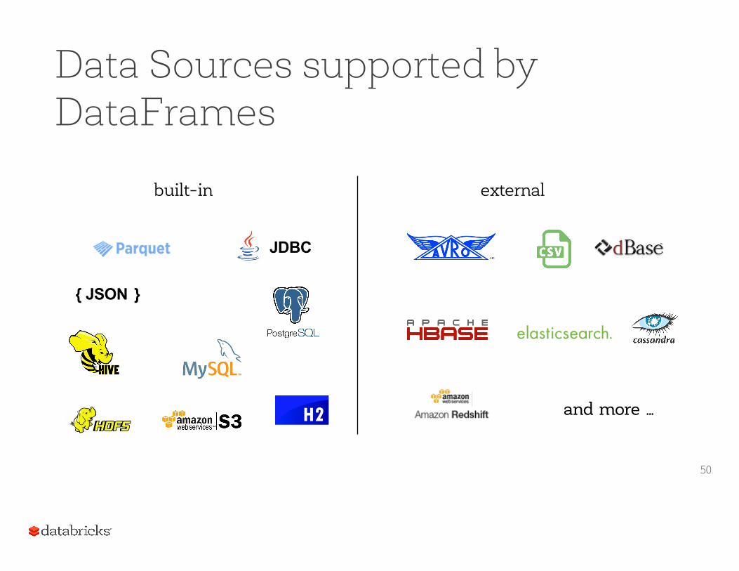
Data Sources supported by DataFrames
50
{ JSON }
built-in external
JDBC
and more …
Schema InferenceWhat if your data file doesn’t have a schema? (e.g., You’re reading a CSV file or a plain text file.)
• You can create an RDD of a particular type and let Spark infer the schema from that type. We’ll see how to do that in a moment.• You can use the API to specify the schema
programmatically.
(It’s better to use a schema-oriented input source if you can, though.)
51
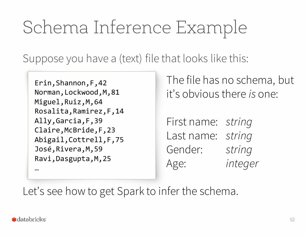
Schema Inference ExampleSuppose you have a (text) file that looks like this:
52
The file has no schema, but it’s obvious there is one:
First name: stringLast name: stringGender: stringAge: integer
Let’s see how to get Spark to infer the schema.
Erin,Shannon,F,42Norman,Lockwood,M,81Miguel,Ruiz,M,64Rosalita,Ramirez,F,14Ally,Garcia,F,39Claire,McBride,F,23Abigail,Cottrell,F,75José,Rivera,M,59Ravi,Dasgupta,M,25…
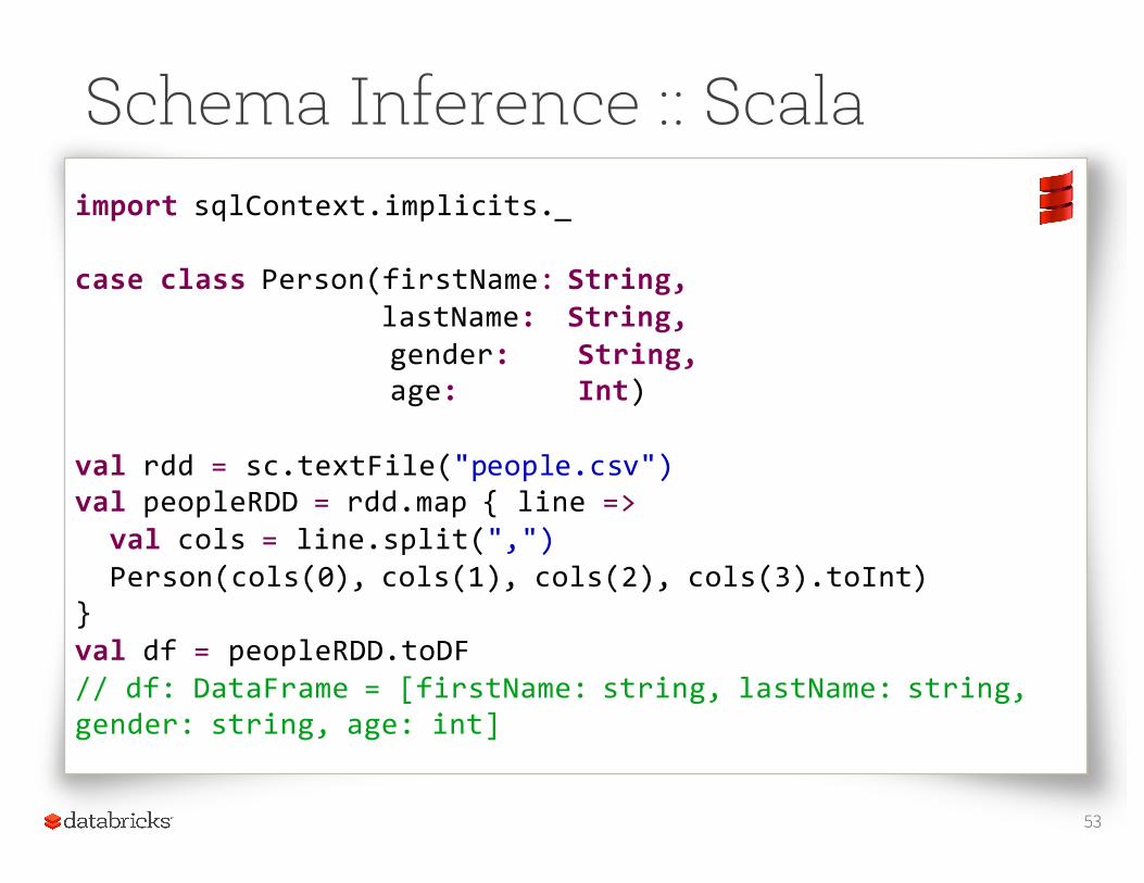
Schema Inference :: Scala
53
import sqlContext.implicits._
case class Person(firstName: String,lastName: String,gender: String,age: Int)
val rdd = sc.textFile("people.csv")val peopleRDD = rdd.map { line =>
val cols = line.split(",")Person(cols(0), cols(1), cols(2), cols(3).toInt)
}val df = peopleRDD.toDF// df: DataFrame = [firstName: string, lastName: string, gender: string, age: int]
Schema Inference :: Python
•We can do the same thing in Python.•Use a namedtuple, dict, or Row, instead of a
Python class, though.*• Row is part of the DataFrames API
* Seespark.apache.org/docs/latest/api/python/pyspark.sql.html#pyspark.sql.SQLContext.createDataFrame
54
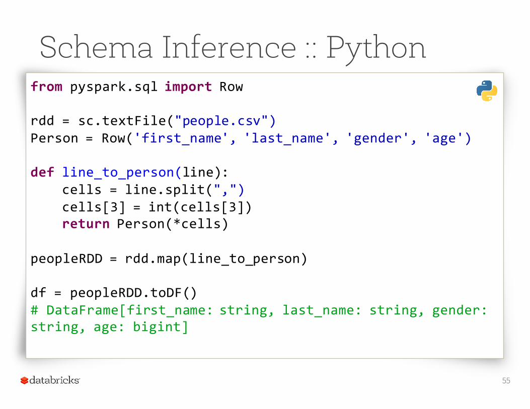
Schema Inference :: Python
55
from pyspark.sql import Row
rdd = sc.textFile("people.csv")Person = Row('first_name', 'last_name', 'gender', 'age')
def line_to_person(line):cells = line.split(",")cells[3] = int(cells[3])return Person(*cells)
peopleRDD = rdd.map(line_to_person)
df = peopleRDD.toDF()# DataFrame[first_name: string, last_name: string, gender: string, age: bigint]
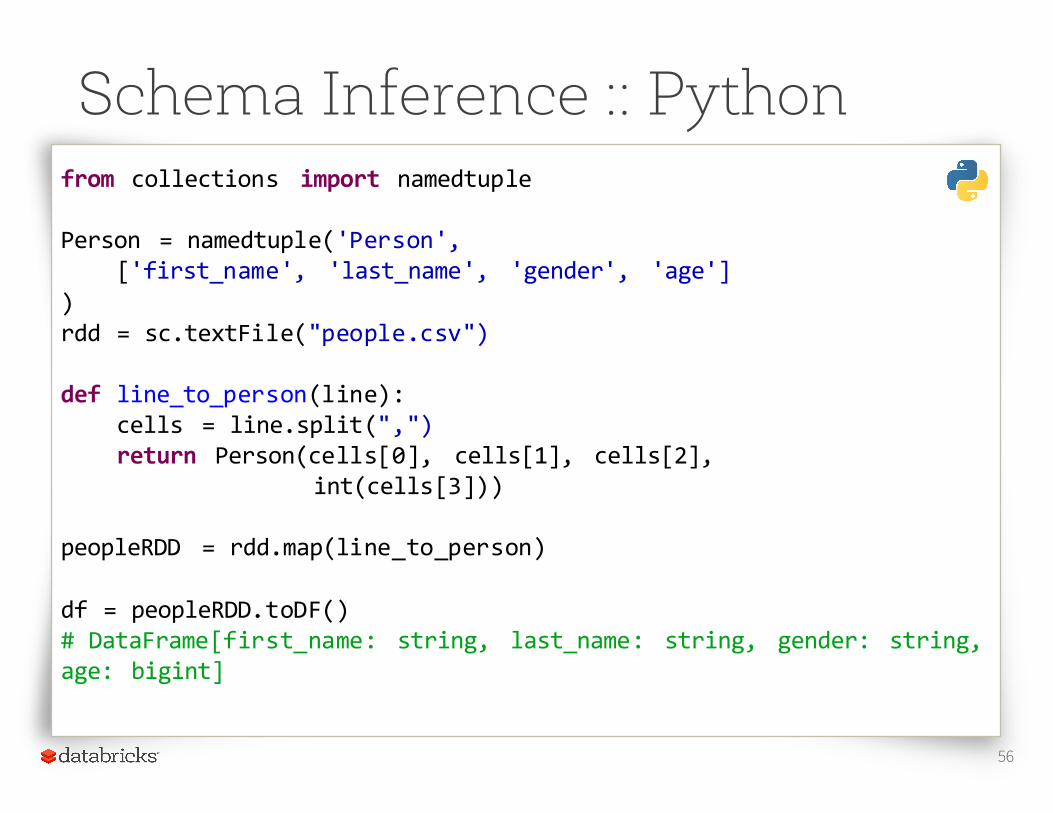
Schema Inference :: Python
56
from collections import namedtuple
Person = namedtuple('Person',['first_name', 'last_name', 'gender', 'age']
)rdd = sc.textFile("people.csv")
def line_to_person(line):cells = line.split(",")return Person(cells[0], cells[1], cells[2],
int(cells[3]))
peopleRDD = rdd.map(line_to_person)
df = peopleRDD.toDF()# DataFrame[first_name: string, last_name: string, gender: string, age: bigint]
Schema Inference
We can also force schema inference without creating our own People type, by using a fixed-length data structure (such as a tuple) and supplying the column names to the toDF()method.
57
Schema Inference :: Scala
58
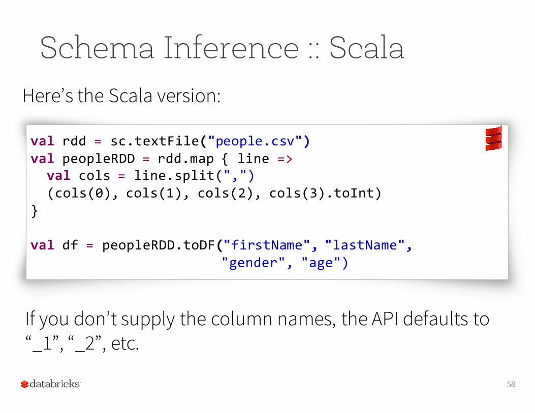
If you don’t supply the column names, the API defaults to “_1”, “_2”, etc.
val rdd = sc.textFile("people.csv")val peopleRDD = rdd.map { line =>
val cols = line.split(",")(cols(0), cols(1), cols(2), cols(3).toInt)
}
val df = peopleRDD.toDF("firstName", "lastName","gender", "age")
Here’s the Scala version:
Schema Inference :: Python
59
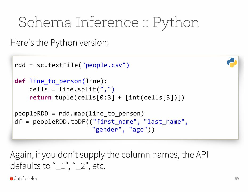
Again, if you don’t supply the column names, the API defaults to “_1”, “_2”, etc.
Here’s the Python version:
rdd = sc.textFile("people.csv")
def line_to_person(line):cells = line.split(",")return tuple(cells[0:3] + [int(cells[3])])
peopleRDD = rdd.map(line_to_person)df = peopleRDD.toDF(("first_name", "last_name",
"gender", "age"))
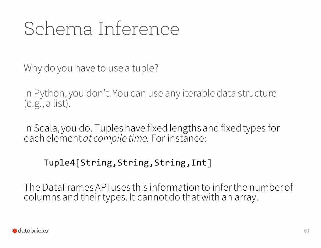
Why do you have to use a tuple?
In Python, you don’t. You can use any iterable data structure (e.g., a list).
In Scala, you do. Tuples have fixed lengths and fixed types for each element at compile time. For instance:
Tuple4[String,String,String,Int]
The DataFrames API uses this information to infer the number of columns and their types. It cannot do that with an array.
Schema Inference
60
Hands OnIn the labs area of the shard, under the sql-‐and-‐dataframes folder, you'll find another folder called hands-‐on.
Within that folder are two notebooks, Scala and Python.
• Clone one of those notebooks into your home folder.• Open it.• Attach it to a cluster.
We're going to walk through the first section, entitled Schema Inference.
61
Additional Input Formats
The DataFrames API can be extended to understand additional input formats (or, input sources).
For instance, if you’re dealing with CSV files, a verycommon data file format, you can use the spark-csvpackage (spark-packages.org/package/databricks/spark-csv)
This package augments the DataFrames API so that it understands CSV files.
62
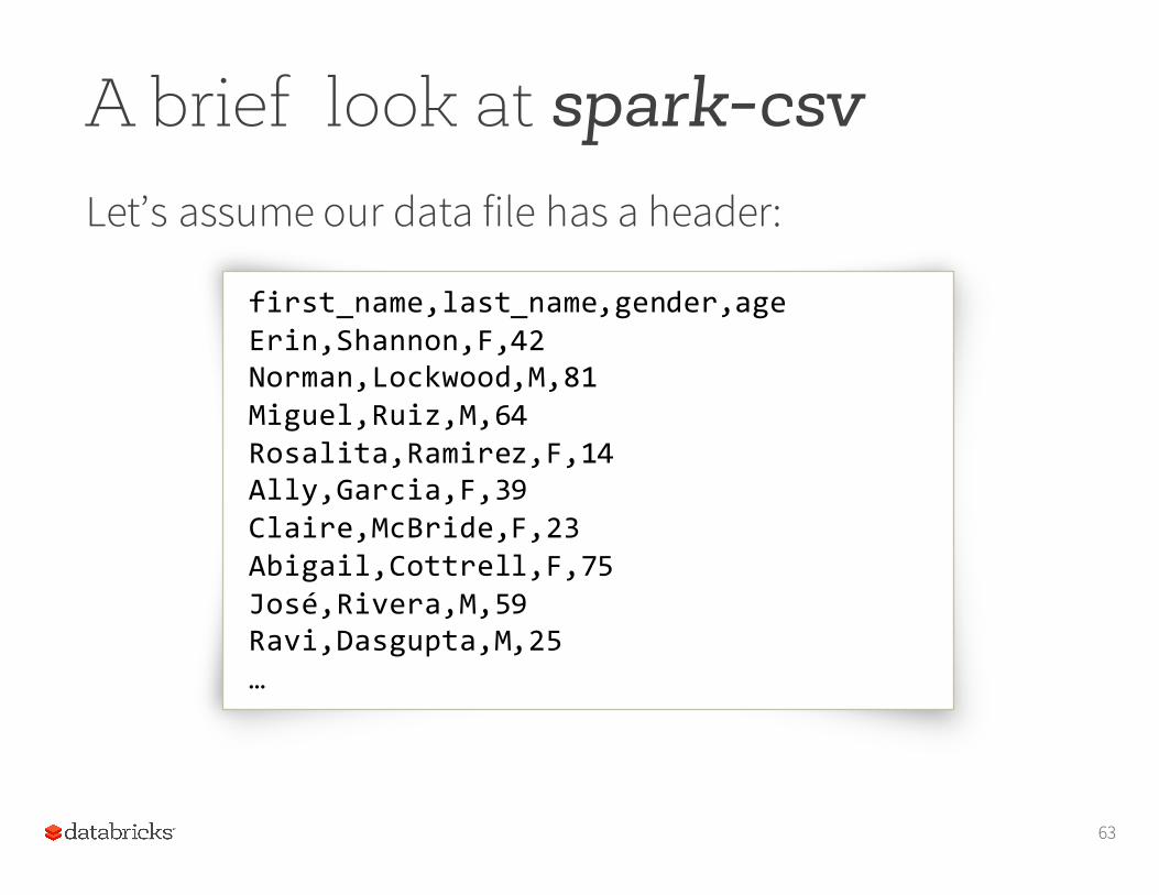
A brief look at spark-csvLet’s assume our data file has a header:
63
first_name,last_name,gender,ageErin,Shannon,F,42Norman,Lockwood,M,81Miguel,Ruiz,M,64Rosalita,Ramirez,F,14Ally,Garcia,F,39Claire,McBride,F,23Abigail,Cottrell,F,75José,Rivera,M,59Ravi,Dasgupta,M,25…
A brief look at spark-csv
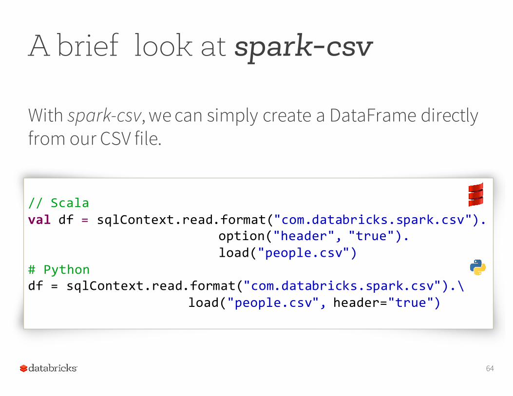
With spark-csv, we can simply create a DataFrame directly from our CSV file.
64
// Scalaval df = sqlContext.read.format("com.databricks.spark.csv").
option("header", "true").load("people.csv")
# Pythondf = sqlContext.read.format("com.databricks.spark.csv").\
load("people.csv", header="true")
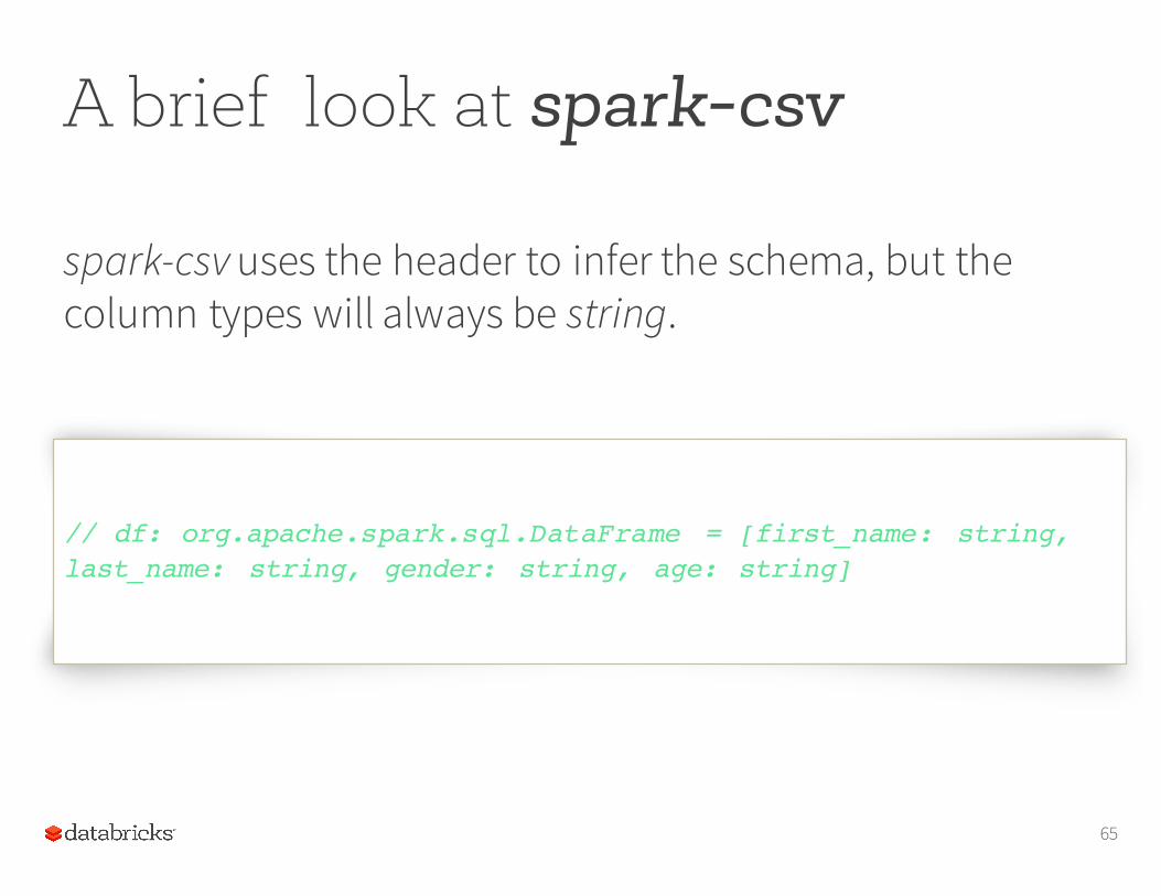
A brief look at spark-csv
65
spark-csv uses the header to infer the schema, but the column types will always be string.
// df: org.apache.spark.sql.DataFrame = [first_name: string, last_name: string, gender: string, age: string]
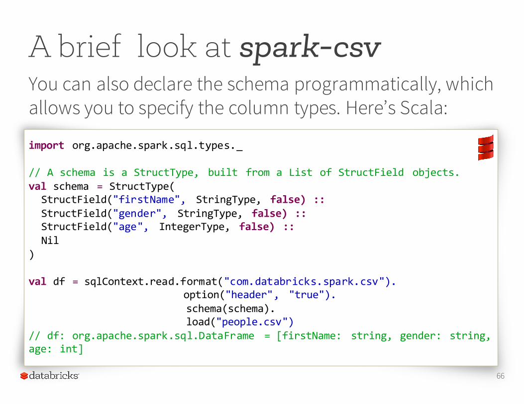
A brief look at spark-csvYou can also declare the schema programmatically, which allows you to specify the column types. Here’s Scala:
66
import org.apache.spark.sql.types._
// A schema is a StructType, built from a List of StructField objects.val schema = StructType(
StructField("firstName", StringType, false) ::StructField("gender", StringType, false) ::StructField("age", IntegerType, false) ::Nil
)
val df = sqlContext.read.format("com.databricks.spark.csv").option("header", "true").schema(schema).load("people.csv")
// df: org.apache.spark.sql.DataFrame = [firstName: string, gender: string, age: int]
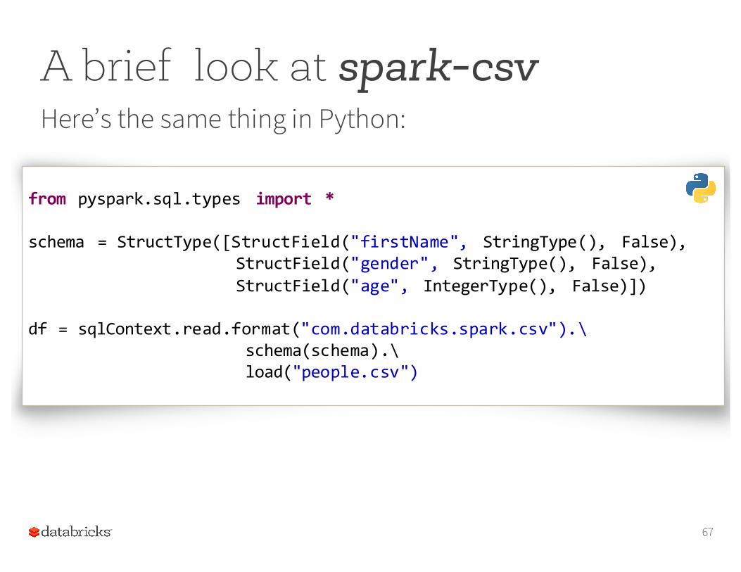
A brief look at spark-csvHere’s the same thing in Python:
67
from pyspark.sql.types import *
schema = StructType([StructField("firstName", StringType(), False),StructField("gender", StringType(), False),StructField("age", IntegerType(), False)])
df = sqlContext.read.format("com.databricks.spark.csv").\schema(schema).\load("people.csv")
What can I do with a DataFrame?
Once you have a DataFrame, there are a number of operations you can perform.
Let’s look at a few of them.
But, first, let’s talk about columns.
68
ColumnsWhen we say “column” here, what do we mean?
A DataFrame column is an abstraction. It provides a common column-oriented view of the underlying data, regardless of how the data is really organized.
69
Columns
70
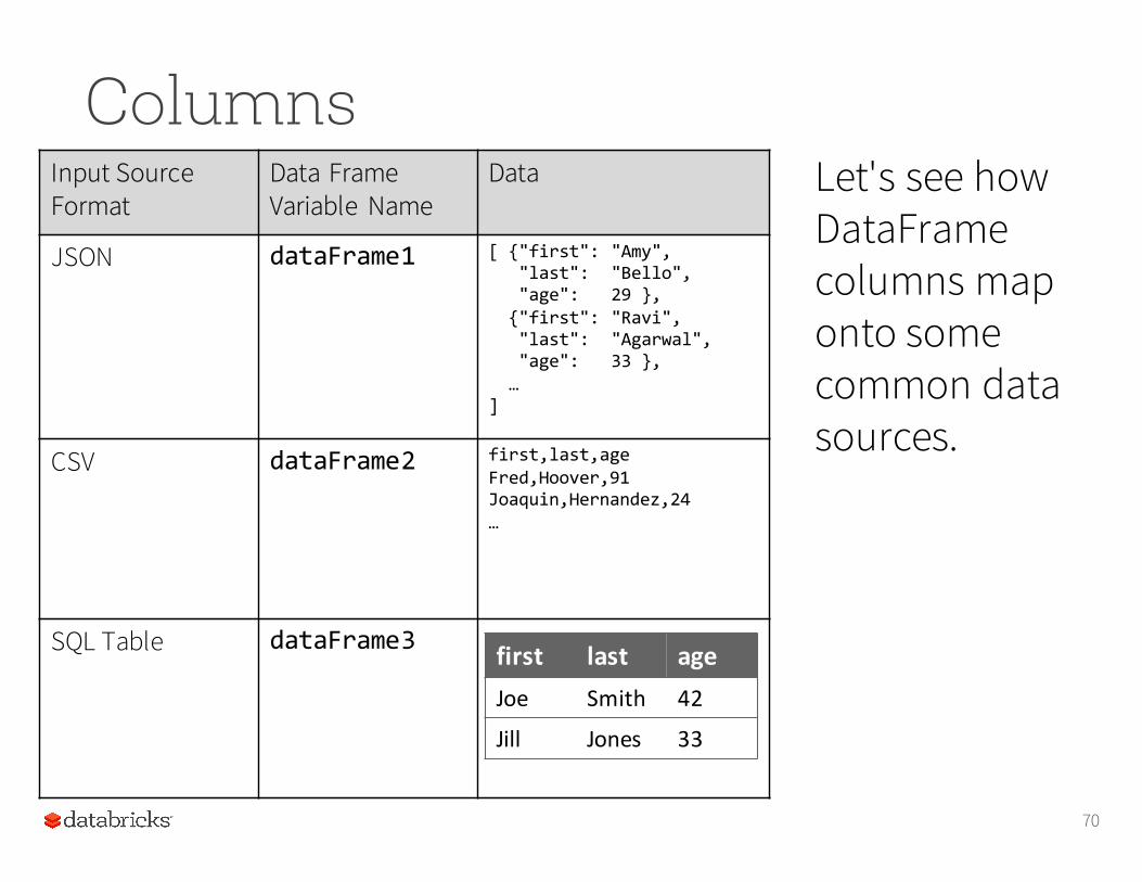
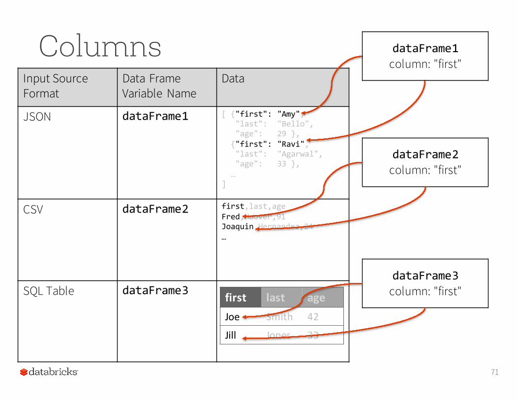
Let's see how DataFrame columns map onto some common data sources.
Input Source Format
Data Frame Variable Name
Data
JSON dataFrame1 [ {"first": "Amy","last": "Bello","age": 29 },{"first": "Ravi","last": "Agarwal","age": 33 },…
]
CSV dataFrame2 first,last,ageFred,Hoover,91Joaquin,Hernandez,24…
SQL Table dataFrame3 first last ageJoe Smith 42
Jill Jones 33
Columns
71
Input Source Format
Data Frame Variable Name
Data
JSON dataFrame1 [ {"first": "Amy","last": "Bello","age": 29 },{"first": "Ravi","last": "Agarwal","age": 33 },…
]
CSV dataFrame2 first,last,ageFred,Hoover,91Joaquin,Hernandez,24…
SQL Table dataFrame3 first last ageJoe Smith 42
Jill Jones 33
dataFrame1column: "first"
dataFrame2column: "first"
dataFrame3column: "first"
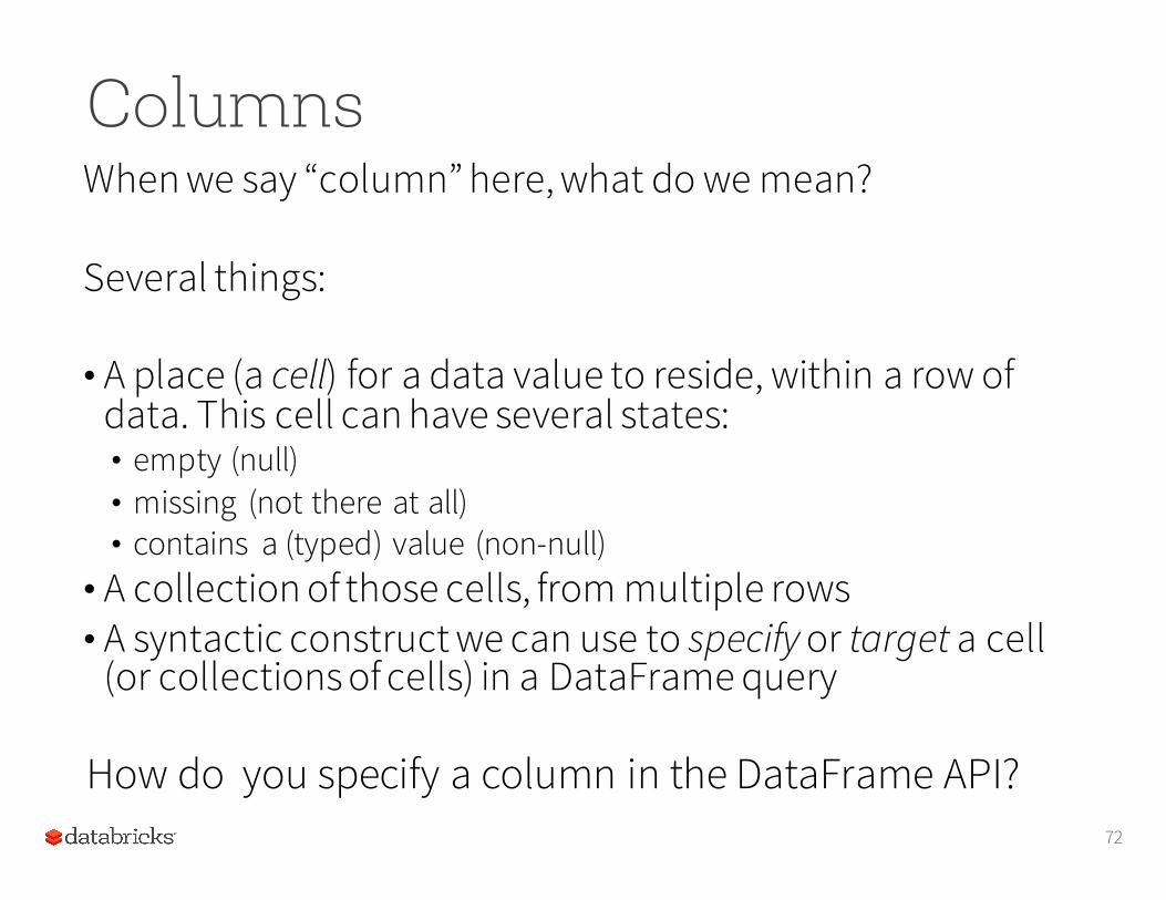
ColumnsWhen we say “column” here, what do we mean?
Several things:
• A place (a cell) for a data value to reside, within a row of data. This cell can have several states:• empty (null)• missing (not there at all)• contains a (typed) value (non-null)
• A collection of those cells, from multiple rows• A syntactic construct we can use to specify or target a cell
(or collections of cells) in a DataFrame query
72
How do you specify a column in the DataFrame API?
Columns
73
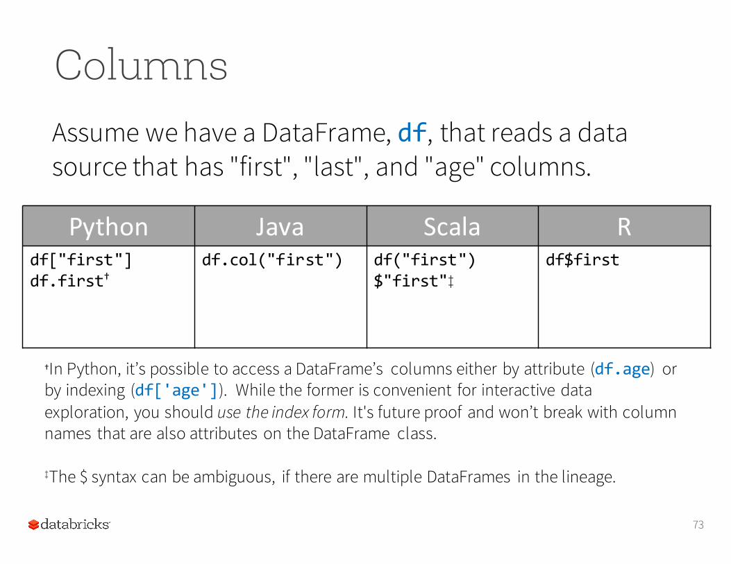
Assume we have a DataFrame, df, that reads a data source that has "first", "last", and "age" columns.
Python Java Scala Rdf["first"]df.first†
df.col("first") df("first")$"first"‡
df$first
†In Python, it’s possible to access a DataFrame’s columns either by attribute (df.age) or by indexing (df['age']). While the former is convenient for interactive data exploration, you should use the index form. It's future proof and won’t break with column names that are also attributes on the DataFrame class.
‡The $ syntax can be ambiguous, if there are multiple DataFrames in the lineage.
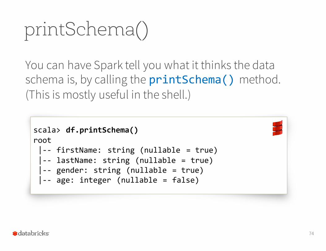
printSchema()
You can have Spark tell you what it thinks the data schema is, by calling the printSchema() method. (This is mostly useful in the shell.)
74
scala> df.printSchema()root|-‐-‐ firstName: string (nullable = true)|-‐-‐ lastName: string (nullable = true)|-‐-‐ gender: string (nullable = true)|-‐-‐ age: integer (nullable = false)
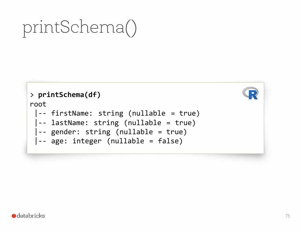
printSchema()
75
> printSchema(df)root|-‐-‐ firstName: string (nullable = true)|-‐-‐ lastName: string (nullable = true)|-‐-‐ gender: string (nullable = true)|-‐-‐ age: integer (nullable = false)
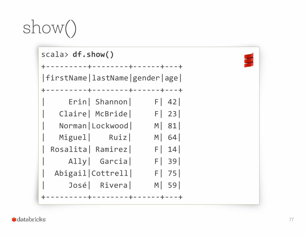
show()You can look at the first n elements in a DataFrame with the show() method. If not specified, n defaults to 20.
This method is an action: It:• reads (or re-reads) the input source• executes the RDD DAG across the cluster•pulls the n elements back to the driver JVM•displays those elements in a tabular form
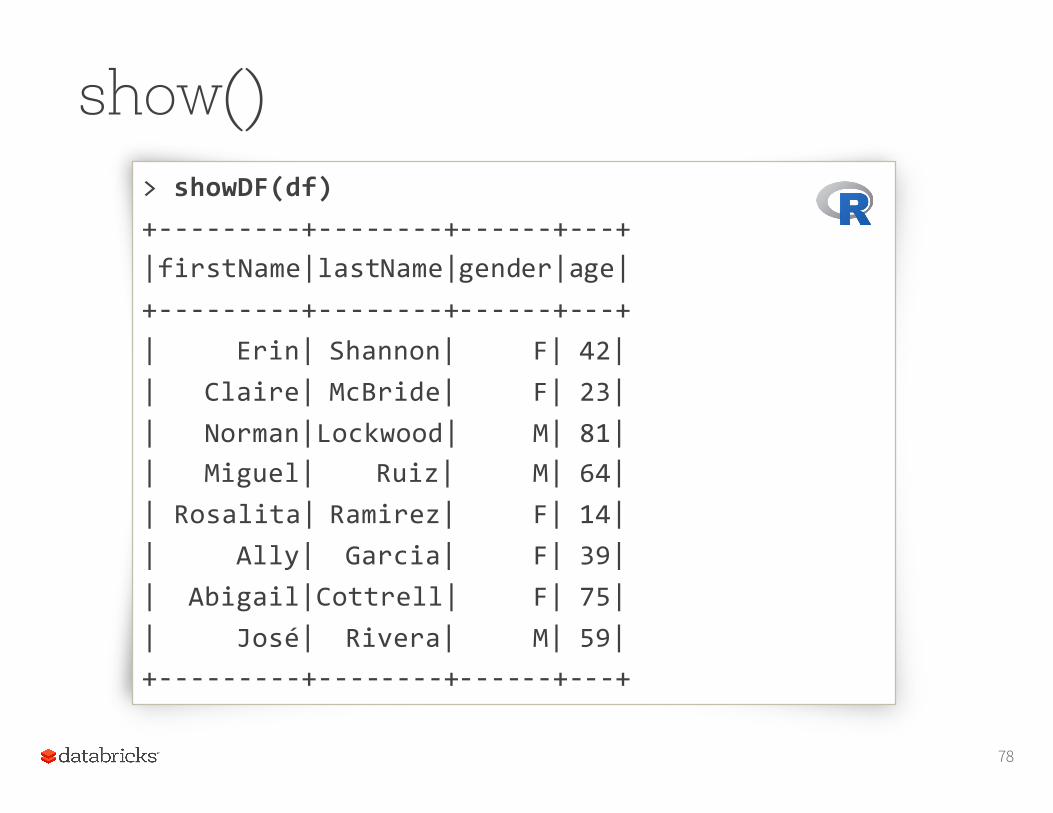
Note: In R, the function is showDF()76
show()
77
scala> df.show()+-‐-‐-‐-‐-‐-‐-‐-‐-‐+-‐-‐-‐-‐-‐-‐-‐-‐+-‐-‐-‐-‐-‐-‐+-‐-‐-‐+|firstName|lastName|gender|age|+-‐-‐-‐-‐-‐-‐-‐-‐-‐+-‐-‐-‐-‐-‐-‐-‐-‐+-‐-‐-‐-‐-‐-‐+-‐-‐-‐+| Erin| Shannon| F| 42|| Claire| McBride| F| 23|| Norman|Lockwood| M| 81|| Miguel| Ruiz| M| 64|| Rosalita| Ramirez| F| 14|| Ally| Garcia| F| 39|| Abigail|Cottrell| F| 75|| José| Rivera| M| 59|+-‐-‐-‐-‐-‐-‐-‐-‐-‐+-‐-‐-‐-‐-‐-‐-‐-‐+-‐-‐-‐-‐-‐-‐+-‐-‐-‐+
show()
78
> showDF(df)+-‐-‐-‐-‐-‐-‐-‐-‐-‐+-‐-‐-‐-‐-‐-‐-‐-‐+-‐-‐-‐-‐-‐-‐+-‐-‐-‐+|firstName|lastName|gender|age|+-‐-‐-‐-‐-‐-‐-‐-‐-‐+-‐-‐-‐-‐-‐-‐-‐-‐+-‐-‐-‐-‐-‐-‐+-‐-‐-‐+| Erin| Shannon| F| 42|| Claire| McBride| F| 23|| Norman|Lockwood| M| 81|| Miguel| Ruiz| M| 64|| Rosalita| Ramirez| F| 14|| Ally| Garcia| F| 39|| Abigail|Cottrell| F| 75|| José| Rivera| M| 59|+-‐-‐-‐-‐-‐-‐-‐-‐-‐+-‐-‐-‐-‐-‐-‐-‐-‐+-‐-‐-‐-‐-‐-‐+-‐-‐-‐+
cache()
•Spark can cache a DataFrame, using an in-memory columnar format, by calling df.cache() (which just calls df.persist(MEMORY_ONLY)). •Spark will scan only those columns used by the
DataFrame and will automatically tune compression to minimize memory usage and GC pressure. • You can call the unpersist() method to remove
the cached data from memory.
79
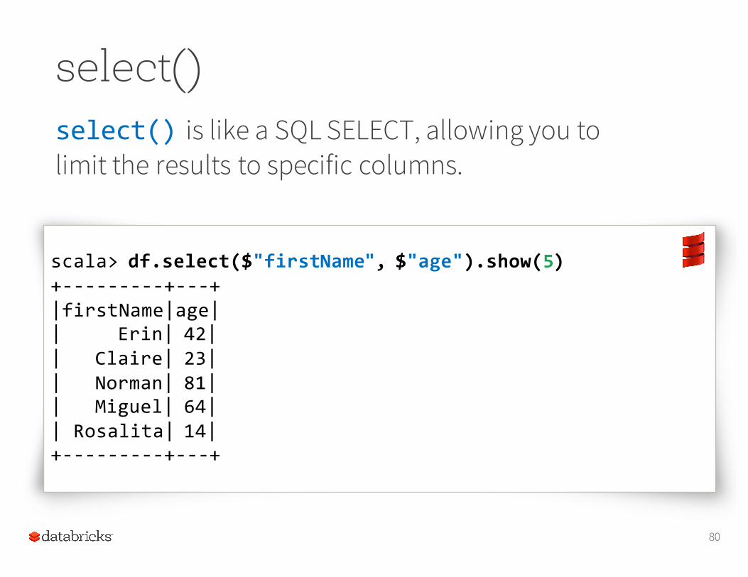
select()select() is like a SQL SELECT, allowing you to limit the results to specific columns.
80
scala> df.select($"firstName", $"age").show(5)+-‐-‐-‐-‐-‐-‐-‐-‐-‐+-‐-‐-‐+|firstName|age|| Erin| 42|| Claire| 23|| Norman| 81|| Miguel| 64|| Rosalita| 14|+-‐-‐-‐-‐-‐-‐-‐-‐-‐+-‐-‐-‐+
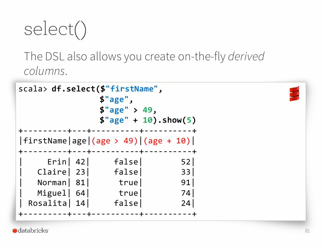
select()The DSL also allows you create on-the-fly derived columns.
81
scala> df.select($"firstName",$"age",$"age" > 49,$"age" + 10).show(5)
+-‐-‐-‐-‐-‐-‐-‐-‐-‐+-‐-‐-‐+-‐-‐-‐-‐-‐-‐-‐-‐-‐-‐+-‐-‐-‐-‐-‐-‐-‐-‐-‐-‐+|firstName|age|(age > 49)|(age + 10)|+-‐-‐-‐-‐-‐-‐-‐-‐-‐+-‐-‐-‐+-‐-‐-‐-‐-‐-‐-‐-‐-‐-‐+-‐-‐-‐-‐-‐-‐-‐-‐-‐-‐+| Erin| 42| false| 52|| Claire| 23| false| 33|| Norman| 81| true| 91|| Miguel| 64| true| 74|| Rosalita| 14| false| 24|+-‐-‐-‐-‐-‐-‐-‐-‐-‐+-‐-‐-‐+-‐-‐-‐-‐-‐-‐-‐-‐-‐-‐+-‐-‐-‐-‐-‐-‐-‐-‐-‐-‐+
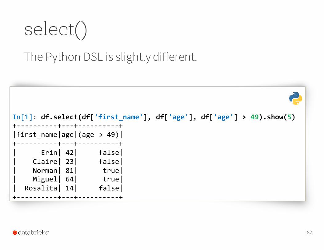
select()The Python DSL is slightly different.
82
In[1]: df.select(df['first_name'], df['age'], df['age'] > 49).show(5)+-‐-‐-‐-‐-‐-‐-‐-‐-‐-‐+-‐-‐-‐+-‐-‐-‐-‐-‐-‐-‐-‐-‐-‐+|first_name|age|(age > 49)|+-‐-‐-‐-‐-‐-‐-‐-‐-‐-‐+-‐-‐-‐+-‐-‐-‐-‐-‐-‐-‐-‐-‐-‐+| Erin| 42| false|| Claire| 23| false|| Norman| 81| true|| Miguel| 64| true|| Rosalita| 14| false|+-‐-‐-‐-‐-‐-‐-‐-‐-‐-‐+-‐-‐-‐+-‐-‐-‐-‐-‐-‐-‐-‐-‐-‐+
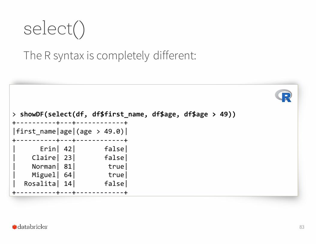
select()The R syntax is completely different:
83
> showDF(select(df, df$first_name, df$age, df$age > 49))+-‐-‐-‐-‐-‐-‐-‐-‐-‐-‐+-‐-‐-‐+-‐-‐-‐-‐-‐-‐-‐-‐-‐-‐-‐-‐+|first_name|age|(age > 49.0)|+-‐-‐-‐-‐-‐-‐-‐-‐-‐-‐+-‐-‐-‐+-‐-‐-‐-‐-‐-‐-‐-‐-‐-‐-‐-‐+| Erin| 42| false|| Claire| 23| false|| Norman| 81| true|| Miguel| 64| true|| Rosalita| 14| false|+-‐-‐-‐-‐-‐-‐-‐-‐-‐-‐+-‐-‐-‐+-‐-‐-‐-‐-‐-‐-‐-‐-‐-‐-‐-‐+
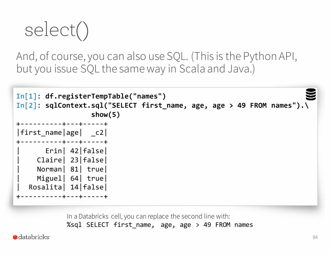
select()And, of course, you can also use SQL. (This is the Python API, but you issue SQL the same way in Scala and Java.)
84
In[1]: df.registerTempTable("names")In[2]: sqlContext.sql("SELECT first_name, age, age > 49 FROM names").\
show(5)+-‐-‐-‐-‐-‐-‐-‐-‐-‐-‐+-‐-‐-‐+-‐-‐-‐-‐-‐+|first_name|age| _c2|+-‐-‐-‐-‐-‐-‐-‐-‐-‐-‐+-‐-‐-‐+-‐-‐-‐-‐-‐+| Erin| 42|false|| Claire| 23|false|| Norman| 81| true|| Miguel| 64| true|| Rosalita| 14|false|+-‐-‐-‐-‐-‐-‐-‐-‐-‐-‐+-‐-‐-‐+-‐-‐-‐-‐-‐+
In a Databricks cell, you can replace the second line with:%sql SELECT first_name, age, age > 49 FROM names
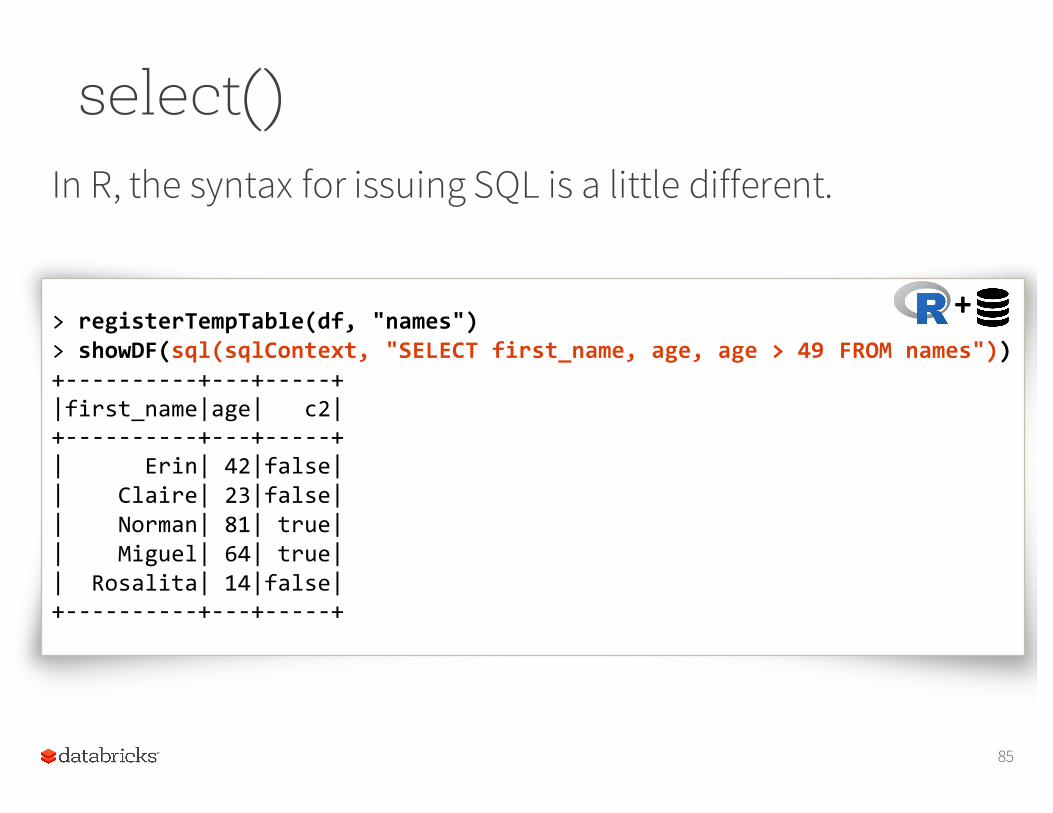
select()In R, the syntax for issuing SQL is a little different.
85
> registerTempTable(df, "names")> showDF(sql(sqlContext, "SELECT first_name, age, age > 49 FROM names"))+-‐-‐-‐-‐-‐-‐-‐-‐-‐-‐+-‐-‐-‐+-‐-‐-‐-‐-‐+|first_name|age| c2|+-‐-‐-‐-‐-‐-‐-‐-‐-‐-‐+-‐-‐-‐+-‐-‐-‐-‐-‐+| Erin| 42|false|| Claire| 23|false|| Norman| 81| true|| Miguel| 64| true|| Rosalita| 14|false|+-‐-‐-‐-‐-‐-‐-‐-‐-‐-‐+-‐-‐-‐+-‐-‐-‐-‐-‐+
+
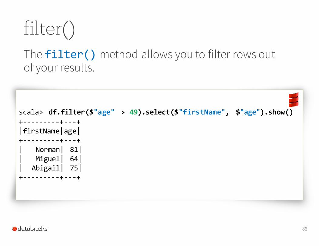
filter()The filter() method allows you to filter rows out of your results.
86
scala> df.filter($"age" > 49).select($"firstName", $"age").show()+-‐-‐-‐-‐-‐-‐-‐-‐-‐+-‐-‐-‐+|firstName|age|+-‐-‐-‐-‐-‐-‐-‐-‐-‐+-‐-‐-‐+| Norman| 81|| Miguel| 64|| Abigail| 75|+-‐-‐-‐-‐-‐-‐-‐-‐-‐+-‐-‐-‐+
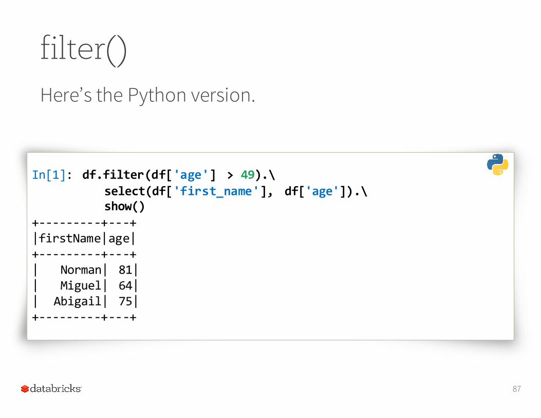
filter()Here’s the Python version.
87
In[1]: df.filter(df['age'] > 49).\select(df['first_name'], df['age']).\show()
+-‐-‐-‐-‐-‐-‐-‐-‐-‐+-‐-‐-‐+|firstName|age|+-‐-‐-‐-‐-‐-‐-‐-‐-‐+-‐-‐-‐+| Norman| 81|| Miguel| 64|| Abigail| 75|+-‐-‐-‐-‐-‐-‐-‐-‐-‐+-‐-‐-‐+
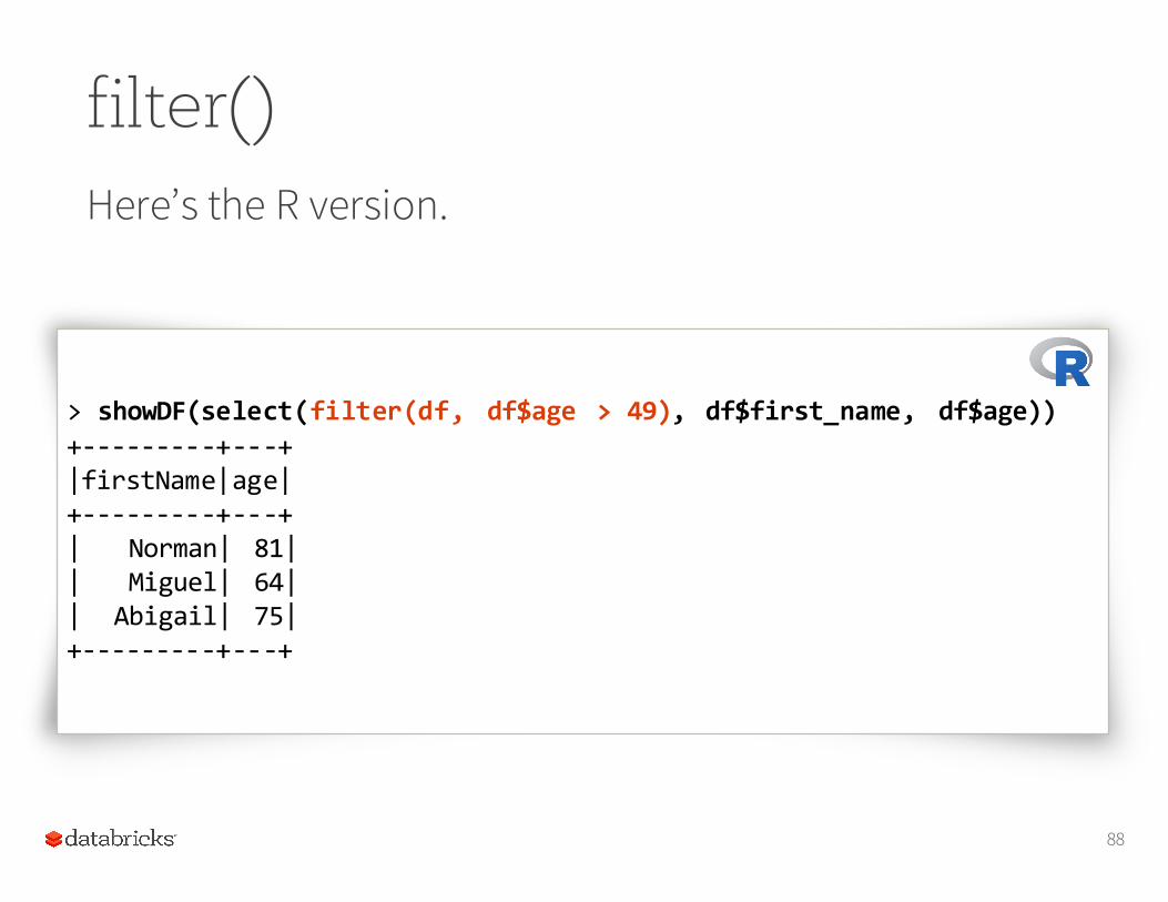
filter()Here’s the R version.
88
> showDF(select(filter(df, df$age > 49), df$first_name, df$age))+-‐-‐-‐-‐-‐-‐-‐-‐-‐+-‐-‐-‐+|firstName|age|+-‐-‐-‐-‐-‐-‐-‐-‐-‐+-‐-‐-‐+| Norman| 81|| Miguel| 64|| Abigail| 75|+-‐-‐-‐-‐-‐-‐-‐-‐-‐+-‐-‐-‐+
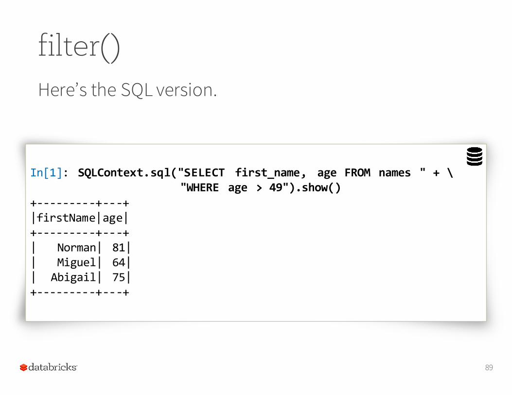
filter()Here’s the SQL version.
89
In[1]: SQLContext.sql("SELECT first_name, age FROM names " + \"WHERE age > 49").show()
+-‐-‐-‐-‐-‐-‐-‐-‐-‐+-‐-‐-‐+|firstName|age|+-‐-‐-‐-‐-‐-‐-‐-‐-‐+-‐-‐-‐+| Norman| 81|| Miguel| 64|| Abigail| 75|+-‐-‐-‐-‐-‐-‐-‐-‐-‐+-‐-‐-‐+
Hands On
Open the hands on notebook again. Let's take a look at the second section, entitled select and filter(and a couple more).
90
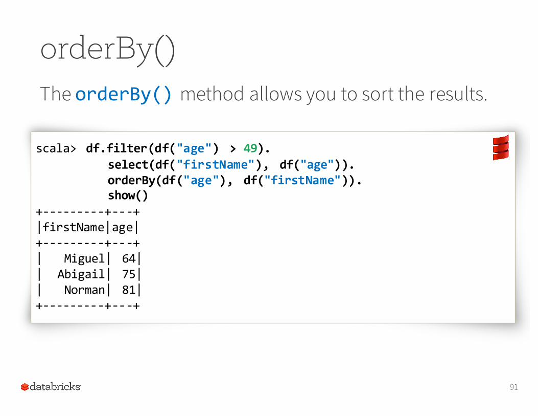
orderBy()The orderBy() method allows you to sort the results.
91
scala> df.filter(df("age") > 49).select(df("firstName"), df("age")).orderBy(df("age"), df("firstName")).show()
+-‐-‐-‐-‐-‐-‐-‐-‐-‐+-‐-‐-‐+|firstName|age|+-‐-‐-‐-‐-‐-‐-‐-‐-‐+-‐-‐-‐+| Miguel| 64|| Abigail| 75|| Norman| 81|+-‐-‐-‐-‐-‐-‐-‐-‐-‐+-‐-‐-‐+
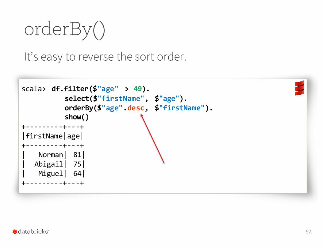
orderBy()It’s easy to reverse the sort order.
92
scala> df.filter($"age" > 49).select($"firstName", $"age").orderBy($"age".desc, $"firstName").show()
+-‐-‐-‐-‐-‐-‐-‐-‐-‐+-‐-‐-‐+|firstName|age|+-‐-‐-‐-‐-‐-‐-‐-‐-‐+-‐-‐-‐+| Norman| 81|| Abigail| 75|| Miguel| 64|+-‐-‐-‐-‐-‐-‐-‐-‐-‐+-‐-‐-‐+
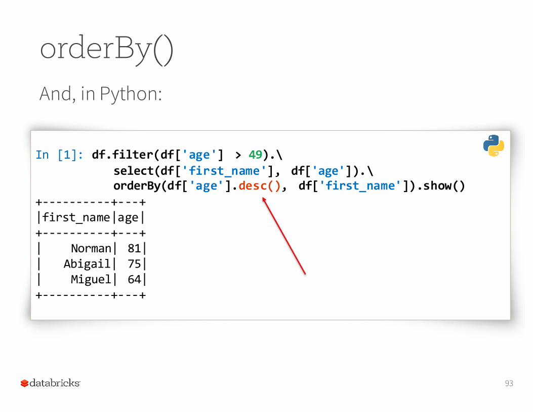
orderBy()And, in Python:
93
In [1]: df.filter(df['age'] > 49).\select(df['first_name'], df['age']).\orderBy(df['age'].desc(), df['first_name']).show()
+-‐-‐-‐-‐-‐-‐-‐-‐-‐-‐+-‐-‐-‐+|first_name|age|+-‐-‐-‐-‐-‐-‐-‐-‐-‐-‐+-‐-‐-‐+| Norman| 81|| Abigail| 75|| Miguel| 64|+-‐-‐-‐-‐-‐-‐-‐-‐-‐-‐+-‐-‐-‐+
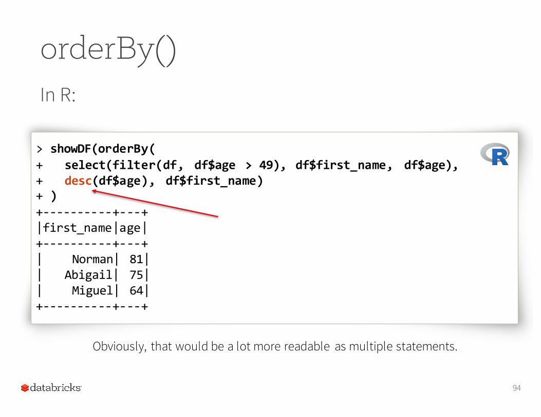
orderBy()In R:
94
> showDF(orderBy(+ select(filter(df, df$age > 49), df$first_name, df$age),+ desc(df$age), df$first_name)+ )+-‐-‐-‐-‐-‐-‐-‐-‐-‐-‐+-‐-‐-‐+|first_name|age|+-‐-‐-‐-‐-‐-‐-‐-‐-‐-‐+-‐-‐-‐+| Norman| 81|| Abigail| 75|| Miguel| 64|+-‐-‐-‐-‐-‐-‐-‐-‐-‐-‐+-‐-‐-‐+
Obviously, that would be a lot more readable as multiple statements.
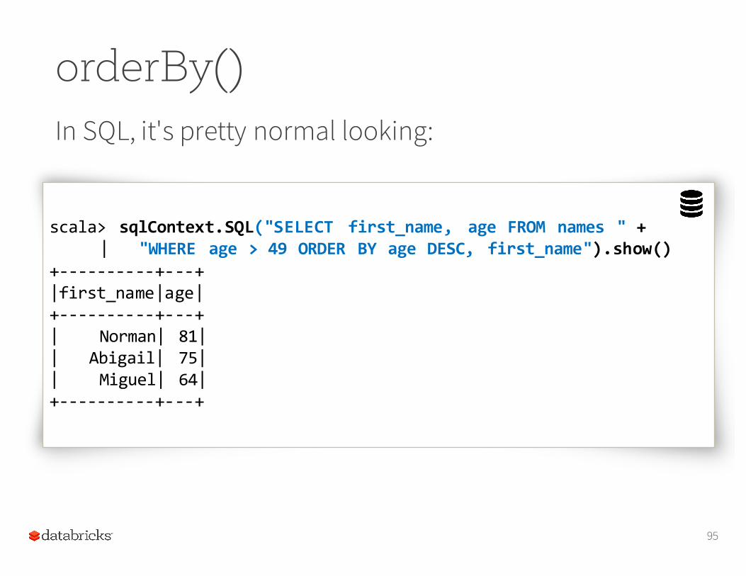
orderBy()In SQL, it's pretty normal looking:
95
scala> sqlContext.SQL("SELECT first_name, age FROM names " +| "WHERE age > 49 ORDER BY age DESC, first_name").show()
+-‐-‐-‐-‐-‐-‐-‐-‐-‐-‐+-‐-‐-‐+|first_name|age|+-‐-‐-‐-‐-‐-‐-‐-‐-‐-‐+-‐-‐-‐+| Norman| 81|| Abigail| 75|| Miguel| 64|+-‐-‐-‐-‐-‐-‐-‐-‐-‐-‐+-‐-‐-‐+
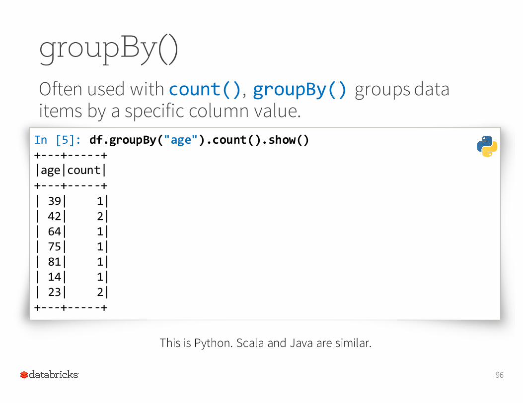
groupBy()Often used with count(), groupBy() groups data items by a specific column value.
96
In [5]: df.groupBy("age").count().show()+-‐-‐-‐+-‐-‐-‐-‐-‐+|age|count|+-‐-‐-‐+-‐-‐-‐-‐-‐+| 39| 1|| 42| 2|| 64| 1|| 75| 1|| 81| 1|| 14| 1|| 23| 2|+-‐-‐-‐+-‐-‐-‐-‐-‐+
This is Python. Scala and Java are similar.
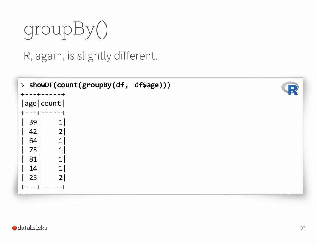
groupBy()R, again, is slightly different.
97
> showDF(count(groupBy(df, df$age)))+-‐-‐-‐+-‐-‐-‐-‐-‐+|age|count|+-‐-‐-‐+-‐-‐-‐-‐-‐+| 39| 1|| 42| 2|| 64| 1|| 75| 1|| 81| 1|| 14| 1|| 23| 2|+-‐-‐-‐+-‐-‐-‐-‐-‐+
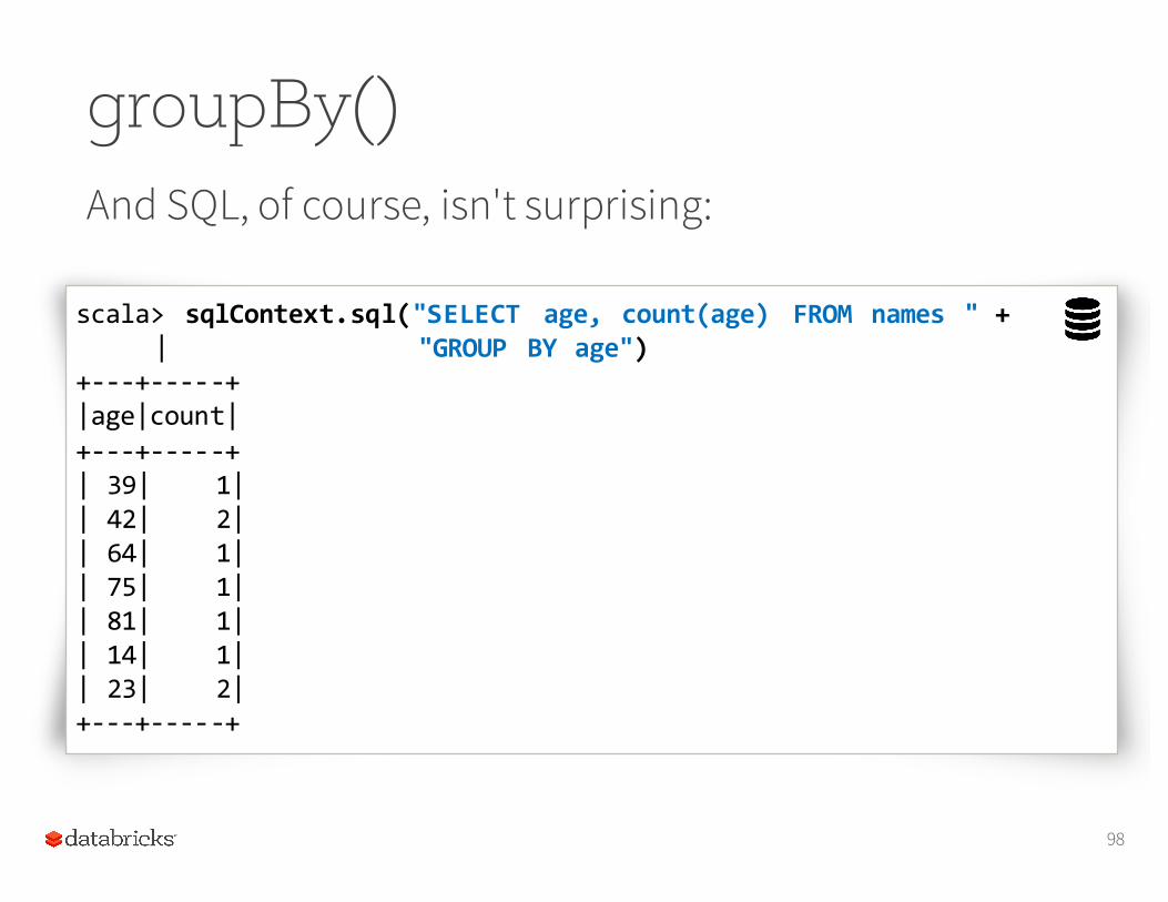
groupBy()And SQL, of course, isn't surprising:
98
scala> sqlContext.sql("SELECT age, count(age) FROM names " +| "GROUP BY age")
+-‐-‐-‐+-‐-‐-‐-‐-‐+|age|count|+-‐-‐-‐+-‐-‐-‐-‐-‐+| 39| 1|| 42| 2|| 64| 1|| 75| 1|| 81| 1|| 14| 1|| 23| 2|+-‐-‐-‐+-‐-‐-‐-‐-‐+
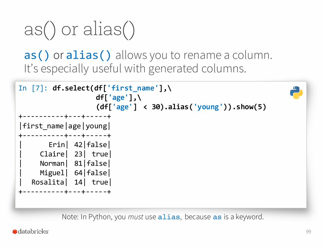
as() or alias()as() or alias() allows you to rename a column. It’s especially useful with generated columns.
99
In [7]: df.select(df['first_name'],\df['age'],\(df['age'] < 30).alias('young')).show(5)
+-‐-‐-‐-‐-‐-‐-‐-‐-‐-‐+-‐-‐-‐+-‐-‐-‐-‐-‐+|first_name|age|young|+-‐-‐-‐-‐-‐-‐-‐-‐-‐-‐+-‐-‐-‐+-‐-‐-‐-‐-‐+| Erin| 42|false|| Claire| 23| true|| Norman| 81|false|| Miguel| 64|false|| Rosalita| 14| true|+-‐-‐-‐-‐-‐-‐-‐-‐-‐-‐+-‐-‐-‐+-‐-‐-‐-‐-‐+
Note: In Python, you must use alias, because as is a keyword.
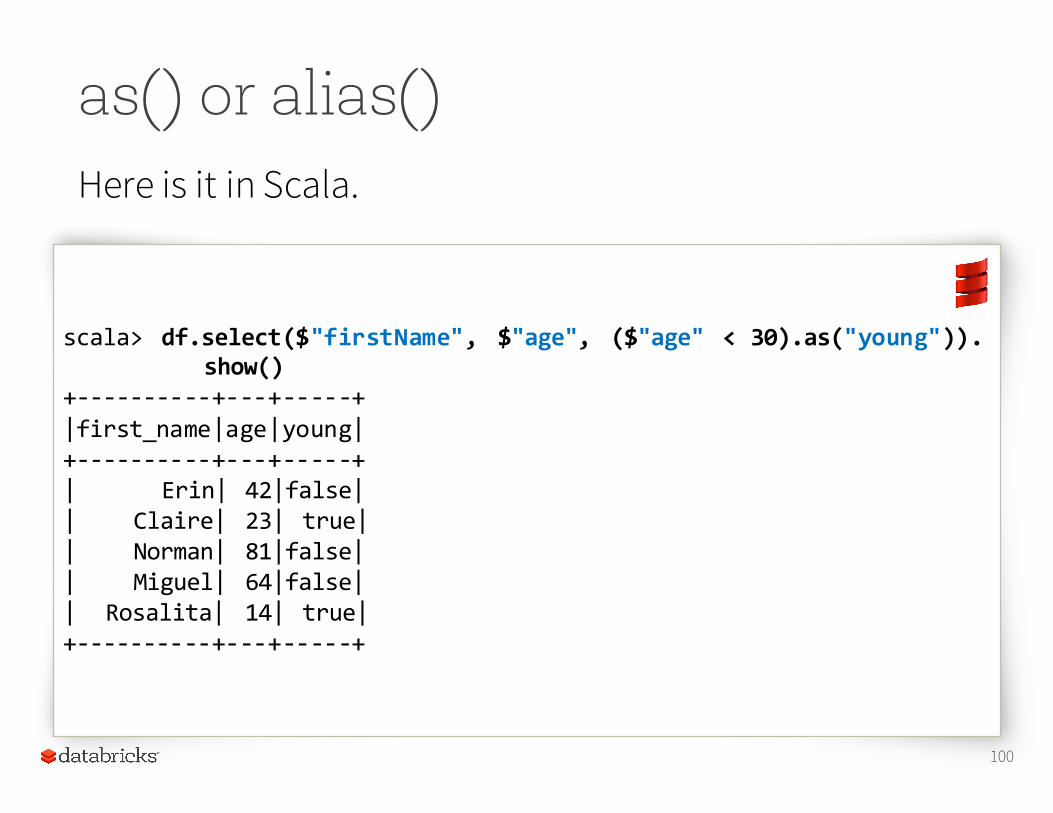
as() or alias()Here is it in Scala.
100
scala> df.select($"firstName", $"age", ($"age" < 30).as("young")).show()
+-‐-‐-‐-‐-‐-‐-‐-‐-‐-‐+-‐-‐-‐+-‐-‐-‐-‐-‐+|first_name|age|young|+-‐-‐-‐-‐-‐-‐-‐-‐-‐-‐+-‐-‐-‐+-‐-‐-‐-‐-‐+| Erin| 42|false|| Claire| 23| true|| Norman| 81|false|| Miguel| 64|false|| Rosalita| 14| true|+-‐-‐-‐-‐-‐-‐-‐-‐-‐-‐+-‐-‐-‐+-‐-‐-‐-‐-‐+
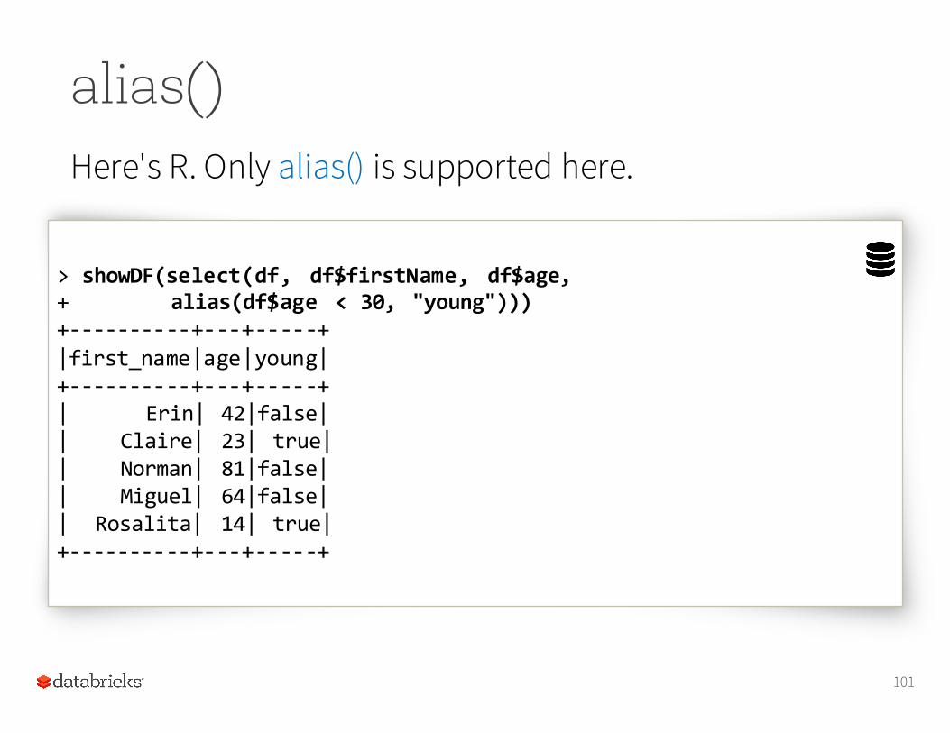
alias()Here's R. Only alias() is supported here.
101
> showDF(select(df, df$firstName, df$age, + alias(df$age < 30, "young")))+-‐-‐-‐-‐-‐-‐-‐-‐-‐-‐+-‐-‐-‐+-‐-‐-‐-‐-‐+|first_name|age|young|+-‐-‐-‐-‐-‐-‐-‐-‐-‐-‐+-‐-‐-‐+-‐-‐-‐-‐-‐+| Erin| 42|false|| Claire| 23| true|| Norman| 81|false|| Miguel| 64|false|| Rosalita| 14| true|+-‐-‐-‐-‐-‐-‐-‐-‐-‐-‐+-‐-‐-‐+-‐-‐-‐-‐-‐+
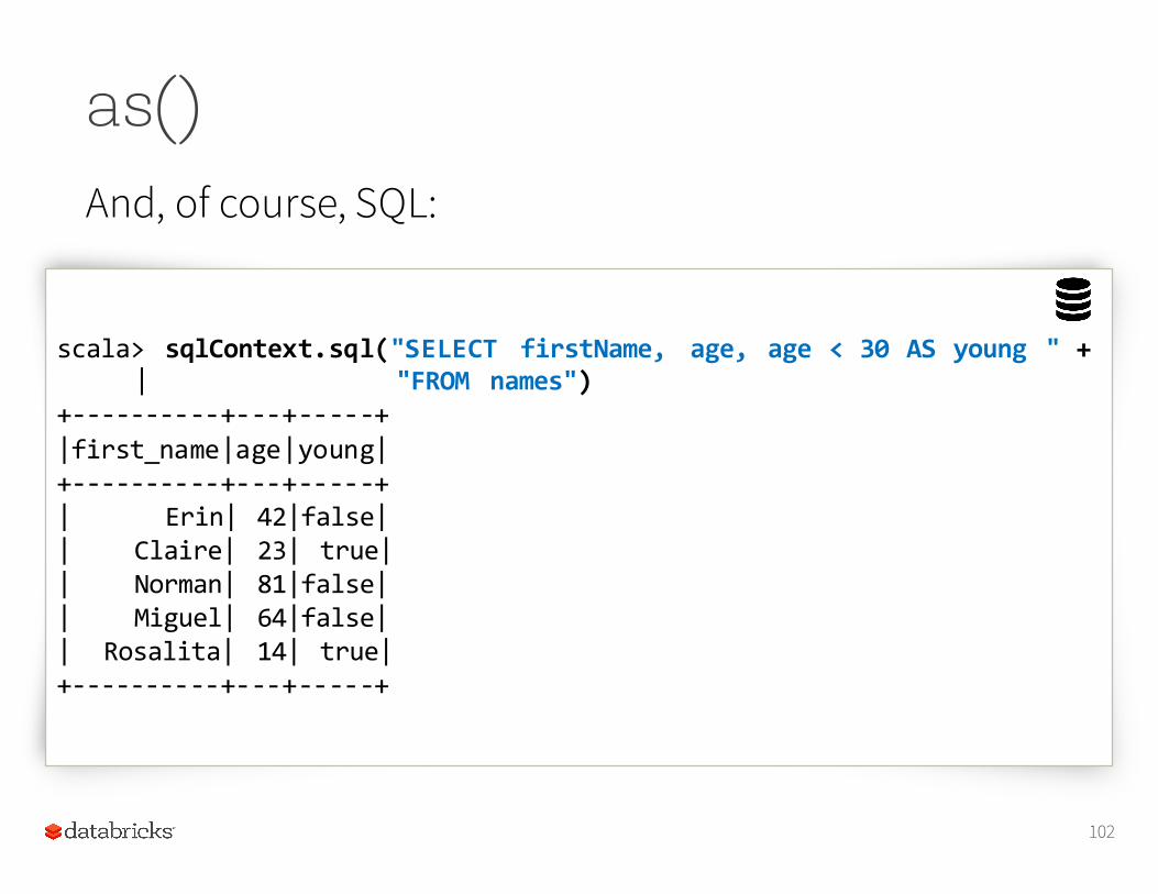
as()And, of course, SQL:
102
scala> sqlContext.sql("SELECT firstName, age, age < 30 AS young " +| "FROM names")
+-‐-‐-‐-‐-‐-‐-‐-‐-‐-‐+-‐-‐-‐+-‐-‐-‐-‐-‐+|first_name|age|young|+-‐-‐-‐-‐-‐-‐-‐-‐-‐-‐+-‐-‐-‐+-‐-‐-‐-‐-‐+| Erin| 42|false|| Claire| 23| true|| Norman| 81|false|| Miguel| 64|false|| Rosalita| 14| true|+-‐-‐-‐-‐-‐-‐-‐-‐-‐-‐+-‐-‐-‐+-‐-‐-‐-‐-‐+
Hands On
Switch back to your hands on notebook, and look at the section entitled orderBy, groupBy and alias.
103
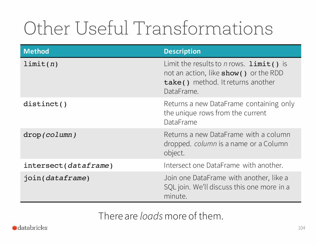
Method Description
limit(n) Limit the results to n rows. limit() is not an action, like show() or the RDD take() method. It returns another DataFrame.
distinct() Returns a new DataFrame containing only the unique rows from the current DataFrame
drop(column) Returns a new DataFrame with a column dropped. column is a name or a Column object.
intersect(dataframe) Intersect one DataFrame with another.
join(dataframe) Join one DataFrame with another, like a SQL join. We’ll discuss this one more in a minute.
104
Other Useful Transformations
There are loads more of them.
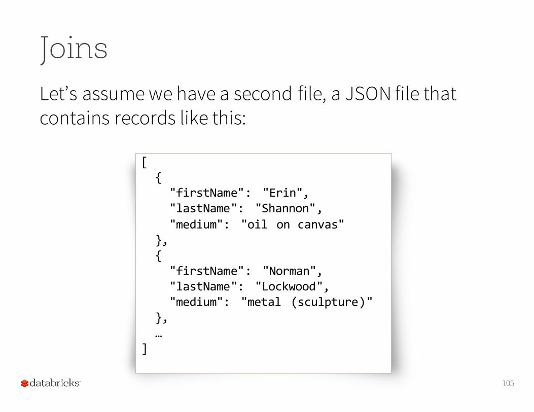
JoinsLet’s assume we have a second file, a JSON file that contains records like this:
105
[{
"firstName": "Erin","lastName": "Shannon","medium": "oil on canvas"
},{
"firstName": "Norman","lastName": "Lockwood","medium": "metal (sculpture)"
},…
]
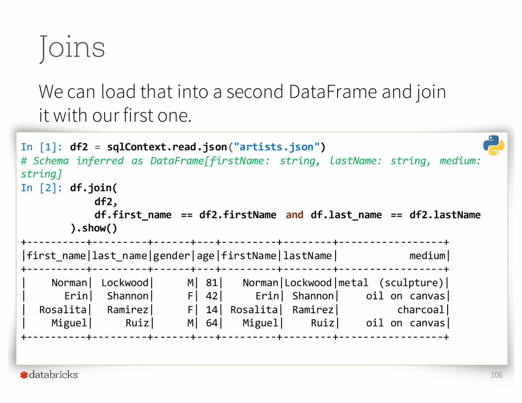
JoinsWe can load that into a second DataFrame and join it with our first one.
106
In [1]: df2 = sqlContext.read.json("artists.json")# Schema inferred as DataFrame[firstName: string, lastName: string, medium: string]In [2]: df.join(
df2, df.first_name == df2.firstName and df.last_name == df2.lastName
).show()+-‐-‐-‐-‐-‐-‐-‐-‐-‐-‐+-‐-‐-‐-‐-‐-‐-‐-‐-‐+-‐-‐-‐-‐-‐-‐+-‐-‐-‐+-‐-‐-‐-‐-‐-‐-‐-‐-‐+-‐-‐-‐-‐-‐-‐-‐-‐+-‐-‐-‐-‐-‐-‐-‐-‐-‐-‐-‐-‐-‐-‐-‐-‐-‐+|first_name|last_name|gender|age|firstName|lastName| medium|+-‐-‐-‐-‐-‐-‐-‐-‐-‐-‐+-‐-‐-‐-‐-‐-‐-‐-‐-‐+-‐-‐-‐-‐-‐-‐+-‐-‐-‐+-‐-‐-‐-‐-‐-‐-‐-‐-‐+-‐-‐-‐-‐-‐-‐-‐-‐+-‐-‐-‐-‐-‐-‐-‐-‐-‐-‐-‐-‐-‐-‐-‐-‐-‐+| Norman| Lockwood| M| 81| Norman|Lockwood|metal (sculpture)|| Erin| Shannon| F| 42| Erin| Shannon| oil on canvas|| Rosalita| Ramirez| F| 14| Rosalita| Ramirez| charcoal|| Miguel| Ruiz| M| 64| Miguel| Ruiz| oil on canvas|+-‐-‐-‐-‐-‐-‐-‐-‐-‐-‐+-‐-‐-‐-‐-‐-‐-‐-‐-‐+-‐-‐-‐-‐-‐-‐+-‐-‐-‐+-‐-‐-‐-‐-‐-‐-‐-‐-‐+-‐-‐-‐-‐-‐-‐-‐-‐+-‐-‐-‐-‐-‐-‐-‐-‐-‐-‐-‐-‐-‐-‐-‐-‐-‐+
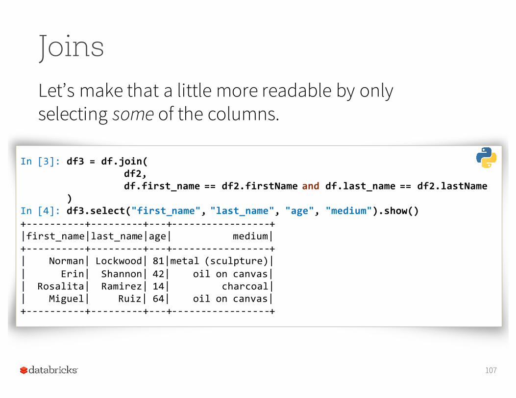
JoinsLet’s make that a little more readable by only selecting some of the columns.
107
In [3]: df3 = df.join(df2, df.first_name == df2.firstName and df.last_name == df2.lastName
)In [4]: df3.select("first_name", "last_name", "age", "medium").show()+-‐-‐-‐-‐-‐-‐-‐-‐-‐-‐+-‐-‐-‐-‐-‐-‐-‐-‐-‐+-‐-‐-‐+-‐-‐-‐-‐-‐-‐-‐-‐-‐-‐-‐-‐-‐-‐-‐-‐-‐+|first_name|last_name|age| medium|+-‐-‐-‐-‐-‐-‐-‐-‐-‐-‐+-‐-‐-‐-‐-‐-‐-‐-‐-‐+-‐-‐-‐+-‐-‐-‐-‐-‐-‐-‐-‐-‐-‐-‐-‐-‐-‐-‐-‐-‐+| Norman| Lockwood| 81|metal (sculpture)|| Erin| Shannon| 42| oil on canvas|| Rosalita| Ramirez| 14| charcoal|| Miguel| Ruiz| 64| oil on canvas|+-‐-‐-‐-‐-‐-‐-‐-‐-‐-‐+-‐-‐-‐-‐-‐-‐-‐-‐-‐+-‐-‐-‐+-‐-‐-‐-‐-‐-‐-‐-‐-‐-‐-‐-‐-‐-‐-‐-‐-‐+
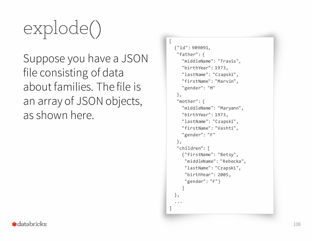
explode()[{"id": 909091,"father": {"middleName": "Travis","birthYear": 1973,"lastName": "Czapski","firstName": "Marvin","gender": "M"
},"mother": {"middleName": "Maryann","birthYear": 1973,"lastName": "Czapski","firstName": "Vashti","gender": "F"
},"children": [{"firstName": "Betsy","middleName": "Rebecka","lastName": "Czapski","birthYear": 2005, "gender": "F"}
]},...
]
108
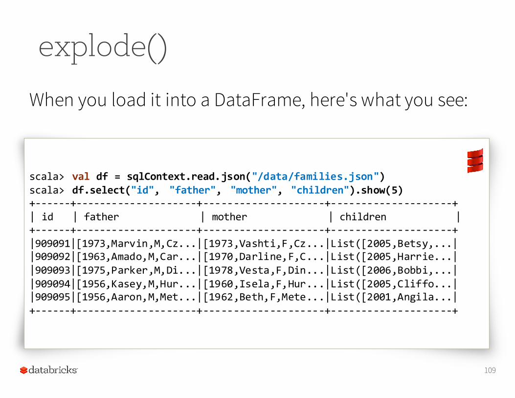
Suppose you have a JSON file consisting of data about families. The file is an array of JSON objects, as shown here.
explode()
When you load it into a DataFrame, here's what you see:
109
scala> val df = sqlContext.read.json("/data/families.json")scala> df.select("id", "father", "mother", "children").show(5)+-‐-‐-‐-‐-‐-‐+-‐-‐-‐-‐-‐-‐-‐-‐-‐-‐-‐-‐-‐-‐-‐-‐-‐-‐-‐-‐+-‐-‐-‐-‐-‐-‐-‐-‐-‐-‐-‐-‐-‐-‐-‐-‐-‐-‐-‐-‐+-‐-‐-‐-‐-‐-‐-‐-‐-‐-‐-‐-‐-‐-‐-‐-‐-‐-‐-‐-‐+| id | father | mother | children | +-‐-‐-‐-‐-‐-‐+-‐-‐-‐-‐-‐-‐-‐-‐-‐-‐-‐-‐-‐-‐-‐-‐-‐-‐-‐-‐+-‐-‐-‐-‐-‐-‐-‐-‐-‐-‐-‐-‐-‐-‐-‐-‐-‐-‐-‐-‐+-‐-‐-‐-‐-‐-‐-‐-‐-‐-‐-‐-‐-‐-‐-‐-‐-‐-‐-‐-‐+ |909091|[1973,Marvin,M,Cz...|[1973,Vashti,F,Cz...|List([2005,Betsy,...| |909092|[1963,Amado,M,Car...|[1970,Darline,F,C...|List([2005,Harrie...| |909093|[1975,Parker,M,Di...|[1978,Vesta,F,Din...|List([2006,Bobbi,...| |909094|[1956,Kasey,M,Hur...|[1960,Isela,F,Hur...|List([2005,Cliffo...| |909095|[1956,Aaron,M,Met...|[1962,Beth,F,Mete...|List([2001,Angila...|+-‐-‐-‐-‐-‐-‐+-‐-‐-‐-‐-‐-‐-‐-‐-‐-‐-‐-‐-‐-‐-‐-‐-‐-‐-‐-‐+-‐-‐-‐-‐-‐-‐-‐-‐-‐-‐-‐-‐-‐-‐-‐-‐-‐-‐-‐-‐+-‐-‐-‐-‐-‐-‐-‐-‐-‐-‐-‐-‐-‐-‐-‐-‐-‐-‐-‐-‐+
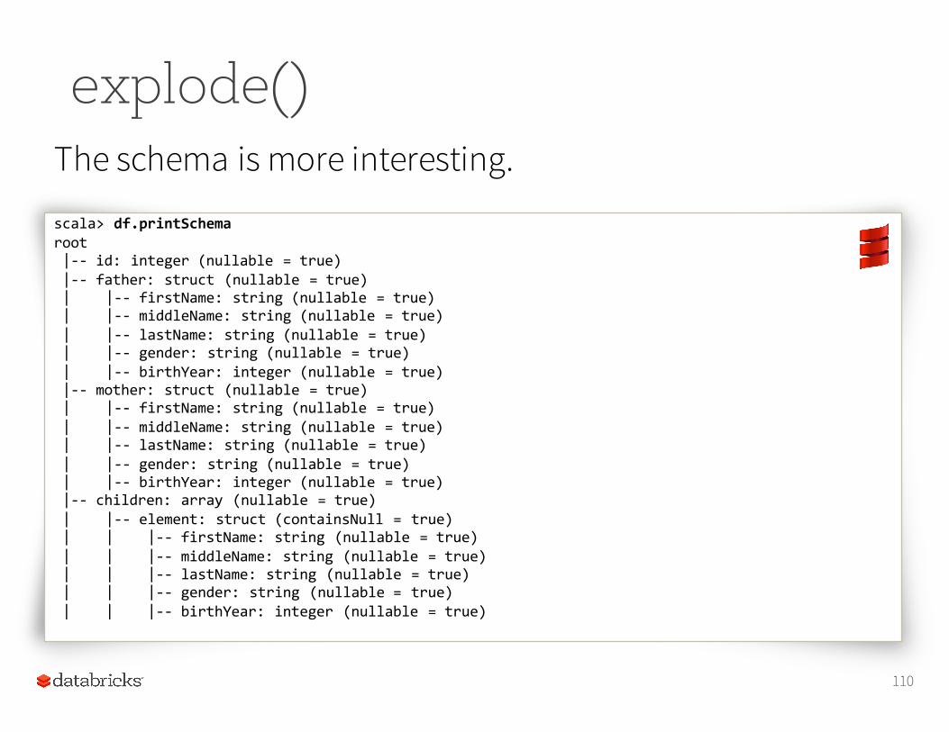
explode()The schema is more interesting.
110
scala> df.printSchemaroot|-‐-‐ id: integer (nullable = true)|-‐-‐ father: struct (nullable = true)| |-‐-‐ firstName: string (nullable = true)| |-‐-‐ middleName: string (nullable = true)| |-‐-‐ lastName: string (nullable = true)| |-‐-‐ gender: string (nullable = true)| |-‐-‐ birthYear: integer (nullable = true)|-‐-‐ mother: struct (nullable = true)| |-‐-‐ firstName: string (nullable = true)| |-‐-‐ middleName: string (nullable = true)| |-‐-‐ lastName: string (nullable = true)| |-‐-‐ gender: string (nullable = true)| |-‐-‐ birthYear: integer (nullable = true)|-‐-‐ children: array (nullable = true)| |-‐-‐ element: struct (containsNull = true)| | |-‐-‐ firstName: string (nullable = true)| | |-‐-‐ middleName: string (nullable = true)| | |-‐-‐ lastName: string (nullable = true)| | |-‐-‐ gender: string (nullable = true)| | |-‐-‐ birthYear: integer (nullable = true)
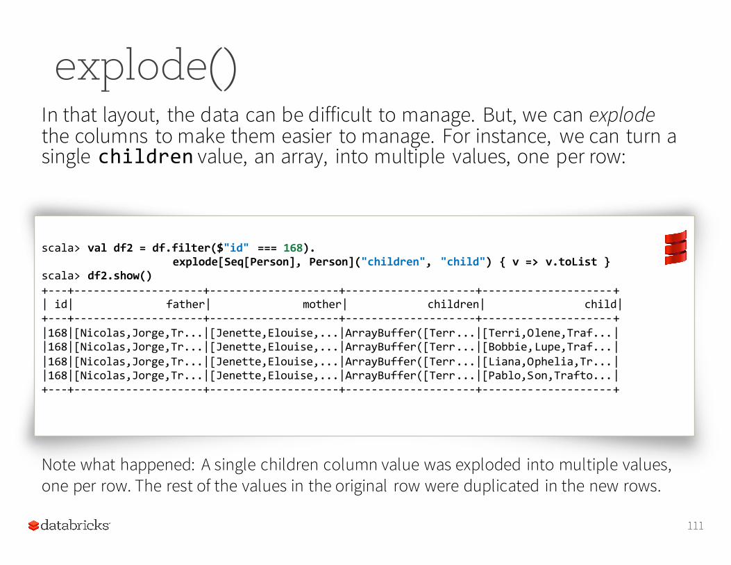
explode()In that layout, the data can be difficult to manage. But, we can explodethe columns to make them easier to manage. For instance, we can turn a single children value, an array, into multiple values, one per row:
111
scala> val df2 = df.filter($"id" === 168).explode[Seq[Person], Person]("children", "child") { v => v.toList }
scala> df2.show() +-‐-‐-‐+-‐-‐-‐-‐-‐-‐-‐-‐-‐-‐-‐-‐-‐-‐-‐-‐-‐-‐-‐-‐+-‐-‐-‐-‐-‐-‐-‐-‐-‐-‐-‐-‐-‐-‐-‐-‐-‐-‐-‐-‐+-‐-‐-‐-‐-‐-‐-‐-‐-‐-‐-‐-‐-‐-‐-‐-‐-‐-‐-‐-‐+-‐-‐-‐-‐-‐-‐-‐-‐-‐-‐-‐-‐-‐-‐-‐-‐-‐-‐-‐-‐+| id| father| mother| children| child|+-‐-‐-‐+-‐-‐-‐-‐-‐-‐-‐-‐-‐-‐-‐-‐-‐-‐-‐-‐-‐-‐-‐-‐+-‐-‐-‐-‐-‐-‐-‐-‐-‐-‐-‐-‐-‐-‐-‐-‐-‐-‐-‐-‐+-‐-‐-‐-‐-‐-‐-‐-‐-‐-‐-‐-‐-‐-‐-‐-‐-‐-‐-‐-‐+-‐-‐-‐-‐-‐-‐-‐-‐-‐-‐-‐-‐-‐-‐-‐-‐-‐-‐-‐-‐+|168|[Nicolas,Jorge,Tr...|[Jenette,Elouise,...|ArrayBuffer([Terr...|[Terri,Olene,Traf...||168|[Nicolas,Jorge,Tr...|[Jenette,Elouise,...|ArrayBuffer([Terr...|[Bobbie,Lupe,Traf...||168|[Nicolas,Jorge,Tr...|[Jenette,Elouise,...|ArrayBuffer([Terr...|[Liana,Ophelia,Tr...||168|[Nicolas,Jorge,Tr...|[Jenette,Elouise,...|ArrayBuffer([Terr...|[Pablo,Son,Trafto...|+-‐-‐-‐+-‐-‐-‐-‐-‐-‐-‐-‐-‐-‐-‐-‐-‐-‐-‐-‐-‐-‐-‐-‐+-‐-‐-‐-‐-‐-‐-‐-‐-‐-‐-‐-‐-‐-‐-‐-‐-‐-‐-‐-‐+-‐-‐-‐-‐-‐-‐-‐-‐-‐-‐-‐-‐-‐-‐-‐-‐-‐-‐-‐-‐+-‐-‐-‐-‐-‐-‐-‐-‐-‐-‐-‐-‐-‐-‐-‐-‐-‐-‐-‐-‐+
Note what happened: A single children column value was exploded into multiple values, one per row. The rest of the values in the original row were duplicated in the new rows.
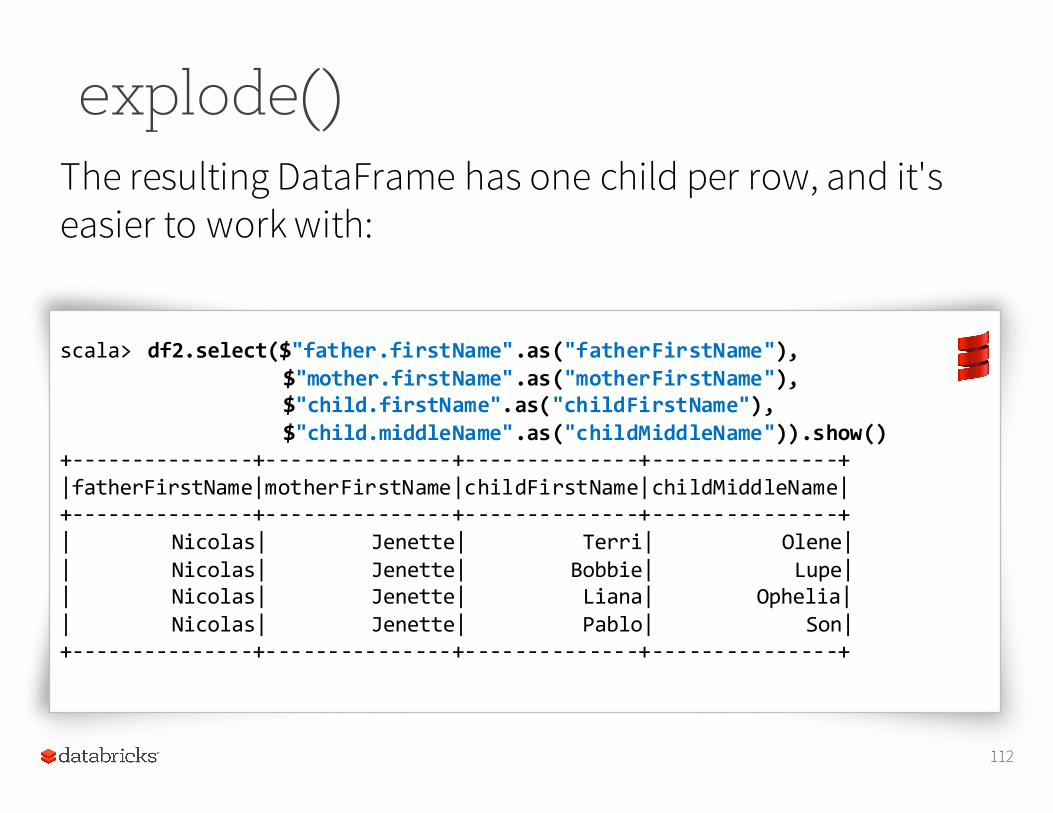
explode()The resulting DataFrame has one child per row, and it's easier to work with:
112
scala> df2.select($"father.firstName".as("fatherFirstName"),$"mother.firstName".as("motherFirstName"),$"child.firstName".as("childFirstName"),$"child.middleName".as("childMiddleName")).show()
+-‐-‐-‐-‐-‐-‐-‐-‐-‐-‐-‐-‐-‐-‐-‐+-‐-‐-‐-‐-‐-‐-‐-‐-‐-‐-‐-‐-‐-‐-‐+-‐-‐-‐-‐-‐-‐-‐-‐-‐-‐-‐-‐-‐-‐+-‐-‐-‐-‐-‐-‐-‐-‐-‐-‐-‐-‐-‐-‐-‐+|fatherFirstName|motherFirstName|childFirstName|childMiddleName|+-‐-‐-‐-‐-‐-‐-‐-‐-‐-‐-‐-‐-‐-‐-‐+-‐-‐-‐-‐-‐-‐-‐-‐-‐-‐-‐-‐-‐-‐-‐+-‐-‐-‐-‐-‐-‐-‐-‐-‐-‐-‐-‐-‐-‐+-‐-‐-‐-‐-‐-‐-‐-‐-‐-‐-‐-‐-‐-‐-‐+| Nicolas| Jenette| Terri| Olene|| Nicolas| Jenette| Bobbie| Lupe|| Nicolas| Jenette| Liana| Ophelia|| Nicolas| Jenette| Pablo| Son|+-‐-‐-‐-‐-‐-‐-‐-‐-‐-‐-‐-‐-‐-‐-‐+-‐-‐-‐-‐-‐-‐-‐-‐-‐-‐-‐-‐-‐-‐-‐+-‐-‐-‐-‐-‐-‐-‐-‐-‐-‐-‐-‐-‐-‐+-‐-‐-‐-‐-‐-‐-‐-‐-‐-‐-‐-‐-‐-‐-‐+
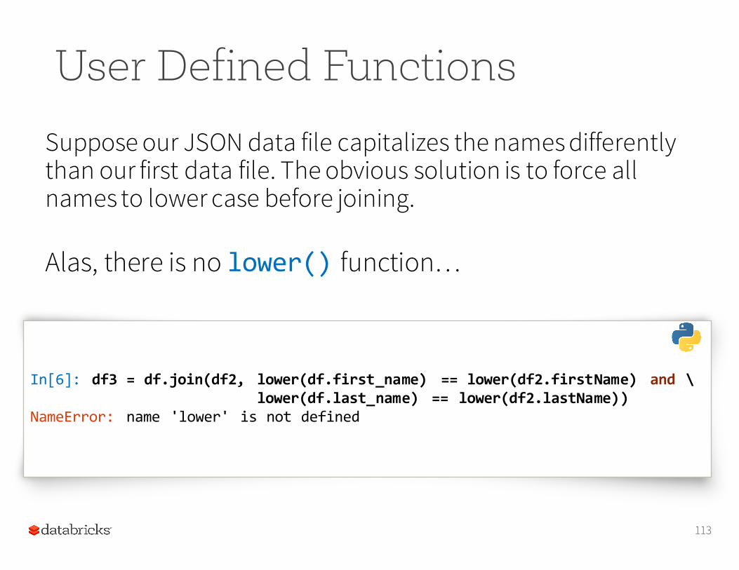
User Defined FunctionsSuppose our JSON data file capitalizes the names differently than our first data file. The obvious solution is to force all names to lower case before joining.
113
In[6]: df3 = df.join(df2, lower(df.first_name) == lower(df2.firstName) and \lower(df.last_name) == lower(df2.lastName))
NameError: name 'lower' is not defined
Alas, there is no lower() function…
User Defined Functions
114
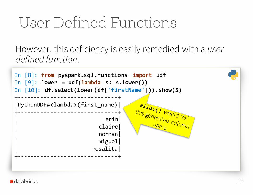
In [8]: from pyspark.sql.functions import udfIn [9]: lower = udf(lambda s: s.lower())In [10]: df.select(lower(df['firstName'])).show(5)+-‐-‐-‐-‐-‐-‐-‐-‐-‐-‐-‐-‐-‐-‐-‐-‐-‐-‐-‐-‐-‐-‐-‐-‐-‐-‐-‐-‐-‐-‐+|PythonUDF#<lambda>(first_name)|+-‐-‐-‐-‐-‐-‐-‐-‐-‐-‐-‐-‐-‐-‐-‐-‐-‐-‐-‐-‐-‐-‐-‐-‐-‐-‐-‐-‐-‐-‐+| erin|| claire|| norman|| miguel|| rosalita|+-‐-‐-‐-‐-‐-‐-‐-‐-‐-‐-‐-‐-‐-‐-‐-‐-‐-‐-‐-‐-‐-‐-‐-‐-‐-‐-‐-‐-‐-‐+
However, this deficiency is easily remedied with a user defined function.
User Defined Functions
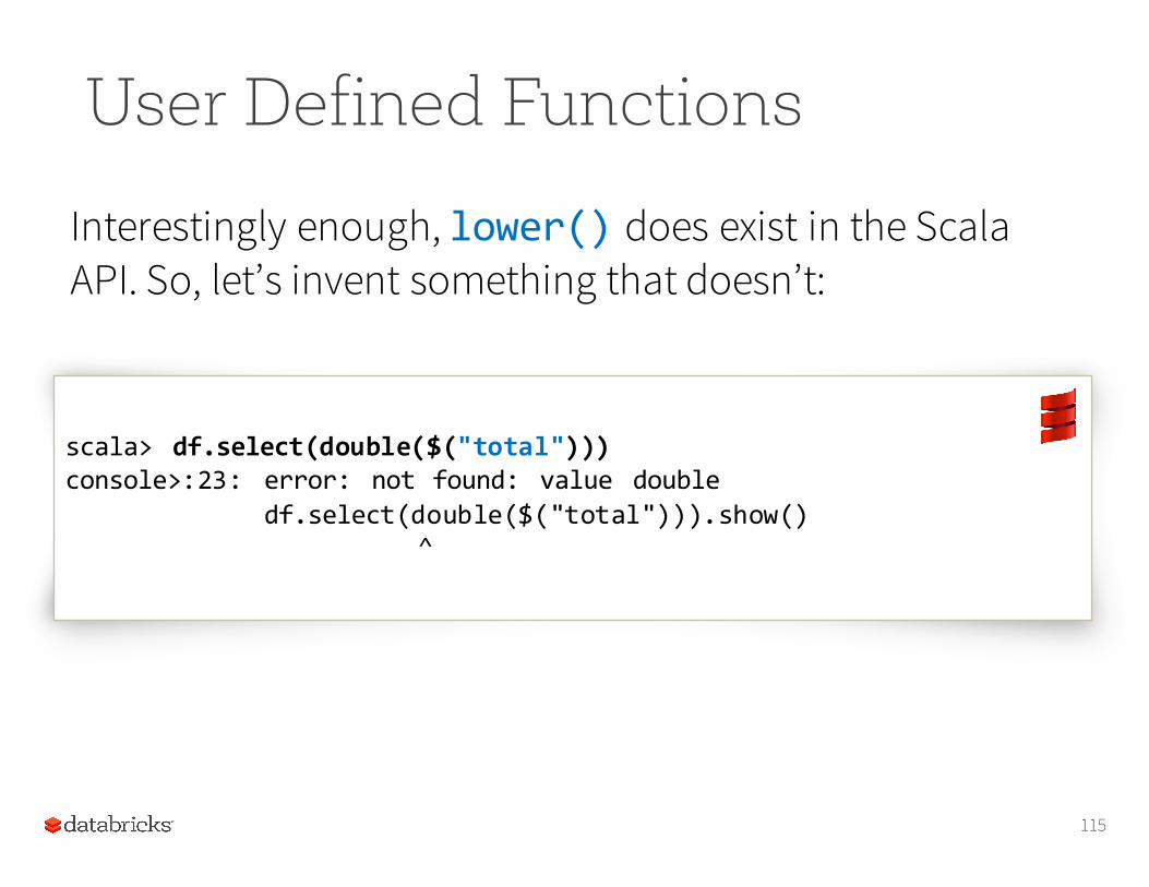
Interestingly enough, lower() does exist in the Scala API. So, let’s invent something that doesn’t:
115
scala> df.select(double($("total")))console>:23: error: not found: value double
df.select(double($("total"))).show()^
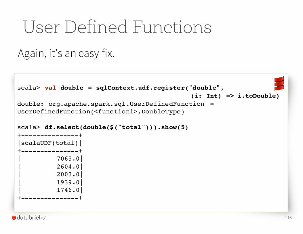
User Defined FunctionsAgain, it’s an easy fix.
116
scala> val double = sqlContext.udf.register("double",(i: Int) => i.toDouble)
double: org.apache.spark.sql.UserDefinedFunction = UserDefinedFunction(<function1>,DoubleType)
scala> df.select(double($("total"))).show(5)+---------------+|scalaUDF(total)|+---------------+| 7065.0|| 2604.0|| 2003.0|| 1939.0|| 1746.0|+---------------+
User Defined Functions
UDFs are not currently supported in R.
117
Lab
In Databricks, you'll find a DataFrames lab.
•Choose the Scala lab or the Python lab.•Copy the appropriate lab into your Databricks
folder.•Open the notebook and follow the instructions. At
the bottom of the lab, you'll find an assignment to be completed.
118
Writing DataFrames
• You can write DataFrames out, as well. When doing ETL, this is a very common requirement.• In most cases, if you can read a data format, you can
write that data format, as well.• If you're writing to a text file format (e.g., JSON), you'll
typically get multiple output files.
119
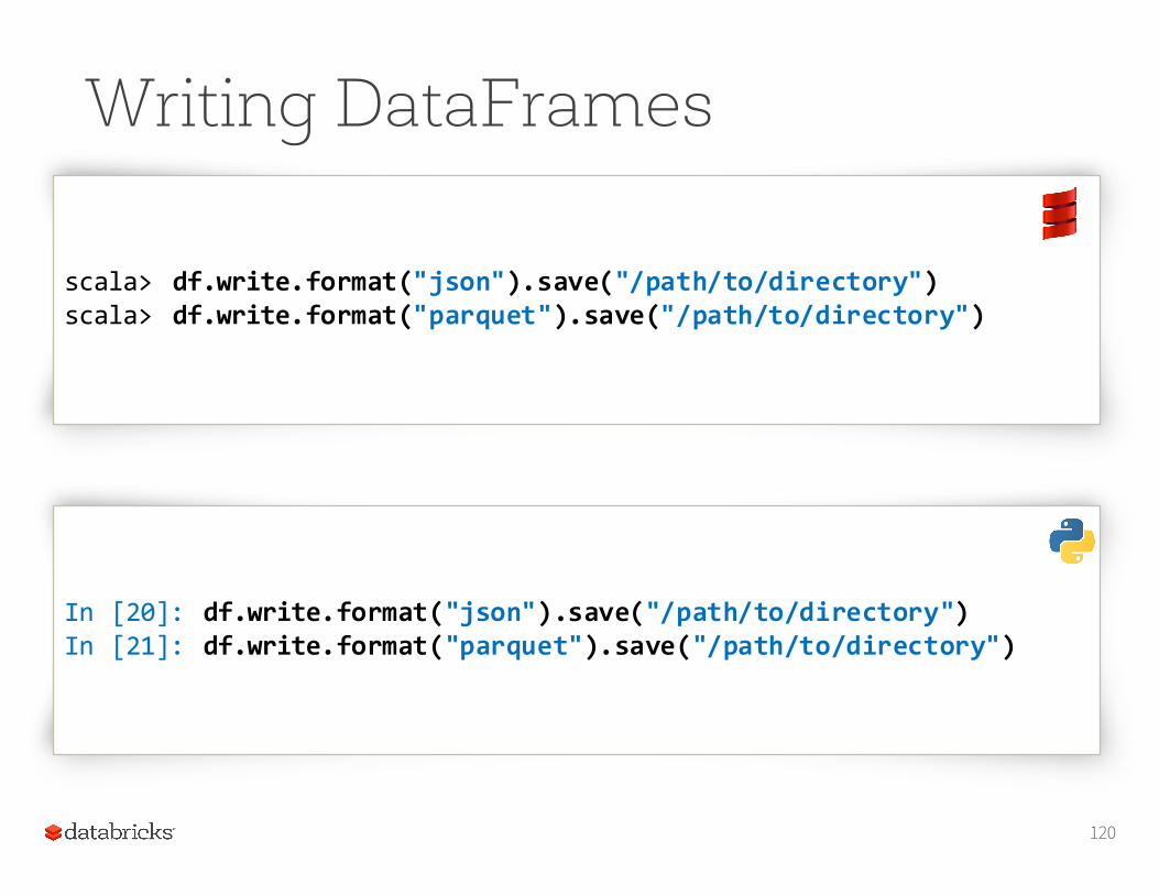
Writing DataFrames
120
scala> df.write.format("json").save("/path/to/directory")scala> df.write.format("parquet").save("/path/to/directory")
In [20]: df.write.format("json").save("/path/to/directory")In [21]: df.write.format("parquet").save("/path/to/directory")
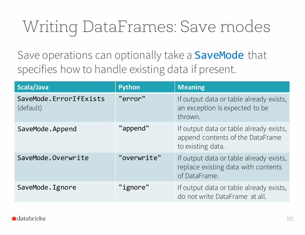
Writing DataFrames: Save modesSave operations can optionally take a SaveMode that specifies how to handle existing data if present.
121
Scala/Java Python MeaningSaveMode.ErrorIfExists(default)
"error" If output data or table already exists, an exception is expected to be thrown.
SaveMode.Append "append" If output data or table already exists, append contents of the DataFrame to existing data.
SaveMode.Overwrite "overwrite" If output data or table already exists, replace existing data with contents of DataFrame.
SaveMode.Ignore "ignore" If output data or table already exists, do not write DataFrame at all.
Writing DataFrames: Save modes
Warning: These save modes do not utilize any locking and are not atomic.
122
Thus, it is not safe to have multiple writers attempting to write to the same location. Additionally, when performing a overwrite, the data will be deleted before writing out the new data.
Writing DataFrames: Hive•When working with a HiveContext, you can save
a DataFrame as a persistent table, with the saveAsTable() method. •Unlike registerTempTable(),saveAsTable() materializes the DataFrame (i.e., runs the DAG) and creates a pointer to the data in the Hive metastore. •Persistent tables will exist even after your Spark
program has restarted.
123
Writing Data Frames: Hive
•By default, saveAsTable() will create a managed table: the metastore controls the location of the data. Data in a managed table is also deleted automatically when the table is dropped.
124
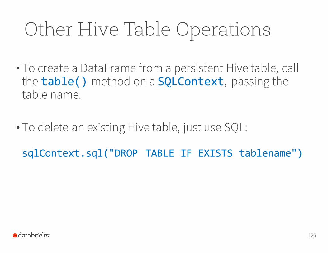
Other Hive Table Operations
•To create a DataFrame from a persistent Hive table, call the table() method on a SQLContext, passing the table name.
•To delete an existing Hive table, just use SQL:
sqlContext.sql("DROP TABLE IF EXISTS tablename")
125
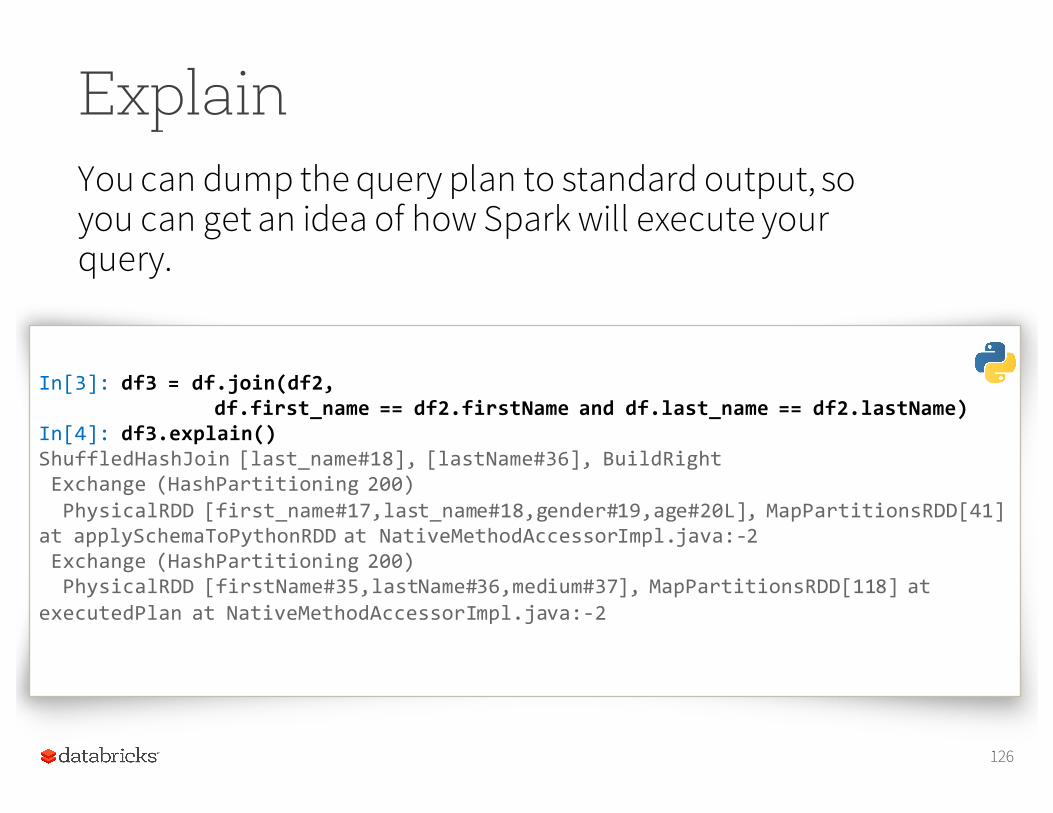
ExplainYou can dump the query plan to standard output, so you can get an idea of how Spark will execute your query.
126
In[3]: df3 = df.join(df2, df.first_name == df2.firstName and df.last_name == df2.lastName)
In[4]: df3.explain()ShuffledHashJoin [last_name#18], [lastName#36], BuildRightExchange (HashPartitioning 200)PhysicalRDD [first_name#17,last_name#18,gender#19,age#20L], MapPartitionsRDD[41]
at applySchemaToPythonRDD at NativeMethodAccessorImpl.java:-‐2Exchange (HashPartitioning 200)PhysicalRDD [firstName#35,lastName#36,medium#37], MapPartitionsRDD[118] at
executedPlan at NativeMethodAccessorImpl.java:-‐2
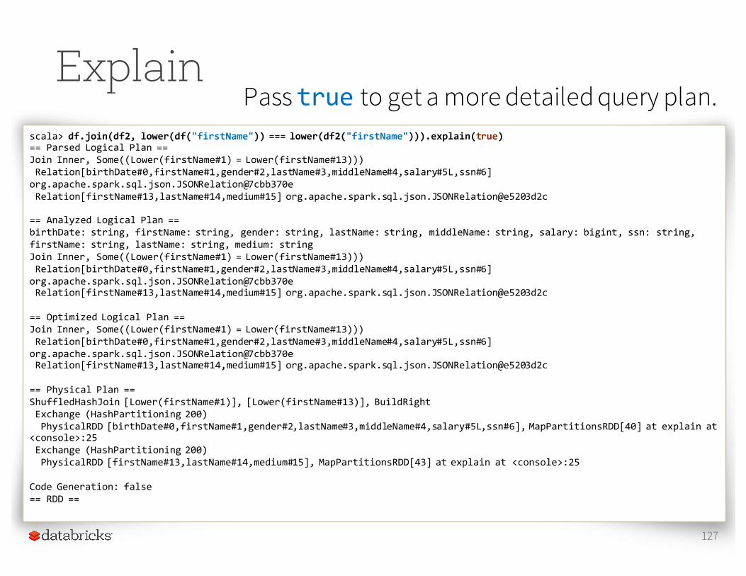
ExplainPass true to get a more detailed query plan.
127
scala> df.join(df2, lower(df("firstName")) === lower(df2("firstName"))).explain(true)== Parsed Logical Plan ==Join Inner, Some((Lower(firstName#1) = Lower(firstName#13)))Relation[birthDate#0,firstName#1,gender#2,lastName#3,middleName#4,salary#5L,ssn#6] org.apache.spark.sql.json.JSONRelation@7cbb370eRelation[firstName#13,lastName#14,medium#15] org.apache.spark.sql.json.JSONRelation@e5203d2c
== Analyzed Logical Plan ==birthDate: string, firstName: string, gender: string, lastName: string, middleName: string, salary: bigint, ssn: string, firstName: string, lastName: string, medium: stringJoin Inner, Some((Lower(firstName#1) = Lower(firstName#13)))Relation[birthDate#0,firstName#1,gender#2,lastName#3,middleName#4,salary#5L,ssn#6] org.apache.spark.sql.json.JSONRelation@7cbb370eRelation[firstName#13,lastName#14,medium#15] org.apache.spark.sql.json.JSONRelation@e5203d2c
== Optimized Logical Plan ==Join Inner, Some((Lower(firstName#1) = Lower(firstName#13)))Relation[birthDate#0,firstName#1,gender#2,lastName#3,middleName#4,salary#5L,ssn#6] org.apache.spark.sql.json.JSONRelation@7cbb370eRelation[firstName#13,lastName#14,medium#15] org.apache.spark.sql.json.JSONRelation@e5203d2c
== Physical Plan ==ShuffledHashJoin [Lower(firstName#1)], [Lower(firstName#13)], BuildRightExchange (HashPartitioning 200)PhysicalRDD [birthDate#0,firstName#1,gender#2,lastName#3,middleName#4,salary#5L,ssn#6], MapPartitionsRDD[40] at explain at
<console>:25Exchange (HashPartitioning 200)PhysicalRDD [firstName#13,lastName#14,medium#15], MapPartitionsRDD[43] at explain at <console>:25
Code Generation: false== RDD ==
Spark SQL: Just a little more info
Recall that Spark SQL operations generally return DataFrames. This means you can freely mix DataFrames and SQL.
128
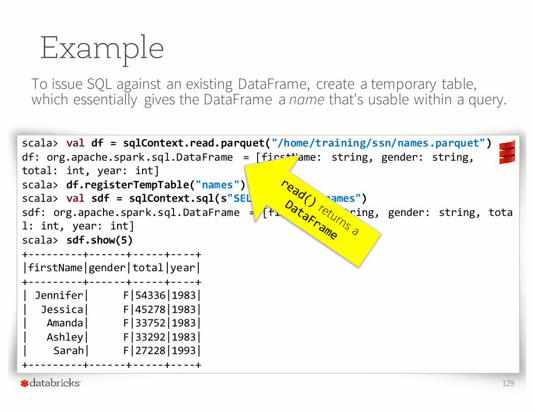
ExampleTo issue SQL against an existing DataFrame, create a temporary table, which essentially gives the DataFrame a name that's usable within a query.
129
scala> val df = sqlContext.read.parquet("/home/training/ssn/names.parquet")df: org.apache.spark.sql.DataFrame = [firstName: string, gender: string, total: int, year: int]scala> df.registerTempTable("names")scala> val sdf = sqlContext.sql(s"SELECT * FROM names")sdf: org.apache.spark.sql.DataFrame = [firstName: string, gender: string, total: int, year: int] scala> sdf.show(5)+-‐-‐-‐-‐-‐-‐-‐-‐-‐+-‐-‐-‐-‐-‐-‐+-‐-‐-‐-‐-‐+-‐-‐-‐-‐+|firstName|gender|total|year| +-‐-‐-‐-‐-‐-‐-‐-‐-‐+-‐-‐-‐-‐-‐-‐+-‐-‐-‐-‐-‐+-‐-‐-‐-‐+ | Jennifer| F|54336|1983|| Jessica| F|45278|1983|| Amanda| F|33752|1983|| Ashley| F|33292|1983|| Sarah| F|27228|1993|+-‐-‐-‐-‐-‐-‐-‐-‐-‐+-‐-‐-‐-‐-‐-‐+-‐-‐-‐-‐-‐+-‐-‐-‐-‐+
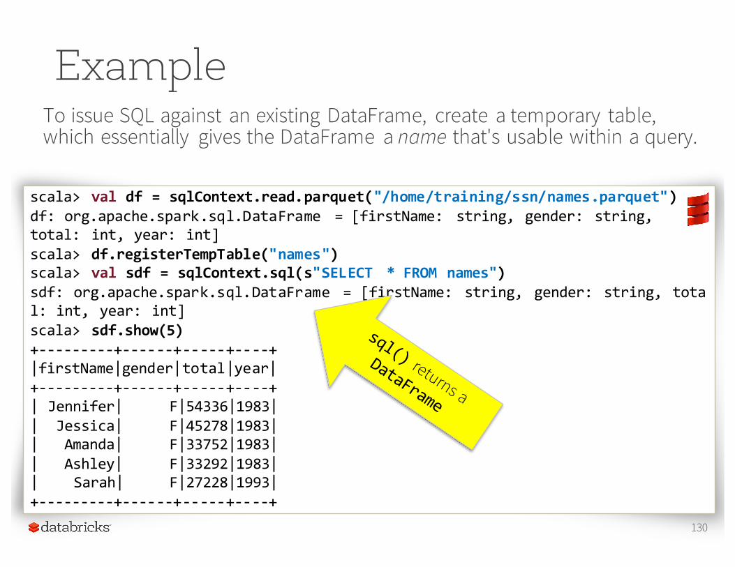
ExampleTo issue SQL against an existing DataFrame, create a temporary table, which essentially gives the DataFrame a name that's usable within a query.
130
scala> val df = sqlContext.read.parquet("/home/training/ssn/names.parquet")df: org.apache.spark.sql.DataFrame = [firstName: string, gender: string, total: int, year: int]scala> df.registerTempTable("names")scala> val sdf = sqlContext.sql(s"SELECT * FROM names")sdf: org.apache.spark.sql.DataFrame = [firstName: string, gender: string, total: int, year: int] scala> sdf.show(5)+-‐-‐-‐-‐-‐-‐-‐-‐-‐+-‐-‐-‐-‐-‐-‐+-‐-‐-‐-‐-‐+-‐-‐-‐-‐+|firstName|gender|total|year| +-‐-‐-‐-‐-‐-‐-‐-‐-‐+-‐-‐-‐-‐-‐-‐+-‐-‐-‐-‐-‐+-‐-‐-‐-‐+ | Jennifer| F|54336|1983|| Jessica| F|45278|1983|| Amanda| F|33752|1983|| Ashley| F|33292|1983|| Sarah| F|27228|1993|+-‐-‐-‐-‐-‐-‐-‐-‐-‐+-‐-‐-‐-‐-‐-‐+-‐-‐-‐-‐-‐+-‐-‐-‐-‐+
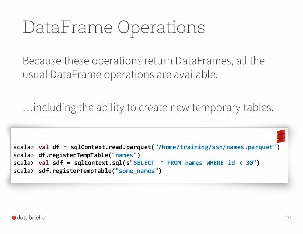
Because these operations return DataFrames, all the usual DataFrame operations are available.
…including the ability to create new temporary tables.
131
DataFrame Operations
scala> val df = sqlContext.read.parquet("/home/training/ssn/names.parquet")scala> df.registerTempTable("names")scala> val sdf = sqlContext.sql(s"SELECT * FROM names WHERE id < 30")scala> sdf.registerTempTable("some_names")
SQL and RDDs
•Because SQL queries return DataFrames, and DataFrames are built on RDDs, you can use normal RDD operations on the results of a SQL query.•However, as with any DataFrame, it's best to stick
with DataFrame operations.
132
133
DataFrame Advanced Tips
• It is possible to coalesce or repartition DataFrames
•Catalyst does not do any automatic determination of partitions. After a shuffle, The DataFrame API uses spark.sql.shuffle.partititions to determine the number of partitions.
Machine Learning Integration
Spark 1.2 introduced a new package called spark.ml, which aims to provide a uniform set of high-level APIs that help users create and tune practical machine learning pipelines.
Spark ML standardizes APIs for machine learning algorithms to make it easier to combine multiple algorithms into a single pipeline, or workflow.
134
Machine Learning Integration
Spark ML uses DataFrames as a dataset which can hold a variety of data types.
For instance, a dataset could have different columns storing text, feature vectors, true labels, and predictions.
135
ML: Transformer
A Transformer is an algorithm which can transform one DataFrame into another DataFrame.
A Transformer object is an abstraction which includes feature transformers and learned models.
Technically, a Transformer implements a transform() method that converts one DataFrame into another, generally by appending one or more columns.
136
ML: Transformer
A feature transformer might:
• take a dataset,• read a column (e.g., text),• convert it into a new column (e.g., feature vectors),• append the new column to the dataset, and•output the updated dataset.
137
ML: Transformer
A learning model might:
• take a dataset, • read the column containing feature vectors, •predict the label for each feature vector, • append the labels as a new column, and •output the updated dataset.
138
ML: Estimator
An Estimator is an algorithm which can be fit on a DataFrame to produce a Transformer.
For instance, a learning algorithm is an Estimator that trains on a dataset and produces a model.
139
ML: Estimator
An Estimator abstracts the concept of any algorithm which fits or trains on data.
Technically, an Estimator implements a fit() method that accepts a DataFrame and produces a Transformer.
For example, a learning algorithm like LogisticRegression is an Estimator, and calling its fit() method trains a LogisticRegressionModel, which is a Transformation.
140
ML: Param
All Transformers and Estimators now share a common API for specifying parameters.
141
ML: PipelineIn machine learning, it is common to run a sequence of algorithms to process and learn from data. A simple text document processing workflow might include several stages:
• Split each document’s text into words.• Convert each document’s words into a numerical feature vector.• Learn a prediction model using the feature vectors and labels.
Spark ML represents such a workflow as a Pipeline, which consists of a sequence of PipelineStages (Transformers and Estimators) to be run in a specific order.
142
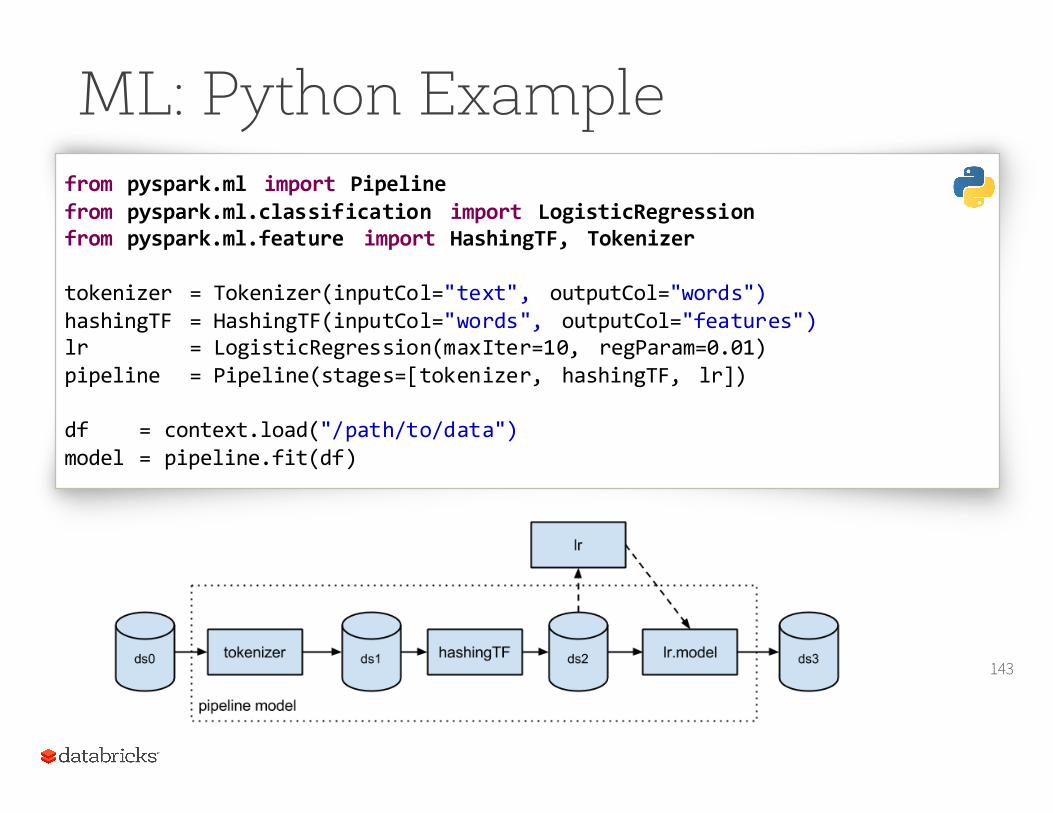
ML: Python Example
143
from pyspark.ml import Pipelinefrom pyspark.ml.classification import LogisticRegressionfrom pyspark.ml.feature import HashingTF, Tokenizer
tokenizer = Tokenizer(inputCol="text", outputCol="words")hashingTF = HashingTF(inputCol="words", outputCol="features")lr = LogisticRegression(maxIter=10, regParam=0.01)pipeline = Pipeline(stages=[tokenizer, hashingTF, lr])
df = context.load("/path/to/data")model = pipeline.fit(df)
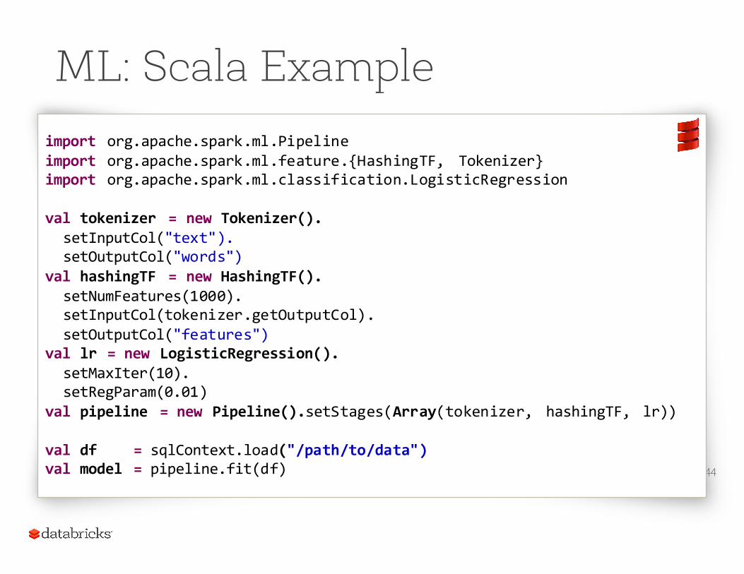
ML: Scala Example
144
import org.apache.spark.ml.Pipelineimport org.apache.spark.ml.feature.{HashingTF, Tokenizer}import org.apache.spark.ml.classification.LogisticRegression
val tokenizer = new Tokenizer().setInputCol("text").setOutputCol("words")
val hashingTF = new HashingTF().setNumFeatures(1000).setInputCol(tokenizer.getOutputCol).setOutputCol("features")
val lr = new LogisticRegression().setMaxIter(10).setRegParam(0.01)
val pipeline = new Pipeline().setStages(Array(tokenizer, hashingTF, lr))
val df = sqlContext.load("/path/to/data")val model = pipeline.fit(df)
Lab
In Databricks, you'll find a DataFrames SQL lab notebook.
•Nominally, it's Python lab• It's based on the previous DataFrames lab.• But, you'll be issuing SQL statements.
•Copy the lab into your Databricks folder.•Open the notebook and follow the instructions. At
the bottom of the lab, you'll find an assignment to be completed.
145
End of DataFrames and Spark SQL Module
Related Documents