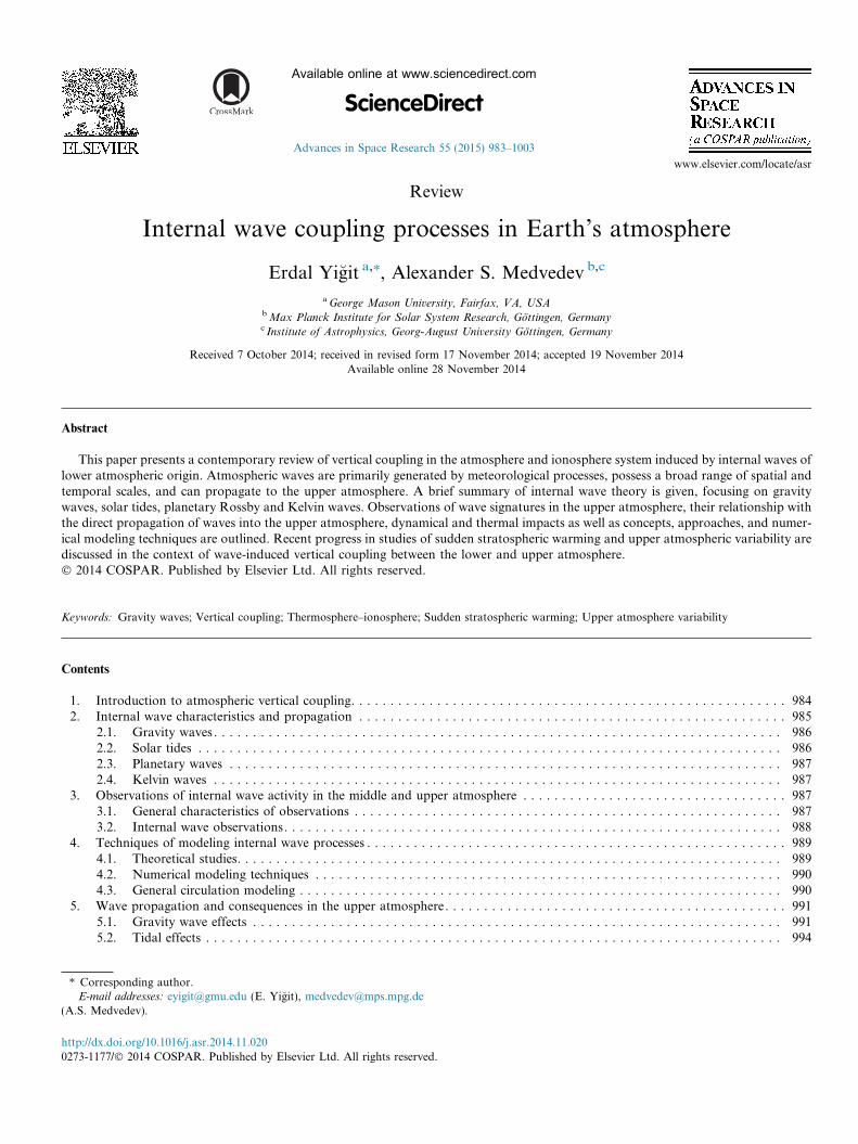
Review Internal wave coupling processes in Earth’s atmosphere Erdal Yig ˘it a,⇑ , Alexander S. Medvedev b,c a George Mason University, Fairfax, VA, USA b Max Planck Institute for Solar System Research, Go ¨ ttingen, Germany c Institute of Astrophysics, Georg-August University Go ¨ ttingen, Germany Received 7 October 2014; received in revised form 17 November 2014; accepted 19 November 2014 Available online 28 November 2014 Abstract This paper presents a contemporary review of vertical coupling in the atmosphere and ionosphere system induced by internal waves of lower atmospheric origin. Atmospheric waves are primarily generated by meteorological processes, possess a broad range of spatial and temporal scales, and can propagate to the upper atmosphere. A brief summary of internal wave theory is given, focusing on gravity waves, solar tides, planetary Rossby and Kelvin waves. Observations of wave signatures in the upper atmosphere, their relationship with the direct propagation of waves into the upper atmosphere, dynamical and thermal impacts as well as concepts, approaches, and numer- ical modeling techniques are outlined. Recent progress in studies of sudden stratospheric warming and upper atmospheric variability are discussed in the context of wave-induced vertical coupling between the lower and upper atmosphere. Ó 2014 COSPAR. Published by Elsevier Ltd. All rights reserved. Keywords: Gravity waves; Vertical coupling; Thermosphere–ionosphere; Sudden stratospheric warming; Upper atmosphere variability Contents 1. Introduction to atmospheric vertical coupling........................................................ 984 2. Internal wave characteristics and propagation ....................................................... 985 2.1. Gravity waves ......................................................................... 986 2.2. Solar tides ........................................................................... 986 2.3. Planetary waves ....................................................................... 987 2.4. Kelvin waves ......................................................................... 987 3. Observations of internal wave activity in the middle and upper atmosphere .................................. 987 3.1. General characteristics of observations ....................................................... 987 3.2. Internal wave observations ................................................................ 988 4. Techniques of modeling internal wave processes ...................................................... 989 4.1. Theoretical studies...................................................................... 989 4.2. Numerical modeling techniques ............................................................ 990 4.3. General circulation modeling .............................................................. 990 5. Wave propagation and consequences in the upper atmosphere ............................................ 991 5.1. Gravity wave effects .................................................................... 991 5.2. Tidal effects .......................................................................... 994 http://dx.doi.org/10.1016/j.asr.2014.11.020 0273-1177/Ó 2014 COSPAR. Published by Elsevier Ltd. All rights reserved. ⇑ Corresponding author. E-mail addresses: [email protected] (E. Yig ˘it), [email protected] (A.S. Medvedev). www.elsevier.com/locate/asr Available online at www.sciencedirect.com ScienceDirect Advances in Space Research 55 (2015) 983–1003

Welcome message from author
This document is posted to help you gain knowledge. Please leave a comment to let me know what you think about it! Share it to your friends and learn new things together.
Transcript
Available online at www.sciencedirect.com
www.elsevier.com/locate/asr
ScienceDirect
Advances in Space Research 55 (2015) 983–1003
Review
Internal wave coupling processes in Earth’s atmosphere
Erdal Yigit a,⇑, Alexander S. Medvedev b,c
a George Mason University, Fairfax, VA, USAb Max Planck Institute for Solar System Research, Gottingen, Germanyc Institute of Astrophysics, Georg-August University Gottingen, Germany
Received 7 October 2014; received in revised form 17 November 2014; accepted 19 November 2014Available online 28 November 2014
Abstract
This paper presents a contemporary review of vertical coupling in the atmosphere and ionosphere system induced by internal waves oflower atmospheric origin. Atmospheric waves are primarily generated by meteorological processes, possess a broad range of spatial andtemporal scales, and can propagate to the upper atmosphere. A brief summary of internal wave theory is given, focusing on gravitywaves, solar tides, planetary Rossby and Kelvin waves. Observations of wave signatures in the upper atmosphere, their relationship withthe direct propagation of waves into the upper atmosphere, dynamical and thermal impacts as well as concepts, approaches, and numer-ical modeling techniques are outlined. Recent progress in studies of sudden stratospheric warming and upper atmospheric variability arediscussed in the context of wave-induced vertical coupling between the lower and upper atmosphere.� 2014 COSPAR. Published by Elsevier Ltd. All rights reserved.
Keywords: Gravity waves; Vertical coupling; Thermosphere–ionosphere; Sudden stratospheric warming; Upper atmosphere variability
Contents
1. Introduction to atmospheric vertical coupling. . . . . . . . . . . . . . . . . . . . . . . . . . . . . . . . . . . . . . . . . . . . . . . . . . . . . . . . 9842. Internal wave characteristics and propagation . . . . . . . . . . . . . . . . . . . . . . . . . . . . . . . . . . . . . . . . . . . . . . . . . . . . . . . 985
http://d
0273-1
⇑ CoE-m
(A.S. M
2.1. Gravity waves . . . . . . . . . . . . . . . . . . . . . . . . . . . . . . . . . . . . . . . . . . . . . . . . . . . . . . . . . . . . . . . . . . . . . . . . . 9862.2. Solar tides . . . . . . . . . . . . . . . . . . . . . . . . . . . . . . . . . . . . . . . . . . . . . . . . . . . . . . . . . . . . . . . . . . . . . . . . . . . 9862.3. Planetary waves . . . . . . . . . . . . . . . . . . . . . . . . . . . . . . . . . . . . . . . . . . . . . . . . . . . . . . . . . . . . . . . . . . . . . . . 9872.4. Kelvin waves . . . . . . . . . . . . . . . . . . . . . . . . . . . . . . . . . . . . . . . . . . . . . . . . . . . . . . . . . . . . . . . . . . . . . . . . . 987
3. Observations of internal wave activity in the middle and upper atmosphere . . . . . . . . . . . . . . . . . . . . . . . . . . . . . . . . . . 987
3.1. General characteristics of observations . . . . . . . . . . . . . . . . . . . . . . . . . . . . . . . . . . . . . . . . . . . . . . . . . . . . . . . 9873.2. Internal wave observations. . . . . . . . . . . . . . . . . . . . . . . . . . . . . . . . . . . . . . . . . . . . . . . . . . . . . . . . . . . . . . . . 9884. Techniques of modeling internal wave processes . . . . . . . . . . . . . . . . . . . . . . . . . . . . . . . . . . . . . . . . . . . . . . . . . . . . . . 989
4.1. Theoretical studies. . . . . . . . . . . . . . . . . . . . . . . . . . . . . . . . . . . . . . . . . . . . . . . . . . . . . . . . . . . . . . . . . . . . . . 9894.2. Numerical modeling techniques . . . . . . . . . . . . . . . . . . . . . . . . . . . . . . . . . . . . . . . . . . . . . . . . . . . . . . . . . . . . 9904.3. General circulation modeling . . . . . . . . . . . . . . . . . . . . . . . . . . . . . . . . . . . . . . . . . . . . . . . . . . . . . . . . . . . . . . 9905. Wave propagation and consequences in the upper atmosphere. . . . . . . . . . . . . . . . . . . . . . . . . . . . . . . . . . . . . . . . . . . . 991
5.1. Gravity wave effects . . . . . . . . . . . . . . . . . . . . . . . . . . . . . . . . . . . . . . . . . . . . . . . . . . . . . . . . . . . . . . . . . . . . 9915.2. Tidal effects . . . . . . . . . . . . . . . . . . . . . . . . . . . . . . . . . . . . . . . . . . . . . . . . . . . . . . . . . . . . . . . . . . . . . . . . . . 994x.doi.org/10.1016/j.asr.2014.11.020
177/� 2014 COSPAR. Published by Elsevier Ltd. All rights reserved.
rresponding author.ail addresses: [email protected] (E. Yigit), [email protected]).
984 E. Yigit, A.S. Medvedev / Advances in Space Research 55 (2015) 983–1003
6. Vertical coupling during sudden stratospheric warmings . . . . . . . . . . . . . . . . . . . . . . . . . . . . . . . . . . . . . . . . . . . . . . . . 9967. Upper atmosphere variability . . . . . . . . . . . . . . . . . . . . . . . . . . . . . . . . . . . . . . . . . . . . . . . . . . . . . . . . . . . . . . . . . . . 9978. Open questions and concluding remarks . . . . . . . . . . . . . . . . . . . . . . . . . . . . . . . . . . . . . . . . . . . . . . . . . . . . . . . . . . . 999
Acknowledgments . . . . . . . . . . . . . . . . . . . . . . . . . . . . . . . . . . . . . . . . . . . . . . . . . . . . . . . . . . . . . . . . . . . . . . . . . . . 999References . . . . . . . . . . . . . . . . . . . . . . . . . . . . . . . . . . . . . . . . . . . . . . . . . . . . . . . . . . . . . . . . . . . . . . . . . . . . . . . . 999
1. Introduction to atmospheric vertical coupling
The structure and dynamics of Earth’s atmosphere aredetermined by a complex interplay of radiative, dynamical,thermal, chemical, and electrodynamical processes in thepresence of solar and geomagnetic activity variations.The lower atmospheric processes are the primary concernof meteorology, while impacts of the Sun and geomagneticprocesses on the atmosphere–ionosphere are the subject ofspace weather research. Thus, the whole atmosphere sys-tem is under the continuous influence of meteorologicaleffects and space weather. A detailed understanding ofthe coupling mechanisms within the atmosphere–iono-sphere is crucial for better interpreting atmospheric obser-vations, understanding the Earth climate system, anddeveloping forecast capabilities.
The atmosphere can be viewed as an ideal geophysicalfluid that is pervaded by waves of various spatio-temporalscales. The term “internal” signifies the ability of waves topropagate “internally”, that is, vertically upward within theatmosphere, unlike “external” modes, in which all layersoscillate in sync when disturbances propagate horizontally.Internal waves exist because Earth’s atmosphere is overallstably stratified. Horizontal scales of internal waves varyfrom a few kilometers to the planetary circumference. Tem-poral scales cover a range from minutes to several days.Internal waves can propagate over large distances, andtransfer momentum and energy from lower levels to muchhigher altitudes, thus providing an important couplingmechanism in the atmosphere. What are the impacts ofthese waves on the atmosphere–ionosphere system at vari-ous scales? The scientific community has increasingly beenrealizing that answering this question represents a crucialstep toward better understanding the connections betweenmeteorology and space weather.
Coupling processes from the lower atmosphere to theionosphere have been the overarching goal of recent obser-vational campaigns. One such campaign was the Spread-FEx that was conducted over the South American sector(Abdu et al., 2009; Takahashi et al., 2009).
Nonlinear interactions of internal waves between them-selves and with the undisturbed atmospheric flow create acomplex dynamical system, in which long-range couplingprocesses can occur that link different atmospheric layersand redistribute energy and momentum between them.To investigate the origins and global consequences of suchprocesses, the atmospheric layers cannot be investigated inisolation, but the atmosphere ought to be treated as awhole system. The importance of such investigations have
been broadly recognized. In the Role Of the Sun and theMiddle atmosphere/thermosphere/ionosphere In Climate(ROSMIC, Lubken et al., 2014) project within the SCO-STEP’s VarSITI (Variability of the Sun and Its TerrestrialImpact) program, the influence of the lower atmosphere onthe upper atmosphere is designated as one of the focus top-ics (Ward et al., 2014). Specifically, ROSMIC’s “Couplingby Dynamics” Working Group coordinates the efforts ininvestigating dynamically-induced vertical coupling pro-cesses in the atmosphere–ionosphere system.
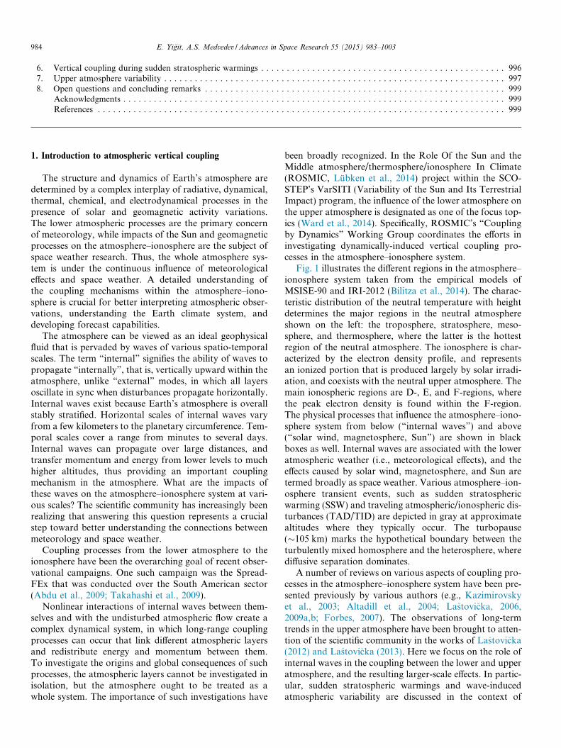
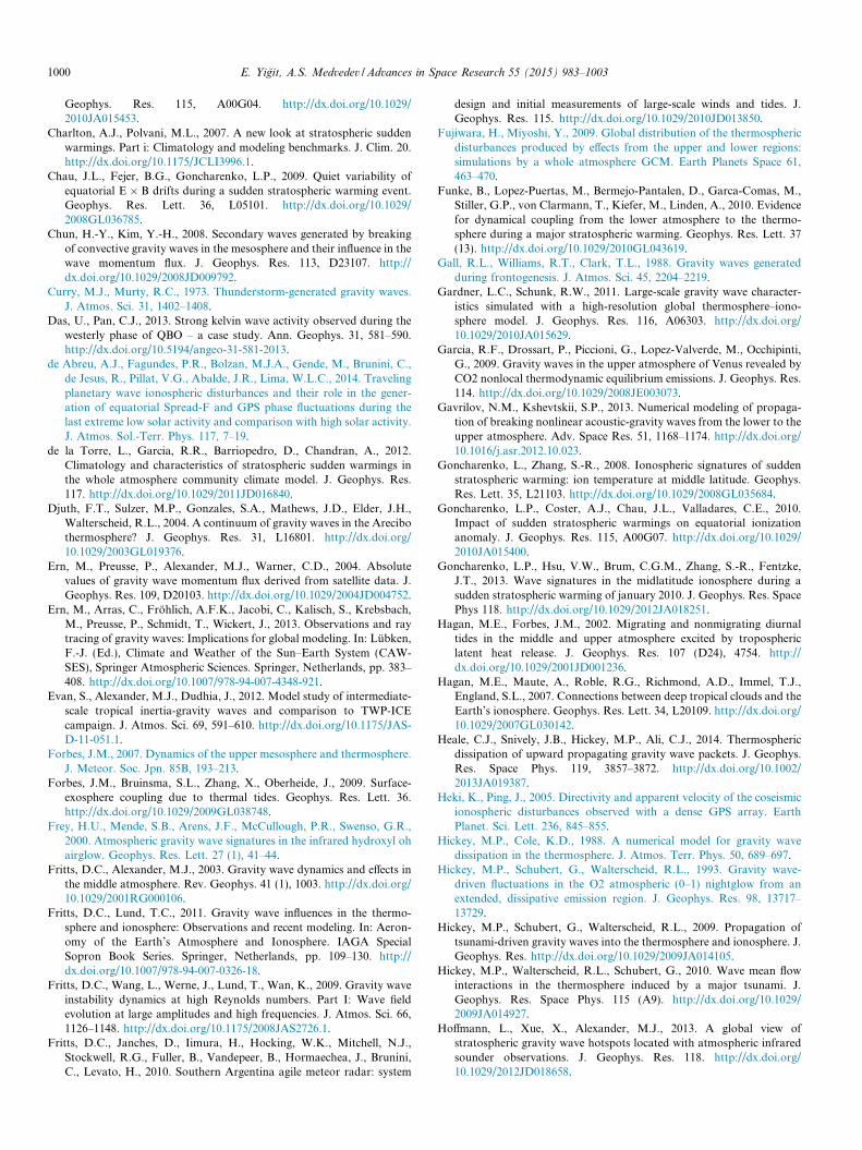
Fig. 1 illustrates the different regions in the atmosphere–ionosphere system taken from the empirical models ofMSISE-90 and IRI-2012 (Bilitza et al., 2014). The charac-teristic distribution of the neutral temperature with heightdetermines the major regions in the neutral atmosphereshown on the left: the troposphere, stratosphere, meso-sphere, and thermosphere, where the latter is the hottestregion of the neutral atmosphere. The ionosphere is char-acterized by the electron density profile, and representsan ionized portion that is produced largely by solar irradi-ation, and coexists with the neutral upper atmosphere. Themain ionospheric regions are D-, E, and F-regions, wherethe peak electron density is found within the F-region.The physical processes that influence the atmosphere–iono-sphere system from below (“internal waves”) and above(“solar wind, magnetosphere, Sun”) are shown in blackboxes as well. Internal waves are associated with the loweratmospheric weather (i.e., meteorological effects), and theeffects caused by solar wind, magnetosphere, and Sun aretermed broadly as space weather. Various atmosphere–ion-osphere transient events, such as sudden stratosphericwarming (SSW) and traveling atmospheric/ionospheric dis-turbances (TAD/TID) are depicted in gray at approximatealtitudes where they typically occur. The turbopause(�105 km) marks the hypothetical boundary between theturbulently mixed homosphere and the heterosphere, wherediffusive separation dominates.
A number of reviews on various aspects of coupling pro-cesses in the atmosphere–ionosphere system have been pre-sented previously by various authors (e.g., Kazimirovskyet al., 2003; Altadill et al., 2004; Lastovicka, 2006,2009a,b; Forbes, 2007). The observations of long-termtrends in the upper atmosphere have been brought to atten-tion of the scientific community in the works of Lastovicka(2012) and Lastovicka (2013). Here we focus on the role ofinternal waves in the coupling between the lower and upperatmosphere, and the resulting larger-scale effects. In partic-ular, sudden stratospheric warmings and wave-inducedatmospheric variability are discussed in the context of
100 200 300 400 500 600 700 800
100
200
300
400
500
Space Weather
TAD/TID
SSWWeather
Neutral Temperature [K]
0
Alti
tude
[km
]
Troposphere
Stratosphere
Mesosphere
Thermosphere
Turbopause
Internal Waves
Solar Wind, Magnetosphere, Sun
108 109 1010 1011 1012 1013
Electron Density [m-3]
F-region
E-region
D-region
Iono
sphe
re
Fig. 1. Vertical structure of the atmosphere–ionosphere system, where the neutral atmospheric temperature is shown on the left and the electron densitydistribution on the right. Panels are produced using midlatitude data from MSISE-90 and IRI 2012 models for 1 January 2010 at noon with dailyF 10:7 ¼ 77:2� 10�22 W m�2 Hz�1 and Ap ¼ 0:5. SSW and TAD/TID denotes sudden stratospheric warming and traveling atmospheric/ionosphericdisturbances, respectively. The turbopause is at about 105 km.
Table 1Typical temporal scales of internal waves in the terrestrial atmosphere.
Internal wave Typical range of temporal scales
Gravity wave Few minutes to several hours (2p=f ; f ¼ 2X sin /)Solar tide 1, 1/2, 1/3 daysPlanetary wave 2 to few tens of daysKelvin wave 3 to 20 days
E. Yigit, A.S. Medvedev / Advances in Space Research 55 (2015) 983–1003 985
vertical coupling, as the two topics have recently comeagain to the meteorology and aeronomy communities’attention. Our overarching goal is to provide a motivationfor bridging gaps between scientists studying the lower,middle, and upper atmospheres. In this paper, we concen-trate on the most recent studies, while providing referencesto the existing reviews for further details.
This review is structured in the following manner. Sec-tion 2 provides an overview of the physical properties ofinternal waves. Section 3 outlines the observations of wavestructures in the middle and upper atmosphere. Section 4presents modeling techniques for studying internal waves,and Section 5 gives some details concerning atmosphericwave propagation and consequences for the upper atmo-sphere. Sections 6 and 7 discuss coupling processes duringsudden stratospheric warmings (SSWs), and other effectsrelated to upper atmosphere variability. In Section 8, conclu-sions are given, and some open questions are highlighted.
2. Internal wave characteristics and propagation
To a first approximation, atmospheric waves can be dis-tinguished by their spatial scales. Earth’s atmosphere pos-sesses a broad spectrum of waves ranging from verysmall- (e.g., gravity waves, GWs) to planetary-scale waves(tides, Rossby waves). Table 1 summarizes quantitativelythe range of temporal scales for tides, gravity, planetary
Rossby and Kelvin waves. Overall, internal wave periodsvary from a few minutes to tens of days. They also have dif-ferent spatial scales. While small-scale GWs have typicalhorizontal wavelengths kH of several km to several hundredkm, horizontal scales of solar tides and planetary waves arecomparable to the circumference of Earth.
Although various internal waves can be excited by dif-ferent mechanisms, in general, meteorological processesare the primary sources of these motions. They can propa-gate upward and grow in amplitude due to exponentiallydecreasing neutral mass density q (in order to satisfy waveaction conservation). Therefore, although wave distur-bances associated with small-scale GWs are relatively smallat the source levels, their amplitudes can become significantat higher altitudes in the thermosphere, and are all subjectto various dissipation processes. On the other hand, large-scale waves, such as planetary waves, can possess relativelylarger amplitudes in the lower atmosphere, and can, there-fore, dissipate at lower altitudes. This wave dissipation is
986 E. Yigit, A.S. Medvedev / Advances in Space Research 55 (2015) 983–1003
the mechanism of transfer of momentum and energy fromdisturbances to the mean flow. Below, a brief characteriza-tion of some internal waves is presented.
2.1. Gravity waves
These waves have a broad range of scales from small-scale acoustic-gravity waves to large-scale inertia-gravitywaves. They are routinely seen in lidar, radar, airglow,and satellite measurements. Generated typically in thelower atmosphere by meteorological processes, such asconvection (Song et al., 2003), frontogenesis (Gall et al.,1988), nonlinear interactions (Medvedev and Gavrilov,1995), and thunderstorms (Curry and Murty, 1973), theycan propagate upward to the middle and upper atmo-sphere. These sources produce broad spatial and temporalspectra of GWs in the lower atmosphere. The spectra typ-ically describe quadratic (with respect to disturbances)quantities: energy, wave action, or momentum fluxes(u0w0, v0w0) as functions of horizontal phase speeds c, orother spectral parameters. The fluxes u0w0 and v0w0 denotethe vertical fluxes of the wave zonal and meridionalmomentum, respectively. The vertical structure of fluxesassociated with a GW harmonic i can be written as (e.g.,Yigit et al., 2008):
F ¼ u0w0iðzÞv0w0iðzÞ
( )¼ u0w0iðz0Þ
v0w0iðz0Þ
( )� qðz0Þ
qðzÞ siðzÞ; ð1Þ
where z0 denotes the source level;qðzÞ ¼ qðz0Þ exp½�ðz� z0Þ=H � is the background neutralmass density, H is the scale height, and si is the transmissiv-ity function for the ith harmonic. Eq. (1) implies that thewave momentum flux grows exponentially with height z
above the source level z0. As GWs propagate upward, theyinteract with the atmospheric background continuously.The mean flow affects the propagation of GWs by modify-ing the transmissivity, which is given for one harmonic by
siðzÞ ¼ exp �Z z
z0
Xd
bidðz0Þdz0
" #; ð2Þ
where bid is the dissipation of wave harmonic i due to a
given attenuation process denoted by d. The total dissipa-tion is the sum of all attenuation processes taking placesimultaneously:
btotðzÞ ¼ bionðzÞ þ bmolðzÞ þ beddyðzÞ þ bnonðzÞ þ bradðzÞ; ð3Þ
where the height-dependent total dissipation btotðzÞ is a sumof dissipations due to ion drag, molecular diffusion andthermal conduction (Vadas and Fritts, 2005), eddy diffu-sion, nonlinear diffusion (Weinstock, 1982; Medvedevand Klaassen, 1995, 2000), and radiative damping(Holton, 1982), as introduced in the work by Yigit et al.(2008).
As seen from (1)–(3), upward GW propagation isaffected by a competition between the nearly exponentialgrowth of the momentum flux F, and dissipation acting
upon the wave. This process facilitates a continuous trans-fer of the wave momentum and energy to the mean flow.The resulting dynamical effect a on the flow represents abody force per unit mass, that is, the acceleration/deceler-ation of the mean flow, which is given by the divergenceof the momentum flux F:
aðzÞ ¼ � 1
q@qFðzÞ@z
: ð4Þ
Thermal effects originating from GWs are described byheating/cooling rates per unit mass. The total thermal effectcomprises an irreversible heating E due to transfer ofmechanical energy into heat, and the differential heating/cooling Q caused by the downward transport of the sensi-ble heat flux w0T 0:
QðzÞ ¼ � 1
q@qw0T 0
@z; ð5Þ
T 0 being wave-induced temperature disturbances(Medvedev and Klaassen, 2003; Becker, 2004; Yigit andMedvedev, 2009). The very same formalism for calculatingdynamical and thermal effects can be applied to solar tides,planetary and Kelvin waves described below.
2.2. Solar tides
Solar tides are particular types of gravity waves forcedby periodic heating associated with the absorption of solarradiation in the atmosphere. The obvious period is 24 h,however, due to the nonlinearity of the atmosphericdynamics, higher-order harmonics with frequenciesxn ¼ nX, X ¼ 2p=24 h (n ¼ 2; 3, etc.) are also excited.The first few tidal harmonics (diurnal, semidiurnal, and ter-diurnal) are abundant in the middle atmosphere, and havenoticeable amplitudes. Tidal disturbances can be repre-sented globally with the Fourier series as a sum ofharmonics
Ans cos ðnXt þ skþ /nsÞ; ð6Þ
where k is the longitude, s ¼ 0;�1;�2; . . . is the zonalwavenumber, and Ans and /ns are the amplitude and phase,correspondingly. Eastward and westward propagation cor-respond to s < 0 and s > 0, respectively. Eq. (6) can berewritten in terms of the local time tLT ¼ t þ k=X as
Ans cos ½nXtLT þ ðs� nÞkþ /ns�: ð7Þ
The nomenclature of tides follows from (7). If s ¼ n, oscil-lations are Sun-synchronous (that is, waves move westwardfollowing the apparent motion of the Sun), and such modesare called “migrating tides”. Harmonics with s – n arenon-migrating tides, which can move either westward oreastward (depending on s and n). Such harmonics areexcited due to inhomogeneity of solar radiation absorptionand nonlinearity of atmospheric motions.
Tides have distinctive meridional structures defined bytheir propagation properties. Under the approximation ofa linear, motionless, isothermal, and inviscid atmosphere,
E. Yigit, A.S. Medvedev / Advances in Space Research 55 (2015) 983–1003 987
the horizonal structure of tides can be conveniently repre-sented as a sum of the so-called Hough functions compris-ing symmetric and antisymmetric with respect to theequator modes. In the real atmosphere, the fundamentaltidal structure no longer coincides with the Hough func-tions. In a practical sense, however, they are still sometimesused in data analyses, because only a few Hough modescan provide a good fit for the tidal component.
As with all gravity waves, only tides, whose intrinsic fre-quency x ¼ xn � s�uða cos /Þ�1 (a being the Earth radius, /is the latitude, �u is the zonally averaged wind) exceeds thelocal Coriolis frequency f ¼ 2X sin /, can propagate verti-cally and produce an effective coupling. For instance, thelower-frequency diurnal tide can propagate from tropo-spheric heights into the upper atmosphere mainly at low-latitudes (subject to the local winds �u), and is verticallytrapped and rapidly decays above the excitation levels athigher latitudes. Tides are observed in the middle atmo-sphere and thermosphere, where they play a profound rolein maintaining atmospheric variability. At the heights ofthe F region, strong in situ thermal tides are forced bythe periodic heating due to absorption of solar UV andEUV radiation. These tides have a barotropic structure(no phase shift in vertical), and the diurnal mode domi-nates. More on the importance of tides in the upper atmo-sphere can be found in the review paper of Forbes (2007).
2.3. Planetary waves
Planetary waves are often a synonym of Rossby waves,which appear in the atmosphere due to the latitudinal gra-dient of the Coriolis force that balances variations of thepressure gradient force. Their phase speed is always west-ward, however the group velocity can have either direction.Planetary waves manifest themselves as a meandering of jetstreams, where the number of meanders gives the zonalwavenumber. Rossby waves are strongly dispersive: thosehaving faster speeds are usually trapped and do not prop-agate vertically. They are called “barotropic” modes,unlike the slower moving “baroclinic” harmonics withzonal wave speeds of few cm s�1. They are excited by theinstability of the tropospheric jet: barotropic (due to a hor-izontal wind shear) or baroclinic one (due to a vertical windshear), correspondingly. The slowest planetary waves withthe horizontal wavenumber 1 and/or 2, which are locked toparticular locations, are called “quasi-stationary” waves,and are forced by surface inhomogeneities – topographyand/or surface temperature. According to the dispersionrelation for Rossby waves, which involves the backgroundzonal wind velocity, the quasi-stationary waves have higherchances of propagating into the middle atmosphere anddepositing their momentum and energy upon dissipation,mostly in the winter hemisphere, Rossby waves occur atmiddle- and high-latitudes, although they sometimes canshift to lower latitudes, and even cross the equator(Medvedev et al., 1992). Planetary waves play a profoundrole in the dynamics of the stratosphere. In particular,
the wave momentum they deposit drives the pole-to-polecirculation. Another well-known transient phenomenonassociated with planetary waves are sudden stratosphericwarmings (see section 6). Higher in the atmosphere, thedynamical importance of Rossby waves reduces leaving itto gravity waves.
2.4. Kelvin waves
Atmospheric Kelvin waves are large-scale waves that arethe results of balancing the Coriolis force against the wave-guide at the equator. These waves are trapped at low lati-tudes, their amplitudes decay steeply away from theequator, and their meridional velocity component vanishes,while the zonal one fluctuates. An important feature of Kel-vin waves is that they are non-dispersive, that is, the phasespeed of the wave crests is equal to the group velocity at allfrequencies. The second peculiarity of atmospheric Kelvinwaves is that their phase velocity is positive. Thus, Kelvinwave disturbances always propagate eastward retainingtheir shapes, which is a great help in detecting them.
Kelvin waves are excited by convection in the loweratmosphere, and can propagate vertically. As they dissipatein upper layers, the westerly momentum they depositaffects the mean circulation. Kelvin wave classificationincludes slow (periods of 10 to 20 days), fast (6 to 10 days),and ultra-fast (3 to 5 days). Slow waves play an importantrole in the lower stratosphere dynamics, e.g., in forcing thequasi-biennial oscillation, fast are noticeable in the entirestratosphere, while ultra-fast harmonics can reach themesosphere and thermosphere heights, providing the cou-pling of the latter with the equatorial lower atmosphere.A good review of recent observations and effects of Kelvinwaves in the middle and upper atmosphere can be found inthe introduction of the paper by Das and Pan (2013).
3. Observations of internal wave activity in the middle and
upper atmosphere
3.1. General characteristics of observations
A variety of techniques is utilized to detect wave signa-tures in the atmosphere. To date, a combination of in situ
and remote sensing observational methods provides anunprecedented view of the local and global state and com-position of the atmosphere. Thus, atmospheric tempera-ture, pressure, wind fields, humidity, solar radiation flux,trace substances, electrical properties, and precipitationcan be observed by these techniques. A variety of small-and large-scale structures can be identified in the measuredfields, which exhibit systematic wave-like variations and,thus, are indicative of wave propagation. As more techno-logically sophisticated instruments with higher resolutionsare built, the capability of capturing finer structuresincreases.
The key general characteristics of observations are error,accuracy, resolution, and signal-to-noise ratio. An error
(a)
(b)
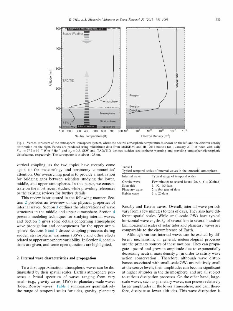
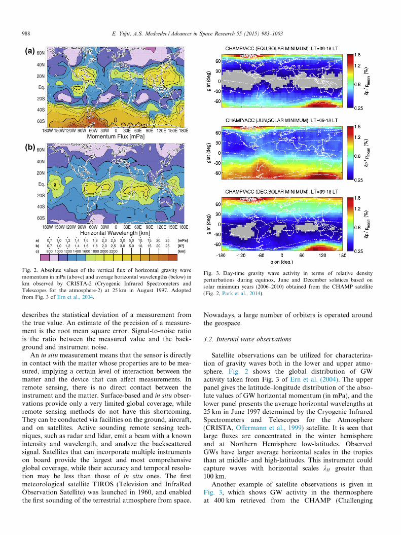
Fig. 2. Absolute values of the vertical flux of horizontal gravity wavemomentum in mPa (above) and average horizontal wavelengths (below) inkm observed by CRISTA-2 (Cryogenic Infrared Spectrometers andTelescopes for the atmosphere-2) at 25 km in August 1997. Adoptedfrom Fig. 3 of Ern et al., 2004.
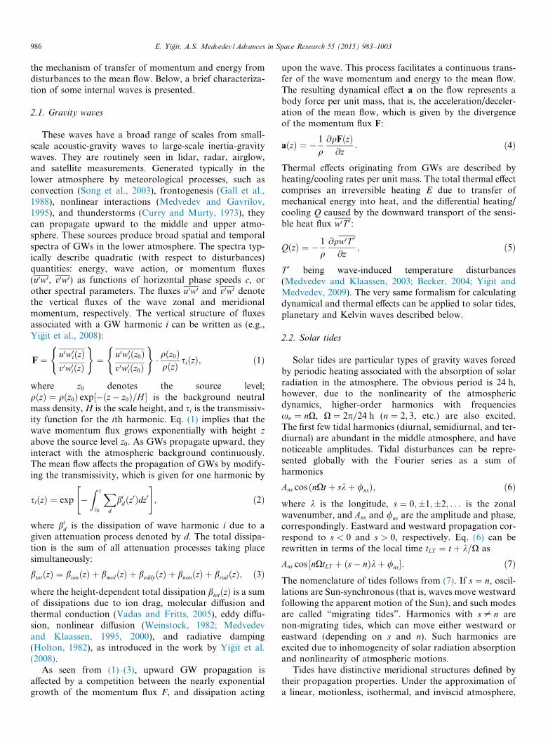
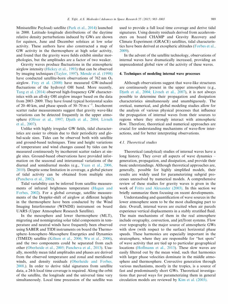
Fig. 3. Day-time gravity wave activity in terms of relative densityperturbations during equinox, June and December solstices based onsolar minimum years (2006–2010) obtained from the CHAMP satellite(Fig. 2, Park et al., 2014).
988 E. Yigit, A.S. Medvedev / Advances in Space Research 55 (2015) 983–1003
describes the statistical deviation of a measurement fromthe true value. An estimate of the precision of a measure-ment is the root mean square error. Signal-to-noise ratiois the ratio between the measured value and the back-ground and instrument noise.
An in situ measurement means that the sensor is directlyin contact with the matter whose properties are to be mea-sured, implying a certain level of interaction between thematter and the device that can affect measurements. Inremote sensing, there is no direct contact between theinstrument and the matter. Surface-based and in situ obser-vations provide only a very limited global coverage, whileremote sensing methods do not have this shortcoming.They can be conducted via facilities on the ground, aircraft,and on satellites. Active sounding remote sensing tech-niques, such as radar and lidar, emit a beam with a knownintensity and wavelength, and analyze the backscatteredsignal. Satellites that can incorporate multiple instrumentson board provide the largest and most comprehensiveglobal coverage, while their accuracy and temporal resolu-tion may be less than those of in situ ones. The firstmeteorological satellite TIROS (Television and InfraRedObservation Satellite) was launched in 1960, and enabledthe first sounding of the terrestrial atmosphere from space.
Nowadays, a large number of orbiters is operated aroundthe geospace.
3.2. Internal wave observations
Satellite observations can be utilized for characteriza-tion of gravity waves both in the lower and upper atmo-sphere. Fig. 2 shows the global distribution of GWactivity taken from Fig. 3 of Ern et al. (2004). The upperpanel gives the latitude–longitude distribution of the abso-lute values of GW horizontal momentum (in mPa), and thelower panel presents the average horizontal wavelengths at25 km in June 1997 determined by the Cryogenic InfraredSpectrometers and Telescopes for the Atmosphere(CRISTA, Offermann et al., 1999) satellite. It is seen thatlarge fluxes are concentrated in the winter hemisphereand at Northern Hemisphere low-latitudes. ObservedGWs have larger average horizontal scales in the tropicsthan at middle- and high-latitudes. This instrument couldcapture waves with horizontal scales kH greater than100 km.
Another example of satellite observations is given inFig. 3, which shows GW activity in the thermosphereat 400 km retrieved from the CHAMP (Challenging
E. Yigit, A.S. Medvedev / Advances in Space Research 55 (2015) 983–1003 989
Minisatellite Payload) satellite (Park et al., 2014) launchedin 2000. Latitude–longitude distributions of the daytimerelative density perturbations induced by GWs are shownfor equinox, June and December solstices at low solaractivity. These authors have also constructed a map ofGW activity in the thermosphere at high solar activity,and found that the gravity wave fields exhibit similar mor-phologies, but the amplitudes are a factor of two weaker.
Gravity waves produce fluctuations in the atmosphericairglow intensity (Hickey et al., 1993) that can be observedby imaging techniques (Taylor, 1997). Mende et al. (1998)have conducted satellite-born observations of 762 nm O2
airglow. Frey et al. (2000) have measured GW-inducedfluctuations of the hydroxyl OH band. More recently,Tang et al. (2014) observed high-frequency GW character-istics with an all-sky OH airglow imager based on the datafrom 2003–2009. They have found typical horizontal scalesof 20–40 km, and phase speeds of 30–70 m s�1. Incoherentscatter radar measurements suggest that gravity wave-likevariations can be detected frequently in the upper atmo-sphere (Oliver et al., 1997; Djuth et al., 2004; Livnehet al., 2007).
Unlike with highly irregular GW fields, tidal character-istics are easier to obtain due to their periodicity and glo-bal-scale sizes. Tides can be observed both with satelliteand ground-based techniques. Time and height variationsof temperature and wind changes caused by tides can bemeasured continuously by incoherent scatter radars at sin-gle sites. Ground-based observations have provided infor-mation on the seasonal and interannual variations of thediurnal and semidiurnal modes (e.g., Yuan et al., 2006,2010). Despite some limitation in coverage, a global pictureof tidal activity can be obtained from multiple sites(Pancheva et al., 2002).
Tidal variability can be inferred from satellite measure-ments of infrared brightness temperature (Hagan andForbes, 2002). For a global coverage, satellite measure-ments of the Doppler-shift of airglow at different heightsin the thermosphere have been conducted by the WindImaging Interferometer (WINDII) instrument on boardUARS (Upper Atmosphere Research Satellite).
In the mesosphere and lower thermosphere (MLT),migrating and nonmigrating solar tidal components in tem-perature and neutral winds have frequently been observedusing SABER and TIDI instruments on board the Thermo-sphere–Ionosphere–Mesosphere Energetics and Dynamics(TIMED) satellite (Killeen et al., 2006; Wu et al., 2006),and the two components could be separated from eachother (Oberheide et al., 2005; Pancheva et al., 2013). Usu-ally, monthly mean tidal amplitudes and phases are derivedfrom the observed temperature and zonal and meridionalwinds, and density residuals (Oberheide and Forbes,2008,). In order to derive tidal signatures from satellitedata, a 24-h local time coverage is required. Along the orbitof the satellite, the longitude and the universal time varysimultaneously. Local time precession of the satellite was
used to provide a full local time coverage and derive tidalsignatures. Using density residuals derived from accelerom-eters on board CHAMP and Gravity Recovery andClimate Experiment (GRACE) satellites, tidal characteris-tics have been derived at exospheric altitudes (Forbes et al.,2009).
In the advent of the satellite technology, observations ofinternal waves have dramatically increased, providing anunprecedented global view of the activity of these waves.
4. Techniques of modeling internal wave processes
Although observations suggest that wave-like structuresare continuously present in the upper atmosphere (e.g.,Djuth et al., 2004; Livneh et al., 2007), it is not alwayspossible to determine their propagation and dissipationcharacteristics simultaneously and unambiguously. Theoretical, numerical, and global modeling studies allow forthe analysis of various physical processes that influencethe propagation of internal waves from their sources toregions where they strongly interact with atmosphericflow. Therefore, theoretical and numerical approaches arecrucial for understanding mechanisms of wave-flow inter-actions, and for better interpreting observations.
4.1. Theoretical studies
Theoretical (analytical) studies of internal waves have along history. They cover all aspects of wave dynamics –generation, propagation, and dissipation, and provide theirbasic understandings. Although theoretical approaches are,generally, possible for highly simplified models, theirresults are widely used for parameterizing subgrid pro-cesses unresolved by numerical models. A comprehensivereview of these studies for gravity waves is given in thework of Fritts and Alexander (2003). In this section webriefly summarize them focusing on recent developments.
Understanding and quantification of wave sources in thelower atmosphere seem to be the most challenging part todate. Overall, internal waves are excited when air parcelsexperience vertical displacements in a stably stratified fluid.The main mechanisms of them in the real atmosphereinclude orography, convection, and jet/front systems. Flowover topography is the major source of atmospheric GWswith slow (with respect to the surface) horizontal phasespeeds. These harmonics are especially important in thestratosphere, where they are responsible for “hot spots”
of wave activity that are tied up to particular geographicallocations (Hoffmann et al., 2013). These slow waves areeasily filtered out by the mean wind, such that harmonicswith larger phase velocities dominate in the middle atmo-sphere and thermosphere. Convective generation throughvarious mechanisms, mostly in the tropics, is a source offast and predominantly short GWs. Theoretical investiga-tions that paved ways for parameterizing them in generalcirculation models are reviewed by Kim et al. (2003).
990 E. Yigit, A.S. Medvedev / Advances in Space Research 55 (2015) 983–1003
GWs are ubiquitous in the middle and upper atmo-sphere, and are not limited to low latitudes and/or partic-ular hotspots. Tropospheric jet/front systems areidentified as the main source of these waves. Although ver-tical displacements of air parcels in jets and fronts are obvi-ously responsible for generation, the exact mechanismthrough which GWs are excited is not known, and is a sub-ject of intense theoretical studies. The main candidates aregeostrophic adjustment, Lighthill radiation, various insta-bilities and transient generation. Geostrophic adjustmentimplies a presence of GWs superimposed on a slower andmore “balanced” flow. This leaves out the question ofwhy they are present at first hand by simply stating thatthis is a fundamental property of the flow. Other theoreti-cal mechanisms strive to explain this. Lighthill radiationmechanism of GWs is based on an analogy with the gener-ation of acoustic waves by vortical turbulent motions. Inthe heart of it lies the nonlinearity of flows, by means ofwhich energy from slower vortical modes is transferred tofast divergent ones (gravity waves). The two mechanismscan probably be related if one extends the geostrophicadjustment to include nonlinearity. With that, a continu-ous competition occurs between the tendencies to distortthe flow from a balanced state due to nonlinear advection,and to restore it by excitation of GWs. Remarkably, thisapproach yields results similar to the Lighthill expressionsfor wave sources (Medvedev and Gavrilov, 1995). A con-ceptually close, but analytically different approach is takenby proponents of the so-called mechanism of “spontaneousadjustment emission”. One more line of theoreticalresearch is related to “unbalanced” instabilities, that is,such conditions under which balanced flows still remainstable, but the present infinitesimal GWs become explo-sively unstable. Transient generation mechanism is concep-tually close to the unbalanced instabilities, but assumesthat amplitudes of thus generated waves can be predictedwithin the linear theory. An excellent and insightful reviewof these theoretical developments has recently been givenby Plougonven and Zhang (2014).
4.2. Numerical modeling techniques
Numerical modeling allows for studying wave processesunder more realistic and complex conditions. Two majortechniques include (1) ray tracing, and (2) direct hydrody-namical simulations. Ray tracing is the least computation-ally expensive among them. It calculates paths of narrowwave packets centered around a harmonic with the givenfrequency and wavenumber through regions with varyingpropagation conditions. The information on wave phasesis lost under this approach, and the entire field can be rep-resented as a collection of a large number of wave packetsand the corresponding very narrow beams (rays). Thistechnique has its limitations. First, it is applicable only ifthe background varies slowly both spatially and temporally(compared to the wavelength and period of a given
harmonic, correspondingly), and, thus, cannot be usedfor studying processes like wave break-up or nonlinearinteractions. Secondly, because no information on wavephases exists, processes like diffraction and interferencecannot be studied with the ray-tracing techniques. More-over, mathematical singularities called “caustics” may arisewhen ray paths of different packets come close. The advan-tage of the ray tracing method is that trajectories areinvariant in time, that is, it can be applied to studyingpropagation of wave packets from their sources as wellas for identification of sources by tracking their paths backin time. These approaches constitute direct and reverse raytracing techniques, respectively. They are widely employedfor interpretation of observations and linking wave signa-tures in the upper atmosphere to sources in the troposphere(e.g., Evan et al., 2012; Paulino et al., 2012, 2014). A con-venience of the ray tracing technique is that the same modelcan be used in both modes (Vadas and Fritts, 2009; Vadaset al., 2009). More on the application of the ray-tracingGW observations and implications for modeling can befound in the paper of Ern et al. (2013).
The method of direct wave simulation is based onnumerical solution of the fundamental (primitive) equa-tions of hydrodynamics, and, therefore, does not have manylimitations of the ray tracing. It allows one to study variousaspects of wave propagation in the entire atmosphere,including the upper thermosphere, where molecular diffu-sion and ion friction substantially alter the physics of waves.Normally, the hydrodynamic equations are linearized withrespect to the larger-scale mean flow (still retaining nonlin-ear terms for disturbances). This formalism permits simula-tions of propagation, refraction, ducting, critical layerfiltering and dissipation of internal waves under a varietyof realistic background distributions of wind and tempera-ture (e.g., Liu et al., 2013; Yua et al., 2009). In certain cases,direct wave models can be applied to studying wave propa-gation from particular sources like tsunami (Occhipintiet al., 2011), or earthquakes (Matsumura et al., 2011).Increasing computing power enables a consideration ofweak nonlinear interactions between harmonics (Huanget al., 2014), their break-ups (Gavrilov and Kshevtskii,2013), and even turbulence formation (Fritts et al., 2009).The main challenge with the direct wave simulation methodcomes from the fact that GWs may have fast phase speeds,integration requires a long time, and model domains musthave significant sizes. This problem is usually circumventedby imposing periodic lateral boundary conditions, whichprevent the accounting for dispersion of wave packets.Extending domains of integration brings the direct wavemodels closer to another class of numerical tools, namelyto general circulation models.
4.3. General circulation modeling
General circulation models or Global Climate Models(GCMs) are three-dimensional (3-D) complex mathematical
E. Yigit, A.S. Medvedev / Advances in Space Research 55 (2015) 983–1003 991
models that solve the fundamental equations of motion,energy, and continuity on a sphere. The numerical solutionsof the conservation equations enable a simulation of theatmospheric dynamics, and an investigation of their interac-tions with the underlying physical, chemical, and radiativeprocesses. The progress with digital computers in the secondhalf of the 20th century have prompted the success of GCMsas research tools. The primitive equations are discretizedand then solved numerically to simulate temporal evolutionof atmospheric fields, such as wind, temperature, and den-sity/pressure, under various boundary and external forcingconditions. In GCMs extending into the ionosphere, conser-vation equations for the plasma are solved in addition to theneutrals (e.g., Gardner and Schunk, 2011, 2012).
Depending on the regions of the atmosphere covered byGCMs, they can either be global or limited-area ones.GCMs are also distinguished by the vertical layers theyfocus on: lower/middle atmosphere-, upper atmosphere-and “whole atmosphere” models. In general, lower/middleatmosphere models typically extend from the ground up tothe mesosphere or lower thermosphere (e.g., Manzini et al.,2006); upper atmosphere models cover the thermosphere–ionosphere from the mesopause to exobase (e.g., Gardnerand Schunk, 2011). Whole atmosphere models are beingincreasingly developed, and, as the name suggests, theyperform calculations from the surface or lower atmosphereto the upper thermosphere (e.g., Liu et al., 2010). The hor-izontal and vertical resolutions combined with the assumedtime step define the spatio-temporal capabilities of a GCM.
GCMs provide a variety of advantages. One of them isthe ability to conduct control simulations. In the real atmo-sphere, physical processes occur simultaneously, and isolat-ing individual processes is a challenging task. In a model,one can selectively turn on and off physical processes todetermine their significance. Therefore, GCMs are usefultools for aiding the interpretation of observations. GCMoutput is easier to analyze because it contains all simulatedfields, unlike with observations, which are always limited tocertain parameters and incomplete.
However, no scientific tool comes without shortcom-ings. First, GCMs do not exactly solve the original partialdifferential equations, but their algebraic approximationson a finite number of grid points, or elements, or spectralharmonics. Therefore, it is important that numerical meth-ods are verified to ensure stability and convergence ofnumerical solutions to physical ones, and the model resultsmust be validated. Because temporal and spatial resolu-tions of GCMs are limited, there are always scales ofmotions that cannot be properly resolved, and thesubgrid-scale processes have to be accounted for, or“parameterized”. For that, any type of physics that is notself-consistently captured in GCMs should be mathemati-cally described, ideally from first principles. Some examplesof parameterizations in models are cloud microphysics,convection, eddy diffusion, and gravity waves.
Older as well as many current GCMs used relativelycoarse horizontal grids, typically, a few degrees in
longitude and latitude. Such resolutions are sufficient formodeling large-scale waves such as solar tides, planetaryand Kelvin waves, however, they are inadequate for repro-ducing smaller-scale GWs. This prompted the developmentof GW parameterizations, among which the first were ofLindzen (1981) and Matsuno (1982). The progress in com-putational capabilities facilitates enhancing model resolu-tions, thus enabling GCMs to capture larger portions ofsmall-scale GWs. For instance, Tomikawa et al. (2012)have used a GCM with a T213 spectral truncation, whichcorrespond to a 0.5625� longitude–latitude resolution.
Overall, state-of-the-art GCMs become increasinglymore sophisticated and complex in comparison with theirpredecessors. They include more physical processes, higherresolution to capture dynamics at smaller scales, and canbe coupled together with other numerical models to formso-called “climate system models”. An example of suchmodel, are whole atmosphere GCMs extending from the sur-face to the upper thermosphere (e.g., Liu et al., 2010, 2013).
Development of GCMs requires extensive efforts, typi-cally by a group of researchers. There are community mod-els that are available to a broader community. NationalCenter for Atmospheric Research (NCAR) CommunityClimate System Model is freely available to scientistsworldwide. Extensive support is provided to help guideusers. This modeling framework is a product of collabora-tion between researchers at NCAR and their national andinternational collaborators. On the other hand, there aremodels that originate from a specific research group. Forexample, the Ground-to-topside Model of Atmosphereand Ionosphere for Aeronomy (GAIA) is a full atmo-sphere–ionosphere model that has been developed atKyushu University.
Some applications of numerical and GCM methods inthe context of the investigations of wave effects in the upperatmosphere are presented in the next section.
5. Wave propagation and consequences in the upper
atmosphere
Internal waves affect the momentum, energy, and com-position balance of the middle atmosphere through a vari-ety of effects (e.g., see reviews by Fritts and Alexander,2003; Becker, 2011). Observational and modeling studieshave shown that small-scale GWs (e.g., Yigit et al., 2009)and solar tides (e.g., Oberheide et al., 2009) can directlypropagate to the upper atmosphere as well. We next focuson the upward propagation of these waves from the loweratmosphere to the thermosphere–ionosphere system, andthe resulting effects.
5.1. Gravity wave effects
Earlier studies extensively employed theoretical calcula-tions and numerical simulations to characterize GW prop-agation and dissipation in the thermosphere–ionosphere(Volland, 1969; Hooke, 1970; Klostermeyer, 1972; Hickey
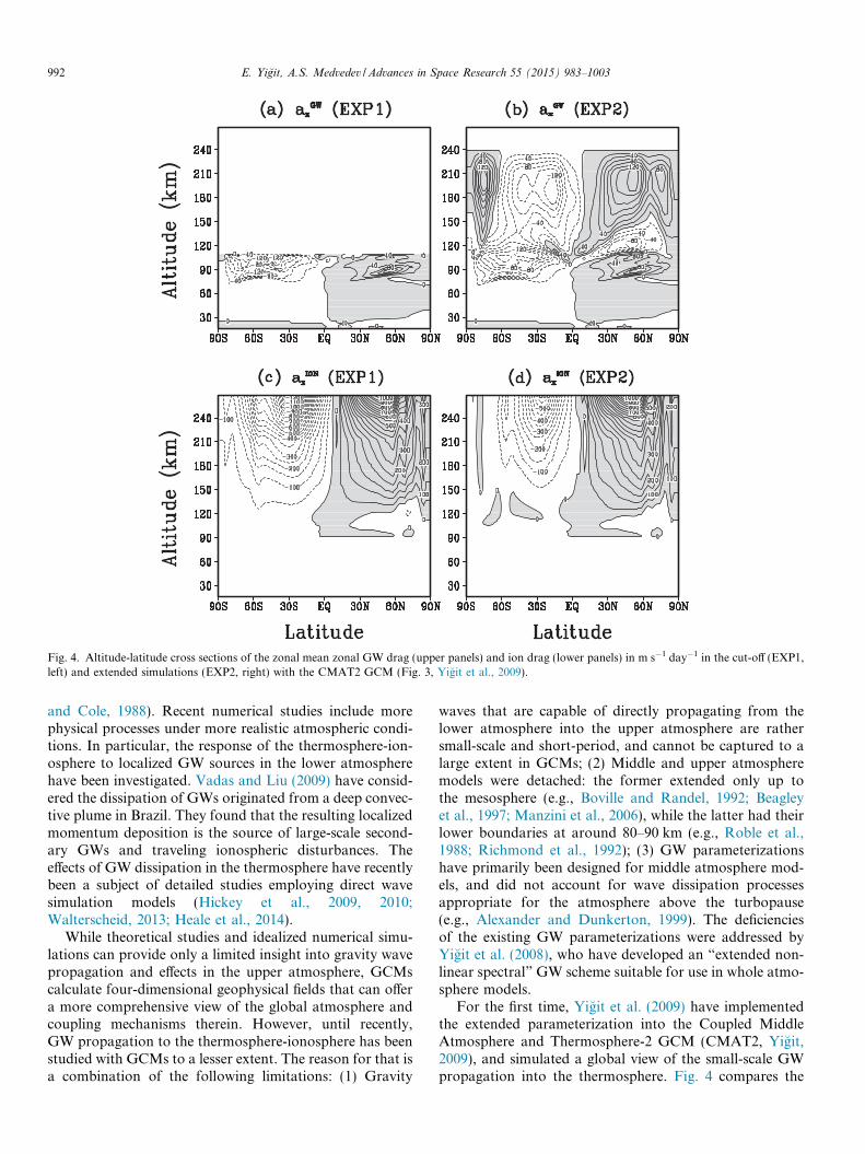
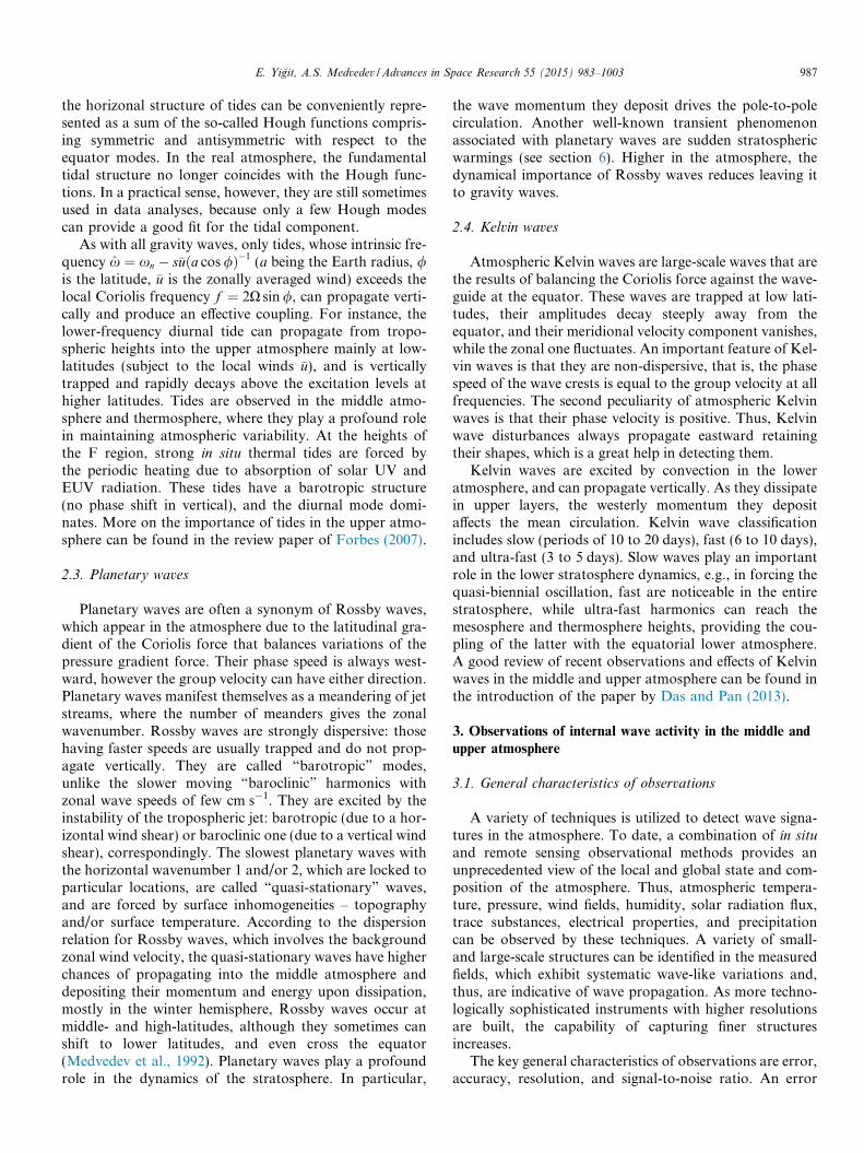
Fig. 4. Altitude-latitude cross sections of the zonal mean zonal GW drag (upper panels) and ion drag (lower panels) in m s�1 day�1 in the cut-off (EXP1,left) and extended simulations (EXP2, right) with the CMAT2 GCM (Fig. 3, Yigit et al., 2009).
992 E. Yigit, A.S. Medvedev / Advances in Space Research 55 (2015) 983–1003
and Cole, 1988). Recent numerical studies include morephysical processes under more realistic atmospheric condi-tions. In particular, the response of the thermosphere-ion-osphere to localized GW sources in the lower atmospherehave been investigated. Vadas and Liu (2009) have consid-ered the dissipation of GWs originated from a deep convec-tive plume in Brazil. They found that the resulting localizedmomentum deposition is the source of large-scale second-ary GWs and traveling ionospheric disturbances. Theeffects of GW dissipation in the thermosphere have recentlybeen a subject of detailed studies employing direct wavesimulation models (Hickey et al., 2009, 2010;Walterscheid, 2013; Heale et al., 2014).
While theoretical studies and idealized numerical simu-lations can provide only a limited insight into gravity wavepropagation and effects in the upper atmosphere, GCMscalculate four-dimensional geophysical fields that can offera more comprehensive view of the global atmosphere andcoupling mechanisms therein. However, until recently,GW propagation to the thermosphere-ionosphere has beenstudied with GCMs to a lesser extent. The reason for that isa combination of the following limitations: (1) Gravity
waves that are capable of directly propagating from thelower atmosphere into the upper atmosphere are rathersmall-scale and short-period, and cannot be captured to alarge extent in GCMs; (2) Middle and upper atmospheremodels were detached: the former extended only up tothe mesosphere (e.g., Boville and Randel, 1992; Beagleyet al., 1997; Manzini et al., 2006), while the latter had theirlower boundaries at around 80–90 km (e.g., Roble et al.,1988; Richmond et al., 1992); (3) GW parameterizationshave primarily been designed for middle atmosphere mod-els, and did not account for wave dissipation processesappropriate for the atmosphere above the turbopause(e.g., Alexander and Dunkerton, 1999). The deficienciesof the existing GW parameterizations were addressed byYigit et al. (2008), who have developed an “extended non-linear spectral” GW scheme suitable for use in whole atmo-sphere models.
For the first time, Yigit et al. (2009) have implementedthe extended parameterization into the Coupled MiddleAtmosphere and Thermosphere-2 GCM (CMAT2, Yigit,2009), and simulated a global view of the small-scale GWpropagation into the thermosphere. Fig. 4 compares the
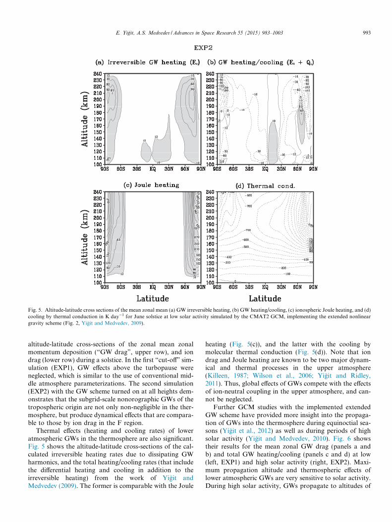
Fig. 5. Altitude-latitude cross sections of the mean zonal mean (a) GW irreversible heating, (b) GW heating/cooling, (c) ionospheric Joule heating, and (d)cooling by thermal conduction in K day�1 for June solstice at low solar activity simulated by the CMAT2 GCM, implementing the extended nonlineargravity scheme (Fig. 2, Yigit and Medvedev, 2009).
E. Yigit, A.S. Medvedev / Advances in Space Research 55 (2015) 983–1003 993
altitude-latitude cross-sections of the zonal mean zonalmomentum deposition (“GW drag”, upper row), and iondrag (lower row) during a solstice. In the first “cut-off” sim-ulation (EXP1), GW effects above the turbopause wereneglected, which is similar to the use of conventional mid-dle atmosphere parameterizations. The second simulation(EXP2) with the GW scheme turned on at all heights dem-onstrates that the subgrid-scale nonorographic GWs of thetropospheric origin are not only non-negligible in the ther-mosphere, but produce dynamical effects that are compara-ble to those by ion drag in the F region.
Thermal effects (heating and cooling rates) of loweratmospheric GWs in the thermosphere are also significant.Fig. 5 shows the altitude-latitude cross-sections of the cal-culated irreversible heating rates due to dissipating GWharmonics, and the total heating/cooling rates (that includethe differential heating and cooling in addition to theirreversible heating) from the work of Yigit andMedvedev (2009). The former is comparable with the Joule
heating (Fig. 5(c)), and the latter with the cooling bymolecular thermal conduction (Fig. 5(d)). Note that iondrag and Joule heating are known to be two major dynam-ical and thermal processes in the upper atmosphere(Killeen, 1987; Wilson et al., 2006; Yigit and Ridley,2011). Thus, global effects of GWs compete with the effectsof ion-neutral coupling in the upper atmosphere, and can-not be neglected.
Further GCM studies with the implemented extendedGW scheme have provided more insight into the propaga-tion of GWs into the thermosphere during equinoctial sea-sons (Yigit et al., 2012) as well as during periods of highsolar activity (Yigit and Medvedev, 2010). Fig. 6 showstheir results for the mean zonal GW drag (panels a andb) and total GW heating/cooling (panels c and d) at low(left, EXP1) and high solar activity (right, EXP2). Maxi-mum propagation altitude and thermospheric effects oflower atmospheric GWs are very sensitive to solar activity.During high solar activity, GWs propagate to altitudes of
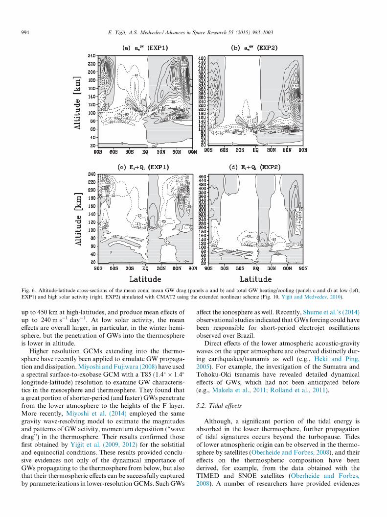
Fig. 6. Altitude-latitude cross-sections of the mean zonal mean GW drag (panels a and b) and total GW heating/cooling (panels c and d) at low (left,EXP1) and high solar activity (right, EXP2) simulated with CMAT2 using the extended nonlinear scheme (Fig. 10, Yigit and Medvedev, 2010).
994 E. Yigit, A.S. Medvedev / Advances in Space Research 55 (2015) 983–1003
up to 450 km at high-latitudes, and produce mean effects ofup to 240 m s�1 day�1. At low solar activity, the meaneffects are overall larger, in particular, in the winter hemi-sphere, but the penetration of GWs into the thermosphereis lower in altitude.
Higher resolution GCMs extending into the thermo-sphere have recently been applied to simulate GW propaga-tion and dissipation. Miyoshi and Fujiwara (2008) have useda spectral surface-to-exobase GCM with a T85 (1:4� � 1:4�
longitude-latitude) resolution to examine GW characteris-tics in the mesosphere and thermosphere. They found thata great portion of shorter-period (and faster) GWs penetratefrom the lower atmosphere to the heights of the F layer.More recently, Miyoshi et al. (2014) employed the samegravity wave-resolving model to estimate the magnitudesand patterns of GW activity, momentum deposition (“wavedrag”) in the thermosphere. Their results confirmed thosefirst obtained by Yigit et al. (2009, 2012) for the solstitialand equinoctial conditions. These results provided conclu-sive evidences not only of the dynamical importance ofGWs propagating to the thermosphere from below, but alsothat their thermospheric effects can be successfully capturedby parameterizations in lower-resolution GCMs. Such GWs
affect the ionosphere as well. Recently, Shume et al.’s (2014)observational studies indicated that GWs forcing could havebeen responsible for short-period electrojet oscillationsobserved over Brazil.
Direct effects of the lower atmospheric acoustic-gravitywaves on the upper atmosphere are observed distinctly dur-ing earthquakes/tsunamis as well (e.g., Heki and Ping,2005). For example, the investigation of the Sumatra andTohoku-Oki tsunamis have revealed detailed dynamicaleffects of GWs, which had not been anticipated before(e.g., Makela et al., 2011; Rolland et al., 2011).
5.2. Tidal effects
Although, a significant portion of the tidal energy isabsorbed in the lower thermosphere, further propagationof tidal signatures occurs beyond the turbopause. Tidesof lower atmospheric origin can be observed in the thermo-sphere by satellites (Oberheide and Forbes, 2008), and theireffects on the thermospheric composition have beenderived, for example, from the data obtained with theTIMED and SNOE satellites (Oberheide and Forbes,2008). A number of researchers have provided evidences
(a)
(b)
(c)
(d)
(e)
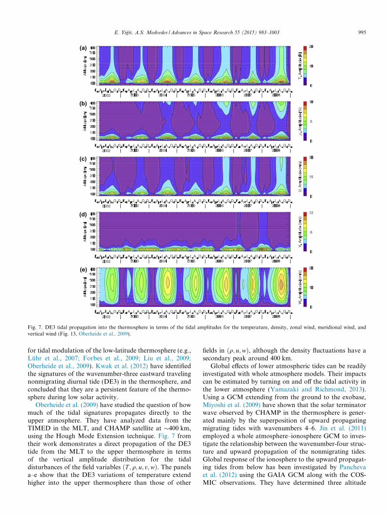
Fig. 7. DE3 tidal propagation into the thermosphere in terms of the tidal amplitudes for the temperature, density, zonal wind, meridional wind, andvertical wind (Fig. 13, Oberheide et al., 2009).
E. Yigit, A.S. Medvedev / Advances in Space Research 55 (2015) 983–1003 995
for tidal modulation of the low-latitude thermosphere (e.g.,Luhr et al., 2007; Forbes et al., 2009; Liu et al., 2009;Oberheide et al., 2009). Kwak et al. (2012) have identifiedthe signatures of the wavenumber-three eastward travelingnonmigrating diurnal tide (DE3) in the thermosphere, andconcluded that they are a persistent feature of the thermo-sphere during low solar activity.
Oberheide et al. (2009) have studied the question of howmuch of the tidal signatures propagates directly to theupper atmosphere. They have analyzed data from theTIMED in the MLT, and CHAMP satellite at �400 km,using the Hough Mode Extension technique. Fig. 7 fromtheir work demonstrates a direct propagation of the DE3tide from the MLT to the upper thermosphere in termsof the vertical amplitude distribution for the tidaldisturbances of the field variables ðT ; q; u; v;wÞ. The panelsa–e show that the DE3 variations of temperature extendhigher into the upper thermosphere than those of other
fields in ðq; u;wÞ, although the density fluctuations have asecondary peak around 400 km.
Global effects of lower atmospheric tides can be readilyinvestigated with whole atmosphere models. Their impactscan be estimated by turning on and off the tidal activity inthe lower atmosphere (Yamazaki and Richmond, 2013).Using a GCM extending from the ground to the exobase,Miyoshi et al. (2009) have shown that the solar terminatorwave observed by CHAMP in the thermosphere is gener-ated mainly by the superposition of upward propagatingmigrating tides with wavenumbers 4–6. Jin et al. (2011)employed a whole atmosphere–ionosphere GCM to inves-tigate the relationship between the wavenumber-four struc-ture and upward propagation of the nonmigrating tides.Global response of the ionosphere to the upward propagat-ing tides from below has been investigated by Panchevaet al. (2012) using the GAIA GCM along with the COS-MIC observations. They have determined three altitude
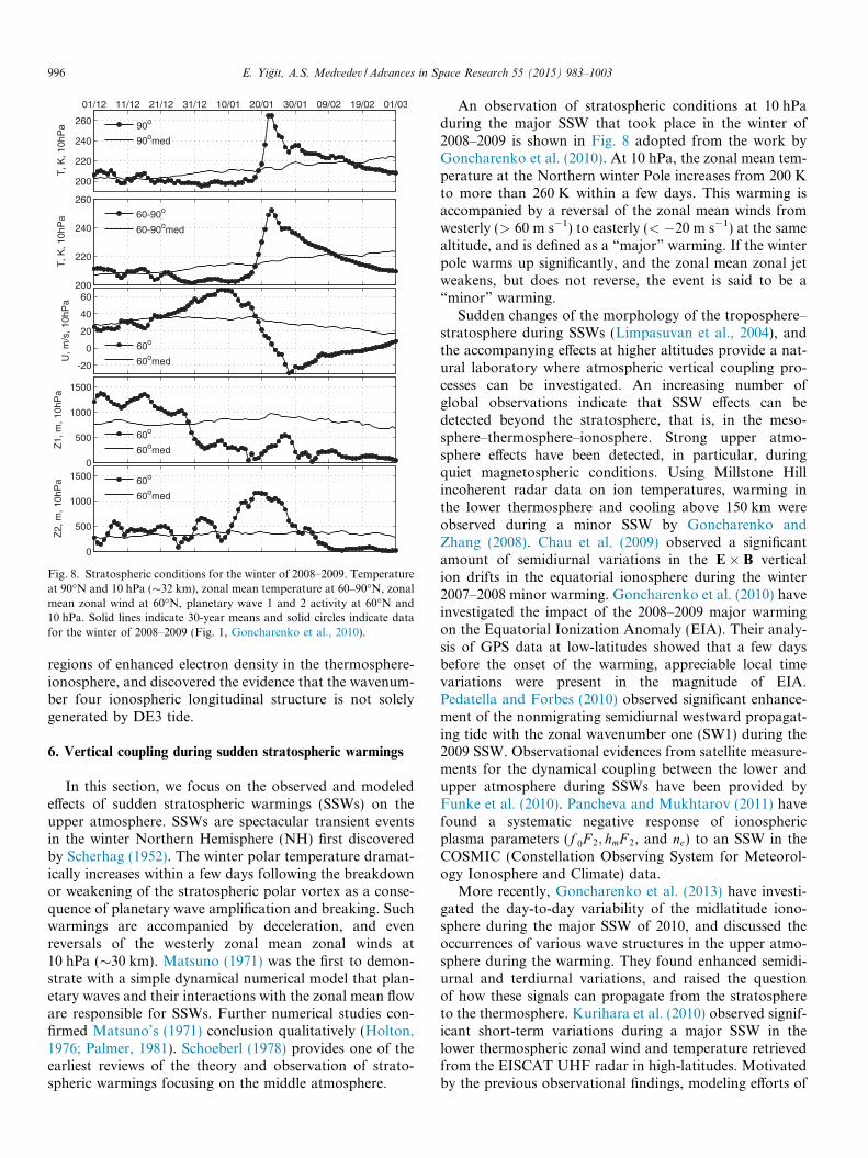
Fig. 8. Stratospheric conditions for the winter of 2008–2009. Temperatureat 90�N and 10 hPa (�32 km), zonal mean temperature at 60–90�N, zonalmean zonal wind at 60�N, planetary wave 1 and 2 activity at 60�N and10 hPa. Solid lines indicate 30-year means and solid circles indicate datafor the winter of 2008–2009 (Fig. 1, Goncharenko et al., 2010).
996 E. Yigit, A.S. Medvedev / Advances in Space Research 55 (2015) 983–1003
regions of enhanced electron density in the thermosphere-ionosphere, and discovered the evidence that the wavenum-ber four ionospheric longitudinal structure is not solelygenerated by DE3 tide.
6. Vertical coupling during sudden stratospheric warmings
In this section, we focus on the observed and modeledeffects of sudden stratospheric warmings (SSWs) on theupper atmosphere. SSWs are spectacular transient eventsin the winter Northern Hemisphere (NH) first discoveredby Scherhag (1952). The winter polar temperature dramat-ically increases within a few days following the breakdownor weakening of the stratospheric polar vortex as a conse-quence of planetary wave amplification and breaking. Suchwarmings are accompanied by deceleration, and evenreversals of the westerly zonal mean zonal winds at10 hPa (�30 km). Matsuno (1971) was the first to demon-strate with a simple dynamical numerical model that plan-etary waves and their interactions with the zonal mean floware responsible for SSWs. Further numerical studies con-firmed Matsuno’s (1971) conclusion qualitatively (Holton,1976; Palmer, 1981). Schoeberl (1978) provides one of theearliest reviews of the theory and observation of strato-spheric warmings focusing on the middle atmosphere.
An observation of stratospheric conditions at 10 hPaduring the major SSW that took place in the winter of2008–2009 is shown in Fig. 8 adopted from the work byGoncharenko et al. (2010). At 10 hPa, the zonal mean tem-perature at the Northern winter Pole increases from 200 Kto more than 260 K within a few days. This warming isaccompanied by a reversal of the zonal mean winds fromwesterly (> 60 m s�1) to easterly (< �20 m s�1) at the samealtitude, and is defined as a “major” warming. If the winterpole warms up significantly, and the zonal mean zonal jetweakens, but does not reverse, the event is said to be a“minor” warming.
Sudden changes of the morphology of the troposphere–stratosphere during SSWs (Limpasuvan et al., 2004), andthe accompanying effects at higher altitudes provide a nat-ural laboratory where atmospheric vertical coupling pro-cesses can be investigated. An increasing number ofglobal observations indicate that SSW effects can bedetected beyond the stratosphere, that is, in the meso-sphere–thermosphere–ionosphere. Strong upper atmo-sphere effects have been detected, in particular, duringquiet magnetospheric conditions. Using Millstone Hillincoherent radar data on ion temperatures, warming inthe lower thermosphere and cooling above 150 km wereobserved during a minor SSW by Goncharenko andZhang (2008). Chau et al. (2009) observed a significantamount of semidiurnal variations in the E� B verticalion drifts in the equatorial ionosphere during the winter2007–2008 minor warming. Goncharenko et al. (2010) haveinvestigated the impact of the 2008–2009 major warmingon the Equatorial Ionization Anomaly (EIA). Their analy-sis of GPS data at low-latitudes showed that a few daysbefore the onset of the warming, appreciable local timevariations were present in the magnitude of EIA.Pedatella and Forbes (2010) observed significant enhance-ment of the nonmigrating semidiurnal westward propagat-ing tide with the zonal wavenumber one (SW1) during the2009 SSW. Observational evidences from satellite measure-ments for the dynamical coupling between the lower andupper atmosphere during SSWs have been provided byFunke et al. (2010). Pancheva and Mukhtarov (2011) havefound a systematic negative response of ionosphericplasma parameters (f 0F 2; hmF 2, and ne) to an SSW in theCOSMIC (Constellation Observing System for Meteorol-ogy Ionosphere and Climate) data.
More recently, Goncharenko et al. (2013) have investi-gated the day-to-day variability of the midlatitude iono-sphere during the major SSW of 2010, and discussed theoccurrences of various wave structures in the upper atmo-sphere during the warming. They found enhanced semidi-urnal and terdiurnal variations, and raised the questionof how these signals can propagate from the stratosphereto the thermosphere. Kurihara et al. (2010) observed signif-icant short-term variations during a major SSW in thelower thermospheric zonal wind and temperature retrievedfrom the EISCAT UHF radar in high-latitudes. Motivatedby the previous observational findings, modeling efforts of
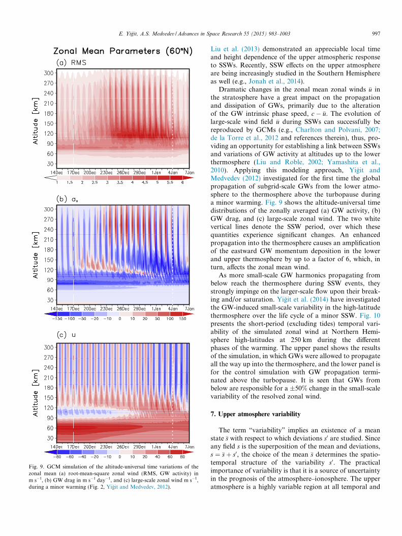
Fig. 9. GCM simulation of the altitude-universal time variations of thezonal mean (a) root-mean-square zonal wind (RMS, GW activity) inm s�1, (b) GW drag in m s�1 day�1, and (c) large-scale zonal wind m s�1,during a minor warming (Fig. 2, Yigit and Medvedev, 2012).
E. Yigit, A.S. Medvedev / Advances in Space Research 55 (2015) 983–1003 997
Liu et al. (2013) demonstrated an appreciable local timeand height dependence of the upper atmospheric responseto SSWs. Recently, SSW effects on the upper atmosphereare being increasingly studied in the Southern Hemisphereas well (e.g., Jonah et al., 2014).
Dramatic changes in the zonal mean zonal winds �u inthe stratosphere have a great impact on the propagationand dissipation of GWs, primarily due to the alterationof the GW intrinsic phase speed, c� �u. The evolution oflarge-scale wind field �u during SSWs can successfully bereproduced by GCMs (e.g., Charlton and Polvani, 2007;de la Torre et al., 2012 and references therein), thus, pro-viding an opportunity for establishing a link between SSWsand variations of GW activity at altitudes up to the lowerthermosphere (Liu and Roble, 2002; Yamashita et al.,2010). Applying this modeling approach, Yigit andMedvedev (2012) investigated for the first time the globalpropagation of subgrid-scale GWs from the lower atmo-sphere to the thermosphere above the turbopause duringa minor warming. Fig. 9 shows the altitude-universal timedistributions of the zonally averaged (a) GW activity, (b)GW drag, and (c) large-scale zonal wind. The two whitevertical lines denote the SSW period, over which thesequantities experience significant changes. An enhancedpropagation into the thermosphere causes an amplificationof the eastward GW momentum deposition in the lowerand upper thermosphere by up to a factor of 6, which, inturn, affects the zonal mean wind.
As more small-scale GW harmonics propagating frombelow reach the thermosphere during SSW events, theystrongly impinge on the larger-scale flow upon their break-ing and/or saturation. Yigit et al. (2014) have investigatedthe GW-induced small-scale variability in the high-latitudethermosphere over the life cycle of a minor SSW. Fig. 10presents the short-period (excluding tides) temporal vari-ability of the simulated zonal wind at Northern Hemi-sphere high-latitudes at 250 km during the differentphases of the warming. The upper panel shows the resultsof the simulation, in which GWs were allowed to propagateall the way up into the thermosphere, and the lower panel isfor the control simulation with GW propagation termi-nated above the turbopause. It is seen that GWs frombelow are responsible for a �50% change in the small-scalevariability of the resolved zonal wind.
7. Upper atmosphere variability
The term “variability” implies an existence of a meanstate �s with respect to which deviations s0 are studied. Sinceany field s is the superposition of the mean and deviations,s ¼ �sþ s0, the choice of the mean �s determines the spatio-temporal structure of the variability s0. The practicalimportance of variability is that it is a source of uncertaintyin the prognosis of the atmosphere–ionosphere. The upperatmosphere is a highly variable region at all temporal and
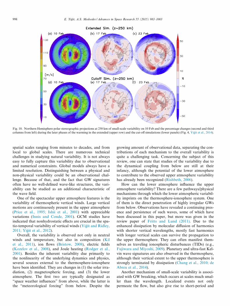
Fig. 10. Northern Hemisphere polar stereographic projections at 250 km of small-scale variability on 10 Feb and the percentage changes (second and thirdcolumns from left) during the later phases of the warming in the extended (upper row) and the cut-off simulations (lower panels) (Fig. 4, Yigit et al., 2014).
998 E. Yigit, A.S. Medvedev / Advances in Space Research 55 (2015) 983–1003
spatial scales ranging from minutes to decades, and fromlocal to global scales. There are numerous technicalchallenges in studying natural variability. It is not alwayseasy to fully capture this variability due to observationaland numerical constraints. Global models always have alimited resolution. Distinguishing between a physical andnon-physical variability could be an observational chal-lenge. Because of that, and the fact that GW signaturesoften have no well-defined wave-like structures, the vari-ability can be studied as an additional characteristic ofthe wave field.
One of the spectacular upper atmosphere features is thevariability of thermospheric vertical winds. Large verticalmotions are continuously present in the upper atmosphere(Price et al., 1995; Ishii et al., 2001) with appreciablevariations (Innis and Conde, 2001). GCM studies haveindicated that nonhydrostatic effects are crucial in the spa-tio-temporal variability of vertical winds (Yigit and Ridley,2011; Yigit et al., 2012).
Overall, the variability is observed not only in neutralwinds and temperature, but also in composition (Kilet al., 2011), ion flows (Bristow, 2008), electric fields(Kozelov et al., 2008), and Joule heating (Rodger et al.,2001). Besides the inherent variability due primarily tothe nonlinearity of the underlying dynamics and physics,several sources external to the thermosphere-ionospherehave been identified. They are changes in (1) the solar irra-diation, (2) magnetospheric forcing, and (3) the loweratmosphere. The first two are typically designated as“space weather influences” from above, while the latter isthe “meteorological forcing” from below. Despite the
growing amount of observational data, separating the con-tributions of each mechanism to the overall variability isquite a challenging task. Concerning the subject of thisreview, one can state that studies of the variability due tothe dynamical coupling from below are still at theirinfancy, although the potential of the lower atmosphereto contribute to the observed upper atmosphere variabilityhas already been recognized (Rishbeth, 2006).
How can the lower atmosphere influence the upperatmosphere variability? There are a few pathways/physicalmechanisms through which the lower atmospheric variabil-ity imprints on the thermosphere-ionosphere system. Oneof them is the direct penetration of highly irregular GWsfrom below. Observations have revealed a continuing pres-ence and persistence of such waves, some of which havebeen discussed in this paper, but more was given in thereview paper of Fritts and Lund (2011). Due to theenhanced dissipation by molecular diffusion of harmonicswith shorter vertical wavelengths, mostly fast harmonicswith longer vertical scales can survive the propagation tothe upper thermosphere. They can often manifest them-selves as traveling ionospheric disturbances (TIDs) (e.g.,Fujiwara and Miyoshi, 2009). Planetary and ultra-fast Kel-vin wave signatures are also observed in the thermosphere,although their vertical extent to the upper thermosphere isstrongly terminated by dissipation (Chang et al., 2010; deAbreu et al., 2014).
Another mechanism of small-scale variability is associ-ated with GW breaking, which occurs at scales much smal-ler than the wavelength. Localized events not onlypermeate the flow, but also give rise to short-period and
E. Yigit, A.S. Medvedev / Advances in Space Research 55 (2015) 983–1003 999
long (fast) waves. Such mechanism of secondary excitationhas been extensively studied (e.g., Vadas et al., 2003; Chunand Kim, 2008), and found to be a likely source of harmon-ics that can effectively propagate into the upper thermo-sphere (Vadas and Liu, 2011). Modulation of gravitywave propagation in the middle atmosphere, e.g., duringsudden stratospheric events (Yigit et al., 2014), or byenhanced dissipation during periods of increased solaractivity (Yigit and Medvedev, 2010) can influence theupper atmosphere variability. GWs can influence thedegree of ion-neutral coupling primarily by modulatingion-neutral differential velocities. Depending on the degreeof GW penetration into the thermosphere and the plasmaflow patterns, such modulation can constitute a significantsource of variability (Yigit et al., 2014).
The third pathway does not require a direct wave prop-agation to the upper atmosphere, but involves a chain ofadditional physical mechanisms to imprint lower atmo-spheric inhomogeneities onto the upper layers. A notableexample is the wavenumber-four longitudinal structure ofthe low-latitude ionosphere seen in electron density andtemperature, nitric oxide density, and F-region neutralwinds (see Ren et al., 2010 for more observational evi-dences). It was suggested in the work by Immel et al.(2006) that the nonmigrating diurnal tide with the wave-number-three traveling eastward is the main source of thewavenumber-four structure. The DE3 tide is generated bythe latent heat release in the tropical lower atmosphere,propagates to the MLT heights, where it reaches significantamplitudes, and can be a dominant mode of the diurnaltide during certain times (Oberheide et al., 2011). Immelet al. (2006) suggested that the DE3 tide modulates the ion-ospheric dynamo at the E-region, thus affecting electricfields in the F-region along magnetic lines, and drives theionospheric wavenumber-four structure. GCM simulations(Hagan et al., 2007) have confirmed this mechanism, whilethe subsequent studies investigated its various aspects (Renet al., 2010).
8. Open questions and concluding remarks
A concise review of vertical coupling in the atmosphere–ionosphere system has been presented here, focusing on therole of internal waves as the main vertical coupling mech-anism. Considerable progress has been made, over the pastdecade, in the appreciation of the role, which these wavesplay in the dynamical coupling between the lower andupper atmosphere. Internal waves include planetary Ross-by and Kelvin waves, tides, and gravity waves. Due to theirability to propagate vertically, internal waves represent adynamical link between atmospheric layers.
There are many open questions that still remain in thisresearch area, some of which are listed below. We do notintend to compile a full list of them, but name the mostbasic and pressing, in our view, unresolved problems.
1. What are the momentum fluxes and spectra of internalgravity waves penetrating into the thermosphere frombelow?
2. Can the sources of gravity waves be parameterized interms of large-scale fields, such that the generation canbe modeled by GCMs self-consistently, rather thanintroduced as external tuning parameters?
3. To what degree do the external energy sources (solarirradiation, geomagnetic activity) and the associatedvariability in the upper atmosphere affect the middle,and even lower atmosphere? What are the dynamicalmechanisms?
4. What information from the lower atmosphere is neededto predict the dynamical variability above?
Although the focus of this review has been on the Earthatmosphere, internal wave coupling has wider implications,for instance, for understanding circulations of other plan-ets, like Mars (Medvedev et al., 2011, Medvedev andYigit, 2012), and Venus (Garcia et al., 2009), as well.
Acknowledgments
The work was partially supported by German ScienceFoundation (DFG) Grant ME2752/3-1. Erdal Yigit waspartially supported by NASA – United States GrantNNX13AO36G. The authors are grateful to Art Polandat George Mason University’s Space Weather Laboratoryfor his valuable comments on the manuscript.
References
Abdu, M.A., Kherani, E.A., Batista, I.S., de Paula, E.R., Fritts, D.C.,Sobral, J.H.A., 2009. Gravity wave initiation of equatorial spread F/plasma bubble irregularities based on observational data from theSpreadFEx campaign. Ann. Geophys. 27, 2607–2622.
Alexander, M.J., Dunkerton, T.J., 1999. A spectral parameterization ofmean-flow forcing due to breaking gravity waves. J. Atmos. Sci. 56,4167–4182.
Altadill, D., Apostolov, E.M., Boska, J., Lastovicka, J., 2004. Planetaryand gravity wave signatures in the F-region ionosphere with impact onradio propagation predictions and variability. Ann. Geophys. 47,1109–1119.
Beagley, S.R., de Grandepre, J., Koshyk, J.N., McFarlane, N.A.,Shepherd, T.G., 1997. Radiative-dynamical climatology of the firstgeneration Canadian middle atmosphere model. Atmos. Ocean 35,293–331.
Becker, E., 2004. Direct heating rates associated with gravity wavesaturation. J. Atmos. Sol.-Terr. Phys. 66, 683–696.
Becker, E., 2011. Dynamical control of the middle atmosphere. Space Sci.Rev. 168, 283–314. http://dx.doi.org/10.1007/s11214-011-9841-5.
Bilitza, D., Altadill, D., Zhang, Y., Mertens, C., Truhlik, V., et al., 2014.The international reference ionosphere 2012 – a model of internationalcollaboration. J. Space Weather Space Clim. 4, A07.
Boville, B.A., Randel, W.J., 1992. Equatorial waves in a stratosphericgcm: effects of vertical resolution. J. Atmos. Sci. 49, 785–801.
Bristow, W., 2008. Statistics of velocity fluctuations observed by Super-DARN under steady interplanetary magnetic field conditions. J.Geophys. Res. 113, A11202. http://dx.doi.org/10.1029/2008JA013203.
Chang, L.C., Palo, S.E., Liu, H., Fang, T., Lin, C.S., 2010. Response ofthe thermosphere and ionosphere to an ultra fast kelvin wave. J.
1000 E. Yigit, A.S. Medvedev / Advances in Space Research 55 (2015) 983–1003
Geophys. Res. 115, A00G04. http://dx.doi.org/10.1029/2010JA015453.
Charlton, A.J., Polvani, M.L., 2007. A new look at stratospheric suddenwarmings. Part i: Climatology and modeling benchmarks. J. Clim. 20.http://dx.doi.org/10.1175/JCLI3996.1.
Chau, J.L., Fejer, B.G., Goncharenko, L.P., 2009. Quiet variability ofequatorial E � B drifts during a sudden stratospheric warming event.Geophys. Res. Lett. 36, L05101. http://dx.doi.org/10.1029/2008GL036785.
Chun, H.-Y., Kim, Y.-H., 2008. Secondary waves generated by breakingof convective gravity waves in the mesosphere and their influence in thewave momentum flux. J. Geophys. Res. 113, D23107. http://dx.doi.org/10.1029/2008JD009792.
Curry, M.J., Murty, R.C., 1973. Thunderstorm-generated gravity waves.J. Atmos. Sci. 31, 1402–1408.
Das, U., Pan, C.J., 2013. Strong kelvin wave activity observed during thewesterly phase of QBO – a case study. Ann. Geophys. 31, 581–590.http://dx.doi.org/10.5194/angeo-31-581-2013.
de Abreu, A.J., Fagundes, P.R., Bolzan, M.J.A., Gende, M., Brunini, C.,de Jesus, R., Pillat, V.G., Abalde, J.R., Lima, W.L.C., 2014. Travelingplanetary wave ionospheric disturbances and their role in the gener-ation of equatorial Spread-F and GPS phase fluctuations during thelast extreme low solar activity and comparison with high solar activity.J. Atmos. Sol.-Terr. Phys. 117, 7–19.
de la Torre, L., Garcia, R.R., Barriopedro, D., Chandran, A., 2012.Climatology and characteristics of stratospheric sudden warmings inthe whole atmosphere community climate model. J. Geophys. Res.117. http://dx.doi.org/10.1029/2011JD016840.
Djuth, F.T., Sulzer, M.P., Gonzales, S.A., Mathews, J.D., Elder, J.H.,Walterscheid, R.L., 2004. A continuum of gravity waves in the Arecibothermosphere? J. Geophys. Res. 31, L16801. http://dx.doi.org/10.1029/2003GL019376.
Ern, M., Preusse, P., Alexander, M.J., Warner, C.D., 2004. Absolutevalues of gravity wave momentum flux derived from satellite data. J.Geophys. Res. 109, D20103. http://dx.doi.org/10.1029/2004JD004752.
Ern, M., Arras, C., Frohlich, A.F.K., Jacobi, C., Kalisch, S., Krebsbach,M., Preusse, P., Schmidt, T., Wickert, J., 2013. Observations and raytracing of gravity waves: Implications for global modeling. In: Lubken,F.-J. (Ed.), Climate and Weather of the Sun–Earth System (CAW-SES), Springer Atmospheric Sciences. Springer, Netherlands, pp. 383–408. http://dx.doi.org/10.1007/978-94-007-4348-921.
Evan, S., Alexander, M.J., Dudhia, J., 2012. Model study of intermediate-scale tropical inertia-gravity waves and comparison to TWP-ICEcampaign. J. Atmos. Sci. 69, 591–610. http://dx.doi.org/10.1175/JAS-D-11-051.1.
Forbes, J.M., 2007. Dynamics of the upper mesosphere and thermosphere.J. Meteor. Soc. Jpn. 85B, 193–213.
Forbes, J.M., Bruinsma, S.L., Zhang, X., Oberheide, J., 2009. Surface-exosphere coupling due to thermal tides. Geophys. Res. Lett. 36.http://dx.doi.org/10.1029/2009GL038748.
Frey, H.U., Mende, S.B., Arens, J.F., McCullough, P.R., Swenso, G.R.,2000. Atmospheric gravity wave signatures in the infrared hydroxyl ohairglow. Geophys. Res. Lett. 27 (1), 41–44.
Fritts, D.C., Alexander, M.J., 2003. Gravity wave dynamics and effects inthe middle atmosphere. Rev. Geophys. 41 (1), 1003. http://dx.doi.org/10.1029/2001RG000106.
Fritts, D.C., Lund, T.C., 2011. Gravity wave influences in the thermo-sphere and ionosphere: Observations and recent modeling. In: Aeron-omy of the Earth’s Atmosphere and Ionosphere. IAGA SpecialSopron Book Series. Springer, Netherlands, pp. 109–130. http://dx.doi.org/10.1007/978-94-007-0326-18.
Fritts, D.C., Wang, L., Werne, J., Lund, T., Wan, K., 2009. Gravity waveinstability dynamics at high Reynolds numbers. Part I: Wave fieldevolution at large amplitudes and high frequencies. J. Atmos. Sci. 66,1126–1148. http://dx.doi.org/10.1175/2008JAS2726.1.
Fritts, D.C., Janches, D., Iimura, H., Hocking, W.K., Mitchell, N.J.,Stockwell, R.G., Fuller, B., Vandepeer, B., Hormaechea, J., Brunini,C., Levato, H., 2010. Southern Argentina agile meteor radar: system
design and initial measurements of large-scale winds and tides. J.Geophys. Res. 115. http://dx.doi.org/10.1029/2010JD013850.
Fujiwara, H., Miyoshi, Y., 2009. Global distribution of the thermosphericdisturbances produced by effects from the upper and lower regions:simulations by a whole atmosphere GCM. Earth Planets Space 61,463–470.
Funke, B., Lopez-Puertas, M., Bermejo-Pantalen, D., Garca-Comas, M.,Stiller, G.P., von Clarmann, T., Kiefer, M., Linden, A., 2010. Evidencefor dynamical coupling from the lower atmosphere to the thermo-sphere during a major stratospheric warming. Geophys. Res. Lett. 37(13). http://dx.doi.org/10.1029/2010GL043619.
Gall, R.L., Williams, R.T., Clark, T.L., 1988. Gravity waves generatedduring frontogenesis. J. Atmos. Sci. 45, 2204–2219.
Gardner, L.C., Schunk, R.W., 2011. Large-scale gravity wave character-istics simulated with a high-resolution global thermosphere–iono-sphere model. J. Geophys. Res. 116, A06303. http://dx.doi.org/10.1029/2010JA015629.
Garcia, R.F., Drossart, P., Piccioni, G., Lopez-Valverde, M., Occhipinti,G., 2009. Gravity waves in the upper atmosphere of Venus revealed byCO2 nonlocal thermodynamic equilibrium emissions. J. Geophys. Res.114. http://dx.doi.org/10.1029/2008JE003073.
Gavrilov, N.M., Kshevtskii, S.P., 2013. Numerical modeling of propaga-tion of breaking nonlinear acoustic-gravity waves from the lower to theupper atmosphere. Adv. Space Res. 51, 1168–1174. http://dx.doi.org/10.1016/j.asr.2012.10.023.
Goncharenko, L., Zhang, S.-R., 2008. Ionospheric signatures of suddenstratospheric warming: ion temperature at middle latitude. Geophys.Res. Lett. 35, L21103. http://dx.doi.org/10.1029/2008GL035684.
Goncharenko, L.P., Coster, A.J., Chau, J.L., Valladares, C.E., 2010.Impact of sudden stratospheric warmings on equatorial ionizationanomaly. J. Geophys. Res. 115, A00G07. http://dx.doi.org/10.1029/2010JA015400.
Goncharenko, L.P., Hsu, V.W., Brum, C.G.M., Zhang, S.-R., Fentzke,J.T., 2013. Wave signatures in the midlatitude ionosphere during asudden stratospheric warming of january 2010. J. Geophys. Res. SpacePhys 118. http://dx.doi.org/10.1029/2012JA018251.
Hagan, M.E., Forbes, J.M., 2002. Migrating and nonmigrating diurnaltides in the middle and upper atmosphere excited by troposphericlatent heat release. J. Geophys. Res. 107 (D24), 4754. http://dx.doi.org/10.1029/2001JD001236.
Hagan, M.E., Maute, A., Roble, R.G., Richmond, A.D., Immel, T.J.,England, S.L., 2007. Connections between deep tropical clouds and theEarth’s ionosphere. Geophys. Res. Lett. 34, L20109. http://dx.doi.org/10.1029/2007GL030142.
Heale, C.J., Snively, J.B., Hickey, M.P., Ali, C.J., 2014. Thermosphericdissipation of upward propagating gravity wave packets. J. Geophys.Res. Space Phys. 119, 3857–3872. http://dx.doi.org/10.1002/2013JA019387.
Heki, K., Ping, J., 2005. Directivity and apparent velocity of the coseismicionospheric disturbances observed with a dense GPS array. EarthPlanet. Sci. Lett. 236, 845–855.
Hickey, M.P., Cole, K.D., 1988. A numerical model for gravity wavedissipation in the thermosphere. J. Atmos. Terr. Phys. 50, 689–697.
Hickey, M.P., Schubert, G., Walterscheid, R.L., 1993. Gravity wave-driven fluctuations in the O2 atmospheric (0–1) nightglow from anextended, dissipative emission region. J. Geophys. Res. 98, 13717–13729.
Hickey, M.P., Schubert, G., Walterscheid, R.L., 2009. Propagation oftsunami-driven gravity waves into the thermosphere and ionosphere. J.Geophys. Res. http://dx.doi.org/10.1029/2009JA014105.
Hickey, M.P., Walterscheid, R.L., Schubert, G., 2010. Wave mean flowinteractions in the thermosphere induced by a major tsunami. J.Geophys. Res. Space Phys. 115 (A9). http://dx.doi.org/10.1029/2009JA014927.
Hoffmann, L., Xue, X., Alexander, M.J., 2013. A global view ofstratospheric gravity wave hotspots located with atmospheric infraredsounder observations. J. Geophys. Res. 118. http://dx.doi.org/10.1029/2012JD018658.
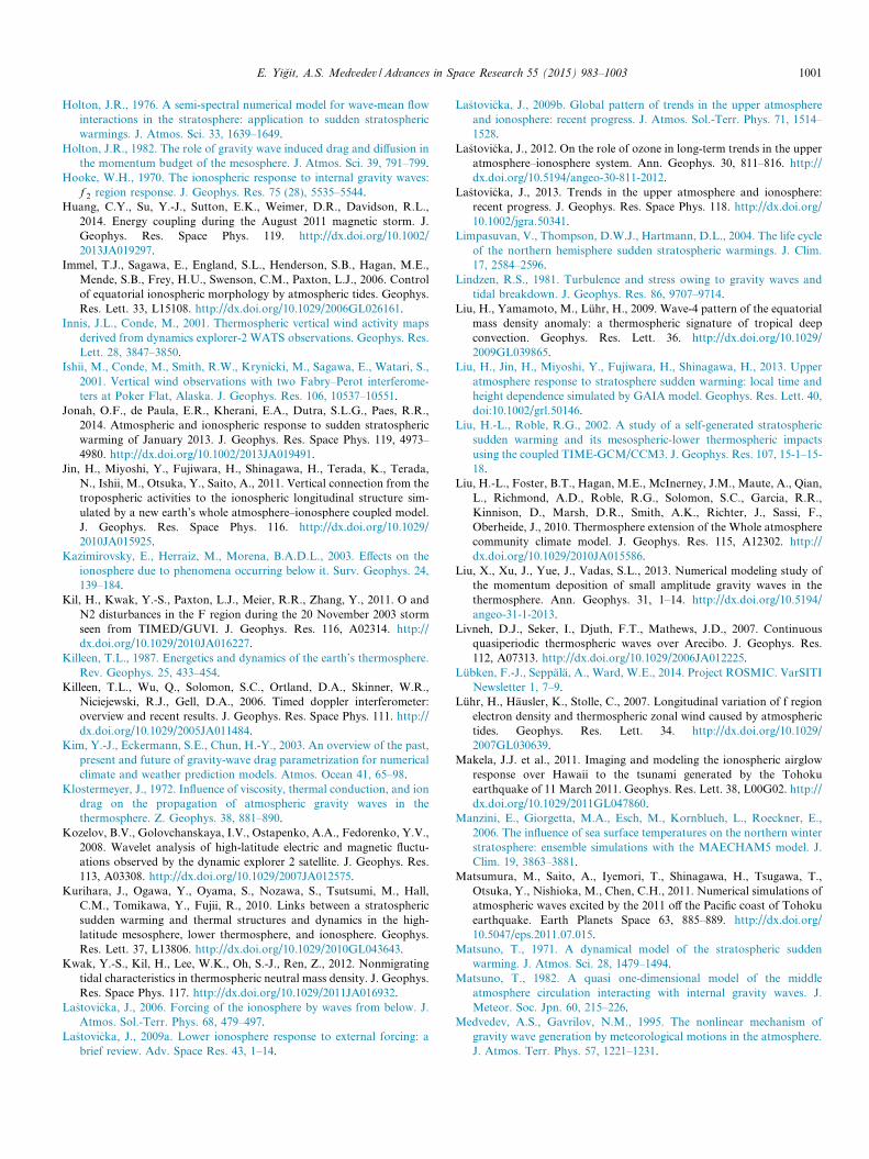
E. Yigit, A.S. Medvedev / Advances in Space Research 55 (2015) 983–1003 1001
Holton, J.R., 1976. A semi-spectral numerical model for wave-mean flowinteractions in the stratosphere: application to sudden stratosphericwarmings. J. Atmos. Sci. 33, 1639–1649.
Holton, J.R., 1982. The role of gravity wave induced drag and diffusion inthe momentum budget of the mesosphere. J. Atmos. Sci. 39, 791–799.
Hooke, W.H., 1970. The ionospheric response to internal gravity waves:f 2 region response. J. Geophys. Res. 75 (28), 5535–5544.
Huang, C.Y., Su, Y.-J., Sutton, E.K., Weimer, D.R., Davidson, R.L.,2014. Energy coupling during the August 2011 magnetic storm. J.Geophys. Res. Space Phys. 119. http://dx.doi.org/10.1002/2013JA019297.
Immel, T.J., Sagawa, E., England, S.L., Henderson, S.B., Hagan, M.E.,Mende, S.B., Frey, H.U., Swenson, C.M., Paxton, L.J., 2006. Controlof equatorial ionospheric morphology by atmospheric tides. Geophys.Res. Lett. 33, L15108. http://dx.doi.org/10.1029/2006GL026161.
Innis, J.L., Conde, M., 2001. Thermospheric vertical wind activity mapsderived from dynamics explorer-2 WATS observations. Geophys. Res.Lett. 28, 3847–3850.
Ishii, M., Conde, M., Smith, R.W., Krynicki, M., Sagawa, E., Watari, S.,2001. Vertical wind observations with two Fabry–Perot interferome-ters at Poker Flat, Alaska. J. Geophys. Res. 106, 10537–10551.
Jonah, O.F., de Paula, E.R., Kherani, E.A., Dutra, S.L.G., Paes, R.R.,2014. Atmospheric and ionospheric response to sudden stratosphericwarming of January 2013. J. Geophys. Res. Space Phys. 119, 4973–4980. http://dx.doi.org/10.1002/2013JA019491.
Jin, H., Miyoshi, Y., Fujiwara, H., Shinagawa, H., Terada, K., Terada,N., Ishii, M., Otsuka, Y., Saito, A., 2011. Vertical connection from thetropospheric activities to the ionospheric longitudinal structure sim-ulated by a new earth’s whole atmosphere–ionosphere coupled model.J. Geophys. Res. Space Phys. 116. http://dx.doi.org/10.1029/2010JA015925.
Kazimirovsky, E., Herraiz, M., Morena, B.A.D.L., 2003. Effects on theionosphere due to phenomena occurring below it. Surv. Geophys. 24,139–184.
Kil, H., Kwak, Y.-S., Paxton, L.J., Meier, R.R., Zhang, Y., 2011. O andN2 disturbances in the F region during the 20 November 2003 stormseen from TIMED/GUVI. J. Geophys. Res. 116, A02314. http://dx.doi.org/10.1029/2010JA016227.
Killeen, T.L., 1987. Energetics and dynamics of the earth’s thermosphere.Rev. Geophys. 25, 433–454.
Killeen, T.L., Wu, Q., Solomon, S.C., Ortland, D.A., Skinner, W.R.,Niciejewski, R.J., Gell, D.A., 2006. Timed doppler interferometer:overview and recent results. J. Geophys. Res. Space Phys. 111. http://dx.doi.org/10.1029/2005JA011484.
Kim, Y.-J., Eckermann, S.E., Chun, H.-Y., 2003. An overview of the past,present and future of gravity-wave drag parametrization for numericalclimate and weather prediction models. Atmos. Ocean 41, 65–98.
Klostermeyer, J., 1972. Influence of viscosity, thermal conduction, and iondrag on the propagation of atmospheric gravity waves in thethermosphere. Z. Geophys. 38, 881–890.
Kozelov, B.V., Golovchanskaya, I.V., Ostapenko, A.A., Fedorenko, Y.V.,2008. Wavelet analysis of high-latitude electric and magnetic fluctu-ations observed by the dynamic explorer 2 satellite. J. Geophys. Res.113, A03308. http://dx.doi.org/10.1029/2007JA012575.
Kurihara, J., Ogawa, Y., Oyama, S., Nozawa, S., Tsutsumi, M., Hall,C.M., Tomikawa, Y., Fujii, R., 2010. Links between a stratosphericsudden warming and thermal structures and dynamics in the high-latitude mesosphere, lower thermosphere, and ionosphere. Geophys.Res. Lett. 37, L13806. http://dx.doi.org/10.1029/2010GL043643.
Kwak, Y.-S., Kil, H., Lee, W.K., Oh, S.-J., Ren, Z., 2012. Nonmigratingtidal characteristics in thermospheric neutral mass density. J. Geophys.Res. Space Phys. 117. http://dx.doi.org/10.1029/2011JA016932.
Lastovicka, J., 2006. Forcing of the ionosphere by waves from below. J.Atmos. Sol.-Terr. Phys. 68, 479–497.
Lastovicka, J., 2009a. Lower ionosphere response to external forcing: abrief review. Adv. Space Res. 43, 1–14.
Lastovicka, J., 2009b. Global pattern of trends in the upper atmosphereand ionosphere: recent progress. J. Atmos. Sol.-Terr. Phys. 71, 1514–1528.
Lastovicka, J., 2012. On the role of ozone in long-term trends in the upperatmosphere–ionosphere system. Ann. Geophys. 30, 811–816. http://dx.doi.org/10.5194/angeo-30-811-2012.
Lastovicka, J., 2013. Trends in the upper atmosphere and ionosphere:recent progress. J. Geophys. Res. Space Phys. 118. http://dx.doi.org/10.1002/jgra.50341.
Limpasuvan, V., Thompson, D.W.J., Hartmann, D.L., 2004. The life cycleof the northern hemisphere sudden stratospheric warmings. J. Clim.17, 2584–2596.
Lindzen, R.S., 1981. Turbulence and stress owing to gravity waves andtidal breakdown. J. Geophys. Res. 86, 9707–9714.
Liu, H., Yamamoto, M., Luhr, H., 2009. Wave-4 pattern of the equatorialmass density anomaly: a thermospheric signature of tropical deepconvection. Geophys. Res. Lett. 36. http://dx.doi.org/10.1029/2009GL039865.
Liu, H., Jin, H., Miyoshi, Y., Fujiwara, H., Shinagawa, H., 2013. Upperatmosphere response to stratosphere sudden warming: local time andheight dependence simulated by GAIA model. Geophys. Res. Lett. 40,doi:10.1002/grl.50146.
Liu, H.-L., Roble, R.G., 2002. A study of a self-generated stratosphericsudden warming and its mesospheric-lower thermospheric impactsusing the coupled TIME-GCM/CCM3. J. Geophys. Res. 107, 15-1–15-18.
Liu, H.-L., Foster, B.T., Hagan, M.E., McInerney, J.M., Maute, A., Qian,L., Richmond, A.D., Roble, R.G., Solomon, S.C., Garcia, R.R.,Kinnison, D., Marsh, D.R., Smith, A.K., Richter, J., Sassi, F.,Oberheide, J., 2010. Thermosphere extension of the Whole atmospherecommunity climate model. J. Geophys. Res. 115, A12302. http://dx.doi.org/10.1029/2010JA015586.
Liu, X., Xu, J., Yue, J., Vadas, S.L., 2013. Numerical modeling study ofthe momentum deposition of small amplitude gravity waves in thethermosphere. Ann. Geophys. 31, 1–14. http://dx.doi.org/10.5194/angeo-31-1-2013.
Livneh, D.J., Seker, I., Djuth, F.T., Mathews, J.D., 2007. Continuousquasiperiodic thermospheric waves over Arecibo. J. Geophys. Res.112, A07313. http://dx.doi.org/10.1029/2006JA012225.
Lubken, F.-J., Seppala, A., Ward, W.E., 2014. Project ROSMIC. VarSITINewsletter 1, 7–9.
Luhr, H., Hausler, K., Stolle, C., 2007. Longitudinal variation of f regionelectron density and thermospheric zonal wind caused by atmospherictides. Geophys. Res. Lett. 34. http://dx.doi.org/10.1029/2007GL030639.
Makela, J.J. et al., 2011. Imaging and modeling the ionospheric airglowresponse over Hawaii to the tsunami generated by the Tohokuearthquake of 11 March 2011. Geophys. Res. Lett. 38, L00G02. http://dx.doi.org/10.1029/2011GL047860.
Manzini, E., Giorgetta, M.A., Esch, M., Kornblueh, L., Roeckner, E.,2006. The influence of sea surface temperatures on the northern winterstratosphere: ensemble simulations with the MAECHAM5 model. J.Clim. 19, 3863–3881.
Matsumura, M., Saito, A., Iyemori, T., Shinagawa, H., Tsugawa, T.,Otsuka, Y., Nishioka, M., Chen, C.H., 2011. Numerical simulations ofatmospheric waves excited by the 2011 off the Pacific coast of Tohokuearthquake. Earth Planets Space 63, 885–889. http://dx.doi.org/10.5047/eps.2011.07.015.
Matsuno, T., 1971. A dynamical model of the stratospheric suddenwarming. J. Atmos. Sci. 28, 1479–1494.
Matsuno, T., 1982. A quasi one-dimensional model of the middleatmosphere circulation interacting with internal gravity waves. J.Meteor. Soc. Jpn. 60, 215–226.
Medvedev, A.S., Gavrilov, N.M., 1995. The nonlinear mechanism ofgravity wave generation by meteorological motions in the atmosphere.J. Atmos. Terr. Phys. 57, 1221–1231.
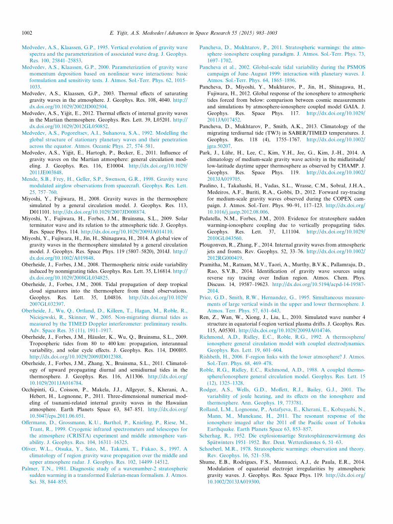
1002 E. Yigit, A.S. Medvedev / Advances in Space Research 55 (2015) 983–1003
Medvedev, A.S., Klaassen, G.P., 1995. Vertical evolution of gravity wavespectra and the parameterization of associated wave drag. J. Geophys.Res. 100, 25841–25853.
Medvedev, A.S., Klaassen, G.P., 2000. Parameterization of gravity wavemomentum deposition based on nonlinear wave interactions: basicformulation and sensitivity tests. J. Atmos. Sol.-Terr. Phys. 62, 1015–1033.
Medvedev, A.S., Klaassen, G.P., 2003. Thermal effects of saturatinggravity waves in the atmosphere. J. Geophys. Res. 108, 4040. http://dx.doi.org/10.1029/2002JD002504.
Medvedev, A.S., Yigit, E., 2012. Thermal effects of internal gravity wavesin the Martian thermosphere. Geophys. Res. Lett. 39, L05201. http://dx.doi.org/10.1029/2012GL050852.
Medvedev, A.S., Pogoreltsev, A.I., Suhanova, S.A., 1992. Modelling theglobal structure of stationary planetary waves and their penetrationacross the equator. Atmos. Oceanic Phys. 27, 574–581.
Medvedev, A.S., Yigit, E., Hartogh, P., Becker, E., 2011. Influence ofgravity waves on the Martian atmosphere: general circulation mod-eling. J. Geophys. Res. 116, E10004. http://dx.doi.org/10.1029/2011JE003848.
Mende, S.B., Frey, H., Geller, S.P., Swenson, G.R., 1998. Gravity wavemodulated airglow observations from spacecraft. Geophys. Res. Lett.25, 757–760.
Miyoshi, Y., Fujiwara, H., 2008. Gravity waves in the thermospheresimulated by a general circulation model. J. Geophys. Res. 113,D011101. http://dx.doi.org/10.1029/2007JD008874.
Miyoshi, Y., Fujiwara, H., Forbes, J.M., Bruinsma, S.L., 2009. Solarterminator wave and its relation to the atmospheric tide. J. Geophys.Res. Space Phys. 114. http://dx.doi.org/10.1029/2009JA014110.
Miyoshi, Y., Fujiwara, H., Jin, H., Shinagawa, H., 2014. A global view ofgravity waves in the thermosphere simulated by a general circulationmodel. J. Geophys. Res. Space Phys. 119 (5807–5820), 2014J. http://dx.doi.org/10.1002/A019848.
Oberheide, J., Forbes, J.M., 2008. Thermospheric nitric oxide variabilityinduced by nonmigrating tides. Geophys. Res. Lett. 35, L16814. http://dx.doi.org/10.1029/2008GL034825.
Oberheide, J., Forbes, J.M., 2008. Tidal propagation of deep tropicalcloud signatures into the thermosphere from timed observations.Geophys. Res. Lett. 35, L04816. http://dx.doi.org/10.1029/2007GL032397.
Oberheide, J., Wu, Q., Ortland, D., Killeen, T., Hagan, M., Roble, R.,Niciejewski, R., Skinner, W., 2005. Non-migrating diurnal tides asmeasured by the TIMED Doppler interferometer: preliminary results.Adv. Space Res. 35 (11), 1911–1917.
Oberheide, J., Forbes, J.M., Hausler, K., Wu, Q., Bruinsma, S.L., 2009.Tropospheric tides from 80 to 400 km: propagation, interannualvariability, and solar cycle effects. J. Geophys. Res. 114, D00I05.http://dx.doi.org/10.1029/2009JD012388.
Oberheide, J., Forbes, J.M., Zhang, X., Bruinsma, S.L., 2011. Climatol-ogy of upward propagating diurnal and semidiurnal tides in thethermosphere. J. Geophys. Res. 116, A11306. http://dx.doi.org/10.1029/2011JA016784.
Occhipinti, G., Coisson, P., Makela, J.J., Allgeyer, S., Kherani, A.,Hebert, H., Lognonne, P., 2011. Three-dimensional numerical mod-eling of tsunami-related internal gravity waves in the Hawaiianatmosphere. Earth Planets Space 63, 847–851. http://dx.doi.org/10.5047/eps.2011.06.051.
Offermann, D., Grossmann, K.U., Barthol, P., Knieling, P., Riese, M.,Trant, R., 1999. Cryogenic infrared spectrometers and telescopes forthe atmosphere (CRISTA) experiment and middle atmosphere vari-ability. J. Geophys. Res. 104, 16311–16325.
Oliver, W.L., Otsuka, Y., Sato, M., Takami, T., Fukao, S., 1997. Aclimatology of f region gravity wave propagation over the middle andupper atmosphere radar. J. Geophys. Res. 102, 14499–14512.
Palmer, T.N., 1981. Diagnostic study of a wavenumber-2 stratosphericsudden warming in a transformed Eulerian-mean formalism. J. Atmos.Sci. 38, 844–855.
Pancheva, D., Mukhtarov, P., 2011. Stratospheric warmings: the atmo-sphere–ionosphere coupling paradigm. J. Atmos. Sol.-Terr. Phys. 73,1697–1702.
Pancheva et al., 2002. Global-scale tidal variability during the PSMOScampaign of June–August 1999: interaction with planetary waves. J.Atmos. Sol.-Terr. Phys. 64, 1865–1896.
Pancheva, D., Miyoshi, Y., Mukhtarov, P., Jin, H., Shinagawa, H.,Fujiwara, H., 2012. Global response of the ionosphere to atmospherictides forced from below: comparison between cosmic measurementsand simulations by atmosphere-ionosphere coupled model GAIA. J.Geophys. Res. Space Phys. 117. http://dx.doi.org/10.1029/2011JA017452.
Pancheva, D., Mukhtarov, P., Smith, A.K., 2013. Climatology of themigrating terdiurnal tide (TW3) in SABER/TIMED temperatures. J.Geophys. Res. 118 (4), 1755–1767. http://dx.doi.org/10.1002/jgra.50207.
Park, J., Luhr, H., Lee, C., Kim, Y.H., Jee, G., Kim, J.-H., 2014. Aclimatology of medium-scale gravity wave activity in the midlatitude/low-latitude daytime upper thermosphere as observed by CHAMP. J.Geophys. Res. Space Phys. 119. http://dx.doi.org/10.1002/2013JA019705.
Paulino, I., Takahashi, H., Vadas, S.L., Wrasse, C.M., Sobral, J.H.A.,Medeiros, A.F., Buriti, R.A., Gobbi, D., 2012. Forward ray-tracingfor medium-scale gravity waves observed during the COPEX cam-paign. J. Atmos. Sol.-Terr. Phys. 90–91, 117–123. http://dx.doi.org/10.1016/j.jastp.2012.08.006.
Pedatella, N.M., Forbes, J.M., 2010. Evidence for stratosphere suddenwarming-ionosphere coupling due to vertically propagating tides.Geophys. Res. Lett. 37, L11104. http://dx.doi.org/10.1029/2010GL043560.
Plougonven, R., Zhang, F., 2014. Internal gravity waves from atmosphericjets and fronts. Rev. Geophys. 52, 33–76. http://dx.doi.org/10.1002/2012RG000419.
Pramitha, M., Ratnam, M.V., Taori, A., Murthy, B.V.K., Pallamraju, D.,Rao, S.V.B., 2014. Identification of gravity wave sources usingreverse ray tracing over Indian region. Atmos. Chem. Phys.Discuss. 14, 19587–19623. http://dx.doi.org/10.5194/acpd-14-19587-2014.
Price, G.D., Smith, R.W., Hernandez, G., 1995. Simultaneous measure-ments of large vertical winds in the upper and lower thermosphere. J.Atmos. Terr. Phys. 57, 631–643.
Ren, Z., Wan, W., Xiong, J., Liu, L., 2010. Simulated wave number 4structure in equatorial f-region vertical plasma drifts. J. Geophys. Res.115, A05301. http://dx.doi.org/10.1029/2009JA014746.
Richmond, A.D., Ridley, E.C., Roble, R.G., 1992. A thermosphere/ionosphere general circulation model with coupled electrodynamics.Geophys. Res. Lett. 19, 601–604.
Rishbeth, H., 2006. F-region links with the lower atmosphere? J. Atmos.Sol.-Terr. Phys. 68, 469–478.
Roble, R.G., Ridley, E.C., Richmond, A.D., 1988. A coupled thermo-sphere/ionosphere general circulation model. Geophys. Res. Lett. 15(12), 1325–1328.
Rodger, A.S., Wells, G.D., Moffett, R.J., Bailey, G.J., 2001. Thevariability of joule heating, and its effects on the ionosphere andthermosphere. Ann. Geophys. 19, 773781.
Rolland, L.M., Lognonne, P., Astafyeva, E., Kherani, E., Kobayashi, N.,Mann, M., Munekane, H., 2011. The resonant response of theionosphere imaged after the 2011 off the Pacific coast of TohokuEarthquake. Earth Planets Space 63, 853–857.
Scherhag, R., 1952. Die explosionsartige Stratospharenerwarmung desSpatwinters 1951–1952. Ber. Deut. Wetterdienstes 6, 51–63.
Schoeberl, M.R., 1978. Stratospheric warmings: observation and theory.Rev. Geophys. 16, 521–538.
Shume, E.B., Rodrigues, F.S., Mannucci, A.J., de Paula, E.R., 2014.Modulation of equatorial electrojet irregularities by atmosphericgravity waves. J. Geophys. Res. Space Phys. 119. http://dx.doi.org/10.1002/2013JA019300.
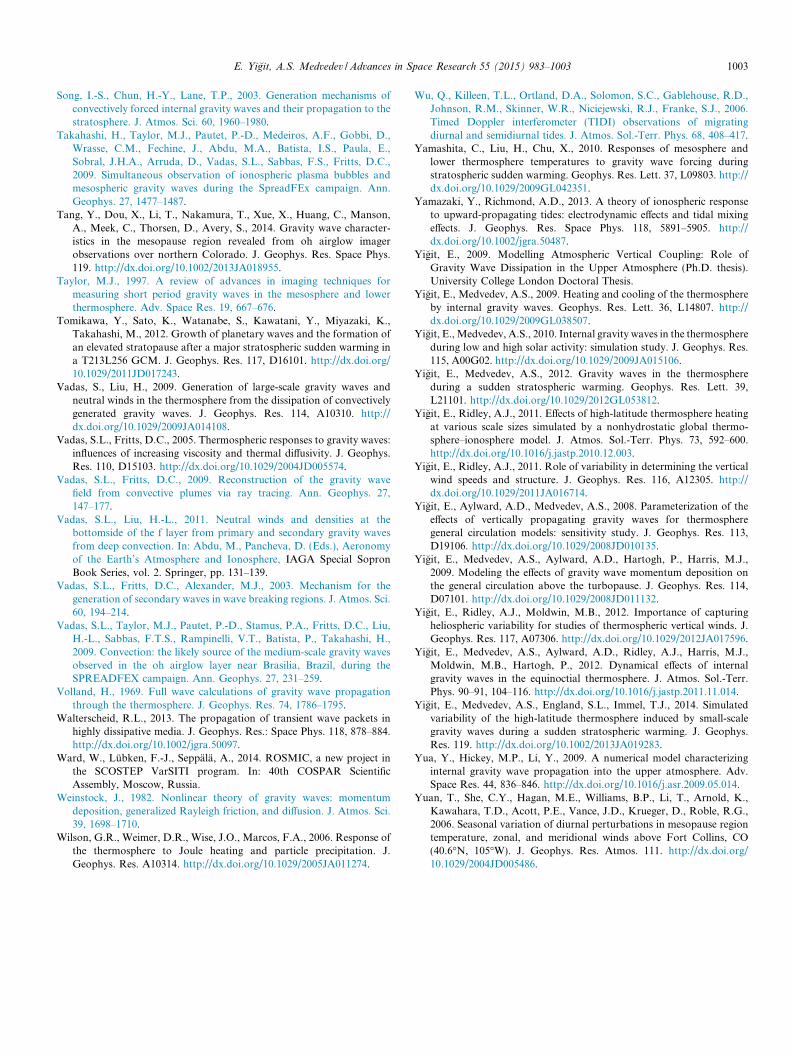
E. Yigit, A.S. Medvedev / Advances in Space Research 55 (2015) 983–1003 1003
Song, I.-S., Chun, H.-Y., Lane, T.P., 2003. Generation mechanisms ofconvectively forced internal gravity waves and their propagation to thestratosphere. J. Atmos. Sci. 60, 1960–1980.
Takahashi, H., Taylor, M.J., Pautet, P.-D., Medeiros, A.F., Gobbi, D.,Wrasse, C.M., Fechine, J., Abdu, M.A., Batista, I.S., Paula, E.,Sobral, J.H.A., Arruda, D., Vadas, S.L., Sabbas, F.S., Fritts, D.C.,2009. Simultaneous observation of ionospheric plasma bubbles andmesospheric gravity waves during the SpreadFEx campaign. Ann.Geophys. 27, 1477–1487.
Tang, Y., Dou, X., Li, T., Nakamura, T., Xue, X., Huang, C., Manson,A., Meek, C., Thorsen, D., Avery, S., 2014. Gravity wave character-istics in the mesopause region revealed from oh airglow imagerobservations over northern Colorado. J. Geophys. Res. Space Phys.119. http://dx.doi.org/10.1002/2013JA018955.
Taylor, M.J., 1997. A review of advances in imaging techniques formeasuring short period gravity waves in the mesosphere and lowerthermosphere. Adv. Space Res. 19, 667–676.
Tomikawa, Y., Sato, K., Watanabe, S., Kawatani, Y., Miyazaki, K.,Takahashi, M., 2012. Growth of planetary waves and the formation ofan elevated stratopause after a major stratospheric sudden warming ina T213L256 GCM. J. Geophys. Res. 117, D16101. http://dx.doi.org/10.1029/2011JD017243.
Vadas, S., Liu, H., 2009. Generation of large-scale gravity waves andneutral winds in the thermosphere from the dissipation of convectivelygenerated gravity waves. J. Geophys. Res. 114, A10310. http://dx.doi.org/10.1029/2009JA014108.
Vadas, S.L., Fritts, D.C., 2005. Thermospheric responses to gravity waves:influences of increasing viscosity and thermal diffusivity. J. Geophys.Res. 110, D15103. http://dx.doi.org/10.1029/2004JD005574.
Vadas, S.L., Fritts, D.C., 2009. Reconstruction of the gravity wavefield from convective plumes via ray tracing. Ann. Geophys. 27,147–177.
Vadas, S.L., Liu, H.-L., 2011. Neutral winds and densities at thebottomside of the f layer from primary and secondary gravity wavesfrom deep convection. In: Abdu, M., Pancheva, D. (Eds.), Aeronomyof the Earth’s Atmosphere and Ionosphere, IAGA Special SopronBook Series, vol. 2. Springer, pp. 131–139.
Vadas, S.L., Fritts, D.C., Alexander, M.J., 2003. Mechanism for thegeneration of secondary waves in wave breaking regions. J. Atmos. Sci.60, 194–214.
Vadas, S.L., Taylor, M.J., Pautet, P.-D., Stamus, P.A., Fritts, D.C., Liu,H.-L., Sabbas, F.T.S., Rampinelli, V.T., Batista, P., Takahashi, H.,2009. Convection: the likely source of the medium-scale gravity wavesobserved in the oh airglow layer near Brasilia, Brazil, during theSPREADFEX campaign. Ann. Geophys. 27, 231–259.
Volland, H., 1969. Full wave calculations of gravity wave propagationthrough the thermosphere. J. Geophys. Res. 74, 1786–1795.
Walterscheid, R.L., 2013. The propagation of transient wave packets inhighly dissipative media. J. Geophys. Res.: Space Phys. 118, 878–884.http://dx.doi.org/10.1002/jgra.50097.
Ward, W., Lubken, F.-J., Seppala, A., 2014. ROSMIC, a new project inthe SCOSTEP VarSITI program. In: 40th COSPAR ScientificAssembly, Moscow, Russia.
Weinstock, J., 1982. Nonlinear theory of gravity waves: momentumdeposition, generalized Rayleigh friction, and diffusion. J. Atmos. Sci.39, 1698–1710.
Wilson, G.R., Weimer, D.R., Wise, J.O., Marcos, F.A., 2006. Response ofthe thermosphere to Joule heating and particle precipitation. J.Geophys. Res. A10314. http://dx.doi.org/10.1029/2005JA011274.
Wu, Q., Killeen, T.L., Ortland, D.A., Solomon, S.C., Gablehouse, R.D.,Johnson, R.M., Skinner, W.R., Niciejewski, R.J., Franke, S.J., 2006.Timed Doppler interferometer (TIDI) observations of migratingdiurnal and semidiurnal tides. J. Atmos. Sol.-Terr. Phys. 68, 408–417.
Yamashita, C., Liu, H., Chu, X., 2010. Responses of mesosphere andlower thermosphere temperatures to gravity wave forcing duringstratospheric sudden warming. Geophys. Res. Lett. 37, L09803. http://dx.doi.org/10.1029/2009GL042351.
Yamazaki, Y., Richmond, A.D., 2013. A theory of ionospheric responseto upward-propagating tides: electrodynamic effects and tidal mixingeffects. J. Geophys. Res. Space Phys. 118, 5891–5905. http://dx.doi.org/10.1002/jgra.50487.
Yigit, E., 2009. Modelling Atmospheric Vertical Coupling: Role ofGravity Wave Dissipation in the Upper Atmosphere (Ph.D. thesis).University College London Doctoral Thesis.
Yigit, E., Medvedev, A.S., 2009. Heating and cooling of the thermosphereby internal gravity waves. Geophys. Res. Lett. 36, L14807. http://dx.doi.org/10.1029/2009GL038507.
Yigit, E., Medvedev, A.S., 2010. Internal gravity waves in the thermosphereduring low and high solar activity: simulation study. J. Geophys. Res.115, A00G02. http://dx.doi.org/10.1029/2009JA015106.
Yigit, E., Medvedev, A.S., 2012. Gravity waves in the thermosphereduring a sudden stratospheric warming. Geophys. Res. Lett. 39,L21101. http://dx.doi.org/10.1029/2012GL053812.
Yigit, E., Ridley, A.J., 2011. Effects of high-latitude thermosphere heatingat various scale sizes simulated by a nonhydrostatic global thermo-sphere–ionosphere model. J. Atmos. Sol.-Terr. Phys. 73, 592–600.http://dx.doi.org/10.1016/j.jastp.2010.12.003.
Yigit, E., Ridley, A.J., 2011. Role of variability in determining the verticalwind speeds and structure. J. Geophys. Res. 116, A12305. http://dx.doi.org/10.1029/2011JA016714.
Yigit, E., Aylward, A.D., Medvedev, A.S., 2008. Parameterization of theeffects of vertically propagating gravity waves for thermospheregeneral circulation models: sensitivity study. J. Geophys. Res. 113,D19106. http://dx.doi.org/10.1029/2008JD010135.
Yigit, E., Medvedev, A.S., Aylward, A.D., Hartogh, P., Harris, M.J.,2009. Modeling the effects of gravity wave momentum deposition onthe general circulation above the turbopause. J. Geophys. Res. 114,D07101. http://dx.doi.org/10.1029/2008JD011132.
Yigit, E., Ridley, A.J., Moldwin, M.B., 2012. Importance of capturingheliospheric variability for studies of thermospheric vertical winds. J.Geophys. Res. 117, A07306. http://dx.doi.org/10.1029/2012JA017596.
Yigit, E., Medvedev, A.S., Aylward, A.D., Ridley, A.J., Harris, M.J.,Moldwin, M.B., Hartogh, P., 2012. Dynamical effects of internalgravity waves in the equinoctial thermosphere. J. Atmos. Sol.-Terr.Phys. 90–91, 104–116. http://dx.doi.org/10.1016/j.jastp.2011.11.014.
Yigit, E., Medvedev, A.S., England, S.L., Immel, T.J., 2014. Simulatedvariability of the high-latitude thermosphere induced by small-scalegravity waves during a sudden stratospheric warming. J. Geophys.Res. 119. http://dx.doi.org/10.1002/2013JA019283.
Yua, Y., Hickey, M.P., Li, Y., 2009. A numerical model characterizinginternal gravity wave propagation into the upper atmosphere. Adv.Space Res. 44, 836–846. http://dx.doi.org/10.1016/j.asr.2009.05.014.
Yuan, T., She, C.Y., Hagan, M.E., Williams, B.P., Li, T., Arnold, K.,Kawahara, T.D., Acott, P.E., Vance, J.D., Krueger, D., Roble, R.G.,2006. Seasonal variation of diurnal perturbations in mesopause regiontemperature, zonal, and meridional winds above Fort Collins, CO(40.6�N, 105�W). J. Geophys. Res. Atmos. 111. http://dx.doi.org/10.1029/2004JD005486.
Related Documents