Interest Rates Under Falling Stars - Federal Reserve … appear to have slowly altered global saving and investment and, in turn, pushed down the steady-state ... Interest Rates Under

FEDERAL RESERVE BANK OF SAN FRANCISCO

WORKING PAPER SERIES

Interest Rates Under Falling Stars

Michael D. Bauer and Glenn D. Rudebusch Federal Reserve Bank of San Francisco

November 2017

Working Paper 2017-16 http://www.frbsf.org/economic-research/publications/working-papers/2017/16/

Suggested citation:

Bauer, Michael D., Glenn D. Rudebusch. 2017. “Interest Rates Under Falling Stars” Federal Reserve Bank of San Francisco Working Paper 2017-16. https://doi.org/10.24148/wp2017-16 The views in this paper are solely the responsibility of the authors and should not be interpreted as reflecting the views of the Federal Reserve Bank of San Francisco or the Board of Governors of the Federal Reserve System.

Interest Rates Under Falling Stars

Michael D. Bauer and Glenn D. Rudebusch∗

Federal Reserve Bank of San Francisco

November 17, 2017

Abstract

While theory predicts that the equilibrium real interest rate, r∗t , and the perceived trend

in inflation, π∗t , are fundamental determinants of the yield curve, macro-finance models

generally treat them as constant. We show that accounting for time-varying macro

trends is critical for understanding the empirical dynamics of U.S. Treasury yields and

risk pricing. It fundamentally changes estimated risk premiums in long-term bond yields,

leads to large gains in predictions of excess bond returns and long-range out-of-sample

forecasts of interest rates, and captures a substantial share of interest rate variability at

low frequencies.

Keywords: yield curve, macro-finance, inflation trend, equilibrium real interest rate,

shifting endpoints, bond risk premiums

JEL Classifications: E43, E44, E47

∗Michael D. Bauer ([email protected]), Glenn D. Rudebusch ([email protected]): Eco-nomic Research Department, Federal Reserve Bank of San Francisco, 101 Market Street, San Francisco, CA94105. We thank Anna Cieslak, Todd Clark, John Cochrane, Robert Hodrick, Lars Svensson, Jonathan Wrightand seminar participants at various institutions for helpful comments; Elmar Mertens, Mike Kiley and ThomasLubik for their r∗t estimates; and Simon Riddell and Logan Tribull for excellent research assistance. The viewsin this paper are solely the responsibility of the authors and do not necessarily reflect those of others in theFederal Reserve System.

1 Introduction

Research in financial economics has made numerous attempts to connect macroeconomic vari-

ables to the term structure of interest rates using a variety of approaches ranging from reduced-

form no-arbitrage models to fully-fledged dynamic macro models.1 Despite both theoretical

and empirical progress, there is no clear consensus about how macroeconomic information

should be incorporated into yield-curve analysis. Notably, two widely cited estimates of the

term premium in long-term yields by Kim and Wright (2005) and Adrian et al. (2013) are based

on models that include no macroeconomic data. One important link between the macroecon-

omy and the yield curve that has been largely overlooked is the connection between their

long-run trends.2 Specifically, macroeconomic data and models can provide estimates of the

trend in inflation (π∗t ) and the equilibrium real interest rate (r∗t ), and finance theory—from

Irving Fisher through modern no-arbitrage models—tells us that such macroeconomic trends

must be reflected in interest rates. Of course, as an empirical issue, what matters is whether

there is significant variation over time in these long-run trends. Almost all term structure

analyses assume that these variables are constant. Instead, in this paper, we document that

accounting for the macro-finance link between a time-varying π∗t and r∗t and the long-run trend

in interest rates is essential for modeling the term structure, estimating bond risk premiums,

and forecasting the yield curve.

An illustration of the potential importance of macro trends is provided in Figure 1. The

secular decline in the 10-year Treasury yield since the early 1980s reflects a gradual down-

trend in the general level of U.S. interest rates. The underlying drivers of this decline and their

dynamics remain contentious. In finance, specifically in no-arbitrage term structure models,

interest rates are generally modeled as stationary, mean-reverting processes, because over very

long historical periods they have always remained range-bound. As a result, low-frequency

variation in interest rates is hard to explain in such models, and it is mostly attributed to

the residual term premium component, the difference between a long-term interest rate and

the model-implied expectations of average future short-term rates. A prominent example

is Wright (2011), who concluded that between 1990 and 2010 interest rates fell globally be-

cause of declining term premiums that in turn reflected a decrease in inflation uncertainty.

However, our estimates of the trends underlying interest rates displayed in Figure 1 suggest a

very different explanation. First, our measure of U.S. trend inflation, based on long-horizon

1See Ang and Piazzesi (2003), Diebold et al. (2006), Rudebusch and Wu (2008), Bikbov and Chernov(2010), Rudebusch and Swanson (2012), Bansal and Shaliastovich (2013), and Joslin et al. (2014), amongmany others. For a detailed survey, see Gurkaynak and Wright (2012).

2Throughout this paper, we use the Beveridge-Nelson concept of a trend, that is, the expectation for aneconomic series in the (infinitely) distant future.

1

inflation survey forecasts, declined by almost six percentage points from the early 1980s to the

late 1990s. Hence, expectations about the level of inflation must have played an important

role in pushing down nominal yields. Second, over the past two decades as inflation expec-

tations have stabilized, our estimate of the equilibrium real interest rate (which is described

in detail below) has exhibited a pronounced decline.3 This drop implies that the component

capturing expectations of future real interest rates helped push interest rates lower as well.

The expectations component of nominal yields necessarily contains the sum of both macro

trends, i∗t = π∗t + r∗t , i.e., the equilibrium nominal short rate. As evident in Figure 1, our

estimate of i∗t exhibited similar low-frequency movements as the ten-year Treasury yield. This

strongly suggests that the earlier downward trend in π∗t and the more recent fall in r∗t—that is,

an environment of falling stars—is the main reason for the secular decline in nominal interest

rates. Indeed, given the fall in i∗t there is little room for secular trends in the term premium

to account for this decline.

In this paper we quantify the importance of i∗t , π∗t , and r?t for the evolution of the yield

curve using standard empirical proxies for these macro trends and five different empirical

approaches. First, we investigate the link between yields and macro trends using standard

time series methods. This analysis reveals that time variation in both π∗t and r∗t is responsible

for the extremely high persistence of interest rates. The difference between long-term interest

rates and i∗t exhibits quick mean reversion, and tests for unit roots and cointegration clearly

indicate that π∗t and r∗t account for the trend component in nominal yields. Accounting only

for the inflation trend on its own, as in Kozicki and Tinsley (2001) and Cieslak and Povala

(2015), leaves a highly persistent component of interest rates unexplained. Accordingly, we

show that it is crucial to include r∗t as well—given the quantitatively important changes in

the equilibrium real rate—in order to fully capture the trend component in interest rates.

After accounting for shifts in r∗t , we uncover strong evidence for a long-run Fisher effect in

which long-term interest rates and inflation share a common trend. Previous studies have

found mixed results on the Fisher effects, because they focus only on a bivariate relationship

between yields and inflation (Mishkin, 1992; Wallace and Warner, 1993; Evans and Lewis,

1995). We also document, using a simple error-correction model, that the long-term yields

quickly revert back to their underlying macro trend i∗t .

Second, we estimate predictive regressions for excess bond returns in order to understand

3 Various underlying fundamental economic forces, such as lower productivity growth and an aging popu-lation, appear to have slowly altered global saving and investment and, in turn, pushed down the steady-statereal interest rate. Discussions of the decline in r∗ include Summers (2014), Rachel and Smith (2015), Hamiltonet al. (2016), Holston et al. (2017), Del Negro et al. (2017), and many others. In the macroeconomics literature,r∗t is often labeled the neutral or natural rate of interest although, as noted below, there are various definitionswith subtle differences.

2

the role of macro trends for bond risk premiums. Accounting for changes in the underlying

macro trends fundamentally changes return predictions. Relative to the standard predictive

regressions for excess bond returns using current yields, both π∗t and r∗t have strong incremental

predictive power. Consistent with the intuition from Figure 1, the addition of the equilibrium

real rate is crucial later in our sample, when the inflation trend shows less variation. This

explains why the fit of the regressions of Cieslak and Povala (2015), who predict bond returns

using a moving average of past inflation, has diminished over time. Including i∗t as a predictor

fully captures the relevant information in macro trends, and the predictive gains are econom-

ically large: a decline of one percentage point in the trend component predicts an increase

in the future annual excess returns by about 7.5 percentage points, as interest rates quickly

mean-revert to the lower trend and long-term bond holders benefit, just as they have during

the recent period since the Financial Crisis. A parsimonious and effective way to uncover the

predictive power in yields is by detrending them, i.e., by focusing on the difference between

yields and their underlying macro trend. Our findings extend recent research on predictions

of excess bond returns (Cieslak and Povala, 2015; Brooks and Moskowitz, 2017; Garg and

Mazzoleni, 2017; Jorgensen, 2017) which documented some gains from including slow-moving

averages of past inflation and real GDP or consumption growth as predictors. We show that

large gains result from accounting for the underlying macro trends π∗t and r∗t , and that the

underlying mechanism is mean-reversion of yields to i∗t . In addition, we provide an explanation

why expected returns are not spanned by the yield curve: Because changes in the level of the

yield curve can occur due to either movements in i∗t or level shifts in detrended yields—with

very different implications for expectations of future returns—macro trends and yields contain

important separate pieces of predictive information.

Third, we turn to out-of-sample forecasting of interest rates. In such forecasting exercises,

researchers have found it surprisingly difficult to consistently beat the simple random walk

forecast, which predicts future yields with current yields. But we find that simple univariate

predictions in which long-term interest rates mean-revert to the shifting endpoint i∗t leads to

substantial forecast gains at medium and long forecast horizons relative to the usual martingale

benchmark. These improvements in forecast accuracy are both economically and statistically

significant, and they are consistent with the notion of equilibrium correction of yields to

their underlying macro trends. Our forecasts also consistently beat long-range projections

from the Blue Chip survey of professional forecasters. In related previous work, Dijk et al.

(2014) documented some forecast improvements relative to a random walk by including shifting

endpoints that are linear projections based on their proxy of π∗t . We demonstrate that no linear

projections are needed and that the right endpoint to use is i∗t , which importantly includes r∗t .

3

Fourth, we investigate the role of macro trends for the term premium and revisit the secu-

lar decline in long-term interest rates. We obtain a novel estimate of the term premium using

a simple factor model of the yield curve in which three factors of detrended yields follow a

first-order vector autoregression (VAR), so that yields revert to a shifting endpoint that is

determined by i∗t . The resulting empirical decomposition of long-term rates into expectations

and term premium components starkly contrasts with that from a conventional yield-curve

model in which yield factors follow a stationary VAR(1). The conventional decomposition

implies an implausibly stable expectations component and attributes most of the secular de-

cline in interest rates to the residual term premium, as discussed in critiques by Kim and

Orphanides (2012) and Bauer et al. (2014). Our decomposition instead attributes the ma-

jority of the secular decline to the decrease in i∗t . Consequently, the term premium, instead

of exhibiting a dubious secular downtrend, behaves in a predominantly cyclical fashion like

other risk premiums in asset prices (Fama and French, 1989). Linking macro trends to the

yield curve solves the knife-edge problem of Cochrane (2007), who noted that assuming either

stationary or martingale interest rates leads to drastically different implications for the term

premium. Assuming a common macro trend, as prescribed by theory, leads to both more ac-

curate forecasts and to more plausible decompositions of long-term rates than either of those

previous methods.4

As a final avenue of examination, we compare the variance of changes in macro trends to

the variance of interest rate changes at different frequencies. Duffee (2016) proposes using the

ratio of the variance of inflation news to the variance of yield innovations as a useful metric

to assess the importance of inflation in the determination of interest rates. He documents

that for one-quarter innovations, this ratio is small for U.S. Treasury yields. We generalize

his measure to consider variance ratios for longer h-period innovations, which allows us to

compare the size of unexpected changes, over, say, a span of five years, in inflation and in

nominal bond yields. For one-quarter changes, we replicate the small inflation variance ratio

reported by Duffee. But the inflation variance ratio increases substantially with the horizon, as

one would expect if inflation has an important trend component. We also generalize Duffee’s

measure to incorporate fluctuations in r∗t and i∗t . Although confidence intervals are unavoidably

wide, our estimates suggest that during the postwar U.S. sample, a large share of the interest

rate variability faced by investors over longer holding periods was due to changes in the

macroeconomic trend components of nominal yields.

4Our analysis of the term premium is related to recent work by Crump et al. (2017), who also allow for slow-moving macroeconomic trends but, in contrast, find that a substantial downward trend in the term premiumis the main driver of lower bond yields. The key difference with our approach is their exclusive reliance onsurvey measures for estimation of i∗t , which as we discuss below is problematic.

4

While it has long been recognized that nominal interest rates contain a slow-moving trend

component (Nelson and Plosser, 1982; Rose, 1988), our paper is the first empirical work that

fully explains this trend by linking it to the macroeconomy. We identify the underlying

macroeconomic drivers of i∗t , and document that these fluctuations are quantitatively impor-

tant. In previous work, filtering i∗t from past yield curve data alone has generally proved to

be an unsuccessful strategy (Fama, 2006; Dijk et al., 2014; Cieslak and Povala, 2015). Some

studies have found a link between the inflation trend and nominal yields (Kozicki and Tinsley,

2001; Dijk et al., 2014; Cieslak and Povala, 2015), but this leaves unexplained the continuing

downtrend trend in yields over the last 20 years. We comprehensively document the empirical

importance of macro trends for the dynamics of the yield curve, demonstrating the effects of

both relevant macro trends, π∗t and r∗t . Time variation in r∗t has so far been largely ignored

in finance, which is a substantial oversight given the extensive evidence in the recent macro

literature on the equilibrium real interest rate and its structural drivers.

Our work has important implications not only for forecasting of interest rates and bond

returns, but also for macro-finance modeling of the yield curve. Existing yield-curve models

generally do not account for the crucial link between macro and yield trends. Macro-finance

no-arbitrage models of the yield curve (see the references in Footnote 1) generally impose

stationary dynamics and do not allow for time-varying macro trends, ruling out the structural,

long-run changes which we demonstrate to be empirically important.5 In light of our findings,

it is paramount for yield-curve models to explicitly allow for macroeconomic trends to affect

long-run expectations of interest rates.

2 Some theory: macro trends and yields

Absence of arbitrage implies that expectations of future macroeconomic variables are linked

to long-term interest rates (Ang and Piazzesi, 2003; Rudebusch and Wu, 2008). Specifically,

the yield on a long-term bond is driven by expectations of future inflation and expectations

of future real rates, plus a risk premium that depends on the specific asset-pricing model.

Here we discuss the implications for yield-curve dynamics if inflation or the real rate contain

time-varying trend components.

According to the prevailing consensus in empirical macroeconomics—prominently exempli-

fied by Stock and Watson (2007) and recently surveyed in Faust and Wright (2013)—inflation

5Some general-equilibrium macro models allow for changes in the inflation trend that are linked to the yieldcurve but assume a constant equilibrium real rate (Hordahl et al., 2006; Rudebusch and Wu, 2008). Certainno-arbitrage models developed by Hand Dewachter and coauthors allow for changes in r∗ but make strongassumptions such as deterministically linking r∗t to π∗t (Dewachter and Lyrio, 2006) or imposing that r∗t equalstrend output growth (Dewachter and Iania, 2011).

5

is best modeled as an I(1) process if one aims to produce competitive forecasts or accurately

capture the evolution of expectations. Hence, a Beveridge-Nelson trend can be defined as

π∗t = limh→∞

Etπt+h,

assuming that inflation does not have a deterministic trend. From a macroeconomic perspec-

tive, this time-varying inflation endpoint can be viewed as the perceived inflation target of the

central bank. Inflation can thus be modeled as the sum of a (random walk) trend component

and a (stationary) cycle component as in this simple formulation:

πt+1 = π∗t + ct + et+1, π∗t = π∗t−1 + ξt, ct = φcct−1 + ut, (1)

where the innovations ξt and ut and the noise component et are all iid. Expectations at t

about future inflation from t+ h to t+ h+ 1 are given as Etπt+h+1 = π∗t + φhc ct. We will use

this specification, which is similar to the one in Duffee (2016), to help illustrate the role of

trend and cycle in a bond pricing equation in a no-arbitrage term structure framework.6

A similar specification is also relevant for the real interest rate. Structural economic

changes, such as changes in the trend rates of productivity and population growth, will affect

the equilibrium real rate (see Footnote 3). These provide compelling reasons to allow for the

presence of a time-varying trend component in real interest rates, so we also assume that the

one-period real rate, rt, is I(1). We define the equilibrium real rate as the Beveridge-Nelson

trend,

r∗t = limh→∞

Etrt+h,

which can be understood as the real rate that prevails in the economy after all shocks have

died out. We discuss in Section 3 how this definition relates to other empirical and theoretical

concepts of what has come to be called “r-star” in the literature. Again a simple parametric

specification can best illustrate the implications of the presence of a trend in the real rate:

rt = r∗t + gt, r∗t = r∗t−1 + ηt, gt = φggt−1 + vt, (2)

where the cyclical real-rate gap, gt, captures among other factors variation in the real short

rate due to monetary policy (Neiss and Nelson, 2003).

We should stress that the assumption of unit roots in inflation and the real rate is merely

6Note that in this specification, the Beveridge-Nelson cycle includes both an AR(1) process (ct) and mea-surement error (et+1). Equation (1) assumes that the shocks ξt and ut affect only expectations of futureinflation but not current inflation, which slightly simplifies the bond pricing formulas but has no fundamentalsignificance.

6

a convenient way to model these very persistent processes. It simplifies the exposition of our

model and the arguments regarding trend components, but it is not crucial. Taken literally,

a unit root specification is implausible because the forecast error variances of inflation and

real rates do not in fact increase linearly with the forecast horizon as predicted by a unit

root. Instead, both variables have always remained within certain bounds. However, in

finite samples, a stationary process can always be approximated arbitrarily well by a unit

root process, and it is well-known that doing so can often be beneficial for forecasting (e.g.,

Campbell and Perron, 1991). Therefore the unit root assumption is false if taken literally

but nevertheless very useful (like all models, according to the famous dictum). The trend

components π∗t and r∗t can be viewed as highly persistent components of πt and rt that capture

expectations at the long horizons relevant for investors, even if infinite-horizon expectations

are constant. In practice, these relevant time horizons are often in the 5- to 10-year range when

cyclical shocks have largely dissipated, as noted by Laubach and Williams (2003) and Summers

(2015).

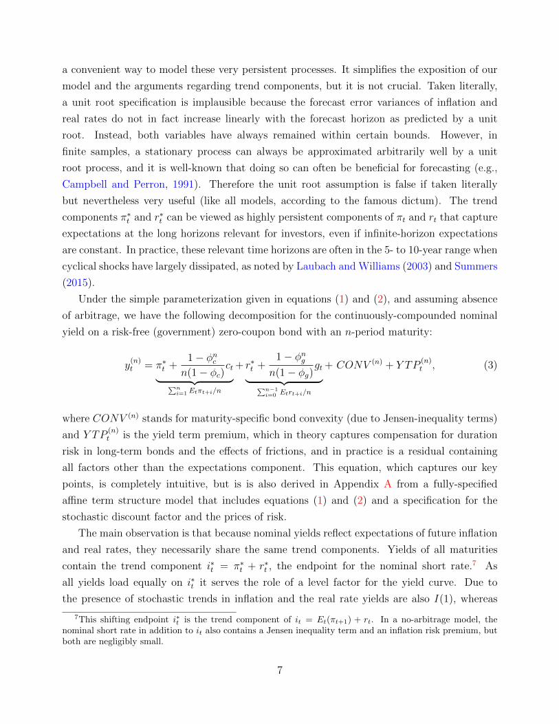
Under the simple parameterization given in equations (1) and (2), and assuming absence

of arbitrage, we have the following decomposition for the continuously-compounded nominal

yield on a risk-free (government) zero-coupon bond with an n-period maturity:

y(n)t = π∗t +

1 − φncn(1 − φc)

ct︸ ︷︷ ︸∑ni=1 Etπt+i/n

+ r∗t +1 − φng

n(1 − φg)gt︸ ︷︷ ︸∑n−1

i=0 Etrt+i/n

+ CONV (n) + Y TP(n)t , (3)

where CONV (n) stands for maturity-specific bond convexity (due to Jensen-inequality terms)

and Y TP(n)t is the yield term premium, which in theory captures compensation for duration

risk in long-term bonds and the effects of frictions, and in practice is a residual containing

all factors other than the expectations component. This equation, which captures our key

points, is completely intuitive, but is is also derived in Appendix A from a fully-specified

affine term structure model that includes equations (1) and (2) and a specification for the

stochastic discount factor and the prices of risk.

The main observation is that because nominal yields reflect expectations of future inflation

and real rates, they necessarily share the same trend components. Yields of all maturities

contain the trend component i∗t = π∗t + r∗t , the endpoint for the nominal short rate.7 As

all yields load equally on i∗t it serves the role of a level factor for the yield curve. Due to

the presence of stochastic trends in inflation and the real rate yields are also I(1), whereas

7This shifting endpoint i∗t is the trend component of it = Et(πt+1) + rt. In a no-arbitrage model, thenominal short rate in addition to it also contains a Jensen inequality term and an inflation risk premium, butboth are negligibly small.

7

detrended yields, y(n)t − i∗t , are I(0). These detrended yields, or “interest rate cycles” in the

parlance of Cieslak and Povala (2015), will play an important role in the empirical analysis

below.

The cyclical components ct and gt are slope factors as they affect short-term yields more

strongly than long-term yields. That the loadings of yields on these factors decline to zero

with increasing maturity is particularly easy to see in equation (3) because gt and ct follow

AR(1) processes, but it is true more generally for stationary yield-curve factors. Since the

cycles play a smaller role for long-term yields, we will focus most of our empirical analysis on

long-term yields and forward rates, to most clearly see the link between macro trends and the

yield curve.

Equation (3) can be viewed as an extended Fisher equation for long-term interest rates.

It suggests that loadings on inflation expectations are unity for all maturities, and hence that

there is long-run Fisher effect, i.e., that inflation and yields share the same long-run trend.

But we have so far focused only on the expectations component of long-term yields, and said

little about risk-adjustment and the term premium. Yields are driven by expectations of

future short rates under an adjusted, risk-neutral probability measure, and the term premium

in (3) captures this adjustment. If pi∗t directly affected the prices of risk, then Y TP(n)t would

systematically vary with changes in π∗t . In this case, the loadings of long-term yields on π∗t

would not necessarily be unity.8 The same reasoning of course holds for r∗t . In other words,

there is a clear theoretical prediction about the connection between macro trends and yields

through the expectations component, but this could be altered or even partially undone by the

term premium. However, we will present evidence that macro trends indeed appear to affect

long-term yields one-for-one, suggesting that the any possible links between macro trends and

the term premium are not strong enough to appreciably alter the role for macro trends in the

yield curve.

While standard theory predicts that the persistent components in inflation and the real

interest rate will be reflected in long-term interest rates, the key open question that we con-

sider is whether this link between macro trends and the yield curve matters empirically. How

important was variation in i∗t for the Treasury yield curve? We will demonstrate that account-

ing for changes in i∗t substantially alters our interpretation of yield curve movements and our

understanding of bond risk premiums.

8Technically speaking, we assumed that inflation has a unit root under the real-world probability measure,but this does not necessarily imply that it also has a unit root under the risk-neutral measure. In the model inAppendix A, we additionally assume that the term premium is not systematically affected by macro trends, sothat inflation and the real rate consequently also have a unit root under the risk-neutral measure, and yieldshave unit loadings on macro trends.

8

3 Data and trend estimates

We now describe the data and the estimates of the macroeconomic trends that we will use

in testing the model’s predictions. Our data set is quarterly and extends from 1971:Q4 to

2017:Q2. The interest rate data are end-of-quarter zero-coupon Treasury yields from Gurkaynak

et al. (2007) with maturities from one to 15 years. We augment these data with three- and

six-month Treasury bill rates from the Federal Reserve’s H.15 data. In our empirical analysis,

we mainly focus on long-term (five-year and ten-year) yields as well as long-term (five-to-ten-

year) forward rates to exhibit the importance of r∗t , π∗t , and r∗t , and these are the relevant

horizons for our trend measures as well.

For our empirical investigation, we take existing estimates of the macro trends from the

literature. Our goal is to assess whether such off-the-shelf measures can provide evidence

linking the inflation and real rate trends to the yield curve and risk pricing. An alternative

strategy would be to estimate time-varying r∗t and π∗t within a no-arbitrage term structure

model. We view our approach, which conditions on existing estimates, as an important first

step with two important advantages. First, our approach is arguably conservative, because our

macro trend estimates have not been fine-tuned to incorporate the information in long-term

yields via no-arbitrage restrictions. We avoid using trend estimates from the literature that

are derived from long-term yields, such as the estimates of π∗t by Christensen et al. (2010)

or estimates of r∗t by Johannsen and Mertens (2016), Christensen and Rudebusch (2017),

or Del Negro et al. (2017). It would be somewhat tautological to demonstrate a link between

long-term bond yields and a trend that was estimated from those yields. Because all of our

empirical trend proxies are based only on information in macroeconomic variables, short-term

interest rates, and surveys, we avoid any such circularity. Second, the estimation of macro

trends, in particular of r∗t , requires many difficult modeling decisions and, in the case of

Bayesian estimation, the choice of priors, all of which have important effects on the properties

of the estimated trend series.9 We prefer to instead use widely-used existing measures of the

macro trends and focus on how these trends relate to the yield curve.

Empirical proxies for trend inflation, π∗t , have been often constructed from surveys, sta-

tistical models, or a combination of the two—see, for example, Stock and Watson (2016) and

the references therein. We employ a well-known survey-based measure, namely, the Federal

Reserve’s series on the perceived inflation target rate, denoted PTR. It measures long-run

expectations of inflation in the price index of personal consumption expenditure (PCE), and

is widely used in empirical work—see, for example, Clark and McCracken (2013). PTR is

9For example, Laubach and Williams (2003) highlight the estimation and specification uncertainty under-lying their estimate of r∗t .

9

based exclusively on survey expectations since 1979 (i.e., for most of our sample).10 Figure 1

shows that from the beginning of our sample to the late 1990s, this estimate mostly mirrored

the increase and decrease in the ten-year yield. Since then, however, it has been essentially

flat at two percent, which is the level of the longer-run inflation goal of the Federal Reserve

that was first announced in 2012. Other survey expectations of inflation over the longer run,

such as the long-range forecasts in the Blue Chip survey, exhibit a similar pattern.11

The recent literature on modeling and estimation of the natural, neutral, or equilibrium real

interest rate—commonly referred to as r∗—has grown rapidly. Importantly, there are various

closely related definitions and concepts of r∗. Since we require estimates that are consistent

with our definition of the equilibrium real rate, it is useful to briefly review these concepts

here. In dynamic stochastic general equilibrium models (e.g. Curdia et al., 2015), the natural

or efficient real rate is the real rate that would prevail in the absence of nominal frictions.

This is generally a stationary variable and corresponds to a short-run concept. By contrast,

our definition of r∗ as the (Beveridge-Nelson) long-run trend component of the real interest

rate is a long-run concept. It coincides with the definition used in Lubik and Matthes (2015)

who estimate r∗t as the time-varying mean of the real rate in a time-varying parameter VAR

model.12 Another concept of the natural rate, used by Laubach and Williams (2003) and Kiley

(2015), among others, is the real rate at which monetary policy is neither expansionary nor

contractionary. In these models the unobserved natural rate is inferred from macroeconomic

data using a simple structural specification and the Kalman filter—Laubach and Williams

work with a standard IS curve whereas Kiley augments the IS curve with financial conditions.

While their r∗t is a medium-run concept because this neutral policy stance could in principle

change over time, it is specified in these models as a random walk, so that the medium-run

and long-run concepts coincide and this r∗t is consistent with our definition. We will therefore

use the three model-based estimates of Laubach and Williams (2003), Kiley (2015) and Lubik

and Matthes (2015) in our analysis.13

Figure 2 plots these three macro estimates of r∗t , and it shows that since the early 1980s, all

10Since 1979, PTR corresponds to long-run inflation expectations from the Survey of Professional Fore-casters. Before 1979, PTR is based on estimates from the learning model for expected inflation of Koz-icki and Tinsley (2001). For details on the construction of PTR, see Brayton and Tinsley (1996). PTRcan be downloaded with the updates of the Federal Reserve’s FRB/US large-scale macroeconomic model athttps://www.federalreserve.gov/econresdata/frbus/us-models-package.htm.

11The inflation trend that Cieslak and Povala (2015) use is a simple weighted moving average of past coreinflation, which, as they note, co-moves closely with PTR.

12Other estimates of this long-run r∗t include Johannsen and Mertens (2016) and Del Negro et al. (2017).13Survey-based estimates of r∗t are problematic for at least two reasons. First, the available time span for

interest rate forecasts is limited (the earliest is a biannual Blue Chip Financial Forecasts series that starts in1986). Second, this would amount to estimating i∗t as the long-run survey expectations of yields, which leadsto inaccurate forecasts as documented in previous studies (e.g., Dijk et al., 2014) and in Section 6.

10

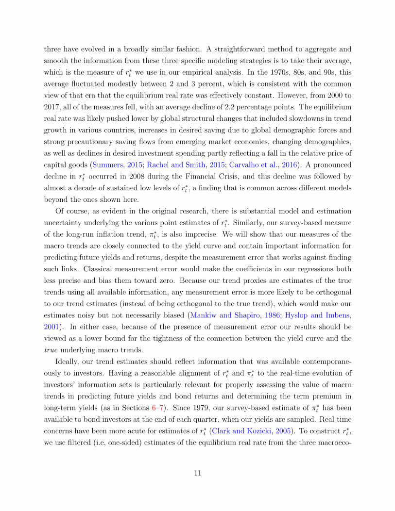
three have evolved in a broadly similar fashion. A straightforward method to aggregate and

smooth the information from these three specific modeling strategies is to take their average,

which is the measure of r∗t we use in our empirical analysis. In the 1970s, 80s, and 90s, this

average fluctuated modestly between 2 and 3 percent, which is consistent with the common

view of that era that the equilibrium real rate was effectively constant. However, from 2000 to

2017, all of the measures fell, with an average decline of 2.2 percentage points. The equilibrium

real rate was likely pushed lower by global structural changes that included slowdowns in trend

growth in various countries, increases in desired saving due to global demographic forces and

strong precautionary saving flows from emerging market economies, changing demographics,

as well as declines in desired investment spending partly reflecting a fall in the relative price of

capital goods (Summers, 2015; Rachel and Smith, 2015; Carvalho et al., 2016). A pronounced

decline in r∗t occurred in 2008 during the Financial Crisis, and this decline was followed by

almost a decade of sustained low levels of r∗t , a finding that is common across different models

beyond the ones shown here.

Of course, as evident in the original research, there is substantial model and estimation

uncertainty underlying the various point estimates of r∗t . Similarly, our survey-based measure

of the long-run inflation trend, π∗t , is also imprecise. We will show that our measures of the

macro trends are closely connected to the yield curve and contain important information for

predicting future yields and returns, despite the measurement error that works against finding

such links. Classical measurement error would make the coefficients in our regressions both

less precise and bias them toward zero. Because our trend proxies are estimates of the true

trends using all available information, any measurement error is more likely to be orthogonal

to our trend estimates (instead of being orthogonal to the true trend), which would make our

estimates noisy but not necessarily biased (Mankiw and Shapiro, 1986; Hyslop and Imbens,

2001). In either case, because of the presence of measurement error our results should be

viewed as a lower bound for the tightness of the connection between the yield curve and the

true underlying macro trends.

Ideally, our trend estimates should reflect information that was available contemporane-

ously to investors. Having a reasonable alignment of r∗t and π∗t to the real-time evolution of

investors’ information sets is particularly relevant for properly assessing the value of macro

trends in predicting future yields and bond returns and determining the term premium in

long-term yields (as in Sections 6–7). Since 1979, our survey-based estimate of π∗t has been

available to bond investors at the end of each quarter, when our yields are sampled. Real-time

concerns have been more acute for estimates of r∗t (Clark and Kozicki, 2005). To construct r∗t ,

we use filtered (i.e, one-sided) estimates of the equilibrium real rate from the three macroeco-

11

nomic models cited above. That is, these estimates only use data up to quarter t to infer the

unobserved value of r∗t . While the estimated model parameters are based on the full sample of

final revised data, Laubach and Williams (2016) show that truly real-time estimation of their

model delivers an estimated series of r∗t that is close to their final revised estimate over the

period that both are available. This suggests that an alternative real-time estimation with

real-time empirical trend proxies would likely yield similar results.

Intuitively, our empirical measures of π∗t and r∗t—and i∗t , which is their sum—are consistent

with a compelling narrative about the evolution of long-term nominal interest rates, as shown

in Figure 1. Starting with the Volcker disinflation of the 1980s, interest rates and inflation

trended down together. Around the turn of the millennium, long-run inflation expectations

stabilized near 2 percent. However, i∗t and long-term interest rates continued to decline in

part because structural changes in the global economy started pushing down c the equilibrium

real rate. The following analysis investigates whether the link between macro trends and the

yield curve that underlies this narrative is supported by the empirical evidence, and whether

accounting for shifts in i∗t alters our interpretation of interest rate movements and bond risk

premiums.

4 Persistence, unit roots, and cointegration

If the trend components of inflation and the real interest rate play an important role in

driving movements in the yield curve, then these macro trends should account for most of the

persistence of long-term interest rates. Here we investigate how important empirically i∗t is

for the dynamic properties of yields, consistent with the theoretical discussion in Section 2.

A related question is whether changes r∗t materially contribute to movements in i∗t and the

persistence in bond yields, or whether accounting for π∗t alone is sufficient. We focus our

analysis on the five- and ten-year yields and the five-to-ten-year forward rate as long-term

rates give us the cleanest picture of the role of trends.

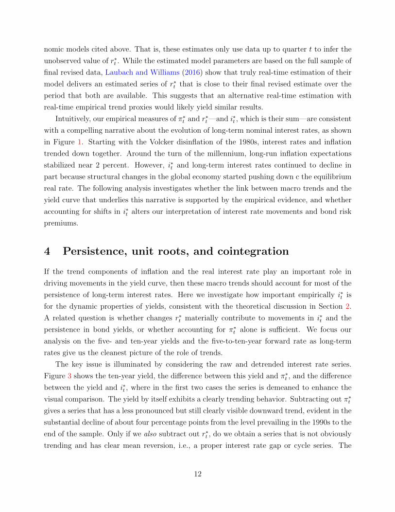
The key issue is illuminated by considering the raw and detrended interest rate series.

Figure 3 shows the ten-year yield, the difference between this yield and π∗t , and the difference

between the yield and i∗t , where in the first two cases the series is demeaned to enhance the

visual comparison. The yield by itself exhibits a clearly trending behavior. Subtracting out π∗t

gives a series that has a less pronounced but still clearly visible downward trend, evident in the

substantial decline of about four percentage points from the level prevailing in the 1990s to the

end of the sample. Only if we also subtract out r∗t , do we obtain a series that is not obviously

trending and has clear mean reversion, i.e., a proper interest rate gap or cycle series. The

12

result is established more formally in the following statistical analysis, which demonstrates

that the persistence in long-term rates is very pronounced, that subtracting i∗t purges most of

this persistence, and that the blue line in Figure 3, y(10y)t − i∗t , is indeed a reasonable measure

of the cycle in long-term bond yields.

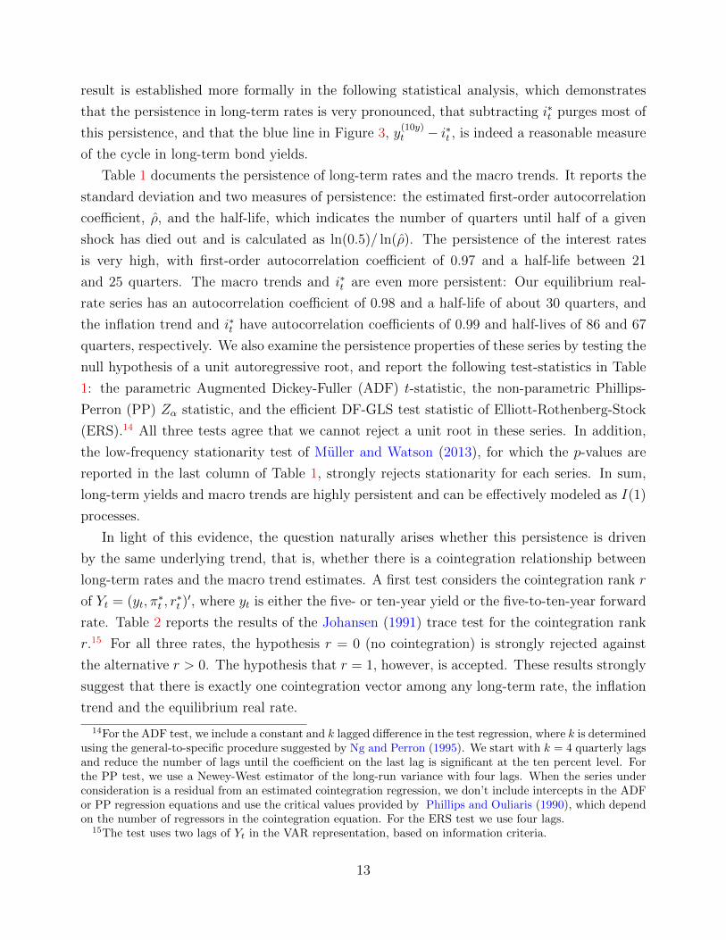
Table 1 documents the persistence of long-term rates and the macro trends. It reports the

standard deviation and two measures of persistence: the estimated first-order autocorrelation

coefficient, ρ, and the half-life, which indicates the number of quarters until half of a given

shock has died out and is calculated as ln(0.5)/ ln(ρ). The persistence of the interest rates

is very high, with first-order autocorrelation coefficient of 0.97 and a half-life between 21

and 25 quarters. The macro trends and i∗t are even more persistent: Our equilibrium real-

rate series has an autocorrelation coefficient of 0.98 and a half-life of about 30 quarters, and

the inflation trend and i∗t have autocorrelation coefficients of 0.99 and half-lives of 86 and 67

quarters, respectively. We also examine the persistence properties of these series by testing the

null hypothesis of a unit autoregressive root, and report the following test-statistics in Table

1: the parametric Augmented Dickey-Fuller (ADF) t-statistic, the non-parametric Phillips-

Perron (PP) Zα statistic, and the efficient DF-GLS test statistic of Elliott-Rothenberg-Stock

(ERS).14 All three tests agree that we cannot reject a unit root in these series. In addition,

the low-frequency stationarity test of Muller and Watson (2013), for which the p-values are

reported in the last column of Table 1, strongly rejects stationarity for each series. In sum,

long-term yields and macro trends are highly persistent and can be effectively modeled as I(1)

processes.

In light of this evidence, the question naturally arises whether this persistence is driven

by the same underlying trend, that is, whether there is a cointegration relationship between

long-term rates and the macro trend estimates. A first test considers the cointegration rank r

of Yt = (yt, π∗t , r∗t )′, where yt is either the five- or ten-year yield or the five-to-ten-year forward

rate. Table 2 reports the results of the Johansen (1991) trace test for the cointegration rank

r.15 For all three rates, the hypothesis r = 0 (no cointegration) is strongly rejected against

the alternative r > 0. The hypothesis that r = 1, however, is accepted. These results strongly

suggest that there is exactly one cointegration vector among any long-term rate, the inflation

trend and the equilibrium real rate.

14For the ADF test, we include a constant and k lagged difference in the test regression, where k is determinedusing the general-to-specific procedure suggested by Ng and Perron (1995). We start with k = 4 quarterly lagsand reduce the number of lags until the coefficient on the last lag is significant at the ten percent level. Forthe PP test, we use a Newey-West estimator of the long-run variance with four lags. When the series underconsideration is a residual from an estimated cointegration regression, we don’t include intercepts in the ADFor PP regression equations and use the critical values provided by Phillips and Ouliaris (1990), which dependon the number of regressors in the cointegration equation. For the ERS test we use four lags.

15The test uses two lags of Yt in the VAR representation, based on information criteria.

13

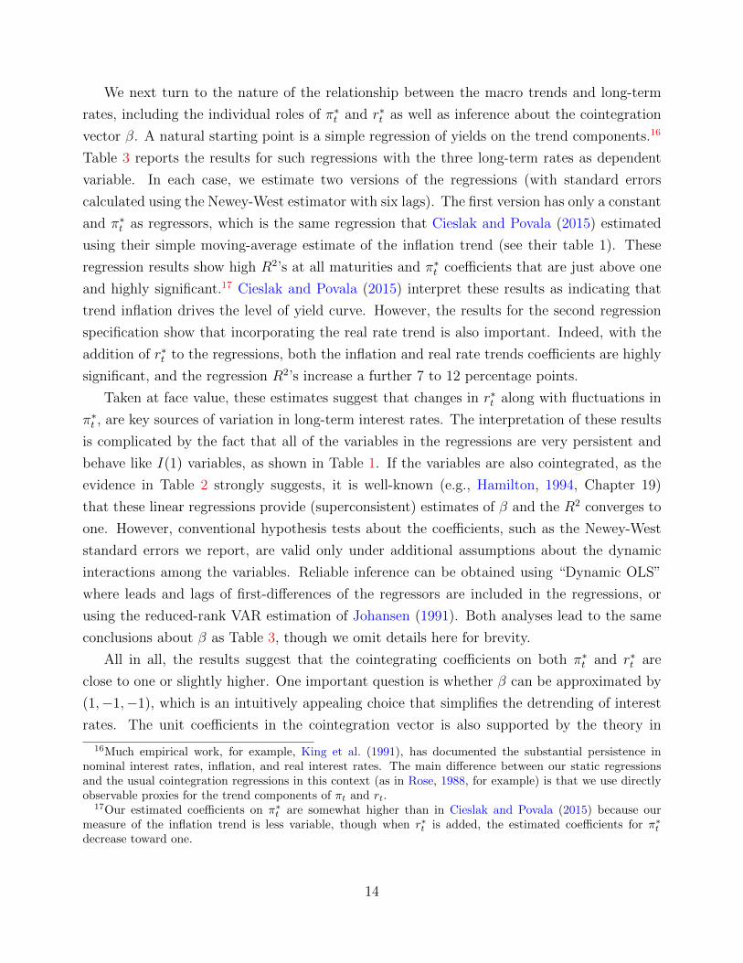
We next turn to the nature of the relationship between the macro trends and long-term

rates, including the individual roles of π∗t and r∗t as well as inference about the cointegration

vector β. A natural starting point is a simple regression of yields on the trend components.16

Table 3 reports the results for such regressions with the three long-term rates as dependent

variable. In each case, we estimate two versions of the regressions (with standard errors

calculated using the Newey-West estimator with six lags). The first version has only a constant

and π∗t as regressors, which is the same regression that Cieslak and Povala (2015) estimated

using their simple moving-average estimate of the inflation trend (see their table 1). These

regression results show high R2’s at all maturities and π∗t coefficients that are just above one

and highly significant.17 Cieslak and Povala (2015) interpret these results as indicating that

trend inflation drives the level of yield curve. However, the results for the second regression

specification show that incorporating the real rate trend is also important. Indeed, with the

addition of r∗t to the regressions, both the inflation and real rate trends coefficients are highly

significant, and the regression R2’s increase a further 7 to 12 percentage points.

Taken at face value, these estimates suggest that changes in r∗t along with fluctuations in

π∗t , are key sources of variation in long-term interest rates. The interpretation of these results

is complicated by the fact that all of the variables in the regressions are very persistent and

behave like I(1) variables, as shown in Table 1. If the variables are also cointegrated, as the

evidence in Table 2 strongly suggests, it is well-known (e.g., Hamilton, 1994, Chapter 19)

that these linear regressions provide (superconsistent) estimates of β and the R2 converges to

one. However, conventional hypothesis tests about the coefficients, such as the Newey-West

standard errors we report, are valid only under additional assumptions about the dynamic

interactions among the variables. Reliable inference can be obtained using “Dynamic OLS”

where leads and lags of first-differences of the regressors are included in the regressions, or

using the reduced-rank VAR estimation of Johansen (1991). Both analyses lead to the same

conclusions about β as Table 3, though we omit details here for brevity.

All in all, the results suggest that the cointegrating coefficients on both π∗t and r∗t are

close to one or slightly higher. One important question is whether β can be approximated by

(1,−1,−1), which is an intuitively appealing choice that simplifies the detrending of interest

rates. The unit coefficients in the cointegration vector is also supported by the theory in

16Much empirical work, for example, King et al. (1991), has documented the substantial persistence innominal interest rates, inflation, and real interest rates. The main difference between our static regressionsand the usual cointegration regressions in this context (as in Rose, 1988, for example) is that we use directlyobservable proxies for the trend components of πt and rt.

17Our estimated coefficients on π∗t are somewhat higher than in Cieslak and Povala (2015) because ourmeasure of the inflation trend is less variable, though when r∗t is added, the estimated coefficients for π∗tdecrease toward one.

14

Section 2, which predicted that yields are affected one-for-one by changes in π∗t and r∗t unless

the macro trends interact with the term premium in such a way as to substantially alter

the effects through expectations. For the long-term forward rate, we can’t reject the null that

β = (1,−1,−1), suggesting that f(5y,10y)t −π∗t−r∗t is not stochastically trending, i.e., stationary.

For the ten-year yield, and particularly for the five-year yield, there is some evidence that the

coefficients on macro trends are above one, but only slightly so. We will show below that

using β = (1,−1,−1) works very well in practice for detrending even the five-year and ten-

year yields. Importantly, the cointegration relationship involves both macro trends, which in

turn implies that a regression of long-term rates on π∗t alone is misspecified and detrending

long-term rates by only π∗t is insufficient.

How much persistent variation in long-term rates is captured by our measures of π∗t and

r∗t ? To address this question we examine the time series properties of detrended long-term

interest rates with one or both of the trend components subtracted out, which are reported in

Table 1. We consider four different ways of detrending interest rates: subtracting out either π∗t

or i∗t or using the residuals from each of the two regressions in Table 3. Several findings stand

out: First, detrending with r∗t as well as π∗t removes substantially more persistence, typically

reducing the half-life by about 40-50%. That is, π∗t is not the only important driver of interest

rate persistence. Second, the detrended series are substantially less variable and less persistent

than the original interest rate series. For example, shocks to the ten-year yield have a half-life

of about 5-1/2 years, whereas shocks to the difference between the ten-year yield and i∗t have a

half-life of just under one year. Clearly, a very substantial share of the persistence in interest

rates is accounted for by i∗t . Finally, although detrending by calculating residuals generally

leads to series that are less persistent than those that are simple differences, if we detrend

with both macro trends than the simple differences do almost as well. In particular for the

forward rate the two series have very similar properties, because the regression coefficients are

already quite close to one. Even detrending with simple differences, i.e., using the cointegrating

residual for β = (1,−1,−1)′, accounts for a large share of the persistence in interest rates, as

long as we use i∗t and not only π∗t .

Unit root tests provide further evidence supporting detrending with both r∗t and π∗t . These

tests show strong evidence against the unit root null for the series that are detrended with

both π∗t and r∗t . By contrast, the unit root null is never rejected at the five percent level for

the original interest rate series or for series that are detrended with just π∗t . When detrending

with both π∗t and r∗t , the ADF and PP tests, as well as the ERS test in the case of the forward

rate, find equally strong or even stronger evidence against a unit root for the simple differences

as for the residuals. For the five- and ten-year yields, the ERS test rejects more strongly for

15

the residuals than for the simple differences, but it still rejects the unit root at the ten-percent

level for simple differences. Finally, the LFST test supports the view that yt− i∗t is stationary

for the ten-year yield and the forward rate, and for the five-year yield, it only marginally

rejects this hypothesis.

These results have implications for the debate about the long-run Fisher effect, which

posits a common trend for inflation and interest rates with a unit coefficient (leaving aside

tax considerations). A sizeable literature has tested this hypothesis with mixed results, often

estimating an inflation coefficient that is significantly larger than one (see Neely and Rapach

(2008)). Our evidence indicates that the series yt−π∗t−r∗t is stationary, which provides support

for a long-run Fisher effect if shifts in the equilibrium real rate are taken into account. The

importance of time variation in r∗t can explain why past research has generally been unable to

find a stable relationship between nominal interest rates and inflation. If yields are regressed

only on inflation or an inflation trend, the regression is misspecified as the residual contains

the omitted trend r∗t . Table 3 shows that the coefficients on π∗t are substantially larger in

regressions when r∗t is excluded, which may explain why it has been difficult to uncover the

Fisher effect.

A final question in this context is whether and how quickly yields respond to shifts in the

trends. To uncover this dynamic response, we estimate a standard error-correction equation

for each of the long-term rate series, using β = (1,−1,−1). First-differenced rates, ∆yt are

regressed on the error-correction term (yt−1 − π∗t−1 − r∗t−1), an intercept, and four lags of ∆yt,

∆π∗t and r∗t . Table 4 shows that the error-correction coefficient is estimated to be significantly

negative, indicating that when long-term are high relative to i∗t they subsequently fall back

toward this trend. That is, yields exhibit strong equilibrium correction. As before, the result

is particularly strong for the forward rate, which has a highly significant coefficient of -0.22, so

a percentage point deviation from the trend is followed by 22 basis points of reversion to the

trend within one quarter. A Wald test shows strong evidence against the hypothesis that the

macro trends do not Granger-cause interest rates. This evidence further supports the view

that interest rates should be jointly modeled with their underlying macro trends, in particular

when it comes to forecasting their future evolution.

5 Predicting excess bond returns

The theoretical discussion and evidence above suggests that knowledge of the macroeconomic

trends underlying yields—and in particular of the current level of yields relative to their trend

i∗t—is important for understanding the evolution of bond yields. We now examine whether

16

such trends can improve predictions of the excess return of long-term bonds over the risk-free

interest rate. Expected excess returns capture bond risk premiums and have long been of

interest in financial economics (Fama and Bliss, 1987).

The excess return for a holding period of h quarters for a bond with maturity n is

rx(n)t,t+h = p

(n−h)t+h − p

(n)t − hy

(h)t = −(n− h)y

(n−h)t+h + ny

(n)t − hy

(h)t .

where p(n)t denotes the log-price of a zero-coupon bond with maturity of n quarters. We predict

the average excess return for all bonds with maturities from two to 15 years, rxt,t+h, for holding

periods of one quarter and four quarters.18 Since Fama and Bliss (1987) and Campbell and

Shiller (1991), it is well-known that the yield curve, and in particular its slope, contains

information useful for predicting future excess returns. The key question is whether the

current yield curve contains all of the information relevant for predicting future returns, that

is, whether the spanning hypothesis holds. Several studies (including Ludvigson and Ng,

2009; Joslin et al., 2014; Cieslak and Povala, 2015) have documented apparent violations

of the spanning hypothesis using various additional predictors. Bauer and Hamilton (2016)

demonstrated that inference in these predictive regressions suffers from serious small-sample

econometric problems arising from highly persistent predictors, and that accounting for these

problems renders most of the proposed predictors insignificant. They found, however, that

the proxy for trend inflation of Cieslak and Povala (2015) was a relatively robust predictor.

Here we investigate whether including both π∗t and r∗t leads to even stronger predictive gains

and rejections of the spanning hypothesis, and whether the reversion to i∗t that was indicated

by our error-correction model explains these predictive gains.

Table 5 reports the results for four different predictive regressions: The first is the common

baseline specification that includes only a constant and the first three principal components

(PCs) of yields.19 The second specification just adds π∗t , and the third specification also

includes r∗t in order to simultaneously capture the effects of both macroeconomic trends. The

fourth specification includes their sum i∗t instead of the two separate macro trends. We report

conventional asymptotically robust standard errors, as well as small-sample p-values for the

macro trends using the parametric bootstrap of Bauer and Hamilton (2016) to avoid the serious

size distortions they document in tests of the spanning hypothesis with persistent predictors.20

18Our long-term bond yields are available only at annual maturities, so we calculate one-quarter returns

with the usual approximation y(n−1)t+1 ≈ y

(n)t+1.

19We scale the PCs such that they correspond to common measures of level, slope and curvature, as in Joslinet al. (2014). For example, the loadings of yields on PC1 add up to one.

20For the conventional estimates, we report White’s heteroskedasticity-robust standard errors for the caseof one-quarter returns and Newey-West standard errors with six lags for the four-quarter returns. For thebootstrap, we simulate 5000 artificial data for yields and predictors under the spanning hypothesis, using

17

In the full sample, the inclusion of an inflation trend increases the predictive power quite

substantially compared to only including yield-curve information: both the inflation trend

and the level of yields (PC1) appear highly significant. This parallels the findings of Cieslak

and Povala (2015). However, adding r∗t to the regressions leads to further impressive gains in

predictive power. For both one-quarter and four-quarter returns, the R2 increases substan-

tially, the coefficients and significance for π∗t and PC1 rise, and the coefficient on r∗t itself is

large and highly significant. Not surprisingly given Figure 1, these results shift in the recent

period as the real-rate trend has gained in importance over time relative to the trend in in-

flation. In the subsample starting in 1985, the inflation trend is not statistically significant

when included on its own according to the small-sample p-values.21 Only with the addition of

the equilibrium real rate, do both trends matter for bond risk premiums; the coefficients on

π∗t and PC1 more than double, the R2 increases substantially, and the coefficients on π∗t and

r∗t are statistically significant. Altogether, our empirical analysis of long-term interest rates

implies that the trend in the real interest rate is as important as, and recently more important

than, the trend in inflation.22

Furthermore, the values of estimated coefficients have a useful interpretation. First, the

similar magnitude of the coefficients on the two individual macro trends suggests that only

their sum matters. Indeed, a Wald test does not reject equality of the coefficients for either

sample or for any of the holding periods. Applying this restriction and including just the

resulting i∗t in the regression provides similarly strong predictive gains. That is, the key to

forecasting excess bond returns is some measure of the overall trend in interest rates. Second,

the coefficient on i∗t has a negative sign and a similar, if slightly larger, absolute magnitude

as the positive coefficient on the yield-curve level (PC1). The intuition is that if the trend

falls then interest rates also fall in response, producing gains for long-term bond holders. For

an annual holding period, a decrease in i∗t by one percentage point predicts an increase in

future excess returns by about 7.5 percentage points. These results document the economic

significance of this mechanism and confirm the influence of trends on yields uncovered in

Section 4.

separate bias-corrected VAR(1) models for yield factors and predictors. The p-values are the fractions ofsimulated samples in which the t-statistics of the macro trends are at least as large (in absolute value) as inthe actual data.

21This result is consistent with Bauer and Hamilton (2016) who in their investigation of the evidence ofCieslak and Povala (2015) also found that in a subsample starting in 1985 the inflation trend is only marginallysignificant.

22In additional, unreported results we have found that the predictive gains from including r∗t stem mainlyfrom the period since the early 2000s when both r∗t and long-term interest rates decreased while long-runinflation expectations where anchored close to two percent. Correspondingly, in samples that exclude thislater period where r∗t variation was most pronounced, only π∗t has significant predictive power.

18

In the presence of persistent predictors, it is generally difficult to interpret the magnitude

of R2 as a measure of predictive accuracy, because even predictors that are irrelevant in

population can substantially increase R2 in small samples (Bauer and Hamilton, 2016). We

can avoid this pitfall by using the bootstrap to generate small-sample distributions of R2 under

the spanning hypothesis and interpret the statistics obtained in the actual data by comparing

them to the quantiles of these distributions. Table 6 reports this comparison for predictive

regressions of annual excess returns for the four specifications we have considered so far, as

well as for two additional ones that will be discussed below. Adding π∗t to the regression

increases R2 by 20 percentage points, but this is only barely higher than the upper end of

the 95%-bootstrap interval, which suggests that under the null hypothesis it would not be too

uncommon to observe an increase in R2 of up to 19 percentage points. In contrast, adding r∗t

increases R2 to 54%, and the increase relative to the yields-only specification of 31 percentage

points is much higher than what is plausible under the null hypothesis. In the post-1985

subsample, the increase in R2 from only adding π∗t is not statistically significant, whereas the

increase of 29 percentage points from adding both trends is strongly significant. Adding just

i∗t instead of the individual macro trends leads to very similar gains in R2 which are highly

significant.

Our findings so far suggest that the predictive power is really contained in detrended yields.

We now consider predictive regressions using yields that are detrended by simply subtracting

the trend, as motivated by the theory in Section 2 and our evidence in Section 4. One way to

assess whether such regressions have similar predictive power is with a hypothesis test of the

restriction that is imposed on a regression with three PCs of yields and i∗t when we instead use

the same linear combinations of detrended yields.23 In the full sample, a Wald test strongly

rejects this restriction, while in the post-1985 sample the null is not rejected. To gauge the

economic significance, we compare regression R2 of restricted and unrestricted regressions in

Table 6. The bottom two rows provide results for predictions using linear combinations of

yields that are detrended either with y(n)t −π∗t or y

(n)t − i∗t . We first note that using yields that

are detrended only by π∗t leads to increases in R2 over the yields-only baseline regression that

are insignificant, while detrending with i∗t leads to much larger increases R2 that are highly

significant. The difference is even more striking in the later subsample that starts in 1985: R2

increases only seven percentage points when detrending with only π∗t but 28 percentage points

when detrending with both π∗t and r∗t . In the full sample, regressions with detrended yields

give somewhat lower R2 than regressions with yields and macro trends, but the sampling

23The unrestricted regression is rxt,t+h = β0 +∑3

i=1 βiw′iYt +β4i

∗t +ut+h, where Yt is a vector with all yields

and wi are the loadings of yields on the i’th PC. The regressors of the restricted regression are w′i(Yt − ιi∗t )

where ι is a vector of ones. Hence the null hypothesis of interest is β4 = −∑3

i=1 βiw′iι.

19

variability of these R2 is large. In the post-1985 subsample, the restricted specifications with

detrended yields achieve similar predictive power as the unrestricted specifications.

In sum, accounting for the persistent components of yields is important for understand-

ing return predictability and estimating bond risk premiums. We find that r∗t has strong

incremental predictive power for bond returns, about on par with the importance of π∗t as a

predictor, suggesting that both macro trends need to be accounted for accurate estimation

of bond risk premiums. The predictive power in the yield curve is fully revealed if they are

detrended, but it is crucial to use i∗t instead of π∗t for the detrending. Finally, little is lost if

detrending is performed by simply taking the difference between yields and i∗t .

While these results are strong evidence against the spanning hypothesis, which is implied

by essentially all asset pricing models (Duffee, 2013), existing macro-finance models can be

readily reconciled with evidence of unspanned predictability. In particular, the addition of very

small bond yield measurement errors—with standard errors of just one or two basis points—

makes it practically impossible to infer all relevant information from observed yields (i.e., to

back out the state variables) (Duffee, 2011b; Cieslak and Povala, 2015; Bauer and Rudebusch,

2017). For the case of macro trends, this problem is particularly acute. There are two level

factors with very similar yield loadings: i∗t on the one hand, and the first principal component

of detrended yields on the other hand.24 Because of measurement error, it is difficult to

attribute any observed level shift to i∗t or to the level of yields relative to i∗t . Therefore, in

practice, yields and macro trends contain separate pieces of important predictive information.

6 Out-of-sample forecasts of interest rates

We now turn to pseudo out-of-sample (OOS) forecasts of long-term interest rates. Despite

many advances in yield curve modeling, the random walk model has proven very hard to beat

when forecasting bond yields, due to the extreme persistence of interest rates (e.g., Duffee,

2013). But our results so far suggest that one might be able to obtain more accurate forecasts

by accounting for the interest rate trends.

In the presence of trends in inflation or the real rate, yields exhibit a “shifting endpoint”

(Kozicki and Tinsley, 2001). Specifically, no-arbitrage theory implies, as evident from (3),

that

y(n)∗t ≡ lim

h→∞Ety

(n)t+h = k(n) + π∗t + r∗t = k(n) + i∗t ,

24The fact that i∗t is a level factor is suggested by the coefficients on π∗t and r∗t in Table 3, and can be seenmost clearly from regressions of yields across all maturities on i∗t . A principal component analysis of detrendedyields, taken either as the residuals of such regressions or as simple differences with i∗t , reveals another levelfactor. Results are omitted for the sake of brevity.

20

where the constant k(n) = CONV (n) + Y TP(n)

captures convexity and the unconditional

mean term premium. This implies that long-horizon forecasts of interest rates that incorporate

knowledge of i∗t should be more accurate than forecasts that ignore it. The forecast method we

propose uses the endpoint y(n)∗t = i∗t based on our macro estimates of π∗t and r∗t . For parsimony,

we set the constant k(n) to zero to avoid introducing additional estimation uncertainty.25 The

other necessary ingredient of our forecast method is a transition path from y(n)t to y

(n)∗t , and we

simply use a smooth, monotonic path from a fitted first-order autoregression for y(n)t − y

(n)∗t .26

Denoting the (recursively) estimated autoregressive coefficient as ρt, the forecasts are thus

constructed as

y(n)t+h = ρht y

(n)t + (1 − ρht )y

(n)∗t . (4)

We denote this forecast method as ME for macro endpoint.27

We compare this model to a driftless random walk as the benchmark, i.e., y(n)t+h = y

(n)t for

all h (denoted as RW ). In addition, we consider shifting-endpoint forecasts that only use the

information in π∗t , in order to assess the importance of incorporating macro estimates of r∗t in

interest-rate forecasts. Specifically, this method uses y(n)∗t = π∗t + µ(n), where the constant is

recursively estimated as the mean of y(n)t −π∗t .

28 We denote these “inflation-only” forecasts as

IO. Finally we include forecasts from a constant-endpoint model, namely a stationary AR(1)

process (AR).

We forecast the five- and ten-year yields and the five-to-ten-year forward rate. At each

point in time, starting in 1976:Q1 (at t = 20) when five years of data are available, we forecast

each interest rate at horizons (h) of 4, 10, 20, 30, and 40 quarters. As indicated above, forecasts

are constructed using a recursive scheme, i.e., using all data available up to the forecast date

to estimate parameters.29 Table 7 reports the root-mean-squared errors (RMSEs) and mean-

absolute errors (MAEs), in percentage points. We also calculate p-values for tests of equal

25We have found that including an estimated constant generally worsens forecast performance.26In a fully-specified model with yields and macro trends—even in the simple no-arbitrage model in Appendix

A—the speed of mean reversion to y(n)∗t depends on the importance of the different cyclical factors. Our simple

method corresponds to the special case where all cyclical factors have the same speed of mean reversion.Notably, the exact speed of mean reversion affects mainly short-horizon forecasts and is inconsequential forour main results.

27Note that this approach could easily be extended to provide joint forecasts of the entire yield curve, forexample, extending Diebold and Li (2006) and Dijk et al. (2014) by simply forecasting the Nelson-Siegel levelfactor in the same fashion.

28We found that forecasts which assume that this constant is zero are much less accurate, which is unsur-prising since they counterfactually assume that k(n) + r∗t = 0.

29A rolling scheme, which uses only a fixed number of observations for parameter estimation, allows foran easier asymptotic justification of tests for predictive ability (Giacomini and White, 2006) but requires aspecific choice of the window length. We have also obtained forecasts with such a scheme, using a variety ofdifferent window lengths, and found equally strong forecast gains for model ME as using a recursive scheme.

21

finite-sample forecast accuracy using the approach of Diebold and Mariano (1995) (DM).30

We calculate these DM p-values, using standard normal critical values, for one-sided tests of

the null hypothesis that our proposed model ME does not improve upon the RW and IO

forecasts. We find that model ME achieves substantial and statistically significant gains in

forecast accuracy at long horizons. Such gains are evident for both RMSEs and MAEs, but

are larger and more strongly significant for absolute-error loss. For example, when forecasting

the ten-year yield five years ahead, model ME lowers the RMSE by over 25% relative to RW,

an improvement that is significant at the five-percent level, while the MAE drops by more

than 40% and is significant at the one percent level. Model ME also improves upon IO by a

magnitude that is typically large and statistically significant.31

These results document that at long horizons one can significantly improve upon random

walk interest rate forecasts by incorporating macroeconomic information on i∗t , the underlying

trend in interest rates. In contrast to the random walk forecast, which simply assumes all

changes are permanent, using estimates of i∗t captures the underlying source and share of the

highly persistent changes in interest rates with large benefits for forecast accuracy. Further-

more, it is clearly important to incorporate macro estimates of r∗t in addition to information

on π∗t , because this substantially improves the accuracy of the estimated shifting endpoint in

yields.32 Earlier research by Dijk et al. (2014) found that when forecasting interest rates it is

beneficial to link long-run projections of interest rates to long-run expectations of inflation,

but this ignores the advantages of recognizing the time variation in r∗t . In addition, our results

also show that there is no need to estimate a constant or to scale the endpoint (as in Dijk

et al., 2014) once a macro-based estimate of r∗t is incorporated into i∗t .

Finally, we compare the accuracy of our statistical models to that of professional forecasters

for predicting the ten-year yield. Since 1988, the Blue Chip Financial Forecasts (BC ) survey

has asked its respondents for long-range forecasts twice a year. The respondents provide

their average expectations of the target variable for each of the upcoming five calendar years

and for the subsequent five-year period—we will focus on the five annual forecast horizons.33

30Following common use, we construct the DM test with a rectangular window for the long-run variance andthe small-sample adjustment of Harvey et al. (1997). Monte Carlo evidence in Clark and McCracken (2013)indicates that this test has good size in finite samples. However, for very long forecast horizons the long-run variance is estimated with considerable uncertainty as in those cases there are only few non-overlappingobservations in our sample.

31We have found in additional, unreported analysis—using plots of differences in cumulative sums of forecasterrors over time—that the forecast gains of ME are not driven by certain unusual sub-periods, but instead area consistent pattern over most of our sample period.

32The source of the forecast gains of model ME relative to IO is the lower level of r∗t . Model IO uses ineffect the (recursively estimated) mean of the difference between yields and π∗t as its estimate of r∗t , whichover most of the sample period was too high.

33For survey dates in the fourth quarter, one calendar year is typically skipped. We use the exact years from

22

We match the available information sets by using only data up to the quarter preceding

the survey date for our model-based forecasts, and we exactly match the forecast horizons

with the BC forecasts by taking averages of model-based forecasts over the relevant calendar

years. The sample includes 46 forecast dates from March 1988 to December 2010. Table

8 shows the RMSEs and MAEs of the survey forecasts and the four model-based forecasts.

Shifting-endpoint forecasts based on i∗t improve substantially over both RW and BC forecasts

in this sample. The gains relative to RW are strongly significant for horizons beyond the first

calendar year, and the gains relative to BC are significant at the five- or ten-percent level. The

reason for the poor performance of the survey forecasts is that they consistently over-predict

future yields at these long horizons: The difference between long-range survey forecasts of

the ten-year yield and our (survey-based) estimate of π∗t is much larger than our macro-based

estimate of r∗t (results not shown). Other studies have documented the poor performance of

survey forecasts of interest rates (e.g., Dijk et al., 2014), which contrasts with the very good

performance of survey-based inflation forecasts(Ang et al., 2007; Faust and Wright, 2013).

Our results suggest that the underlying reason for this poor performance is that professional

forecasters have in the past overestimated the trend component in interest rates.

7 The term premium in long-term yields

The term premium is defined as the difference between holding an n-period bond to maturity

or facing a sequence of one-period rates over the same period:

TP(n)t = y

(n)t − 1

n

n−1∑j=0

Ety(1)t+j.

Estimation of the term premium requires expectations of future short-term rates, which are

commonly obtained from a stationary VAR that underlies either a no-arbitrage model or a

simple factor model. However, our results suggest that the stationarity assumption is prob-

lematic for long-horizon forecasts. We now investigate how it affects term premium estimates

if we instead allow for a trend component in interest rates based on equation (3) and the

underlying macro trends.

Decompositions of long-term interest rates into short-rate expectations and term premiums

are commonly obtained from a variety of dynamic models, usually with a factor structure

for yields and often with no-arbitrage restrictions on the factor loadings. Our approach will

closely follow Cochrane (2007), who estimated simple VAR model for interest rates without no-

the actual survey to line up our forecasts.

23

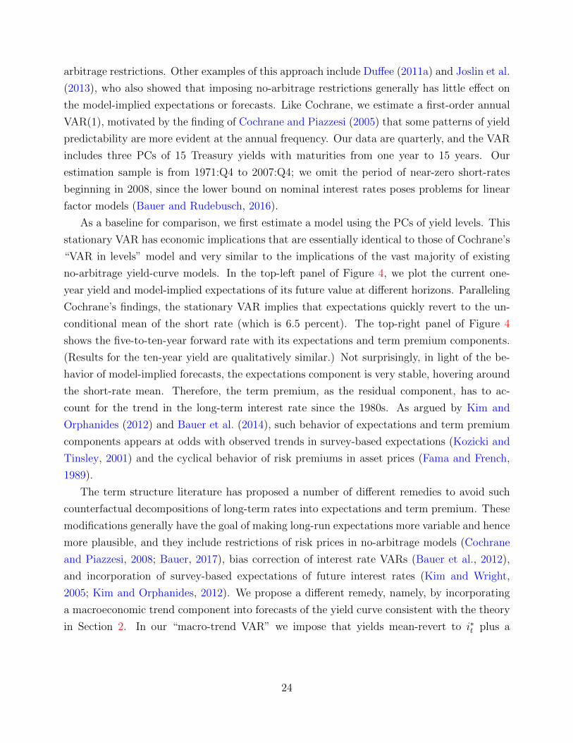
arbitrage restrictions. Other examples of this approach include Duffee (2011a) and Joslin et al.

(2013), who also showed that imposing no-arbitrage restrictions generally has little effect on

the model-implied expectations or forecasts. Like Cochrane, we estimate a first-order annual

VAR(1), motivated by the finding of Cochrane and Piazzesi (2005) that some patterns of yield

predictability are more evident at the annual frequency. Our data are quarterly, and the VAR

includes three PCs of 15 Treasury yields with maturities from one year to 15 years. Our

estimation sample is from 1971:Q4 to 2007:Q4; we omit the period of near-zero short-rates

beginning in 2008, since the lower bound on nominal interest rates poses problems for linear

factor models (Bauer and Rudebusch, 2016).

As a baseline for comparison, we first estimate a model using the PCs of yield levels. This

stationary VAR has economic implications that are essentially identical to those of Cochrane’s

“VAR in levels” model and very similar to the implications of the vast majority of existing

no-arbitrage yield-curve models. In the top-left panel of Figure 4, we plot the current one-

year yield and model-implied expectations of its future value at different horizons. Paralleling

Cochrane’s findings, the stationary VAR implies that expectations quickly revert to the un-

conditional mean of the short rate (which is 6.5 percent). The top-right panel of Figure 4

shows the five-to-ten-year forward rate with its expectations and term premium components.

(Results for the ten-year yield are qualitatively similar.) Not surprisingly, in light of the be-

havior of model-implied forecasts, the expectations component is very stable, hovering around

the short-rate mean. Therefore, the term premium, as the residual component, has to ac-

count for the trend in the long-term interest rate since the 1980s. As argued by Kim and

Orphanides (2012) and Bauer et al. (2014), such behavior of expectations and term premium

components appears at odds with observed trends in survey-based expectations (Kozicki and

Tinsley, 2001) and the cyclical behavior of risk premiums in asset prices (Fama and French,

1989).

The term structure literature has proposed a number of different remedies to avoid such

counterfactual decompositions of long-term rates into expectations and term premium. These

modifications generally have the goal of making long-run expectations more variable and hence

more plausible, and they include restrictions of risk prices in no-arbitrage models (Cochrane

and Piazzesi, 2008; Bauer, 2017), bias correction of interest rate VARs (Bauer et al., 2012),

and incorporation of survey-based expectations of future interest rates (Kim and Wright,

2005; Kim and Orphanides, 2012). We propose a different remedy, namely, by incorporating

a macroeconomic trend component into forecasts of the yield curve consistent with the theory

in Section 2. In our “macro-trend VAR” we impose that yields mean-revert to i∗t plus a

24

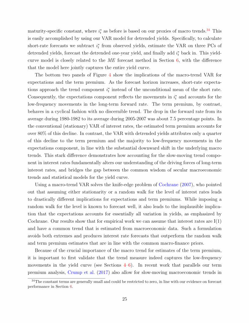
maturity-specific constant, where i∗t as before is based on our proxies of macro trends.34 This

is easily accomplished by using our VAR model for detrended yields. Specifically, to calculate

short-rate forecasts we subtract i∗t from observed yields, estimate the VAR on three PCs of

detrended yields, forecast the detrended one-year yield, and finally add i∗t back in. This yield-

curve model is closely related to the ME forecast method in Section 6, with the difference

that the model here jointly captures the entire yield curve.

The bottom two panels of Figure 4 show the implications of the macro-trend VAR for

expectations and the term premium. As the forecast horizon increases, short-rate expecta-

tions approach the trend component i∗t instead of the unconditional mean of the short rate.

Consequently, the expectations component reflects the movements in i∗t and accounts for the

low-frequency movements in the long-term forward rate. The term premium, by contrast,

behaves in a cyclical fashion with no discernible trend. The drop in the forward rate from its

average during 1980-1982 to its average during 2005-2007 was about 7.5 percentage points. In

the conventional (stationary) VAR of interest rates, the estimated term premium accounts for

over 80% of this decline. In contrast, the VAR with detrended yields attributes only a quarter

of this decline to the term premium and the majority to low-frequency movements in the

expectations component, in line with the substantial downward shift in the underlying macro

trends. This stark difference demonstrates how accounting for the slow-moving trend compo-

nent in interest rates fundamentally alters our understanding of the driving forces of long-term

interest rates, and bridges the gap between the common wisdom of secular macroeconomic

trends and statistical models for the yield curve.

Using a macro-trend VAR solves the knife-edge problem of Cochrane (2007), who pointed

out that assuming either stationarity or a random walk for the level of interest rates leads

to drastically different implications for expectations and term premiums. While imposing a

random walk for the level is known to forecast well, it also leads to the implausible implica-

tion that the expectations accounts for essentially all variation in yields, as emphasized by

Cochrane. Our results show that for empirical work we can assume that interest rates are I(1)

and have a common trend that is estimated from macroeconomic data. Such a formulation

avoids both extremes and produces interest rate forecasts that outperform the random walk

and term premium estimates that are in line with the common macro-finance priors.

Because of the crucial importance of the macro trend for estimates of the term premium,

it is important to first validate that the trend measure indeed captures the low-frequency

movements in the yield curve (see Sections 4–6). In recent work that parallels our term

premium analysis, Crump et al. (2017) also allow for slow-moving macroeconomic trends in

34The constant terms are generally small and could be restricted to zero, in line with our evidence on forecastperformance in Section 6.

25

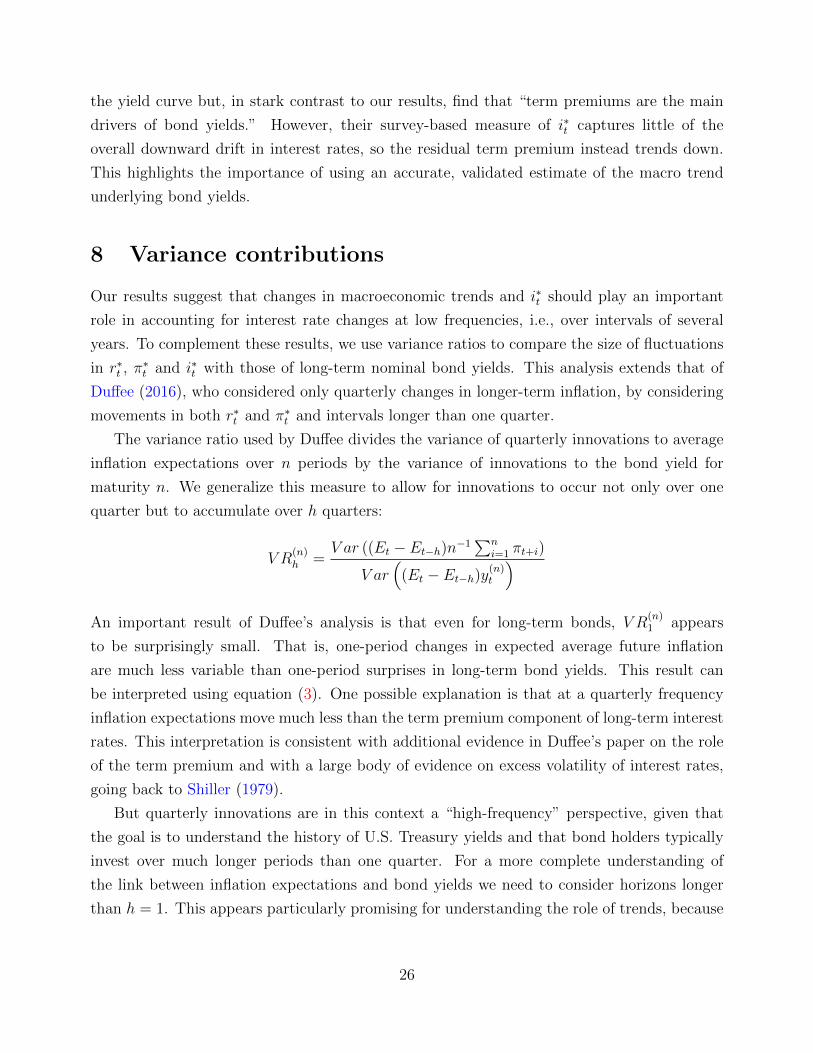
the yield curve but, in stark contrast to our results, find that “term premiums are the main

drivers of bond yields.” However, their survey-based measure of i∗t captures little of the

overall downward drift in interest rates, so the residual term premium instead trends down.

This highlights the importance of using an accurate, validated estimate of the macro trend

underlying bond yields.

8 Variance contributions

Our results suggest that changes in macroeconomic trends and i∗t should play an important

role in accounting for interest rate changes at low frequencies, i.e., over intervals of several

years. To complement these results, we use variance ratios to compare the size of fluctuations

in r∗t , π∗t and i∗t with those of long-term nominal bond yields. This analysis extends that of

Duffee (2016), who considered only quarterly changes in longer-term inflation, by considering

movements in both r∗t and π∗t and intervals longer than one quarter.

The variance ratio used by Duffee divides the variance of quarterly innovations to average

inflation expectations over n periods by the variance of innovations to the bond yield for

maturity n. We generalize this measure to allow for innovations to occur not only over one

quarter but to accumulate over h quarters:

V R(n)h =

V ar ((Et − Et−h)n−1∑n

i=1 πt+i)

V ar(

(Et − Et−h)y(n)t

)An important result of Duffee’s analysis is that even for long-term bonds, V R

(n)1 appears

to be surprisingly small. That is, one-period changes in expected average future inflation

are much less variable than one-period surprises in long-term bond yields. This result can

be interpreted using equation (3). One possible explanation is that at a quarterly frequency

inflation expectations move much less than the term premium component of long-term interest

rates. This interpretation is consistent with additional evidence in Duffee’s paper on the role

of the term premium and with a large body of evidence on excess volatility of interest rates,

going back to Shiller (1979).

But quarterly innovations are in this context a “high-frequency” perspective, given that

the goal is to understand the history of U.S. Treasury yields and that bond holders typically

invest over much longer periods than one quarter. For a more complete understanding of

the link between inflation expectations and bond yields we need to consider horizons longer

than h = 1. This appears particularly promising for understanding the role of trends, because

26

limh→∞

V R(n)h is only affected by changes in trend components.35 That is, if the inflation trend

is an important determinant for yields we should see a clear tendency for variance ratios to

rise with h. Of course, the variance ratios become harder to estimate with increasing h as

the overlap of observations increases and one loses degrees of freedom and precision. Despite

this estimation uncertainty, the profile of variance ratios across horizons can provide evidence

about the role of low-frequency movements in macro trends for interest rate dynamics.

Estimation of the these variance ratios requires expectations of inflation and interest rates.

Like Duffee, we consider survey-based inflation expectations (in our measure of π∗t ) and mar-

tingale interest rate forecasts. But, instead of modeling the inflation process, we approximate

inflation news by the change in π∗t . This allows us to calculate the simplified variance ratio

V R(n)

h =V ar (∆hπ

∗t )

V ar(

∆hy(n)t

) , ∆hzt = zt − zt−h.

For any given n and h, V R(n)

h differs from V R(n)h but, these differences are likely to be small

for longer horizons h since

limh→∞

V R(n)

h = limh→∞

V R(n)h =

V ar(∆π∗t )

V ar(∆i∗t ).

Thus, for low-frequency movements, the two inflation variance ratios are asymptotically iden-

tical and capture the importance of the inflation trend for the overall yield trend.

Figure 5 shows estimates of V R(n)

h for changes from one quarter to h = 40 quarters in

the five-year yield, the ten-year yield, and the 5-to-10-year forward rate. Similarly, we also

calculate these variance ratios for the contribution of changes in the real-rate trend, r∗t , and in

the overall trend component i∗t = π∗t + r∗t , simply by replacing the variance in the numerator

of V R(n)

h .

For the inflation trend, we find that one-quarter variance ratios are around 0.1. This

result is consistent with Duffee’s findings and suggests that changes in the inflation trend play

a small role for variation in yields at the quarterly frequency. At lower frequencies, however,

the relative variability of the inflation trend increases. The point estimates of the π∗t -variance

ratio quickly rise with the horizon, and for h = 40 reach a magnitude of around 0.3. This

shows that inflation expectations are of substantial importance for movements in bond yields

once we shift the focus from month-to-month or quarter-to-quarter variation and look at lower

frequencies changes over several years.

35This statement assumes that the term premium is stationary, an assumption generally made in yield-curvemodeling and supported by our findings in Section 4.

27

The variance ratio for changes in the real-rate trend, i.e., V ar(∆hr∗t )/V ar(∆hyt), is much

lower than for inflation, remaining below 0.1 even at long horizons. This is unsurprising in

light of Figure 1, which shows that over the full sample the movements in r∗t were substantially

less pronounced than movements in long-term interest rates and the inflation trend. Of course,

this perspective of unconditional variances should not be taken to conclude that changes in

the equilibrium real rate are unimportant for interest rate dynamics, given the ample evidence

in Sections 4– 6 of the crucial role of r∗t for modeling and forecasting interest rates. From a

conditional perspective, changes in r∗t have become very important later in our sample, which

is not evident in full-sample moments.

To assess the overall importance of the trend components in interest rates, we consider

variance ratios for i∗t , i.e., V ar(∆hi∗t )/V ar(∆hyt). Confidence intervals are obtained using

the asymptotic distribution of the sample variances and the delta method. To account for

persistence in conditional variances, Newey-West estimates of long-run variances are used.36

Figure 5 shows that while the sampling uncertainty around the variance ratios for changes in

i∗t is substantial we can be reasonably confident that these variance ratios increase from below

0.15 to a range of around 0.25 to 0.4, depending on the maturity of the interest rate. The

highest levels are reached for the 5-to-10-year forward rate—the confidence interval at h = 40

extends from about 0.3 to 0.4—which is consistent with the notion that distant forward rates

are more strongly affected by the trend components.

While in theory we have limh→∞

V ar(∆hi∗t )/V ar(∆hyt) = 1, our estimates top out around 0.4.

While this might be due to the fact that we are simply not capturing the trend component

with sufficient accuracy, we have provided ample evidence that our trend proxies are closely

linked to the yield curve. Hence it appears that the cyclical components of inflation and the

real rate together with movements in the term premium still make substantial contributions

to interest rate movements at frequencies corresponding to ten-year changes.

To shed further light on this topic, it is useful to consider not only the direct contribution

of changes in the trend to changes in interest rates, but also the indirect contribution due to

comovement of trend and cycle components. In Table 9, we report the variances of changes in

interest rates, in the trend component i∗t , and in the cycle components yt − i∗t . The variance

of yield changes can be decomposed as follows:

V ar(∆hyt) = V ar(∆hi∗t ) + V ar(∆hyt − ∆hi

∗t ) + 2Cov(∆hi

∗t ,∆hyt − ∆hi

∗t ).

36We use 12 quarterly lags for all long-run variance estimates as indicated by the automatic lag selectionprocedure of Newey and West. These confidence intervals may understate the true sampling variability due tothe small number of non-overlapping observations, which decreases the reliability of the asymptotic approxi-mations.

28

The first term captures the direct contribution of trends, whereas the last term captures the

their indirect contribution to movements in yields. Table 9 reports all three components. In

the data, the contribution of the covariance is small at short horizons, but substantial at long

horizons. The two last rightmost columns of Table 9 report the same variance ratio shown

in Figure 5 along with a ratio that also includes the covariance contribution—the indirect

effects—in the numerator. This second ratio rises to over 0.7 with horizon, which suggests

that the cycle component by itself accounts for less than 30% of the variance of interest rate

changes at low frequencies. These estimates strengthen our finding that changes in macro

trends play an important role in low-frequency movements in interest rates.

9 Conclusion

We have provided much compelling new evidence from a variety of perspectives that interest

rates and bond risk premiums are substantially driven by time variation in the trend in inflation

and the equilibrium real rate of interest. Our results demonstrate that the links between

macroeconomic trends and the yield curve are quantitatively important, and that accounting

for these time-varying trend components is crucial for understanding and forecasting long-term

interest rates and bond returns. Our paper therefore provides strong support for building yield

curve models that allow for slow-moving changes in the long-run means of nominal and real

interest rates and inflation instead of the stationary dynamic specifications with constant

means that are ubiquitous.37

Our analysis established the links between macroeconomic trends and yields by taking

as data the off-the-shelf estimates of the trends from surveys and models. While this is

a productive exercise, future research should jointly estimate macro trends and yield curve

dynamics. One of the many benefits of such analysis would be the ability to investigate the

role of model and estimation uncertainty. Another important future research avenue is to to

consider potential changes over time in the variability of the trends. For example, it is well

known (e.g., Stock and Watson, 2007) that the trend component of inflation was much more

variable in the 1970s and 1980s than in more recent decades. This raises the question how our

(mostly unconditional) results are affected by taking a conditional perspective. Furthermore,

this suggests that incorporating not only macroeconomic trends but also stochastic volatility

in these trend components will be useful for term structure modeling.

37Conversely, our evidence suggests that long-term yields contain relevant information about r∗t and shouldtherefore be included in the estimation, and some recent studies take a first step in this direction (Johannsenand Mertens, 2016; Del Negro et al., 2017).

29

References

Adrian, Tobias, Richard K. Crump, and Emanuel Moench (2013) “Pricing the Term Structure

with Linear Regressions,” Journal of Financial Economics, Vol. 110, pp. 110–138.

Ang, Andrew, Geert Bekaert, and Min Wei (2007) “Do macro variables, asset markets, or

surveys forecast ination better?” Journal of Monetary Economics, Vol. 54, pp. 1163–1212.

Ang, Andrew and Monika Piazzesi (2003) “A No-Arbitrage Vector Autoregression of Term

Structure Dynamics with Macroeconomic and Latent Variables,” Journal of Monetary Eco-

nomics, Vol. 50, pp. 745–787.

Bansal, Ravi and Ivan Shaliastovich (2013) “A Long-Run Risks Explanation of Predictability

Puzzles in Bond and Currency Markets,” Review of Financial Studies, Vol. 26, pp. 1–33.

Bauer, Michael D. (2017) “Restrictions on Risk Prices in Dynamic Term Structure Models,”

Journal of Business & Economic Statistics, in press.

Bauer, Michael D. and James D. Hamilton (2016) “Robust Bond Risk Premia,” Working

Paper 2015-15, Federal Reserve Bank of San Francisco.

Bauer, Michael D. and Glenn D. Rudebusch (2016) “Monetary Policy Expectations at the

Zero Lower Bound,” Journal of Money, Credit and Banking, Vol. 48, pp. 1439–1465.

(2017) “Resolving the Spanning Puzzle in Macro-Finance Term Structure Models,”

Review of Finance, Vol. 21, pp. 511–553.

Bauer, Michael D., Glenn D. Rudebusch, and Jing Cynthia Wu (2012) “Correcting Estimation

Bias in Dynamic Term Structure Models,” Journal of Business & Economic Statistics, Vol.

30, pp. 454–467.

(2014) “Term Premia and Inflation Uncertainty: Empirical Evidence from an Inter-

national Panel Dataset: Comment,” American Economic Review, Vol. 104, pp. 1–16.

Bikbov, Ruslan and Mikhail Chernov (2010) “No-Arbitrage Macroeconomic Determinants of

the Yield Curve,” Journal of Econometrics, Vol. 159, pp. 166–182.

Brayton, Flint and Peter Tinsley (1996) “A Guide to FRB/US: A Macroeconomic Model of

the United States,” Finance and Economics Discussion Series 1996-42, Board of Governors

of the Federal Reserve System.

30

Brooks, Jordan and Tobias J. Moskowitz (2017) “Yield Curve Premia,” July, unpublished

manuscript.

Campbell, John Y, Andrew Wen-Chuan Lo, and Archie Craig MacKinlay (1997) The Econo-

metrics of Financial Markets: Princeton University Press.

Campbell, John Y and Pierre Perron (1991) “Pitfalls and opportunities: what macroe-

conomists should know about unit roots,” NBER macroeconomics annual, Vol. 6, pp. 141–

201.

Campbell, John Y. and Robert J. Shiller (1991) “Yield Spreads and Interest Rate Movements:

A Bird’s Eye View,” Review of Economic Studies, Vol. 58, pp. 495–514.

Carvalho, Carlos, Andrea Ferrero, and Fernanda Nechio (2016) “Demographics and real in-

terest rates: inspecting the mechanism,” European Economic Review, Vol. 88, pp. 208–226.

Christensen, Jens H. E., Jose A. Lopez, and Glenn D. Rudebusch (2010) “Inflation Expecta-

tions and Risk Premiums in an Arbitrage-Free Model of Nominal and Real Bond Yields,”

Journal of Money, Credit and Banking, Vol. 42, pp. 143–178.

Christensen, Jens H.E. and Glenn D. Rudebusch (2017) “A New Normal for Interest Rates?

Evidence from Inflation-Indexed Debt,” Working Paper 2017-07, Federal Reserve Bank of

San Francisco.

Cieslak, Anna and Pavol Povala (2015) “Expected Returns in Treasury Bonds,” Review of

Financial Studies, Vol. 28, pp. 2859–2901.

Clark, Todd E and Sharon Kozicki (2005) “Estimating equilibrium real interest rates in real

time,” The North American Journal of Economics and Finance, Vol. 16, pp. 395–413.

Clark, Todd and Michael McCracken (2013) “Advances in Forecast Evaluation,” in Graham

Elliott and Allan Timmermann eds. Handbook of Economic Forecasting, Vol. 2, Part B:

Elsevier, pp. 1107 – 1201.

Cochrane, John (2007) “Commentary on “Macroeconomic implications of changes in the term

premium”,” Federal Reserve Bank of St. Louis Review, pp. 271–282.

Cochrane, John H. and Monika Piazzesi (2005) “Bond Risk Premia,” American Economic

Review, Vol. 95, pp. 138–160.

(2008) “Decomposing the Yield Curve,” unpublished manuscript, Chicago Booth

School of Business.

31

Crump, Richard, Stefano Eusepi, and Emanuel Moench (2017) “The term structure of expec-

tations and bond yields,”Technical report, Federal Reserve Bank of New York.

Curdia, Vasco, Andrea Ferrero, Ging Cee Ng, and Andrea Tambalotti (2015) “Has US mon-

etary policy tracked the efficient interest rate?” Journal of Monetary Economics, Vol. 70,

pp. 72–83.

Del Negro, Marco, Domenica Giannone, Marc Giannoni, and Andrea Tambalotti (2017)

“Safety, liquidity, and the natural rate of interest,” March, Brookings Papers on Economic

Activity, Conference Draft.

Dewachter, Hans and Leonardo Iania (2011) “An Extended Macro-Finance Model with Fi-

nancial Factors.,” Journal of Financial & Quantitative Analysis, Vol. 46.

Dewachter, Hans and Marco Lyrio (2006) “Macro Factors and the Term Structure of Interest

Rates,” Journal of Money, Credit and Banking, Vol. 38, pp. 119–140.

Diebold, Francis X. and Canlin Li (2006) “Forecasting the term structure of government bond

yields,” Journal of Econometrics, Vol. 130, pp. 337–364.

Diebold, Francis X. and Robert S. Mariano (1995) “Comparing Predictive Accuracy,” Journal

of Business & Economic Statistics, Vol. 13, pp. 253–263.

Diebold, Francis X., Glenn D. Rudebusch, and S. Boragan Aruoba (2006) “The Macroeconomy

and the Yield Curve: A Dynamic Latent Factor Approach,” Journal of Econometrics, Vol.

131, pp. 309–338.

van Dijk, Dick, Siem Jan Koopman, Michel Wel, and Jonathan H Wright (2014) “Forecasting

interest rates with shifting endpoints,” Journal of Applied Econometrics, Vol. 29, pp. 693–

712.

Duffee, Gregory R. (2002) “Term Premia and Interest Rate Forecasts in Affine Models,”

Journal of Finance, Vol. 57, pp. 405–443.

(2011a) “Forecasting with the Term Structure: the Role of No-Arbitrage,” Working

Paper January, Johns Hopkins University.

(2011b) “Information In (and Not In) the Term Structure,” Review of Financial

Studies, Vol. 24, pp. 2895–2934.

(2013) “Forecasting Interest Rates,” in Graham Elliott and Allan Timmermann eds.

Handbook of Economic Forecasting, Vol. 2, Part A: Elsevier, pp. 385–426.

32

(2016) “Expected inflation and other determinants of Treasury yields,” July, unpub-

lished manuscript.

Dybvig, P.H., J.E. Ingersoll Jr, and S.A. Ross (1996) “Long forward and zero-coupon rates

can never fall,” Journal of Business, Vol. 69, pp. 1–25.

Evans, Martin D. and Karen K. Lewis (1995) “Do Expected Shifts in Inflation Affect Estimates

of the Long-Run Fisher Relation?” Journal of Finance, Vol. 50, pp. 225–253.

Fama, Eugene F (2006) “The behavior of interest rates,” The Review of Financial Studies,

Vol. 19, pp. 359–379.

Fama, Eugene F. and Robert R. Bliss (1987) “The Information in Long-Maturity Forward

Rates,” American Economic Review, Vol. 77, pp. 680–692.

Fama, Eugene F and Kenneth R French (1989) “Business conditions and expected returns on

stocks and bonds,” Journal of financial economics, Vol. 25, pp. 23–49.

Faust, Jon and Jonathan H. Wright (2013) “Forecasting Inflation,” in G. Elliott and A. Tim-

merman eds. Handbook of Economic Forecasting, Vol. 2, Part A: North-Holland, pp. 2–56.

Garg, Ashish and Michele Mazzoleni (2017) “The Natural Rate of Interest and Bond Returns,”

April, unpublished manuscript.

Giacomini, Raffaella and Halbert White (2006) “Tests of conditional predictive ability,” Econo-

metrica, Vol. 74, pp. 1545–1578.

Gurkaynak, Refet S., Brian Sack, and Jonathan H. Wright (2007) “The U.S. Treasury yield

curve: 1961 to the present,” Journal of Monetary Economics, Vol. 54, pp. 2291–2304.

Gurkaynak, Refet S. and Jonathan H. Wright (2012) “Macroeconomics and the Term Struc-

ture,” Journal of Economic Literature, Vol. 50, pp. 331–367.

Hamilton, James D. (1994) Time Series Analysis: Princeton University Press.

Hamilton, James D., Ethan S. Harris, Jan Hatzius, and Kenneth D. West (2016) “The Equi-

librium Real Funds Rate: Past, Present, and Future,” IMF Economic Review, Vol. 64, pp.

660–707.

Harvey, David, Stephen Leybourne, and Paul Newbold (1997) “Testing the equality of pre-

diction mean squared errors,” International Journal of Forecasting, Vol. 13, pp. 281–291.

33

Holston, Kathryn, Thomas Laubach, and John C Williams (2017) “Measuring the natural rate

of interest: International trends and determinants,” Journal of International Economics,

Vol. 108, pp. S59–S75.

Hordahl, Peter, Oreste Tristani, and David Vestin (2006) “A Joint Econometric Model of

Macroeconomic and Term-Structure Dynamics,” Journal of Econometrics, Vol. 131, pp.

405–444.

Hyslop, Dean R and Guido W Imbens (2001) “Bias from classical and other forms of mea-

surement error,” Journal of Business & Economic Statistics, Vol. 19, pp. 475–481.

Johannsen, Benjamin K and Elmar Mertens (2016) “A Time Series Model of Interest Rates

With the Effective Lower Bound,” Finance and Economics Discussion Series 2016-033,

Board of Governors of the Federal Reserve System.

Johansen, Søren (1991) “Estimation and hypothesis testing of cointegration vectors in Gaus-

sian vector autoregressive models,” Econometrica, pp. 1551–1580.

Jorgensen, Kasper (2017) “How Learning from Macroeconomic Experiences Shapes the Yield

Curve,” October, unpublished manuscript.

Joslin, Scott, Anh Le, and Kenneth J. Singleton (2013) “Why Gaussian Macro-Finance Term

Structure Models Are (Nearly) Unconstrained Factor-VARs,” Journal of Financial Eco-

nomics, Vol. 109, pp. 604–622.

Joslin, Scott, Marcel Priebsch, and Kenneth J. Singleton (2014) “Risk Premiums in Dynamic

Term Structure Models with Unspanned Macro Risks,” Journal of Finance, Vol. 69, pp.

1197–1233.

Kiley, Michael T. (2015) “What Can the Data Tell Us About the Equilibrium Real Interest

Rate,” FEDS Working Paper 2015-077, Board of Governors of the Federal Reserve System.

Kim, Don H. and Athanasios Orphanides (2012) “Term Structure Estimation with Survey

Data on Interest Rate Forecasts,” Journal of Financial and Quantitative Analysis, Vol. 47,

pp. 241–272.

Kim, Don H. and Jonathan H. Wright (2005) “An arbitrage-free three-factor term structure

model and the recent behavior of long-term yields and distant-horizon forward rates,” Fi-

nance and Economics Discussion Series 2005-33, Federal Reserve Board of Governors.

34

King, Robert G., Charles I. Plosser, James H. Stock, and Mark W. Watson (1991) “Stochastic

Trends and Economic Fluctuations,” The American Economic Review, Vol. 81, pp. 819–840.

Kozicki, S. and P.A. Tinsley (2001) “Shifting endpoints in the term structure of interest rates,”

Journal of Monetary Economics, Vol. 47, pp. 613–652.

Laubach, Thomas and John C Williams (2003) “Measuring the natural rate of interest,”

Review of Economics and Statistics, Vol. 85, pp. 1063–1070.

(2016) “Measuring the Natural Rate of Interest Redux,” Business Economics, Vol.

51, pp. 57–67.

Lubik, Thomas A and Christian Matthes (2015) “Calculating the natural rate of interest: A

comparison of two alternative approaches,” Economic Brief EB15-10, Federal Reserve Bank

of Richmond.

Ludvigson, Sydney C. and Serena Ng (2009) “Macro Factors in Bond Risk Premia,” Review

of Financial Studies, Vol. 22, pp. 5027–5067.

Mankiw, N Gregory and Matthew D Shapiro (1986) “News or noise? An analysis of GNP

revisions.”

Mishkin, Frederic S. (1992) “Is the Fisher effect for real? A reexamination of the relationship

between inflation and interest rates,” Journal of Monetary Economics, Vol. 30, pp. 195–215.

Muller, Ulrich K and Mark W Watson (2013) “Low-frequency robust cointegration testing,”

Journal of Econometrics, Vol. 174, pp. 66–81.

Neely, Christopher J. and David E. Rapach (2008) “Real Interest Rate Persistence: Evidence

and Implications,” Federal Reserve Bank of St. Louis Review, Vol. 90, pp. 609–641.

Neiss, Katharine S. and Edward Nelson (2003) “The Real Interest Rate Gap As an Inflation

Indicator,” Macroeconomic Dynamics, Vol. 7, pp. 239–262.

Nelson, Charles R and Charles R Plosser (1982) “Trends and random walks in macroeconmic

time series: some evidence and implications,” Journal of monetary economics, Vol. 10, pp.

139–162.

Ng, Serena and Pierre Perron (1995) “Unit root tests in ARMA models with data-dependent

methods for the selection of the truncation lag,” Journal of the American Statistical Asso-

ciation, Vol. 90, pp. 268–281.

35

Phillips, Peter CB and Sam Ouliaris (1990) “Asymptotic properties of residual based tests for

cointegration,” Econometrica, pp. 165–193.

Rachel, Lukasz and Thomas Smith (2015) “Secular Drivers of the Global Real Interest Rate,”

Working Paper 571, Bank of England.

Rose, Andrew Kenan (1988) “Is the Real Interest Rate Stable?” Journal of Finance, Vol. 43,

pp. 1095–1112.

Rudebusch, Glenn D. and Eric T. Swanson (2012) “The bond premium in a DSGE Model

with Long-Run Real and Nominal Risks,” American Economic Journal: Macroeconomics,

Vol. 4, pp. 105–143.

Rudebusch, Glenn D. and Tao Wu (2008) “A Macro-Finance Model of the Term Structure,

Monetary Policy, and the Economy,” Economic Journal, Vol. 118, pp. 906–926.

Shiller, Robert J. (1979) “The Volatility of Long-Term Interest Rates and Expectations Models

of the Term Structure,” Journal of Political Economy, Vol. 87, pp. 1190–1219.

Stock, James H and Mark W Watson (2007) “Why has US inflation become harder to fore-

cast?” Journal of Money, Credit and banking, Vol. 39, pp. 3–33.

(2016) “Core inflation and trend inflation,” Review of Economics and Statistics, Vol.

98, pp. 770–784.

Summers, Lawrence H (2014) “US economic prospects: Secular stagnation, hysteresis, and

the zero lower bound,” Business Economics, Vol. 49, pp. 65–73.

(2015) “Demand side secular stagnation,” The American Economic Review, Vol. 105,

pp. 60–65.

Wallace, Myles S. and John T. Warner (1993) “The Fisher Effect and the Term Structure of

Interest Rates: Tests of Cointegration,” Review of Economics and Statistics, Vol. 75, pp.

320–324.

Wright, Jonathan H. (2011) “Term Premia and Inflation Uncertainty: Empirical Evidence

from an International Panel Dataset,” American Economic Review, Vol. 101, pp. 1514–

1534.

36

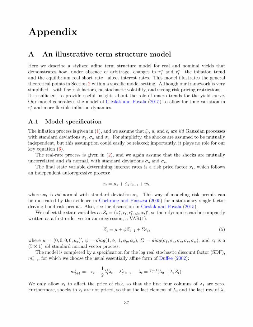
Appendix

A An illustrative term structure model

Here we describe a stylized affine term structure model for real and nominal yields thatdemonstrates how, under absence of arbitrage, changes in π∗t and r∗t—the inflation trendand the equilibrium real short rate—affect interest rates. This model illustrates the generaltheoretical points in Section 2 within a specific model setting. Although our framework is verysimplified—with few risk factors, no stochastic volatility, and strong risk pricing restrictions—it is sufficient to provide useful insights about the role of macro trends for the yield curve.Our model generalizes the model of Cieslak and Povala (2015) to allow for time variation inr∗t and more flexible inflation dynamics.

A.1 Model specification

The inflation process is given in (1), and we assume that ξt, ut and et are iid Gaussian processeswith standard deviations σξ, σu and σe. For simplicity, the shocks are assumed to be mutuallyindependent, but this assumption could easily be relaxed; importantly, it plays no role for ourkey equation (6).

The real-rate process is given in (2), and we again assume that the shocks are mutuallyuncorrelated and iid normal, with standard deviations ση and σv.

The final state variable determining interest rates is a risk price factor xt, which followsan independent autoregressive process:

xt = µx + φxxt−1 + wt,

where wt is iid normal with standard deviation σw. This way of modeling risk premia canbe motivated by the evidence in Cochrane and Piazzesi (2005) for a stationary single factordriving bond risk premia. Also, see the discussion in Cieslak and Povala (2015).

We collect the state variables as Zt = (π∗t , ct, r∗t , gt, xt)

′, so their dynamics can be compactlywritten as a first-order vector autoregression, a VAR(1):

Zt = µ+ φZt−1 + Σεt, (5)

where µ = (0, 0, 0, 0, µx)′, φ = diag(1, φc, 1, φg, φx), Σ = diag(σξ, σu, ση, σv, σw), and εt is a

(5 × 1) iid standard normal vector process.The model is completed by a specification for the log real stochastic discount factor (SDF),

mrt+1, for which we choose the usual essentially affine form of Duffee (2002):

mrt+1 = −rt −

1

2λ′tλt − λ′tεt+1, λt = Σ−1(λ0 + λ1Zt).

We only allow xt to affect the price of risk, so that the first four columns of λ1 are zero.Furthermore, shocks to xt are not priced, so that the last element of λ0 and the last row of λ1

37

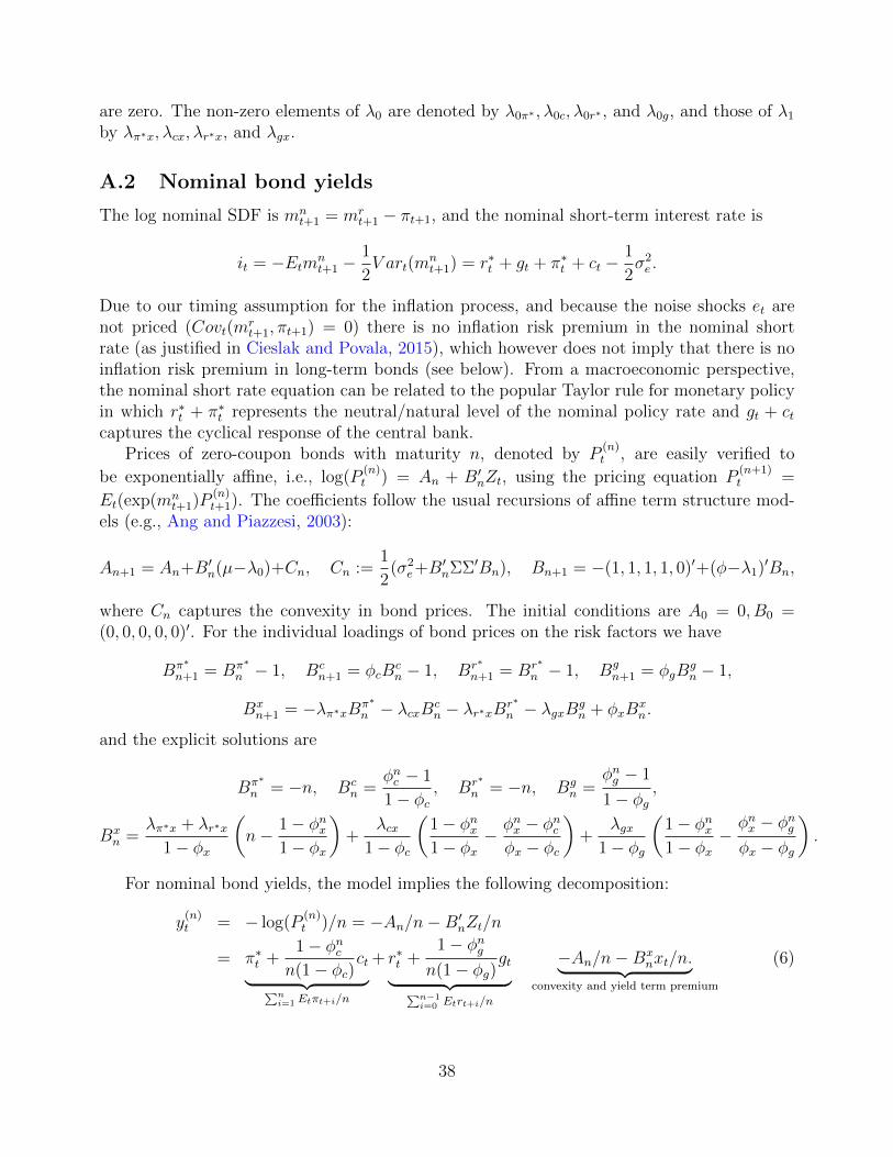
are zero. The non-zero elements of λ0 are denoted by λ0π∗ , λ0c, λ0r∗ , and λ0g, and those of λ1by λπ∗x, λcx, λr∗x, and λgx.

A.2 Nominal bond yields

The log nominal SDF is mnt+1 = mr

t+1 − πt+1, and the nominal short-term interest rate is

it = −Etmnt+1 −

1

2V art(m

nt+1) = r∗t + gt + π∗t + ct −

1

2σ2e .

Due to our timing assumption for the inflation process, and because the noise shocks et arenot priced (Covt(m

rt+1, πt+1) = 0) there is no inflation risk premium in the nominal short

rate (as justified in Cieslak and Povala, 2015), which however does not imply that there is noinflation risk premium in long-term bonds (see below). From a macroeconomic perspective,the nominal short rate equation can be related to the popular Taylor rule for monetary policyin which r∗t + π∗t represents the neutral/natural level of the nominal policy rate and gt + ctcaptures the cyclical response of the central bank.

Prices of zero-coupon bonds with maturity n, denoted by P(n)t , are easily verified to

be exponentially affine, i.e., log(P(n)t ) = An + B′nZt, using the pricing equation P

(n+1)t =

Et(exp(mnt+1)P

(n)t+1). The coefficients follow the usual recursions of affine term structure mod-

els (e.g., Ang and Piazzesi, 2003):

An+1 = An+B′n(µ−λ0)+Cn, Cn :=1

2(σ2

e+B′nΣΣ′Bn), Bn+1 = −(1, 1, 1, 1, 0)′+(φ−λ1)′Bn,

where Cn captures the convexity in bond prices. The initial conditions are A0 = 0, B0 =(0, 0, 0, 0, 0)′. For the individual loadings of bond prices on the risk factors we have

Bπ∗

n+1 = Bπ∗

n − 1, Bcn+1 = φcB

cn − 1, Br∗

n+1 = Br∗

n − 1, Bgn+1 = φgB

gn − 1,

Bxn+1 = −λπ∗xB

π∗

n − λcxBcn − λr∗xB

r∗

n − λgxBgn + φxB

xn.

and the explicit solutions are

Bπ∗

n = −n, Bcn =

φnc − 1

1 − φc, Br∗

n = −n, Bgn =

φng − 1

1 − φg,

Bxn =

λπ∗x + λr∗x1 − φx

(n− 1 − φnx

1 − φx

)+

λcx1 − φc

(1 − φnx1 − φx

− φnx − φncφx − φc

)+

λgx1 − φg

(1 − φnx1 − φx

−φnx − φngφx − φg

).

For nominal bond yields, the model implies the following decomposition:

y(n)t = − log(P

(n)t )/n = −An/n−B′nZt/n

= π∗t +1 − φncn(1 − φc)

ct︸ ︷︷ ︸∑ni=1 Etπt+i/n

+ r∗t +1 − φng

n(1 − φg)gt︸ ︷︷ ︸∑n−1

i=0 Etrt+i/n

−An/n−Bxnxt/n.︸ ︷︷ ︸

convexity and yield term premium

(6)

38

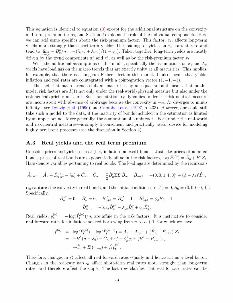
This equation is identical to equation (3) except for the additional structure on the convexityand term premium terms, and Section 2 explains the role of the individual components. Herewe can add some specifics about the risk-premium factor. This factor, xt, affects long-termyields more strongly than short-term yields: The loadings of yields on xt start at zero andtend to lim

n→∞−Bn

x/n = −(λπ∗x + λr∗x)/(1 − φx). Taken together, long-term yields are mostly

driven by the trend components π∗t and r∗t , as well as by the risk-premium factor xt.With the additional assumptions of this model, specifically the assumptions on xt and λt,

yields have loadings on the macro trends that are exactly unity at all maturities. This implies,for example, that there is a long-run Fisher effect in this model. It also means that yields,inflation and real rates are cointegrated with a cointegration vector (1,−1,−1).

The fact that macro trends shift all maturities by an equal amount means that in thismodel risk factors are I(1) not only under the real-world/physical measure but also under therisk-neutral/pricing measure. Such non-stationary dynamics under the risk-neutral measureare inconsistent with absence of arbitrage because the convexity in −An/n diverges to minusinfinity—see Dybvig et al. (1996) and Campbell et al. (1997, p. 433). However, one could stilltake such a model to the data, if the maturity of bonds included in the estimation is limitedby an upper bound. More generally, the assumption of a unit root—both under the real-worldand risk-neutral measures—is simply a convenient and practically useful device for modelinghighly persistent processes (see the discussion in Section 2).

A.3 Real yields and the real term premium

Consider prices and yields of real (i.e., inflation-indexed) bonds. Just like prices of nominal

bonds, prices of real bonds are exponentially affine in the risk factors, log(P(n)t ) = An + B′nZt.

Hats denote variables pertaining to real bonds. The loadings are determined by the recursions

An+1 = An + B′n(µ− λ0) + Cn, Cn :=1

2B′nΣΣ′Bn, Bn+1 = −(0, 0, 1, 1, 0)′ + (φ− λ1)

′Bn,

Cn captures the convexity in real bonds, and the initial conditions are A0 = 0, B0 = (0, 0, 0, 0, 0)′.Specifically,

Bπ∗

n = 0, Bcn = 0, Br∗

n+1 = Br∗

n − 1, Bgn+1 = φgB

gn − 1,

Bxn+1 = −λr∗xBr∗

n − λgxBgn + φxB

xn.

Real yields, y(n)t = − log(P

(n)t )/n, are affine in the risk factors. It is instructive to consider

real forward rates for inflation-indexed borrowing from n to n+ 1, for which we have

f(n)t = log(P

(n)t ) − log(P

(n+1)t ) = An − An+1 + (Bn − Bn+1)

′Zt

= −B′n(µ− λ0) − Cn + r∗t + φnggt + (Bxn − Bx

n+1)xt

= −Cn + Et(rt+n) + ˆftp(n)

t .

Therefore, changes in r∗t affect all real forward rates equally and hence act as a level factor.Changes in the real-rate gap gt affect short-term real rates more strongly than long-termrates, and therefore affect the slope. The last row clarifies that real forward rates can be

39

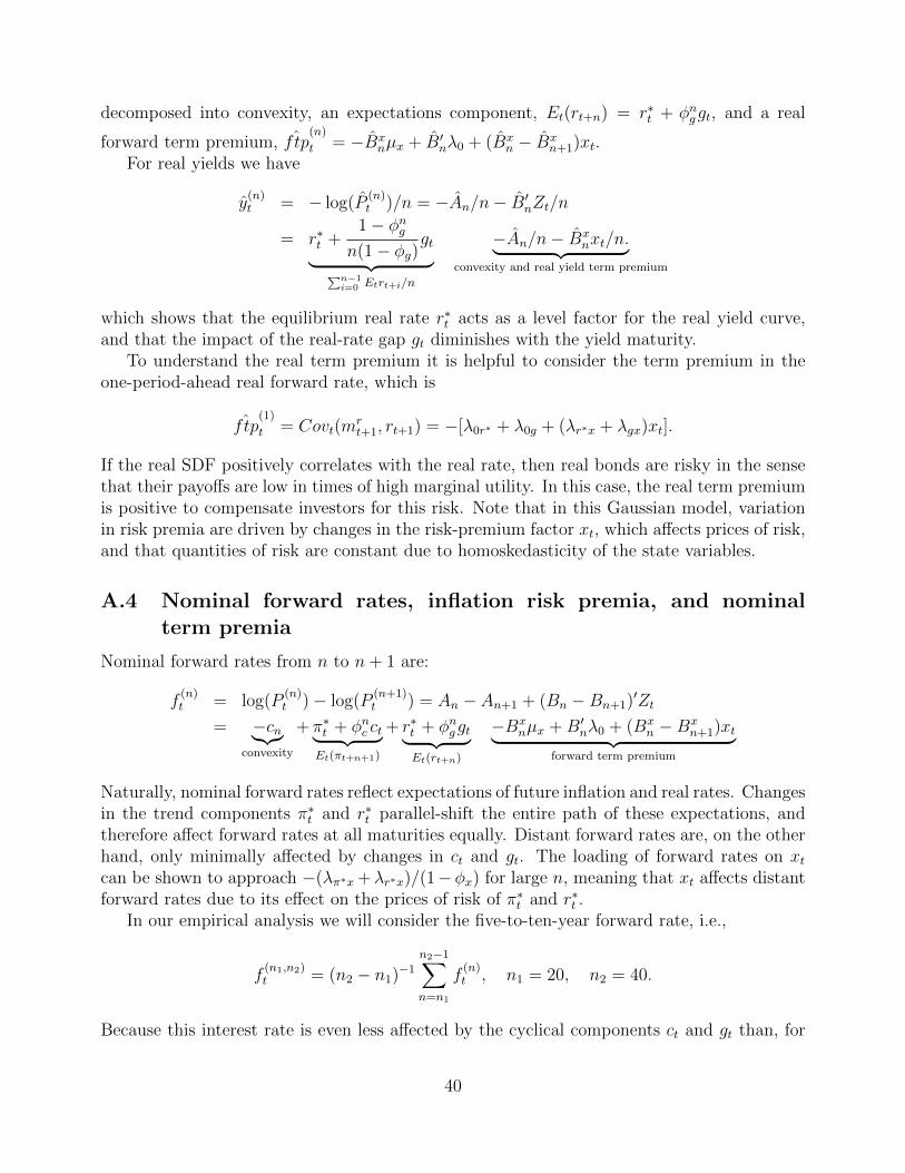
decomposed into convexity, an expectations component, Et(rt+n) = r∗t + φnggt, and a real

forward term premium, ˆftp(n)

t = −Bxnµx + B′nλ0 + (Bx

n − Bxn+1)xt.

For real yields we have

y(n)t = − log(P

(n)t )/n = −An/n− B′nZt/n

= r∗t +1 − φng

n(1 − φg)gt︸ ︷︷ ︸∑n−1

i=0 Etrt+i/n

−An/n− Bxnxt/n.︸ ︷︷ ︸

convexity and real yield term premium

which shows that the equilibrium real rate r∗t acts as a level factor for the real yield curve,and that the impact of the real-rate gap gt diminishes with the yield maturity.

To understand the real term premium it is helpful to consider the term premium in theone-period-ahead real forward rate, which is

ˆftp(1)

t = Covt(mrt+1, rt+1) = −[λ0r∗ + λ0g + (λr∗x + λgx)xt].

If the real SDF positively correlates with the real rate, then real bonds are risky in the sensethat their payoffs are low in times of high marginal utility. In this case, the real term premiumis positive to compensate investors for this risk. Note that in this Gaussian model, variationin risk premia are driven by changes in the risk-premium factor xt, which affects prices of risk,and that quantities of risk are constant due to homoskedasticity of the state variables.

A.4 Nominal forward rates, inflation risk premia, and nominalterm premia

Nominal forward rates from n to n+ 1 are:

f(n)t = log(P

(n)t ) − log(P

(n+1)t ) = An − An+1 + (Bn −Bn+1)

′Zt

= −cn︸︷︷︸convexity

+π∗t + φnc ct︸ ︷︷ ︸Et(πt+n+1)

+ r∗t + φnggt︸ ︷︷ ︸Et(rt+n)

−Bxnµx +B′nλ0 + (Bx

n −Bxn+1)xt︸ ︷︷ ︸

forward term premium

Naturally, nominal forward rates reflect expectations of future inflation and real rates. Changesin the trend components π∗t and r∗t parallel-shift the entire path of these expectations, andtherefore affect forward rates at all maturities equally. Distant forward rates are, on the otherhand, only minimally affected by changes in ct and gt. The loading of forward rates on xtcan be shown to approach −(λπ∗x +λr∗x)/(1−φx) for large n, meaning that xt affects distantforward rates due to its effect on the prices of risk of π∗t and r∗t .

In our empirical analysis we will consider the five-to-ten-year forward rate, i.e.,

f(n1,n2)t = (n2 − n1)

−1n2−1∑n=n1

f(n)t , n1 = 20, n2 = 40.

Because this interest rate is even less affected by the cyclical components ct and gt than, for

40

example, the ten-year yield, it should exhibit a particularly close relationship with the trendcomponents π∗t and r∗t .

The term premium in nominal forward rates, ftp(n)t = −Bx

nµx + B′nλ0 + (Bxn − Bx

n+1)xt,

is composed of the real forward term premium, ˆftp(n)

t , and a forward inflation risk premium,

firp(n)t . The intuition is again easiest for n = 1:

firp(1)t = Covt(m

rt+1, Et+1(πt+2)) = −[λ0π∗ + λ0c + (λπ∗x + λcx)xt].

If shocks to inflation expectations are positively correlated with the real SDF, then nominalbonds are more risky than real bonds and require a higher risk premium, i.e., a positiveinflation risk premium. Like the real term premium, the inflation risk premium in this modelis driven only by changes in xt.

A.5 Excess bond returns

In this illustrative model, as in Cieslak and Povala (2015)’s model, excess bond returns, rx(n)t+1,

are driven only by the risk premium factor xt:

rx(n)t+1 = p

(n−1)t+1 − p

(n)t − y

(1)t = −1

2B′n−1ΣΣ′Bn−1 +B′n−1(λ0 + λ1ι5)xt +B′n−1Σεt+1,

where p(n)t denotes the log-price of a zero-coupon bond with maturity of n quarters and ι5 is

a (5 × 1)-vector of ones.

A.6 Variance ratios

The model implies analytical expressions for the variance ratios in Section 8. For one-periodand h-period innovations, respectively, they are

V R(n)1 =

σ2ξ + ac(n)σ2

u

σ2ξ + ac(n)σ2

u + σ2η + ag(n)σ2

v +(Bxnn

)2σ2w

,

V R(n)h =

hσ2ξ + ac(n)bc(h)σ2

u

hσ2ξ + ac(n)bc(h)σ2

u + hσ2η + ag(n)bg(h)σ2

v +(Bxnn

)2bx(h)σ2

w

,

ai(n) =

(1 − φnin(1 − φi)

)2

, bi(h) =1 − φ2h

i

1 − φ2i

, i = c, g, x.

These expressions can help elucidate the factors determining the variance ratios. Note thatfor arbitrarily long maturity

limn→∞

V R(n)1 =

σ2ξ

σ2ξ + σ2

η +(λπ∗x+λr∗x

1−φx

)2σ2w

.

41

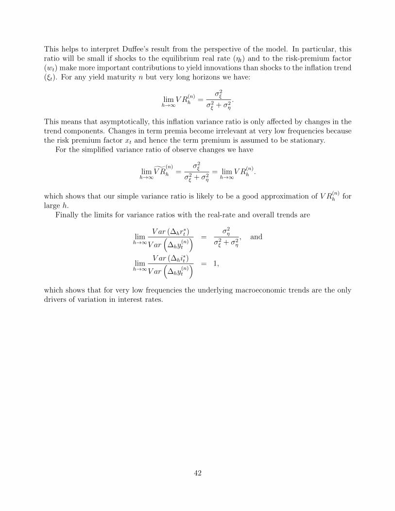
This helps to interpret Duffee’s result from the perspective of the model. In particular, thisratio will be small if shocks to the equilibrium real rate (ηt) and to the risk-premium factor(wt) make more important contributions to yield innovations than shocks to the inflation trend(ξt). For any yield maturity n but very long horizons we have:

limh→∞

V R(n)h =

σ2ξ

σ2ξ + σ2

η

.

This means that asymptotically, this inflation variance ratio is only affected by changes in thetrend components. Changes in term premia become irrelevant at very low frequencies becausethe risk premium factor xt and hence the term premium is assumed to be stationary.

For the simplified variance ratio of observe changes we have

limh→∞

V R(n)

h =σ2ξ

σ2ξ + σ2

η

= limh→∞

V R(n)h .

which shows that our simple variance ratio is likely to be a good approximation of V R(n)h for

large h.Finally the limits for variance ratios with the real-rate and overall trends are

limh→∞

V ar (∆hr∗t )

V ar(

∆hy(n)t

) =σ2η

σ2ξ + σ2

η

, and

limh→∞

V ar (∆hi∗t )

V ar(

∆hy(n)t

) = 1,

which shows that for very low frequencies the underlying macroeconomic trends are the onlydrivers of variation in interest rates.

42

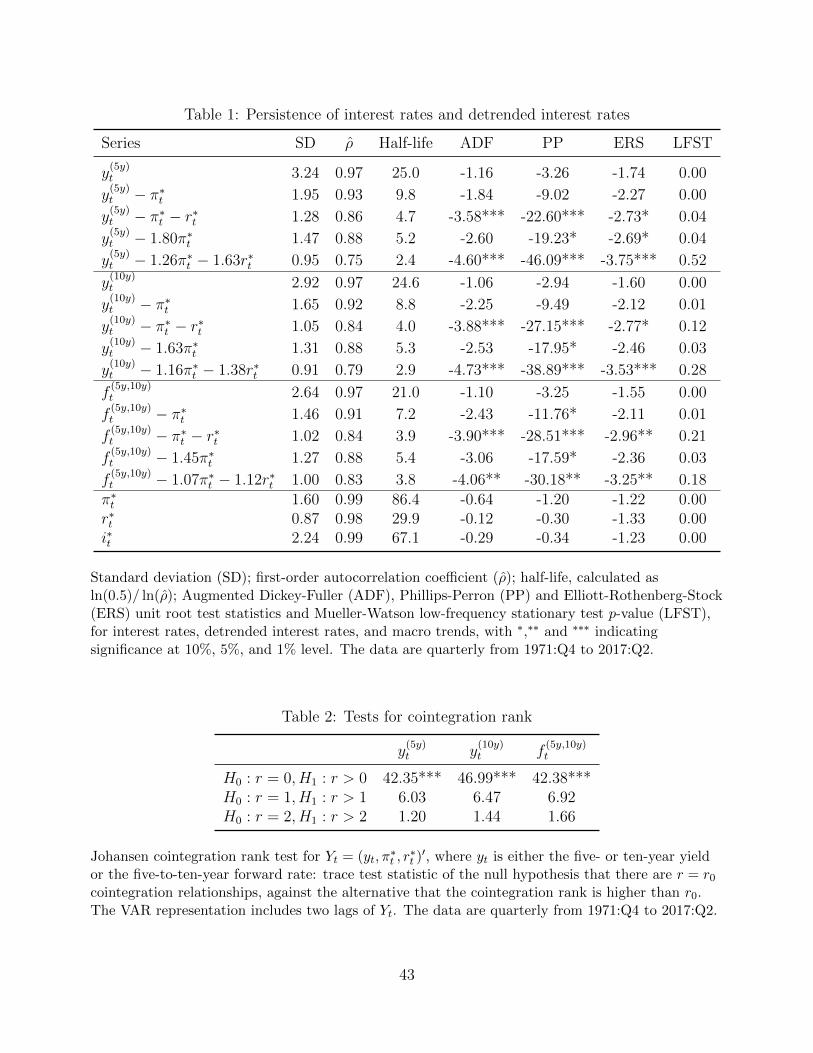
Table 1: Persistence of interest rates and detrended interest rates

Series SD ρ Half-life ADF PP ERS LFST

y(5y)t 3.24 0.97 25.0 -1.16 -3.26 -1.74 0.00

y(5y)t − π∗t 1.95 0.93 9.8 -1.84 -9.02 -2.27 0.00

y(5y)t − π∗t − r∗t 1.28 0.86 4.7 -3.58*** -22.60*** -2.73* 0.04

y(5y)t − 1.80π∗t 1.47 0.88 5.2 -2.60 -19.23* -2.69* 0.04

y(5y)t − 1.26π∗t − 1.63r∗t 0.95 0.75 2.4 -4.60*** -46.09*** -3.75*** 0.52

y(10y)t 2.92 0.97 24.6 -1.06 -2.94 -1.60 0.00

y(10y)t − π∗t 1.65 0.92 8.8 -2.25 -9.49 -2.12 0.01

y(10y)t − π∗t − r∗t 1.05 0.84 4.0 -3.88*** -27.15*** -2.77* 0.12

y(10y)t − 1.63π∗t 1.31 0.88 5.3 -2.53 -17.95* -2.46 0.03

y(10y)t − 1.16π∗t − 1.38r∗t 0.91 0.79 2.9 -4.73*** -38.89*** -3.53*** 0.28

f(5y,10y)t 2.64 0.97 21.0 -1.10 -3.25 -1.55 0.00

f(5y,10y)t − π∗t 1.46 0.91 7.2 -2.43 -11.76* -2.11 0.01

f(5y,10y)t − π∗t − r∗t 1.02 0.84 3.9 -3.90*** -28.51*** -2.96** 0.21

f(5y,10y)t − 1.45π∗t 1.27 0.88 5.4 -3.06 -17.59* -2.36 0.03

f(5y,10y)t − 1.07π∗t − 1.12r∗t 1.00 0.83 3.8 -4.06** -30.18** -3.25** 0.18π∗t 1.60 0.99 86.4 -0.64 -1.20 -1.22 0.00r∗t 0.87 0.98 29.9 -0.12 -0.30 -1.33 0.00i∗t 2.24 0.99 67.1 -0.29 -0.34 -1.23 0.00

Standard deviation (SD); first-order autocorrelation coefficient (ρ); half-life, calculated asln(0.5)/ ln(ρ); Augmented Dickey-Fuller (ADF), Phillips-Perron (PP) and Elliott-Rothenberg-Stock(ERS) unit root test statistics and Mueller-Watson low-frequency stationary test p-value (LFST),for interest rates, detrended interest rates, and macro trends, with ∗,∗∗ and ∗∗∗ indicatingsignificance at 10%, 5%, and 1% level. The data are quarterly from 1971:Q4 to 2017:Q2.

Table 2: Tests for cointegration rank

y(5y)t y

(10y)t f

(5y,10y)t

H0 : r = 0, H1 : r > 0 42.35*** 46.99*** 42.38***H0 : r = 1, H1 : r > 1 6.03 6.47 6.92H0 : r = 2, H1 : r > 2 1.20 1.44 1.66

Johansen cointegration rank test for Yt = (yt, π∗t , r∗t )′, where yt is either the five- or ten-year yield

or the five-to-ten-year forward rate: trace test statistic of the null hypothesis that there are r = r0cointegration relationships, against the alternative that the cointegration rank is higher than r0.The VAR representation includes two lags of Yt. The data are quarterly from 1971:Q4 to 2017:Q2.

43

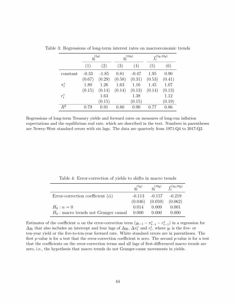
Table 3: Regressions of long-term interest rates on macroeconomic trends

y(5y)t y

(10y)t f

(5y,10y)t

(1) (2) (3) (4) (5) (6)

constant -0.33 -1.85 0.81 -0.47 1.95 0.90(0.67) (0.29) (0.58) (0.31) (0.53) (0.41)

π∗t 1.80 1.26 1.63 1.16 1.45 1.07(0.15) (0.14) (0.14) (0.13) (0.14) (0.13)

r∗t 1.63 1.38 1.12(0.15) (0.15) (0.19)

R2 0.79 0.91 0.80 0.90 0.77 0.86

Regressions of long-term Treasury yields and forward rates on measures of long-run inflationexpectations and the equilibrium real rate, which are described in the text. Numbers in parenthesesare Newey-West standard errors with six lags. The data are quarterly from 1971:Q4 to 2017:Q2.

Table 4: Error-correction of yields to shifts in macro trends

y(5y)t y

(10y)t f

(5y,10y)t

Error-correction coefficient (α) -0.113 -0.157 -0.219(0.046) (0.059) (0.062)

H0 : α = 0 0.014 0.009 0.001H0 : macro trends not Granger causal 0.000 0.000 0.000

Estimates of the coefficient α on the error-correction term (yt−1 − π∗t−1 − r∗t−1) in a regression for∆yt that also includes an intercept and four lags of ∆yt, ∆π∗t and r∗t , where yt is the five- orten-year yield or the five-to-ten-year forward rate. White standard errors are in parentheses. Thefirst p-value is for a test that the error-correction coefficient is zero. The second p-value is for a testthat the coefficients on the error-correction terms and all lags of first-differenced macro trends arezero, i.e., the hypothesis that macro trends do not Granger-cause movements in yields.

44

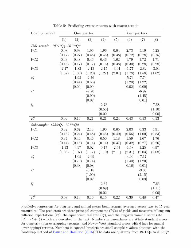
Table 5: Predicting excess returns with macro trends

Holding period: One quarter Four quarters

(1) (2) (3) (4) (5) (6) (7) (8)

Full sample: 1971:Q4–2017:Q2PC1 0.08 0.98 1.96 1.96 0.04 2.73 5.19 5.25

(0.17) (0.27) (0.48) (0.45) (0.38) (0.72) (0.78) (0.75)PC2 0.43 0.48 0.46 0.46 1.62 1.79 1.72 1.71

(0.18) (0.17) (0.17) (0.16) (0.38) (0.30) (0.28) (0.28)PC3 -2.47 -1.82 -2.13 -2.15 -3.91 -1.77 -2.82 -3.04

(1.37) (1.30) (1.20) (1.27) (2.07) (1.78) (1.58) (1.62)π∗t -1.95 -2.76 -5.74 -7.74

(0.44) (0.53) (1.20) (1.22)[0.00] [0.00] [0.02] [0.00]

r∗t -2.70 -6.97(0.90) (1.45)[0.02] [0.01]

i∗t -2.75 -7.58(0.55) (1.10)[0.00] [0.00]

R2 0.09 0.16 0.21 0.21 0.24 0.43 0.53 0.53

Subsample: 1985:Q1–2017:Q2PC1 0.32 0.67 2.13 1.90 0.65 2.03 6.33 5.91

(0.16) (0.24) (0.48) (0.45) (0.40) (0.56) (1.00) (0.83)PC2 0.34 0.44 0.46 0.50 1.18 1.59 1.67 1.76

(0.14) (0.15) (0.14) (0.14) (0.37) (0.32) (0.27) (0.26)PC3 -1.13 -0.97 0.02 -0.17 -2.67 -1.68 1.25 0.97

(1.08) (1.07) (1.17) (1.10) (2.11) (2.31) (2.03) (2.08)π∗t -1.05 -2.09 -4.06 -7.17

(0.73) (0.74) (1.40) (1.20)[0.38] [0.08] [0.16] [0.01]

r∗t -3.18 -9.38(1.00) (2.15)[0.02] [0.03]

i∗t -2.32 -7.66(0.69) (1.11)[0.02] [0.00]

R2 0.08 0.10 0.16 0.15 0.22 0.30 0.48 0.47

Predictive regressions for quarterly and annual excess bond returns, averaged across two- to 15-yearmaturities. The predictors are three principal components (PCs) of yields and measures of long-runinflation expectations (π∗t ), the equilibrium real rate (r∗t ), and the long-run nominal short rate(i∗t = π∗t + r∗t ) which are described in the text. Numbers in parentheses are White standard errorsfor quarterly (non-overlapping) returns, and Newey-West standard errors with 6 lags for annual(overlapping) returns. Numbers in squared brackets are small-sample p-values obtained with thebootstrap method of Bauer and Hamilton (2016). The data are quarterly from 1971:Q4 to 2017:Q2.

45

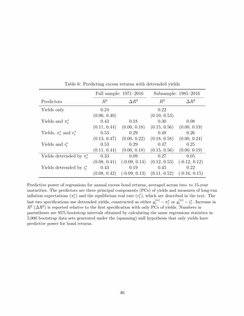
Table 6: Predicting excess returns with detrended yields

Full sample: 1971–2016 Subsample: 1985–2016

Predictors R2 ∆R2 R2 ∆R2

Yields only 0.24 0.22(0.06, 0.40) (0.10, 0.53)

Yields and π∗t 0.43 0.18 0.30 0.08(0.11, 0.44) (0.00, 0.18) (0.15, 0.56) (0.00, 0.19)

Yields, π∗t and r∗t 0.53 0.29 0.48 0.26(0.13, 0.47) (0.00, 0.22) (0.18, 0.58) (0.00, 0.24)

Yields and i∗t 0.53 0.29 0.47 0.25(0.11, 0.44) (0.00, 0.18) (0.15, 0.56) (0.00, 0.19)

Yields detrended by π∗t 0.33 0.09 0.27 0.05(0.08, 0.41) (-0.09, 0.14) (0.12, 0.53) (-0.12, 0.12)

Yields detrended by i∗t 0.43 0.19 0.45 0.22(0.08, 0.42) (-0.09, 0.13) (0.11, 0.52) (-0.16, 0.15)

Predictive power of regressions for annual excess bond returns, averaged across two- to 15-yearmaturities. The predictors are three principal components (PCs) of yields and measures of long-runinflation expectations (π∗t ) and the equilibrium real rate (r∗t ), which are described in the text. The

last two specifications use detrended yields, constructed as either y(n)t − π∗t or y

(n)t − i∗t . Increase in

R2 (∆R2) is reported relative to the first specification with only PCs of yields. Numbers inparentheses are 95%-bootstrap intervals obtained by calculating the same regressions statistics in5,000 bootstrap data sets generated under the (spanning) null hypothesis that only yields havepredictive power for bond returns.

46

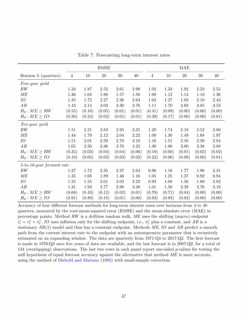
Table 7: Forecasting long-term interest rates

RMSE MAE

Horizon h (quarters): 4 10 20 30 40 4 10 20 30 40

Five-year yieldRW 1.34 1.87 2.52 2.61 2.90 1.02 1.33 1.92 2.23 2.55ME 1.36 1.64 1.86 1.57 1.56 1.00 1.12 1.14 1.10 1.36IO 1.35 1.72 2.27 2.36 2.63 1.02 1.27 1.83 2.10 2.43AR 1.43 2.14 3.03 3.30 3.76 1.11 1.70 2.68 3.05 3.53H0 : ME ≥ RW (0.55) (0.16) (0.05) (0.01) (0.01) (0.41) (0.09) (0.00) (0.00) (0.00)H0 : ME ≥ IO (0.56) (0.24) (0.02) (0.01) (0.01) (0.39) (0.17) (0.00) (0.00) (0.01)

Ten-year yieldRW 1.51 2.21 2.83 2.95 3.25 1.20 1.74 2.18 2.52 2.80ME 1.44 1.79 2.12 2.04 2.22 1.09 1.30 1.49 1.68 1.97IO 1.51 2.01 2.59 2.78 3.10 1.16 1.51 2.16 2.50 2.84AR 1.65 2.50 3.36 3.70 4.22 1.30 1.98 3.00 3.38 3.88H0 : ME ≥ RW (0.35) (0.03) (0.04) (0.04) (0.06) (0.19) (0.00) (0.01) (0.02) (0.02)H0 : ME ≥ IO (0.19) (0.05) (0.02) (0.02) (0.02) (0.22) (0.06) (0.00) (0.00) (0.01)

5-to-10-year forward rateRW 1.27 1.72 2.35 2.37 2.64 0.96 1.16 1.77 1.96 2.31ME 1.35 1.68 1.89 1.46 1.16 1.05 1.25 1.27 0.92 0.94IO 1.25 1.55 2.01 2.02 2.22 0.93 1.08 1.50 1.69 2.02AR 1.31 1.93 2.77 2.98 3.38 1.01 1.50 2.39 2.76 3.19H0 : ME ≥ RW (0.68) (0.43) (0.12) (0.02) (0.01) (0.79) (0.71) (0.04) (0.00) (0.00)H0 : ME ≥ IO (0.91) (0.89) (0.18) (0.01) (0.00) (0.93) (0.93) (0.02) (0.00) (0.00)

Accuracy of four different forecast methods for long-term interest rates over horizons from 4 to 40quarters, measured by the root-mean-squared error (RMSE) and the mean-absolute error (MAE) inpercentage points. Method RW is a driftless random walk, ME uses the shifting (macro) endpointi∗t = r∗t + π∗t , IO uses inflation only for the shifting endpoint, i.e., π∗t plus a constant, and AR is astationary AR(1) model and thus has a constant endpoint. Methods ME, IO and AR predict a smoothpath from the current interest rate to the endpoint with an autoregressive parameter that is recursivelyestimated on an expanding window. The data are quarterly from 1971:Q4 to 2017:Q2. The first forecastis made in 1976:Q3 once five years of data are available, and the last forecast is in 2007:Q2, for a total of124 (overlapping) observations. The last two rows in each panel report one-sided p-values for testing thenull hypothesis of equal forecast accuracy against the alternative that method ME is more accurate,using the method of Diebold and Mariano (1995) with small-sample correction.

47

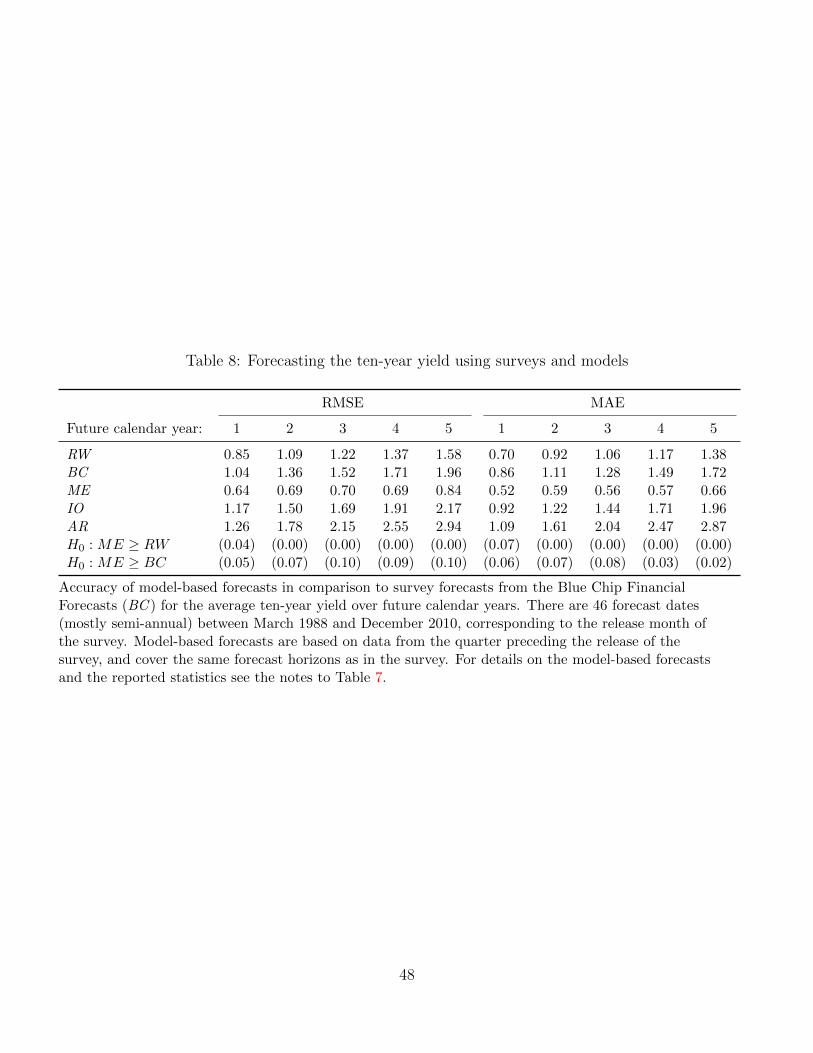
Table 8: Forecasting the ten-year yield using surveys and models

RMSE MAE

Future calendar year: 1 2 3 4 5 1 2 3 4 5

RW 0.85 1.09 1.22 1.37 1.58 0.70 0.92 1.06 1.17 1.38BC 1.04 1.36 1.52 1.71 1.96 0.86 1.11 1.28 1.49 1.72ME 0.64 0.69 0.70 0.69 0.84 0.52 0.59 0.56 0.57 0.66IO 1.17 1.50 1.69 1.91 2.17 0.92 1.22 1.44 1.71 1.96AR 1.26 1.78 2.15 2.55 2.94 1.09 1.61 2.04 2.47 2.87H0 : ME ≥ RW (0.04) (0.00) (0.00) (0.00) (0.00) (0.07) (0.00) (0.00) (0.00) (0.00)H0 : ME ≥ BC (0.05) (0.07) (0.10) (0.09) (0.10) (0.06) (0.07) (0.08) (0.03) (0.02)

Accuracy of model-based forecasts in comparison to survey forecasts from the Blue Chip FinancialForecasts (BC ) for the average ten-year yield over future calendar years. There are 46 forecast dates(mostly semi-annual) between March 1988 and December 2010, corresponding to the release month ofthe survey. Model-based forecasts are based on data from the quarter preceding the release of thesurvey, and cover the same forecast horizons as in the survey. For details on the model-based forecastsand the reported statistics see the notes to Table 7.

48

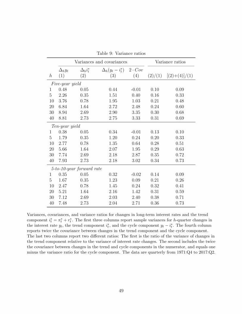
Table 9: Variance ratios

Variances and covariances Variance ratios

∆hyt ∆hi∗t ∆h(yt − i∗t ) 2 · Cov

h (1) (2) (3) (4) (2)/(1) [(2)+(4)]/(1)

Five-year yield1 0.48 0.05 0.44 -0.01 0.10 0.095 2.26 0.35 1.51 0.40 0.16 0.3310 3.76 0.78 1.95 1.03 0.21 0.4820 6.84 1.64 2.72 2.48 0.24 0.6030 8.94 2.69 2.90 3.35 0.30 0.6840 8.81 2.73 2.75 3.33 0.31 0.69

Ten-year yield1 0.38 0.05 0.34 -0.01 0.13 0.105 1.79 0.35 1.20 0.24 0.20 0.3310 2.77 0.78 1.35 0.64 0.28 0.5120 5.66 1.64 2.07 1.95 0.29 0.6330 7.74 2.69 2.18 2.87 0.35 0.7240 7.93 2.73 2.18 3.02 0.34 0.73

5-to-10-year forward rate1 0.35 0.05 0.32 -0.02 0.14 0.095 1.67 0.35 1.23 0.09 0.21 0.2610 2.47 0.78 1.45 0.24 0.32 0.4120 5.21 1.64 2.16 1.42 0.31 0.5930 7.12 2.69 2.03 2.40 0.38 0.7140 7.48 2.73 2.04 2.71 0.36 0.73

Variances, covariances, and variance ratios for changes in long-term interest rates and the trendcomponent i∗t = π∗t + r∗t . The first three columns report sample variances for h-quarter changes inthe interest rate yt, the trend component i∗t , and the cycle component yt − i∗t . The fourth columnreports twice the covariance between changes in the trend component and the cycle component.The last two columns report two different ratios: The first is the ratio of the variance of changes inthe trend component relative to the variance of interest rate changes. The second includes the twicethe covariance between changes in the trend and cycle components in the numerator, and equals oneminus the variance ratio for the cycle component. The data are quarterly from 1971:Q4 to 2017:Q2.

49

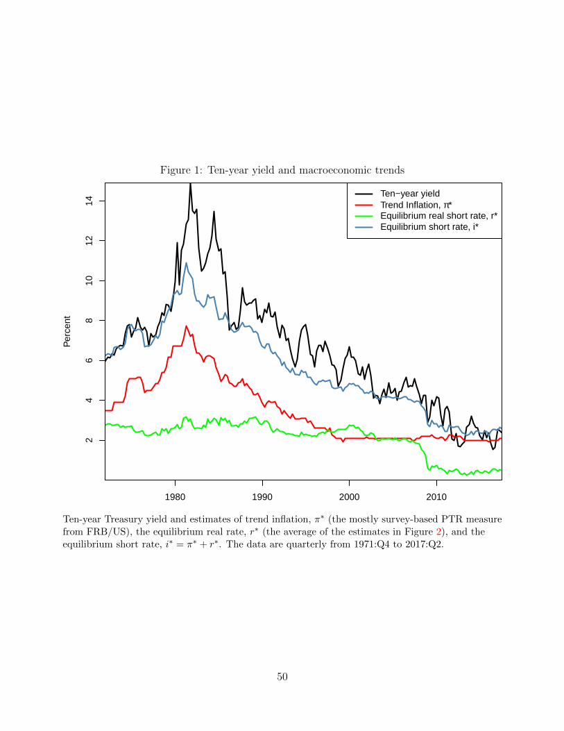
Figure 1: Ten-year yield and macroeconomic trends

1980 1990 2000 2010

24

68

1012

14

Per

cent

Ten−year yieldTrend Inflation, π*Equilibrium real short rate, r*Equilibrium short rate, i*

Ten-year Treasury yield and estimates of trend inflation, π∗ (the mostly survey-based PTR measurefrom FRB/US), the equilibrium real rate, r∗ (the average of the estimates in Figure 2), and theequilibrium short rate, i∗ = π∗ + r∗. The data are quarterly from 1971:Q4 to 2017:Q2.

50

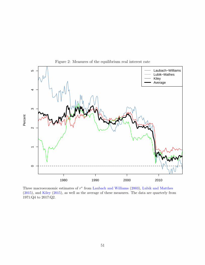
Figure 2: Measures of the equilibrium real interest rate

1980 1990 2000 2010

01

23

45

Per

cent

Laubach−WilliamsLubik−MathesKileyAverage

Three macroeconomic estimates of r∗ from Laubach and Williams (2003), Lubik and Matthes(2015), and Kiley (2015), as well as the average of these measures. The data are quarterly from1971:Q4 to 2017:Q2.

51

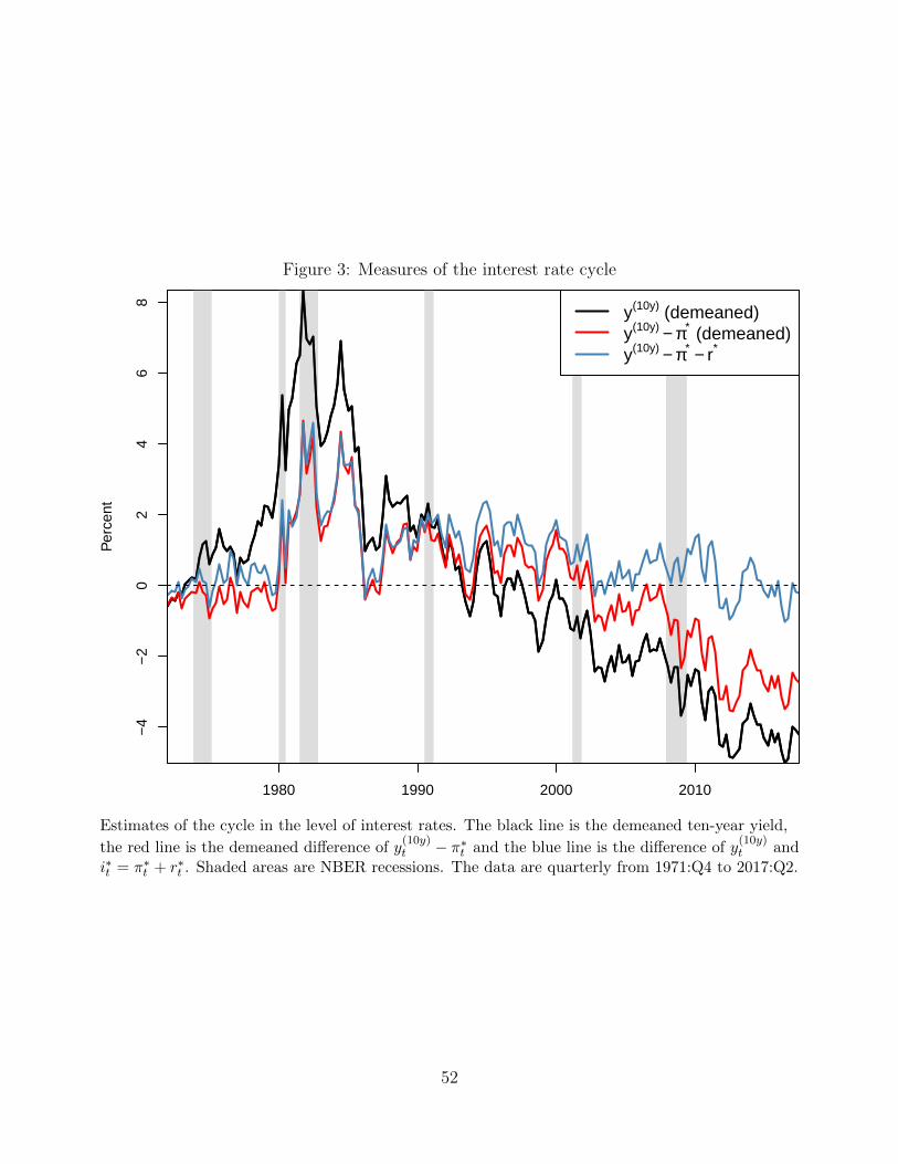
Figure 3: Measures of the interest rate cycle

1980 1990 2000 2010

−4

−2

02

46

8

Per

cent

y(10y) (demeaned)y(10y) − π∗ (demeaned)y(10y) − π∗ − r∗

Estimates of the cycle in the level of interest rates. The black line is the demeaned ten-year yield,

the red line is the demeaned difference of y(10y)t − π∗t and the blue line is the difference of y

(10y)t and

i∗t = π∗t + r∗t . Shaded areas are NBER recessions. The data are quarterly from 1971:Q4 to 2017:Q2.

52

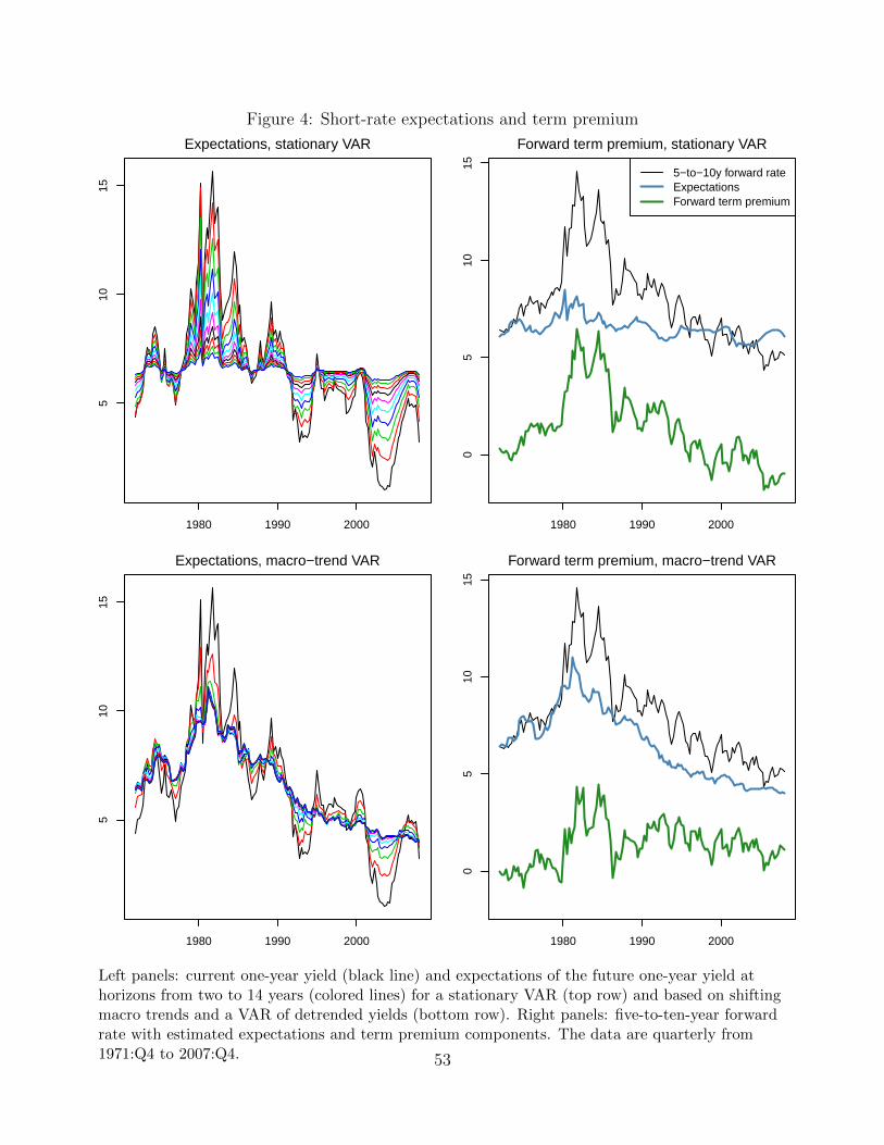
Figure 4: Short-rate expectations and term premium5

1015

Expectations, stationary VAR

Per

cent

1980 1990 2000

510

15

Expectations, macro−trend VAR

Per

cent

1980 1990 2000

1980 1990 2000

05

1015

Forward term premium, stationary VAR

Per

cent

5−to−10y forward rateExpectationsForward term premium

1980 1990 2000

05

1015

Forward term premium, macro−trend VAR

Per

cent

Left panels: current one-year yield (black line) and expectations of the future one-year yield athorizons from two to 14 years (colored lines) for a stationary VAR (top row) and based on shiftingmacro trends and a VAR of detrended yields (bottom row). Right panels: five-to-ten-year forwardrate with estimated expectations and term premium components. The data are quarterly from1971:Q4 to 2007:Q4. 53

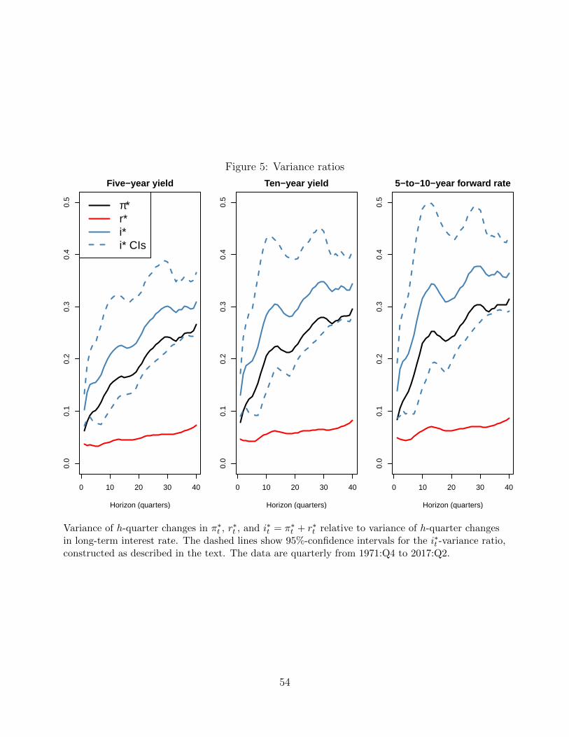
Figure 5: Variance ratios

0 10 20 30 40

0.0

0.1

0.2

0.3

0.4

0.5

Five−year yield

Horizon (quarters)

π*r*i*i* CIs

0 10 20 30 40

0.0

0.1

0.2

0.3

0.4

0.5

Ten−year yield

Horizon (quarters)

0 10 20 30 40

0.0

0.1

0.2

0.3

0.4

0.5

5−to−10−year forward rate

Horizon (quarters)

Variance of h-quarter changes in π∗t , r∗t , and i∗t = π∗t + r∗t relative to variance of h-quarter changes

in long-term interest rate. The dashed lines show 95%-confidence intervals for the i∗t -variance ratio,constructed as described in the text. The data are quarterly from 1971:Q4 to 2017:Q2.

54