Integral Geometry & Geometric Probabilitytreiberg/IntGeomSlides.pdf · Luis A. Santal´o, Integral Geometry and Geometric Probability, Addison-Wesley, Reading, MA, 1976. ... Figure:

University of Utah Undergraduate Colloquium

Integral Geometry & Geometric Probability

Andrejs Treibergs

University of Utah

Wednesday, October 1, 2008

2. References

Presented to the Undergraduate Colloquium, University of Utah,Salt lake City, Utah on October 7, 2008.

This talk has also been presented to the 2008 Summer MathematicsResearch Experience for Undergraduates (REU) Seminar at BrighamYoung University, Provo, Utah on July 29, 2008.

URL of Beamer Slides: “Integral Geometry and Geometric Probability”

http://www.math.utah.edu/treiberg/IntGeomSlides.pdf

Some excellent references to Integral Geometry.

Luis A. Santalo, Integral Geometry and Geometric Probability,Addison-Wesley, Reading, MA, 1976.

Herbert Solomon, Geometric Probability (CBMS-NSF RegionalConference Series in Applied Mathematics 28), Society for Industrialand Applied Mathetaics, Philadelphia, 1978.

Wilhelm Blaschke, Vorlesungen uber Integralgeometrie I, II, Chelsea,New York, 1949, (2nd ed. orig. pub. B. G. Teubner, Leipzig, 1935.)

3. Outline.

Integral Geometry, known in applied circles as Geometric Probability, issomewhat of a mathematical antique (and therefore it is a favorite ofmine!) From it developed many modern topics: geometric measuretheory, stereometry, tomography, characteristic classes. . .

1 Integral geometry examples:

Buffon’s needle problem.Firery’s dice problem

2 Kinematic measure.

3 Poincare’s Formula for average number of intersections of curves.

4 Cauchy’s Formula for the average projected length.

5 Crofton’s Formula for the average chord length.

6 Santalo’s & Blaschke’s Formuls for the averages over the of theintesection of two domains.

7 Application to the Isoperimetric Inequality.

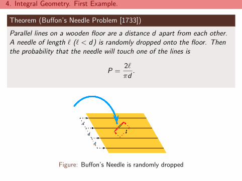
4. Integral Geometry. First Example.

Theorem (Buffon’s Needle Problem [1733])

Parallel lines on a wooden floor are a distance d apart from each other.A needle of length ` (` < d) is randomly dropped onto the floor. Thenthe probability that the needle will touch one of the lines is

P =2`

πd.

Figure: Buffon’s Needle is randomly dropped

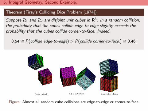
5. Integral Geometry. Second Example.

Theorem (Firey’s Colliding Dice Problem [1974])

Suppose Ω1 and Ω2 are disjoint unit cubes in R3. In a random collision,the probablity that the cubes collide edge-to-edge slightly exceeds theprobability that the cubes collide corner-to-face. Indeed,

0.54 ∼= P(collide edge-to-edge) > P(collide corner-to-face.) ∼= 0.46.

Figure: Almost all random cube collisions are edge-to-edge or corner-to-face.

6. Coordinates of a line.

An unoriented line in the plane is determined by two numbers, p thedistance to the origin and θ, the direction to the closest point.The variable range is 0 ≤ p and 0 ≤ θ < 2π.Equivalently, we may take the range −∞ < p <∞ and 0 ≤ η < π.

Figure: (p, θ) coordinates for the line L.

The equation of the line L(p, θ) in Cartesian coordinates is

cos(θ)x + sin(θ)y = p (1)

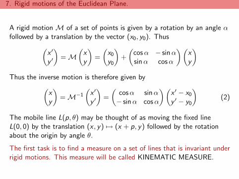
7. Rigid motions of the Euclidean Plane.

A rigid motion M of a set of points is given by a rotation by an angle αfollowed by a translation by the vector (x0, y0). Thus(

x ′

y ′

)= M

(xy

)=

(x0

y0

)+

(cosα − sinαsinα cosα

)(xy

)Thus the inverse motion is therefore given by(

xy

)= M−1

(x ′

y ′

)=

(cosα sinα− sinα cosα

)(x ′ − x0

y ′ − y0

)(2)

The mobile line L(p, θ) may be thought of as moving the fixed lineL(0, 0) by the translation (x , y) 7→ (x + p, y) followed by the rotationabout the origin by angle θ.

The first task is to find a measure on a set of lines that is invariant underrigid motions. This measure will be called KINEMATIC MEASURE.

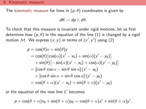
8. Kinematic measure.

The kinematic measure for lines in (p, θ) coordinates is given by

dK = dp ∧ dθ.

To check that this measure is invariant under rigid motions, let us firstdetermine how (p, θ) in the equation of the line (1) is changed by a rigidmotion M. We express (x , y) in terms of (x ′, y ′) using (2)

p = cos(θ)x + sin(θ)y

= cos(θ)[cos(α)(x ′ − x0) + sin(α)(y ′ − y0)

]+ sin(θ)

[− sin(α)(x ′ − x0) + cos(α)(y ′ − y0)

]= [cos θ cosα− sin θ sinα] (x ′ − x0)

+ [cos θ sinα+ sin θ cosα] (y ′ − y0)

= cos(θ + α)(x ′ − x0) + sin(θ + α)(y ′ − y0)

or the equation of the new line L′ becomes

p + cos(θ + α)x0 + sin(θ + α)y0 = cos(θ + α)x ′ + sin(θ + α)y ′.

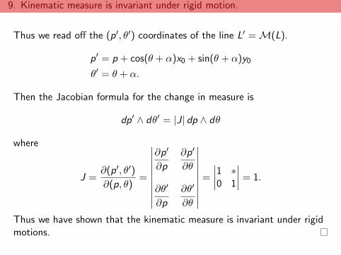
9. Kinematic measure is invariant under rigid motion.

Thus we read off the (p′, θ′) coordinates of the line L′ = M(L).

p′ = p + cos(θ + α)x0 + sin(θ + α)y0

θ′ = θ + α.

Then the Jacobian formula for the change in measure is

dp′ ∧ dθ′ = |J| dp ∧ dθ

where

J =∂(p′, θ′)

∂(p, θ)=

∣∣∣∣∣∣∣∣∣∣∂p′

∂p

∂p′

∂θ

∂θ′

∂p

∂θ′

∂θ

∣∣∣∣∣∣∣∣∣∣=

∣∣∣∣1 ∗0 1

∣∣∣∣ = 1.

Thus we have shown that the kinematic measure is invariant under rigidmotions.

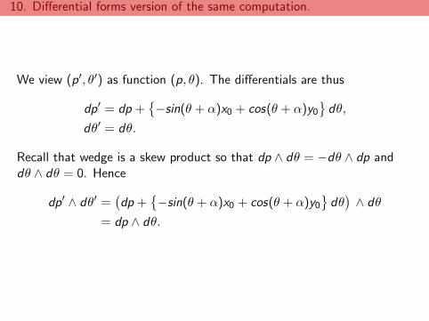
10. Differential forms version of the same computation.

We view (p′, θ′) as function (p, θ). The differentials are thus

dp′ = dp +−sin(θ + α)x0 + cos(θ + α)y0

dθ,

dθ′ = dθ.

Recall that wedge is a skew product so that dp ∧ dθ = −dθ ∧ dp anddθ ∧ dθ = 0. Hence

dp′ ∧ dθ′ =(dp +

−sin(θ + α)x0 + cos(θ + α)y0

dθ)∧ dθ

= dp ∧ dθ.

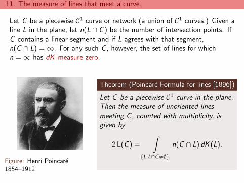
11. The measure of lines that meet a curve.

Let C be a piecewise C1 curve or network (a union of C1 curves.) Given aline L in the plane, let n(L ∩ C ) be the number of intersection points. IfC contains a linear segment and if L agrees with that segment,n(C ∩ L) = ∞. For any such C , however, the set of lines for whichn = ∞ has dK -measure zero.

Figure: Henri Poincare1854–1912

Theorem (Poincare Formula for lines [1896])

Let C be a piecewise C1 curve in the plane.Then the measure of unoriented linesmeeting C, counted with multiplicity, isgiven by

2 L(C ) =

∫L:L∩C 6=∅

n(C ∩ L) dK (L).

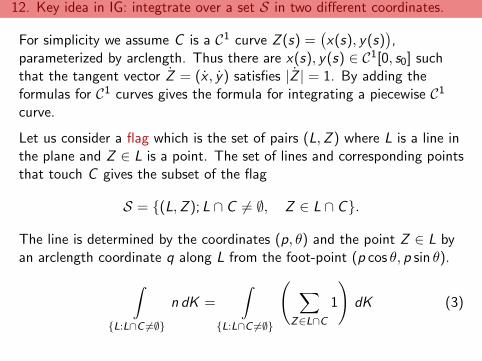
12. Key idea in IG: integtrate over a set S in two different coordinates.

For simplicity we assume C is a C1 curve Z (s) =(x(s), y(s)

),

parameterized by arclength. Thus there are x(s), y(s) ∈ C1[0, s0] suchthat the tangent vector Z = (x , y) satisfies |Z | = 1. By adding theformulas for C1 curves gives the formula for integrating a piecewise C1

curve.

Let us consider a flag which is the set of pairs (L,Z ) where L is a line inthe plane and Z ∈ L is a point. The set of lines and corresponding pointsthat touch C gives the subset of the flag

S = (L,Z ); L ∩ C 6= ∅, Z ∈ L ∩ C.

The line is determined by the coordinates (p, θ) and the point Z ∈ L byan arclength coordinate q along L from the foot-point (p cos θ, p sin θ).∫

L:L∩C 6=∅

n dK =

∫L:L∩C 6=∅

( ∑Z∈L∩C

1

)dK (3)

13. Compute the integral of S in different coordinates.

On the other hand, the set S can be determined by the point(x , y) = Z ∈ C first and then L can be any unoriented line through Z ofangle 0 ≤ η < π (positive and negative orientations give the same line).Thus we may replace (p, θ) by the coordinates (s, η). Using

p = x(s) cos η + y(s) sin η.

(p, η) ∈ (−∞,∞)× [0, π) are same lines as (p, θ) ∈ [0,∞)× [0, 2π). So

dp =x(s) cos η + y(s) sin η

ds +

−x(s) sin η + y(s) cos η

dη.

Changing to (s, η), using tangent direction (x , y) = (cosφ(s), sinφ(s)),

dp dη =∣∣∣∣∣∣∣∣∣∣∣∣∂p

∂s

∂p

∂η

∂η

∂s

∂η

∂η

∣∣∣∣∣∣∣∣∣∣∣∣ds dη =

∣∣∣∣∣∣∣∣∣cosφ cos η + sinφ sin η ∗

0 1

∣∣∣∣∣∣∣∣∣ ds dη

= | cos(φ(s)− η)|ds dη.

14. Finish the proof of Poincare’s Formula.

Using Fubini’s theorem (slicing formula), we may reverse the order ofintegtation in (3) over the set S,∫

L:L∩C 6=∅

(∑Z∈L

1

)dK =

∫Z :Z∈C

∫L:Z∈L

dp dη

=

s0∫0

π∫0

| cos(φ(s)− η)|dη ds

= 2

∫C

ds

= 2L(C ).

15. Convex sets. First geometric probability example.

A nonempty set Ω ⊂ R2 is convex if for every pair of points P,Q ∈ Ω,the line segment PQ ⊂ Ω. The integral geometric formulas hold forconvex sets. Since n(L ∩ ∂Ω) is either zero or two for dK -almost all L,the measure of unoriented lines that meet the a convex set is given by

L(∂Ω) =

∫L:L∩Ω 6=∅

dK .

The conditional probability of an event A given the event B is defined tobe P(A|B) = P(A∩B)

P(B) .

Theorem (Sylvester’s Problem [1889] )

Let ω ⊂ Ω be two bounded convex sets in the plane. Then theprobability that a random line meets ω given that it meets Ω is

P =L(∂ω)

L(∂Ω).

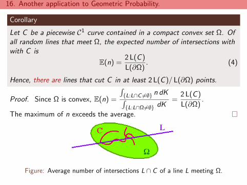
16. Another application to Geometric Probability.

Corollary

Let C be a piecewise C1 curve contained in a compact convex set Ω. Ofall random lines that meet Ω, the expected number of intersections withwith C is

E(n) =2 L(C )

L(∂Ω). (4)

Hence, there are lines that cut C in at least 2 L(C )/ L(∂Ω) points.

Proof. Since Ω is convex, E(n) =

∫L:L∩C 6=∅ n dK∫L:L∩Ω 6=∅ dK

=2 L(C )

L(∂Ω).

The maximum of n exceeds the average.

Figure: Average number of intersections L ∩ C of a line L meeting Ω.

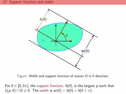
17. Support function and width.

Figure: Width and support function of convex Ω in θ direction.

For θ ∈ [0, 2π), the support function, h(θ), is the largest p such thatL(p, θ) ∩ Ω 6= ∅. The width is w(θ) = h(θ) + h(θ + π).

18. Another corollary: Mean projected width or Quermassintegral.

Figure: Augustin Louis Cauchy1789–1857

Theorem (Cauchy’s Formula [1841])

Let Ω be a bounded convex domain. Then

L(∂Ω) =

∫ 2π

0h(θ) dθ =

∫ π

0w(θ) dθ. (5)

L(∂Ω) =

∫L:L∩Ω 6=∅

dK =

∫ 2π

0

∫ h(θ)

0dp dθ

=

∫ 2π

0h(θ) dθ =

∫ π

0h(θ) + h(θ + π) dθ

=

∫ π

0w(θ) dθ.

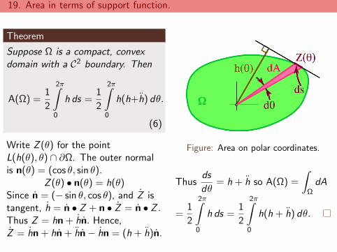
19. Area in terms of support function.

Theorem

Suppose Ω is a compact, convexdomain with a C2 boundary. Then

A(Ω) =1

2

2π∫0

h ds =1

2

2π∫0

h(h+h) dθ.

(6)

Write Z (θ) for the pointL(h(θ), θ) ∩ ∂Ω. The outer normalis n(θ) = (cos θ, sin θ).

Z (θ) • n(θ) = h(θ)Since n = (− sin θ, cos θ), and Z istangent, h = n • Z + n • Z = n • Z .Thus Z = hn + hn. Hence,Z = hn + hn + hn− hn = (h + h)n.

Figure: Area on polar coordinates.

Thusds

dθ= h + h so A(Ω) =

∫Ω

dA

=1

2

2π∫0

h ds =1

2

2π∫0

h(h + h) dθ.

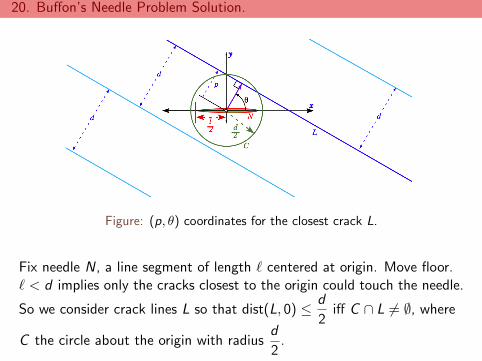
20. Buffon’s Needle Problem Solution.

Figure: (p, θ) coordinates for the closest crack L.

Fix needle N, a line segment of length ` centered at origin. Move floor.` < d implies only the cracks closest to the origin could touch the needle.

So we consider crack lines L so that dist(L, 0) ≤ d

2iff C ∩ L 6= ∅, where

C the circle about the origin with radiusd

2.

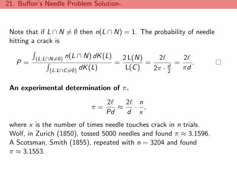
21. Buffon’s Needle Problem Solution-.

Note that if L ∩ N 6= ∅ then n(L ∩ N) = 1. The probability of needlehitting a crack is

P =

∫L:L∩N 6=∅ n(L ∩ N) dK (L)∫

L:L∩C 6=∅ dK (L)=

2 L(N)

L(C )=

2`

2π · d2

=2`

πd.

An experimental determination of π.

π =2`

Pd≈ 2`

d· n

x,

where x is the number of times needle touches crack in n trials.Wolf, in Zurich (1850), tossed 5000 needles and found π ≈ 3.1596.A Scotsman, Smith (1855), repeated with n = 3204 and foundπ ≈ 3.1553.

22. Crofton’s Formula.

Figure: Morgan WilliamCrofton 1826–1915.

Theorem (Crofton’s Formula [1868])

Let D ⊂ R2 be a domain with compactclosure, L ⊂ R2 a random line andσ1(L ∩ D) be the length (one-dimensionalmeasure). Then

π A(D) =

∫L:L∩D 6=∅

σ1(L ∩ D) dK (L).

Let the subset of the flag beS = (L,Z ) : L ∩ D 6= ∅, Z ∈ L ∩ D.A point in S is given by coordinates (p, θ)describing the line and q, arclength in Lfrom the foot point.

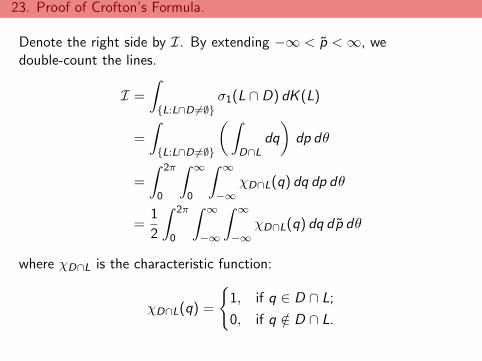
23. Proof of Crofton’s Formula.

Denote the right side by I. By extending −∞ < p <∞, wedouble-count the lines.

I =

∫L:L∩D 6=∅

σ1(L ∩ D) dK (L)

=

∫L:L∩D 6=∅

(∫D∩L

dq

)dp dθ

=

∫ 2π

0

∫ ∞

0

∫ ∞

−∞χD∩L(q) dq dp dθ

=1

2

∫ 2π

0

∫ ∞

−∞

∫ ∞


where χD∩L is the characteristic function:

χD∩L(q) =

1, if q ∈ D ∩ L;

0, if q /∈ D ∩ L.

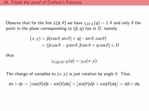
24. Finish the proof of Crofton’s Formula.

Observe that for the line L(p, θ) we have χD∩L(q) = 1 if and only if thepoint in the plane corresponding to (p, q) lies in D, namely

(x , y) = p(cos θ, sin θ) + q(− sin θ, cos θ)

= (p cos θ − q sin θ, p sin θ + q cos θ) ∈ D

thusχL(p,θ)∩D(q) = χD(x , y).

The change of variables to (x , y) is just rotation by angle θ. Thus

dx ∧ dy =[cos(θ)dp − sin(θ)dq

]∧[sin(θ)dp + cos(θ)dq

]= dp ∧ dq.

25. Finish the proof of Crofton’s Formula-.

Now we think of S another way. First pick Z ∈ D and then L is any linethrough Z .

I =1

2

∫ 2π

0

∫ ∞

−∞

∫ ∞


=1

2

∫ 2π

0

∫ ∞

−∞

∫ ∞

−∞χD(x , y) dx dy dθ

=1

2

∫ 2π

0A(D) dθ

= π A(D).

26. Application to Geometric Probability

Figure: Two random lines that meet Ω

Corollary (Crofton [1885])

Let Ω be a bounded convex domainin the plane. Then the probabilitythat two random lines intersect in Ωgiven that they both meet Ω is

P =2π A(Ω)

L(∂Ω)2.

By the isoperimetric inequality,4π A(Ω) ≤ L(∂Ω)2 with equalityonly for circle, the probabilitysatisfies

P ≤ 1

2.

Equality holds iff Ω is a round disk.

27. Compute the expected number of intersections of two lines.

Proof. Let L1(p1, θ1) and L2(p2, θ2) be two random lines whose invariantmeasure is dK1 ∧ dK2 = dp1 ∧ dθ1 ∧ dp2 ∧ dθ2.View Λ1 = L(p1, θ1) ∩ Ω as a subset. By (4), the average number oftimes that a random line L(p2, θ2) meets Λ1 given that it meets Ω is

E(n) =2σ1

(Ω ∩ L(p1, θ1)

)L(∂Ω)

.

Poincare’s and Crofton’s Formulæ =⇒ probability that two lines meet is

P = E(n) =

∫L1:L1∩Ω 6=∅

∫L2:L2∩Ω 6=∅ n(Λ1 ∩ L2) dK2 dK1∫

L1:L1∩Ω 6=∅∫L2:L2∩Ω 6=∅ dK2 dK1

=

∫L1:L1∩Ω 6=∅ E(n) dK1∫

L1:L1∩Ω 6=∅ dK1=

2∫L1:L1∩Ω 6=∅ σ1

(Ω ∩ L(p1, θ1)

)dK1

L(∂Ω)∫L1:L1∩∂Ω 6=∅ dK1

=2π A(Ω)

L(∂Ω)2.

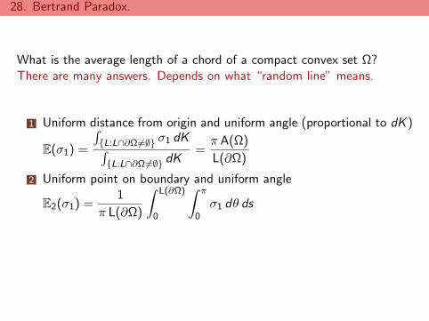
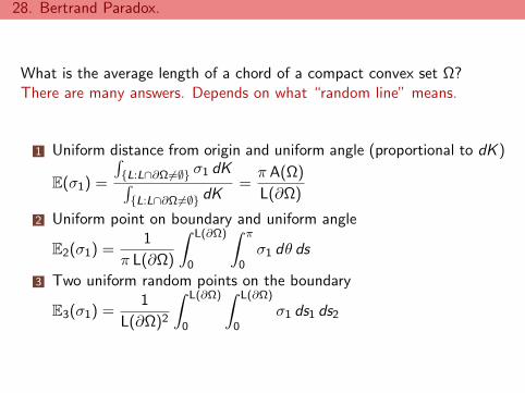
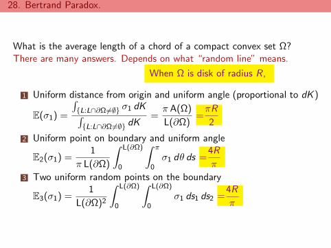
28. Bertrand Paradox.

What is the average length of a chord of a compact convex set Ω?

There are many answers. Depends on what “random line” means.

When Ω is disk of radius R,

1 Uniform distance from origin and uniform angle (proportional to dK )

E(σ1) =

∫L:L∩∂Ω 6=∅ σ1 dK∫L:L∩∂Ω 6=∅ dK

=π A(Ω)

L(∂Ω)=πR

2

2 Uniform point on boundary and uniform angle

E2(σ1) =1

π L(∂Ω)

∫ L(∂Ω)

0

∫ π

0σ1 dθ ds =

4R

π

3 Two uniform random points on the boundary

E3(σ1) =1

L(∂Ω)2

∫ L(∂Ω)

0

∫ L(∂Ω)

0σ1 ds1 ds2 =

4R

π


What is the average length of a chord of a compact convex set Ω?There are many answers. Depends on what “random line” means.



E(σ1) =

∫L:L∩∂Ω 6=∅ σ1 dK∫L:L∩∂Ω 6=∅ dK

=π A(Ω)

L(∂Ω)=πR

2


E2(σ1) =1

π L(∂Ω)

∫ L(∂Ω)

0

∫ π

0σ1 dθ ds =

4R

π


E3(σ1) =1

L(∂Ω)2

∫ L(∂Ω)

0

∫ L(∂Ω)

0σ1 ds1 ds2 =

4R

π





E(σ1) =

∫L:L∩∂Ω 6=∅ σ1 dK∫L:L∩∂Ω 6=∅ dK

=π A(Ω)

L(∂Ω)

=πR

2


E2(σ1) =1

π L(∂Ω)

∫ L(∂Ω)

0

∫ π

0σ1 dθ ds =

4R

π


E3(σ1) =1

L(∂Ω)2

∫ L(∂Ω)

0

∫ L(∂Ω)

0σ1 ds1 ds2 =

4R

π





E(σ1) =

∫L:L∩∂Ω 6=∅ σ1 dK∫L:L∩∂Ω 6=∅ dK

=π A(Ω)

L(∂Ω)

=πR

2


E2(σ1) =1

π L(∂Ω)

∫ L(∂Ω)

0

∫ π

0σ1 dθ ds

=4R

π


E3(σ1) =1

L(∂Ω)2

∫ L(∂Ω)

0

∫ L(∂Ω)

0σ1 ds1 ds2 =

4R

π





E(σ1) =

∫L:L∩∂Ω 6=∅ σ1 dK∫L:L∩∂Ω 6=∅ dK

=π A(Ω)

L(∂Ω)

=πR

2


E2(σ1) =1

π L(∂Ω)

∫ L(∂Ω)

0

∫ π

0σ1 dθ ds

=4R

π


E3(σ1) =1

L(∂Ω)2

∫ L(∂Ω)

0

∫ L(∂Ω)

0σ1 ds1 ds2

=4R

π





E(σ1) =

∫L:L∩∂Ω 6=∅ σ1 dK∫L:L∩∂Ω 6=∅ dK

=π A(Ω)

L(∂Ω)=πR

2


E2(σ1) =1

π L(∂Ω)

∫ L(∂Ω)

0

∫ π

0σ1 dθ ds =

4R

π


E3(σ1) =1

L(∂Ω)2

∫ L(∂Ω)

0

∫ L(∂Ω)

0σ1 ds1 ds2 =

4R

π

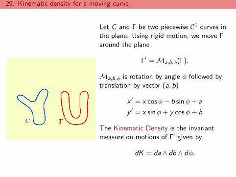
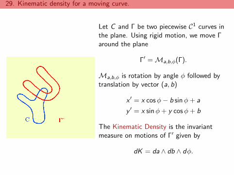
29. Kinematic density for a moving curve.

Let C and Γ be two piecewise C1 curves inthe plane. Using rigid motion, we move Γaround the plane

Γ′ = Ma,b,φ(Γ).

Ma,b,φ is rotation by angle φ followed bytranslation by vector (a, b)

x ′ = x cosφ− b sinφ+ a

y ′ = x sinφ+ y cosφ+ b

The Kinematic Density is the invariantmeasure on motions of Γ′ given by

dK = da ∧ db ∧ dφ.

















30. Poincare’s Formula.

Theorem (Poincare’s Formula for intersecting curves [1912])

Let C and Γ be piecewise C1 curves in the plane. Let n(C ∩ Γ′) denotethe number of intersection points between C and a moving Γ′. Then∫

Γ′:C∩Γ′ 6=∅

n(C ∩ Γ′) dK (Γ′) = 4 L(C ) L(Γ).

We show the formula for C1 curves and add to get it for piecewise C1

curves. We give two computations of the integral over the “flag” subset

S = (Γ′,X ) : C ∩ Γ′ 6= ∅, X ∈ C ∩ Γ′.

For simplicity, suppose the origin 0 ∈ C and 0 ∈ Γ.

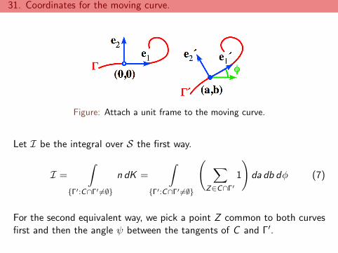
31. Coordinates for the moving curve.

Figure: Attach a unit frame to the moving curve.

Let I be the integral over S the first way.

I =

∫Γ′:C∩Γ′ 6=∅

n dK =

∫Γ′:C∩Γ′ 6=∅

( ∑Z∈C∩Γ′

1

)da db dφ (7)

For the second equivalent way, we pick a point Z common to both curvesfirst and then the angle ψ between the tangents of C and Γ′.

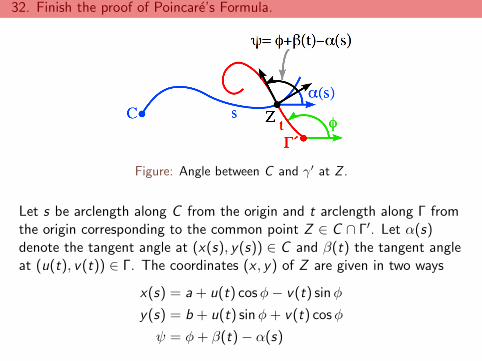
32. Finish the proof of Poincare’s Formula.

Figure: Angle between C and γ′ at Z .

Let s be arclength along C from the origin and t arclength along Γ fromthe origin corresponding to the common point Z ∈ C ∩ Γ′. Let α(s)denote the tangent angle at (x(s), y(s)) ∈ C and β(t) the tangent angleat (u(t), v(t)) ∈ Γ. The coordinates (x , y) of Z are given in two ways

x(s) = a + u(t) cosφ− v(t) sinφ

y(s) = b + u(t) sinφ+ v(t) cosφ

ψ = φ+ β(t)− α(s)

33. Finish the proof of Poincare’s Formula-.

Change to (s, t, ψ) coordinates for S. Differentiating the definingequations,

x(s) ds = da +[u(t) cosφ− v(t) sinφ

]dt −

[u(t) sinφ+ v(t) cosφ

]dφ

y(s) ds = db +[u(t) sinφ+ v(t) cosφ

]dt +

[u(t) cosφ− v(t) sinφ

]dφ

dψ = dφ+ β(t) dt − α(s) ds

Using (cosα, sinα) = (x , y) and (cosβ, sinβ) = (u, v), the kinematicdensity is thus da ∧ db ∧ dφ

=[x(s) ds −


]dt +


]dφ]

∧[y(s) ds −


]dt −


]dφ]

∧[dψ − β(t) dt + α(s) ds

]=(−x[u sinφ+ v cosφ

]+ y[u cosφ− v sinφ

])ds ∧ dt ∧ dψ

= − sin(ψ) ds ∧ dt ∧ dψ.

34. Finish the proof of Poincare’s Formula - -.

Using Fubini’s theorem, we find another expression for (7)

I =

∫C

∫Γ

2π∫0

da db dφ =

∫C

∫Γ

2π∫0

| sin(ψ)| dψ dt ds = 4L(C ) L(Γ).

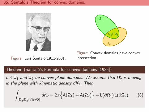
35. Santalo’s Theorem for convex domains.

Figure: Luis Santalo 1911-2001.

Figure: Convex domains have convexintersection.

Theorem (Santalo’s Formula for convex domains [1935])

Let Ω1 and Ω2 be convex plane domains. We assume that Ω′2 is moving

in the plane with kinematic density dK2. Then∫Ω′

2:Ω′2∩Ω1 6=∅

dK2 = 2π

A(Ω1) + A(Ω2)

+ L(∂Ω1) L(∂Ω2). (8)

36. Proof of Santalo’s Theorem.

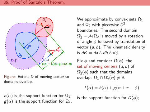
Figure: Extent D of moving center sodomains overlap.

h(α) is the support function for Ω1;g(α) is the support function for Ω2.

We approximate by convex sets Ω1

and Ω2 with piecewise C2

boundaries. The second domainΩ′

2 = MΩ2 is moved by a rotationof angle φ followed by translation ofvector (a, b). The kinematic densityis dK = da ∧ db ∧ dφ.

Fix φ and consider D(φ), theset of moving centers (a, b) ofΩ′

2(φ) such that the domainsoverlap: Ω1 ∩ Ω′

2(φ) 6= ∅.

f (α) = h(α) + g(α+ π − φ)

is the support function for D(φ);

37. Proof of Santalo’s Theorem -.

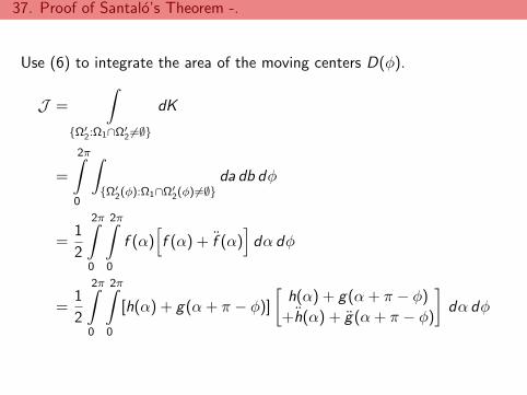
Use (6) to integrate the area of the moving centers D(φ).

J =

∫Ω′

2:Ω1∩Ω′2 6=∅

dK

=

2π∫0

∫Ω′

2(φ):Ω1∩Ω′2(φ) 6=∅

da db dφ

=1

2

2π∫0

2π∫0

f (α)[f (α) + f (α)

]dα dφ

=1

2

2π∫0

2π∫0

[h(α) + g(α+ π − φ)]

[h(α) + g(α+ π − φ)

+h(α) + g(α+ π − φ)

]dα dφ

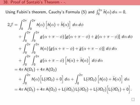
38. Proof of Santalo’s Theorem - -.

Using Fubini’s theorem, Cauchy’s Formula (5) and∫ 2π0 h(α) dα = 0,

2J =

∫ 2π

0

∫ 2π

0h(α)

[h(α) + h(α)

]dα dφ

+

∫ 2π

0

∫ 2π

0g(α+ π − φ) [g(α+ π − φ) + g(α+ π − φ)] dα dφ

+

∫ 2π

0

∫ 2π

0h(α) [g(α+ π − φ) + g(α+ π − φ)] dφ dα

+

∫ 2π

0

∫ 2π

0g(α+ π − φ)

[h(α) + h(α)

]dφ dα

= 4π A(Ω1) + 4π A(Ω2)

+

∫ 2π

0h(α)

[L(∂Ω2) + 0

]dα+

∫ 2π

0L(∂Ω2)

[h(α) + h(α)

]dα

= 4π A(Ω1) + 4π A(Ω2) + L(∂Ω1) L(∂Ω2) + L(∂Ω2)[L(∂Ω1) + 0

].

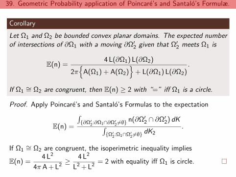
39. Geometric Probability application of Poincare’s and Santalo’s Formulæ.

Corollary

Let Ω1 and Ω2 be bounded convex planar domains. The expected numberof intersections of ∂Ω1 with a moving ∂Ω′

2 given that Ω′2 meets Ω1 is

E(n) =4 L(∂Ω1) L(∂Ω2)

2π

A(Ω1) + A(Ω2)

+ L(∂Ω1) L(∂Ω2).

If Ω1∼= Ω2 are congruent, then E(n) ≥ 2 with “=” iff Ω1 is a circle.

Proof. Apply Poincare’s and Santalo’s Formulas to the expectation

E(n) =

∫∂Ω′

2:∂Ω1∩∂Ω′2 6=∅

n(∂Ω′2 ∩ ∂Ω′

2) dK∫Ω′

2:Ω1∩Ω′2 6=∅

dK2.

If Ω1∼= Ω2 are congruent, the isoperimetric inequality implies

E(n) =4 L2

4π A+ L2≥ 4 L2

L2 +L2= 2 with equality iff Ω1 is circle.

40. Total curvature.

Let C be closed piecewise C2 curve.

The curvature is κ =∂α

∂s,

the rate of turning, where α givesthe angle via (cosα, sinα) = Z , thedirection of C at Z .

Figure: Piecewise C2 boundary withcorners at Zi

A piecewise C2 boundary is the

union of n curves ∂Ω =n⋃

i=1

Ci .

The total curvature is the integral ofthe curvatures over the C2 curves Ci

plus the turning angle at the verticesZi between Ci and Ci+1

c(∂Ω) =n∑

i=1

∫Ci

κ ds +n∑

i=1

αi

By the Gauss-Bonnet Formula, thetotal curvature of a boundary isrelated to the Euler Characteristic

c(∂Ω) = 2πχ(Ω).

41. Blaschke’s Theorem for general domains.

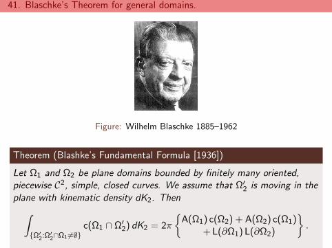
Figure: Wilhelm Blaschke 1885–1962

Theorem (Blashke’s Fundamental Formula [1936])

Let Ω1 and Ω2 be plane domains bounded by finitely many oriented,piecewise C2, simple, closed curves. We assume that Ω′

2 is moving in theplane with kinematic density dK2. Then∫

Ω′2:Ω

′2∩Ω1 6=∅

c(Ω1 ∩ Ω′2) dK2 = 2π

A(Ω1) c(Ω2) + A(Ω2) c(Ω1)

+L(∂Ω1) L(∂Ω2)

.

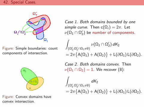
42. Special Cases.

Figure: Simple boundaries: countcomponents of intersection.

Figure: Convex domains haveconvex intersection.

Case 1. Both domains bounded by onesimple curve. Then c(Ωi ) = 2π. Letν(Ω1 ∩ Ω′

2) be number of components.∫Ω′

2:Ω′2∩Ω1 6=∅

ν(Ω1 ∩ Ω′2) dK2

= 2πA(Ω1) + A(Ω2)

+ L(∂Ω1) L(∂Ω2).

Case 2. Both domains convex. Thenν(Ω1 ∩ Ω2) = 1. We recover (8):∫Ω′

2:Ω′2∩Ω1 6=∅

dK2

= 2πA(Ω1) + A(Ω2)

+ L(∂Ω1) L(∂Ω2).

43. Isoperimetric Inequality - - An Integral Geometric Proof

Among all domains in the plane with a fixed boundary length, the circlehas the greatest area. For simplicity we focus on domains bounded bysimple curves.

Theorem (Isoperimetric Inequality.)

1 Let C be a simple closed curve in the plane whose length is L andthat encloses an area A. Then the following inequality holds

4πA ≤ L2. (9)

2 If equality holds in (9), then the curve C is a circle.

Simple means curve is assumed to have no self intersections.A circle of radius r has L = 2πr and encloses A = πr2 = L2

4π .Thus the isoperimetric Inequality says if C is a simple closed curve oflength L and encloses an area A, then C encloses an area no bigger thanthe area of the circle with the same length.

44. Convex Hull

A set K ⊂ E2 is convex if for every pair of points x , y ∈ K , the straightline segment xy from x to y is also in K , i.e., xy ⊂ K .The bounding curve of a convex set is automatically rectifiable. Theconvex hull of K , denoted K , is the smallest convex set that contains K .This is equivalent to the intersection of all halfspaces that contain K ,

K =⋂

Ω is convexΩ ⊃ K

Ω =⋂

H is a halfspaceH ⊃ K

H.

A halfspace is a set of the form H = (x , y) ∈ E2 : ax + by ≤ c, where(a, b) is a unit vector and c is any real number.

45. Reduce proof of Isoperimetric Inequality to convex domain case.

Since K ⊂ K by its definition, we have A(K ) ≥ A(K ).Taking convex hull reduces the boundary length because the interiorsegments of the boundary curve, the components of C − ∂K of C arereplaced by straight line segments in ∂K . Thus also L(∂K ) ≤ L(∂K ).

Figure: The region K and its convex hull K .

46. Reduce proof of Isoperimetric Inequality to convex curves case.-

Thus the isoperimetric inequality for convex sets implies

4πA ≤ 4πA ≤ L2 ≤ L2.

Furthermore, one may also argue that equality 4πA = L2 implies equality4πA = L2 in the isoperimetric inequality for convex sets so that K is acircle. But then so is K .

The basic idea is to consider the the extreme points ∂∗K ⊂ ∂K of K ,that is points x ∈ ∂K such that if x = λy + (1− λ)z for some y , z ∈ Kand 0 < λ < 1 then y = z = x . K is the convex hull of its extremepoints. However, the extreme points of the convex hull lie in the curve∂∗K ⊂ C ∩ ∂K . K being a circle implies that every boundary point is anextreme point, and since they come from C , it means that C is a circle.

47. Isoperimetric Inequality for convex sets

There are many proofs of the isoperimetric inequality. We shall give twointegral geometric arguments due to Luis Santalo.

1 The first argument only establishes the inequality part 4πA ≤ L2.

2 To show that the circle is the unique domain for which theIsoperimetric Inequality is equality, we prove a strong isoperimetricinequality (12) that follows from Bonnesen’s inequality (11). Thesecond argument is Santalo’s proof of Bonnesen’s inequality.

48. Santalo’s proof of the Isoperimetric Inequality for convex sets.

Lemma (Isoperimetric Inequality for convex sets.)

If Ω is a convex plane domain with boundary length L and area A, then

4πA ≤ L2. (10)

Proof. Let Ω1 and Ω2 be congruent copies of Ω. Let mi denote themeasure of positions of a moving Ω′

2 for which the number ofintersections

n(∂Ω1 ∩ ∂Ω′2) = i .

Note that positions that have an odd or infinite number of intersectionpoints is dK -measure zero so that

mi = 0 if i is odd.

49. Finish Santalo’s proof of the Isoperimetric Inequality.

Then by Poincare’s and Santalo’s formulas,

4 L(∂Ω)2 =

∫Ω′

2:∂Ω′2∩∂Ω1 6=∅

n(∂Ω1 ∩ ∂Ω′2) dK = 2m2 + 4m4 + 6m6 + · · · ,

4π A(Ω) + L(∂Ω)2 =

∫Ω′

2:Ω′2∩Ω1 6=∅

dK = m2 + m4 + m6 + · · · .

Subtracting,

L(∂Ω)2 − 4π A(Ω) = m4 + 2m6 + 3m8 + · · · ≥ 0,

since all the measures mi ≥ 0.

50. Inradius / Circumradius

Let K be the region bounded by γ. The radius of the smallest circulardisk containing K is called the circumradius, denoted Rout. The radius ofthe largest circular disk contained in K is the inradius.

Rin = supr : there is p ∈ E2 such that Br (p) ⊆ KRout = infr : there exists p ∈ E2 such that K ⊆ Br (p)

Figure: The disks realizing the circumradius, Rout, and inradius, Rin, of K .

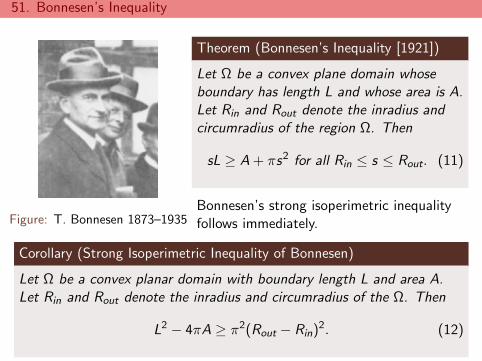
51. Bonnesen’s Inequality

Figure: T. Bonnesen 1873–1935

Theorem (Bonnesen’s Inequality [1921])

Let Ω be a convex plane domain whoseboundary has length L and whose area is A.Let Rin and Rout denote the inradius andcircumradius of the region Ω. Then

sL ≥ A + πs2 for all Rin ≤ s ≤ Rout. (11)

Bonnesen’s strong isoperimetric inequalityfollows immediately.

Corollary (Strong Isoperimetric Inequality of Bonnesen)

Let Ω be a convex planar domain with boundary length L and area A.Let Rin and Rout denote the inradius and circumradius of the Ω. Then

L2 − 4πA ≥ π2(Rout − Rin)2. (12)

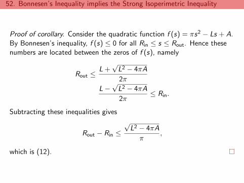
52. Bonnesen’s Inequality implies the Strong Isoperimetric Inequality

Proof of corollary. Consider the quadratic function f (s) = πs2 − Ls + A.By Bonnesen’s inequality, f (s) ≤ 0 for all Rin ≤ s ≤ Rout. Hence thesenumbers are located between the zeros of f (s), namely

Rout ≤L +

√L2 − 4πA

2π

L−√

L2 − 4πA

2π≤ Rin.

Subtracting these inequalities gives

Rout − Rin ≤√

L2 − 4πA

π,

which is (12).

53. Strong Isoperimetric Inequality implies the Isoperimetric Inequality

Obvious. The strong isoperimetric inequality (12) implies part one of theisoperimetric inequality (10), since π2(Rout − Rin)

2 ≥ 0.

Moreover, if equality holds in (9), then L2 − 4πA = 0 which implies thatRin = Rout, or Ω is a circle.

54. Santalo’s proof of Bonnesen’s inequality

Theorem (Bonnesen’s Inequality)

Let Ω be a bounded convex plane domain whose boundary has length Land whose area is A. Let Rin and Rout be the inradius and circumradiusof the region Ω. Then sL ≥ A + πs2 for all Rin ≤ s ≤ Rout.

Proof. Let Ω1 = Ω and Ω′2 be a moving circular disk of radius s.

Because Rin ≤ s ≤ Rout, the sets overlap, Ω1 ∩ Ω′2 6= ∅, if and only if

their boundaries overlap, ∂Ω1 ∩ ∂Ω′2 6= ∅, hence the Poincare and

Blaschke integrals are taken over the same positions of Ω′2.

As before, let mi denote the measure of positions of the moving Ω′2 for

which the number of intersections n(∂Ω1 ∩ ∂Ω′2) = i , i.e.,

mi = dK(

Ω′2 : n(∂Ω1 ∩ ∂Ω′

2) = i)

.

Again, positions that have an odd or infinite number of intersectionpoints is dK -measure zero so that mi = 0 if i is odd.

55. Finish Santalo’s proof of Bonnesen’s Inequality.

Then by Poincare’s and Santalo’s formulas,

8πs L(∂Ω) =

∫Ω′

2:Ω′2∩Ω1 6=∅

n(∂Ω1 ∩ ∂Ω′2) dK = 2m2 + 4m4 + 6m6 + · · · ,

2π A(Ω) + 2π2s2 + 2πs L(∂Ω) =

∫Ω′

2:Ω′2∩Ω1 6=∅

dK = m2 + m4 + m6 + · · · .

Subtracting,

2π(s L(∂Ω)− A(Ω)− πs2

)= m4 + 2m6 + 3m8 + · · · ≥ 0,

since all the measures mi ≥ 0.

Thanks!

Integral Geometry & Geometric Probabilitytreiberg/IntGeomSlides.pdf · Luis A. Santal´o, Integral Geometry and Geometric Probability, Addison-Wesley, Reading, MA, 1976. ... Figure:

Documents