Instructor’s Resource Manual Section 6.1 347 CHAPTER 6 Transcendental Functions 6.1 Concepts Review 1. 1 1 ; (0, ); (– , ) x dt t ∞ ∞∞ ∫ 2. 1 x 3. 1 ; ln x C x + 4. ln x + ln y; ln x – ln y; r ln x Problem Set 6.1 1. a. ln 6 = ln (2 · 3) = ln 2 + ln 3 = 0.693 + 1.099 = 1.792 b. 3 ln1.5 ln ln 3 ln 2 0.406 2 ⎛ ⎞ = = − = ⎜ ⎟ ⎝ ⎠ c. 4 ln 81 ln 3 4ln3 4(1.099) 4.396 = = = = d. 1/2 1 1 ln 2 ln 2 ln 2 (0.693) 0.3465 2 2 = = = = e. 2 2 1 ln – ln 36 – ln(2 3) 36 ⎛ ⎞ = = ⋅ ⎜ ⎟ ⎝ ⎠ 2 ln 2 2ln3 3.584 =− − =− f. 4 ln 48 ln(2 3) 4 ln 2 ln 3 3.871 = ⋅ = + = 2. a. 1.792 b. 0.405 c. 4.394 d. 0.3466 e. –3.584 f. 3.871 3. 2 ln( 3 ) x D x x + +π 2 2 1 ( 3 ) 3 x D x x x x = ⋅ + +π + +π 2 2 3 3 x x x + = + +π 4. 3 3 3 1 ln(3 2) (3 2) 3 2 x x D x x D x x x x + = + + 2 3 9 2 3 2 x x x + = + 5. 3 ln( – 4) 3ln( – 4) x x D x D x = 1 3 3 ( – 4) – 4 –4 x D x x x = ⋅ = 6. 1 ln 3 –2 ln(3 – 2) 2 x x D x D x = 1 1 3 (3 – 2) 23 –2 2(3 – 2) x D x x x = ⋅ = 7. 1 3 3 dy dx x x = ⋅ = 8. 2 1 2 ln dy x x x dx x = ⋅ + ⋅ = x(1 + 2 ln x) 9. 2 2 3 ln (ln ) z x x x = + 2 3 2 ln (ln ) x x x = ⋅ + 2 2 2 1 2 2 ln 3(ln ) dz x x x x dx x x = ⋅ + ⋅ + ⋅ 2 3 2 4 ln (ln ) x x x x x = + + 10. 3 2 2 ln 1 ln ln x r x x x ⎛ ⎞ = + ⎜ ⎟ ⎝ ⎠ 3 2 ln (– ln ) 2 ln x x x x = + ⋅ –2 3 1 – (ln ) 2 x x = –3 2 –2 1 – 3(ln ) 2 dr x x dx x = ⋅ 2 3 1 3(ln ) x x x =− − 11. 2 –1/2 2 1 1 () 1 ( 1) 2 2 1 g x x x x x ⎡ ⎤ ′ = + + ⋅ ⎢ ⎥ ⎣ ⎦ + + 2 1 1 x = + 12. 2 –1/2 2 1 1 () 1 ( – 1) 2 2 –1 h x x x x x ⎡ ⎤ ′ = + ⋅ ⎢ ⎥ ⎣ ⎦ + 2 1 1 x = − 13. 3 1 () ln ln 3 f x x x = = 11 1 () 3 3 f x x x ′ = ⋅ = 1 1 (81) 3 81 243 f ′ = = ⋅ 14. 1 () (– sin ) – tan cos f x x x x ′ = = tan 1 4 4 f π π ⎛ ⎞ ⎛ ⎞ ′ = − =− ⎜ ⎟ ⎜ ⎟ ⎝ ⎠ ⎝ ⎠ .

Welcome message from author
This document is posted to help you gain knowledge. Please leave a comment to let me know what you think about it! Share it to your friends and learn new things together.
Transcript
Instructor’s Resource Manual Section 6.1 347
CHAPTER 6 Transcendental Functions
6.1 Concepts Review
1. 1
1 ; (0, ); (– , )x
dtt
∞ ∞ ∞∫
2. 1x
3. 1 ; ln x Cx
+
4. ln x + ln y; ln x – ln y; r ln x
Problem Set 6.1
1. a. ln 6 = ln (2 · 3) = ln 2 + ln 3 = 0.693 + 1.099 = 1.792
b. 3ln1.5 ln ln 3 ln 2 0.4062
⎛ ⎞= = − =⎜ ⎟⎝ ⎠
c. 4ln 81 ln 3 4ln 3 4(1.099) 4.396= = = =
d. 1/ 2 1 1ln 2 ln 2 ln 2 (0.693) 0.34652 2
= = = =
e. 2 21ln – ln 36 – ln(2 3 )36
⎛ ⎞ = = ⋅⎜ ⎟⎝ ⎠
2 ln 2 2ln 3 3.584= − − = −
f. 4ln 48 ln(2 3) 4ln 2 ln 3 3.871= ⋅ = + =
2. a. 1.792 b. 0.405
c. 4.394 d. 0.3466
e. –3.584 f. 3.871
3. 2ln( 3 )xD x x+ + π
22
1 ( 3 )3
xD x xx x
= ⋅ + + π+ + π 2
2 33
xx x
+=
+ + π
4. 3 331ln(3 2 ) (3 2 )
3 2x xD x x D x x
x x+ = +
+
2
39 23 2
xx x
+=
+
5. 3ln( – 4) 3ln( – 4)x xD x D x= 1 33 ( – 4)– 4 – 4xD x
x x= ⋅ =
6. 1ln 3 – 2 ln(3 – 2)2x xD x D x=
1 1 3(3 – 2)2 3 – 2 2(3 – 2)xD x
x x= ⋅ =
7. 1 33dydx x x
= ⋅ =
8. 2 1 2 lndy x x xdx x
= ⋅ + ⋅ = x(1 + 2 ln x)
9. 2 2 3ln (ln )z x x x= + 2 32 ln (ln )x x x= ⋅ +
2 22 12 2ln 3(ln )dz x x x xdx x x
= ⋅ + ⋅ + ⋅
232 4 ln (ln )x x x xx
= + +
10. 3
2 2ln 1lnln
xrxx x
⎛ ⎞= + ⎜ ⎟⎝ ⎠
32
ln (– ln )2 ln
x xx x
= +⋅
–2 31 – (ln )2
x x=
–3 2–2 1– 3(ln )2
dr x xdx x
= ⋅ 2
31 3(ln )x
xx= − −
11. 2 –1/ 22
1 1( ) 1 ( 1) 221
g x x xx x
⎡ ⎤′ = + + ⋅⎢ ⎥⎣ ⎦+ +
2
1
1x=
+
12. 2 –1/ 22
1 1( ) 1 ( –1) 22–1
h x x xx x
⎡ ⎤′ = + ⋅⎢ ⎥⎣ ⎦+
2
1
1x=
−
13.
3 1( ) ln ln
3f x x x= =
1 1 1( )3 3
f xx x
′ = ⋅ =
1 1(81)3 81 243
f ′ = =⋅
14. 1( ) (– sin ) – tancos
f x x xx
′ = =
tan 14 4
f π π⎛ ⎞ ⎛ ⎞′ = − = −⎜ ⎟ ⎜ ⎟⎝ ⎠ ⎝ ⎠
.
348 Section 6.1 Instructor’s Resource Manual
15. Let u = 2x + 1 so du = 2 dx. 1 1 1
2 1 2dx du
x u=
+∫ ∫
1 1ln ln 2 12 2
u C x C= + = + +
16. Let u = 1 – 2x so du = –2dx. 1 1 1–
1– 2 2dx du
x u=∫ ∫
1 1– ln – ln 1– 22 2
u C x C= + = +
17. Let 23 9u v v= + so du = 6v + 9.
26 9 1 ln
3 9v dv du u C
uv v+
= = ++∫ ∫
2ln 3 9v v C= + +
18. Let 22 8u z= + so du = 4z dz.
21 142 8
z dz duuz
=+∫ ∫
( )21 1ln ln 2 84 4
u C z C= + = + +
19. Let u = ln x so 1du dxx
=
2 ln 2x dx udux
=∫ ∫
2 2(ln )u C x C= + = +
20. Let u = ln x, so 1du dxx
= .
–22
–1 –(ln )
dx u dux x
=∫ ∫
1 1ln
C Cu x
= + = +
21. Let 52u x= + π so 410du x dx= . 4
51 1
102x dx du
ux=
+ π∫ ∫
51 1ln ln 210 10
u C x C= + = + π +
343 550 0
1 ln 2102
x dx xx
⎡ ⎤= + π⎢ ⎥⎣ ⎦+ π∫
1 [ln(486 ) – ln ]10
= + π π = 10 486ln 0.5048+ π≈
π
22. Let 22 4 3u t t= + + so (4 4)du t dt= + .
21 1 1
42 4 3t dt du
ut t+
=+ +∫ ∫
21 1ln ln 2 4 34 4
u C t t= + = + + + C
11 220 0
1 1 ln 2 4 342 4 3
t dt t tt t
+ ⎡ ⎤= + +⎢ ⎥⎣ ⎦+ +∫
441 1 9ln 9 – ln 3 ln ln 34 4 3
= = = = 1 ln 34
23. By long division, 2 111 1
x xx x
= + +− −
so 2
2
111 1
ln 12
x dx x dx dx dxx x
x x x C
= + +− −
= + + − +
∫ ∫ ∫ ∫
24. By long division, 2 3 3
2 1 2 4 4(2 1)x x x
x x+
= + +− −
so
2
2
3 32 1 2 4 4(2 1)
3 3 14 4 4 2 1
x x xdx dx dx dxx x
x x dxx
+= + +
− −
= + +−
∫ ∫ ∫ ∫
∫Let 2 1u x= − ; then 2du dx= . Hence
1 1 1 1 ln2 1 2 2
1 ln 2 12
dx du u Cx u
x C
= = +−
= − +
∫ ∫
and 2 2 3 3 ln 2 1
2 1 4 4 8x x xdx x x C
x+
= + + − +−∫
25. By long division, 4
3 2 2564 16 644 4
x x x xx x
= − + − ++ +
so
4
3 2
4 32
414 16 64 256
44 8 64 256ln 4
4 3
x dxx
x dx x dx xdx dx dxx
x x x x x C
=+
− + − ++
= − + − + + +
∫
∫ ∫ ∫ ∫ ∫
26. By long division, 3 2
2 422 2
x x x xx x
+= − + −
+ + so
3 22
3 2
12 42 2
2 4ln 23 2
x x dx x dx xdx dx dxx x
x x x x C
+= − + −
+ +
= − + − + +
∫ ∫ ∫ ∫ ∫
Instructor’s Resource Manual Section 6.1 349
27. 22 ln( 1) – ln ln( 1) – lnx x x x+ = +2( 1)ln x
x+
=
28. 1 1ln( – 9) ln ln – 9 – ln2 2
x x x x+ =
– 9 – 9ln lnx xxx
= =
29. ln(x – 2) – ln(x + 2) + 2 ln x
2ln( – 2) – ln( 2) lnx x x= + +2 ( – 2)ln
2x x
x=
+
30. 2ln( – 9) – 2ln( – 3) – ln( 3)x x x + 2 2ln( 9) ln( 3) ln( 3)x x x= − − − − +
2
2– 9ln
( – 3) ( 3)x
x x=
+ 1ln
– 3x=
31. 31ln ln( 11) – ln( – 4)2
y x x= +
23
1 1 1 11– 311 2 – 4
dy xy dx x x
= ⋅ ⋅ ⋅+
2
31 3–11 2( – 4)
xx x
=+
2
31 3–11 2( – 4)
dy xydx x x
⎡ ⎤= ⋅ ⎢ ⎥
+⎢ ⎥⎣ ⎦
2
33
11 1 3–11 2( – 4)– 4
x xx xx
⎡ ⎤+= ⎢ ⎥
+⎢ ⎥⎣ ⎦
3 2
3 3/ 233 8–
2( – 4)x x
x+ +
=
32. 2 2ln ln( 3 ) ln( – 2) ln( 1)y x x x x= + + + +
2 21 2 3 1 2
– 23 1dy x x
y dx xx x x+
= + ++ +
2 22 2
2 3 1 2( 3 )( – 2)( 1)– 23 1
dy x xx x x xdx xx x x
+⎛ ⎞= + + + +⎜ ⎟
+ +⎝ ⎠4 3 25 4 –15 2 – 6x x x x= + +
33. 1 1ln ln( 13) – ln( – 4) – ln(2 1)2 3
y x x x= + +
1 1 1 2– –2( 13) – 4 3(2 1)
dyy dx x x x
=+ +
313 1 1 2– –
2( 13) – 4 3(2 1)( – 4) 2 1dy xdx x x xx x
⎡ ⎤+= ⎢ ⎥+ ++ ⎣ ⎦
2
2 1/ 2 4 / 310 219 –118–
6( – 4) ( 13) (2 1)x x
x x x+
=+ +
34. 22 1ln ln( 3) 2 ln(3 2) – ln( 1)3 2
y x x x= + + + +
21 2 2 2 3 1–
3 3 2 2( 1)3dy x
y dx x xx⋅
= ⋅ ++ ++
2 2 / 3 2
2( 3) (3 2) 4 6 1–
3 2 2( 1)1 3( 3)dy x x xdx x xx x
⎡ ⎤+ += +⎢ ⎥
+ ++ +⎢ ⎥⎣ ⎦
3 2
2 1/ 3 3 / 2(3 2)(51 70 97 90)
6( 3) ( 1)x x x x
x x+ + + +
=+ +
35.
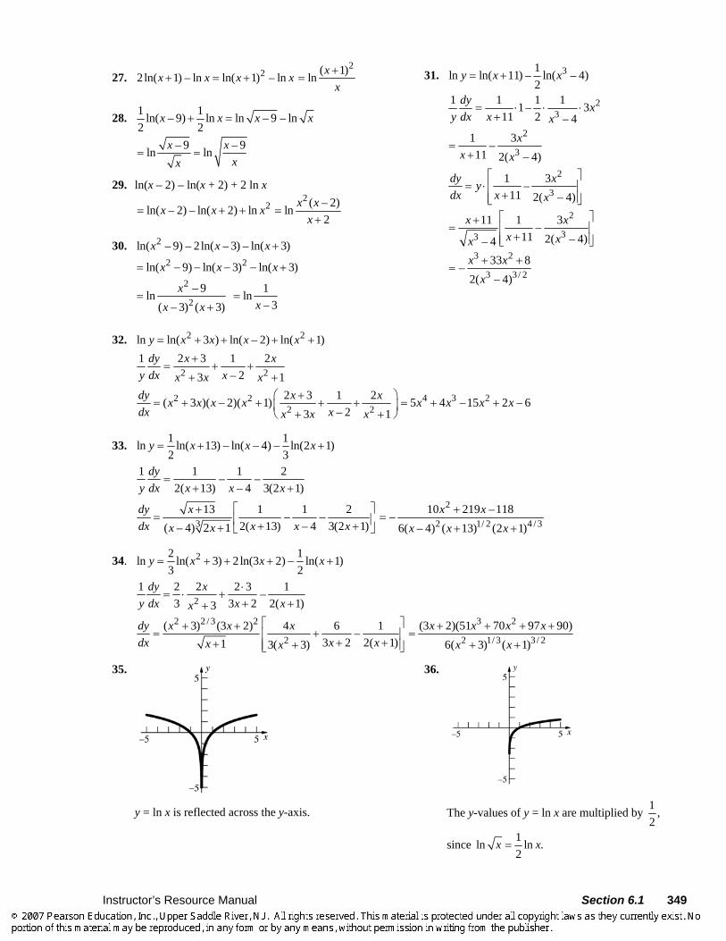
y = ln x is reflected across the y-axis.
36.
The y-values of y = ln x are multiplied by 1 ,2
since 1ln ln .2
x x=
350 Section 6.1 Instructor’s Resource Manual
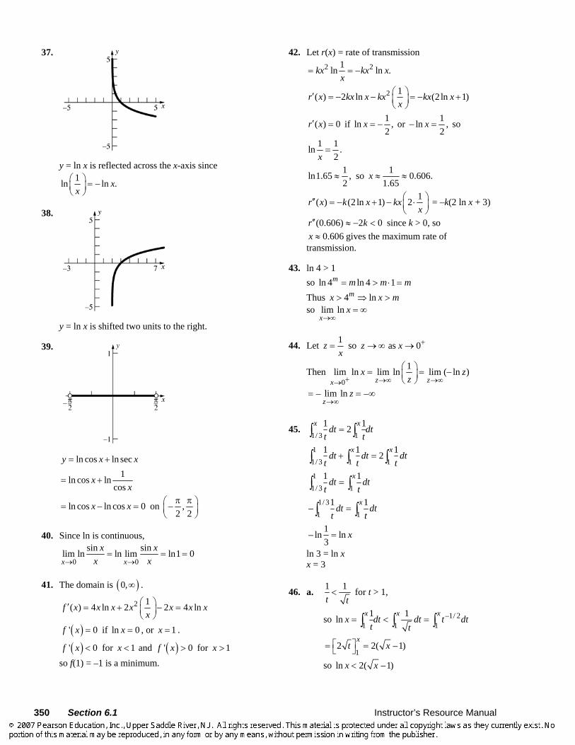
37.
y = ln x is reflected across the x-axis since 1ln – ln .xx
⎛ ⎞ =⎜ ⎟⎝ ⎠
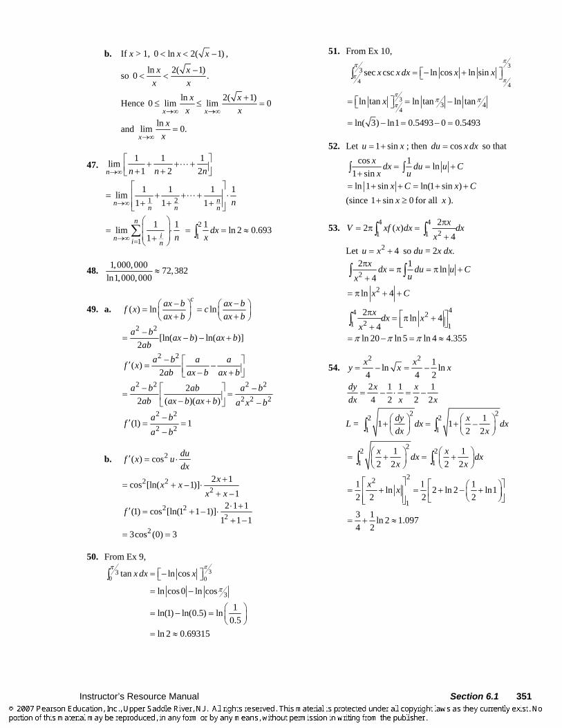
38.
y = ln x is shifted two units to the right.
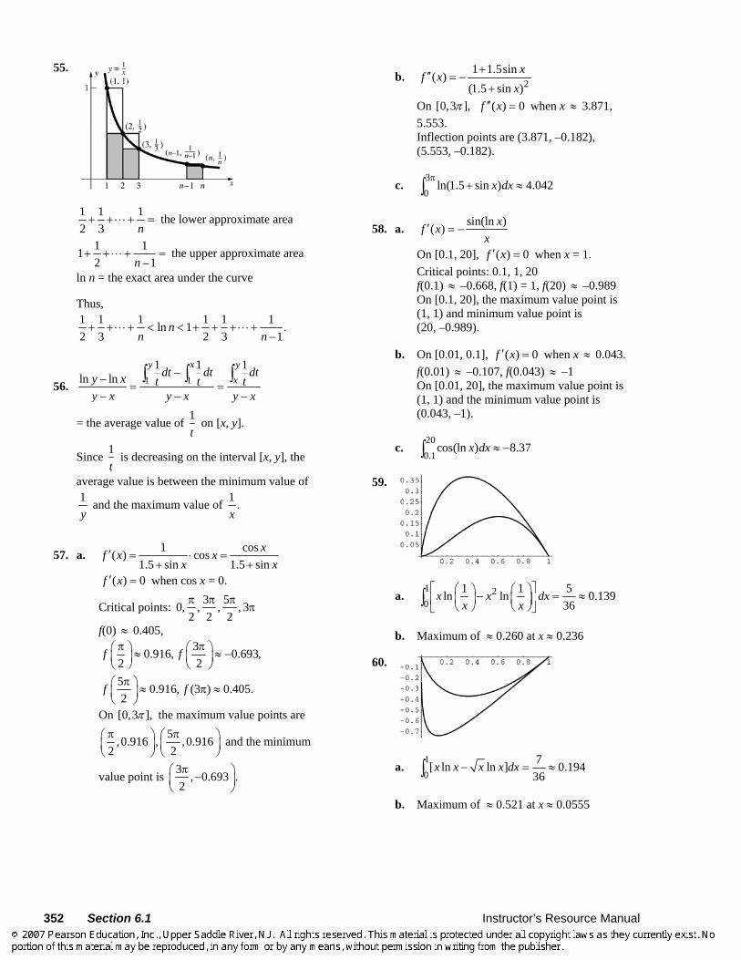
39.
ln cos ln secy x x= + 1ln cos ln
cosx
x= +
ln cos ln cos 0x x= − = on , 2 2π π⎛ ⎞−⎜ ⎟
⎝ ⎠
40. Since ln is continuous,
0 0
sin sinlim ln ln lim ln1 0x x
x xx x→ →
= = =
41. The domain is ( )0,∞ .
2 1( ) 4 ln 2 2 4 lnf x x x x x x xx
⎛ ⎞′ = + − =⎜ ⎟⎝ ⎠
( )' 0f x = if ln 0x = , or 1x = .
( )' 0f x < for 1x < and ( )' 0f x > for 1x > so f(1) = –1 is a minimum.
42. Let r(x) = rate of transmission 2 21ln ln .kx kx x
x= = −
2 1( ) 2 ln (2 ln 1)r x kx x kx kx xx
⎛ ⎞′ = − − = − +⎜ ⎟⎝ ⎠
( ) 0r x′ = if 1ln ,2
x = − or 1ln ,2
x− = so
1 1ln .2x
=
1ln1.65 ,2
≈ so 1 0.606.1.65
x ≈ ≈
1( ) (2 ln 1) 2r x k x kxx
⎛ ⎞′′ = − + − ⋅⎜ ⎟⎝ ⎠
= –k(2 ln x + 3)
(0.606) 2 0r k′′ ≈ − < since k > 0, so 0.606x ≈ gives the maximum rate of
transmission.
43. ln 4 > 1 so ln 4 ln 4 1m m m m= > ⋅ = Thus 4 lnmx x m> ⇒ > so lim ln
xx
→∞= ∞
44. Let 1zx
= so as 0z x +→ ∞ →
Then 0
1lim ln lim ln lim (– ln )z zx
x zz+ →∞ →∞→
⎛ ⎞= =⎜ ⎟⎝ ⎠
– lim ln –z
z→∞
= = ∞
45. 1/ 3 1
1 12x x
dt dtt t
=∫ ∫
11/ 3 1 1
1 1 12x x
dt dt dtt t t
+ =∫ ∫ ∫
11/ 3 1
1 1xdt dt
t t=∫ ∫
1/ 31 1
1 1–x
dt dtt t
=∫ ∫
1– ln ln3
x=
ln 3 = ln x x = 3
46. a. 1 1t t
< for t > 1,
so –1/ 21 1 1
1 1lnx x x
x dt dt t dtt t
= < =∫ ∫ ∫
12 2( –1)
xt x⎡ ⎤= =⎣ ⎦
so ln 2( –1)x x<
Instructor’s Resource Manual Section 6.1 351
b. If x > 1, 0 ln 2( –1)x x< < ,
so ln 2( –1)0 .x xx x
< <
Hence ln 2( 1)0 lim lim 0x x
x xx x→∞ →∞
+≤ ≤ =
and lnlim 0.x
xx→∞
=
47.
1 2
1 1 1lim1 2 2
1 1 1 1lim1 1 1
n
nn n n n
n n n
n
→∞
→∞
⎡ ⎤+ + ⋅⋅ ⋅ +⎢ ⎥+ +⎣ ⎦⎡ ⎤⎢ ⎥= + + ⋅⋅ ⋅ + ⋅
+ + +⎢ ⎥⎣ ⎦
1
1 1lim1
n
in i nn→∞ =
⎛ ⎞⎜ ⎟= ⋅⎜ ⎟+⎝ ⎠
∑ 2
11 ln 2 0.693dxx
= = ≈∫
48. 1,000,000 72,382ln1,000,000
≈
49. a. –( ) ln lncax b ax bf x c
ax b ax b−⎛ ⎞ ⎛ ⎞= =⎜ ⎟ ⎜ ⎟+ +⎝ ⎠ ⎝ ⎠
2 2– [ln( – ) – ln( )]2
a b ax b ax bab
= +
2 2–( ) –2 –
a b a af xab ax b ax b
⎡ ⎤′ = ⎢ ⎥+⎣ ⎦
2 2 2 2
2 2 22 –
2 ( )( ) –a b ab a b
ab ax b ax b a x b⎡ ⎤−
= =⎢ ⎥− +⎣ ⎦
2 2
2 2(1) 1a bfa b
−′ = =−
b. 2( ) cos duf x udx
′ = ⋅
2 222 1cos [ln( –1)]
–1xx x
x x+
= + ⋅+
2 222 1 1(1) cos [ln(1 1–1)]
1 1–1f ⋅ +′ = + ⋅
+23cos (0) 3= =
50. From Ex 9, 3
0 03
3
tan ln cos
ln cos 0 ln cos
1ln(1) ln(0.5) ln0.5
ln 2 0.69315
x dx xππ
π
= ⎡− ⎤⎣ ⎦
= −
⎛ ⎞= − = ⎜ ⎟⎝ ⎠
= ≈
∫
51. From Ex 10, 3
4 4
3
4
3
3 4
sec csc ln cos ln sin
ln tan ln tan ln tan
ln( 3) ln1 0.5493 0 0.5493
x x dx x x
x
π
π π
π
π
π
π π
= ⎡− + ⎤⎣ ⎦
= ⎡ ⎤ = −⎣ ⎦
= − = − =
∫
52. Let 1 sinu x= + ; then cosdu x dx= so that cos 1 ln
1 sinln 1 sin ln(1 sin )
x dx du u Cx u
x C x C
= = ++
= + + = + +
∫ ∫
(since 1 sin 0x+ ≥ for all x ).
53. 4 4
21 122 ( )
4xV xf x dx dx
xπ
= π =+∫ ∫
Let 2 4u x= + so du = 2x dx.
22 1 ln
4x dx du u C
uxπ
= π = π ++∫ ∫
2ln 4x C= π + +
44 221 1
2 ln 44
x dx xx
π ⎡ ⎤= π +⎢ ⎥⎣ ⎦+∫
ln 20 ln 5 ln 4 4.355π π π= − = ≈
54. 2 2 1– ln – ln
4 4 2x xy x x= =
2 1 1 1– –4 2 2 2
dy x xdx x x
= ⋅ =
L = 2 22 2
1 111 1 –
2 2dy xdx dxdx x
⎛ ⎞ ⎛ ⎞+ = +⎜ ⎟ ⎜ ⎟⎝ ⎠ ⎝ ⎠∫ ∫
22 21 1
1 12 2 2 2x xdx dx
x x⎛ ⎞ ⎛ ⎞= + = +⎜ ⎟ ⎜ ⎟⎝ ⎠ ⎝ ⎠∫ ∫
22
1
1 1ln 2 ln 2 ln12 2 2 2
x x⎡ ⎤ 1 ⎡ ⎤⎛ ⎞= + = + − +⎢ ⎥ ⎜ ⎟⎢ ⎥⎝ ⎠⎣ ⎦⎢ ⎥⎣ ⎦
3 1 ln 2 1.0974 2
= + ≈
352 Section 6.1 Instructor’s Resource Manual
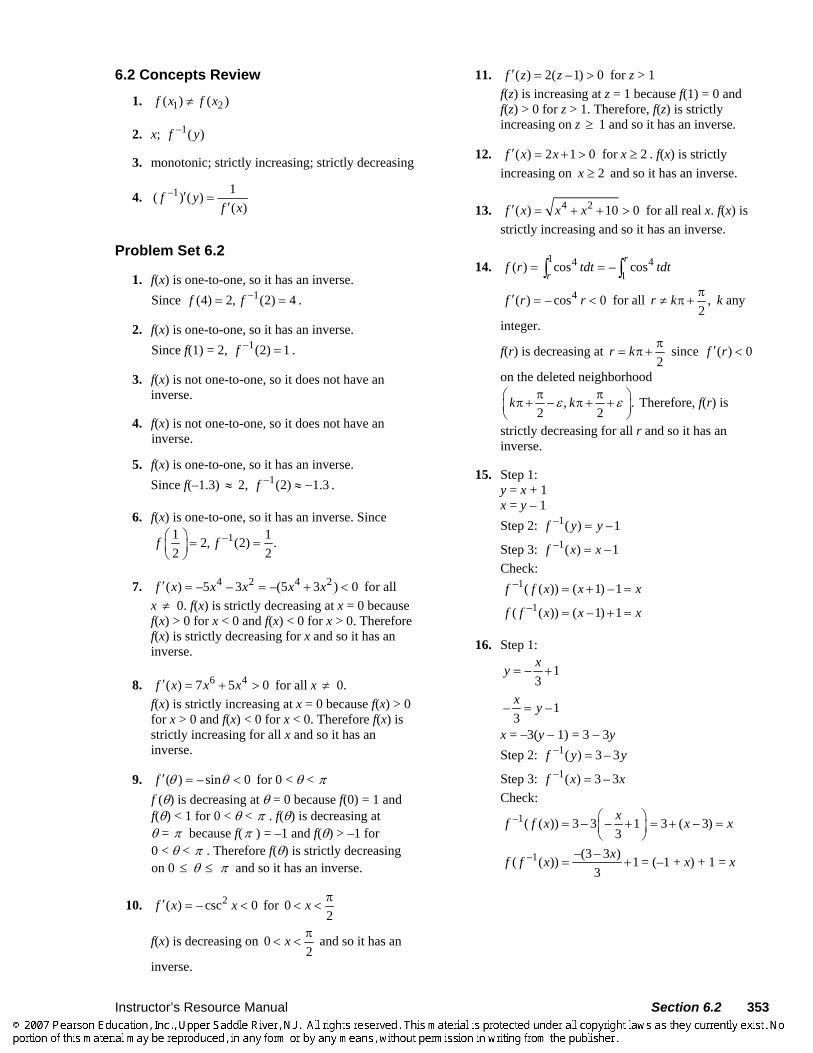
1 1 12 3 n
+ + ⋅⋅⋅ + = the lower approximate area
1 112 –1n
+ + ⋅⋅ ⋅ + = the upper approximate area
ln n = the exact area under the curve
Thus, 1 1 1 1 1 1ln 1 .2 3 2 3 1
nn n
+ + ⋅⋅ ⋅ + < < + + + ⋅⋅ ⋅ +−
56. 1 11 1 1–ln – ln
– – –
y x yx
dt dt dty x t t ty x y x y x
= =∫ ∫ ∫
= the average value of 1t
on [x, y].
Since 1t
is decreasing on the interval [x, y], the
average value is between the minimum value of
1y
and the maximum value of 1 .x
57. a. 1 cos( ) cos1.5 sin 1.5 sin
xf x xx x
′ = ⋅ =+ +
( ) 0f x′ = when cos x = 0.
Critical points: 3 50, , , , 32 2 2π π π
π
f(0) ≈ 0.405, 30.916, 0.693,
2 2f fπ π⎛ ⎞ ⎛ ⎞≈ ≈ −⎜ ⎟ ⎜ ⎟
⎝ ⎠ ⎝ ⎠
5 0.916, (3 ) 0.405.2
f fπ⎛ ⎞ ≈ π ≈⎜ ⎟⎝ ⎠
On [0,3 ],π the maximum value points are 5,0.916 , ,0.916
2 2π π⎛ ⎞ ⎛ ⎞
⎜ ⎟ ⎜ ⎟⎝ ⎠ ⎝ ⎠
and the minimum
value point is 3 , 0.693 .2π⎛ ⎞−⎜ ⎟
⎝ ⎠
b. 21 1.5sin( )
(1.5 sin )xf x
x+′′ = −
+
On [0,3 ],π ( ) 0f x′′ = when x ≈ 3.871, 5.553. Inflection points are (3.871, –0.182), (5.553, –0.182).
c. 30
ln(1.5 sin ) 4.042x dxπ
+ ≈∫
58. a. sin(ln )( ) xf xx
′ = −
On [0.1, 20], ( ) 0f x′ = when x = 1. Critical points: 0.1, 1, 20 f(0.1) ≈ –0.668, f(1) = 1, f(20) ≈ –0.989 On [0.1, 20], the maximum value point is (1, 1) and minimum value point is (20, –0.989).
b. On [0.01, 0.1], ( ) 0f x′ = when x ≈ 0.043. f(0.01) ≈ –0.107, f(0.043) ≈ –1 On [0.01, 20], the maximum value point is (1, 1) and the minimum value point is (0.043, –1).
c. 200.1
cos(ln ) 8.37x dx ≈ −∫
59.
a. 1 20
1 1 5ln ln 0.13936
x x dxx x
⎡ ⎤⎛ ⎞ ⎛ ⎞− = ≈⎜ ⎟ ⎜ ⎟⎢ ⎥⎝ ⎠ ⎝ ⎠⎣ ⎦∫
b. Maximum of ≈ 0.260 at x ≈ 0.236
60.
a. 10
7[ ln ln ] 0.19436
x x x x dx− = ≈∫
b. Maximum of ≈ 0.521 at x ≈ 0.0555
55.
Instructor’s Resource Manual Section 6.2 353
6.2 Concepts Review
1. 1 2( ) ( )f x f x≠
2. x; –1( )f y
3. monotonic; strictly increasing; strictly decreasing
4. –1 1( ) ( )( )
f yf x
′ =′
Problem Set 6.2
1. f(x) is one-to-one, so it has an inverse. Since 1(4) 2, (2) 4f f −= = .
2. f(x) is one-to-one, so it has an inverse. Since f(1) = 2, 1(2) 1f − = .
3. f(x) is not one-to-one, so it does not have an inverse.
4. f(x) is not one-to-one, so it does not have an inverse.
5. f(x) is one-to-one, so it has an inverse. Since f(–1.3) ≈ 2, 1(2) 1.3f − ≈ − .
6. f(x) is one-to-one, so it has an inverse. Since 11 12, (2) .
2 2f f −⎛ ⎞ = =⎜ ⎟
⎝ ⎠
7. 4 2 4 2( ) –5 – 3 –(5 3 ) 0f x x x x x′ = = + < for all x ≠ 0. f(x) is strictly decreasing at x = 0 because f(x) > 0 for x < 0 and f(x) < 0 for x > 0. Therefore f(x) is strictly decreasing for x and so it has an inverse.
8. 6 4( ) 7 5 0f x x x′ = + > for all x ≠ 0. f(x) is strictly increasing at x = 0 because f(x) > 0 for x > 0 and f(x) < 0 for x < 0. Therefore f(x) is strictly increasing for all x and so it has an inverse.
9. ( ) – sin 0f θ θ′ = < for 0 < θ < π f (θ) is decreasing at θ = 0 because f(0) = 1 and f(θ) < 1 for 0 < θ < π . f(θ) is decreasing at θ = π because f(π ) = –1 and f(θ) > –1 for 0 < θ < π . Therefore f(θ) is strictly decreasing on 0 ≤ θ ≤ π and so it has an inverse.
10. 2( ) – csc 0f x x′ = < for 02
x π< <
f(x) is decreasing on 02
x π< < and so it has an
inverse.
11. ( ) 2( –1) 0f z z′ = > for z > 1 f(z) is increasing at z = 1 because f(1) = 0 and f(z) > 0 for z > 1. Therefore, f(z) is strictly increasing on z ≥ 1 and so it has an inverse.
12. ( ) 2 1 0f x x′ = + > for 2x ≥ . f(x) is strictly increasing on 2x ≥ and so it has an inverse.
13. 4 2( ) 10 0f x x x′ = + + > for all real x. f(x) is strictly increasing and so it has an inverse.
14. 1 4 4
1( ) cos – cos
rr
f r tdt tdt= =∫ ∫
4( ) – cos 0f r r′ = < for all ,2
r k π≠ π + k any
integer.
f(r) is decreasing at 2
r k π= π + since ( ) 0f r′ <
on the deleted neighborhood
, .2 2
k kε επ π⎛ ⎞π + − π + +⎜ ⎟⎝ ⎠
Therefore, f(r) is
strictly decreasing for all r and so it has an inverse.
15. Step 1: y = x + 1 x = y – 1 Step 2: –1( ) –1f y y=
Step 3: –1( ) –1f x x= Check:
–1( ( )) ( 1) –1f f x x x= + = –1( ( )) ( –1) 1f f x x x= + =
16. Step 1:
– 13xy = +
– –13x y=
x = –3(y – 1) = 3 – 3y Step 2: –1( ) 3 – 3f y y=
Step 3: –1( ) 3 – 3f x x= Check:
–1( ( )) 3 – 3 – 13xf f x ⎛ ⎞= +⎜ ⎟
⎝ ⎠3 ( – 3)x x= + =
–1 –(3 – 3 )( ( )) 13
xf f x = + = (–1 + x) + 1 = x
354 Section 6.2 Instructor’s Resource Manual
17. Step 1: 1y x= + (note that 0y ≥ )
21x y+ = 2 –1, 0x y y= ≥
Step 2: –1 2( ) –1, 0f y y y= ≥
Step 3: –1 2( ) –1, 0f x x x= ≥ Check:
–1 2( ( )) ( 1) –1 ( 1) –1f f x x x x= + = + = –1 2 2( ( )) ( –1) 1f f x x x x x= + = = =
18. Step 1: – 1–y x= (note that 0y ≤ )
1– –x y= 2 21– (– )x y y= =
21– , 0x y y= ≤
Step 2: –1 2( ) 1– , 0f y y y= ≤
Step 3: –1 2( ) 1– , 0f x x x= ≤ Check:
–1 2( ( )) 1– (– 1– ) 1– (1– )f f x x x x= = = –1 2 2( ( )) – 1– (1– ) – –f f x x x x= = =
= –(–x) = x
19. Step 1: 1–– 3
yx
=
1– 3 –xy
=
13 –xy
=
Step 2: –1 1( ) 3 –f yy
=
Step 3: –1 1( ) 3 –f xx
=
Check: –1
1–3
1( ( )) 3 – 3 ( – 3)– x
f f x x x= = + =
( )–1
111 1( ( )) – –
–3 – – 3 xx
f f x x= = =
20. Step 1: 1– 2
yx
= (note that y > 0)
2 1– 2
yx
=
21– 2xy
=
212 , 0x yy
= + >
Step 2: –12
1( ) 2 , 0f y yy
= + >
Step 3: –12
1( ) 2 , 0f x xx
= + >
Check:
( ) ( )–1
2 11 –2–2
1 1( ( )) 2 2xx
f f x = + = +
= 2 + (x – 2) = x
–1 2
1 12 2
1 1( ( ))2 – 2
x x
f f x x= = =⎛ ⎞ ⎛ ⎞+⎜ ⎟ ⎜ ⎟⎝ ⎠ ⎝ ⎠
x x= =
21. Step 1: 24 , 0y x x= ≤ (note that 0y ≥ )
24yx =
– ,4 2
yyx = = − negative since 0x ≤
Step 2: –1( )2y
f y = −
Step 3: –1( )2xf x = −
Check: 2
–1 24( ( )) – – – –(– )2xf f x x x x x= = = = =
2–1( ( )) 4 – 4
2 4x xf f x x
⎛ ⎞= = ⋅ =⎜ ⎟⎜ ⎟
⎝ ⎠
22. Step 1: 2( – 3) , 3y x x= ≥ (note that 0y ≥ )
– 3x y=
3x y= +
Step 2: –1( ) 3f y y= +
Step 3: –1( ) 3f x x= + Check:
–1 2( ( )) 3 ( – 3) 3 – 3f f x x x= + = + 3 ( – 3)x x= + =
–1 2 2( ( )) [(3 ) – 3] ( )f f x x x x= + = =
Instructor’s Resource Manual Section 6.2 355
23. Step 1: 3( –1)y x=
3–1x y= 31x y= +
Step 2: –1 3( ) 1f y y= +
Step 3: –1 3( ) 1f x x= +
Check: –1 33( ( )) 1 ( –1) 1 ( –1)f f x x x x= + = + = –1 3 33 3( ( )) [(1 ) –1] ( )f f x x x x= + = =
24. Step 1: 5 / 2 , 0y x x= ≥ 2 / 5x y=
Step 2: –1 2 / 5( )f y y=
Step 3: –1 2 / 5( )f x x= Check:
–1 5 / 2 2 / 5( ( )) ( )f f x x x= = –1 2 / 5 5 / 2( ( )) ( )f f x x x= =
25. Step 1: –1
1xyx
=+
–1xy y x+ = x – xy = 1 + y
11–
yxy
+=
Step 2: –1 1( )1
yf yy
+=
−
Step 3: –1 1( )1–
xf xx
+=
Check: –1
–1 1–11
1 1 –1 2( ( ))1– 1 21–
xxxx
x x xf f x xx x
+
+
+ + += = = =
+ +
1–1 1–
11–
–1 1 –1 2( ( ))1 1– 21
xxxx
x x xf f x xx x
+
++ +
= = = =+ ++
26. Step 1: 3–1
1xyx
⎛ ⎞= ⎜ ⎟+⎝ ⎠
1/ 3 –11
xyx
=+
1/ 3 1/ 3 –1xy y x+ = 1/ 3 1/ 3– 1x xy y= +
1/ 3
1/ 311–
yxy
+=
Step 2: 1/ 3
–11/ 3
1( )1–
yf yy
+=
Step 3: 1/ 3
–11/ 3
1( )1–
xf xx
+=
Check:
( )
( )
1/ 33–1 –11–1 11/ 3 –13–1 1
1
1 1( ( ))
1–1–
x xx xx
x xx
f f x+ +
++
⎡ ⎤+ ⎢ ⎥ +⎣ ⎦= =⎡ ⎤⎢ ⎥⎣ ⎦
1 –1 21– 1 2
x x x xx x
+ += = =
+ +
31/ 31 31/ 3 1/ 31/ 3–1 1–1/ 3 1/ 3 1/ 311/ 31–
–1 1 –1( ( ))1 1–1
xxxx
x xf f xx x
+
+
⎛ ⎞⎛ ⎞⎜ ⎟ + +
= = ⎜ ⎟⎜ ⎟ ⎜ ⎟+ +⎜ ⎟ ⎝ ⎠+⎜ ⎟⎝ ⎠
31/ 31/ 3 32 ( )
2x x x
⎛ ⎞= = =⎜ ⎟⎜ ⎟
⎝ ⎠
27. Step 1: 3
321
xyx
+=
+
3 3 2x y y x+ = + 3 3– 2 –x y x y=
3 2 ––1
yxy
=
1/ 32 ––1
yxy
⎛ ⎞= ⎜ ⎟
⎝ ⎠
Step 2: 1/ 3
–1 2 –( )–1
yf yy
⎛ ⎞= ⎜ ⎟
⎝ ⎠
Step 3: 1/ 3
–1 2 –( )–1
xf xx
⎛ ⎞= ⎜ ⎟⎝ ⎠
Check: 1/ 33 2 1/ 33 33–1 1
3 3 323 1
2 – 2 2 – – 2( ( ))2 – –1–1
xx
xx
x xf f xx x
++
++
⎛ ⎞⎛ ⎞⎜ ⎟ +
= = ⎜ ⎟⎜ ⎟ ⎜ ⎟+⎜ ⎟ ⎝ ⎠⎜ ⎟⎝ ⎠
1/ 33
1x x
⎛ ⎞= =⎜ ⎟⎜ ⎟
⎝ ⎠
( )
( )
31/ 32– 2––1–1 –13 2–1/ 32– –1
–1
2 2( ( ))
11
x xx xx
x xx
f f x
⎡ ⎤ +⎢ ⎥ +⎣ ⎦= =+⎡ ⎤ +⎢ ⎥⎣ ⎦
2 – 2 – 22 – –1 1
x x x xx x+
= = =+
356 Section 6.2 Instructor’s Resource Manual
28. Step 1: 53
321
xyx
⎛ ⎞+= ⎜ ⎟⎜ ⎟+⎝ ⎠
31/ 5
321
xyx
+=
+
3 1/ 5 1/ 5 3 2x y y x+ = + 3 1/ 5 3 1/ 5– 2 –x y x y=
1/ 53
1/ 52 –
–1yx
y=
1/ 31/ 5
1/ 52 –
–1yx
y
⎛ ⎞= ⎜ ⎟⎜ ⎟
⎝ ⎠
Step 2: 1/ 31/ 5
–11/ 5
2 –( )–1
yf yy
⎛ ⎞= ⎜ ⎟⎜ ⎟
⎝ ⎠
Step 3: 1/ 31/ 5
–11/ 5
2 –( )–1
xf xx
⎛ ⎞= ⎜ ⎟⎜ ⎟
⎝ ⎠
Check: 1/ 31/ 553 2
3 1–11/ 553 2
3 1
2 –
( ( ))
–1
xx
xx
f f x
++
++
⎧ ⎫⎡ ⎤⎛ ⎞⎪ ⎪⎢ ⎥⎜ ⎟⎪ ⎪⎝ ⎠⎢ ⎥⎪ ⎪⎣ ⎦= ⎨ ⎬⎪ ⎪⎡ ⎤⎛ ⎞⎪ ⎪⎢ ⎥⎜ ⎟
⎝ ⎠⎪ ⎪⎢ ⎥⎣ ⎦⎩ ⎭
1/ 33 2 1/ 33 33 13 3 323 1
2 – 2 2 – – 22 – –1–1
xx
xx
x xx x
++
++
⎛ ⎞⎛ ⎞⎜ ⎟ +
= = ⎜ ⎟⎜ ⎟ ⎜ ⎟+⎜ ⎟ ⎝ ⎠⎜ ⎟⎝ ⎠
1/ 33
1x x
⎛ ⎞= =⎜ ⎟⎜ ⎟
⎝ ⎠
531/ 31/ 52–1/ 5 –1–1
31/ 31/ 52–1/ 5 –1
2
( ( ))
1
xx
xx
f f x
⎧ ⎫⎡ ⎤⎛ ⎞⎪ ⎪+⎢ ⎥⎜ ⎟⎪ ⎪⎝ ⎠⎢ ⎥⎪ ⎪⎣ ⎦= ⎨ ⎬⎪ ⎪⎡ ⎤⎛ ⎞ +⎪ ⎪⎢ ⎥⎜ ⎟
⎝ ⎠⎪ ⎪⎢ ⎥⎣ ⎦⎩ ⎭
51/ 52– 51/ 5 1/ 51/ 5 –11/ 5 1/ 5 1/ 52–
1/ 5 –1
2 2 – 2 – 22 – –11
xx
xx
x xx x
⎛ ⎞+ ⎛ ⎞⎜ ⎟ += = ⎜ ⎟⎜ ⎟ ⎜ ⎟+⎜ ⎟ ⎝ ⎠+⎜ ⎟
⎝ ⎠
51/ 5
1x x
⎛ ⎞= =⎜ ⎟⎜ ⎟
⎝ ⎠
29. By similar triangles, 46
rh
= . Thus, 23hr =
This gives
( )22 34 / 9 43 3 27
h hr h hVππ π
= = =
3
3
274
34
Vh
Vh
π
π
=
=
30. 0 32v v t= −
0v = when 0 32v t= , that is, when
032v
t = . The position function is
20( ) 16s t v t t= − . The ball then reaches a height
of 2 2
0 0 00 0 2( / 32) 16
32 6432v v v
H s v v= = − =
20
0
64
8
v H
v H
=
=
31. ( ) 4 1; ( ) 0f x x f x′ ′= + > when 14
x > − and
( ) 0f x′ < when 1 .4
x < −
The function is decreasing on 1,4
⎛ ⎤−∞ −⎜ ⎥⎦⎝ and
increasing on 1 ,4
⎡ ⎞− ∞⎟⎢⎣ ⎠. Restrict the domain to
1,4
⎛ ⎤−∞ −⎜ ⎥⎦⎝ or restrict it to 1 ,
4⎡ ⎞− ∞⎟⎢⎣ ⎠
.
Then 1 1( ) ( 1 8 33)4
f x x− = − − + or
1 1( ) ( 1 8 33).4
f x x− = − + +
Instructor’s Resource Manual Section 6.2 357
32. 3( ) 2 3; ( ) 0 when2
3and ( ) 0 when .2
f x x f x x
f x x
′ ′= − > >
′ < <
The function is decreasing on 3,2
⎛ ⎤−∞⎜ ⎥⎦⎝ and
increasing on 3 ,2
⎡ ⎞∞⎟⎢⎣ ⎠. Restrict the domain to
3,2
⎛ ⎤−∞⎜ ⎥⎦⎝ or restrict it to 3 ,
2⎡ ⎞∞⎟⎢⎣ ⎠
. Then
1 1( ) (3 4 5)2
f x x− = − + or
1 1( ) (3 4 5).2
f x x− = + +
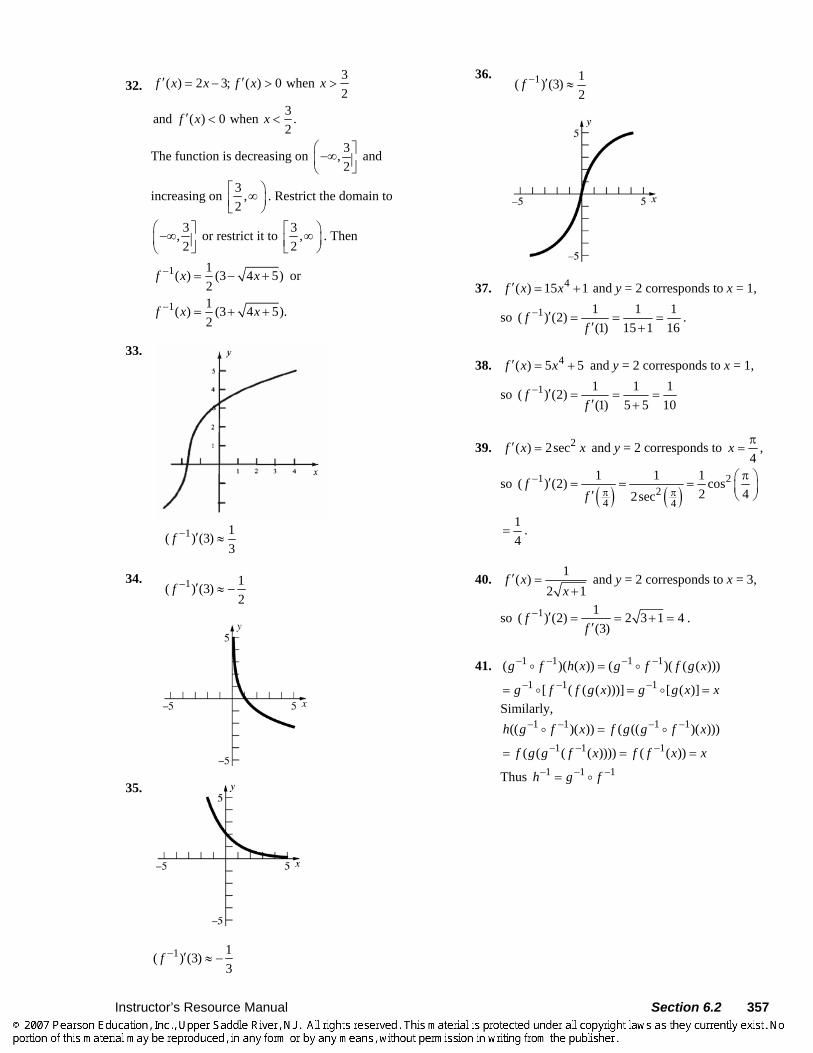
33.
1 1( ) (3)
3f − ′ ≈
34. 1 1( ) (3)2
f − ′ ≈ −
35.
1 1( ) (3)3
f − ′ ≈ −
36. 1 1( ) (3)2
f − ′ ≈
37. 4( ) 15 1f x x′ = + and y = 2 corresponds to x = 1,
so 1 1 1 1( ) (2)(1) 15 1 16
ff
− ′ = = =′ +
.
38. 4( ) 5 5f x x′ = + and y = 2 corresponds to x = 1,
so 1 1 1 1( ) (2)(1) 5 5 10
ff
− ′ = = =′ +
39. 2( ) 2secf x x′ = and y = 2 corresponds to 4
x π= ,
so ( ) ( )
1 22
4 4
1 1 1( ) (2) cos2 42sec
ff
−π π
π⎛ ⎞′ = = = ⎜ ⎟′ ⎝ ⎠
14
= .
40. 1( )2 1
f xx
′ =+
and y = 2 corresponds to x = 3,
so 1 1( ) (2) 2 3 1 4(3)
ff
− ′ = = + =′
.
41. –1 –1 –1 –1( )( ( )) ( )( ( ( )))g f h x g f f g x= –1 –1 –1[ ( ( ( )))] [ ( )]g f f g x g g x x= = =
Similarly, –1 –1 –1 –1(( )( )) ( (( )( )))h g f x f g g f x=
–1 –1 –1( ( ( ( )))) ( ( ))f g g f x f f x x= = =
Thus –1 –1 –1h g f=
358 Section 6.2 Instructor’s Resource Manual
42. Find 1( ) :f x− 1yx
= , 1xy
=
1 1( )f yy
− =
1 1( )f xx
− =
Find 1( ) :g x− y = 3x + 2
23
yx −=
1 2( )3
yg y− −=
1 2( )3
xg x− −=
1( ) ( ( )) (3 2)3 2
h x f g x f xx
= = + =+
( )11 1 1 1 21( ) ( ( ))
3xh x g f x g
x− − − −
−⎛ ⎞= = =⎜ ⎟⎝ ⎠
1 1 1 (3 2) 2 3( ( ))3 2 3 3
x xh h x h xx
− − + −⎛ ⎞= = = =⎜ ⎟+⎝ ⎠
( )( ) ( )
11
11
2 1 1( ( ))3 2 2
x
xx
h h x h x−⎛ ⎞−⎜ ⎟= = = =⎜ ⎟ ⎡ ⎤− +⎝ ⎠ ⎣ ⎦
43. f has an inverse because it is monotonic (increasing):
2( ) 1 cos 0f x x′ = + >
a. ( ) ( )
12
2 2
1 1( ) ( ) 11 cos
f Af
−π π
′ = = =′ +
b. ( ) ( )
15 2 756 46
1 1 1( ) ( )1 cos
f Bf
−π π
′ = = =′ +
27
=
c. 12
1 1 1( ) (0)(0) 21 cos (0)
ff
− ′ = = =′ +
44. a. ax bycx d
+=
+
cxy + dy = ax + b (cy – a)x = b – dy
b dy dy bxcy a cy a
− −= = −
− −
1( ) dy bf ycy a
− −= −
−
1( ) dx bf xcx a
− −= −
−
b. If bc – ad = 0, then f(x) is either a constant function or undefined.
c. If 1f f −= , then for all x in the domain we have:
0ax b dx bcx d cx a
+ −+ =
+ −
(ax + b)(cx – a) + (dx – b)(cx + d) = 0 2 2 2( )acx bc a x ab dcx+ − − +
2( ) 0d bc x bd+ − − = 2 2 2( ) ( ) ( ) 0ac dc x d a x ab bd+ + − + − − =
Setting the coefficients equal to 0 gives three requirements: (1) a = –d or c = 0 (2) a = ±d (3) a = –d or b = 0 If a = d, then 1f f −= requires b = 0 and
c = 0, so ( ) axf x xd
= = . If a = –d, there are
no requirements on b and c (other than 0bc ad− ≠ ). Therefore, 1f f −= if a = –d
or if f is the identity function. 45.
1 10
( )f y dy− =∫ (Area of region B)
= 1 – (Area of region A) 10
2 31 ( ) 15 5
f x dx= − = − =∫
Instructor’s Resource Manual Section 6.3 359
46. 0
( )a
f x dx =∫ the area bounded by y = f(x), y = 0,
and x = a [the area under the curve]. –1
0( )
bf y dy =∫ the area bounded by –1( )x f y=
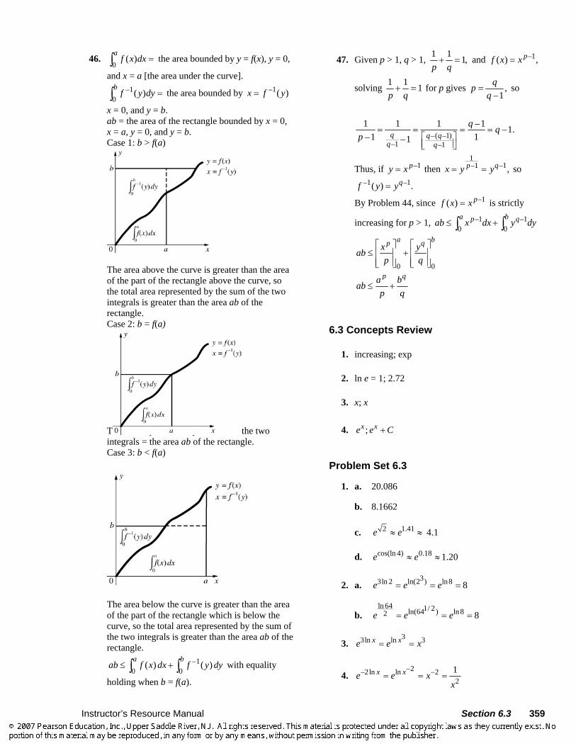
x = 0, and y = b. ab = the area of the rectangle bounded by x = 0, x = a, y = 0, and y = b. Case 1: b > f(a)
The area above the curve is greater than the area of the part of the rectangle above the curve, so the total area represented by the sum of the two integrals is greater than the area ab of the rectangle. Case 2: b = f(a)
The area represented by the sum of the two integrals = the area ab of the rectangle. Case 3: b < f(a)
The area below the curve is greater than the area of the part of the rectangle which is below the curve, so the total area represented by the sum of the two integrals is greater than the area ab of the rectangle.
10 0
( ) ( )a b
ab f x dx f y dy−≤ +∫ ∫ with equality
holding when b = f(a).
47. Given p > 1, q > 1, 1 1 1,p q
+ = and –1( ) ,pf x x=
solving 1 1 1p q
+ = for p gives ,–1qp
q= so
–( –1)
–1 –1
1 1 1 –1 –1.–1 1–1q q q
q q
q qp
= = = =⎡ ⎤⎢ ⎥⎣ ⎦
Thus, if –1py x= then 1
–1–1 ,qpx y y= = so –1 –1( ) .qf y y=
By Problem 44, since 1( ) pf x x −= is strictly
increasing for p > 1, –1 –10 0a bp qab x dx y dy≤ +∫ ∫
0 0
a bp qx yabp q
⎡ ⎤ ⎡ ⎤≤ +⎢ ⎥ ⎢ ⎥
⎢ ⎥ ⎢ ⎥⎣ ⎦ ⎣ ⎦
p qa babp q
≤ +
6.3 Concepts Review
1. increasing; exp
2. ln e = 1; 2.72
3. x; x
4. ; x xe e C+
Problem Set 6.3
1. a. 20.086
b. 8.1662
c. 2 1.41e e≈ ≈ 4.1
d. cos(ln 4) 0.18 1.20e e≈ ≈
2. a. 33ln 2 ln(2 ) ln8 8e e e= = =
b. ln 64 1/ 2ln(64 ) ln82 8e e e= = =
3. 33ln ln 3x xe e x= =
4. 2–2ln ln 2
21x xe e xx
− −= = =
360 Section 6.3 Instructor’s Resource Manual
5. cosln cosxe x=
6. –2 –3ln –2 – 3xe x=
7. 3 –3 3 –3ln( ) ln ln 3ln – 3x xx e x e x x= + =
8. –lnln
x xx x
xe ee
xe= =
9. 2ln 3 2ln ln 3 2 ln ln 23 3x x xe e e e x+ = ⋅ = ⋅ =
10. 2ln 2 22ln – ln 2–
ln ln
xx y x y
y x y yx
e x xe xe xe
= = = =
11. 2 2 2( 2)x x xx xD e e D x e+ + += + =
12. 2 22 – 2 – 2(2 – )x x x x
x xD e e D x x= 22 – (4 –1)x xe x=
13. 2
2 2 22 2
xx x
x xeD e e D x
x
++ += + =
+
14. 1 1– –2 2
2
1–1 2– 2 –33
1–
22
x xx x
xx
D e e Dx
ee xx
⎛ ⎞= ⎜ ⎟
⎝ ⎠
= ⋅ =
15. 22ln lnx x
x xD e D e= 2 2xD x x= =
16. ln ln ln2
1(ln ) 1–
ln (ln )
x x xx x xx x
x xx xD e e D ex x
⋅ ⋅= = ⋅
ln
2(ln –1)
(ln )
xxe x
x=
17. 3 3 3( ) ( )x x xx x xD x e x D e e D x= +
3 2 23 ( 3)x x xx e e x x e x= + ⋅ = +
18. 3 3ln ln 3( ln )x x x x
x xD e e D x x= 3 ln 3 21 ln 3x xe x x x
x⎛ ⎞= ⋅ + ⋅⎜ ⎟⎝ ⎠
3 ln 2 2( 3 ln )x xe x x x= + 32 ln (1 3ln )x xx e x= +
19. 2 2 2 21 2[ ] ( )x x x x
x x xD e e D e D e+ = + 2 2 21 2 21 ( )
2x x x
x xe D e e D x−= +
2 2 21 2 22
1 ( )2
x x xx
xe e D x ex
−= + ⋅
2 21 21 ( ) 22
x x xe x ex
= + ⋅
22 x
x xex ex
= +
20. 2 2 21
21x x x
x x xx
D e D e D ee
− −⎡ ⎤⎢ ⎥+ = +⎢ ⎥⎣ ⎦
2 22 2[ ]x xx xe D x e D x
− − −= + − 2 23( 2 ) ( 2 )x xe x e x
− − −= ⋅ − + ⋅ − 21
3 22 2x
x
e xx e
= − −
21. [ ] [2]xyx xD e xy D+ =
( ) ( ) 0xyx xe xD y y xD y y+ + + =
0xy xyx xxe D y ye xD y y+ + + =
– –xy xyx xxe D y xD y ye y+ =
– ( 1)– –( 1)
xy xy
x xy xyye y y e yD y
xxe x x e− +
= = =+ +
22. [ ] [4 ]x yx xD e D x y+ = + +
(1 ) 1x yx xe D y D y+ + = +
1x y x yx xe e D y D y+ ++ = +
– 1–x y x yx xe D y D y e+ +=
1– –1–1
x y
x x yeD y
e
+
+= =
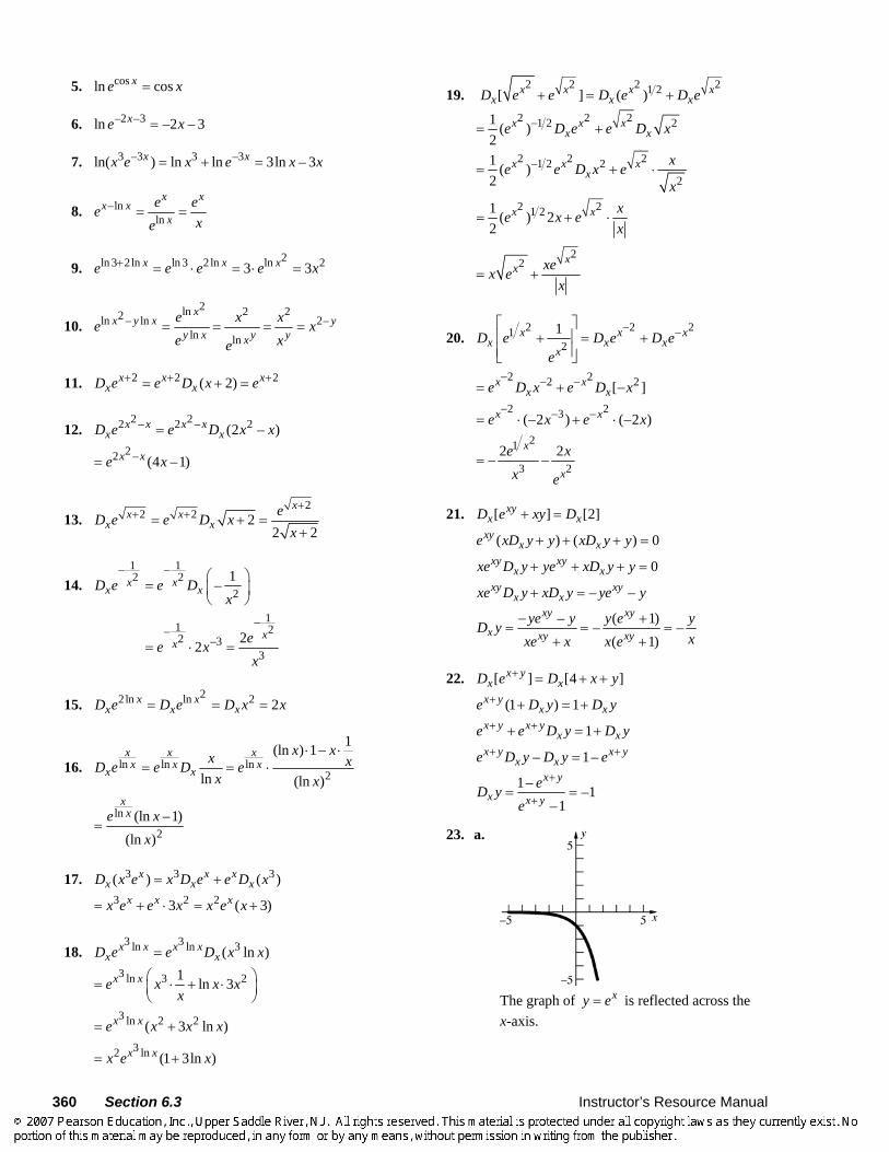
23. a.
The graph of xy e= is reflected across the
x-axis.
Instructor’s Resource Manual Section 6.3 361
b.
The graph of xy e= is reflected across the
y-axis.
24. – –– – ,a ba b a b e e< ⇒ > ⇒ > since xe is an increasing function.
25. 2( ) xf x e= Domain = ( , )−∞ ∞ 2 2( ) 2 , ( ) 4x xf x e f x e′ ′′= =
Since ( ) 0f x′ > for all x, f is increasing on ( , )−∞ ∞ . Since ( ) 0f x′′ > for all x, f is concave upward on ( , )−∞ ∞ . Since and f f ′ are both monotonic, there are no extreme values or points of inflection.
2−2 x
y
4
8
26. 2( )x
f x e−= Domain = ( , )−∞ ∞
2 21 1( ) , ( )2 4
x xf x e f x e− −′ ′′= − =
Since ( ) 0f x′ < for all x, f is decreasing on ( , )−∞ ∞ . Since ( ) 0f x′′ > for all x, f is concave upward on ( , )−∞ ∞ . Since and f f ′ are both monotonic, there are no extreme values or points of inflection.
5−5 x
y
4
8
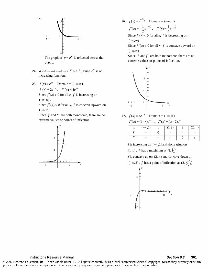
27. ( ) xf x xe−= Domain = ( , )−∞ ∞
( ) (1 ) , ( ) ( 2)x xf x x e f x x e− −′ ′′= − = −
( ,1) 1 (1, 2) 2 (2, )0
0
xff
−∞ ∞′ + − − −′′ − − − +
f is increasing on ( ,1]−∞ and decreasing on
[1, )∞ . f has a maximum at 1(1, )e
f is concave up on (2, )∞ and concave down on
( , 2)−∞ . f has a point of inflection at 22(2, )
e
−3
5
−5
x
y
8
362 Section 6.3 Instructor’s Resource Manual
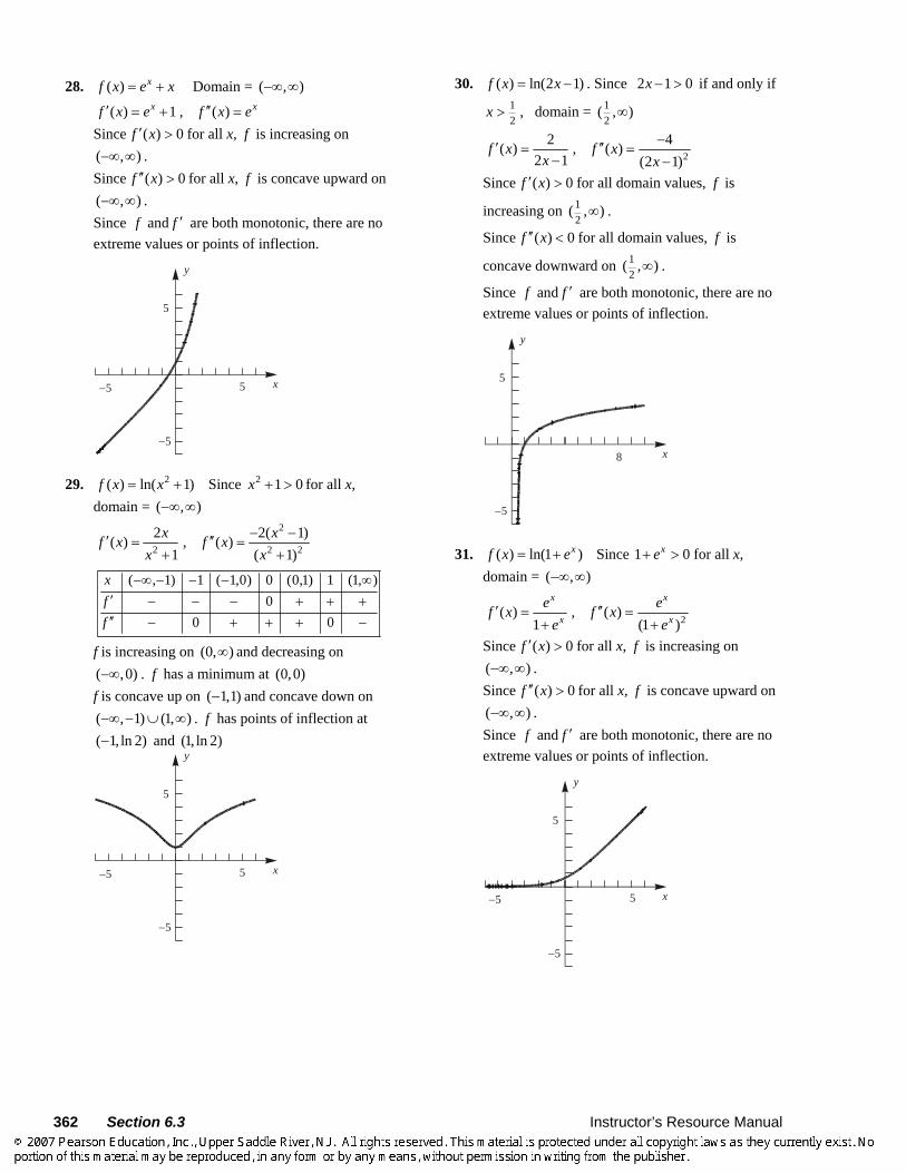
28. ( ) xf x e x= + Domain = ( , )−∞ ∞
( ) 1 , ( )x xf x e f x e′ ′′= + = Since ( ) 0f x′ > for all x, f is increasing on ( , )−∞ ∞ . Since ( ) 0f x′′ > for all x, f is concave upward on ( , )−∞ ∞ . Since and f f ′ are both monotonic, there are no extreme values or points of inflection.
−5 5
5
−5
x
y
29. 2( ) ln( 1)f x x= + Since 2 1 0x + > for all x, domain = ( , )−∞ ∞
2
2 2 22 2( 1)( ) , ( )
1 ( 1)x xf x f x
x x− −′ ′′= =
+ +
( , 1) 1 ( 1,0) 0 (0,1) 1 (1, )0
0 0
xff
−∞ − − − ∞′ − − − + + +′′ − + + + −
f is increasing on (0, )∞ and decreasing on ( ,0)−∞ . f has a minimum at (0,0) f is concave up on ( 1,1)− and concave down on ( , 1) (1, )−∞ − ∪ ∞ . f has points of inflection at ( 1, ln 2)− and (1, ln 2)
−5 5
5
−5
x
y
30. ( ) ln(2 1)f x x= − . Since 2 1 0x − > if and only if 12
x > , domain = 12
( , )∞
22 4( ) , ( )
2 1 (2 1)f x f x
x x−′ ′′= =
− −
Since ( ) 0f x′ > for all domain values, f is
increasing on 12
( , )∞ .
Since ( ) 0f x′′ < for all domain values, f is
concave downward on 12
( , )∞ .
Since and f f ′ are both monotonic, there are no extreme values or points of inflection.
8
5
−5
x
y
31. ( ) ln(1 )xf x e= + Since 1 0xe+ > for all x, domain = ( , )−∞ ∞
2( ) , ( )1 (1 )
x x
x xe ef x f x
e e′ ′′= =
+ +
Since ( ) 0f x′ > for all x, f is increasing on ( , )−∞ ∞ . Since ( ) 0f x′′ > for all x, f is concave upward on ( , )−∞ ∞ . Since and f f ′ are both monotonic, there are no extreme values or points of inflection.
−5 5
5
−5
x
y
Instructor’s Resource Manual Section 6.3 363
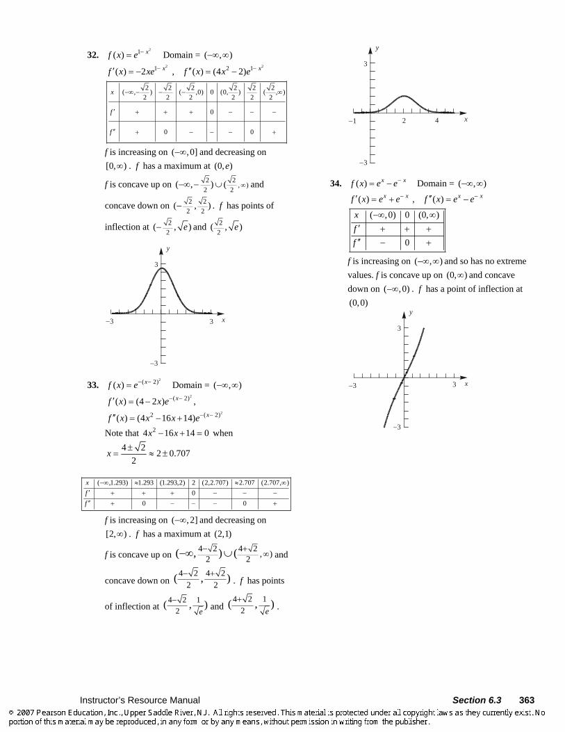
32. 21( ) xf x e −= Domain = ( , )−∞ ∞
2 21 2 1( ) 2 , ( ) (4 2)x xf x xe f x x e− −′ ′′= − = −
2 2 2 2 2 2( , ) ( ,0) 0 (0, ) ( , )2 2 2 2 2 2
0
0 0
x
f
f
−∞ − − − ∞
′ + + + − − −
′′ + − − − +
f is increasing on ( ,0]−∞ and decreasing on [0, )∞ . f has a maximum at (0, )e
f is concave up on 2 2, )
2 2( , ) ( ∞−∞ − ∪ and
concave down on 2 22 2
( , )− . f has points of
inflection at 22
( , )e− and 22
( , )e
−3
x
y
−3 3
3
33. 2( 2)( ) xf x e− −= Domain = ( , )−∞ ∞
2
2
( 2)
2 ( 2)
( ) (4 2 ) ,
( ) (4 16 14)
x
x
f x x e
f x x x e
− −
− −
′ = −
′′ = − +
Note that 24 16 14 0x x− + = when 4 2 2 0.707
2x ±
= ≈ ±
( ,1.293) 1.293 (1.293,2) 2 (2,2.707) 2.707 (2.707, )0
0 0
xff
−∞ ≈ ≈ ∞′ + + + − − −′′ + − − − +
f is increasing on ( , 2]−∞ and decreasing on [2, )∞ . f has a maximum at (2,1)
f is concave up on 4 2 4 2 , )2 2( , ) (− +
∞−∞ ∪ and
concave down on 4 2 4 2
2 2( , )− +
. f has points
of inflection at 4 2 1
2( , )
e−
and 4 2 1
2( , )
e+
.
−1 2 4
−3
x
y
3
34. ( ) x xf x e e−= − Domain = ( , )−∞ ∞
( ) , ( )x x x xf x e e f x e e− −′ ′′= + = −
( ,0) 0 (0, )
0
xff
−∞ ∞′ + + +′′ − +
f is increasing on ( , )−∞ ∞ and so has no extreme values. f is concave up on (0, )∞ and concave down on ( ,0)−∞ . f has a point of inflection at (0,0)
−3 3
−3
x
y
3
364 Section 6.3 Instructor’s Resource Manual
35. 2
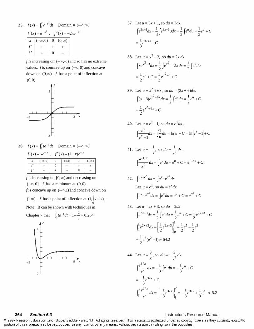
0( ) x tf x e dt−= ∫ Domain = ( , )−∞ ∞ 2 2
( ) , ( ) 2x xf x e f x xe− −′ ′′= = −
( ,0) 0 (0, )
0
xff
−∞ ∞′ + + +′′ + −
f is increasing on ( , )−∞ ∞ and so has no extreme values. f is concave up on ( ,0)−∞ and concave down on (0, )∞ . f has a point of inflection at (0,0)
−3 3
−3
x
y
3
36. 0( ) x tf x te dt−= ∫ Domain = ( , )−∞ ∞
( ) , ( ) (1 )x xf x xe f x x e− −′ ′′= = − ( ,0) 0 (0,1) 1 (1, )
00
xff
−∞ ∞′ − + + +′′ + + + −
f is increasing on [0, )∞ and decreasing on ( ,0]−∞ . f has a minimum at (0,0) f is concave up on ( ,1)−∞ and concave down on
(1, )∞ . f has a point of inflection at 1
0(1, )tte dt−∫ .
Note: It can be shown with techniques in
Chapter 7 that 10
21 0.264tte dte
− = − ≈∫
−2
9
4
−3 x
y
37. Let u = 3x + 1, so du = 3dx. 3 1 3 11 1 13
3 3 3x x u ue dx e dx e du e C+ += = = +∫ ∫ ∫
3 113
xe C+= +
38. Let 2 3,u x= − so du = 2x dx. 2 23 31 12
2 2x x uxe dx e x dx e du− −= =∫ ∫ ∫
2 31 12 2
u xe C e C−= + = +
39. Let 2 6u x x= + , so du = (2x + 6)dx. 2 6 1 1( 3)
2 2x x u ux e dx e du e C++ = = +∫ ∫
2 612
x xe C+= +
40. Let 1, so x xu e du e dx= − = .
1 ln ln 11
xx
xe dx du u C e C
ue= = + = − +
−∫ ∫
41. Let 1 ,ux
= − so 21du dxx
= .
1/1/
2
xu u xe dx e du e C e C
x
−−= = + = +∫ ∫
42. x xx e x ee dx e e dx+ = ⋅∫ ∫
Let , so .x xu e du e dx= = x xx e u u ee e dx e du e C e C⋅ = = + = +∫ ∫
43. Let u = 2x + 3, so du = 2dx 2 3 2 31 1 1
2 2 2x u u xe dx e du e C e C+ += = + = +∫ ∫
11 2 3 2 3 5 30 0
1 1 1–2 2 2
x xe dx e e e+ +⎡ ⎤= =⎢ ⎥⎣ ⎦∫
3 21 ( 1) 64.22
e e= − ≈
44. Let 3ux
= , so 23 .du dxx
= −
3 /
21 1– –3 3
xu ue dx e du e C
x= = +∫ ∫
3/1–3
xe C= +
23 /2 3/ 3 / 2 321 1
1 1 1– –3 3 3
xxe dx e e e
x⎡ ⎤= = +⎢ ⎥⎣ ⎦∫ ≈ 5.2
Instructor’s Resource Manual Section 6.3 365
45. ln 3 ln 32 20 0
( )x xV e dx e dx= π = π∫ ∫
ln 32 2ln 3 0
0
1 1 1 4 12.572 2 2
xe e e π⎡ ⎤ ⎛ ⎞= π = π − = ≈⎜ ⎟⎢ ⎥⎣ ⎦ ⎝ ⎠
46. 21
02 xV xe dx−= π∫ .
Let 2u x= − , so du = –2x dx. 2 2
2 ( 2 )x x uxe dx e x dx e du− −π = −π − = −π∫ ∫ ∫ 2u xe C e C−= −π + = −π +
12 21 1 00 0
2 – ( )x xxe dx e e e− − −⎡ ⎤π = −π = π −⎢ ⎥⎣ ⎦∫
1(1 )e−= π − 1.99≈
47. The line through (0, 1) and 11, e
⎛ ⎞⎜ ⎟⎝ ⎠
has slope
1 1 1 1 11 1 ( 0);1 0e e ey x
e e e
− − −= − = ⇒ − = −
−
1 1ey xe−
= +
11 20 0
1 112
x xe ex e dx x x ee e
− −⎡ − ⎤ −⎛ ⎞ ⎡ ⎤+ − = + +⎜ ⎟⎢ ⎥ ⎢ ⎥⎝ ⎠ ⎣ ⎦⎣ ⎦∫
1 1 31 1 0.0522 2
e ee e e
− −= + + − = ≈
48. –2 –
( –1)(1) – ( ) 1( ) – (– )(–1)( –1) 1–
x xx
x xe x ef x e
e e′ =
21 1 1
( 1) 1
x x
x x xe xe
e e e−− − ⎛ ⎞
= − ⎜ ⎟− − ⎝ ⎠
21 1
( 1) 1
x x
x xe xe
e e− −
= −− − 2
1 ( 1)( 1)
x x x
xe xe e
e− − − −
=−
2( 1)
x
xxe
e= −
−
When x > 0, ( ) 0,f x′ < so f(x) is decreasing for x > 0.
49. a. Exact: 10! 10 9 8 7 6 5 4 3 2 1
3,628,800= ⋅ ⋅ ⋅ ⋅ ⋅ ⋅ ⋅ ⋅ ⋅=
Approximate: 101010! 20 3,598,696
e⎛ ⎞≈ π ≈⎜ ⎟⎝ ⎠
b. 60
816060! 120 8.31 10e
⎛ ⎞≈ π ≈ ×⎜ ⎟⎝ ⎠
50. ( )0.3 0.3 0.3 0.31 1 1 0.3 14 3 2
e⎧ ⎫⎡ ⎤⎛ ⎞≈ + + + +⎨ ⎬⎜ ⎟⎢ ⎥⎝ ⎠⎣ ⎦⎩ ⎭
1.3498375= 0.3 1.3498588e ≈ by direct calculation
51. sin ,tx e t= so ( sin cos )t tdx e t e t dt= +
cos ,ty e t= so ( cos sin )t tdy e t e t dt= − 2 2
2 2(sin cos ) (cos sin )t
ds dx dy
e t t t t dt
= +
= + + −
2 22sin 2cos 2t te t tdt e dt= + = The length of the curve is
0 0
2 2 2( 1) 31.312t te dt e eππ π⎡ ⎤= = − ≈⎣ ⎦∫
52. Use x = 30, n = 8, and k = 0.25. 8 0.25 30( ) (0.25 30)( )
! 8!
n kx
nkx e eP x
n
− − ⋅⋅= = 0.14≈
53. a. 20
lnlim is of the form 1 (ln )x
xx+→
∞∞+
.
1
2 10 0
lnlim lim
2ln[1 (ln ) ]x x
x xx x
D xxD x+ +→ →
= =⋅+
0
1lim 02lnx x+→
= =
2ln 1lim lim 0
2ln1 (ln )x x
xxx→∞ →∞
= =+
b. 2 1 1
2 2
[1 (ln ) ] – ln 2ln( )
[1 (ln ) ]x xx x x
f xx
+ ⋅ ⋅ ⋅′ =
+
2
2 21– (ln )
[1 (ln ) ]x
x x=
+
1( ) 0 when ln 1 so f x x x e e′ = = ± = =
–1 1 or x ee
= =
2 2ln 1 1( )
21 (ln ) 1 1ef ee
= = =+ +
( )1
2 21
ln1 –1 1–21 (–1)1 ln
e
e
fe
⎛ ⎞ = = =⎜ ⎟⎝ ⎠ ++
Maximum value of 12
at x = e; minimum
value of 12
− at 1.x e−=
366 Section 6.3 Instructor’s Resource Manual
c. 2
21ln( )
1 (ln )
x tF x dtt
=+∫
2
2 2ln( ) 2
1 (ln )xF x xx
′ = ⋅+
2
2 2 2ln( ) 1( ) 2 2
1 [ln( ) ] 1 1eF e e ee
′ = ⋅ = ⋅+ +
1.65e= ≈
54. Let 00( , )xx e be the point of tangency. Then 0
0 0 00 0 00
– 0 ( ) 1– 0
xx x xe f x e e x e x
x′= = ⇒ = ⇒ =
so the line is 0xy e x= or y = ex.
a. 121
00
( – ) –2
x x exA e ex dx e⎡ ⎤
= = ⎢ ⎥⎢ ⎥⎣ ⎦
∫
= 0( 0) –1 0.362 2e ee e− − − = ≈
b. 1 2 20[( ) – ( ) ]xV e ex dx= π∫
1 2 2 20
( – )xe e x dx= π∫ 12 3
2
0
1 –2 3
x e xe⎡ ⎤
= π ⎢ ⎥⎢ ⎥⎣ ⎦
22 01 1
2 3 2ee e
⎡ ⎤⎛ ⎞= π − −⎢ ⎥⎜ ⎟⎝ ⎠⎢ ⎥⎣ ⎦
2( – 3) 2.306
eπ= ≈
55. a. 3 3
2 23 01 1exp 2 exp 3.11dx dxx x−
⎛ ⎞ ⎛ ⎞− = − ≈⎜ ⎟ ⎜ ⎟
⎝ ⎠ ⎝ ⎠∫ ∫
b. 8 0.10
sinxe x dxπ −∫ ≈ 0.910
56. a. 10
lim (1 ) xx
x e→
+ = ≈ 2.72
b. 10
1lim (1 ) xx
xe
−
→+ = ≈ 0.368
57. 2
( ) xf x e−= 2
( ) 2 xf x xe−′ = − 2 2 22 2( ) 2 4 2 (2 1)x x xf x e x e e x− − −′′ = − + = −
y = f(x) and ( )y f x′′= intersect when 2 2 2 22 (2 1); 1 4 2;x xe e x x− −= − = −
2 34 3 0, 2
x x− = = ±
Both graphs are symmetric with respect to the
y-axis so the area is 3 2 2 22
0
2 23 23
2
2 [ 2 (2 1)]
[2 (2 1) ]
x x
x x
e e x dx
e x e dx
−
− −
⎧⎪ − −⎨⎪⎩
⎫⎪+ − − ⎬⎪⎭
∫
∫
≈ 4.2614
58. a. –lim 0p xx
x e→∞
=
b. – – –1( ) (–1)p x x pf x x e e px′ = + ⋅ –1 – ( – )p xx e p x=
( ) 0f x′ = when x = p
59. 2 ––
lim ln( )xx
x e→ ∞
+ = ∞ (behaves like x− )
2 –lim ln( )xx
x e→∞
+ = ∞ (behaves like 2ln x )
60. –1 –1–2 –2( ) –(1 ) (– )x xf x e e x′ = + ⋅
1/
2 1/ 2(1 )
x
xe
x e=
+
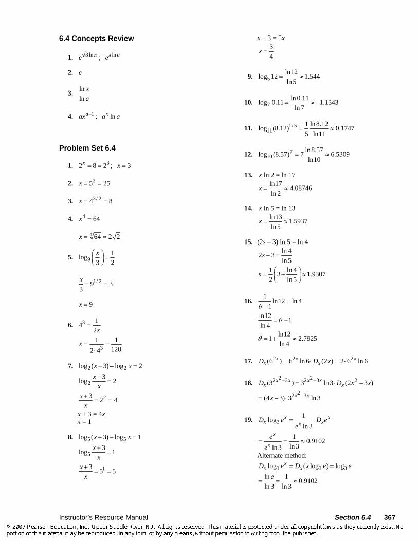
a. 0
lim ( ) 0x
f x+→
=
b. –0
lim ( ) 1x
f x→
=
c. 1lim ( )2x
f x→±∞
=
d. 0
lim ( ) 0x
f x→
′ =
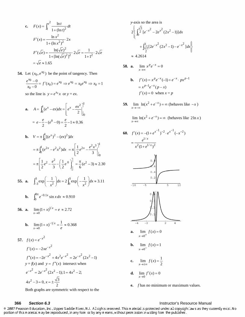
e. f has no minimum or maximum values.
Instructor’s Resource Manual Section 6.4 367
6.4 Concepts Review
1. 3 lne π ; lnx ae
2. e
3. lnln
xa
4. 1aax − ; lnxa a
Problem Set 6.4
1. 32 8 2x = = ; 3x =
2. 25 25x = =
3. 3/ 24 8x = =
4. 4 64x =
4 64 2 2x = =
5. 91log
3 2x⎛ ⎞ =⎜ ⎟
⎝ ⎠
1/ 29 33x
= =
9x =
6. 3 142x
=
31 1
1282 4x = =
⋅
7. 2 2log ( 3) – log 2x x+ =
23log 2x
x+
=
23 2 4xx+
= =
x + 3 = 4x x = 1
8. 5 5log ( 3) – log 1x x+ =
53log 1x
x+
=
13 5 5xx+
= =
x + 3 = 5x 34
x =
9. 5ln12log 12 1.544ln 5
= ≈
10. 7ln 0.11log 0.11 –1.1343
ln 7= ≈
11. 1/ 511
1 ln8.12log (8.12) 0.17475 ln11
= ≈
12. 710
ln8.57log (8.57) 7 6.5309ln10
= ≈
13. x ln 2 = ln 17 ln17 4.08746ln 2
x = ≈
14. x ln 5 = ln 13 ln13 1.5937ln 5
x = ≈
15. (2s – 3) ln 5 = ln 4 ln 42 – 3ln 5
s =
1 ln 43 1.93072 ln 5
s ⎛ ⎞= + ≈⎜ ⎟⎝ ⎠
16. 1 ln12 ln 4–1θ
=
ln12 –1ln 4
θ=
ln121 2.7925ln 4
θ = + ≈
17. 2 2 2(6 ) 6 ln 6 (2 ) 2 6 ln 6x x xx xD D x= ⋅ = ⋅
18. 2 22 –3 2 –3 2(3 ) 3 ln 3 (2 – 3 )x x x x
x xD D x x= ⋅ 22 –3(4 – 3) 3 ln 3x xx= ⋅
19. 31logln 3
x xx xxD e D e
e= ⋅
1 0.9102ln 3ln 3
x
xe
e= = ≈
Alternate method:
3 3 3log ( log ) logxx xD e D x e e= = ln 1 0.9102ln 3 ln 3
e= = ≈
368 Section 6.4 Instructor’s Resource Manual
20. 3 310 3
1log ( 9) ( 9)( 9) ln10
x xD x D xx
+ = ⋅ ++
2
33
( 9) ln10x
x=
+
21. [3 ln( 5)]13 (1) ln( 5) 3 ln 3
5
zz
z z
D z
zz
+
= ⋅ + + ⋅+
13 ln( 5) ln 35
z zz
⎡ ⎤= + +⎢ ⎥+⎣ ⎦
22. 2 – 2
10 10log (3 ) ( – ) log 3D Dθ θθ θ θ θ=
22( – ) ln 3 ln 3 –
ln10 ln10D Dθ θ
θ θ θ θ= = ⋅
2 –1/ 2ln 3 1 ( – ) (2 –1)ln10 2
θ θ θ= ⋅
2
2 –1 ln 3ln102 –
θ
θ θ=
23. Let 2u x= so du = 2xdx. 2 1 1 22 2
2 2 ln 2
ux ux dx du C⋅ = = ⋅ +∫ ∫
2 2 –12 2 2 ln 2 ln 2
x xC C= + = +
24. Let u = 5x – 1, so du = 5 dx.
5 –1 1 1 1010 105 5 ln10
ux udx du C= = ⋅ +∫ ∫
5 –1105ln10
xC= +
25. Let 1, so .2
u x du dxx
= =
5 52 5 2ln 5
x uudx du C
x= = ⋅ +∫ ∫
2 5ln 5
xC⋅
= +
44
11
5 5 25 52 2ln 5 ln 5 ln 5
x xdx
x
⎡ ⎤ ⎛ ⎞⎢ ⎥= = −⎜ ⎟⎢ ⎥ ⎝ ⎠⎣ ⎦∫
40 24.85ln 5
= ≈
26. 1 1 13 –3 3 –30 0 0
(10 10 ) 10 10x x x xdx dx dx+ = +∫ ∫ ∫
Let u = 3x, so du = 3dx.
3 1 1 1010 103 3 ln10
ux udx du C= = ⋅ +∫ ∫
3103ln10
xC= +
Now let u = –3x, so du = –3dx.
–3 1 1 1010 – 10 –3 3 ln10
ux udx du C= = ⋅ +∫ ∫
–310–3ln10
xC= +
Thus, 13 –31 3 –3
00
10 –10(10 10 )3ln10
x xx x dx
⎡ ⎤+ = ⎢ ⎥
⎢ ⎥⎣ ⎦∫
1 1 999,9991000 –3ln10 1000 3000ln10
⎛ ⎞= =⎜ ⎟⎝ ⎠
≈ 144.76
27. 2 2 2( ) ( ) 2 ( )10 10 ln10 10 2 ln10x x xd d x x
dx dx= =
2 10 20 19( ) 20d dx x xdx dx
= =
2( ) 2 10[10 ( ) ]xdy d xdx dx
= +
2( ) 1910 2 ln10 20x x x= +
28. 2sin 2sin sin 2sin cosd dx x x x xdx dx
= =
sin sin sin2 2 ln 2 sin 2 ln 2cosx x xd d x xdx dx
= =
2 sin(sin 2 )xdy d xdx dx
= +
sin2sin cos 2 cos ln 2xx x x= +
29. 1 ( 1)d x xdx
π+ π= π +
( 1) ( 1) ln( 1)x xddx
π + = π + π +
1[ ( 1) ]xdy d xdx dx
π+= + π +
( 1) ( 1) ln( 1)xxπ= π + + π + π +
Instructor’s Resource Manual Section 6.4 369
30. ( ) ( ) ( )2 2 ln 2 2 ln 2x x xe e x e xd d e e
dx dx= =
(2 ) (2 ) ln 2 (2 ) ln 2e x e x e e xd edx
= =
( )[2 (2 ) ]xe e xdy d
dx dx= +
( )2 ln 2 (2 ) ln 2xe x e xe e= +
31. 22 ln (ln ) ln( 1)( 1) x x xy x e += + =
2(ln ) ln( 1) 2[(ln ) ln( 1)]x xdy de x xdx dx
+= +
2(ln ) ln( 1) 22
1 2ln( 1) ln1
x x xe x xx x
+ ⎡ ⎤= + +⎢ ⎥
+⎣ ⎦
22 ln
2ln( 1) 2 ln( 1)
1x x x xx
x x
⎛ ⎞+= + +⎜ ⎟⎜ ⎟+⎝ ⎠
32. 22 2 3 (2 3) ln(ln )(ln ) x x xy x e+ += =
2(2 3) ln(ln ) 2[(2 3) ln(ln )]x xdy de x xdx dx
+= +
2(2 3) ln(ln ) 22 2
1 12ln(ln ) (2 3) (2 )ln
x xe x x xx x
+ ⎡ ⎤= + +⎢ ⎥
⎣ ⎦
2 3
2 2ln ln
2 3(2 ln ) 2 ln (2ln )ln
x
x x
xx xx x
+⎡ ⎤
+⎢ ⎥= +⎢ ⎥⎢ ⎥⎣ ⎦
33. sin sin ln( ) x x xf x x e= =
sin ln( ) (sin ln )x x df x e x xdx
′ =
sin ln 1(sin ) (cos )(ln )x xe x x xx
⎡ ⎤⎛ ⎞= +⎜ ⎟⎢ ⎥⎝ ⎠⎣ ⎦
sin sin cos lnx xx x xx
⎛ ⎞= +⎜ ⎟⎝ ⎠
sin1 sin1(1) 1 cos1ln1 sin1 0.84151
f ⎛ ⎞′ = + = ≈⎜ ⎟⎝ ⎠
34. ( ) 22.46ef e = π ≈
( ) 23.14g e eπ= ≈ g(e) is larger than f(e).
( ) lnx xdf xdx
′ = π = π π
( ) ln 25.71ef e′ = π π ≈
1( ) dg x x xdx
π π−′ = = π
1( ) 26.74g e eπ−′ = π ≈ ( )g e′ is larger than ( )f e′ .
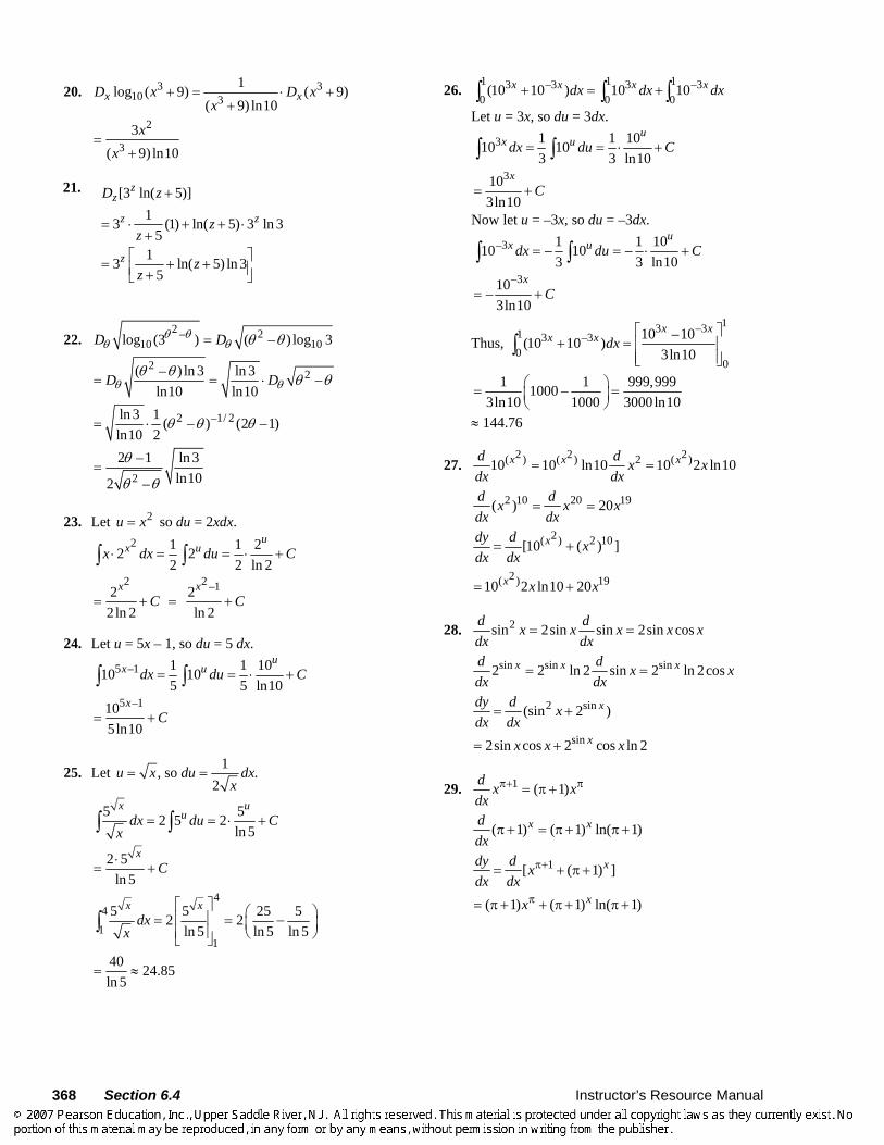
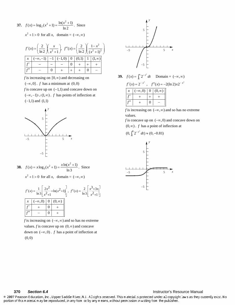
35. (ln 2)( )( ) 2 x xf x e− −= = Domain = ( , )−∞ ∞ 2( ) ( ln 2)2 , ( ) (ln 2) 2x xf x f x− −′ ′′= − =
Since ( ) 0f x′ < for all x, f is decreasing on ( , )−∞ ∞ . Since ( ) 0f x′′ > for all x, f is concave upward on ( , )−∞ ∞ . Since and f f ′ are both monotonic, there are no extreme values or points of inflection.
−2
9
4
−3 x
y
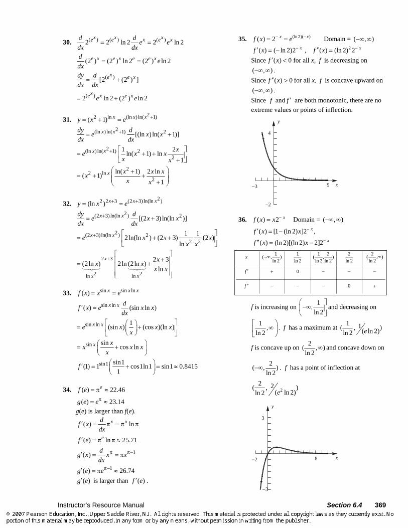
36. ( ) 2 xf x x −= Domain = ( , )−∞ ∞
( ) [1 (ln 2) ]2 ,
( ) (ln 2)[(ln 2) 2]2
x
x
f x x
f x x
−
−
′ = −
′′ = −
1 1 1 2 2 2( , ) ( , ) ( , )ln 2 ln 2 ln 2 ln 2 ln 2 ln 2
0
0
x
f
f
−∞ ∞
′ + − − −
′′ − − − +
f is increasing on ,1
ln 2⎛ ⎤
−∞⎜ ⎥⎝ ⎦
and decreasing on
1 ,ln 2
⎡ ⎞∞⎟⎢
⎣ ⎠. f has a maximum at 1 1( , )( ln 2)ln 2 e
f is concave up on 2( , )ln 2
∞ and concave down on
2( , )ln 2
−∞ . f has a point of inflection at
22 2( , )
( ln 2)ln 2 e
8
−3
3
−2 x
y
370 Section 6.4 Instructor’s Resource Manual
37. 2
22
ln( 1)( ) log ( 1)ln 2xf x x +
= + = . Since
2 1 0x + > for all x, domain = ( , )−∞ ∞
2
2 2 22 2 1( ) , ( )
ln 2 ln 21 ( 1)x xf x f x
x x⎛ ⎞⎛ ⎞ ⎛ ⎞ −⎛ ⎞′ ′′= = ⎜ ⎟⎜ ⎟ ⎜ ⎟⎜ ⎟ ⎜ ⎟+ +⎝ ⎠⎝ ⎠ ⎝ ⎠⎝ ⎠
( , 1) 1 ( 1,0) 0 (0,1) 1 (1, )0
0 0
xff
−∞ − − − ∞′ − − − + + +′′ − + + + −
f is increasing on [0, )∞ and decreasing on ( ,0]−∞ . f has a minimum at (0,0) f is concave up on ( 1,1)− and concave down on ( , 1) (1, )−∞ − ∪ ∞ . f has points of inflection at ( 1,1)− and (1,1)
−5
5
5
−5
x
y
38. 2
23
ln( 1)( ) log ( 1)ln 3
x xf x x x += + = . Since
2 1 0x + > for all x, domain = ( , )−∞ ∞
2 31 22 32( ) ln( 1) , ( )2 2ln 3 ln31 1
x x xf x x f xx x
⎡ ⎤ ⎡ ⎤+′ ′′⎢ ⎥ ⎢ ⎥= + + =⎢ ⎥ ⎢ ⎥+ +⎣ ⎦ ⎣ ⎦
( ,0) 0 (0, )00
xff
−∞ ∞′ + +′′ − +
f is increasing on ( , )−∞ ∞ and so has no extreme values. f is concave up on (0, )∞ and concave down on ( ,0)−∞ . f has a point of inflection at (0,0)
−5
5
5
−5
x
y
39. 2
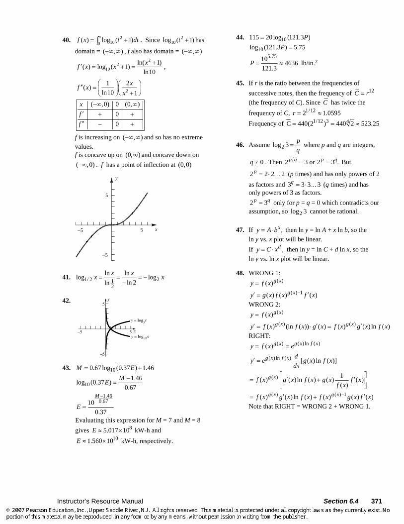
1( ) 2x tf x dt−= ∫ Domain = ( , )−∞ ∞ 2 2
( ) 2 , ( ) 2(ln 2) 2x xf x f x x− −′ ′′= = −
( ,0) 0 (0, )
0
xff
−∞ ∞′ + + +′′ + −
f is increasing on ( , )−∞ ∞ and so has no extreme values. f is concave up on ( ,0)−∞ and concave down on (0, )∞ . f has a point of inflection at
201(0, 2 ) (0, 0.81)t dt− ≈ −∫
−5
5
5
−5
x
y
Instructor’s Resource Manual Section 6.4 371
40. 2100( ) log ( 1)xf x t dt= +∫ . Since 2
10log ( 1)t + has
domain = ( , )−∞ ∞ , f also has domain = ( , )−∞ ∞2
210
2
ln( 1)( ) log ( 1) ,ln10
1 2( )ln10 1
xf x x
xf xx
+′ = + =
⎛ ⎞⎛ ⎞′′ = ⎜ ⎟⎜ ⎟+⎝ ⎠⎝ ⎠
( ,0) 0 (0, )00
xff
−∞ ∞′ + +′′ − +
f is increasing on ( , )−∞ ∞ and so has no extreme values. f is concave up on (0, )∞ and concave down on ( ,0)−∞ . f has a point of inflection at (0,0)
−5
5
5
−5
x
y
41. 1/ 2 212
ln lnlog logln 2ln
x xx x= = = −−
42.
43. 100.67 log (0.37 ) 1.46M E= +
101.46log (0.37 )
0.67ME −
=
1.460.6710
0.37
M
E
−
=
Evaluating this expression for M = 7 and M = 8 gives 85.017 10E ≈ × kW-h and
101.560 10E ≈ × kW-h, respectively.
44. 10115 20log (121.3 )P=
10log (121.3 ) 5.75P = 5.7510 4636
121.3P = ≈ lb/in.2
45. If r is the ratio between the frequencies of successive notes, then the frequency of 12C r= (the frequency of C). Since C has twice the frequency of C, 1/122 1.0595r = ≈ Frequency of 1/12 3 4C 440(2 ) 440 2 523.25= = ≈
46. Assume 2log 3 pq
= where p and q are integers,
0q ≠ . Then 2 3 or 2 3 .p q p q= = But
2 2 2 2p = ⋅ … (p times) and has only powers of 2 as factors and 3 3 3 3q = ⋅ … (q times) and has only powers of 3 as factors. 2 3p q= only for p = q = 0 which contradicts our assumption, so 2log 3 cannot be rational.
47. If ,xy A b= ⋅ then ln y = ln A + x ln b, so the ln y vs. x plot will be linear. If ,dy C x= ⋅ then ln y = ln C + d ln x, so the ln y vs. ln x plot will be linear.
48. WRONG 1: ( )( )g xy f x=
( ) 1( ) ( ) ( )g xy g x f x f x−′ ′= WRONG 2:
( )( )g xy f x= ( ) ( )( ) (ln ( )) ( ) ( ) ( ) ln ( )g x g xy f x f x g x f x g x f x′ ′ ′= ⋅ =
RIGHT: ( ) ( ) ln ( )( )g x g x f xy f x e= =
( ) ln ( ) [ ( ) ln ( )]g x f x dy e g x f xdx
′ =
( ) 1( ) ( ) ln ( ) ( ) ( )( )
g xf x g x f x g x f xf x
⎡ ⎤′ ′= +⎢ ⎥⎣ ⎦
( ) ( ) 1( ) ( ) ln ( ) ( ) ( ) ( )g x g xf x g x f x f x g x f x−′ ′= + Note that RIGHT = WRONG 2 + WRONG 1.
372 Section 6.4 Instructor’s Resource Manual
49. 2( ) ( )( ) ( ) ( )
xx x x xf x x x x g x= = ≠ = 2 2( ) ln( ) x x xf x x e= = 2 ln 2
2 ln 2
2( )
( ) ( ln )
12 ln
(2 ln )
x x
x x
x
df x e x xdx
e x x xx
x x x x
′ =
⎛ ⎞= + ⋅⎜ ⎟⎝ ⎠
= +
( ) ln( )x xx x xg x x e= =
Using the result from Example 5
(1 ln ) :x xd x x xdx
⎛ ⎞= +⎜ ⎟⎝ ⎠
ln( ) ( ln )xx x xdg x e x x
dx′ =
ln 1(1 ln ) lnxx x x xe x x x x
x⎡ ⎤= + + ⋅⎢ ⎥⎣ ⎦
( ) 1(1 ln ) lnxx xx x x x
x⎡ ⎤= + +⎢ ⎥⎣ ⎦
2 1ln (ln )xx xx x x
x+ ⎡ ⎤= + +⎢ ⎥⎣ ⎦
50. 1( )1
x
xaf xa
−=
+
2 2( 1) ln ( 1) ln 2 ln( )
( 1) ( 1)
x x x x x
x xa a a a a a a af x
a a+ − −′ = =
+ +
Since a is positive, xa is always positive. 2( 1)xa + is also always positive, thus ( ) 0f x′ >
if ln a > 0 and ( ) 0f x′ < if ln a < 0. f(x) is either always increasing or always decreasing, depending on a, so f(x) has an inverse.
11
x
xaya
−=
+
( 1) 1x xy a a+ = −
( 1) 1xa y y− = − − 11
x yay
+=
−
1ln ln1
yx ay
+=
−
11ln 1log
ln 1
yy
ayx
a y
+− +
= =−
1 1( ) log1a
yf yy
− +=
−
1 1( ) log1a
xf xx
− +=
−
51. a. Let g(x) = ln f(x) = ln ln lna
xx a x x aa
⎛ ⎞= −⎜ ⎟⎜ ⎟
⎝ ⎠.
( ) lnag x ax
⎛ ⎞′ = −⎜ ⎟⎝ ⎠
( ) 0 when ,lnag x xa
′ < > so as x → ∞ g(x)
is decreasing. 2( ) ag xx
′′ = − , so g(x) is
concave down. Thus, lim ( ) ,x
g x→∞
= −∞ so
( )lim ( ) lim 0.g xx x
f x e→∞ →∞
= =
b. Again let g(x) = ln f(x) = a ln x – x ln a. Since y = ln x is an increasing function, f(x) is maximized when g(x) is maximized.
( ) ln , so ( ) 0 on 0, ln
a ag x a g xx a
⎛ ⎞ ⎛ ⎞′ ′= − >⎜ ⎟ ⎜ ⎟⎝ ⎠ ⎝ ⎠
and ( ) 0 on , .lnag xa
⎛ ⎞′ < ∞⎜ ⎟⎝ ⎠
Therefore, g(x) (and hence f(x)) is
maximized at 0 .lnaxa
=
c. Note that a xx a= is equivalent to g(x) = 0.
By part b., g(x) is maximized at 0 .lnaxa
=
If a = e, then
0( ) ( ) ln ln 0.lneg x g g e e e e ee
⎛ ⎞= = = − =⎜ ⎟⎝ ⎠
Since 0( ) ( ) 0g x g x< = for all 0 ,x x≠ the
equation g(x) = 0 (and hence a xx a= ) has just one positive solution. If a e≠ , then
0( ) ln (ln )ln ln lna a ag x g a aa a a
⎛ ⎞ ⎛ ⎞= = −⎜ ⎟ ⎜ ⎟⎝ ⎠ ⎝ ⎠
ln 1lnaaa
⎡ ⎤⎛ ⎞= −⎜ ⎟⎢ ⎥⎝ ⎠⎣ ⎦.
Now lna ea
> (justified below), so
0( ) ln 1 (ln 1) 0.lnag x a a ea
⎡ ⎤= − > − =⎢ ⎥⎣ ⎦ Since
0 0( ) 0 on (0, ), ( ) 0, and g x x g x′ > >
0lim ( ) ,x
g x→
= −∞ g(x) = 0 has exactly one
solution on 0(0, ).x Since 0( ) 0 on ( , )g x x′ < ∞ ,
0( ) 0, and lim ( ) ,x
g x g x→∞
> = −∞ g(x) = 0 has
exactly one solution on 0( , ).x ∞ Therefore,
Instructor’s Resource Manual Section 6.4 373
the equation g(x) = 0 (and hence a xx a= ) has exactly two positive solutions.
To show that lna ea
> when a e≠ :
Consider the function ( ) , for 1.ln
xh x xx
= >
( )1
2 2
ln( )(1) ln 1( )(ln ) (ln )
xx x xh xx x
− −′ = =
Note that ( ) 0h x′ < on (1, e) and ( ) 0h x′ > on (e, ∞ ), so h(x) has its minimum at (e, e).
Therefore ln
x ex
> for all x e≠ , x > 1.
d. For the case a = e, part c. shows that ( ) ln ln 0g x e x x e= − < for x e≠ .
Therefore, when x e≠ , ln ln ,e xx e< which
implies .e xx e< In particular, .e eππ <
52. a. ( ) u xuf x x e−=
1 1( ) ( )u x u x u xuf x ux e x e u x x e− − − − −′ = − = −
Since ( ) 0uf x′ > on (0, u) and ( ) 0uf x′ < on (u, ∞ ), ( )uf x attains its maximum at x0 = u.
b. ( ) ( 1)u uf u f u> + means ( 1)( 1)u u u uu e u e− − +> + .
Multiplying by 1u
ueu
+ gives 1 uue
u+⎛ ⎞> ⎜ ⎟
⎝ ⎠.
1 1( 1) ( ) means u uf u f u+ ++ > 1 ( 1) 1( 1)u u u uu e u e+ − + + −+ > .
Multiplying by 1
1
u
ueu
+
+ gives
11 uu eu
++⎛ ⎞ >⎜ ⎟⎝ ⎠
.
Combining the two inequalities, 11 1u uu ue
u u
++ +⎛ ⎞ ⎛ ⎞< <⎜ ⎟ ⎜ ⎟⎝ ⎠ ⎝ ⎠
.
c. From part b., 11 uue
u
++⎛ ⎞< ⎜ ⎟⎝ ⎠
.
Multiplying by 1
uu +
gives
11
uu ueu u
+⎛ ⎞< ⎜ ⎟+ ⎝ ⎠.
We showed 1 uu eu+⎛ ⎞ <⎜ ⎟
⎝ ⎠ in part b., so
11
uu ue eu u
+⎛ ⎞< <⎜ ⎟+ ⎝ ⎠.
Since lim1u
u e eu→∞
=+
, this implies that
1 1lim , i.e., lim 1u u
u u
u e eu u→∞ →∞
+⎛ ⎞ ⎛ ⎞= + =⎜ ⎟ ⎜ ⎟⎝ ⎠ ⎝ ⎠
.
53. ln( ) x x xf x x e= = Let ( ) ln .g x x x= Using L’Hôpital’s Rule,
10 0
1
10 02
lnlim ( ) lim
lim lim ( ) 0
x x x
x
x xx
xg x
x
+ +→ →
+ +→ →
=
= = − =−
Therefore, 0
0lim 1x
xx e
+→= = .
( ) 1 lng x x′ = + Since ( ) 0g x′ < on ( )0,1/ e and ( ) 0g x′ > on
( )1/ ,e ∞ , g(x) has its minimum at 1ex = .
Therefore, f(x) has its minimum at 1 1/( , )ee e− − . Note: this point could also be written as
( )1
11 ,e
ee
⎛ ⎞⎜ ⎟⎜ ⎟⎝ ⎠
.
54.
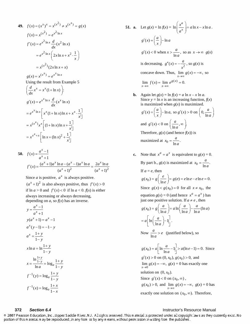
(2.4781, 15.2171), (3, 27)
55. 4 sin0
20.2259xx dxπ
≈∫
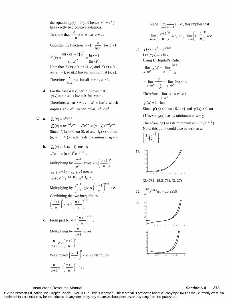
56.
374 Section 6.5 Instructor’s Resource Manual
57. a. In order of increasing slope, the graphs represent the curves 2 , 3 ,x xy y= = and
4 .xy =
b. ln y is linear with respect to x, and at x = 0, y = 1 since C = 1.
c. The graph passes through the points (0.2, 4) and (0.6, 8). Thus, 0.24 Cb= and 0.68 .Cb= Dividing the second equation by the first, gets 0.4 5 22 so 2 .b b= = Therefore 3 22 .C =
58. The graph of the equation whose log-log plot has negative slope contains the points (2, 7) and (7, 2).
Thus, 7 2 and 2 7 ,r rC C= = so 7 2 .2 7
r⎛ ⎞= ⎜ ⎟⎝ ⎠
7 2 ln 7 ln 2ln ln 12 7 ln 2 ln 7
r r −= ⇒ = = −
− and C = 14.
Hence, one equation is 114 .y x−= The graph of one equation contains the points (7, 30) and (10, 70). Thus, 30 7rC= and
70 10 ,rC= so 3 77 10
r⎛ ⎞= ⎜ ⎟⎝ ⎠
3 7 ln 3 ln 7ln ln 2.387 10 ln 7 ln10
r r −= ⇒ = ≈
− and
2.3830 7 0.29C −≈ ⋅ ≈ . Hence, another equation is 2.380.29 .y x=
The graph of another equation contains the points (1, 2) and (7, 5). Thus, 2 1rC= and 5 7 ,rC= so C = 2 and
ln 5 ln 2 ln 7r− =ln 5 ln 2 0.47.
ln 7r −
⇒ = ≈
Hence, the last equation is 0.472y x= . The given answers are only approximate. Student answers may also vary.
6.5 Concepts Review
1. ;ky ( )ky L y− 2. 32 8=
3. half-life 4. ( )1/1 hh+
Problem Set 6.5
1. 6k = − , 60 4, so 4 ty y e−= =
2. 606, 1, so tk y y e= = =
3. 0.00500.005, so tk y y e= =
0.005(10) 0.050 0(10)y y e y e= =
0 0.052(10) 2y y
e= ⇒ =
0.005 0.005 0.05 0.005( 10)0.052 2 2t t ty e e e
e− −= = =
4. k = –0.003, so –0.0030
ty y e= (–0.003)(–2) 0.006
0 0(–2)y y e y e= =
0 0.0063( 2) 3y y
e− = ⇒ =
–0.003 –0.003 –0.006 –0.003( 2)0.0063 3 3t t ty e e e
e+= = =
5. 0 10,000,y = y(10) = 20,000 (10)20,000 10,000 ke=
102 ke=
ln 2 = 10k; ln 210
k =
((ln 2) /10) /1010,000 10,000 2t ty e= = ⋅
After 25 days, 2.510,000 2 56,568.y = ⋅ ≈
6. Since the growth is exponential and it doubles in 10 days (from t = 0 to t = 10), it will always double in 10 days.
7. ((ln 2) /10)0 03 ty y e=
((ln 2) /10)3 te= ln 2ln 310
t=
10 ln 3 15.8ln 2
t = ≈ days
Instructor’s Resource Manual Section 6.5 375
8. Let P(t) = population (in millions) in year 1790 + t. In 1960, t = 170.
0( ) ktP t P e= 170178 3.9 ke=
17045.64 ke= ln 45.64 0.02248
170k = ≈
In 2000, t = 210 0.02248 210(210) 3.9 438P e ⋅≈ ≈
The model predicts that the population will be about 438 million. The actual number, 275 million, is quite a bit smaller because the rate of growth has declined in recent decades.
9. 1 year: (4.5 million) (1.032) 4.64≈ million
2 years: (4.5 million) 2(1.032) 4.79≈ million
10 years: (4.5 million) 10(1.032) 6.17≈ million
100 years: (4.5 million) 100(1.032) 105≈ million
10. 0kty y e=
(1)1.032 kA Ae= ln1.032 0.03150k = ≈
At t = 100, (0.03150)(100)4.5 105y e= ≈ . After 100 years, the population will be about 105 million.
11. The formula to use is 0kty y e= , where y =
population after t years, 0y =population at time t = 0, and k is the rate of growth. We are given
(12)0
(5)0
235,000 and
164,000
k
k
y e
y e
=
=
Dividing one equation by the other yields 12 5 71.43293 k k ke e−= = or
ln(1.43293) 0.05138887
k = ≈
Thus 0 12(0.0513888)235,000 126,839.y
e= =
12. The formula to use is 0kty y e= , where y = mass t
months after initial measurement, 0y = mass at time of initial measurement, and k is the rate of growth. We are given
(4)6.76 4 ke= so that 1 6.76 0.5247ln 0.13124 4 4
k ⎛ ⎞= = ≈⎜ ⎟⎝ ⎠
Thus, 6 months before the initial measurement, the mass was (0.1312)( 6)4 1.82y e −= ≈ grams. The tumor would have been detectable at that time.
13. (700)0
1 and 102
ke y= =
–ln 2 = 700k ln 2 0.00099700
k = − ≈ −
0.0009910 ty e−=
At t = 300, 0.00099 30010 7.43.y e− ⋅= ≈ After 300 years there will be about 7.43 g.
14. (2)0.85 ke= ln 0.85 = 2k
ln 0.85 0.08132
k = ≈ −
0.081312
te−=
– ln 2 0.0813t= − ln 2 8.53
0.0813t = ≈
The half-life is about 8.53 days.
15. The basic formula is 0kty y e= . If *t denotes the
half-life of the material, then (see Example 3)
*12
kte= or *
ln(0.5)kt
= . Thus
0.693 0.6930.0229 and 0.024130.22 28.8C Sk k− −
= = − = = −
To find when 1% of each material will remain, we
use 0 0ln(0.01)0.01 or kty y e t
k= = . Thus
4.6052 201 years (2187)0.02294.6052 191 years (2177)0.0241
C
S
t
t
−= ≈
−−
= ≈−
and
16. The basic formula is 0kty y e= . We are given
(2) (8)0 015.231 and 9.086k ky e y e= =
Dividing one equation by the other gives
(2) (8) ( 6)15.2319.086
k k ke e− −= = so 0.0861k = −
Thus 0 ( .0861)(2)15.231 18.093y
e −= ≈ grams.
To find the half-life:
*ln(0.5) 0.693 8
0.0861t
k−
= = ≈−
days
376 Section 6.5 Instructor’s Resource Manual
17. 573012
ke=
( )12 4ln
1.210 105730
k −= ≈ − ×
4( 1.210 10 )0 00.7 ty y e
−− ×=
4ln 0.7 2950
1.210 10t
−= ≈
− ×
The fort burned down about 2950 years ago.
18. 573012
ke=
( )12 4ln
1.210 105730
k −= ≈ − ×
4( 1.210 10 )0 00.51 ty y e
−− ×=
4ln 0.51 5565
1.210 10t
−= ≈
− ×
The body was buried about 5565 years ago.
19. From Example 4, 1 0 1( ) ( ) ktT t T T T e= + − . In this
problem, (0.5)200 (0.5) 75 (300 75) kT e= = + − so125ln225 1.1756
0.5k
⎛ ⎞⎜ ⎟⎝ ⎠= = − and
( 1.1756)(3)(3) 75 225 81.6 FT e −= + =
20. From Example 4, 1 0 1( ) ( ) ktT t T T T e= + − . In this
problem, (5)0 (5) 24 ( 20 24) kT e= = + − − so24ln44 0.1212
5k
−⎛ ⎞⎜ ⎟−⎝ ⎠= = − ; the thermometer will
register 20 C when 0.121220 24 ( 44) te−= + − or 4ln
44 19.780.1212
t
−⎛ ⎞⎜ ⎟−⎝ ⎠= =
−min.
21. From Example 4, 1 0 1( ) ( ) ktT t T T T e= + − . In this
problem, (5)70 (5) 90 (26 90) kT e= = + − so20ln64 0.2326
5k
−⎛ ⎞⎜ ⎟−⎝ ⎠= = − and
( 0.2326)(10)(10) 90 64 90 64(0.0977) 83.7 CT e −= − = − =
22. From Example 4, 1 0 1( ) ( ) ktT t T T T e= + − . In this
problem, (15)250 (15) 40 (350 40) kT e= = + − so210ln310 0.02615
k
⎛ ⎞⎜ ⎟⎝ ⎠= = − ; the brownies will be
110 F when 0.026110 40 (310) te−= + or 70ln
310 57.20.026
t
⎛ ⎞⎜ ⎟⎝ ⎠= =
−min.
23. From Example 4, 1 0 1( ) ( ) ktT t T T T e= + − . Let w = the time of death; then
(10 )
(11 )
82 (10 ) 70 (98.6 70)
76 (11 ) 70 (98.6 70)
k w
k w
T w e
T w e
−
−
= − = + −
= − = + −
or (10 )
(11 )
12 28.6
6 28.6
k w
k w
e
e
−
−
=
=
Dividing: ( 1)2 or ln (0.5) 0.693ke k−= = = −
To find w :
0.693(10 )
12ln28.612 28.6 so 10 1.25
0.693we w− −
⎛ ⎞⎜ ⎟⎝ ⎠= − = =
−Therefore 10 1.25 8.75 8 : 45pmw = − = = .
24. a. From example 4 of this section,
1( )dT k T Tdt
= − or
11
or ln T(t)-TdT k dt kt CT T
= = +−∫
This gives 1( ) kt CT t T e e− = . Now, if 0T is
the temperature at t = 0, 0 1CT T e− = and the
Law of Cooling becomes
1 0 1( ) ktT t T T T e− = − . Note that ( )T t is always between 0T and 1T so that
1 0 1( ) and T t T T T− − always have the same sign; this simplifies the Law of Cooling to
1 0 1( ) ( ) ktT t T T T e− = − or
1 0 1( ) ( ) ktT t T T T e= + −
b. Since ( )T t is always between 0T and 1T , it
follows that 1
0 1
( )1kt T t T
eT T
−= <
− so that 0k < .
Hence
1 0 1 1 1lim ( ) ( ) lim 0kt
t tT t T T T e T T
→∞ →∞= + − = + =
Instructor’s Resource Manual Section 6.5 377
25. a. 2($375)(1.035) $401.71≈
b. 240.035($375) 1 $402.15
12⎛ ⎞+ ≈⎜ ⎟⎝ ⎠
c. 7300.035($375) 1 $402.19
365⎛ ⎞+ ≈⎜ ⎟⎝ ⎠
d. 0.035 2($375) $402.19e ⋅ ≈
26. a. 2($375)(1.046) $410.29=
b. 240.046($375) 1 $411.06
12⎛ ⎞+ ≈⎜ ⎟⎝ ⎠
c. 7300.046($375) 1 $411.13
365⎛ ⎞+ ≈⎜ ⎟⎝ ⎠
d. 0.046 2($375) $411.14e ⋅ ≈
27. a. 120.061 2
12
t⎛ ⎞+ =⎜ ⎟⎝ ⎠
121.005 2t = ln 212
ln1.005t = so ln 2 11.58
12ln1.005t = ≈
It will take about 11.58 years or 11 years, 6 months, 29 days.
b. 0.06 2te = ⇒ln 2 11.550.06
t = ≈
It will take about 11.55 years or 11 years, 6 months, and 18 days.
28. 5$20,000(1.025) $22,628.16≈
29. 1626 to 2000 is 374 years. 0.06 37424 $133.6y e ⋅= ≈ billion
30. 969 18$100(1.04) $3.201 10≈ ×
31. (0.05)(1)1000 $1051.27e =
32. (0.05)(1)0 1000A e =
0.050 1000 $951.23A e−= ≈
33. If t is the doubling time, then
1 2100
tp⎛ ⎞+ =⎜ ⎟⎝ ⎠
ln 1 ln 2100
pt ⎛ ⎞+ =⎜ ⎟⎝ ⎠
( ) 100100
ln 2 ln 2 100ln 2 70
ln 1 ppt
p p= ≈ = ≈
+
34. ( – )dy ky L ydt
=
1( – )
dy kdty L y
=
1 1( – )
dy kdtLy L L y
⎡ ⎤+ =⎢ ⎥
⎣ ⎦
1 1 1–
dy kdtL y L y
⎛ ⎞+ =⎜ ⎟
⎝ ⎠∫ ∫
11 [ln – ln ]y L y kt CL
− = +
1ln–y Lkt LC
L y= +
1 1 , so –
Lkt LC LC Lkt Lkty ye e e CeL y L y
+= = ⋅ =−
0 0
0
0
Note that: (0) .
– (0) –
LkC Ce Ceyy
L y L y
⋅⎛ ⎞= =⎜ ⎟⎜ ⎟= =⎜ ⎟⎝ ⎠
–Lkt Lkty LCe yCe= Lkt Lkty yCe LCe+ =
1 –1
Lkt
Lkt LktLkte
LCe LC LCyCCe C e
= = =++ +
0– 0 0
––0 0 0– 0( – )
yL y
y LktLktL y
L Lyy L y ee
⋅= =
++
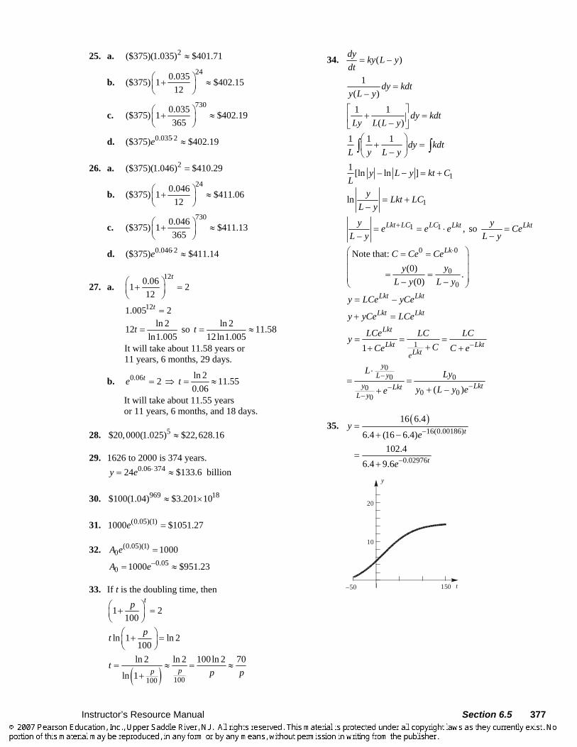
35. ( )
16(0.00186)
0.02976
16 6.4
6.4 (16 6.4)102.4
6.4 9.6
t
t
ye
e
−
−
=+ −
=+
20
t
y
10
−50 150
378 Section 6.5 Instructor’s Resource Manual
36. a. 1000 10000
lim (1 ) 1 1x
x→
+ = =
b. 1/0 0
lim 1 lim 1 1xx x→ →
= =
c. 1/
0lim (1 ) lim (1 )x n
nxε ε
+ →∞→+ = + = ∞
d. 1/
0
1lim (1 ) lim 0(1 )
xnnx
εε− →∞→
+ = =+
e. 1/0
lim (1 ) xx
x e→
+ =
37. a. 1/1 ( )0 0
1 1lim (1 ) lim[1 ( )]
xxx x
xex −→ →
− = =+ −
b. 31
1/ 330 0
lim (1 3 ) lim (1 3 )x xx x
x x e→ →
⎡ ⎤+ = + =⎢ ⎥
⎢ ⎥⎣ ⎦
c. 2 2lim lim 1n n
n n
nn n→∞ →∞
+⎛ ⎞ ⎛ ⎞= +⎜ ⎟ ⎜ ⎟⎝ ⎠ ⎝ ⎠
1/
0lim (1 2 ) x
xx
+→= +
2122
0lim (1 2 ) x
xx e
+→
⎡ ⎤= + =⎢ ⎥
⎢ ⎥⎣ ⎦
d. 2 21 1lim lim 1
n n
n n
nn n→∞ →∞
−⎛ ⎞ ⎛ ⎞= −⎜ ⎟ ⎜ ⎟⎝ ⎠ ⎝ ⎠
2 /
0lim (1 ) x
xx
+→= −
21
20
1lim (1 ) x
xx
e
−−
+→
⎡ ⎤= − =⎢ ⎥
⎢ ⎥⎣ ⎦
38. dy ay bdt
= +
ba
dy a dty
=+∫ ∫
ln by at Ca
+ = +
; at C atb by e y Aea a
++ = + =
at by Aea
= −
0 0b by A A ya a
= − ⇒ = +
0atb by y e
a a⎛ ⎞= + −⎜ ⎟⎝ ⎠
39. Let y = population in millions, t = 0 in 1985, a = 0.012, b = 0.06 , 0 10y =
0.012 0.06dy ydt
= +
0.012 0.0120.06 0.0610 – 15 – 50.012 0.012
t ty e e⎛ ⎞= + =⎜ ⎟⎝ ⎠
From 1985 to 2010 is 25 years. At t = 25, 0.012 2515 5 15.25.y e ⋅= − ≈ The population in 2010
will be about 15.25 million.
40. Let N(t) be the number of people who have heard
the news after t days. Then ( )dN k L Ndt
= − .
1 dN k dtL N
=−∫ ∫
–ln(L – N) = kt + C kt CL N e− −− =
ktN L Ae−= − N(0) = 0, ⇒ A = L
( ) (1 )ktN t L e−= − .
(5)2LN = ⇒ 5(1 )
2kL L e−= −
512
ke−=
12ln
0.13865
k = ≈−
0.1386( ) (1 )tN t L e−= − 0.13860.99 (1 )tL L e−= −
0.13860.01 te−= ln 0.01 330.1386
t = ≈−
99% of the people will have heard about the scandal after 33 days.
41. If f(t) = ,kte then ( )
( )
kt
ktf t ke kf t e
′= = .
42. –1–1 1 0( ) n n
n nf x a x a x a x a= + + ⋅⋅ ⋅ + + ( )lim( )x
f xf x→∞
′
–1 –2–1 1
–1 1 0
( –1)lim
n nn n
nx n n
na x n a x aa x a x a x a→∞
+ + ⋅⋅⋅ +=
+ + ⋅⋅ ⋅ + +( –1) –1 1
2
–1 01–1
lim 0
na n a an nx nx x
a aanx n x n nx xa→∞
+ + ⋅⋅⋅ += =
+ + ⋅⋅ ⋅ + +
Instructor’s Resource Manual Section 6.5 379
43. ( ) 0( )
f x kf x′
= > can be written as
1 dy ky dx
= where y = f(x).
dy k dxy
= has the solution .kxy Ce=
Thus, the equation ( ) kxf x Ce= represents exponential growth since k > 0.
44. ( ) 0( )
f x kf x′
= < can be written as 1 dy ky dx
= where
y = f(x). dy k dxy
= has the solution .kxy Ce=
Thus, ( ) kxf x Ce= which represents exponential decay since k < 0.
45. Maximum population: 2
2 12
10
640 acres 1 person13,500,000 mi acre1 mi
1.728 10 people
⋅ ⋅
= ×
Let t = 0 be in 2004. 9 0.0132 10(6.4 10 ) 1.728 10te× = ×
10
91.728 10ln
6.4 1075.2 years
0.0132t
⎛ ⎞⋅⎜ ⎟⎜ ⎟⋅⎝ ⎠= ≈ from 2004, or
sometime in the year 2079.
46. a. 0.0132 0.0002k t= −
b. ( )' 0.0132 0.0002y t y= −
c. ( )0.0132 0.0002dy t ydt
= −
( )0.0132 0.0002dy t dty
= −
20ln 0.0132 0.0001y t t C= − +
20.0132 0.0001
1t ty C e −=
The initial condition (0) 6.4y = implies that
1 6.4C = . Thus 20.0132 0.00016.4 t ty e −=
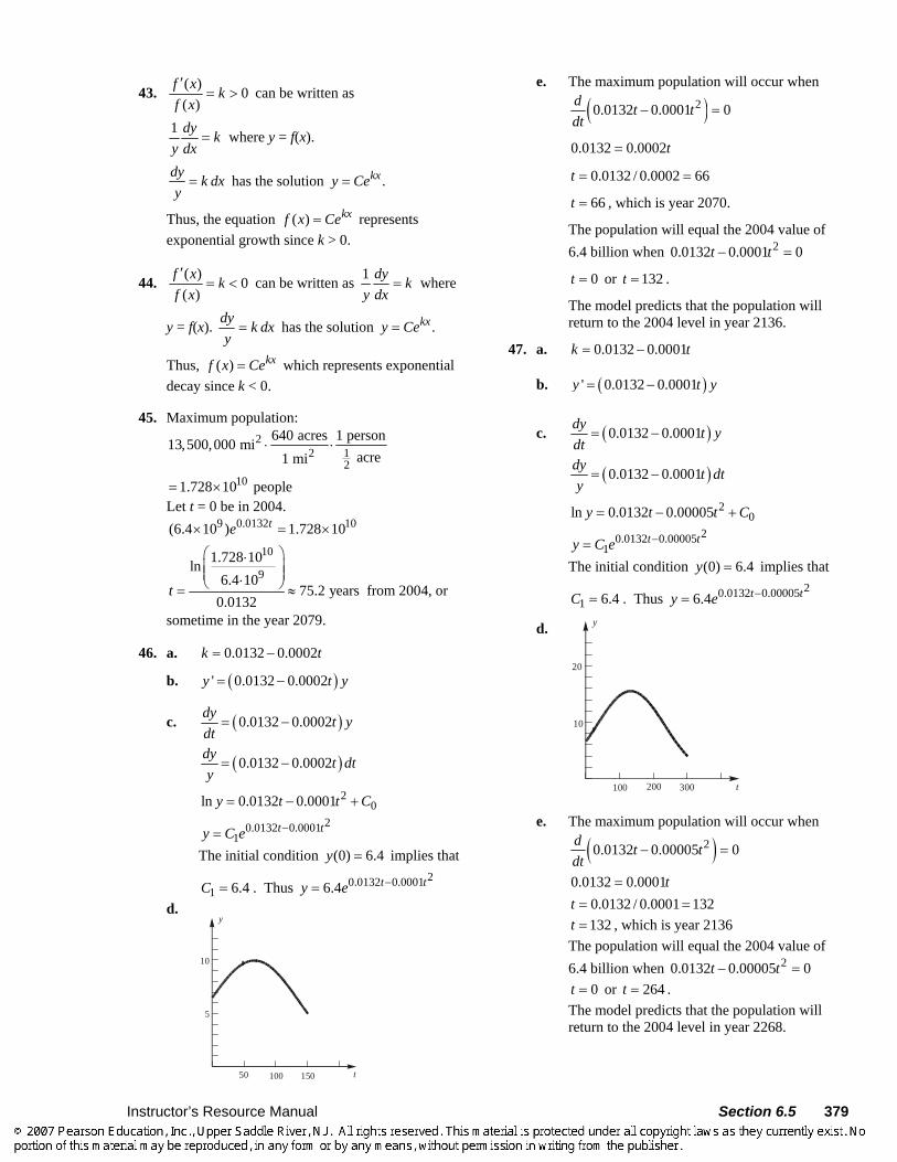
d.
5
t
y
10
50 100 150
e. The maximum population will occur when
( )20.0132 0.0001 0d t tdt
− =
0.0132 0.0002t=
0.0132 / 0.0002 66t = =
66t = , which is year 2070.
The population will equal the 2004 value of 6.4 billion when 20.0132 0.0001 0t t− =
0t = or 132t = .
The model predicts that the population will return to the 2004 level in year 2136.
47. a. 0.0132 0.0001k t= −
b. ( )' 0.0132 0.0001y t y= −
c. ( )0.0132 0.0001dy t ydt
= −
( )0.0132 0.0001dy t dty
= −
20ln 0.0132 0.00005y t t C= − +
20.0132 0.00005
1t ty C e −=
The initial condition (0) 6.4y = implies that
1 6.4C = . Thus 20.0132 0.000056.4 t ty e −=
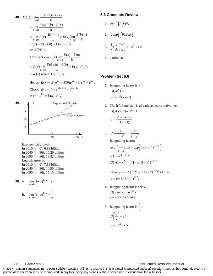
d.
20
t
y
10
300100 200 e. The maximum population will occur when
( )20.0132 0.00005 0d t tdt
− =
0.0132 0.0001t= 0.0132 / 0.0001 132t = = 132t = , which is year 2136 The population will equal the 2004 value of
6.4 billion when 20.0132 0.00005 0t t− = 0t = or 264t = . The model predicts that the population will
return to the 2004 level in year 2268.
380 Section 6.6 Instructor’s Resource Manual
48. 0
( ) – ( )( ) limh
E x h E xE xh→
+′ =
0
( ) ( ) – ( )limh
E x E h E xh→
=
0 0
( ) –1 ( ) –1lim ( ) ( ) limh h
E h E hE x E xh h→ →
= ⋅ =
( ) ( 0) ( ) (0)E x E x E x E= + = ⋅ so (0) 1.E =
Thus, 0
( ) – (0)( ) ( ) limh
E h EE x E xh→
′ =
0
(0 ) – (0)( ) lim ( ) (0)h
E h EE x E x Eh→
+ ′= = ⋅
= kE(x) where (0)k E′= .
Hence, 0( ) (0) 1kx kx kx kxE x E e E e e e= = = ⋅ = .
Check: ( )( ) k u v ku kvE u v e e+ ++ = =
( ) ( )ku kve e E u E v= ⋅ = ⋅
49.
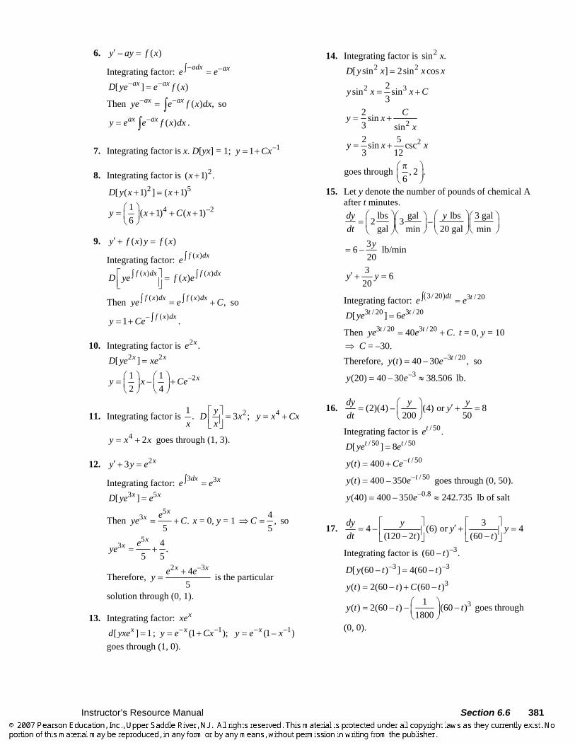
Exponential growth: In 2010 (t = 6): 6.93 billion In 2040 (t = 36): 10.29 billion In 2090 (t = 86): 19.92 billion Logistic growth: In 2010 (t = 6): 7.13 billion In 2040 (t = 36): 10.90 billion In 2090 (t = 86): 15.15 billion
50. a. 1/0
lim (1 ) xx
x e→
+ =
b. 1/0
1lim (1– ) xx
xe→
=
6.6 Concepts Review
1. ( )exp ( )P x dx∫
2. ( )exp ( )y P x dx∫
3. 21 ; 1; d y x Cxx dx x
⎛ ⎞ = +⎜ ⎟⎝ ⎠
4. particular
Problem Set 6.6
1. Integrating factor is xe . ( ) 1xD ye =
– ( )xy e x C= +
2. The left-hand side is already an exact derivative. 2[ ( 1)] –1D y x x+ =
3 – 33( 1)
x x Cyx
+=
+
3. 2 21– 1–x axy yx x
′ + =
Integrating factor: 2 –1/ 2
2exp exp ln(1– )1–
x dx xx
⎡ ⎤= ⎣ ⎦∫
2 –1/ 2(1– )x= 2 –1/ 2 2 –3/ 2[ (1– ) ] (1– )D y x ax x=
Then 2 –1/ 2 2 –1/ 2(1– ) (1– ) ,y x a x C= + so 2 1/ 2(1– ) .y a C x= +
4. Integrating factor is sec x. 2[ sec ] secD y x x=
y = sin x + C cos x
5. Integrating factor is 1 .x
xyD ex
⎡ ⎤ =⎢ ⎥⎣ ⎦
xy xe Cx= +
Instructor’s Resource Manual Section 6.6 381
6. – ( )y ay f x′ =
Integrating factor: – –adx axe e∫ = – –[ ] ( )ax axD ye e f x=
Then – – ( ) ,ax axye e f x dx= ∫ so – ( )ax axy e e f x dx= ∫ .
7. Integrating factor is x. D[yx] = 1; –11y Cx= +
8. Integrating factor is 2( 1) .x + 2 5[ ( 1) ] ( 1)D y x x+ = +
4 –21 ( 1) ( 1)6
y x C x⎛ ⎞= + + +⎜ ⎟⎝ ⎠
9. ( ) ( )y f x y f x′ + =
Integrating factor: ( )f x dxe∫ ( ) ( )( )f x dx f x dxD ye f x e⎡ ⎤∫ ∫=⎢ ⎥⎣ ⎦
Then ( ) ( ) ,f x dx f x dxye e C∫ ∫= + so – ( )1 f x dxy Ce ∫= + .
10. Integrating factor is 2 .xe 2 2[ ]x xD ye xe=
–21 1–2 4
xy x Ce⎛ ⎞ ⎛ ⎞= +⎜ ⎟ ⎜ ⎟⎝ ⎠ ⎝ ⎠
11. Integrating factor is 1 .x
23 ;yD xx
⎡ ⎤ =⎢ ⎥⎣ ⎦ 4y x Cx= +
4 2y x x= + goes through (1, 3).
12. 23 xy y e′ + =
Integrating factor: 3 3dx xe e∫ = 3 5[ ]x xD ye e=
Then 5
3 .5
xx eye C= + x = 0, y = 1 4 ,
5C⇒ = so
53 4 .
5 5
xx eye = +
Therefore, 2 –34
5
x xe ey += is the particular
solution through (0, 1).
13. Integrating factor: xxe [ ] 1xd yxe = ; – –1(1 );xy e Cx= + – –1(1– )xy e x=
goes through (1, 0).
14. Integrating factor is 2sin .x 2 2[ sin ] 2sin cosD y x x x=
2 32sin sin3
y x x C= +
22 sin3 sin
Cy xx
= +
22 5sin csc3 12
y x x= +
goes through , 2 .6π⎛ ⎞
⎜ ⎟⎝ ⎠
15. Let y denote the number of pounds of chemical A after t minutes.
lbs gal lbs 3 gal2 3 –gal min 20 gal min
dy ydt
⎛ ⎞ ⎛ ⎞⎛ ⎞ ⎛ ⎞= ⎜ ⎟ ⎜ ⎟⎜ ⎟ ⎜ ⎟⎝ ⎠ ⎝ ⎠⎝ ⎠ ⎝ ⎠
36 –20
y= lb/min
3 620
y y′ + =
Integrating factor: ( )3/ 20 3 / 20dt te e∫ = 3 / 20 3 / 20[ ] 6t tD ye e=
Then 3 / 20 3 / 2040 .t tye e C= + t = 0, y = 10 ⇒ C = –30. Therefore, –3 / 20( ) 40 – 30 ,ty t e= so
–3(20) 40 – 30 38.506y e= ≈ lb.
16. (2)(4) – (4) or 8200 50
dy y yydt
⎛ ⎞ ′= + =⎜ ⎟⎝ ⎠
Integrating factor is / 50.te / 50 / 50[ ] 8t tD ye e=
– / 50( ) 400 ty t Ce= + – / 50( ) 400 – 350 ty t e= goes through (0, 50).
–0.8(40) 400 – 350 242.735y e= ≈ lb of salt
17. 34 – (6) or 4(120 – 2 ) (60 – )
dy y y ydt t t
⎡ ⎤ ⎡ ⎤′= + =⎢ ⎥ ⎢ ⎥⎣ ⎦ ⎣ ⎦
Integrating factor is –3(60 – ) .t –3 –3[ (60 – ) ] 4(60 – )D y t t=
3( ) 2(60 – ) (60 – )y t t C t= +
31( ) 2(60 – ) – (60 )1800
y t t t⎛ ⎞= −⎜ ⎟⎝ ⎠
goes through
(0, 0).
382 Section 6.6 Instructor’s Resource Manual
18. –250
dy ydt t
=+
or 2 0.50
y yt
′ + =+
Integrating factor: 2 ln(50 ) 22exp (50 )
50tdt e t
t+⎛ ⎞ = = +⎜ ⎟+⎝ ⎠∫
2[ (50 ) ] 0D y t+ =
Then 2(50 ) .y t C+ = t = 0, y = 30 ⇒ C = 75000
Thus, 2(50 ) 75,000.y t+ =
If y = 25, 225(50 ) 75,000,t+ = so
3000 – 50 4.772t = ≈ min.
19. 610 1I I′ + = Integrating factor = 6exp(10 )t
6 6[ exp(10 )] exp(10 )D I t t= –6 6( ) 10 exp(–10 )I t C t= + –6 6( ) 10 [1– exp(–10 )]I t t= goes through (0, 0).
20. 3.5 120sin 377I t′ =
240 sin 3777
I t⎛ ⎞′ = ⎜ ⎟⎝ ⎠
240– cos3772639
I t C⎛ ⎞= +⎜ ⎟⎝ ⎠
240( ) (1– cos377 )2639
I t t⎛ ⎞= ⎜ ⎟⎝ ⎠
through (0, 0).
21. 1000 I = 120 sin 377t I(t) = 0.12 sin 377t
22. 2–100
dx xdt
=
1 050
x x⎛ ⎞′ + =⎜ ⎟⎝ ⎠
Integrating factor is / 50.te / 50[ ] 0tD xe = – / 50tx Ce=
– / 50( ) 50 tx t e= satisfies t = 0, x = 50. – / 50502 – 2
100 200
tdy e ydt
⎛ ⎞ ⎛ ⎞= ⎜ ⎟ ⎜ ⎟⎜ ⎟ ⎝ ⎠⎝ ⎠
– / 501100
ty y e⎛ ⎞′ + =⎜ ⎟⎝ ⎠
Integrating factor is /100.te /100 – /100[ ]t tD ye e=
– /100 – /100( ) ( –100 )t ty t e C e= – /100 – /100( ) (250 –100 )t ty t e e= satisfies t = 0,
y = 150.
23. Let y be the number of gallons of pure alcohol in the tank at time t.
a. 55(0.25) – 1.25 – 0.05100
dyy y ydt
⎛ ⎞′ = = =⎜ ⎟⎝ ⎠
Integrating factor is 0.05te . –0.05( ) 25 ; 100, 0, 75ty t Ce y t C= + = = = –0.05( ) 25 75 ;ty t e= + y = 50, t = T,
T = 20(ln 3) ≈ 21.97 min
b. Let A be the number of gallons of pure alcohol drained away.
(100 – A) + 0.25A = 50 2003
A⇒ =
It took 200
35
minutes for the draining and the
same amount of time to refill, so
( )20032 80 26.67
5 3T = = ≈ min.
c. c would need to satisfy
200 200
3 3 20(ln 3).5 c
+ <
10 7.7170(3ln 3 – 2)
c > ≈
d. 4(0.25) – 0.05 1– 0.05y y y′ = = Solving for y, as in part a, yields
–0.0520 80 .ty e= + The drain is closed when 0.8 .t T= We require that
0.05 0.8(20 80 ) 4 0.25 0.2 50,Te T− ⋅+ + ⋅ ⋅ =
or –0.04400 150.Te T+ =
24. a. –v av g′ + =
Integrating factor: ate
( ) – ; ( ) –at at at atde v av ge ve gedt
′ + = =
–– –– ; at at at atg gve ge dt e C v Cea a
= = + = +∫0 , 0v v t= =
0 0–g gv C C va a
= + ⇒ = +
Therefore, –0
– ,atg gv v ea a
⎛ ⎞= + +⎜ ⎟⎝ ⎠
so
–0( ) ( – ) .atv t v v v e∞ ∞= +
Instructor’s Resource Manual Section 6.6 383
b. –0( – ) ,atdy v v v e
dt ∞ ∞= + so
0( ).
atv v ey v t C
a
−∞
∞−
= ⋅ − +
00 0
–( – ), 0
v vy y t y C
a∞= = ⇒ = +
00
–v vC y
a∞⇒ = +
–0 0
0( – ) –
–atv v e v v
y v t ya a∞ ∞
∞⎛ ⎞= + +⎜ ⎟⎝ ⎠
–00
–(1– )atv v
y v t ea
∞∞= + +
25. a. 32– –6400.05
v∞ = =
0.05( ) [120 ( 640)] ( 640) 0tv t e−= − − + − = if 1920ln .16
t ⎛ ⎞= ⎜ ⎟⎝ ⎠
–0.05
( ) 0 (–640)1 [120 – (–640)](1– )
0.05t
y t t
e
= +
⎛ ⎞+ ⎜ ⎟⎝ ⎠
–0.05–640 15, 200(1– )tt e= + Therefore, the maximum altitude is
19 19 45,60020ln 12,800ln16 16 19
200.32 ft
y ⎛ ⎞⎛ ⎞ ⎛ ⎞= − +⎜ ⎟⎜ ⎟ ⎜ ⎟⎝ ⎠ ⎝ ⎠⎝ ⎠
≈
b. –0.05–640 15,200(1– ) 0;TT e+ = –0.0595 – 4 – 95 0TT e =
26. For t in [0, 15],
–32 –320.0.10
v∞ = =
–0.1 –0.1( ) (0 320) – 320 320( –1);t tv t e e= + = –1.5(15) 320( –1) –248.6v e= ≈
–0.1( ) 8000 – 320 10(320)(1– );ty t t e= + –1.5(15) 3200(2 – ) 5686y e= ≈
Let t be the number of seconds after the parachute opens that it takes Megan to reach the ground.
For t in [15, 15+T], 32– –20.1.6
v∞ = =
0 ( 15)y T= + –1.5
–1.5 –1.6
[3200(2 – )]
–20 (0.625)[320( –1) 20](1– )T
e
T e e
=
+ +1.65543 – 20 –142.9 TT e−≈ 5543 – 20T≈ [since
T > 50, so –1.6 –3510Te < (very small)] Therefore, T ≈ 277, so it takes Megan about 292 s (4 min, 52 s) to reach the ground.
27. a. ln 2 lnx C x Cdy ye x edx x
− + − +⎛ ⎞− =⎜ ⎟⎝ ⎠
ln 2 lnx C C xdy ye e x e edx x
− −⎛ ⎞− =⎜ ⎟⎝ ⎠
22
1 1 1C C Cdye ye x ex dx xx
− =
1C Cd e y xedx x
⎛ ⎞ =⎜ ⎟⎝ ⎠
b. C Cye e x dxx
= ∫
2
12y x Cx
= +
3
12xy C x= +
28. ( ) ( )
( )
( )
( )
P x dx C P x dx C
P x dx C
dye P x e ydx
Q x e
+ +
+
∫ ∫+
∫=
( ) ( )( )
P x dx C P x dx Cd e y Q x edx
+ +⎛ ⎞∫ ∫=⎜ ⎟⎜ ⎟⎝ ⎠
( ) ( )1( )
P x dx C P x dx Cye Q x e e dx C+∫ ∫= +∫
( ) ( )
( )2
( )P x dx P x dx
P x dx
y e Q x e dx
C e
−
−
∫ ∫=
∫+
∫
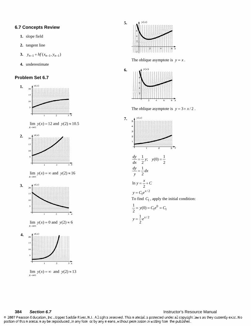
384 Section 6.7 Instructor’s Resource Manual
6.7 Concepts Review
1. slope field
2. tangent line
3. 1 1 1( , )n n ny hf x y− − −+
4. underestimate
Problem Set 6.7
1.
lim ( ) 12x
y x→∞
= and (2) 10.5y ≈
2.
lim ( )x
y x→∞
= ∞ and (2) 16y ≈
3.
lim ( ) 0x
y x→∞
= and (2) 6y ≈
4.
lim ( )x
y x→∞
= ∞ and (2) 13y ≈
5.
The oblique asymptote is y x= .
6.
The oblique asymptote is 3 / 2y x= + .
7.
1 1; (0)2 2
dy y ydx
= =
12
dy dxy
=
ln2xy C= +
/ 21
xy C e= To find 1C , apply the initial condition:
01 1
1 (0)2
y C e C= = =
/ 212
xy e=
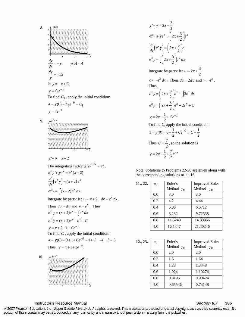
Instructor’s Resource Manual Section 6.7 385
8.
; (0) 4dy y ydx
= − =
dy dxy
= −
ln y x C= − +
1xy C e−=
To find 1C , apply the initial condition: 0
1 14 (0)y C e C−= = =
4 xy e−=
9.
' 2y y x+ = +
The integrating factor is 1dx xe e∫ = . ' ( 2)x x xe y ye e x+ = +
( ) ( 2)x xd e y x edx
= +
( 2)x xe y x e dx= +∫
Integrate by parts: let 2,u x= + xdv e dx= .
Then du dx= and xv e= . Thus ( 2)x x xe y x e e dx= + − ∫
( 2)x x xe y x e e C= + − +
2 1 xy x Ce−= + − + To find C , apply the initial condition:
04 (0) 0 1 1 3y Ce C C−= = + + = + → =
Thus, 1 3 xy x e−= + + .
10.
3' 22
y y x+ = +
3' 22
x x xe y ye x e⎛ ⎞+ = +⎜ ⎟⎝ ⎠
( ) 322
x xd e y x edx
⎛ ⎞= +⎜ ⎟⎝ ⎠
322
x xe y x e dx⎛ ⎞= +⎜ ⎟⎝ ⎠∫
Integrate by parts: let 32 ,2
u x= +
xdv e dx= . Then 2du dx= and xv e= . Thus,
32 22
x x xe y x e e dx⎛ ⎞= + −⎜ ⎟⎝ ⎠ ∫
32 22
x x xe y x e e C⎛ ⎞= + − +⎜ ⎟⎝ ⎠
122
xy x Ce−= − +
To find C, apply the initial condition: 01 13 (0) 0
2 2y Ce C−= = − + = −
Thus 72
C = , so the solution is
1 722 2
xy x e−= − +
Note: Solutions to Problems 22-28 are given along with the corresponding solutions to 11-16.
11., 22. nx Euler's Method ny
Improved Euler Method ny
0.0 3.0 3.0 0.2 4.2 4.44 0.4 5.88 6.5712 0.6 8.232 9.72538 0.8 11.5248 14.39356 1.0 16.1347 21.30246
12., 23. nx Euler's Method ny
Improved Euler Method ny
0.0 2.0 2.0 0.2 1.6 1.64 0.4 1.28 1.3448 0.6 1.024 1.10274 0.8 0.8195 0.90424 1.0 0.65536 0.74148
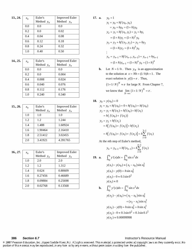
386 Section 6.7 Instructor’s Resource Manual
13., 24. nx Euler's Method ny
Improved Euler Method ny
0.0 0.0 0.0 0.2 0.0 0.02 0.4 0.04 0.08 0.6 0.12 0.18 0.8 0.24 0.32 1.0 0.40 0.50
14., 25. nx Euler's
Method ny Improved Euler Method ny
0.0 0.0 0.0 0.2 0.0 0.004 0.4 0.008 0.024 0.6 0.040 0.076 0.8 0.112 0.176 1.0 0.240 0.340
15., 26. nx Euler's Method ny
Improved Euler Method ny
1.0 1.0 1.0 1.2 1.2 1.244 1.4 1.488 1.60924 1.6 1.90464 2.16410 1.8 2.51412 3.02455 2.0 3.41921 4.391765
16., 27. nx Euler's Method ny
Improved Euler Method ny
1.0 2.0 2.0 1.2 1.2 1.312 1.4 0.624 0.80609 1.6 0.27456 0.46689 1.8 0.09884 0.25698 2.0 0.02768 0.13568
17. a. 0 1y = 1 0 0 0
0 0 0
( , )(1 )
y y hf x yy hy h y
= += + = +
2 1 1 1 1 12
1 0
( , )
(1 ) (1 )
y y hf x y y hy
h y h y
= + = +
= + = +
3 2 2 2 2 2
32 0
( , )
(1 ) (1 )
y y hf x y y hy
h y h y
= + = +
= + = +
( )
1 1 1 1 1
1 0
( , )
(1 ) (1 ) 1
n n n n n nnn
n
y y hf x y y hy
h y h y h
− − − − −
−
= + = +
= + = + = +
b. Let 1/N h= . Then Ny is an approximation to the solution at (1/ ) 1x Nh h h= = = . The exact solution is (1)y e= . Thus,
( )1 1/ NN e+ ≈ for large N. From Chapter 7,
we know that ( )lim 1 1/ N
NN e
→∞+ = .
18. 0 0( ) 0y y x= = 1 0 0 0 0( ) 0 ( ) ( )y y hf x hf x hf x= + = + =
( )
2 1 1 0 1
0 1
( ) ( ) ( )( ) ( )
y y hf x hf x hf xh f x f x
= + = +
= +
[ ]
[ ]
3 2 2
0 1 23 1
0 1 20
( )( ) ( ) ( )
( ) ( ) ( ) ( )ii
y y hf xh f x f x hf x
h f x f x f x h f x−
=
= +
= + +
= + + = ∑
At the nth step of Euler's method,
1
1 10
( ) ( )n
n n n ii
y y hf x h f x−
− −=
= + = ∑
19. a. 1 1 20 0
'( ) sinx xx x
y x dx x dx=∫ ∫
( ) 21 0 1 0 0( ) ( ) siny x y x x x x− ≈ −
21 0( ) (0) siny x y h x− =
21( ) 0 0.1sin 0y x − ≈
1( ) 0y x ≈
b. 2 2 20 0
'( ) sinx xx x
y x dx x dx=∫ ∫
( ) 2
2 0 1 0 02
2 1 1
( ) ( ) sin
( )sin
y x y x x x x
x x x
− ≈ −
+ −
2 22 0 1( ) (0) sin siny x y h x h x− = +
2 22( ) 0 0.1sin 0 0.1sin 0.1y x − ≈ +
2( ) 0.00099998y x ≈
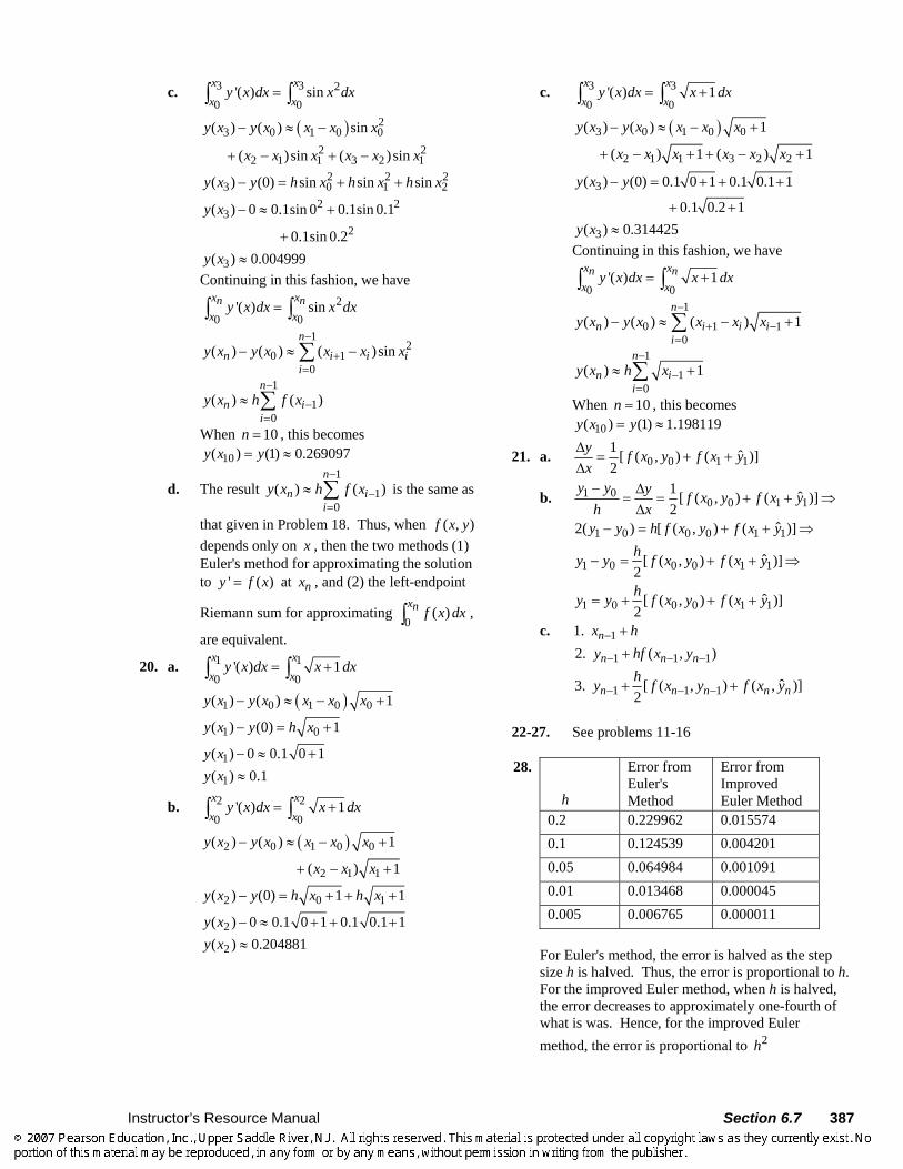
Instructor’s Resource Manual Section 6.7 387
c. 3 3 20 0
'( ) sinx xx x
y x dx x dx=∫ ∫
( ) 2
3 0 1 0 02 2
2 1 1 3 2 1
( ) ( ) sin
( )sin ( )sin
y x y x x x x
x x x x x x
− ≈ −
+ − + −
2 2 23 0 1 2( ) (0) sin sin siny x y h x h x h x− = + +
2 2
32
( ) 0 0.1sin 0 0.1sin 0.1
0.1sin 0.2
y x − ≈ +
+
3( ) 0.004999y x ≈ Continuing in this fashion, we have
20 0
'( ) sinx xn nx x
y x dx x dx=∫ ∫
1
20 1
0( ) ( ) ( )sin
n
n i i ii
y x y x x x x−
+=
− ≈ −∑
1
10
( ) ( )n
n ii
y x h f x−
−=
≈ ∑
When 10n = , this becomes 10( ) (1) 0.269097y x y= ≈
d. The result 1
10
( ) ( )n
n ii
y x h f x−
−=
≈ ∑ is the same as
that given in Problem 18. Thus, when ( , )f x y depends only on x , then the two methods (1) Euler's method for approximating the solution to ' ( )y f x= at nx , and (2) the left-endpoint
Riemann sum for approximating 0
( )xn f x dx∫ ,
are equivalent.
20. a. 1 10 0
'( ) 1x xx x
y x dx x dx= +∫ ∫
( )1 0 1 0 0( ) ( ) 1y x y x x x x− ≈ − +
1 0( ) (0) 1y x y h x− = +
1( ) 0 0.1 0 1y x − ≈ + 1( ) 0.1y x ≈
b. 2 20 0
'( ) 1x xx x
y x dx x dx= +∫ ∫
( )2 0 1 0 0
2 1 1
( ) ( ) 1
( ) 1
y x y x x x x
x x x
− ≈ − +
+ − +
2 0 1( ) (0) 1 1y x y h x h x− = + + +
2( ) 0 0.1 0 1 0.1 0.1 1y x − ≈ + + + 2( ) 0.204881y x ≈
c. 3 30 0
'( ) 1x xx x
y x dx x dx= +∫ ∫
( )3 0 1 0 0
2 1 1 3 2 2
( ) ( ) 1
( ) 1 ( ) 1
y x y x x x x
x x x x x x
− ≈ − +
+ − + + − +
3( ) (0) 0.1 0 1 0.1 0.1 1
0.1 0.2 1
y x y− = + + +
+ +
3( ) 0.314425y x ≈ Continuing in this fashion, we have
0 0
'( ) 1x xn nx x
y x dx x dx= +∫ ∫
1
0 1 10
( ) ( ) ( ) 1n
n i i ii
y x y x x x x−
+ −=
− ≈ − +∑
1
10
( ) 1n
n ii
y x h x−
−=
≈ +∑
When 10n = , this becomes 10( ) (1) 1.198119y x y= ≈
21. a. 0 0 1 11 ˆ[ ( , ) ( )]2
y f x y f x yx
Δ= + +
Δ
b. 1 00 0 1 1
1 0 0 0 1 1
1 0 0 0 1 1
1 0 0 0 1 1
1 ˆ[ ( , ) ( )]2
ˆ2( ) [ ( , ) ( )]
ˆ[ ( , ) ( )]2
ˆ[ ( , ) ( )]2
y y y f x y f x yh x
y y h f x y f x yhy y f x y f x y
hy y f x y f x y
− Δ= = + + ⇒
Δ− = + + ⇒
− = + + ⇒
= + + +
c. 1
1 1 1
1 1 1
1.2. ( , )
ˆ3. [ ( , ) ( , )]2
n
n n n
n n n n n
x hy hf x y
hy f x y f x y
−
− − −
− − −
+
+
+ +
22-27. See problems 11-16
28.
h
Error from Euler's Method
Error from Improved Euler Method
0.2 0.229962 0.015574 0.1 0.124539 0.004201 0.05 0.064984 0.001091 0.01 0.013468 0.000045 0.005 0.006765 0.000011
For Euler's method, the error is halved as the step
size h is halved. Thus, the error is proportional to h. For the improved Euler method, when h is halved, the error decreases to approximately one-fourth of what is was. Hence, for the improved Euler method, the error is proportional to 2h
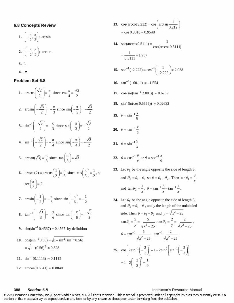
388 Section 6.8 Instructor’s Resource Manual
6.8 Concepts Review
1. – , ;2 2π π⎡ ⎤
⎢ ⎥⎣ ⎦ arcsin
2. – , ;2 2π π⎛ ⎞
⎜ ⎟⎝ ⎠
arctan
3. 1
4. π
Problem Set 6.8
1. 2arccos2 4
⎛ ⎞ π=⎜ ⎟⎜ ⎟
⎝ ⎠ since 2cos
4 2π
=
2. 3 3arcsin – – since sin – –2 3 3 2
⎛ ⎞ π π⎛ ⎞= =⎜ ⎟ ⎜ ⎟⎜ ⎟ ⎝ ⎠⎝ ⎠
3. –1 3 3sin – – since sin – –2 3 3 2
⎛ ⎞ π π⎛ ⎞= =⎜ ⎟ ⎜ ⎟⎜ ⎟ ⎝ ⎠⎝ ⎠
4. –1 2 2sin – – since sin – –2 4 4 2
⎛ ⎞ π π⎛ ⎞= =⎜ ⎟ ⎜ ⎟⎜ ⎟ ⎝ ⎠⎝ ⎠
5. arctan( 3) since tan 33 3π π⎛ ⎞= =⎜ ⎟
⎝ ⎠
6. 1 1arcsec(2) arccos since cos2 3 3 2
π π⎛ ⎞ ⎛ ⎞= = =⎜ ⎟ ⎜ ⎟⎝ ⎠ ⎝ ⎠
, so
sec 23π⎛ ⎞ =⎜ ⎟
⎝ ⎠
7. 1 1arcsin – – since sin – –2 6 6 2
π π⎛ ⎞ ⎛ ⎞= =⎜ ⎟ ⎜ ⎟⎝ ⎠ ⎝ ⎠
8. –1 3 3tan – – since tan – –3 6 6 3
⎛ ⎞ π π⎛ ⎞= =⎜ ⎟ ⎜ ⎟⎜ ⎟ ⎝ ⎠⎝ ⎠
9. –1sin(sin 0.4567) 0.4567= by definition
10. –1 2 1cos(sin 0.56) 1 sin (sin 0.56)−= − 21– (0.56) 0.828= ≈
11. 1sin (0.1113)− ≈ 0.1115
12. arccos(0.6341) ≈ 0.8840
13. 1cos(arccot 3.212) cos arctan3.212
⎛ ⎞= ⎜ ⎟⎝ ⎠
cos 0.3018 0.9548≈ ≈
14. 1sec(arccos 0.5111)cos(arccos 0.5111)
=
1 1.9570.5111
= ≈
15. –1 –1 1sec (–2.222) cos 2.038–2.222
⎛ ⎞= ≈⎜ ⎟⎝ ⎠
16. 1tan ( 60.11)− − ≈ –1.554
17. 1cos(sin(tan 2.001))− ≈ 0.6259
18. 2sin (ln(cos 0.5555)) ≈ 0.02632
19. 1sin8xθ −=
20. 1tan6xθ −=
21. 1 5sinx
θ −=
22. 1 19cos or sec9x
xθ θ− −= =
23. Let 1θ be the angle opposite the side of length 3,
and 2 1 – ,θ θ θ= so 1 2– .θ θ θ= Then 13tanx
θ =
and 21tan .x
θ = –1 –13 1tan – tan .x x
θ =
24. Let 1θ be the angle opposite the side of length 5, and 2 1θ θ θ= − , and y the length of the unlabeled
side. Then 1 2θ θ θ= − and 2 25.y x= −
1 22 2
5 5 2 2tan , tan25 25y yx x
θ θ= = = =− −
,
1 12 2
5 2tan tan25 25x x
θ − −= −− −
25. –1 2 –12 2cos 2sin – 1– 2sin sin –3 3
⎡ ⎤ ⎡ ⎤⎛ ⎞ ⎛ ⎞=⎜ ⎟ ⎜ ⎟⎢ ⎥ ⎢ ⎥⎝ ⎠ ⎝ ⎠⎣ ⎦ ⎣ ⎦
22 11– 2 –3 9
⎛ ⎞= =⎜ ⎟⎝ ⎠
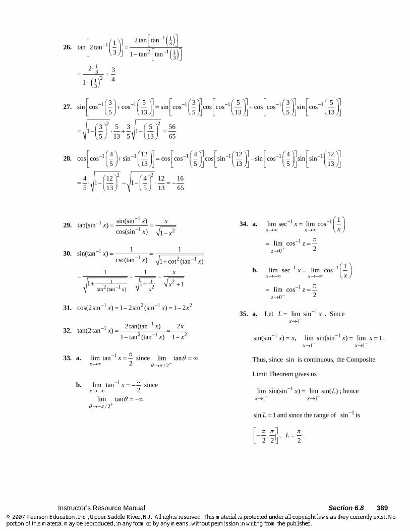
Instructor’s Resource Manual Section 6.8 389
26. ( )
( )
( )
–1 13–1
2 –1 13
13
213
2 tan tan1tan 2 tan3 1– tan tan
2 341–
⎡ ⎤⎡ ⎤⎛ ⎞ ⎣ ⎦=⎜ ⎟⎢ ⎥ ⎡ ⎤⎝ ⎠⎣ ⎦
⎣ ⎦
⋅= =
27. –1 –1 –1 –1 –1 –13 5 3 5 3 5sin cos cos sin cos cos cos cos cos sin cos5 13 5 13 5 13
⎡ ⎤ ⎡ ⎤ ⎡ ⎤ ⎡ ⎤ ⎡ ⎤⎛ ⎞ ⎛ ⎞ ⎛ ⎞ ⎛ ⎞ ⎛ ⎞ ⎛ ⎞+ = +⎜ ⎟ ⎜ ⎟ ⎜ ⎟ ⎜ ⎟ ⎜ ⎟ ⎜ ⎟⎢ ⎥ ⎢ ⎥ ⎢ ⎥ ⎢ ⎥ ⎢ ⎥⎝ ⎠ ⎝ ⎠ ⎝ ⎠ ⎝ ⎠ ⎝ ⎠ ⎝ ⎠⎣ ⎦ ⎣ ⎦ ⎣ ⎦ ⎣ ⎦ ⎣ ⎦
2 23 5 3 5 561– 1–5 13 5 13 65
⎛ ⎞ ⎛ ⎞= ⋅ + =⎜ ⎟ ⎜ ⎟⎝ ⎠ ⎝ ⎠
28. –1 –1 –1 –1 –1 –14 12 4 12 4 12cos cos sin cos cos cos sin – sin cos sin sin5 13 5 13 5 13
⎡ ⎤ ⎡ ⎤ ⎡ ⎤ ⎡ ⎤ ⎡ ⎤⎛ ⎞ ⎛ ⎞ ⎛ ⎞ ⎛ ⎞ ⎛ ⎞ ⎛ ⎞+ =⎜ ⎟ ⎜ ⎟ ⎜ ⎟ ⎜ ⎟ ⎜ ⎟ ⎜ ⎟⎢ ⎥ ⎢ ⎥ ⎢ ⎥ ⎢ ⎥ ⎢ ⎥⎝ ⎠ ⎝ ⎠ ⎝ ⎠ ⎝ ⎠ ⎝ ⎠ ⎝ ⎠⎣ ⎦ ⎣ ⎦ ⎣ ⎦ ⎣ ⎦ ⎣ ⎦
2 24 12 4 12 161– – 1– –5 13 5 13 65
⎛ ⎞ ⎛ ⎞= ⋅ ⋅ =⎜ ⎟ ⎜ ⎟⎝ ⎠ ⎝ ⎠
29. –1
–1–1 2
sin(sin )tan(sin )cos(sin ) 1–
x xxx x
= =
30. –1–1 2 –1
1 1sin(tan )csc(tan ) 1 cot (tan )
xx x
= =+
1 1 22 –1 2tan (tan )
1 1
1 1 1x x
x
x= = =
+ + +
31. –1 2 –1 2cos(2sin ) 1– 2sin (sin ) 1– 2x x x= =
32. –1
–12 –1 2
2 tan(tan ) 2tan(2 tan )1– tan (tan ) 1–
x xxx x
= =
33. a. –1lim tan2x
x→∞
π= since
/ 2lim tan
θ πθ
−→= ∞
b. –1–
lim tan –2x
x→ ∞
π= since
/ 2lim tan
θ πθ
+→−= −∞
34. a. –1 –1 1lim sec lim cosx x
xx→∞ →∞
⎛ ⎞= ⎜ ⎟⎝ ⎠
–1
0lim cos
2zz
+→
π= =
b. –1 –1– –
1lim sec lim cosx x
xx→ ∞ → ∞
⎛ ⎞= ⎜ ⎟⎝ ⎠
–1–0
lim cos 2z
z→
π= =
35. a. Let 1
1lim sin
xL x−
−→= . Since
1sin(sin ) ,x x− = 1
1 1lim sin(sin ) lim 1
x xx x−
− −→ →= = .
Thus, since sin is continuous, the Composite
Limit Theorem gives us
1
1 1lim sin(sin ) lim sin( )
x xx L−
− −→ →= ; hence
sin 1L = and since the range of 1sin− is
,2 2π π⎡ ⎤−⎢ ⎥⎣ ⎦
, 2
L π= .
390 Section 6.8 Instructor’s Resource Manual
b. Let 1
1lim sin
xL x−
+→−= . Since
1sin(sin ) ,x x− =1
1 1lim sin(sin ) lim 1
x xx x−
+ +→− →−= = − .
Thus, since sin is continuous, the Composite Limit Theorem gives us
1
1 1lim sin(sin ) lim sin( )
x xx L−
+ +→− →−= ;
hence sin 1L = − and since the range of 1sin− is
,2 2π π⎡ ⎤−⎢ ⎥⎣ ⎦
, 2
L π= − .
36. No. Since 1sin x− is not defined on (1, )∞ ,
1
1lim sin
xx−
+→ does not exist so neither can the
two-sided limit 1
1lim sin
xx−
→.
37. Let 1( ) sinf x y x−= = ; then the slope of the
tangent line to the graph of y at c is
2
1( )1
f cc
′ =−
. Hence, 1
lim ( )c
f c−→
′ = ∞ so
that the tangent lines approach the vertical.
38.
39. ln(2 sin )y x= + . Let 2 sinu x= + ; then lny u= so by the Chain Rule
1 1 cos2 sin
cos2 sin
dy dy du du xdx du dx u dx x
xx
⎛ ⎞ ⎛ ⎞= = = ⋅⎜ ⎟ ⎜ ⎟+⎝ ⎠ ⎝ ⎠
=+
40. tan tan tan 2tan secx x xd de e x e xdx dx
= =
41. 2sec tan secln(sec tan )
sec tand x x xx xdx x x
++ =
+
(sec )(tan sec ) secsec tanx x x x
x x+
= =+
42. 2– csc cot – csc[– ln(csc cot )] –
csc cotd x x xx xdx x x
+ =+
csc (cot csc ) csccot cscx x x x
x x+
= =+
43. –1 22 2 4
1 4sin (2 ) 41– (2 ) 1– 4
d xx xdx x x
= ⋅ =
44. 2 2
1arccos( ) – –1– ( ) 1–
xx x
x x
d ee edx e e
= ⋅ =
45. 3 –1 3 2 –12[ tan ( )] 3 tan ( )
1 ( )
xx x
xd ex e x x edx e
= ⋅ ++
2 –12 3 tan ( )
1
xx
xxex e
e
⎡ ⎤= +⎢ ⎥
+⎢ ⎥⎣ ⎦
46. 2 22 2
2( arcsin ) arcsin1– ( )
x x xd xe x e e xdx x
= ⋅ +
24
2 arcsin1–
x xe xx
⎛ ⎞⎜ ⎟= +⎜ ⎟⎝ ⎠
47. –1 3 –1 22
1(tan ) 3(tan )1
d x xdx x
= ⋅+
–1 2
23(tan )
1x
x=
+
48. 1 2
–11
sin(cos ) 1–tan(cos )cos(cos )
d d x d xxdx dx dx xx
−
−= =
21 12 21–
2
(–2 ) – 1– 1x
x x x
x
⋅ ⋅ ⋅=
2 2
2 2 2 2
– – (1– ) 1–1– 1–
x x
x x x x= =
Instructor’s Resource Manual Section 6.8 391
49. –1 3 23 3 2
1sec ( ) 3( ) –1
d x xdx x x
= ⋅6
3
–1x x=
50. –1 3 –1 22
1(sec ) 3(sec )–1
d x xdx x x
= ⋅
–1 2
2
3(sec )
–1
x
x x=
51. –1 3 –1 22
–1 2
2
1(1 sin ) 3(1 sin )1–
3(1 sin )
1–
d x xdx x
x
x
+ = + ⋅
+=
52. 121sin
4y
x− ⎛ ⎞
= ⎜ ⎟+⎝ ⎠
Let 21
4u
x=
+; then ( )1sin ( )y u x−= so by the
Chain Rule:
2
2 22
2
2
2 24 2
2 4 2
1
1
1 2( 4)11
4
( 4) 2( 4)8 15
2
( 4) 8 15
dy dy du dudx du dx dxu
xx
x
x xxx x
x
x x x
= = ⋅ =−
⎛ ⎞−⋅ =⎜ ⎟⎜ ⎟+⎝ ⎠⎛ ⎞
− ⎜ ⎟+⎝ ⎠
⎛ ⎞ ⎛ ⎞+ −⎜ ⎟ ⋅ =⎜ ⎟⎜ ⎟⎜ ⎟ ++ + ⎝ ⎠⎝ ⎠−
+ + +
53. ( )1 2tan lny x−=
Let 2 , lnu x v u= = ; then ( )1tan ( ( ))y v u x−= so by the Chain Rule:
2
2 2 2
2 2
1 1 21
1 1 21 (ln )
2[1 (ln ) ]
dy dy dv du xdx dv du dx uv
xx x
x x
= = ⋅ ⋅ =+
⋅ ⋅ =+
+
54. 2arcsec( 1)y x x= +
( )
( )
( )
( )
2 2
22 2 2
22
2 4 2
22
2 2
22 2
arcsec( 1) arcsec( 1)
2 1 arcsec( 1)1 ( 1) 1
2 arcsec( 1)1 2
2 arcsec( 1)1 2
2arcsec( 1
1 2
dy d dx x x xdx dx dx
xx xx x
x xx x x
x xx x x
xx
x x
⎡ ⎤ ⎛ ⎞= + + ⋅ +⎜ ⎟⎢ ⎥⎣ ⎦ ⎝ ⎠⎡ ⎤⎢ ⎥= + ⋅ +⎢ ⎥
+ + −⎢ ⎥⎣ ⎦⎡ ⎤⎢ ⎥= + +⎢ ⎥
+ +⎢ ⎥⎣ ⎦⎡ ⎤⎢ ⎥= + +⎢ ⎥
+ ⋅ +⎢ ⎥⎣ ⎦⎡ ⎤⎢ ⎥= + +⎢ ⎥
+ +⎢ ⎥⎣ ⎦
)
55. cos3x dx∫
Let 3 , 3u x du dx= = ; then 1cos3 cos3 (3 )3
1 1 1cos sin sin 33 3 3
x dx x dx
u du u C x C
= =
= + = +
∫ ∫
∫
56. Let 2u x= , so 2du x dx= .
2 21sin( ) sin( ) 22
x x dx x x dx= ⋅∫ ∫
1 1sin cos2 2
u du u C= = − +∫
21 cos( )2
x C= − +
57. Let u = sin 2x, so du = 2 cos 2x dx. 1sin 2 cos 2 sin 2 (2cos 2 )2
x x dx x x dx=∫ ∫
12
u du= ∫
221 sin 2
4 4u C x C= + = +
58. Let u = cos x, so sindu x dx= − . sin 1tan ( sin )cos cos
xx dx dx x dxx x
= = − −∫ ∫ ∫
1 ln ln cos
ln sec
du u C x Cu
x C
= − = − + = − +
= +
∫
392 Section 6.8 Instructor’s Resource Manual
59. Let 2xu e= , so 22 xdu e dx= . 2 2cos( )x xe e dx∫ 2 21 cos( )(2 )
2x xe e dx= ∫
1 cos2
u du= ∫
21 1sin sin( )2 2
xu C e C= + = +
11 2 2 20 0
1cos( ) sin( )2
x x xe e dx e⎡ ⎤= ⎢ ⎥⎣ ⎦∫
2 01 1sin( ) sin( )2 2
e e⎡ ⎤= −⎢ ⎥⎣ ⎦
2sin sin1 0.02622
e −= ≈
60. Let u = sin x, so du = cos x dx. 3 3
2 2 sinsin cos3 3
u xx x dx u du C C= = + = +∫ ∫
/ 23/ 2 20
0
sin 1 1sin cos 03 3 3
xx x dxπ
π ⎡ ⎤= = − =⎢ ⎥
⎢ ⎥⎣ ⎦∫
61. 2 / 2 2 / 2
00 2
1 [arcsin ]1–
dx xx
=∫
2arcsin – arcsin 02 4
π= =
62. 22 2 1
2 22 2 2sec
1 1
dx dx xx x x x
−⎡ ⎤= = ⎣ ⎦− −
∫ ∫
1 1sec 2 sec 2− −= −
1 11 2cos cos2 2 3 4 12
− − ⎛ ⎞ π π π⎛ ⎞= − = − =⎜ ⎟⎜ ⎟ ⎜ ⎟⎝ ⎠ ⎝ ⎠
63. 11 1 1 1
21 1
1 tan tan 1 tan ( 1)1
dx xx
− − −− −
⎡ ⎤= = − −⎣ ⎦+∫
4 4 2π π π⎛ ⎞= − − =⎜ ⎟
⎝ ⎠
64. Let cos , so sin .u du dθ θ θ= = −
2 2sin 1 ( sin )
1 cos 1 cosd dθ θ θ θ
θ θ= − −
+ +∫ ∫
12
1 tan1
du u Cu
−= − = − ++∫
1tan (cos ) Cθ−= − + / 2/ 2 1
20 0
sin tan (cos )1 cos
dθ θ θθ
ππ −⎡ ⎤= −⎣ ⎦+∫
1 1tan 0 tan 1 04 4
− − π π= − + = − + =
65. Let u = 2x, so du = 2 dx.
2 21 1 1 2
21 4 1 (2 )dx dx
x x=
+ +∫ ∫
21 1 1 arctan2 21
du u Cu
= = ++∫
1 arctan 22
x C= +
66. Let , so x xu e du e dx= = .
2 2 21
1 1 ( ) 1
x x
x xe edx dx due e u
= =+ + +∫ ∫ ∫
= arctan u + C = arctan ex + C
67.3 212 14
231
2
2
1 1
12 9
1 12 3
x
x
dx dxx
dx
⎛ ⎞−⎜ ⎟⎝ ⎠
⎛ ⎞−⎜ ⎟⎜ ⎟
⎝ ⎠
=−
=
∫ ∫
∫
Let 3 3,2 2
u x du dx= = ; then
231
2
2
1 1 1 2 12 3 2 3 3 1x
dx duu⎛ ⎞
−⎜ ⎟⎜ ⎟⎝ ⎠
⎛ ⎞= ⎜ ⎟
⎝ ⎠ −∫ ∫
1 11 1 3sin sin3 3 2
u C x C− − ⎛ ⎞= + = +⎜ ⎟⎜ ⎟
⎝ ⎠
68. 212 9
x dxx−
∫ . Let 212 9 , 18 ;u x du x dx= − = −
then
2 2
2
1 1 ( 18 )1812 9 12 9
1 1 1 (2 )18 18
12 99
x dx dxx x
du u Cu
x C
= − −− −
⎛ ⎞= − = − +⎜ ⎟⎝ ⎠
−= − +
∫ ∫
∫
Instructor’s Resource Manual Section 6.8 393
69. 2 2
2
1 16 13 ( 6 9) 4
1( 3) 4
dx dxx x x x
dxx
=− + − + +
=− +
∫ ∫
∫
Let 3, , 2;u x du dx a= − = = then
12 2 2
1
1 1 1 tan( 3) 41 3tan2 2
udx du Ca ax u a
x C
−
−
⎛ ⎞= = +⎜ ⎟⎝ ⎠− + +
−⎛ ⎞= +⎜ ⎟⎝ ⎠
∫ ∫
70. 172
2172
2 2
2
1 12 8 25 2( 4 4 )
1 12
( 2)
dx dxx x x x
dxx ⎛ ⎞
⎜ ⎟⎝ ⎠
= =+ + + + +
+ +
∫ ∫
∫
Let 172, , ;2
u x du dx a= + = = then
172
172
2 22
1 1
1
1 1 1 12 2( 2)
1 1 1 2 2tan tan2 2 17
34 34 ( 2)tan34 17
dx duu ax
u xC Ca a
x C
− −
−
= =++ +
⎛ ⎞+⎛ ⎞⋅ + = ⋅ +⎜ ⎟⎜ ⎟ ⎜ ⎟⎝ ⎠ ⎝ ⎠⎡ ⎤⋅ +
= +⎢ ⎥⎣ ⎦
∫ ∫
71. 2
1
4 9dx
x x −∫ . Let 2 , 2 , 3u x du dx a= = = ;
then 2 2
12 2
1
1 1 (2 )4 9 2 4 9
1 1 sec
21 sec3 3
dx dxx x x x
udu C
a au u ax
C
−
−
= =− −
⎛ ⎞= + =⎜ ⎟
⎝ ⎠−⎛ ⎞
+⎜ ⎟⎝ ⎠
∫ ∫
∫
72. 2
1 12 24 9 4 9 4 9
x xdx dx dxx x x
+= +
− − −∫ ∫ ∫
These integrals are evaluated the same as those in problems 67 and 68 (with a constant of 4 rather than 12). Thus
2 12
1 1 1 34 9 sin9 3 24 9
x xdx x Cx
−+ ⎛ ⎞= − − + +⎜ ⎟⎝ ⎠−
∫
73. The top of the picture is 7.6 ft above eye level, and the bottom of the picture is 2.6 ft above eye level. Let 1θ be the angle between the viewer’s line of sight to the top of the picture and the horizontal. Then call 2 1θ θ θ= − , so 1 2θ θ θ= − .
1 27.6 2.6tan ; tan ;b b
θ θ= =
1 17.6 2.6tan tanb b
θ − −= −
If b = 12.9, 0.3335 or 19.1θ ≈ ° .
74. a. Restrict 2x to[0, ]π , i.e., restrict x to 0, .2π⎡ ⎤
⎢ ⎥⎣ ⎦
Then y = 3 cos 2x
cos 23y x=
2 arccos3yx =
–1 1( ) arccos2 3
yx f y= =
–1 1( ) arccos2 3
xf x =
b. Restrict 3x to – , ,2 2π π⎡ ⎤
⎢ ⎥⎣ ⎦ i.e., restrict x to
– , 6 6π π⎡ ⎤
⎢ ⎥⎣ ⎦
Then y = 2 sin 3x
sin 32y x=
3 arcsin2yx =
–1 1( ) arcsin3 2
yx f y= =
–1 1( ) arcsin3 2
xf x =
c. Restrict x to – , 2 2π π⎛ ⎞
⎜ ⎟⎝ ⎠
1 tan2
y x=
2y = tan x –1( ) arctan 2x f y y= =
–1( ) arctan 2f x x=
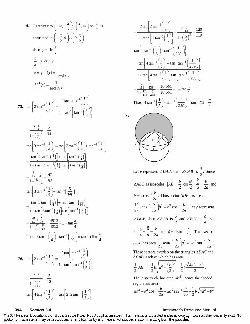
394 Section 6.8 Instructor’s Resource Manual
d. Restrict x to 2 2– , – , ⎛ ⎞ ⎛ ⎞∞ ∪ ∞⎜ ⎟ ⎜ ⎟π π⎝ ⎠ ⎝ ⎠ so 1
x is
restricted to – , 0 0, 2 2π π⎛ ⎞ ⎛ ⎞∪⎜ ⎟ ⎜ ⎟
⎝ ⎠ ⎝ ⎠
then 1sinyx
=
1 arcsin yx
=
1 1( )arcsin
x f yy
−= =
1 1( )arcsin
f xx
− =
75.
–1
–1
2 –1
12 tan tan41tan 2 tan
4 11– tan tan4
⎡ ⎤⎛ ⎞⎜ ⎟⎢ ⎥⎡ ⎤⎛ ⎞ ⎝ ⎠⎣ ⎦=⎜ ⎟⎢ ⎥ ⎡ ⎤⎛ ⎞⎝ ⎠⎣ ⎦
⎜ ⎟⎢ ⎥⎝ ⎠⎣ ⎦
( )
14
214
2 8151–
⋅= =
–1 –1 –11 1 1tan 3tan tan 2 tan tan4 4 4
⎡ ⎤ ⎡ ⎤⎛ ⎞ ⎛ ⎞ ⎛ ⎞= +⎜ ⎟ ⎜ ⎟ ⎜ ⎟⎢ ⎥ ⎢ ⎥⎝ ⎠ ⎝ ⎠ ⎝ ⎠⎣ ⎦ ⎣ ⎦
( ) ( )( ) ( )
–1 –11 14 41 –11 1
4 4
tan 2 tan tan tan
1– tan 2 tan tan tan−
⎡ ⎤ ⎡ ⎤+⎣ ⎦ ⎣ ⎦=⎡ ⎤ ⎡ ⎤⎣ ⎦ ⎣ ⎦
8 115 4
8 115 4
47521–
+= =
⋅
( ) ( )( ) ( )
–1 –1
–1 –1 514 99
–1 –1 514 99
1 5tan 3tan tan4 99
tan 3tan tan tan
1– tan 3tan tan tan
⎡ ⎤⎛ ⎞ ⎛ ⎞+⎜ ⎟ ⎜ ⎟⎢ ⎥⎝ ⎠ ⎝ ⎠⎣ ⎦⎡ ⎤ ⎡ ⎤+⎣ ⎦ ⎣ ⎦=
⎡ ⎤ ⎡ ⎤⎣ ⎦ ⎣ ⎦
47 552 99
47 552 99
4913 1 tan4913 41–
+ π= = = =
⋅
Thus, –1 –1 –11 53tan tan tan (1)4 99 4
π⎛ ⎞ ⎛ ⎞+ = =⎜ ⎟ ⎜ ⎟⎝ ⎠ ⎝ ⎠
.
76.
–1
–1
2 –1
12 tan tan51tan 2 tan
5 11– tan tan5
⎡ ⎤⎛ ⎞⎜ ⎟⎢ ⎥⎡ ⎤⎛ ⎞ ⎝ ⎠⎣ ⎦=⎜ ⎟⎢ ⎥ ⎡ ⎤⎛ ⎞⎝ ⎠⎣ ⎦
⎜ ⎟⎢ ⎥⎝ ⎠⎣ ⎦
( )15
215
2 5121–
⋅= =
–1 –11 1tan 4 tan tan 2 2 tan5 5
⎡ ⎤ ⎡ ⎤⎛ ⎞ ⎛ ⎞= ⋅⎜ ⎟ ⎜ ⎟⎢ ⎥ ⎢ ⎥⎝ ⎠ ⎝ ⎠⎣ ⎦ ⎣ ⎦
( )
–15
12252 –1
12
12 tan 2 tan 25 1201191 1–1– tan 2 tan
5
⎡ ⎤⎛ ⎞⎜ ⎟⎢ ⎥ ⋅⎝ ⎠⎣ ⎦= = =
⎡ ⎤⎛ ⎞⎜ ⎟⎢ ⎥⎝ ⎠⎣ ⎦
–1 –1
–1 –1
–1 –1
1 1tan 4 tan – tan5 239
1 1tan 4 tan – tan tan5 239
1 11 tan 4 tan tan tan5 239
⎡ ⎤⎛ ⎞ ⎛ ⎞⎜ ⎟ ⎜ ⎟⎢ ⎥⎝ ⎠ ⎝ ⎠⎣ ⎦
⎡ ⎤ ⎡ ⎤⎛ ⎞ ⎛ ⎞⎜ ⎟ ⎜ ⎟⎢ ⎥ ⎢ ⎥⎝ ⎠ ⎝ ⎠⎣ ⎦ ⎣ ⎦=
⎡ ⎤ ⎡ ⎤⎛ ⎞ ⎛ ⎞+ ⎜ ⎟ ⎜ ⎟⎢ ⎥ ⎢ ⎥⎝ ⎠ ⎝ ⎠⎣ ⎦ ⎣ ⎦
120 1119 239
120 1119 239
– 28,561 1 tan28,561 41
π= = = =
+ ⋅
Thus, –1 –1 11 14 tan – tan tan (1)5 239 4
− π⎛ ⎞ ⎛ ⎞ = =⎜ ⎟ ⎜ ⎟⎝ ⎠ ⎝ ⎠
77.
Let θ represent ,DAB∠ then CAB∠ is .2θ Since
ABCΔ is isosceles, 2, cos2 2 2
bb bAEa a
θ= = = and
–12cos .2ba
θ = Thus sector ADB has area
–1 2 2 –11 2cos cos .2 2 2
b bb ba a
⎛ ⎞ =⎜ ⎟⎝ ⎠
Let φ represent
,DCB∠ then ACB∠ is 2φ and ECA∠ is ,
4φ so
2sin4 2
b ba a
φ= = and –14sin .
2ba
φ = Thus sector
DCB has area –1 2 2 –11 4sin 2 sin .2 2 2
b ba aa a
⎛ ⎞ =⎜ ⎟⎝ ⎠
These sectors overlap on the triangles ΔDAC and ΔCAB, each of which has area
2 2 221 1 1 4 ––
2 2 2 2 2b a bAB h b a b⎛ ⎞= =⎜ ⎟
⎝ ⎠.
The large circle has area 2 ,bπ hence the shaded region has area
2 2 –1 2 –1 2 21– cos – 2 sin 4 –2 2 2b bb b a b a ba a
π +
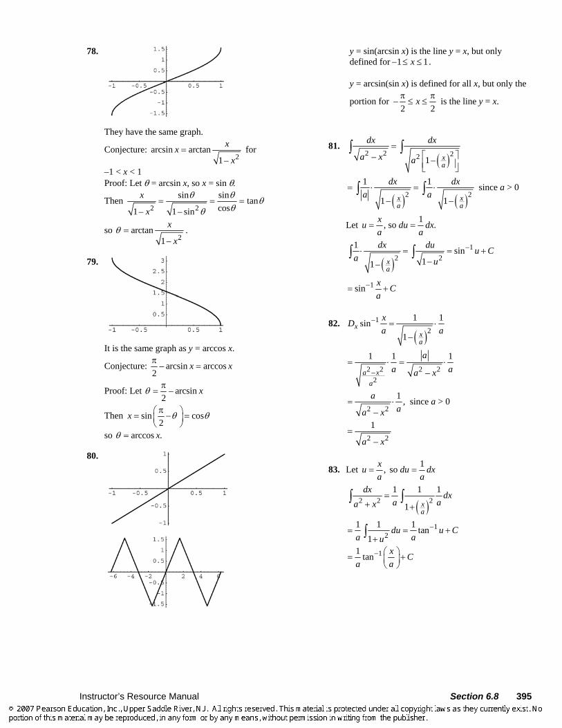
Instructor’s Resource Manual Section 6.8 395
78.
They have the same graph.
Conjecture: 2
arcsin arctan1–
xxx
= for
–1 < x < 1 Proof: Let θ = arcsin x, so x = sin θ.
Then 2 2
sin sin tancos1– 1– sin
x
x
θ θ θθθ
= = =
so 2
arctan1–
x
xθ = .
79.
It is the same graph as y = arccos x.
Conjecture: – arcsin arccos2
x xπ=
Proof: Let – arcsin2
xθ π=
Then sin cos2
x θ θπ⎛ ⎞= − =⎜ ⎟⎝ ⎠
so arccos .xθ =
80.
y = sin(arcsin x) is the line y = x, but only defined for 1 1x− ≤ ≤ . y = arcsin(sin x) is defined for all x, but only the
portion for –2 2
xπ π≤ ≤ is the line y = x.
81.
( )2 2 22– 1– xa
dx dx
a x a=
⎡ ⎤⎢ ⎥⎣ ⎦
∫ ∫
( ) ( )2 2
1 1
1– 1–x xa a
dx dxa a
= ⋅ = ⋅∫ ∫ since a > 0
Let 1, so .xu du dxa a
= =
( )1
2 2
1 sin11– x
a
dx du u Ca u
−⋅ = = +−
∫ ∫
1sin x Ca
−= +
82.
( )1
2
1 1sin1–
xxa
xDa a
− = ⋅
2 2 2 2–2
1 1 1
–a xa
aa aa x
= ⋅ = ⋅
2 2
1 ,–
aaa x
= ⋅ since a > 0
2 2
1
–a x=
83. Let 1, so xu du dxa a
= =
( )2 2 2
1 1 1
1 xa
dx dxa aa x
=+ +
∫ ∫
12
1 1 1 tan1
du u Ca au
−= = ++∫
11 tan x Ca a
− ⎛ ⎞= +⎜ ⎟⎝ ⎠
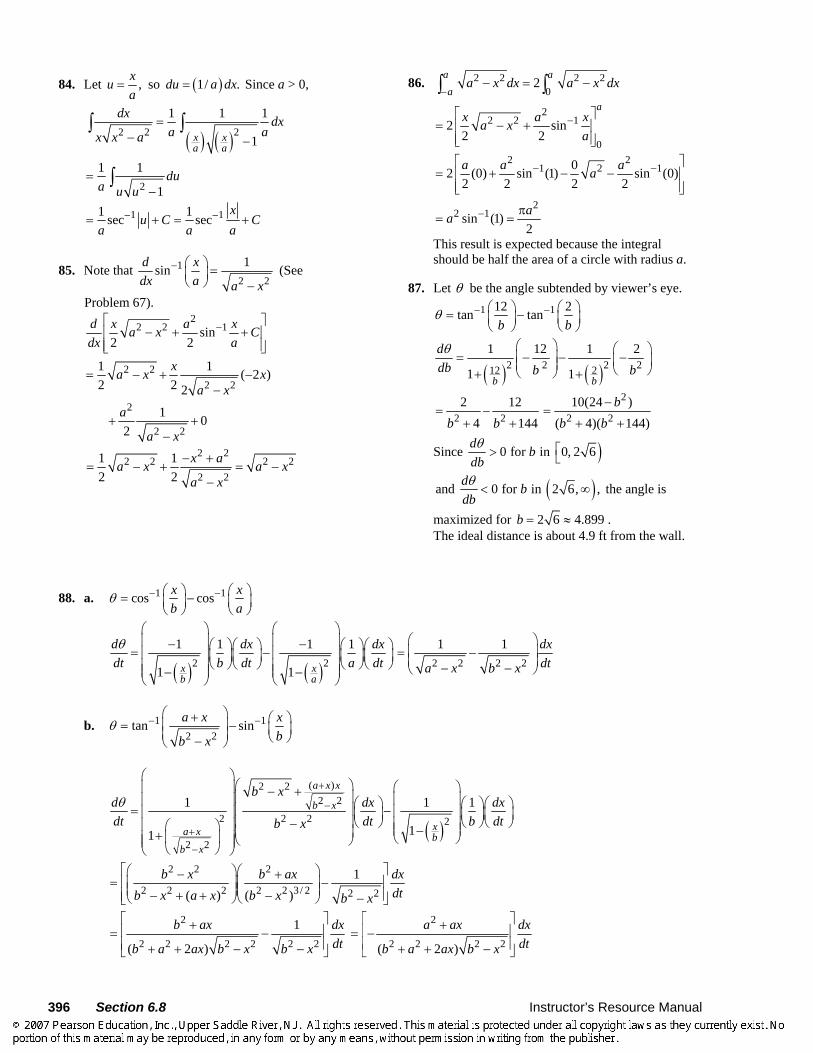
396 Section 6.8 Instructor’s Resource Manual
84. Let ,xua
= so ( )1/ .du a dx= Since a > 0,
( ) ( )2 2 2
1 1 1
1x xa a
dx dxa ax x a
=− −
∫ ∫
2
1 1
1du
a u u=
−∫
1 11 1sec secx
u C Ca a a
− −= + = +
85. Note that 12 2
1sind xdx a a x
− ⎛ ⎞ =⎜ ⎟⎝ ⎠ −
(See
Problem 67). 2
2 2 1sin2 2
d x a xa x Cdx a
−⎡ ⎤− + +⎢ ⎥
⎢ ⎥⎣ ⎦
2 22 2
2
2 2
1 1 ( 2 )2 2 2
1 02
xa x xa x
a
a x
= − + −−
+ +−
2 22 2 2 2
2 2
1 12 2
x aa x a xa x
− += − + = −
−
86. 2 2 2 20
2a aa
a x dx a x dx−
− = −∫ ∫
2
2 2 1
0
2 sin2 2
ax a xa x
a−⎡ ⎤
= − +⎢ ⎥⎢ ⎥⎣ ⎦
2 21 2 102 (0) sin (1) sin (0)
2 2 2 2a a aa− −⎡ ⎤
= + − −⎢ ⎥⎢ ⎥⎣ ⎦
22 1sin (1)
2aa − π
= =
This result is expected because the integral should be half the area of a circle with radius a.
87. Let θ be the angle subtended by viewer’s eye. 1 112 2tan tan
b bθ − −⎛ ⎞ ⎛ ⎞= −⎜ ⎟ ⎜ ⎟
⎝ ⎠ ⎝ ⎠
( ) ( )2 2 2 212 2
1 12 1 2
1 1b b
ddb b bθ ⎛ ⎞ ⎛ ⎞
= − − −⎜ ⎟ ⎜ ⎟⎜ ⎟ ⎝ ⎠⎝ ⎠+ +
2 22 12
4 144b b= −
+ +
2
2 210(24 )
( 4)( 144)b
b b−
=+ +
Since )0 for in 0, 2 6 d bdbθ ⎡> ⎣
( )and 0 for in 2 6, ,d bdbθ
< ∞ the angle is
maximized for 2 6 4.899b = ≈ . The ideal distance is about 4.9 ft from the wall.
88. a. 1 1cos cosx xb a
θ − −⎛ ⎞ ⎛ ⎞= −⎜ ⎟ ⎜ ⎟⎝ ⎠ ⎝ ⎠
( ) ( )2 2
1 1 1 1
1 1x xb a
d dx dxdt b dt a dtθ
⎛ ⎞ ⎛ ⎞⎜ ⎟ ⎜ ⎟− −⎛ ⎞⎛ ⎞ ⎛ ⎞⎛ ⎞= −⎜ ⎟ ⎜ ⎟⎜ ⎟⎜ ⎟ ⎜ ⎟⎜ ⎟
⎝ ⎠⎝ ⎠ ⎝ ⎠⎝ ⎠⎜ ⎟ ⎜ ⎟⎜ ⎟ ⎜ ⎟− −⎝ ⎠ ⎝ ⎠
2 2 2 2
1 1 dxdta x b x
⎛ ⎞⎜ ⎟= −⎜ ⎟− −⎝ ⎠
b. 1 12 2
tan sina x xbb x
θ − −⎛ ⎞+ ⎛ ⎞⎜ ⎟= − ⎜ ⎟⎜ ⎟ ⎝ ⎠−⎝ ⎠
( )
( )2 22 2
2 2 2 2
2 2
1 1 1
11
a x x
b x
xa x bb x
b xd dx dxdt dt b dtb xθ
+
−
+
−
⎛ ⎞⎛ ⎞ ⎛ ⎞⎜ ⎟ − +⎜ ⎟ ⎜ ⎟⎜ ⎟ ⎛ ⎞ ⎛ ⎞⎛ ⎞⎜ ⎟= − ⎜ ⎟⎜ ⎟ ⎜ ⎟ ⎜ ⎟⎜ ⎟⎜ ⎟⎝ ⎠ ⎝ ⎠⎝ ⎠− ⎜ ⎟⎜ ⎟⎛ ⎞ ⎜ ⎟−⎜ ⎟+ ⎜ ⎟⎜ ⎟ ⎝ ⎠⎝ ⎠⎜ ⎟⎝ ⎠⎝ ⎠
2 2 2
2 2 2 2 2 3/ 2 2 2
1( ) ( )
b x b ax dxdtb x a x b x b x
⎡ ⎤⎛ ⎞⎛ ⎞− += −⎢ ⎥⎜ ⎟⎜ ⎟⎜ ⎟⎜ ⎟− + + −⎢ ⎥−⎝ ⎠⎝ ⎠⎣ ⎦
2
2 2 2 2 2 2
1
( 2 )
b ax dxdtb a ax b x b x
⎡ ⎤+⎢ ⎥= −⎢ ⎥+ + − −⎣ ⎦
2
2 2 2 2( 2 )
a ax dxdtb a ax b x
⎡ ⎤+⎢ ⎥= −⎢ ⎥+ + −⎣ ⎦
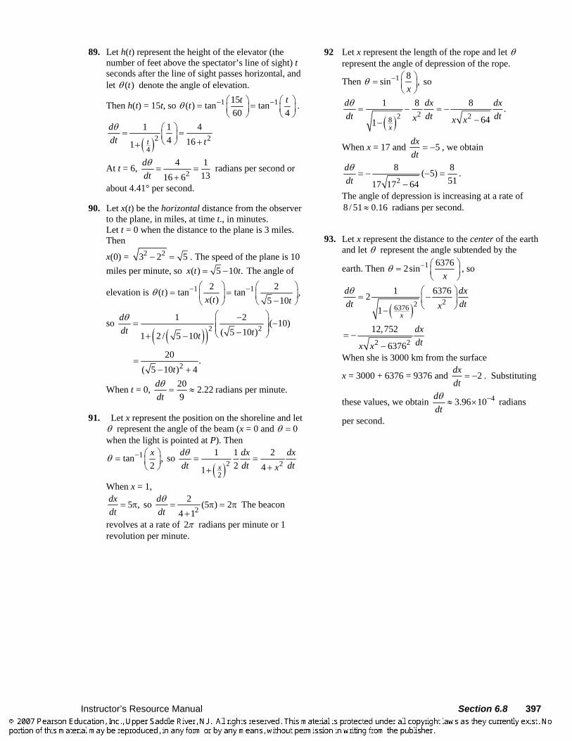
Instructor’s Resource Manual Section 6.8 397
89. Let h(t) represent the height of the elevator (the number of feet above the spectator’s line of sight) t seconds after the line of sight passes horizontal, and let ( )tθ denote the angle of elevation.
Then h(t) = 15t, so 1 115( ) tan tan60 4
t ttθ − −⎛ ⎞ ⎛ ⎞= =⎜ ⎟ ⎜ ⎟⎝ ⎠ ⎝ ⎠
.
( )2 24
1 1 44 161 t
ddt tθ ⎛ ⎞= =⎜ ⎟
⎝ ⎠ ++
At t = 6, 24 1
1316 6ddtθ
= =+
radians per second or
about 4.41° per second.
90. Let x(t) be the horizontal distance from the observer to the plane, in miles, at time t., in minutes. Let t = 0 when the distance to the plane is 3 miles. Then
x(0) = 2 23 2 5− = . The speed of the plane is 10 miles per minute, so ( ) 5 10 .x t t= − The angle of
elevation is 1 12 2( ) tan tan ,( ) 5 10
tx t t
θ − −⎛ ⎞ ⎛ ⎞= =⎜ ⎟ ⎜ ⎟
−⎝ ⎠⎝ ⎠
so ( )( )2 2
1 2 ( 10)( 5 10 )1 2 / 5 10
ddt tt
θ ⎛ ⎞−= −⎜ ⎟⎜ ⎟−⎝ ⎠+ −
220 .
( 5 10 ) 4t=
− +
When t = 0, 20 2.229
ddtθ
= ≈ radians per minute.
91. Let x represent the position on the shoreline and let θ represent the angle of the beam (x = 0 and 0θ = when the light is pointed at P). Then
( )1
2 22
1 1 2tan , so 2 2 41 x
x d dx dxdt dt dtxθθ − ⎛ ⎞= = =⎜ ⎟
⎝ ⎠ ++
When x = 1,
225 , so (5 ) 2
4 1dx ddt dt
θ= π = π = π
+ The beacon
revolves at a rate of 2π radians per minute or 1 revolution per minute.
92 Let x represent the length of the rope and let θ represent the angle of depression of the rope.
Then 1 8sin , sox
θ − ⎛ ⎞= ⎜ ⎟⎝ ⎠
( )22 28
1 8 8 .641 x
d dx dxdt dt dtx x x
θ= − = −
−−
When x = 17 and 5dxdt
= − , we obtain
2
8 8( 5)5117 17 64
ddtθ
= − − =−
.
The angle of depression is increasing at a rate of 8 / 51 0.16≈ radians per second.
93. Let x represent the distance to the center of the earth
and let θ represent the angle subtended by the
earth. Then 1 63762sinx
θ − ⎛ ⎞= ⎜ ⎟⎝ ⎠
, so
( )226376
1 637621 x
d dxdt dtxθ ⎛ ⎞
= −⎜ ⎟⎝ ⎠−
2 2
12,752
6376
dxdtx x
= −−
When she is 3000 km from the surface
x = 3000 + 6376 = 9376 and 2dxdt
= − . Substituting
these values, we obtain 43.96 10ddtθ −≈ × radians
per second.
398 Section 6.9 Instructor’s Resource Manual
6.9 Concepts Review
1. – –– ;
2 2
x x x xe e e e+
2. 2 2cosh sinh 1x x− =
3. the graph of 2 2 1x y− = , a hyperbola
4. catenary; a hanging cable or chain
Problem Set 6.9
1. – ––cosh sinh
2 2
x x x xe e e ex x ++ = +
22
xxe e= =
2. 2 –2 2 –2–cosh 2 sinh 2
2 2
x x x xe e e ex x ++ = +
222
2
xxe e= =
3. – ––cosh – sinh –
2 2
x x x xe e e ex x +=
––2
2
xxe e= =
4. 2 –2 2 –2–cosh 2 – sinh 2 –
2 2
x x x xe e e ex x +=
–2–22
2
xxe e= =
5. – – – –– –sinh cosh cosh sinh
2 2 2 2
x x y y x x y ye e e e e e e ex y x y + ++ = ⋅ + ⋅
– – – – – – – –– – – –4 4
x y x y x y x y x y x y x y x ye e e e e e e e+ + + ++ += +
–( ) –( )2 – 2 – sinh( )4 2
x y x y x y x ye e e e x y+ + + +
= = = +
6. – – – –– –sinh cosh – cosh sinh –
2 2 2 2
x x y y x x y ye e e e e e e ex y x y + += ⋅ ⋅
– – – – – – – –– – – ––4 4
x y x y x y x y x y x y x y x ye e e e e e e e+ + + ++ +=
– – – –( – )2 – 2 – sinh( – )4 2
x y x y x y x ye e e e x y+
= = =
Instructor’s Resource Manual Section 6.9 399
7. – – – –– –cosh cosh sinh sinh
2 2 2 2
x x y y x x y ye e e e e e e ex y x y + ++ = ⋅ + ⋅
– – – – – – – –– –4 4
x y x y x y x y x y x y x y x ye e e e e e e e+ + + ++ + + += +
– – –( )2 2 cosh( )4 2
x y x y x y x ye e e e x y+ + ++ +
= = = +
8. – – – –– –cosh cosh – sinh sinh –
2 2 2 2
x x y y x x y ye e e e e e e ex y x y + += ⋅ ⋅
– – – – – – – –– ––4 4
x y x y x y x y x y x y x y x ye e e e e e e e+ + + ++ + + +=
– – – –( – )2 2 cosh( – )4 2
x y x y x y x ye e e e x y++ +
= = =
9. sinhsinh
cosh coshsinhsinh
cosh cosh
tanh tanh1 tanh tanh 1
yxx y
yxx y
x yx y
++=
+ + ⋅
sinh cosh cosh sinh sinh( )cosh cosh sinh sinh cosh( )
x y x y x yx y x y x y
+ += =
+ +
= tanh (x + y)
10. sinhsinh
cosh coshsinhsinh
cosh cosh
–tanh – tanh1– tanh tanh 1–
yxx y
yxx y
x yx y
=⋅
sinh cosh – cosh sinh sinh( – )cosh cosh – sinh sinh cosh( – )
x y x y x yx y x y x y
= =
= tanh(x – y)
11. 2 sinh x cosh x = sinh x cosh x + cosh x sinh x = sinh (x + x) = sinh 2x
12. 2 2cosh sinh cosh cosh sinh sinhx x x x x x+ = + cosh( ) cosh 2x x x= + =
13. 2sinh 2sinh cosh sinh 2xD x x x x= =
14. 2cosh 2cosh sinh sinh 2xD x x x x= =
15. 2(5sinh ) 10sinh cosh 5sinh 2xD x x x x= ⋅ =
16. 3 2cosh 3cosh sinhxD x x x=
17. cosh(3 1) sinh(3 1) 3 3sinh(3 1)xD x x x+ = + ⋅ = +
18. 2 2sinh( ) cosh( ) (2 1)xD x x x x x+ = + ⋅ + 2(2 1)cosh( )x x x= + +
19. 1 coshln(sinh ) coshsinh sinhx
xD x xx x
= ⋅ =
= coth x
20. 21ln(coth ) (–csch )cothxD x x
x=
2sinh 1 1– –cosh sinh coshsinh
xx x xx
= ⋅ =
csch sechx x= −
21. 2 2( cosh ) sinh cosh 2xD x x x x x x= ⋅ + ⋅ 2 sinh 2 coshx x x x= +
22. –2 –2 –3( sinh ) cosh sinh (–2 )xD x x x x x x= ⋅ + ⋅ 2 3cosh 2 sinhx x x x− −= −
23. (cosh 3 sinh ) cosh 3 cosh sinh sinh 3 3xD x x x x x x= ⋅ + ⋅ ⋅ cosh 3 cosh 3sinh 3 sinhx x x x= +
24. (sinh cosh 4 ) sinh sinh 4 4 cosh 4 coshxD x x x x x x= ⋅ ⋅ + ⋅ = 4 sinh x sinh 4x + cosh x cosh 4x
25. 2(tanh sinh 2 ) tanh cosh 2 2 sinh 2 sechxD x x x x x x= ⋅ ⋅ + ⋅ 22 tanh cosh 2 sinh 2 sechx x x x= +
26. 2(coth 4 sinh ) coth 4 cosh sinh (–csch 4 ) 4xD x x x x x x= ⋅ + ⋅ 2cosh coth 4 – 4sinh csch 4x x x x=
400 Section 6.9 Instructor's Resource Manual
27. –1 22 2 4
1 2sinh ( ) 2( ) 1 1
xxD x x
x x= ⋅ =
+ +
28. 2
–1 3 23 2 6
1 3cosh ( ) 3( ) –1 –1
xxD x x
x x= ⋅ =
29. –12
1tanh (2 – 3) 21– (2 – 3)
xD xx
= ⋅ 2 22 2
1– (4 –12 9) –4 12 – 8x x x x= =
+ + 21–
2( – 3 2)x x=
+
30. –1 5 15
1coth ( ) tanhx xD x Dx
− ⎛ ⎞= ⎜ ⎟
⎝ ⎠
10
2 6 10 615
1 5 5–11–
x
xx x x
⎛ ⎞ ⎛ ⎞= ⋅ − = ⋅ −⎜ ⎟ ⎜ ⎟
⎝ ⎠ ⎝ ⎠⎛ ⎞⎜ ⎟⎝ ⎠
4
105–
–1x
x=
31. –1 –12
1[ cosh (3 )] 3 cosh (3 ) 1(3 ) –1
xD x x x xx
= ⋅ ⋅ + ⋅ –12
3 cosh 39 –1
x xx
= +
32. 2 –1 5 2 4 –1 55 2
1( sinh ) 5 sinh 2( ) 1
xD x x x x x xx
= ⋅ ⋅ + ⋅+
6–1 5
10
5 2 sinh1
x x xx
= ++
33. –1–1 2
1 1ln(cosh )cosh –1
xD xx x
= ⋅
2 –1
1
–1coshx x=
34. –1cosh (cos )x does not have a derivative, since 1coshuD u− is only defined for u > 1 while
cos 1x ≤ for all x.
35. 2 2tanh(cot ) sech (cot ) (– csc )xD x x x= ⋅ 2 2– csc sech (cot )x x=
36. –1 –1 1coth (tanh ) tanhtanhx xD x D
x⎛ ⎞= ⎜ ⎟⎝ ⎠
–1tanh (coth )xD x= 2
22 2
1 –csch(–csch ) 11– (coth ) –csch
xxx x
= = =
37. Area = ln 30
ln 31cosh 2 sinh 202
xdx x⎡ ⎤= ⎢ ⎥⎣ ⎦∫
2 ln 3 –2 ln 3 0 –01 – ––2 2 2
e e e e⎛ ⎞= ⎜ ⎟⎜ ⎟
⎝ ⎠
1lnln 9 91 1 1( ) 94 4 9
e e ⎛ ⎞= − = −⎜ ⎟⎝ ⎠
209
=
38. Let u = 3x + 2, so du = 3 dx. 1 1sinh(3 2) sinh cosh3 3
x dx u du u C+ = = +∫ ∫
1 cosh(3 2)3
x C= + +
39. Let 2 5, so 2u x du xdx= π + = π .
2 1cosh( 5) cosh2
x x dx u duπ + =π∫ ∫
21 1sinh sinh( 5)2 2
u C x C= + = π + +π π
40. Let 1, so 2
u z du dzz
= = .
cosh 2 cosh 2sinhz dz u du u Cz
= = +∫ ∫
2sinh z C= +
41. Let 1/ 4 –3/ 44 3
1 12 , so 2 .4 2
u z du z dz dzz
= = ⋅ =
1/ 4
4 3
sinh(2 ) 2 sinh 2coshz dz u du u Cz
= = +∫ ∫
1/ 42cosh(2 )z C= +
Instructor’s Resource Manual Section 6.9 401
42. Let ,xu e= so xdu e dx= .
sinh sinh coshx xe e dx u du u C= = +∫ ∫
cosh xe C= +
43. Let u = sin x, so du = cos x dx cos sinh(sin ) sinh coshx x dx u du u C= = +∫ ∫
= cosh(sin x) + C
44. Let ln(cosh ),u x= so 1 sinh tanh
coshdu x x dx
x= ⋅ = .
2tanh ln(cosh )
2ux x dx u du C= = +∫ ∫
21 [ln(cosh )]2
x C= +
45. Let 2ln(sinh )u x= , so
2 22
1 cosh 2 2 cothsinh
du x xdx x x dxx
= ⋅ ⋅ = .
22 2 1 1coth ln(sinh )
2 2 2ux x x dx u du C= = ⋅ +∫ ∫
2 21 [ln(sinh )]4
x C= +
46. Area = ln 5 ln 5– ln 5 0
cosh 2 2 cosh 2x dx x dx=∫ ∫
ln 5
0
12 sinh 22
x⎡ ⎤= ⎢ ⎥⎣ ⎦
2 ln 5 2ln 51sinh(2 ln 5) ( )2
e e−= = −
1lnln 25 251 1 1( ) 252 2 25
e e ⎛ ⎞= − = −⎜ ⎟⎝ ⎠
= 312 12.4825
=
47. Note that the graphs of y = sinh x and y = 0 intersect at the origin.
Area = ln 2 ln 2
00sinh [cosh ]x dx x=∫
ln 2 ln 2 0 0
2 2e e e e−+ +
= −1 1 12 12 2 4⎛ ⎞= + − =⎜ ⎟⎝ ⎠
48. tanh 0x = when sinh x = 0, which is when x = 0.
Area = 0 88 0
( tanh ) tanhx dx x dx−
− +∫ ∫
8 80 0
sinh2 tanh 2cosh
xx dx dxx
= =∫ ∫
Let u = cosh x, so du = sinh xdx. sinh 12 2 2lncosh
x dx du u Cx u
= = +∫ ∫
8 800
sinh2 2ln coshcosh
x dx xx
= ⎡ ⎤⎣ ⎦∫
2(ln cosh 8 ln1) 2 ln(cosh 8) 14.61= − = ≈
49. Volume = 1 120 0
cosh (1 cosh 2 )2
x dx x dxππ = +∫ ∫
1
0
sinh 22 2
xxπ ⎡ ⎤= +⎢ ⎥⎣ ⎦
sinh 21 02 2π ⎛ ⎞= + −⎜ ⎟⎝ ⎠
sinh 2 4.422 4π π
= + ≈
50. Volume = ln10 20
sinh xdxπ∫
2ln100 2
x xe e dx−⎛ ⎞−
= π ⎜ ⎟⎜ ⎟⎝ ⎠
∫
2 –2ln10 ln10 2 –20 0
– 2 ( – 2 )4 4
x xx xe e dx e e dx+ π
= π = +∫ ∫ln10
2 –2
0
1 1– 2 –4 2 2
x xe x eπ ⎡ ⎤= ⎢ ⎥⎣ ⎦
2 –2 ln100[ – 4 – ]
8x xe x eπ
=
1100 – 4ln10 – 35.658 100π ⎛ ⎞= ≈⎜ ⎟⎝ ⎠
51. Note that 2 21 sinh coshx x+ = and 2 1 cosh 2cosh
2xx +
=
Surface area = ( )210
2 1 dydxy dxπ +∫
1 20
2 cosh 1 sinhx x dx= π +∫
10
2 cosh coshx x dx= π∫
10
(1 cosh 2 )x dx= π +∫
1
0sinh 2 sinh 2 8.84
2 2x xπ π⎡ ⎤= π + = π+ ≈⎢ ⎥⎣ ⎦
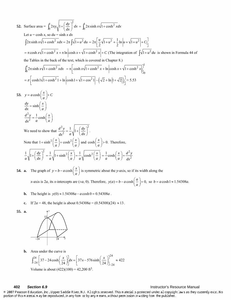
402 Section 6.9 Instructor’s Resource Manual
52. Surface area = 21
02 1 dyy dx
dx⎛ ⎞π + ⎜ ⎟⎝ ⎠∫
1 20
2 sinh 1 coshx xdx= π +∫
Let u = cosh x, so du = sinh x dx 2 22 sinh 1 cosh 2 1x xdx u duπ + = π +∫ ∫ 2 212 1 ln 1
2 2u u u u C⎡ ⎤= π + + + + +⎢ ⎥⎣ ⎦
2 2cosh 1 cosh ln cosh 1 coshx x x x C= π + + π + + + (The integration of 21 u du+∫ is shown in Formula 44 of
the Tables in the back of the text, which is covered in Chapter 8.) 1 20
2 sinh 1 coshx xdxπ +∫ 1
2 2
0cosh 1 cosh ln cosh 1 coshx x x x⎡ ⎤= π + + + +⎢ ⎥⎣ ⎦
( )2 2cosh1 1 cosh 1 ln cosh1 1 cos 1 2 ln 1 2π ⎡ ⎤= + + + + − + +⎢ ⎥⎣ ⎦≈ 5.53
53. cosh xy a Ca
⎛ ⎞= +⎜ ⎟⎝ ⎠
sinhdy xdx a
⎛ ⎞= ⎜ ⎟⎝ ⎠
2
21 coshd y xa adx
⎛ ⎞= ⎜ ⎟⎝ ⎠
We need to show that 22
21 1 .d y dya dxdx
⎛ ⎞= + ⎜ ⎟⎝ ⎠
Note that 2 21 sinh coshx xa a
⎛ ⎞ ⎛ ⎞+ =⎜ ⎟ ⎜ ⎟⎝ ⎠ ⎝ ⎠
and cosh 0.xa
⎛ ⎞ >⎜ ⎟⎝ ⎠
Therefore,
22 21 1 11 1 sinh coshdy x x
a dx a a a a⎛ ⎞ ⎛ ⎞ ⎛ ⎞+ = + =⎜ ⎟ ⎜ ⎟ ⎜ ⎟⎝ ⎠ ⎝ ⎠ ⎝ ⎠
2
21 cosh x d ya a dx
⎛ ⎞= =⎜ ⎟⎝ ⎠
54. a. The graph of cosh xy b aa
⎛ ⎞= − ⎜ ⎟⎝ ⎠
is symmetric about the y-axis, so if its width along the
x-axis is 2a, its x-intercepts are (±a, 0). Therefore, ( ) cosh 0,ay a b aa
⎛ ⎞= − =⎜ ⎟⎝ ⎠
so cosh1 1.54308 .b a a= ≈
b. The height is (0) 1.54308 cosh 0 0.54308y a a a≈ − = .
c. If 2a = 48, the height is about 0.54308a = (0.54308)(24) 13≈ .
55. a.
b. Area under the curve is 24
2424
2437 24cosh 37 576sinh 422
24 24x xdx x
−−
⎡ ⎤ ⎡ ⎤⎛ ⎞ ⎛ ⎞− = − ≈⎜ ⎟ ⎜ ⎟⎢ ⎥ ⎢ ⎥⎝ ⎠ ⎝ ⎠⎣ ⎦ ⎣ ⎦∫
Volume is about (422)(100) = 42,200 ft3.
Instructor’s Resource Manual Section 6.9 403
c. Length of the curve is 224 24 242
24 24 241 1 sinh cosh
24 24dy x xdx dx dxdx− − −
⎛ ⎞ ⎛ ⎞ ⎛ ⎞+ = + =⎜ ⎟ ⎜ ⎟ ⎜ ⎟⎝ ⎠ ⎝ ⎠ ⎝ ⎠∫ ∫ ∫
24
2424sinh 48sinh1 56.4
24x
−
⎡ ⎤⎛ ⎞= = ≈⎜ ⎟⎢ ⎥⎝ ⎠⎣ ⎦
Surface area 2(56.4)(100) 5640 ft≈ =
56. Area = cosh 2
11 cosh sinh 12
tt t x dx− −∫
cosh2 2
1
1 1 1cosh sinh 1 ln 12 2 2
tt t x x x x⎡ ⎤= − − − + −⎢ ⎥⎣ ⎦
2 21 1 1cosh sinh cosh cosh 1 ln cosh cosh 1 02 2 2
t t t t t t⎡ ⎤= − − − + − −⎢ ⎥⎣ ⎦
1 1 1 1cosh sinh cosh sinh ln cosh sinh ln2 2 2 2 2
t tt t t t t t e= − + + = =
57. a. – ––(sinh cosh )
2 2
rx x x xr e e e ex x
⎛ ⎞++ = +⎜ ⎟⎜ ⎟
⎝ ⎠
22
rxrxe e
⎛ ⎞= =⎜ ⎟⎜ ⎟⎝ ⎠
– ––sinh cosh2 2
rx rx rx rxe e e erx rx ++ = +
22
rxrxe e= =
b. – ––(cosh – sinh ) –
2 2
rx x x xr e e e ex x
⎛ ⎞+= ⎜ ⎟⎜ ⎟⎝ ⎠
––2
2
rxrxe e
⎛ ⎞= =⎜ ⎟⎜ ⎟⎝ ⎠
– ––cosh – sinh –2 2
rx rx rx rxe e e erx rx +=
––2
2
rxrxe e= =
c. ( )cos sin2 2
rix ix ix ixr e e e ex i x i
i
− −⎛ ⎞+ −+ = +⎜ ⎟⎜ ⎟
⎝ ⎠
22
rixirxe e
⎛ ⎞= =⎜ ⎟⎜ ⎟⎝ ⎠
cos sin2 2
irx irx irx irxe e e erx i rx ii
− −+ −+ = +
22
irxirxe e= =
d. ( )cos sin2 2
rix ix ix ixr e e e ex i x i
i
− −⎛ ⎞+ −− = −⎜ ⎟⎜ ⎟
⎝ ⎠
22
rixirxe e
−−⎛ ⎞
= =⎜ ⎟⎜ ⎟⎝ ⎠
cos sin2 2
irx irx irx irxe e e erx i rx ii
− −+ −− = −
22
irxirxe e
−−= =
58. a. –1(– ) tan [sinh(– )]gd t t= –1tan (– sinh )t= –1– tan (sinh ) ( )t gd t= = −
so gd is odd.
2 21 cosh[ ( )] cosh
1 sinh cosht
tD gd t tt t
= ⋅ =+
= sech t > 0 for all t, so gd is increasing. 2[ ( )] (sech ) sech tanht tD gd t D t t t= = − 2[ ( )] 0tD gd t = when tanh t = 0, since
sech t > 0 for all t. tanh t = 0 at t = 0 and tanh t < 0 for t < 0, thus 2[ ( )] 0tD gd t > for
t < 0 and 2[ ( )] 0tD gd t < for t > 0. Hence gd(t) has an inflection point at (0, gd(0)) = 1(0, tan 0)− = (0, 0).
b. If –1tan (sinh )y t= then tan y = sinh t so
2 2
tan sinhsintan 1 sinh 1
y tyy t
= =+ +
sinh tanhcosh
t tt
= = so –1sin (tanh )y t=
Also, 21 cosh
1 sinhtD y t
t= ⋅
+
2cosh 1 sech ,
coshcosht t
tt= = =
so 0
secht
y u du= ∫ by the Fundamental
Theorem of Calculus.
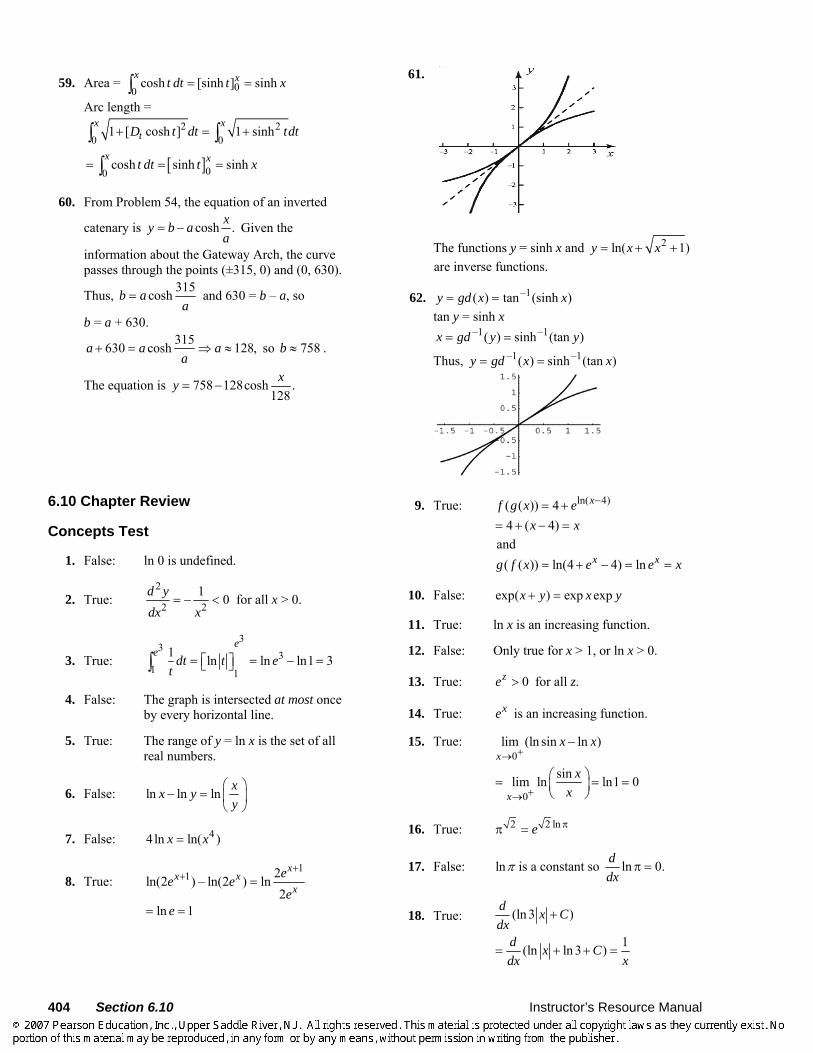
404 Section 6.10 Instructor’s Resource Manual
59. Area = 00cosh [sinh ] sinh
x xt dt t x= =∫
Arc length = 2 2
0 01 [ cosh ] 1 sinh
x xtD t dt tdt+ = +∫ ∫
[ ]00cosh sinh sinh
x xt dt t x= = =∫
60. From Problem 54, the equation of an inverted
catenary is cosh .xy b aa
= − Given the
information about the Gateway Arch, the curve passes through the points (±315, 0) and (0, 630).
Thus, 315coshb aa
= and 630 = b – a, so
b = a + 630. 315630 cosh 128,a a aa
+ = ⇒ ≈ so 758b ≈ .
The equation is 758 128cosh .128
xy = −
61.
The functions y = sinh x and 2ln( 1)y x x= + + are inverse functions.
62. –1( ) tan (sinh )y gd x x= = tan y = sinh x
–1 –1( ) sinh (tan )x gd y y= =
Thus, –1 –1( ) sinh (tan )y gd x x= =
6.10 Chapter Review
Concepts Test
1. False: ln 0 is undefined.
2. True: 2
2 21 0d y
dx x= − < for all x > 0.
3. True:
33
31 1
1 ln ln ln1 3e
edt t e
t= ⎡ ⎤ = − =⎣ ⎦∫
4. False: The graph is intersected at most once by every horizontal line.
5. True: The range of y = ln x is the set of all real numbers.
6. False: ln ln ln xx yy
⎛ ⎞− = ⎜ ⎟
⎝ ⎠
7. False: 44 ln ln( )x x=
8. True: 1
1 2ln(2 ) – ln(2 ) ln2
xx x
xee ee
++ =
ln 1e= =
9. True: ln( 4)( ( )) 44 ( 4)
xf g x ex x
−= += + − =
and ( ( )) ln(4 4) lnx xg f x e e x= + − = =
10. False: exp( ) exp expx y x y+ =
11. True: ln x is an increasing function.
12. False: Only true for x > 1, or ln x > 0.
13. True: 0ze > for all z.
14. True: xe is an increasing function.
15. True: 0
0
lim (ln sin ln )
sinlim ln ln1 0
x
x
x x
xx
+→
+→
−
⎛ ⎞= = =⎜ ⎟⎝ ⎠
16. True: 2 2 lne ππ =
17. False: lnπ is a constant so ln 0.ddx
π =
18. True: (ln 3 )
1(ln ln 3 )
d x Cdx
d x Cdx x
+
= + + =
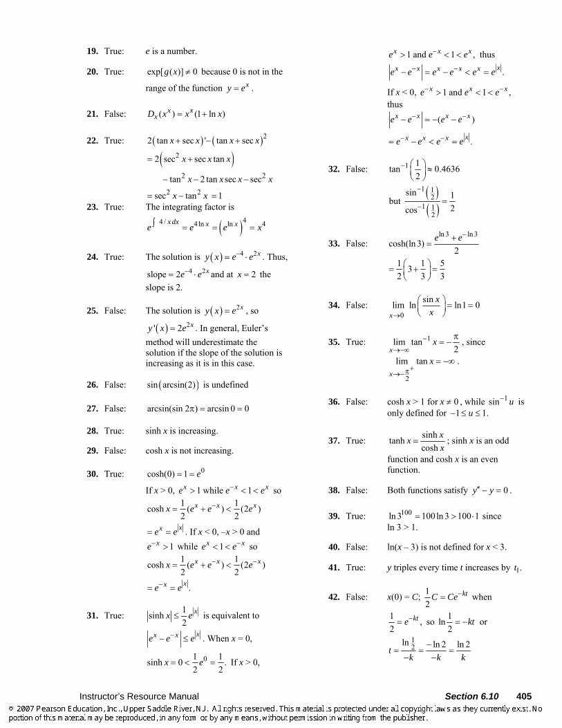
Instructor’s Resource Manual Section 6.10 405
19. True: e is a number.
20. True: exp[ ( )] 0g x ≠ because 0 is not in the
range of the function xy e= .
21. False: ( ) (1 ln )x xxD x x x= +
22. True: ( ) ( )22 tan sec ' tan secx x x x+ − +
( )2
2 2
2 sec sec tan
tan 2 tan sec sec
x x x
x x x x
= +
− − −
2 2sec tanx x= − 1= 23. True: The integrating factor is
( )44 / 4 ln ln 4x dx x xe e e x∫ = = =
24. True: The solution is ( ) 4 2xy x e e−= ⋅ . Thus, 4 2slope 2 xe e−= ⋅ and at 2x = the
slope is 2.
25. False: The solution is ( ) 2xy x e= , so
( ) 2' 2 xy x e= . In general, Euler’s method will underestimate the solution if the slope of the solution is increasing as it is in this case.
26. False: ( )sin arcsin(2) is undefined
27. False: arcsin(sin 2 ) arcsin 0 0π = =
28. True: sinh x is increasing.
29. False: cosh x is not increasing.
30. True: 0cosh(0) 1 e= =
If x > 0, 1 while 1x x xe e e−> < < so 1 1cosh ( ) (2 )2 2
x x xx e e e−= + <
xxe e= = . If x < 0, –x > 0 and 1xe− > while 1x xe e−< < so
1 1cosh ( ) (2 )2 2
x x xx e e e− −= + <
.xxe e−= =
31. True: 1sinh2
xx e≤ is equivalent to
xx xe e e−− ≤ . When x = 0,
01 1sinh 0 .2 2
x e= < = If x > 0,
1 and 1 ,x x xe e e−> < < thus
.xx x x x xe e e e e e− −− = − < =
If x < 0, 1 and 1 ,x x xe e e− −> < < thus
( )x x x xe e e e− −− = − −
.xx x xe e e e− −= − < =
32. False:
( )( )
1
1 12
1 12
1tan 0.4636 2
sin 1but 2cos
−
−
−
⎛ ⎞ ≈⎜ ⎟⎝ ⎠
=
33. False: ln 3 ln 3
cosh(ln 3)2
1 1 532 3 3
e e−+=
⎛ ⎞= + =⎜ ⎟⎝ ⎠
34. False: 0
sinlim ln ln1 0x
xx→
⎛ ⎞ = =⎜ ⎟⎝ ⎠
35. True: 1lim tan2x
x−
→−∞
π= − , since
2
lim tanx
x+π→−
= −∞ .
36. False: cosh x > 1 for 0x ≠ , while 1sin u− is only defined for 1 1.u− ≤ ≤
37. True: sinhtanhcosh
xxx
= ; sinh x is an odd
function and cosh x is an even function.
38. False: Both functions satisfy 0y y′′ − = .
39. True: 100ln 3 100ln 3 100 1= > ⋅ since ln 3 > 1.
40. False: ln(x – 3) is not defined for x < 3.
41. True: y triples every time t increases by 1.t
42. False: x(0) = C; 12
ktC Ce−= when
1 ,2
kte−= so 1ln2
kt= − or
12ln ln 2 ln 2tk k k
−= = =− −
406 Section 6.10 Instructor’s Resource Manual
43. True: ( ( ) ( )) ( ) ( )y t z t y t z t′ ′ ′+ = + ( ) ( ) ( ( ) ( ))ky t kz t k y t z t= + = +
44. False: Only true if C = 0; 1 2 1 2( ( ) ( )) ( ) ( )y t y t y t y t′ ′ ′+ = +
1 2( ) ( )ky t C ky t C= + + +
1 2( ( ) ( )) 2k y t y t C= + + .
45. False: Use the substitution u = –h. –1/ 1
0 0lim (1– ) lim (1 )h uh u
h u e→ →
= + =
by Theorem 6.5.A.
46. False: 12
0.05 0.061.051 1 1.06212
e ⎛ ⎞≈ < + ≈⎜ ⎟⎝ ⎠
47. True: If ( ) ln ,x x xxD a a a a= = then
ln a = 1, so a = e.
Sample Test Problems
1. 4
ln 4 ln ln 22x x= −
4 4ln (4 ln ln 2)2
d x d xdx dx x
= − =
2. 2 3 3 3sin ( ) 2sin( ) sin( )d dx x xdx dx
=
3 3 3 2 3 32sin( )cos( ) 6 sin( ) cos( )dx x x x x xdx
= =
3. 2 24 4 2( 4 )x x x xd de e x x
dx dx− −= −
2 4(2 4) x xx e −= −
4. 5 510 5
1log ( 1) ( 1)( 1) ln10
d dx xdx dxx
− = −−
4
55
( 1) ln10x
x=
−
5. 2tan(ln ) tan secxd de x xdx dx
= =
6. ln cot 2cot cscxd de x xdx dx
= = −
7. 2
2 sech2 tanh 2sechd d xx x xdx dx x
= =
8. 12 2
1 costanh (sin ) sin1 sin 1 sin
d d xx xdx dxx x
− = =− −
2cos sec
cosx xx
= =
9. 12
1sinh (tan ) tantan 1
d dx xdx dxx
− =+
2
2
sec
tan 1
x
x=
+
2
2
sec secsec
x xx
= =
10.
( )1
2
22sin 3 31 3
d dx xdx dx
x
− =−
2
2 3 31 3 2 3 3 9x x x x
= =− −
11. 12
1sec( ) 1
x xx x
d de edx dxe e
− =−
2 2
1
1 1
x
x x x
e
e e e= =
− −
12. ( )
2 22
2
1ln sin sin2 2sin x
d x d xdx dx
⎛ ⎞ ⎛ ⎞=⎜ ⎟ ⎜ ⎟⎝ ⎠ ⎝ ⎠
( )22
1 2sin sin2 2sin xx d x
dx⎛ ⎞ ⎛ ⎞= ⎜ ⎟ ⎜ ⎟⎝ ⎠ ⎝ ⎠
( )22
1 12sin cos cot2 2 2 2sin xx x x⎡ ⎤⎛ ⎞ ⎛ ⎞ ⎛ ⎞= =⎜ ⎟ ⎜ ⎟ ⎜ ⎟⎢ ⎥⎝ ⎠ ⎝ ⎠ ⎝ ⎠⎣ ⎦
13. 5
5 55 5
3 153ln( 1) (5 )1 1
xx x
x xd ee edx e e
+ = =+ +
14. 3ln(2 4 5)d x xdx
− +
33
1 (2 4 5)2 4 5
d x xdxx x
= − +− +
2
36 4
2 4 5x
x x−
=− +
15. cos sinx x xd de e edx dx
= −
( sin )x x de e xdx
= −
sin2
x xe ex
= −
Instructor’s Resource Manual Section 6.10 407
16. 1ln(tanh ) tanhtanh
d dx xdx x dx
=
21 sech csch sechtanh
x x xx
= =
17. 12
22cos1 ( )
d dx xdx dxx
− −=
−
2
2 1 11 2x x x x
−= = −
− −
18. 3 4 44 (3 ) (64 81 )x xd dx xdx dx
⎡ ⎤+ = +⎣ ⎦
364 ln 64 324x x= +
19. ln2csc 2cscxd de xdx dx
=
2csc cot dx x xdx
= −
csc cotx xx
= −
20. 2 / 310(log 2 )d x
dx
1/ 310 10 10
2 (log 2 ) (log 2 log )3
dx xdx
−= +
1/ 310
2 1(log 2 )3 ln10
xx
−=
3 10
23 ln10 log 2x x
=
21. 4 tan 5 sec5d x xdx
220sec 5 sec5 20 tan 5 sec5 tan 5x x x x x= + 2 220sec5 (sec 5 tan 5 )x x x= +
220sec5 (2sec 5 1)x x= −
22 2 2
122
2
444
1tan2 2
1
441
x
x
d x d xdx dx
x xx
− ⎛ ⎞ ⎛ ⎞=⎜ ⎟ ⎜ ⎟⎜ ⎟ ⎜ ⎟⎛ ⎞⎝ ⎠ ⎝ ⎠+⎜ ⎟⎝ ⎠
= =⎛ ⎞ ++⎜ ⎟⎝ ⎠
2 21 1
4
2 21
4
4tan (1) tan ( )2 2 4
4tan2 4
d x x xx xdx x
x xx
− −
−
⎡ ⎤⎛ ⎞ ⎛ ⎞ ⎛ ⎞= +⎢ ⎥⎜ ⎟ ⎜ ⎟ ⎜ ⎟⎜ ⎟ ⎜ ⎟ +⎢ ⎥ ⎝ ⎠⎝ ⎠ ⎝ ⎠⎣ ⎦
⎛ ⎞= +⎜ ⎟⎜ ⎟ +⎝ ⎠
23. 1 (1 ) lnx x xd dx edx dx
+ +=
(1 ) ln [(1 ) ln ]x x de x xdx
+= +
1 1(1)(ln ) (1 )xx x xx
+ ⎡ ⎤⎛ ⎞= + + ⎜ ⎟⎢ ⎥⎝ ⎠⎣ ⎦
1 1ln 1xx xx
+ ⎛ ⎞= + +⎜ ⎟⎝ ⎠
24. 2 2 1 2(1 ) (1 ) (1 )e ed dx e x xdx dx
−+ = + +
2 12 (1 )exe x −= +
25. Let u = 3x – 1, so du = 3 dx. 3 1 3 11 13
3 3x x ue dx e dx e du− −= =∫ ∫ ∫
3 11 13 3
u xe C e C−= + = +
Check: 3 1 3 1 3 11 1 (3 1)
3 3x x xd de C e x e
dx dx− − −⎛ ⎞+ = − =⎜ ⎟
⎝ ⎠
26. Let u = sin 3x, so du = 3 cos 3x dx. 1 16cot 3 2 3cos3 2
sin 3x dx x dx du
x u= =∫ ∫ ∫
2 ln 2ln sin 3u C x C= + = + Check:
2(2 ln sin 3 ) sin 3sin 3
d dx C xdx x dx
+ =
2(3cos3 ) 6cot 3sin 3
x xx
= =
27. Let ,xu e= so xdu e dx= .
sin sin cosx xe e dx u du u C= = − +∫ ∫
cos xe C= − + Check:
( cos ) (sin ) sinx x x x xd de C e e e edx dx
− + = =
28. Let 2 5,u x x= + − so (2 1)du x dx= + .
2 26 3 13 (2 1)
5 5x dx x dx
x x x x+
= ++ − + −∫ ∫
213 3ln 3ln 5du u C x x Cu
= = + = + − +∫
Check:
( )2 22
2
33ln 5 ( 5)5
6 35
d dx x C x xdx dxx x
xx x
+ − + = + −+ −+
=+ −
408 Section 6.10 Instructor’s Resource Manual
29. Let 3 1,xu e += + so 3xdu e dx+= . 2
33 3
1 1 1 11 1
xx
x xe dx e dx du
e e ue e
++
+ += =
+ +∫ ∫ ∫
31 ln( 1)lnxeu C C
e e
+ += + = +
Check: 3
33
ln( 1) 1 1 ( 1)1
xx
xd e dC edx e e dxe
++
+
⎛ ⎞++ = +⎜ ⎟⎜ ⎟ +⎝ ⎠
3 1 2
3 31 1
x x
x xe e ee e
+ − +
+ += =
+ +
30. Let 2 ,u x= so du = 2x dx. 2 24 cos 2 (cos )2 2 cosx x dx x x dx u du= =∫ ∫ ∫
22sin 2sinu C x C= + = + Check:
2 2 2 2(2sin ) 2cos 4 cosd dx C x x x xdx dx
+ = =
31. Let u = 2x, so du = 2 dx.
2 2
4 12 21 4 1 (2 )
dx dxx x
=− −
∫ ∫
2
121
duu
=−
∫
1 12sin 2sin 2u C x C− −= + = + Check:
12
1(2sin 2 ) 2 21 (2 )
d dx C xdx dxx
−⎛ ⎞⎜ ⎟+ =⎜ ⎟−⎝ ⎠
2
4
1 4x=
−
32. Let u = sin x, so du = cos x dx. 1
2 2cos 1 tan
1 sin 1x dx du u C
x u−= = +
+ +∫ ∫
1tan (sin )x C−= + Check:
12
1tan (sin ) sin1 sin
d dx C xdx dxx
−⎡ ⎤+ =⎣ ⎦ +
2cos
1 sinx
x=
+
33. Let u = ln x, so 1du dxx
= .
2 21 1 1
(ln ) 1 (ln )dx dx
xx x x x−
= − ⋅+ +∫ ∫
1 12
1 tan tan (ln )1
du u C x Cu
− −= − = − + = − ++∫
Check: 1
21[ tan (ln ) ] ln
1 (ln )d dx C xdx dxx
−− + = −+
21
(ln )x x x−
=+
34. Let u = x – 3, so du = dx. 2 2sech ( 3) sech tanhx dx u du u C− = = +∫ ∫
tanh( 3)x C= − + Check:
2[tanh( 3)] sech ( 3) ( 3)d dx x xdx dx
− = − −
2sech ( 3)x= −
35. ( ) cos – sin ; ( ) 0f x x x f x′ ′= = when tan x = 1,
4x π=
( ) 0f x′ > when cos x > sin x which occurs when
– .2 4
xπ π≤ <
( ) – sin – cos ; ( ) 0f x x x f x′′ ′′= = when
tan x = –1, –4
x π=
( ) 0f x′′ > when cos x < –sin x which occurs
when – – .2 4
xπ π≤ <
Increasing on – , 2 4π π⎡ ⎤
⎢ ⎥⎣ ⎦
Decreasing on , 4 2π π⎡ ⎤⎢ ⎥⎣ ⎦
Concave up on – , –2 4π π⎛ ⎞
⎜ ⎟⎝ ⎠
Concave down on – , 4 2π π⎛ ⎞
⎜ ⎟⎝ ⎠
Inflection point at – , 04π⎛ ⎞
⎜ ⎟⎝ ⎠
Global maximum at , 24π⎛ ⎞
⎜ ⎟⎝ ⎠
Instructor’s Resource Manual Section 6.10 409
Global minimum at – , –12π⎛ ⎞
⎜ ⎟⎝ ⎠
36. 2
( ) xxf xe
=
2 2
2(2 ) ( ) 2( )
( )
x x
x xe x x e x xf x
e e− −′ = =
f is increasing on [0, 2] because ( ) 0f x′ > on (0, 2). f is decreasing on ( , 0] [2, )−∞ ∪ ∞ because
( ) 0f x′ < on ( ,0) (2, ).−∞ ∪ ∞ 2 2
2(2 2 ) (2 ) 4 2( )
( )
x x
x xe x x x e x xf x
e e− − − − +′′ = =
Inflection points are at 4 16 4 2 2 2
2x ± − ⋅= = ± .
The graph of f is concave up on ( , 2 2) (2 2, )−∞ − ∪ + ∞ because ( ) 0f x′′ > on these intervals. The graph of f is concave down on (2 2, 2 2)− + because ( ) 0f x′′ < on this interval. The absolute minimum value is f(0) = 0.
The relative maximum value is 24(2) .f
e=
The inflection points are
2 2 2 2
6 4 2 6 4 22 2, and 2 2, .e e− +
⎛ ⎞ ⎛ ⎞− +− +⎜ ⎟ ⎜ ⎟⎜ ⎟ ⎜ ⎟
⎝ ⎠ ⎝ ⎠
37. a. 4 2( ) 5 6 4 4 0f x x x′ = + + ≥ > for all x, so f(x) is increasing.
b. f(1) = 7, so g(7) = 1(7) 1.f − =
c. 1 1(7)(1) 15
gf
′ = =′
38. 1012
ke=
( )12ln
0.0693110
k = ≈ −
0.06931100 ty e−= 0.069311 100 te−=
( )1100ln
66.440.06931
t = ≈−
It will take about 66.44 years.
39. 1.0 2.01.2 2.41.4 2.9761.6 3.809281.8 5.028252.0 6.83842
n nx y
40. Let x be the horizontal distance from the airplane
to the searchlight, 300.dxdt
=
1500 500tan , so tan .x x
θ θ −= =
( )2 2500
1 500
1 x
d dxdt dtxθ ⎛ ⎞= −⎜ ⎟
⎝ ⎠+
2500250,000
dxdtx
= −+
When θ = 30°, 500 500 3tan 30
x = =°
and
2 2500 (300)
(500 3) (500)ddtθ= −
+
300 3 .2000 20
= − = − The angle is decreasing at the
rate of 0.15 rad/s 8.59°/s.≈
410 Review and Preview Instructor’s Resource Manual
41. sin sin ln(cos )(cos ) x x xy x e= =
sin ln(cos ) [sin ln(cos )]x xdy de x xdx dx
=
sin ln(cos ) 1cos ln(cos ) (sin ) ( sin )
cosx xe x x x x
x+ −⎡ ⎤⎛ ⎞= ⎜ ⎟⎢ ⎥⎝ ⎠⎣ ⎦
2sin sin(cos ) cos ln(cos )
cosx xx x x
x⎡ ⎤
= −⎢ ⎥⎢ ⎥⎣ ⎦
At x = 0, 01 (1ln1 0) 0dydx
= − = .
The tangent line has slope 0, so it is horizontal: y = 1.
42. Let t represent the number of years since 1990. 1014,000 10,000 ke=
ln(1.4) 0.0336510
k = ≈
0.0336510,000 ty e= (0.03365)(20)(20) 10,000 19,601y e= ≈
The population will be about 19,600.
43. Integrating factor is x . [ ] 10; D yx y Cx−= =
44. Integrating factor is 2.x 2 3 2 –21[ ] ;
4D yx x y x Cx⎛ ⎞= = +⎜ ⎟
⎝ ⎠
45. (Linear first-order) 2 2y xy x′ + =
Integrating factor: 22xdx xe e∫ =
2 2 2 2[ ] 2 ; ;x x x xD ye xe ye e C= = +
2–1 xy Ce= + If x = 0, y = 3, then 3 = 1 + C, so C = 2.
Therefore, 2–1 2 .xy e= +
46. Integrating factor is – .axe –[ ] 1; ( )ax axD ye y e x C= = +
47. Integrating factor is –2 .xe –2 – 2[ ] ; –x x x xD ye e y e Ce= = +
48. a. ( ) 3 – 0.02Q t Q′ =
b. ( ) 0.02 3Q t Q′ + =
Integrating factor is 0.02te 0.02 0.02[ ] 3t tD Qe e=
–0.02( ) 150 tQ t Ce= + –0.02( ) 150 – 30 tQ t e= goes through (0, 120).
c. 150Q → g, as t →∞ .
Review and Preview Problems
1. 2
2
1 1sin 2 sin cos2 2
1 cos 22
u xdu dx
x dx u du u C
x C
==
= = − + =
− +
∫ ∫
2. 3
3
3 31 1 13 3 3u t
du dt
t u u te dt e du e C e C==
= = + = +∫ ∫
3. 22
2
2
1 1sin sin cos2 2
1 cos2
u xdu x dx
x x dx u du u C
x C
==
= = − + =
− +
∫ ∫
4. 2 2
236
3 31 1 16 6 6u x
du x dx
x u u xxe dx e du e C e C==
= = + = +∫ ∫
5. cos
sin
sin 1 lncos
1 1ln ln ln seccos
u tdu t dt
t dt du u Ct u
C C t Cu t
==−
= − = − + =
+ = + = +
∫ ∫
6. sin
cos
3 32 2 sinsin cos
3 3u xdu x dx
u xx x dx u du C C==
= = + = +∫ ∫
7.
( )
2 22
32 2
32 2
1 122 3
1 23
u xdu x dx
x x dx u du u C
x C
= +=
+ = = +
= + +
∫ ∫
8. 2 12
2
2
1 1 1 ln2 21
ln ln 1
u xdu x dx
x dx du u Cux
u C x C
= +=
= = ++
= + = + +
∫ ∫
Instructor’s Resource Manual Review and Preview 411
9. 1( ) (ln )(1) 1 lnf x x x xx
⎡ ⎤⎛ ⎞′ = + − =⎜ ⎟⎢ ⎥⎝ ⎠⎣ ⎦
10. 2 2
2'( ) (1)arcsin1 2 1
arcsin
x xf x xx xx
⎡ ⎤ −= + +⎢ ⎥⎢ ⎥− −⎣ ⎦
=
11.
[ ] [ ]
2
2
( ) ( 2 )(cos ) ( )( sin )
(2)(sin ) (2 )(cos ) 2( sin )
sin
f x x x x x
x x x x
x x
⎡ ⎤′ = − + − − +⎣ ⎦+ + −
=
12. ( )( ) cos sin (sin cos )
2 sin
x x
x
f x e x x e x x
e x
′ = + + −
=
13. 2cos 2 1 2sinx x= − ; thus 2 1 cos 2sin2
xx −=
14. 2cos 2 2cos 1x x= − ; thus 2 1 cos 2cos2
xx +=
15. 2
4 2 2 1 cos 2cos (cos )2
xx x +⎛ ⎞= = ⎜ ⎟⎝ ⎠
16. sin( ) sin( )sin cos2
sin(7 ) sin( ) sin 7 sinsin 3 cos 42 2
u v u vu v
x x x xx x
+ + −= ⇒
+ − −= =
17. cos( ) cos( )cos cos2
cos(8 ) cos( 2 )cos3 cos52
cos8 cos 22
u v u vu v
x xx x
x x
+ + −= ⇒
+ −=
+=
18. cos( ) cos( )sin sin2
cos( ) cos(5 )sin 2 sin 32
cos cos52
u v u vu v
x xx x
x x
− − += ⇒
− −=
−=
19. 2 2 2 2
2
( sin ) (1 sin )
cos cos
a a t a t
a t a t
− = − =
=
20. 2 2 2 2
2
( tan ) (1 tan )
sec sec
a a t a t
a t a t
+ = + =
=
21. 2 2 2 2
2
( sec ) (sec 1)
tan tan
a t a a t
a t a t
− − = − =
= ⋅
22. 0 0
1 12 21 1 112 2
2 ln 2
aa x x
aa
a
e dx e
ee
e a
− −
−
⎡ ⎤= ⇒ − = ⇒⎣ ⎦
⎡ ⎤− + = ⇒ = ⇒⎣ ⎦
= ⇒ =
∫
23. 1 1 (1 ) 2 11 (1 ) (1 )
x x xx x x x x x
− − −− = =
− − −
24. 7 8 7( 3) 8( 2)5( 2) 5( 3) 5( 2)( 3)
15 5 5(3 1)5( 2)( 3) 5( 2)( 3)
(3 1)( 2)( 3)
x xx x x x
x xx x x x
xx x
− + ++ = =
+ − + −− −
= =+ − + −
−+ −
25. 1 1 32( 1) 2( 3)x x x
− − ++ −
2 2 2
2( 1)( 3) ( 3) 3 ( 1)2 ( 1)( 3)
2( 2 3) ( 3 ) (3 3 )2 ( 1)( 3)
10 6 2(5 3)2 ( 1)( 3) 2 ( 1)( 3)(5 3)
( 1)( 3)
x x x x x xx x x
x x x x x xx x x
x xx x x x x x
xx x x
− + − − − + +=
+ −
− − − − − + +=
+ −+ +
= = =+ − + −+
+ −
26. 1 1 (2000 ) 20002000 (2000 ) (2000 )
y yy y y y y y
− ++ = =
− − −
Related Documents


![Instructor's Manual Student Assistants[1][1]](https://static.cupdf.com/doc/110x72/577d225a1a28ab4e1e972763/instructors-manual-student-assistants11.jpg)