Institute for Regulatory Policy Studies, Illinois State University Cost of Service and Rate Design Workshop Sherman Elliott Manager, State Regulatory Affairs, Midwest ISO, Inc. July 14-15, 2005 Midwest Independent Transmission System Operator, Inc. 701 City Center Drive Carmel, Indiana 46032 217.522.6674 217.522.6676 (f) [email protected]

Institute for Regulatory Policy Studies, Illinois State University Cost of Service and Rate Design Workshop Sherman Elliott Manager, State Regulatory Affairs,
Dec 19, 2015
Welcome message from author
This document is posted to help you gain knowledge. Please leave a comment to let me know what you think about it! Share it to your friends and learn new things together.
Transcript
Institute for Regulatory Policy Studies, Illinois State University
Cost of Service and Rate Design WorkshopSherman ElliottManager, State Regulatory Affairs, Midwest ISO, Inc.
July 14-15, 2005 Midwest Independent Transmission System Operator, Inc.701 City Center DriveCarmel, Indiana 46032217.522.6674217.522.6676 (f)[email protected]
2
Workplan
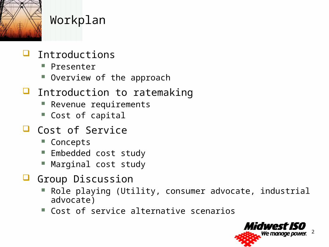
Introductions Presenter Overview of the approach
Introduction to ratemaking Revenue requirements Cost of capital
Cost of Service Concepts Embedded cost study Marginal cost study
Group Discussion Role playing (Utility, consumer advocate, industrial advocate) Cost of service alternative scenarios
3
Workplan
Next Morning’s Session
Interclass Revenue Allocation
Review of Cost Concepts Marginal Embedded
Turning Costs into Rates using different Scenarios Use results of cost studies to price services
Discuss rate effects of alternative scenarios Rate shock and Equity concerns Rationale for deviating from cost causation

Institute for Regulatory Policy Studies, Illinois State University
Introduction to Ratemaking
(6 Slides)
5
The Regulatory Equation (1)
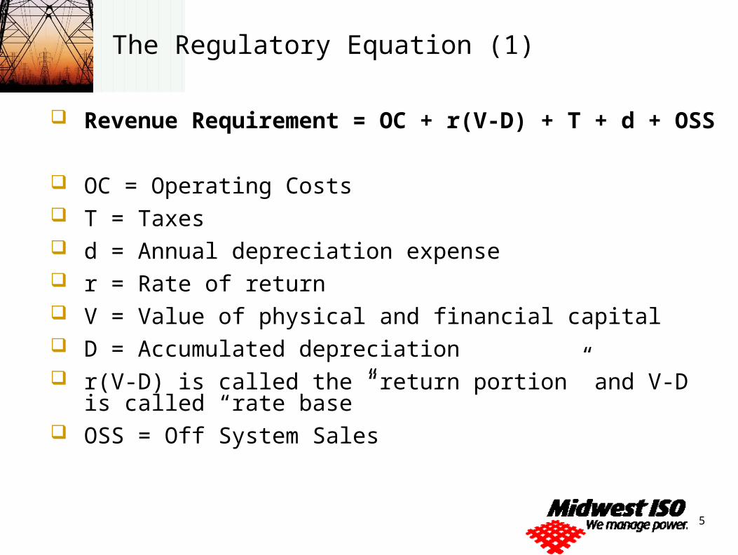
Revenue Requirement = OC + r(V-D) + T + d + OSS
OC = Operating Costs T = Taxes d = Annual depreciation expense r = Rate of return V = Value of physical and financial capital D = Accumulated depreciation r(V-D) is called the “return portion” and V-D is called “rate base” OSS = Off System Sales
6
Setting the Period of Examination (2)
Test Year - Any 12 month period used for evaluating the revenues, operating expenses, depreciation, taxes, and rate base for purposes of setting rates. Current (or historical) Test Year – A 12 month
period which reflects the actual results of current operations could be adjusted for known and measurable changes.
Future or Forecasted Test Year - A future 12 month period which reflect the anticipated results of normal operations.
7
Adjustments (3)
Pro-Forma Adjustments – known and measurable changes
Non-recurring expenses One-time basis, irregular intervals Amortized over the time period between rate cases
8
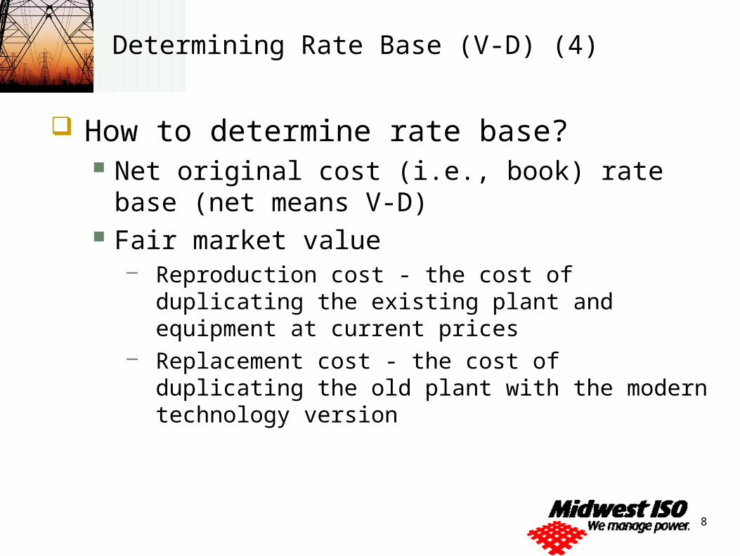
Determining Rate Base (V-D) (4)
How to determine rate base? Net original cost (i.e., book) rate base (net means
V-D) Fair market value
– Reproduction cost - the cost of duplicating the existing plant and equipment at current prices
– Replacement cost - the cost of duplicating the old plant with the modern technology version
9
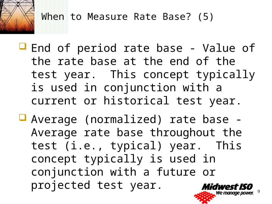
When to Measure Rate Base? (5)
End of period rate base - Value of the rate base at the end of the test year. This concept typically is used in conjunction with a current or historical test year.
Average (normalized) rate base - Average rate base throughout the test (i.e., typical) year. This concept typically is used in conjunction with a future or projected test year.
10
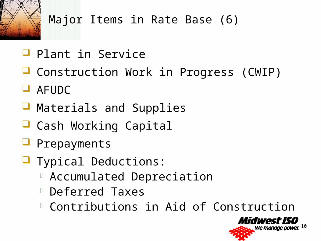
Major Items in Rate Base (6)
Plant in Service
Construction Work in Progress (CWIP)
AFUDC
Materials and Supplies
Cash Working Capital
Prepayments
Typical Deductions:» Accumulated Depreciation» Deferred Taxes» Contributions in Aid of Construction
Institute for Regulatory Policy Studies, Illinois State University
Cost of Service
(21 Slides)
12
Introduction to Cost of Service (1)
Cost of service studies (COSS) are used to: Attribute costs to different customer classes Determine how costs will be recovered from customers
within classes Calculate costs of different services Separate costs between jurisdictions Determine revenue requirement between competitive and
monopoly services
General types of cost studies Embedded (Test year accounting costs) Marginal (Change in costs related to change in output)
13
Steps in COSS (2)
Obtain test year utility revenue requirement (generally an accounting/finance function e.g., USOA) Other revenues (e.g., off-system sales, Hub sales,
etc.) Jurisdictional revenues/costs
Determine customer classes
Allocation of costs to cost-causers
14
Customer Class Determination (3)
Attempt to group customers together that have common cost characteristics, for example, Size (volume and capacity) Type of customer and meter (residential,
commercial, industrial, electricity generation) Type of usage (space heat, non-space heat etc.) Type of load (firm, interruptible) Load factor (average usage relative to peak usage) Competitive alternatives (related to opportunity
cost)
15
Embedded Cost Studies (ECOSS) (4)
Functionalize (production, distribution, transmission etc.). For gas and electric utilities, functionalization is generally an
accounting exercise (i.e., use USOA). Exception: Electric transmission may need additional
analysis (e.g., FERC seven factor test).
Classification (demand-related, volume-related, customer-related, etc.).
Allocation. Direct assignment. Allocator (demand, energy, customers, etc.).
16
Functionalization (5)
Electric and Gas utilities Generation or gas production Distribution (low voltage lines, low pressure mains) Transmission (high voltage lines, high pressure
mains) Customer Service (costs associated with hooking
up customers, meters, service drops, etc.) General plant and administrative and general
expenses (management costs, costs of buildings and offices, etc.)
17
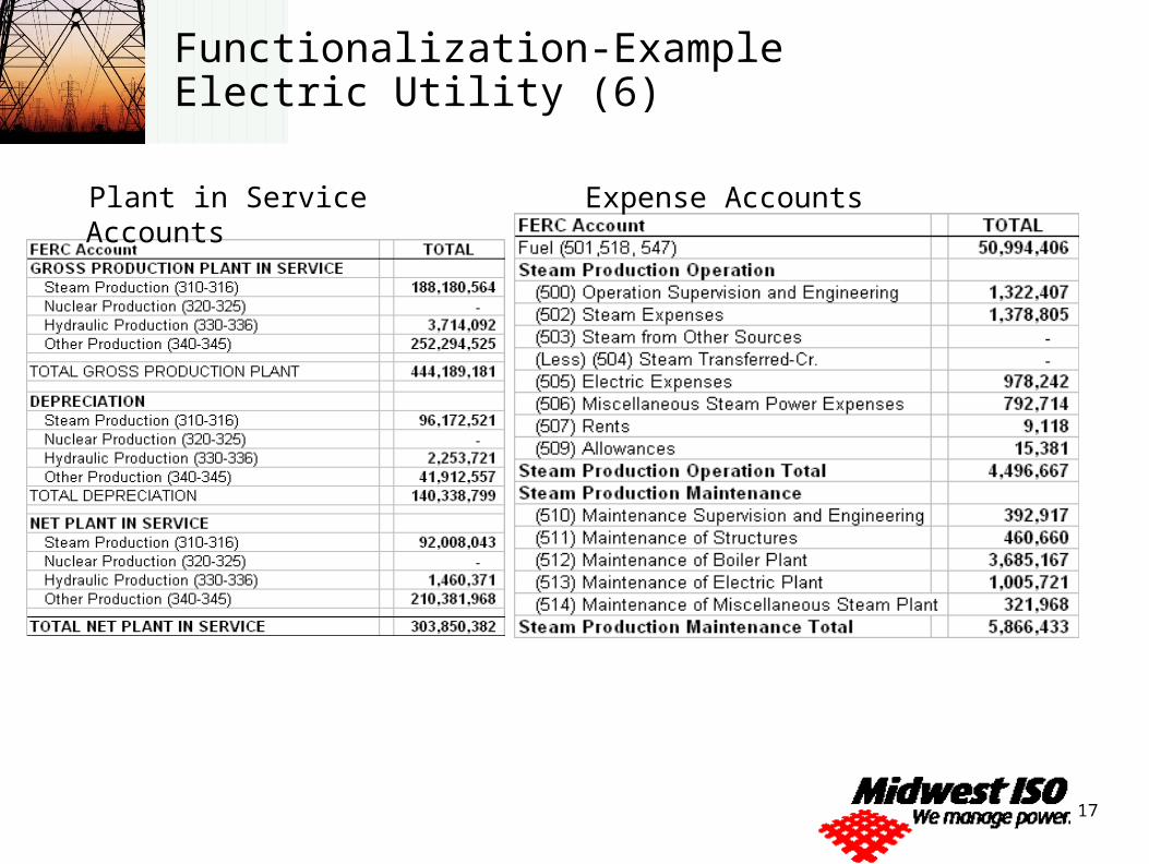
Functionalization-Example Electric Utility (6)
Plant in Service Accounts Expense Accounts
18
Classification of Costs (7)
Costs are assumed to be related to demand, energy, customer or revenues. Capacity costs (e.g., gas mains, generation plant, etc.) do
not change as output changes, but do change as the capacity of the system changes. These are fixed costs that are generally classified as demand-related (i.e., related to kW or therm capacity).
Energy-related costs change with output (e.g., fuel). These are classified as energy-related or volumetric (i.e., related to kwh or therm throughput).
Customer-related costs (e.g., meters, services) change with the number of customers added to the system.
Revenue-related costs (e.g., revenue taxes) are related to the revenue received by the company.
19
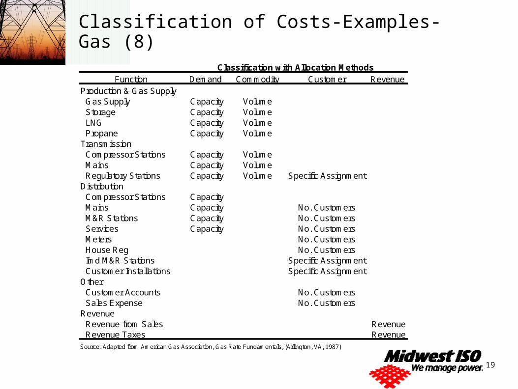
Classification of Costs-Examples-Gas (8)
Function Demand Commodity Customer Revenue Production & Gas Supply
Gas Supply Capacity VolumeStorage Capacity VolumeLNG Capacity VolumePropane Capacity Volume
TransmissionCompressor Stations Capacity VolumeMains Capacity VolumeRegulatory Stations Capacity Volume Specific Assignment
DistributionCompressor Stations CapacityMains Capacity No. CustomersM&R Stations Capacity No. CustomersServices Capacity No. CustomersMeters No. CustomersHouse Reg No. CustomersImd M&R Stations Specific AssignmentCustomer Installations Specific Assignment
OtherCustomer Accounts No. CustomersSales Expense No. Customers
RevenueRevenue from Sales RevenueRevenue Taxes Revenue
Source: Adapted from American Gas Association, Gas Rate Fundamentals, (Arlington, VA, 1987)
Classification with Allocation Methods
20
Classification-Examples (9)
Generation Plant Is generation plant entirely related to providing
capacity?
Gas mains or electric distribution Are these costs solely demand-related or is there
also a customer cost component (or are they solely customer-related)?
21
The Logic of Classification: Gas Distribution Mains (10)
What are gas distribution mains used for? Meeting peak demand?
– Historic and future planning parameters– Mains are sized to meet the highest peak demand on
the peak day Meeting average demand?
– What evidence exists concerning the reason for investment (e.g., maintenance and replacement of existing mains)
Hooking up customers?– How does investment cost change with number of
customers?
22
Classification Example: Gas Mains (11)
Zero-intercept method Statistical procedure that relates main costs
and size with number of customers
Minimum distribution system Engineering method that determines the cost
of a system of a certain size and allocates classifies those costs as customer related
23
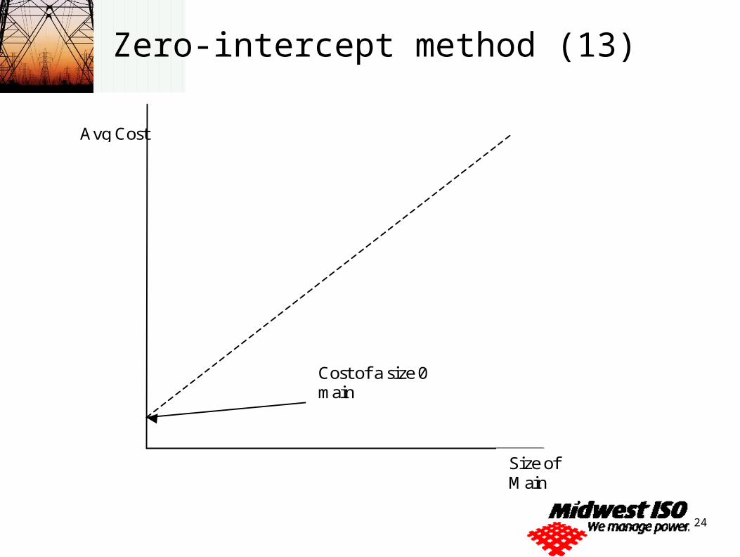
Zero-intercept method (12)
Some level of main costs are required to serve new customers
This level can be deduced from regressing unit costs of various size of mains on the sizes of mains
This suggests a level of main costs that is necessary just to expand system (i.e., just to hook up customers some level of main investment is needed)
24
Zero-intercept method (13)
Size of Main
Avg Cost
Cost of a size 0 main
25
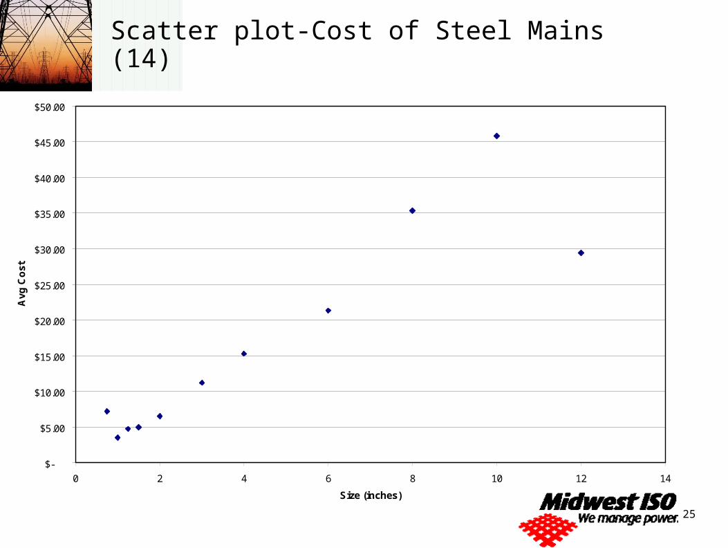
Scatter plot-Cost of Steel Mains (14)
$-
$5.00
$10.00
$15.00
$20.00
$25.00
$30.00
$35.00
$40.00
$45.00
$50.00
0 2 4 6 8 10 12 14
Size (inches)
Avg
Co
st
26
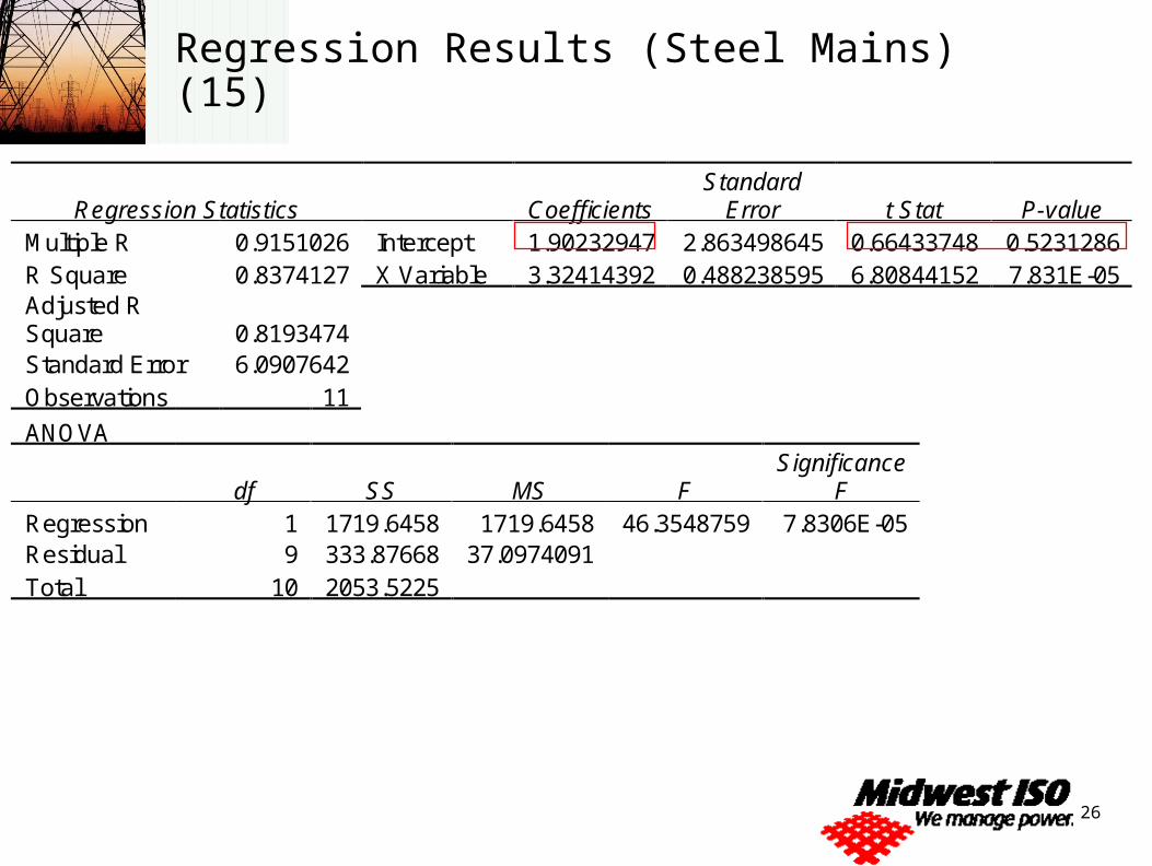
Regression Results (Steel Mains) (15)
Regression Statistics Coefficients Standard
Error t Stat P-value Multiple R 0.9151026 Intercept 1.90232947 2.863498645 0.66433748 0.5231286 R Square 0.8374127 X Variable 3.32414392 0.488238595 6.80844152 7.831E-05 Adjusted R Square 0.8193474 Standard Error 6.0907642 Observations 11
ANOVA
df SS MS F Significance
F Regression 1 1719.6458 1719.6458 46.3548759 7.8306E-05 Residual 9 333.87668 37.0974091 Total 10 2053.5225
27
Minimum Distribution Method (16)
Applies actual engineering costs of a minimum size system to determine what costs are related to customers
Question becomes what is the appropriate size of main to use to estimate the minimum size?
28
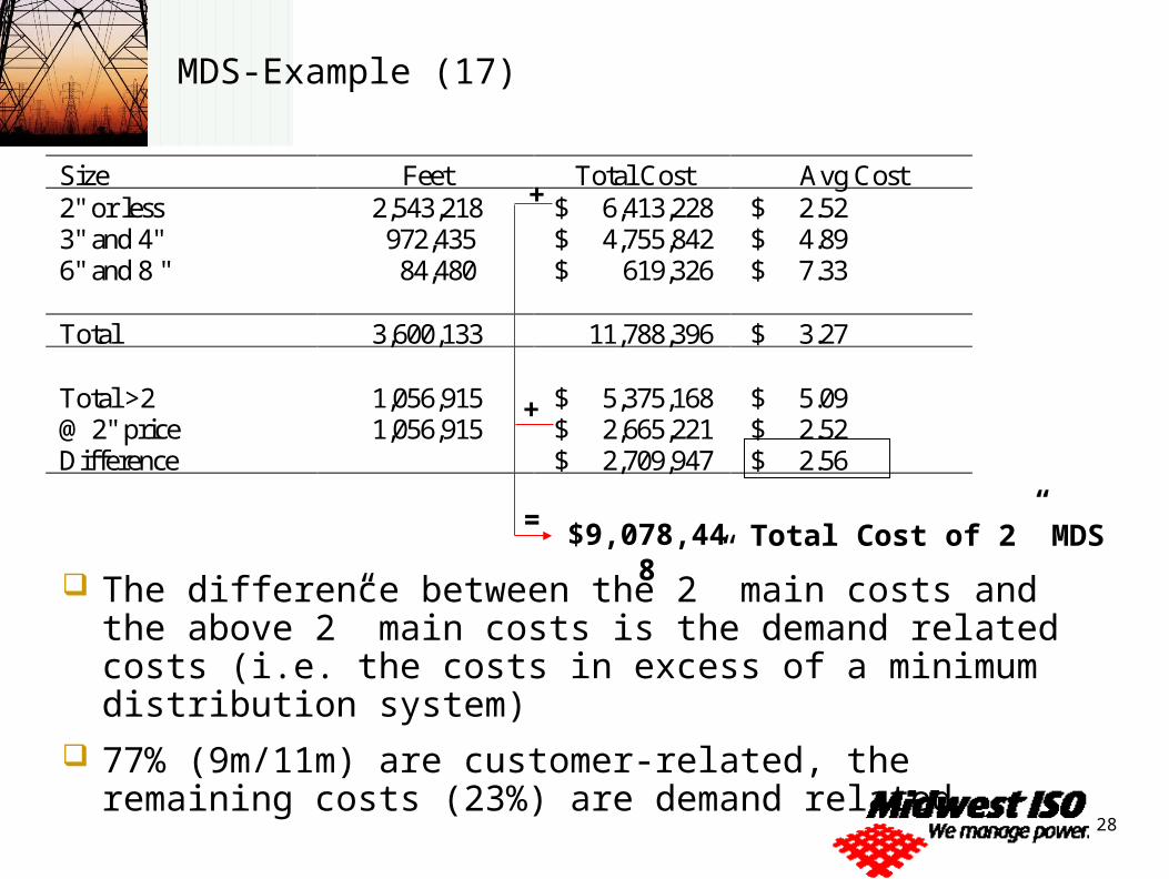
MDS-Example (17)
Size Feet Total Cost Avg Cost 2" or less 2,543,218 $ 6,413,228 $ 2.52 3" and 4" 972,435 $ 4,755,842 $ 4.89 6" and 8 " 84,480 $ 619,326 $ 7.33 Total 3,600,133 11,788,396 $ 3.27 Total >2 1,056,915 $ 5,375,168 $ 5.09 @ 2" price 1,056,915 $ 2,665,221 $ 2.52 Difference $ 2,709,947 $ 2.56
$9,078,448 Total Cost of 2” MDS
+
+
=
The difference between the 2” main costs and the above 2” main costs is the demand related costs (i.e. the costs in excess of a minimum distribution system)
77% (9m/11m) are customer-related, the remaining costs (23%) are demand related
29
Allocation to customer classes of Demand-Related Costs (18)
Peak responsibility methods Allocates capacity based on peak hour or some
average of the peak hours Customers who consume off-peak will not be
allocated these costs
Peak and average methods Uses average and peak volumes weighted by the
load factor Recognizes that some investment is for not peak
day needs
30
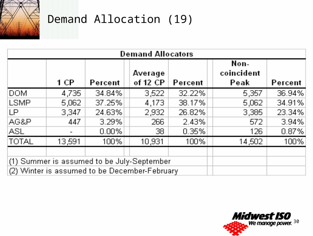
Demand Allocation (19)
31
Demand Allocation: Recognizing Energy (20)
If part of the production plant is classified as energy-related (e.g., 25%), then energy portion would be allocated based on an energy allocator.
If portions of capacity are not re-classified as energy, the energy function may still be recognized through the allocation process.
32
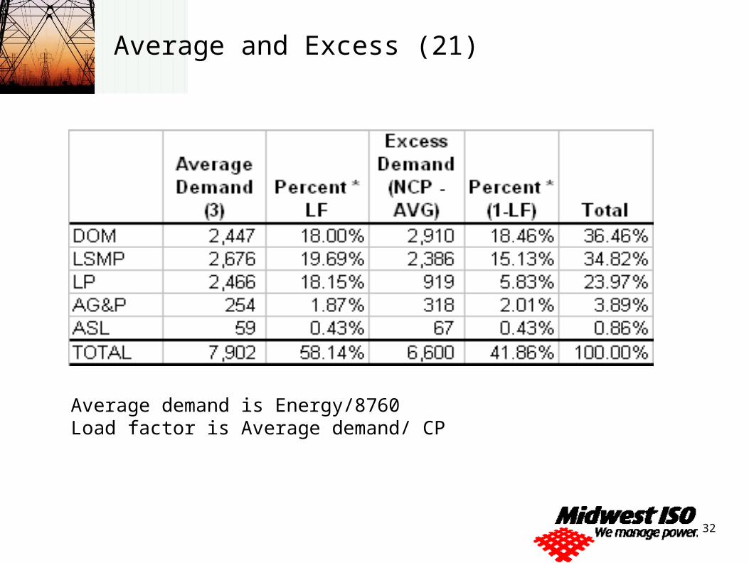
Average and Excess (21)
Average demand is Energy/8760Load factor is Average demand/ CP
Institute for Regulatory Policy Studies, Illinois State University
Marginal Cost
(35 Slides)
34
Introduction to Marginal Cost Pricing (1)
Overview of micro-economics Cost curves Revenue curves Profit maximization Why marginal costs?
Application of marginal cost to the electric industry? Marginal Generation Costs Marginal Distribution Costs Marginal Transmission Costs

35
Overview of Microeconomics (2)
Total Cost is defined as follows:
Total Cost = Fixed Costs of Production
+ Variable Cost of Production
Fixed Costs are those costs that do not change with changes in output
Variable Costs are those costs that do change with changes in output
36
Total Costs in the Electric Sector (3)
The total cost of the production of electricity is related to the capital costs of the delivery and production system and the costs of operating and maintaining the system.
Sunk Costs are those costs that cannot be avoided and could not be recovered if the firm exits the business. For example, a power plant that is built for serving a particular load center may have little value outside of providing service to those customers.
37
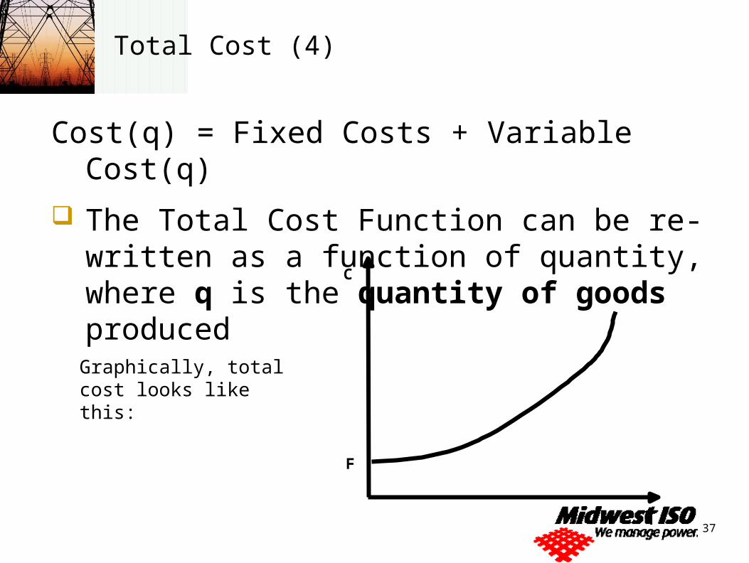
Total Cost (4)
Cost(q) = Fixed Costs + Variable Cost(q)
The Total Cost Function can be re-written as a function of quantity, where q is the quantity of goods produced
C
q
F
Graphically, total cost looks like this:
38
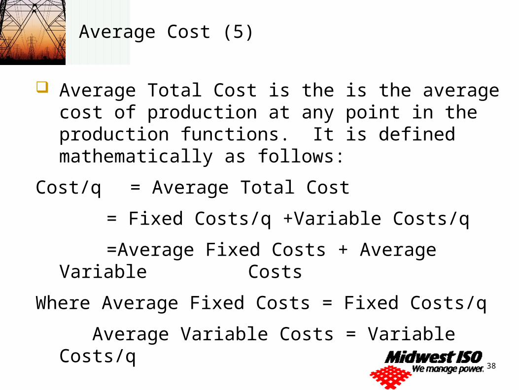
Average Cost (5)
Average Total Cost is the is the average cost of production at any point in the production functions. It is defined mathematically as follows:
Cost/q = Average Total Cost
= Fixed Costs/q +Variable Costs/q
=Average Fixed Costs + Average Variable Costs
Where Average Fixed Costs = Fixed Costs/q
Average Variable Costs = Variable Costs/q
39
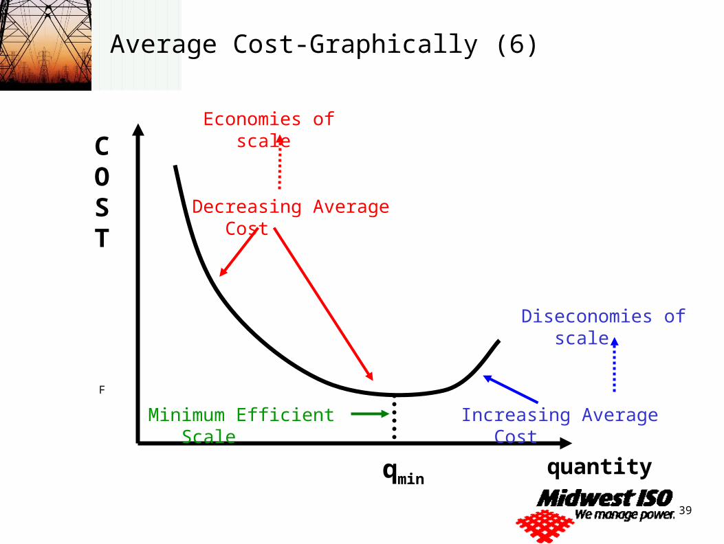
Average Cost-Graphically (6)
Economies of scale
quantity
COST
F
qmin
Decreasing Average Cost
Increasing Average Cost
Diseconomies of scale
Minimum Efficient Scale
40
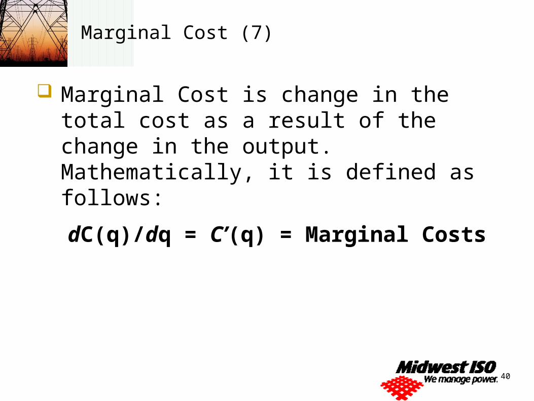
Marginal Cost (7)
Marginal Cost is change in the total cost as a result of the change in the output. Mathematically, it is defined as follows:
dC(q)/dq = C’(q) = Marginal Costs
41
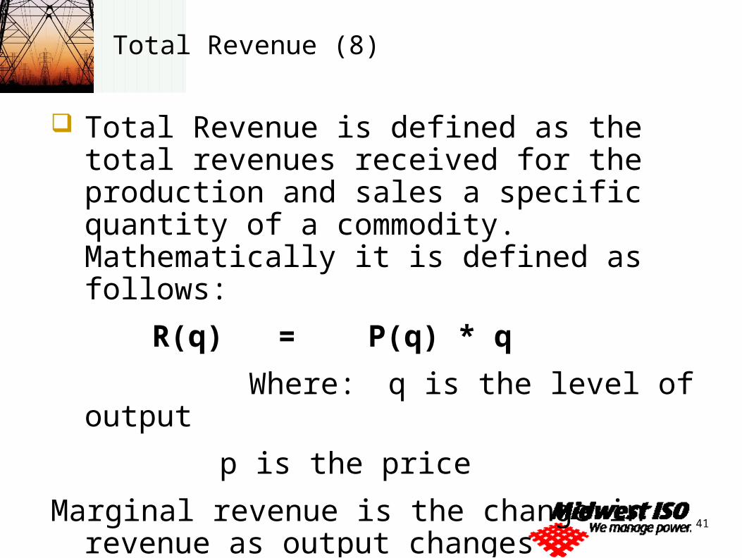
Total Revenue (8)
Total Revenue is defined as the total revenues received for the production and sales a specific quantity of a commodity. Mathematically it is defined as follows:
R(q) = P(q) * q
Where: q is the level of output
p is the price
Marginal revenue is the change in revenue as output changes
42
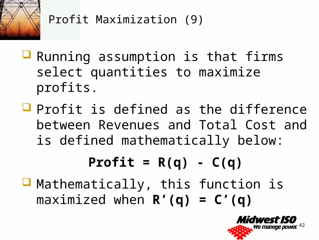
Profit Maximization (9)
Running assumption is that firms select quantities to maximize profits.
Profit is defined as the difference between Revenues and Total Cost and is defined mathematically below:
Profit = R(q) - C(q)
Mathematically, this function is maximized when R’(q) = C’(q)
43
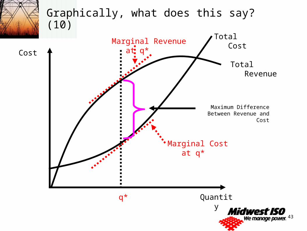
Graphically, what does this say? (10)
Cost
Quantity
Total Cost
q*
Marginal Cost at q*
Marginal Revenue at q*
Total Revenue
Maximum Difference Between Revenue and Cost
44
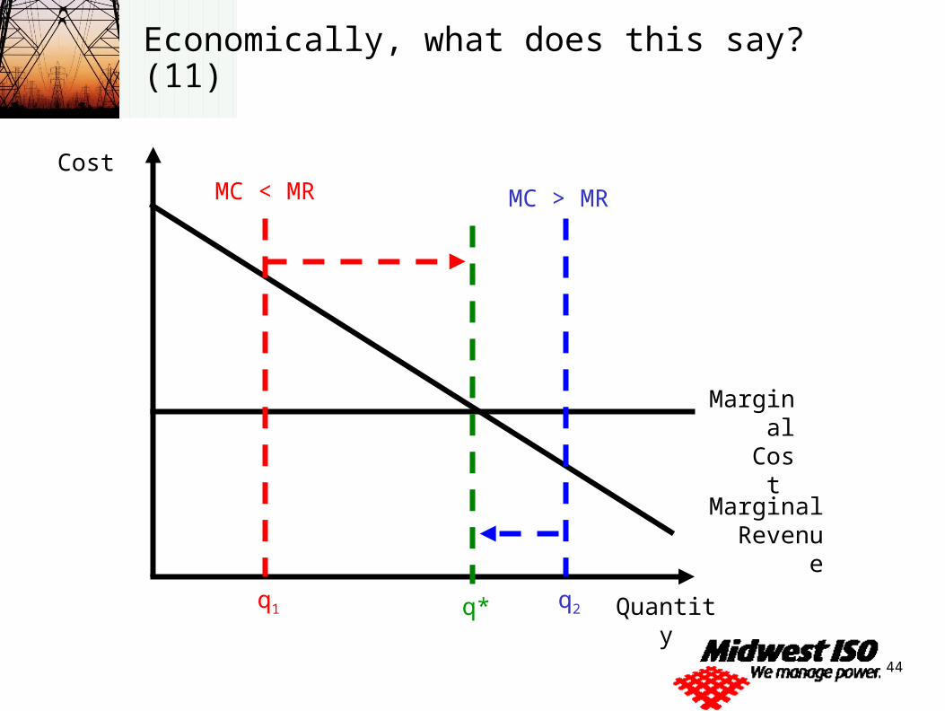
Economically, what does this say? (11)
Cost
Quantity
Marginal Cost
Marginal Revenue
q1 q2q*
MC < MR MC > MR
45
Why use marginal cost? (12)
Competitive markets price based on marginal cost Efficiency in production Efficiency in consumption Maximizes social welfare
More accurately follows utility planning and investment decisions
Creates a level playing field for unbundling
46
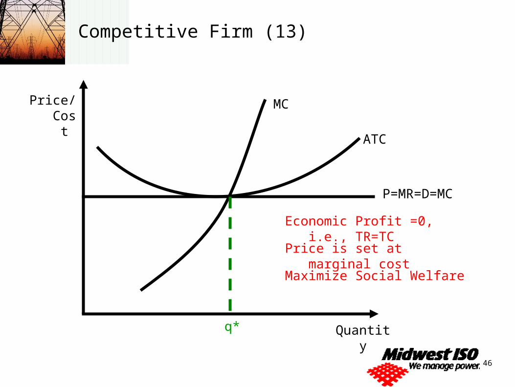
Competitive Firm (13)
Price/ Cost
Quantity
ATC
P=MR=D=MC
MC
q*
Economic Profit =0, i.e., TR=TC
Price is set at marginal cost
Maximize Social Welfare
47
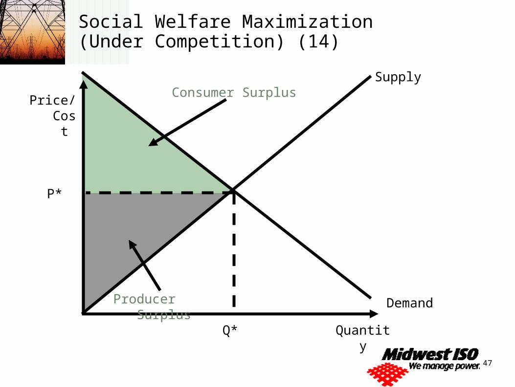
Social Welfare Maximization (Under Competition) (14)
Price/ Cost
Quantity
Demand
Supply
P*
Consumer Surplus
Producer Surplus
Q*
48
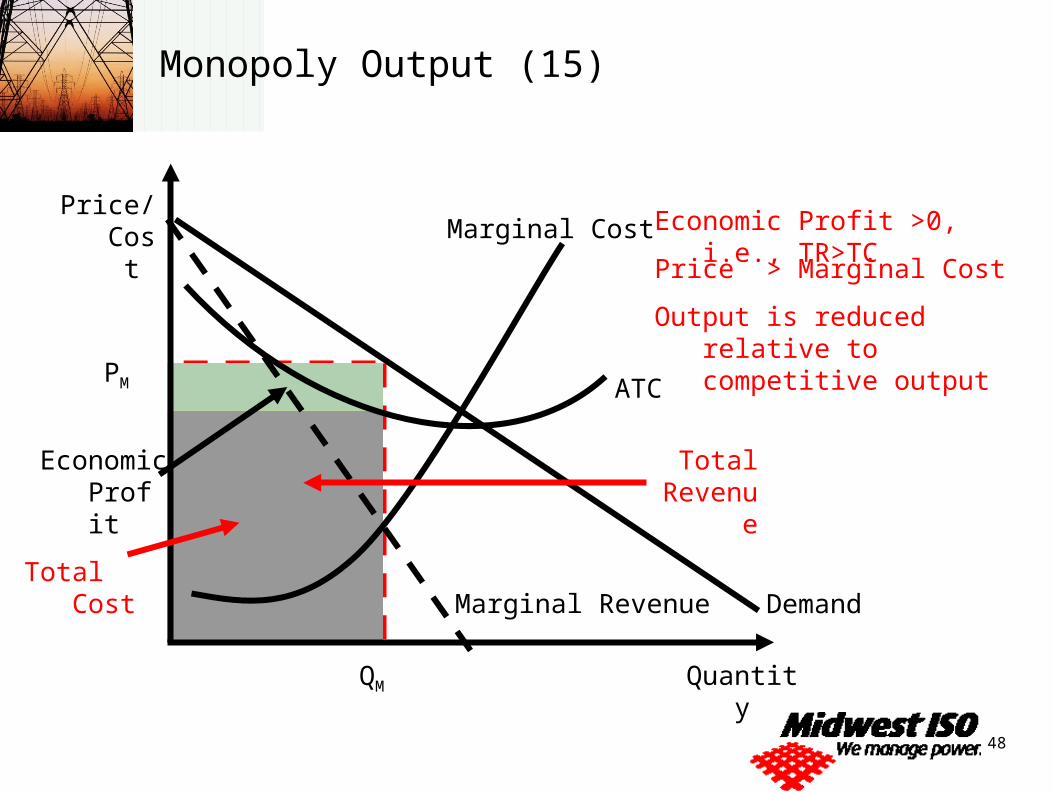
QM
PM
Economic Profit
Monopoly Output (15)
Price/ Cost
Quantity
DemandMarginal Revenue
Marginal Cost Economic Profit >0, i.e., TR>TC
ATC
Price > Marginal Cost
Output is reduced relative to competitive output
Total Revenue
Total Cost
49
QM
PM
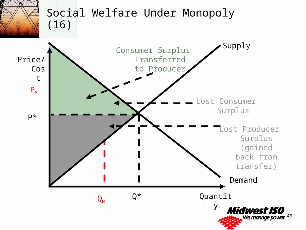
Social Welfare Under Monopoly (16)
Price/ Cost
Quantity
Demand
Supply
P*
Consumer Surplus Transferred to
Producer
Lost Producer Surplus
(gained back from transfer)
Q*
Lost Consumer Surplus
50
Use of Marginal Cost in Price Setting (17)
Short-run marginal cost would not include capital
Utilities are capital intensive
How to solve dilemma? Use of long-run marginal costs for rate making
– Long-run simply means that all inputs are variable and therefore the fixed costs of capital are variable
Translate capital investment into annual cost using the carrying charge or fixed rate charge calculation.
51
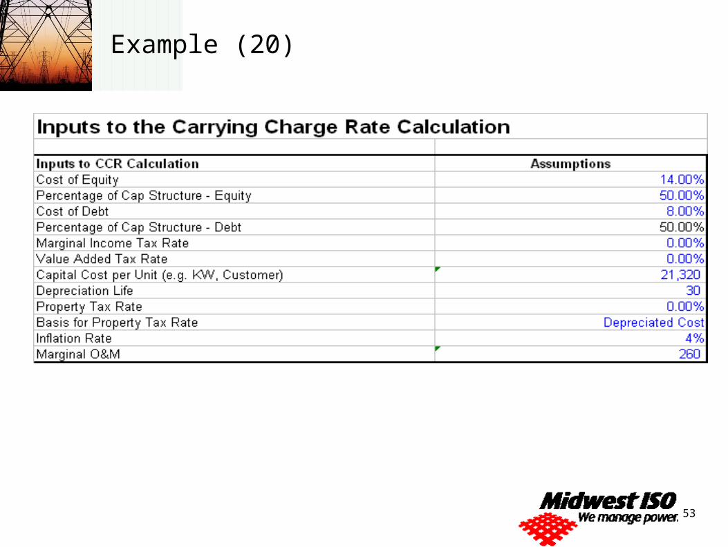
Carrying Charge Rate Calculation (18)
Fixed Charge Rate = NPV Revenue Requirements / Annuity Factor
Where
NPV Revenue Requirements is the Net Present Value of the revenue requirements over the life of the investment
and
The Annuity Factor is the sum of each year’s discount rate factor over the life of the investment
52
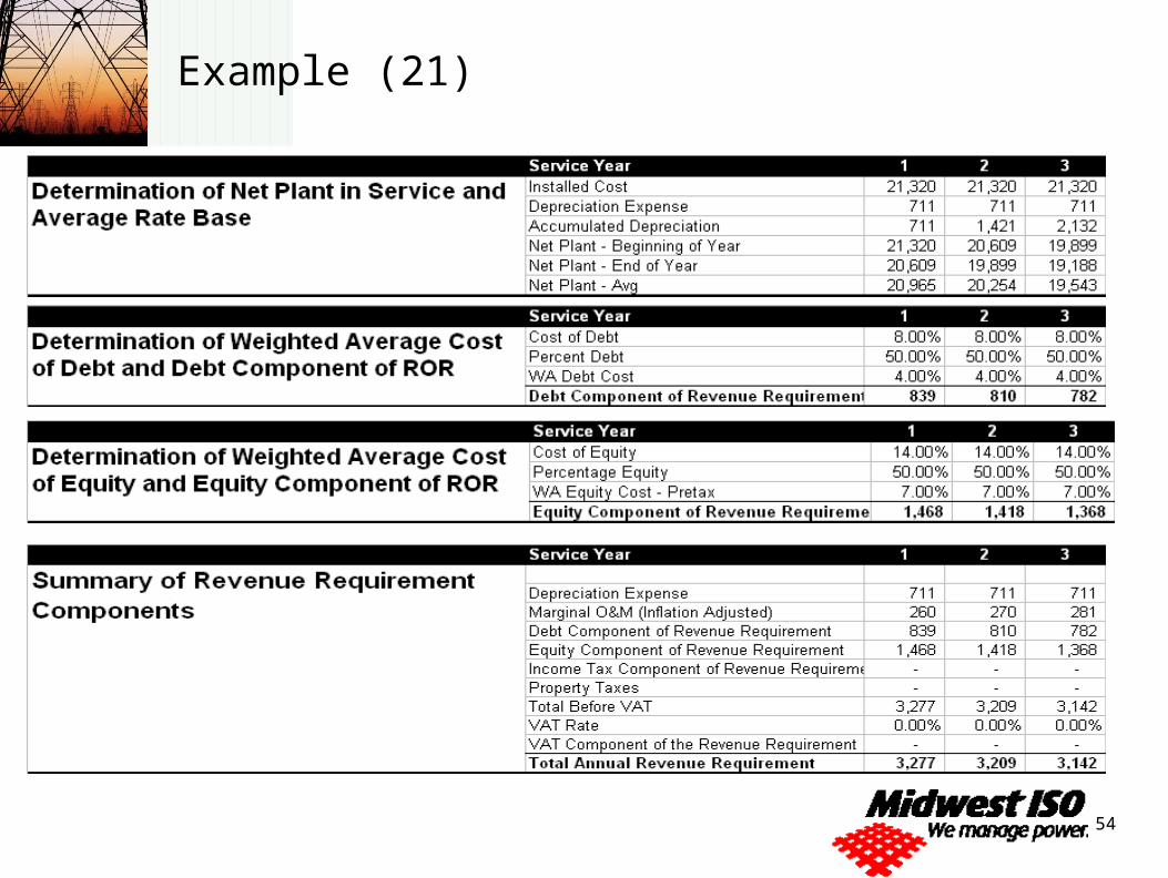
Carrying Charge Rate Calculation (19)
Revenue Requirements = (Plant in Service – Accumulated Depreciation) * WACC
+ Income Taxes
+ Property Taxes
53
Example (20)
54
Example (21)
55
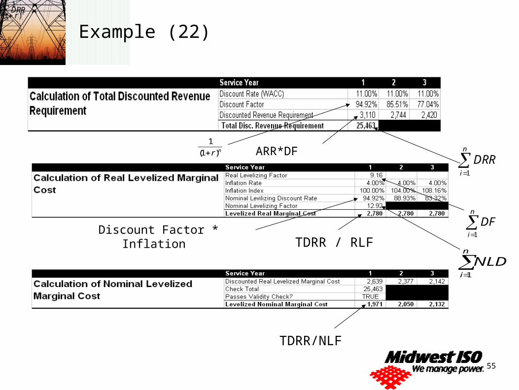
Example (22)nr)1(
1
nr)1(
1
ARR*DF
n
i
DRR1
n
i
DRR1
n
i
DF1Discount Factor * Inflation
n
i
NLDR1
TDRR / RLF
TDRR/NLF
56
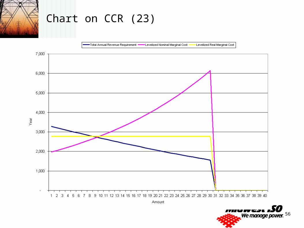
Chart on CCR (23)
57
Functional Marginal Costs (24)
Marginal cost categories are further estimated by the cost causality of each function
Generation has a capacity and energy component
Transmission has at a minimum a capacity component
Distribution has a capacity and customer component
58
Marginal Generation Capacity Costs (25)
Marginal Generation Capacity Cost is the LRMC of adding new generation to the system regardless of the price of energy from that resource.
From a system planning point of view a resource with lower energy costs (e.g., a coal plant or a hydro unit) will only be constructed if the increased value of the energy output outweighs the additional capital and fixed O&M costs over the expected life of the unit
59
Marginal Generation Costs-Capacity (26)
Definition: Marginal Generation Capacity Cost is the lowest cost alternative to provide capacity in the long-run regardless of energy price.
“Peaker Methodology”
What is the levelized cost of a simple-cycle (open-cycle) combustion turbine over its life?
The Carrying Charge Rate (CCR) calculation is then performed in order to convert the one-time installed cost and fixed O&M of the marginal generation capacity technology to an annual value
60
Marginal Generation Costs-Energy (27)
Definition: Marginal Energy Cost is the cost to provide an additional increment of energy
Methods to estimate Marginal Energy Costs include the following: Simulation: A model is used to predict the dispatch in the
region of all loads, transmission interconnections and generation resources.
Historical Data: Dispatch records of the region are analyzed in order to determine the highest cost resource in every hour for an historical period of time (e.g., a year).
Market Data: Market data from a reliable source is analyzed for an historical period of time. Future time periods (“Forward Curves”) are generally not appropriate because these include risk premiums
61
Marginal Generation Costs-Energy (28)
Since it is common for Marginal Energy Costs to vary significantly from hour to hour, typically groups of similar hours are combined in order to capture major differences in costs. These time periods are called “Costing Periods.” Examples of costing periods are Summer and Non-Summer
and On-Peak versus Off-Peak Costs.
When estimating Marginal Energy costs the effects of the wholesale markets and opportunity costs from lost transactions are taken into account.
62
Marginal Transmission Costs-Capacity (29)
Definition: The incremental cost to provide transmission service ignoring other transmission infrastructure investments such as generator interconnections
In determining marginal transmission costs, only a capacity component exists. Other components may be added in the future to capture
ancillary services pricing.
Transmission assets are constructed for a number of reasons for example: Load Growth Generation Interconnection Replacement of Existing Infrastructure.
63
Marginal Transmission Costs-Capacity (30)
Transmission investments are often made infrequently and therefore require an analysis of an extended period of time (e.g., 5-10-15 years) in order to properly estimate marginal costs.
A common way of identifying marginal transmission investments is to analyze the transmission investment budget and determine what investments are related to load growth.
Next, each investment must be restated in a constant year value matching the test year period (e.g. 2005).
64
Marginal Transmission Costs-Capacity (31)
The marginal transmission capacity costs are then calculated to determine the relationship between load growth for the period of the investments and the total load-related investments.
Methods commonly used in order to determine this relationship include: Simple arithmetic averages Regression analysis
65
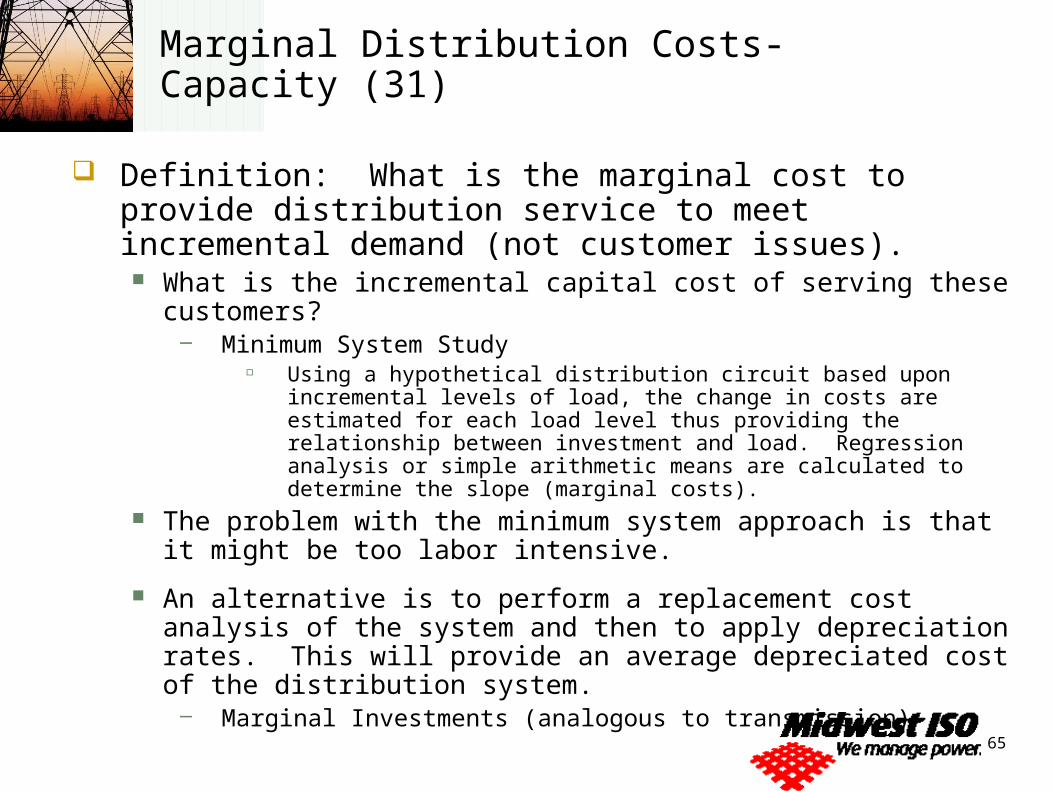
Marginal Distribution Costs-Capacity (31)
Definition: What is the marginal cost to provide distribution service to meet incremental demand (not customer issues). What is the incremental capital cost of serving these customers?
– Minimum System Study Using a hypothetical distribution circuit based upon incremental levels of load,
the change in costs are estimated for each load level thus providing the relationship between investment and load. Regression analysis or simple arithmetic means are calculated to determine the slope (marginal costs).
The problem with the minimum system approach is that it might be too labor intensive.
An alternative is to perform a replacement cost analysis of the system and then to apply depreciation rates. This will provide an average depreciated cost of the distribution system.
– Marginal Investments (analogous to transmission)
66
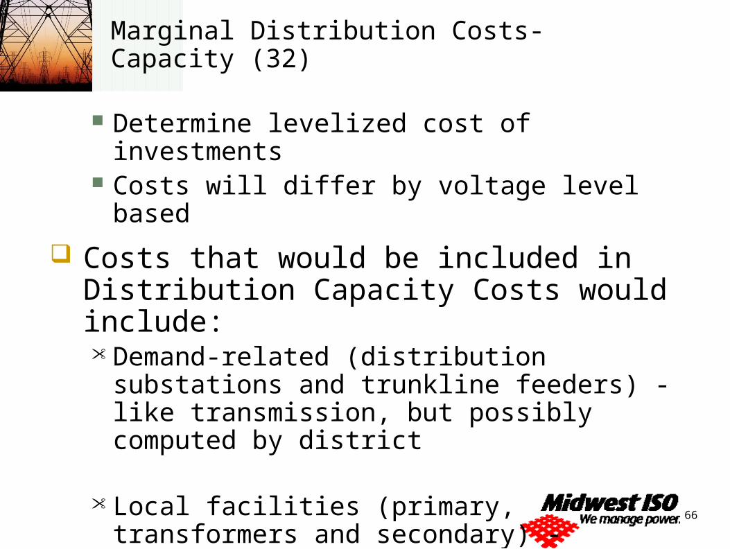
Marginal Distribution Costs-Capacity (32)
Determine levelized cost of investments Costs will differ by voltage level based
Costs that would be included in Distribution Capacity Costs would include:• Demand-related (distribution substations and
trunkline feeders) - like transmission, but possibly computed by district
• Local facilities (primary, transformers and secondary) - annualized investment per kW of design demand
67
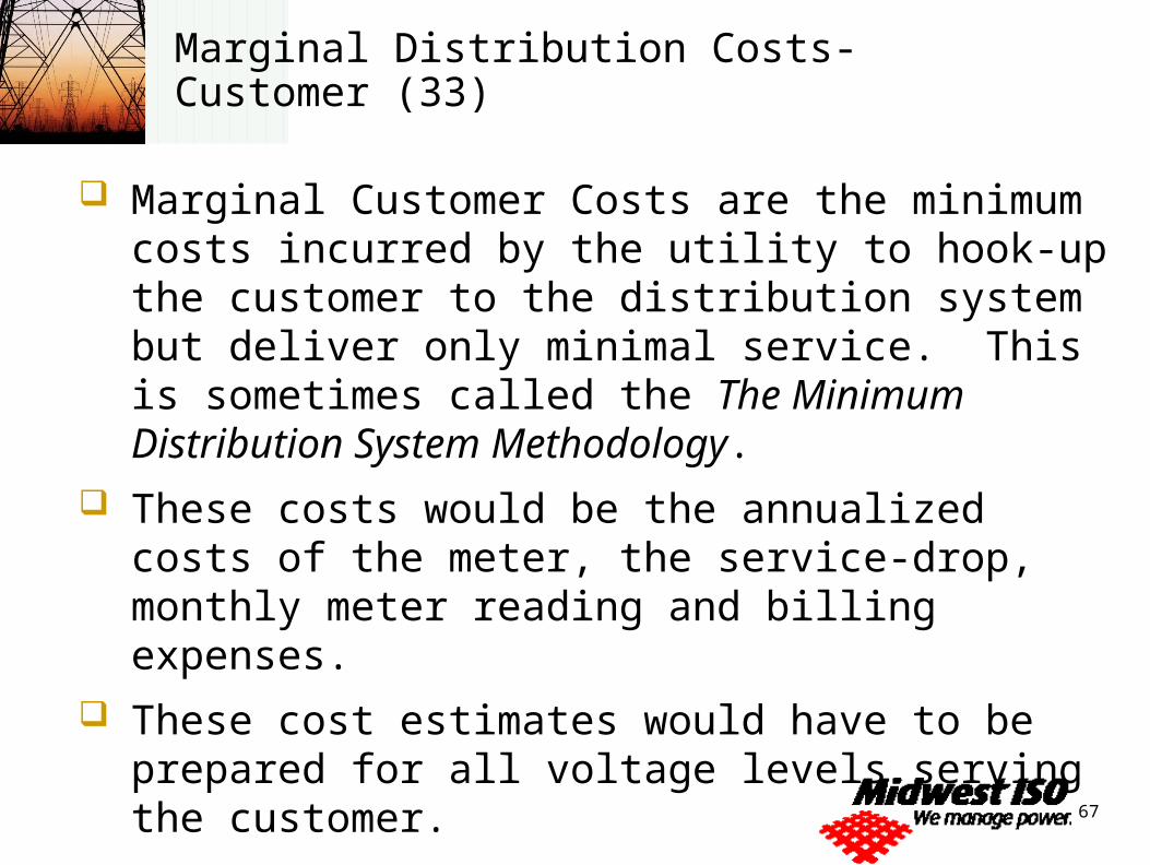
Marginal Distribution Costs-Customer (33)
Marginal Customer Costs are the minimum costs incurred by the utility to hook-up the customer to the distribution system but deliver only minimal service. This is sometimes called the The Minimum Distribution System Methodology.
These costs would be the annualized costs of the meter, the service-drop, monthly meter reading and billing expenses.
These cost estimates would have to be prepared for all voltage levels serving the customer.
68
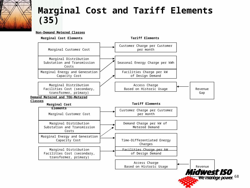
Marginal Cost and Tariff Elements (35)
Tariff Elements
Marginal Customer Cost
Marginal Distribution Substation and Transmission Costs
Marginal Energy and Generation Capacity Cost
Marginal Distribution Facilities Cost (secondary, transformer, primary)
Customer Charge per Customerper month
Seasonal Energy Charge per kWh
Revenue Gap
Marginal Customer Cost
Marginal Distribution Substation and Transmission Costs
Marginal Energy and Generation Capacity Cost
Marginal Distribution Facilities Cost (secondary, transformer, primary)
Tariff Elements
Customer Charge per Customerper month
Demand Charge per kW of Metered Demand
Time-Differentiated Energy Charges
Access ChargeBased on Historic Usage
Facilities Charge per kW of Design Demand
Revenue GapAccess Charge
Based on Historic Usage
Facilities Charge per kW of Design Demand
Marginal Cost Elements
Demand Metered and TOU-Metered Classes
Marginal Cost Elements
Non-Demand Metered Classes
Institute for Regulatory Policy Studies, Illinois State University
Allocation of Revenue Requirement
(4 Slides)
70
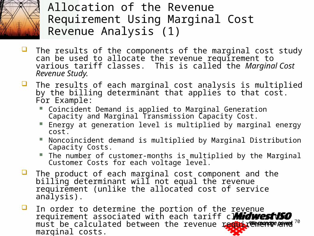
Allocation of the Revenue Requirement Using Marginal Cost Revenue Analysis (1)
The results of the components of the marginal cost study can be used to allocate the revenue requirement to various tariff classes. This is called the Marginal Cost Revenue Study.
The results of each marginal cost analysis is multiplied by the billing determinant that applies to that cost. For Example:
Coincident Demand is applied to Marginal Generation Capacity and Marginal Transmission Capacity Cost.
Energy at generation level is multiplied by marginal energy cost. Noncoincident demand is multiplied by Marginal Distribution Capacity Costs. The number of customer-months is multiplied by the Marginal Customer Costs
for each voltage level. The product of each marginal cost component and the billing determinant
will not equal the revenue requirement (unlike the allocated cost of service analysis).
In order to determine the portion of the revenue requirement associated with each tariff class a ratio must be calculated between the revenue requirement and marginal costs.
71
Allocation of the Revenue Requirement Using Marginal Cost Revenue Analysis (2)
Equal Percentage of Marginal Costs: The ratio of the total revenue requirement and the sum of marginal cost revenues is calculated and applied to each tariff class. By definition the sum of each tariff’s marginal cost responsibility will equal the revenue requirement.
72
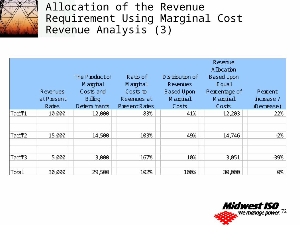
Allocation of the Revenue Requirement Using Marginal Cost Revenue Analysis (3)
Revenues at Present
Rates
The Product of Marginal
Costs and Billing
Determinants
Ratio of Marginal Costs to
Revenues at Present Rates
Distribution of Revenues
Based Upon Marginal
Costs
Revenue Allocation
Based upon Equal
Percentage of Marginal Costs
Percent Increase / (Decrease)
Tariff 1 10,000 12,000 83% 41% 12,203 22%
Tariff 2 15,000 14,500 103% 49% 14,746 -2%
Tariff 3 5,000 3,000 167% 10% 3,051 -39%
Total 30,000 29,500 102% 100% 30,000 0%
73
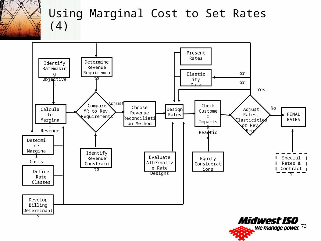
Using Marginal Cost to Set Rates (4)
DevelopBilling
Determinants
DefineRate
Classes
DetermineMarginal
Costs
IdentifyRatemakingObjectives
CalculateMarginalRevenue
EquityConsiderations
AdjustRates, Elasticities
or Rev.Req.
IdentifyRevenue
Constraints
EvaluateAlternative
Rate Designs
CompareMR to Rev.
Requirements
PresentRates
Choose Revenue Reconciliation
Method
Check Customer Impacts & Reactions
DetermineRevenue
Requirements
FINALRATES
SpecialRates &
Contracts
ElasticityData
or
or
Yes
DesignRates
NoAdjust

Institute for Regulatory Policy Studies, Illinois State University
Setting Prices
(26 Slides)
75
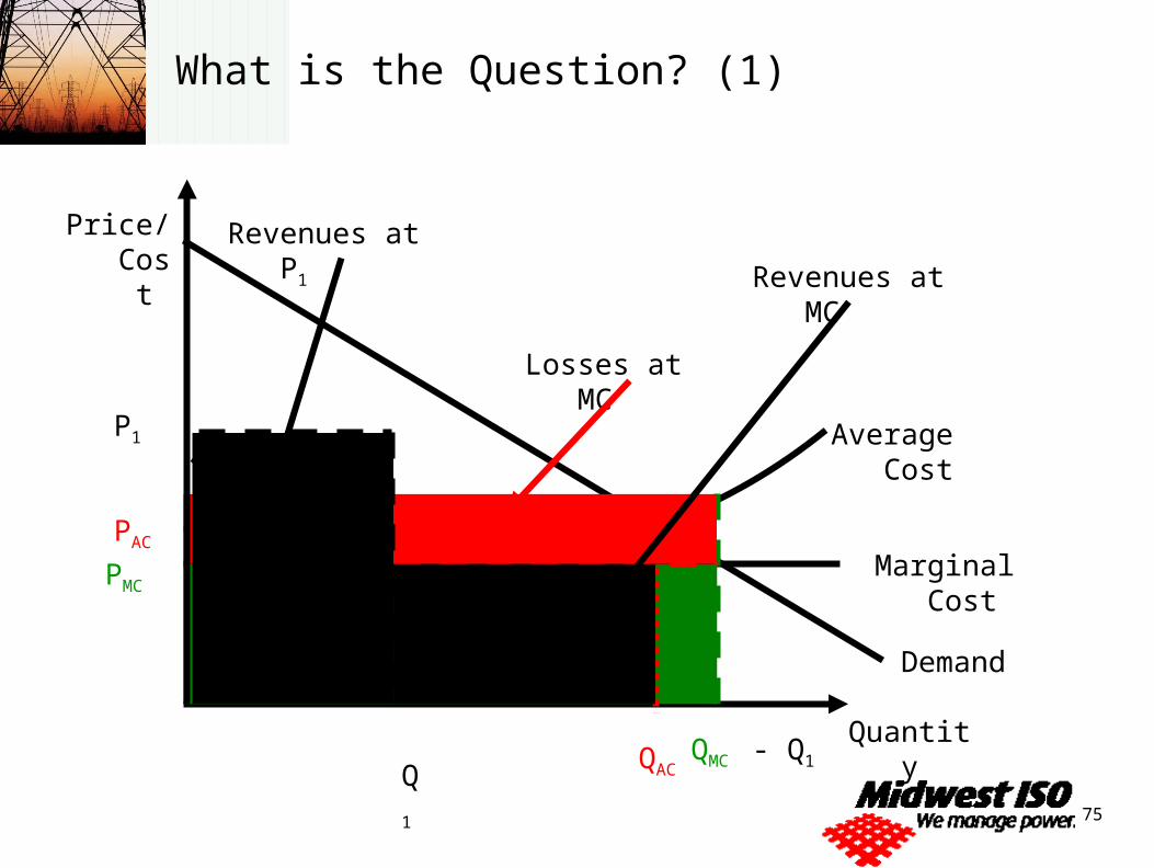
What is the Question? (1)
Price/ Cost
Quantity
Marginal Cost
Demand
Average Cost
QMC
PMC
Revenue at MC
QAC
PAC
Losses at MC
P1
Q1 - Q1
Revenues at P1
Revenues at MC
76
Types of Utility Tariffs (2)
Flat Watthour Tariffs.
Declining Watthour Tariffs.
Inverted Black Watthour Tariffs.
Hopkinson (Two-part) Tariffs.
Wright Tariffs (Load Factor Blocks).
Time of Use.
77
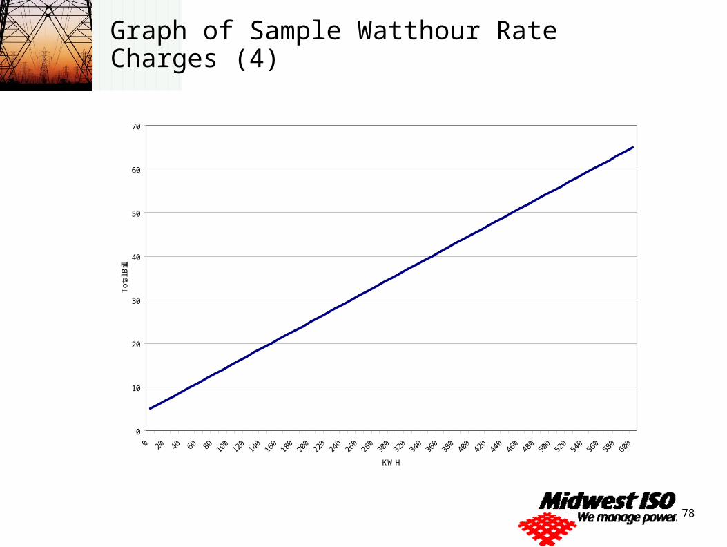
Flat Watthour Tariffs (3)
The Flat Watthour Tariff contains a energy charge that is unchanged with volume and a customer charge. All components of electric supply (with the
exception of the customer charge) are recovered through a watthour charge.
Implicit in this rate design is the assumption that the tariff class contains customers with relatively small variation in load factor, time of use and other important cost attributes.
78
Graph of Sample Watthour Rate Charges (4)
0
10
20
30
40
50
60
70
0 20 40 60 80 100
120
140
160
180
200
220
240
260
280
300
320
340
360
380
400
420
440
460
480
500
520
540
560
580
600
KWH
Tot
al B
ill
79
Advantages and Disadvantages of Watthour Tariffs (5)
Advantages Easy to bill. Easy for customers to understand. Requires simple metering technology.
Disadvantages Fails to capture differences in demand. Fails to capture difference in time-of-use. Requires that customers must be homogeneous.
80
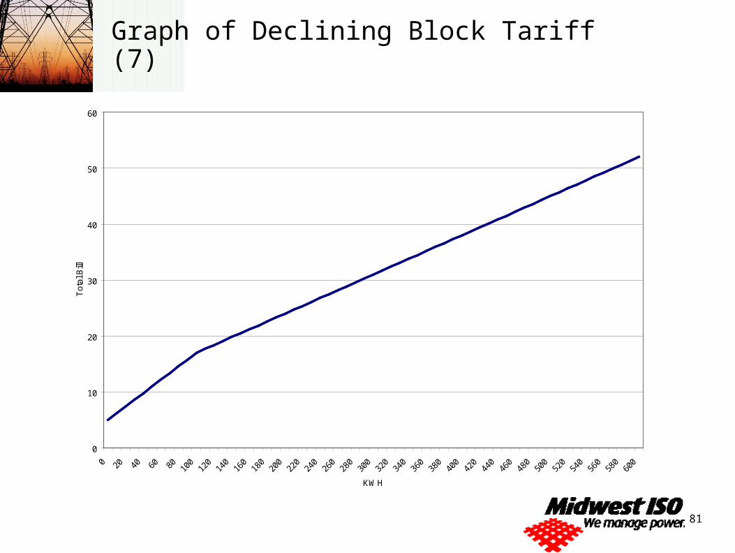
Declining Watthour Tariffs (6)
The Declining Watthour Tariff has two blocks with the a reduced watthour charge for the second block.
These tariffs are employed when the marginal cost to serve a customer is less than the average revenue requirement of the tariff.
81
Graph of Declining Block Tariff (7)
0
10
20
30
40
50
60
0 20 40 60 80 100
120
140
160
180
200
220
240
260
280
300
320
340
360
380
400
420
440
460
480
500
520
540
560
580
600
KWH
Tot
al B
ill
82
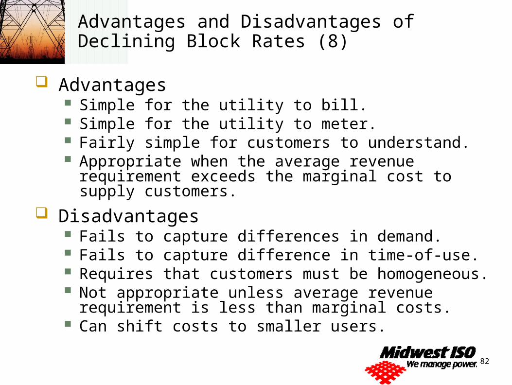
Advantages and Disadvantages of Declining Block Rates (8)
Advantages Simple for the utility to bill. Simple for the utility to meter. Fairly simple for customers to understand. Appropriate when the average revenue requirement exceeds
the marginal cost to supply customers.
Disadvantages Fails to capture differences in demand. Fails to capture difference in time-of-use. Requires that customers must be homogeneous. Not appropriate unless average revenue requirement is less
than marginal costs. Can shift costs to smaller users.
83
Increasing Block Watthour Tariffs (9)
The Increasing Block Tariff is the opposite of the Declining Block Tariff – the last block of usage is billed at a higher charge.
This type of rate design is appropriate when the average revenue requirement is less than the marginal cost to serve customers.
84
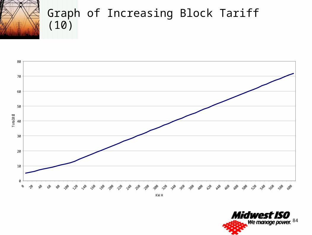
Graph of Increasing Block Tariff (10)
0
10
20
30
40
50
60
70
80
0 20 40 60 80 100
120
140
160
180
200
220
240
260
280
300
320
340
360
380
400
420
440
460
480
500
520
540
560
580
600
KWH
Tot
al B
ill
85
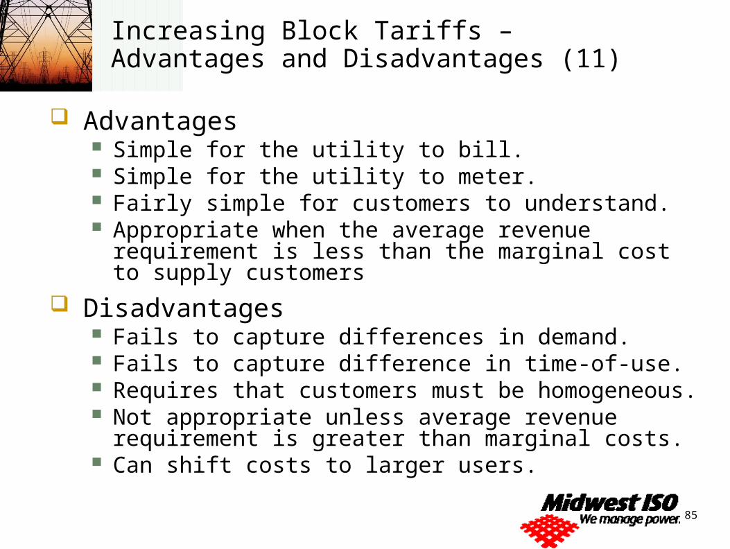
Increasing Block Tariffs – Advantages and Disadvantages (11)
Advantages Simple for the utility to bill. Simple for the utility to meter. Fairly simple for customers to understand. Appropriate when the average revenue requirement is less
than the marginal cost to supply customers
Disadvantages Fails to capture differences in demand. Fails to capture difference in time-of-use. Requires that customers must be homogeneous. Not appropriate unless average revenue requirement is
greater than marginal costs. Can shift costs to larger users.
86
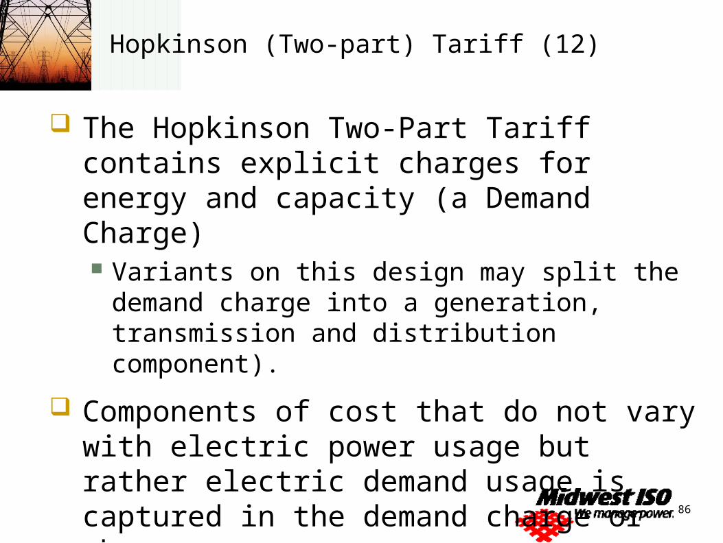
Hopkinson (Two-part) Tariff (12)
The Hopkinson Two-Part Tariff contains explicit charges for energy and capacity (a Demand Charge) Variants on this design may split the demand
charge into a generation, transmission and distribution component).
Components of cost that do not vary with electric power usage but rather electric demand usage is captured in the demand charge or charges.
87
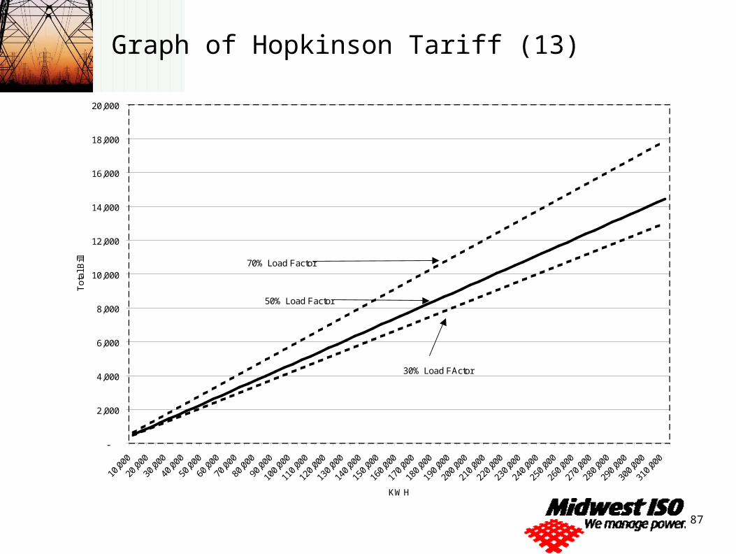
Graph of Hopkinson Tariff (13)
-
2,000
4,000
6,000
8,000
10,000
12,000
14,000
16,000
18,000
20,000
10,0
00
20,0
00
30,0
00
40,0
00
50,0
00
60,0
00
70,0
00
80,0
00
90,0
00
100,
000
110,
000
120,
000
130,
000
140,
000
150,
000
160,
000
170,
000
180,
000
190,
000
200,
000
210,
000
220,
000
230,
000
240,
000
250,
000
260,
000
270,
000
280,
000
290,
000
300,
000
310,
000
KWH
Tot
al B
ill 70% Load Factor
50% Load Factor
30% Load FActor
88
Advantages and Disadvantages of Hopkinson Tariffs (14)
Advantages Captures the differences in load factor form customer to
customer. Is generally understood by larger customers. Provides explicit price signal to customers for both energy
and capacity.
Disadvantages Requires more costly meters. The metering investment
must be balanced with the benefits of implementing the tariff. Requires more effort to bill.
89
Demand Charge Ratchet Mechanisms (15)
Demand Charge Ratchets are implemented on Hopkinson Tariffs for cost components which are established by the customer’s highest demand in a series of billing periods (e.g., each year).
Distribution charges often are good candidates for a demand ratchet. The cost of the radial portion of the distribution
system is established by the highest demand for an annual period even if the customer does not use that demand each month.
90
Advantages and Disadvantages of Demand Ratchets (16)
Advantages Provides the customers with a better price signal
regarding component costs. Provides an additional mechanism for the
unbundling of tariffs.
Disadvantages. More difficult for the customer to understand. More difficult to bill.
91
Time of Use Tariffs (17)
The Time of Use tariff differentiates between the cost of the energy charge component of the tariff between high costs and lower cost period.
Time of Use tariffs can either be watthour tariffs or Hopkinson tariffs.
92
Advantages and Disadvantages of Time of Use Tariffs (18)
Advantages. Provides a better price signal to the customer. Moves the tariff to better matching of costs and
revenues.
Disadvantages. Requires more costly metering equipment. If more difficult to understand.
93
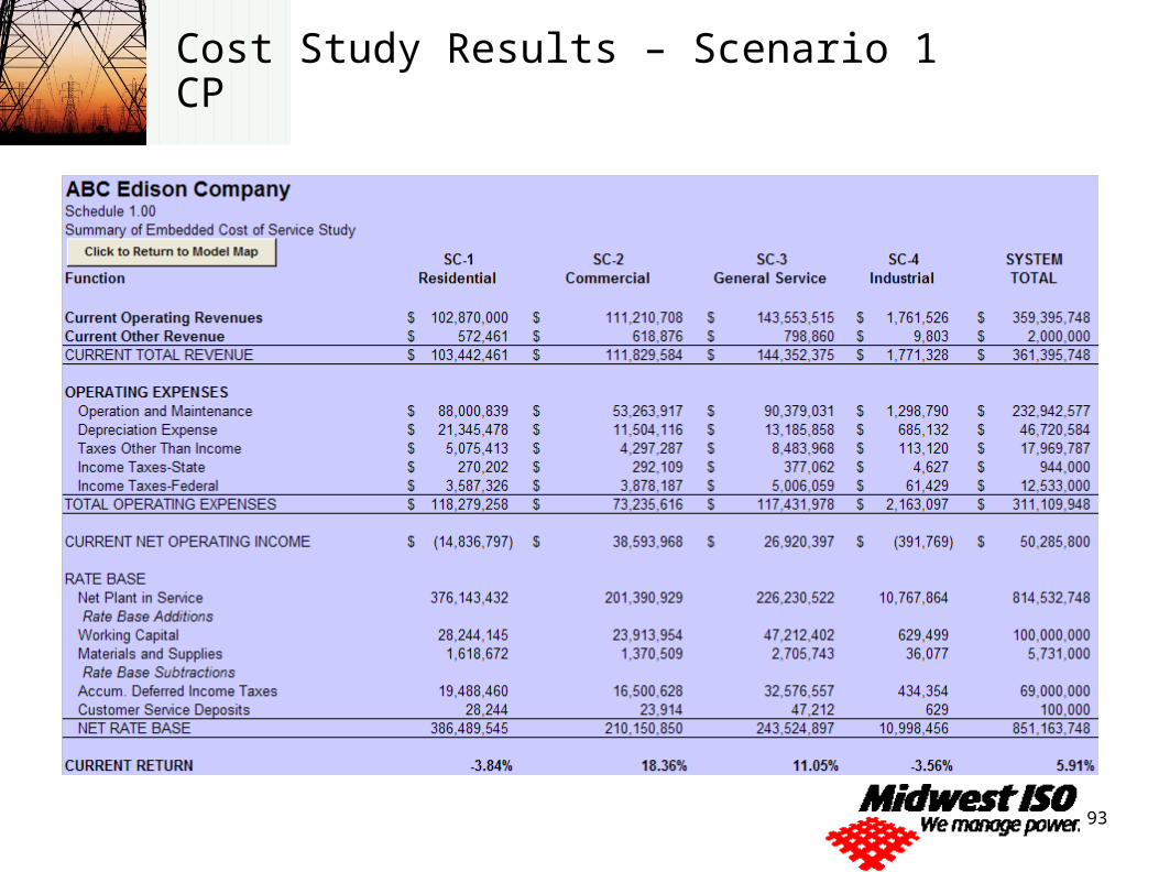
Cost Study Results – Scenario 1 CP
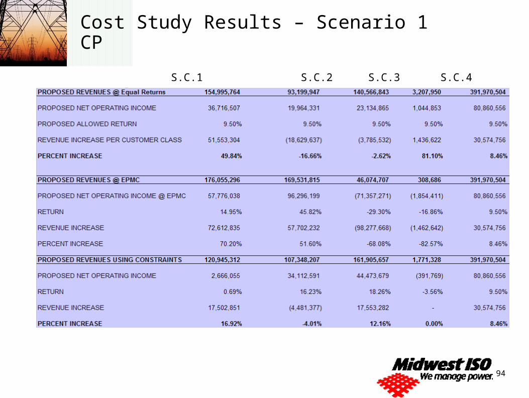
94
Cost Study Results – Scenario 1 CP
S.C.1 S.C.2 S.C.3 S.C.4 Total
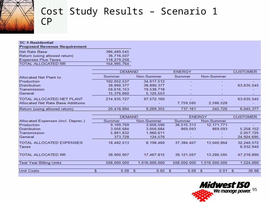
95
Cost Study Results – Scenario 1 CP
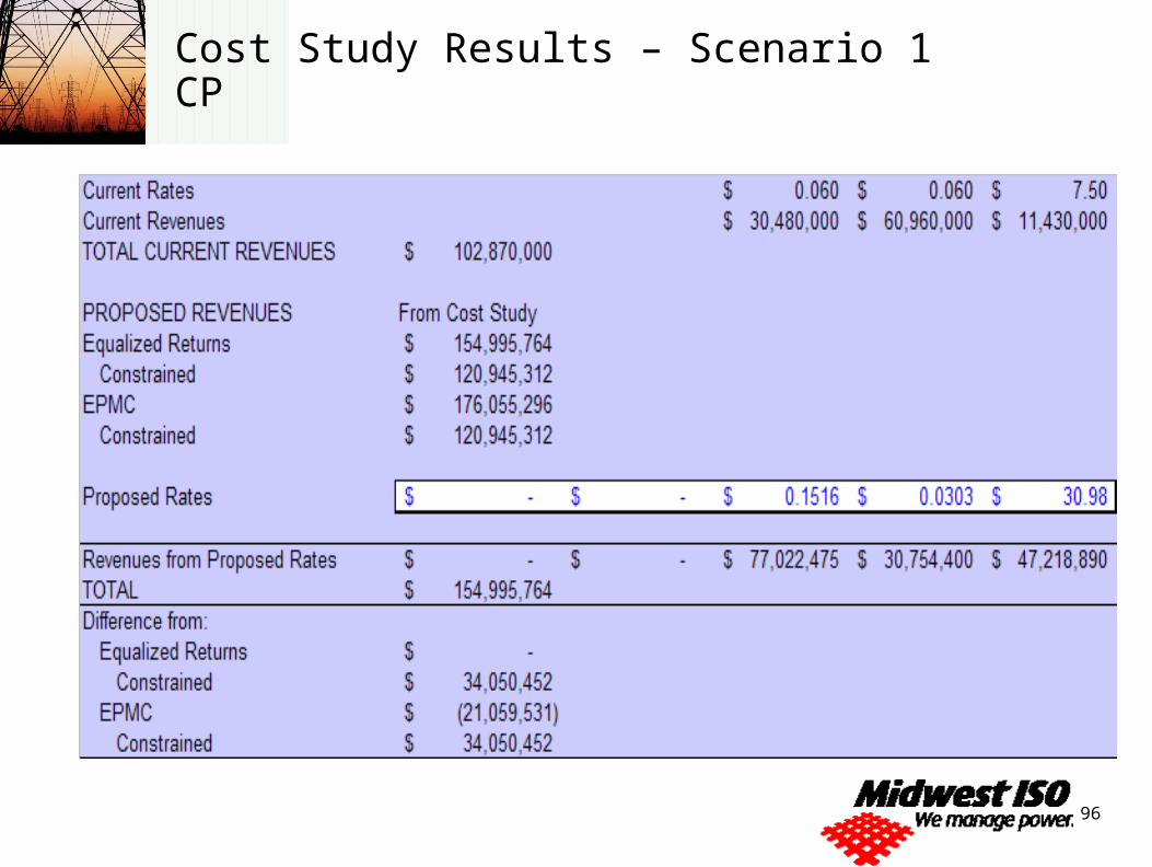
96
Cost Study Results – Scenario 1 CP
97
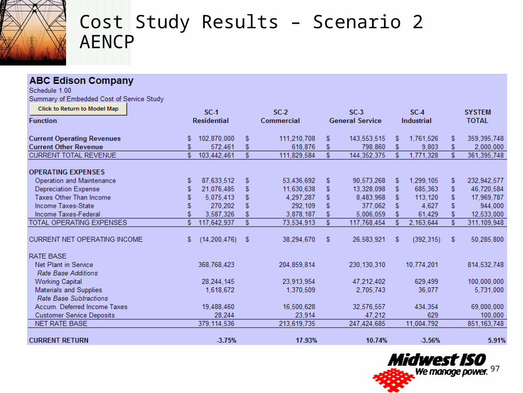
Cost Study Results – Scenario 2 AENCP
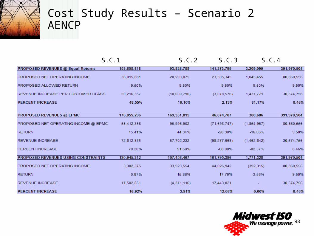
98
Cost Study Results – Scenario 2 AENCP
S.C.1 S.C.2 S.C.3 S.C.4 Total
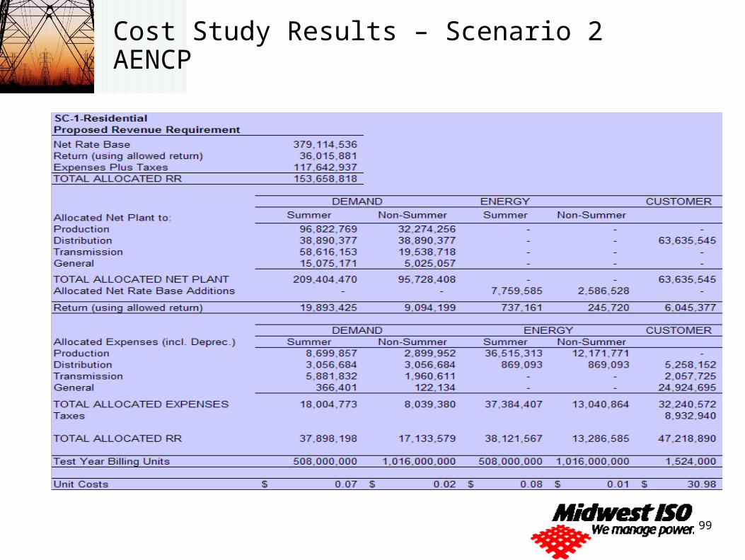
99
Cost Study Results – Scenario 2 AENCP

100
Cost Study Results – Scenario 2 AENCP
Related Documents