Institut für Höhere Studien (IHS), Wien Institute for Advanced Studies, Vienna Reihe Ökonomie / Economics Series No. 42 Unanticipated Money Thomas F. Cooley, Gary D. Hansen

Welcome message from author
This document is posted to help you gain knowledge. Please leave a comment to let me know what you think about it! Share it to your friends and learn new things together.
Transcript

Institut für Höhere Studien (IHS), Wien Institute for Advanced Studies, Vienna Reihe Ökonomie / Economics Series No. 42
Unanticipated Money
Thomas F. Cooley, Gary D. Hansen
Unanticipated Money
Thomas F. Cooley, Gary D. Hansen
Reihe Ökonomie / Economics Series No. 42
March 1997
Thomas F. Cooley Department of Economics University of Rochester Harkness Hall Rochester, NY 14627-0156, U.S.A. Phone: ++1/716/275-8380 e-mail: [email protected] Gary D. Hansen Department of Economics University of California, Los Angeles 2263 Bunche Hall Box 951477 Los Angeles, CA 90095-1477, U.S.A. Phone: ++1/310/825-3847 Fax: ++1/310/825-9528 e-mail: [email protected]
Institut für Höhere Studien (IHS), Wien Institute for Advanced Studies, Vienna

The Institute for Advanced Studies in Vienna is an independent center of postgraduate training and research in the social sciences. The Economics Series presents research done at the Economics Department of the Institute for Advanced Studies. Department members, guests, visitors, and other researchers are invited to contribute and to submit manuscripts to the editors. All papers are subjected to an internal refereeing process.
Editorial Main Editor: Robert M. Kunst (Econometrics) Associate Editors: Walter Fisher (Macroeconomics) Arno Riedl (Microeconomics)

Abstract
The role of unanticipated changes in money growth for aggregate fluctuations is reexamined
using the methods of quantitative equilibrium business cycle theory. A stochastic growth
model with money is constructed that has the feature, following Lucas (1972, 1975), that
production and trade take place in spatially separated markets (islands). Individuals must infer
changes in the aggregate price level from observing local relative prices. This causes
individuals to react to changes in the average price level, due to unanticipated changes in the
aggregate money supply, as though they were changes in market specific relative prices.
We show that this mechanism can lead to quantitatively large fluctuations in real economic
activity. The statistical properties of these fluctuations, however, are quite different from the
properties of fluctuations observed in the U.S. economy.
Keywords Business cycles, monetary policy, aggregate fluctuations, real business cycles
JEL-Classifications E32, E52

Comments
This paper has been prepared for a conference on the “Dynamic Effects of Monetary Policy,” held at the Federal Reserve Bank of Cleveland in November 1996. We acknowledge helpful comments on previous versions from David Altig, Satyajit Chatterjee, Russell Cooper, Paul Gomme, and Tryphon Kollintzas.


I H S — Cooley, Hansen / Unanticipated Money — 1
1. Introduction
In Lucas (1972), an economy is described in which unanticipated increases in the money
growth rate leads to increases in the level of employment and output. This idea was extended
in Lucas (1975) to a neoclassical growth economy with capital accumulation and modern
equilibrium business cycle theory was born. The results obtained in that paper, however, were
only qualitative in nature. Later, Kydland and Prescott (1982) described a methodology for
obtaining quantitative results from equilibrium business cycle models, and these techniques
are now standard in the theoretical literature on aggregate fluctuations. However, the model
that Kydland and Prescott studied is one in which the impulses that lead to business cycles
are shocks to technology rather than changes in the growth rate of money. The purpose of the
current paper is to reexamine the idea of Lucas (1972, 1975) using the methods of quantitative
equilibrium business cycle theory. Our goal is to use Lucas’s model to study the importance
of monetary shocks for fluctuations in real variables in the same sense that the real business
cycle literature studies the importance of technology shocks.
This is not the first attempt to study the quantitative implications of the Lucas story. Kydland
and Prescott (1982), Kydland (1989) and Cooley & Hansen (1995) all describe economies
which attempt to capture the central feature of the islands model using a technology shock
that is observed with noise. Agents face a signal extraction problem, as they do in the Lucas
model, and the noise is only informally interpreted as resulting from monetary policy. Those
studies found that noise shocks have only a small effect on output fluctuations. In this paper
we are explicit about the role of money and the role of island-specific shocks. Our findings
suggest that the conclusions of those earlier papers were misleading.
The economy we study is a close relative of the cash-in-advance economy studied in Cooley
and Hansen (1995). In that model, changes in the growth rate of money affect real variables
only to the extent that they signal changes in the inflation tax. That is, increases in the growth
rate of money lead agents to expect higher inflation in the future. In response to this, agents
substitute away from activities that involve the use of cash in favor of activities that do not
require cash. The model studied in this paper introduces an additional monetary non-
neutrality: agents confuse changes in the economy wide price level with changes in a market
specific relative price. This is because agents are only able to observe the market price; they
can not observe (or accurately infer) the economy wide average price level. This leads perfectly
rational agents to confuse money shocks with market specific demand shocks and respond to
the former as though they were the latter.
In the next section, we describe the details of this model. In the third section, we discuss our
findings. Some brief concluding comments are provided in section 4.
2 — Cooley, Hansen / Unanticipated Money — I H S
2. The Model Economy
In this section we describe three model economies. The first is a real business cycle model
with money introduced by imposing a cash-in-advance constraint. The model is similar to the
one studied in Cooley and Hansen (1995) except that agents live in spatially separated
markets, or islands, and newly printed money is distributed unequally across these islands.
The second economy, discussed in section 2.2, is a linear quadratic approximation of the first
economy. Finally, in section 2.3, we incorporate informational asymmetries of the sort
described in the introduction to the linear-quadratic economy. Computational tractability is our
reason for forming a linear-quadratic approximate economy before introducing informational
asymmetries. We perform quantitative experiments with the latter economy in section 3.
2.1. A Cash-in-Advance Economy with Spatially Separated Markets
We consider a world consisting of a large number of spatially separated markets (islands) with
measure 1 households per island with identical preferences and initial endowments. Each
household is composed of a shopper-worker pair, as in Lucas and Stokey (1987). These
agents, who live forever, choose consumption and work effort to maximize expected discounted
lifetime utility,
E c c htt t t
t
β α α γ β α[ log ( ) log ], .1 20
1 0 1 0 1+ − − < < < <=
∞
∑ and (1)
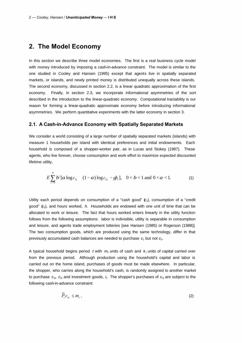
Utility each period depends on consumption of a “cash good” (c1), consumption of a “credit
good” (c2), and hours worked, h. Households are endowed with one unit of time that can be
allocated to work or leisure. The fact that hours worked enters linearly in the utility function
follows from the following assumptions: labor is indivisible, utility is separable in consumption
and leisure, and agents trade employment lotteries [see Hansen (1985) or Rogerson (1988)].
The two consumption goods, which are produced using the same technology, differ in that
previously accumulated cash balances are needed to purchase c1 but not c2.
A typical household begins period t with mt units of cash and k t units of capital carried over
from the previous period. Although production using the household’s capital and labor is
carried out on the home island, purchases of goods must be made elsewhere. In particular,
the shopper, who carries along the household’s cash, is randomly assigned to another market
to purchase c1t, c2t and investment goods, it. The shopper’s purchases of c1t are subject to the
following cash-in-advance constraint:
~P c mt t t1 ≤ , (2)
I H S — Cooley, Hansen / Unanticipated Money — 3
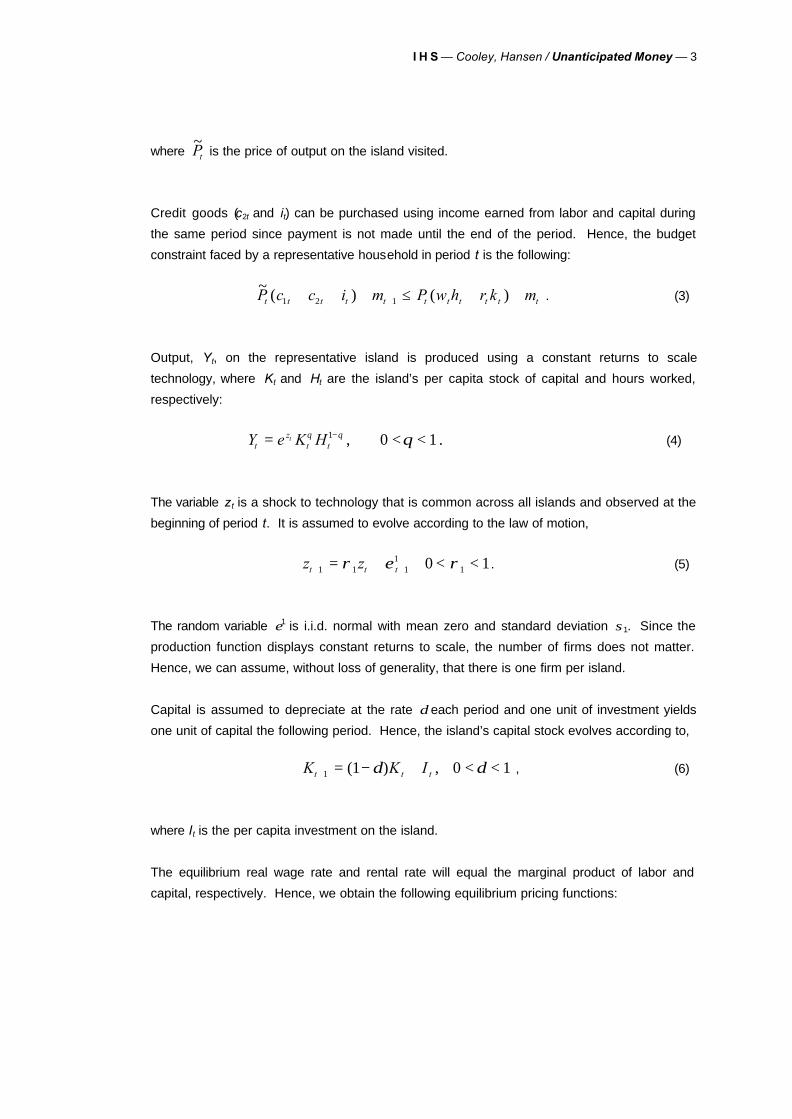
where ~Pt is the price of output on the island visited.
Credit goods (c2t and it) can be purchased using income earned from labor and capital during
the same period since payment is not made until the end of the period. Hence, the budget
constraint faced by a representative household in period t is the following:
~ ( ) ( )P c c i m P w h r k mt t t t t t t t t t t1 2 1+ + + ≤ + ++ . (3)
Output, Yt, on the representative island is produced using a constant returns to scale
technology, where Kt and Ht are the island’s per capita stock of capital and hours worked,
respectively:
Y e K Htz
t tt= < <−θ θ θ1 0 1, . (4)
The variable zt is a shock to technology that is common across all islands and observed at the
beginning of period t. It is assumed to evolve according to the law of motion,
z zt t t+ += + < <1 1 11
10 1ρ ε ρ . (5)
The random variable ε1 is i.i.d. normal with mean zero and standard deviation σ1. Since the
production function displays constant returns to scale, the number of firms does not matter.
Hence, we can assume, without loss of generality, that there is one firm per island.
Capital is assumed to depreciate at the rate δ each period and one unit of investment yields
one unit of capital the following period. Hence, the island’s capital stock evolves according to,
K K It t t+ = − + < <1 1 0 1( ) ,δ δ , (6)
where It is the per capita investment on the island.
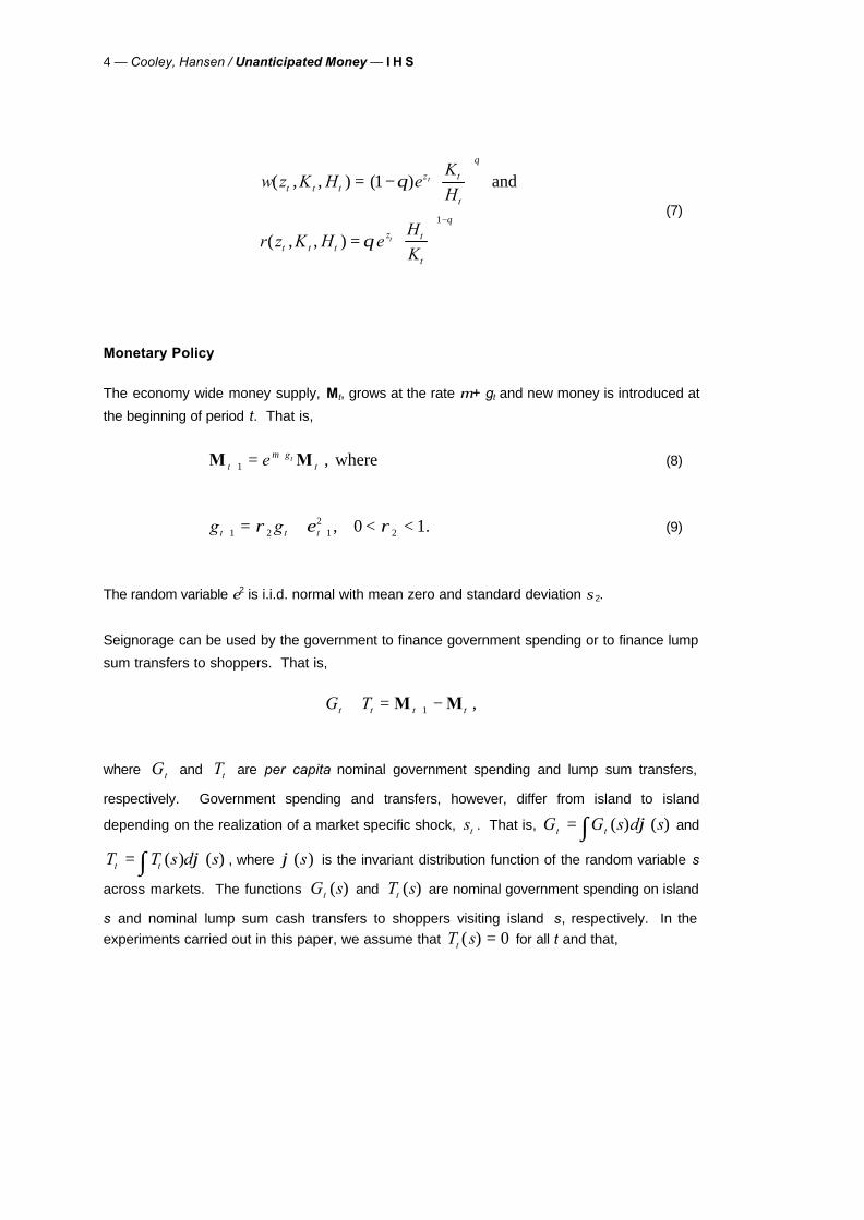
The equilibrium real wage rate and rental rate will equal the marginal product of labor and
capital, respectively. Hence, we obtain the following equilibrium pricing functions:
4 — Cooley, Hansen / Unanticipated Money — I H S
w z K H eKH
r z K H eHK
t t tz t
t
t t tz t
t
t
t
( , , ) ( )
( , , )
= −
=
−
1
1
θ
θ
θ
θ
and
(7)
Monetary Policy
The economy wide money supply, Mt, grows at the rate µ + gt and new money is introduced at
the beginning of period t. That is,
M Mtg
te t+
+=1µ , where (8)
g gt t t+ += + < <1 2 12
20 1ρ ε ρ, . (9)
The random variable ε2 is i.i.d. normal with mean zero and standard deviation σ2.
Seignorage can be used by the government to finance government spending or to finance lump
sum transfers to shoppers. That is,
G Tt t t t+ = −+M M1 ,
where Gt and Tt are per capita nominal government spending and lump sum transfers,
respectively. Government spending and transfers, however, differ from island to island
depending on the realization of a market specific shock, st . That is, G G s d st t= ∫ ( ) ( )ϕ and
T T s d st t= ∫ ( ) ( )ϕ , where ϕ( )s is the invariant distribution function of the random variable s
across markets. The functions G st ( ) and T st ( ) are nominal government spending on island
s and nominal lump sum cash transfers to shoppers visiting island s, respectively. In the experiments carried out in this paper, we assume that T st ( ) = 0 for all t and that,
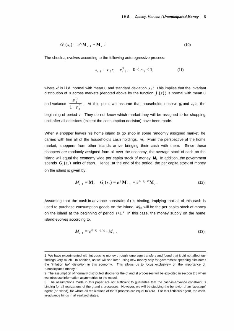
I H S — Cooley, Hansen / Unanticipated Money — 5
G s et ts
t tt( ) = −+M M1 .1 (10)
The shock st evolves according to the following autoregressive process:
s st t t+ += + < <1 3 13
30 1ρ ε ρ, , (11)
where ε3 is i.i.d. normal with mean 0 and standard deviation σ3.2 This implies that the invariant distribution of s across markets (denoted above by the function ϕ( )s ) is normal with mean 0
and variance σ
ρ32
321−
. At this point we assume that households observe gt and st at the
beginning of period t. They do not know which market they will be assigned to for shopping
until after all decisions (except the consumption decision) have been made.
When a shopper leaves his home island to go shop in some randomly assigned market, he
carries with him all of the household’s cash holdings, mt. From the perspective of the home
market, shoppers from other islands arrive bringing their cash with them. Since these
shoppers are randomly assigned from all over the economy, the average stock of cash on the
island will equal the economy wide per capita stock of money, Mt. In addition, the government spends G st t( ) units of cash. Hence, at the end of the period, the per capita stock of money
on the island is given by,
M G s e et t t ts
ts g
tt t t
+ ++ += + = =1 1M M M( ) µ . (12)
Assuming that the cash-in-advance constraint (1) is binding, implying that all of this cash is
used to purchase consumption goods on the island, Mt+1 will be the per capita stock of money
on the island at the beginning of period t+1.3 In this case, the money supply on the home
island evolves according to,
M e Mtg s s
tt t t
++ + −= −
11µ . (13)
1 We have experimented with introducing money through lump sum transfers and found that it did not affect our findings very much. In addition, as we will see later, using new money only for government spending eliminates the “inflation tax” distortion in this economy. This allows us to focus exclusively on the importance of “unanticipated money.” 2 The assumption of normally distributed shocks for the gt and st processes will be exploited in section 2.3 when we introduce information asymmetries to the model. 3 The assumptions made in this paper are not sufficient to guarantee that the cash-in-advance constraint is binding for all realizations of the g and s processes. However, we will be studying the behavior of an “average” agent (or island), for whom all realizations of the s process are equal to zero. For this fictitious agent, the cash-in-advance binds in all realized states.
6 — Cooley, Hansen / Unanticipated Money — I H S
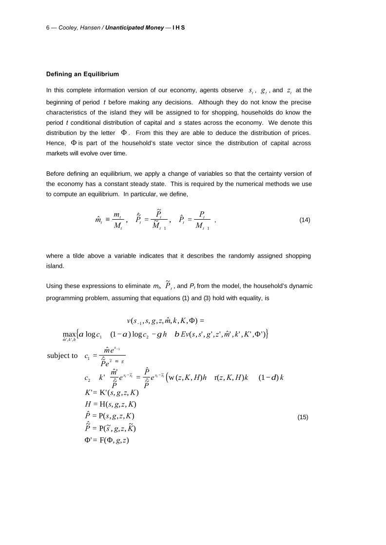
Defining an Equilibrium
In this complete information version of our economy, agents observe st , g t , and zt at the
beginning of period t before making any decisions. Although they do not know the precise
characteristics of the island they will be assigned to for shopping, households do know the
period t conditional distribution of capital and s states across the economy. We denote this
distribution by the letter Φ . From this they are able to deduce the distribution of prices.
Hence, Φ is part of the household’s state vector since the distribution of capital across
markets will evolve over time.
Before defining an equilibrium, we apply a change of variables so that the certainty version of
the economy has a constant steady state. This is required by the numerical methods we use
to compute an equilibrium. In particular, we define,
$ , ~$~
~ , $mmM
PP
MP
PMt
t
tt
t
tt
t
t
≡ = =+ +1 1
, (14)
where a tilde above a variable indicates that it describes the randomly assigned shopping
island.
Using these expressions to eliminate mt, ~P t , and Pt from the model, the household’s dynamic
programming problem, assuming that equations (1) and (3) hold with equality, is
{ }
( )
v s s g z m k K
c c h Ev s s g z m k K
cme
Pe
c km
Pe
P
Pe z K H h z K H k k
m k h
s
s g
s s s st t t t
( , , , , $ , , , )
max log ( ) log ( , ', ' , ' , $ ' , ' , ' , ')
$~$
'$ '~$
$
~$ w ( , , ) r( , , ) ( )
$ ', ',
~
~ ~
−
+ +
− −
=
+ − − +
=
+ + = + + −
−
1
1 2
1
2
1
1
1
Φ
Φα α γ β
δ
µsubject to
K s g z K
H s g z K
P s g z K
P s g z K
g z
' K'( , , , )
H( , , , )$ P( , , , )~$ P(~, , , ~)
' F( , , )
===
==Φ Φ
(15)
I H S — Cooley, Hansen / Unanticipated Money — 7
The maximization is also subject to the laws of motion for the exogenous shocks, given by
equations (4) (8), and (10). In addition, the functions w and r are defined in equation (6). Note that last period’s realization of the market specific shock, s−1 , affects the current return but
does not enter the agent’s decision rules. This is because the value of s−1 only affects the
value of cash-good consumption. Given that (1) holds with equality, c1 is determined by
decisions made in the previous period rather than the current period. In addition, c2 is
determined so that (3) holds with equality. Hence, since c1 and c2 are chosen residually,
their realization will depend on the characteristics of the randomly assigned shopping island, ~ ~s K and , in addition to the set of state variables.
The last five constraints in (14) represent the household’s perceptions of how market variables,
which are outside the control of the household, depend on the state of the market. The first of
these determines the market specific capital stock for next period, and the second determines
per capita hours worked in the market. These perceptions are necessary for agents to
compute expected future wage and rental rates [see equation (6)]. The third and fourth
equations represent the household’s knowledge of how prices are determined, both on the
home island and on the randomly assigned shopping island. Since islands are identical
expect for the realized values of s and K, the functional form of these two pricing functions are
identical. The last equation in (14) gives the law of motion for the joint distribution of ~ ~s K and
as a function of the economy wide state variables, z and g.
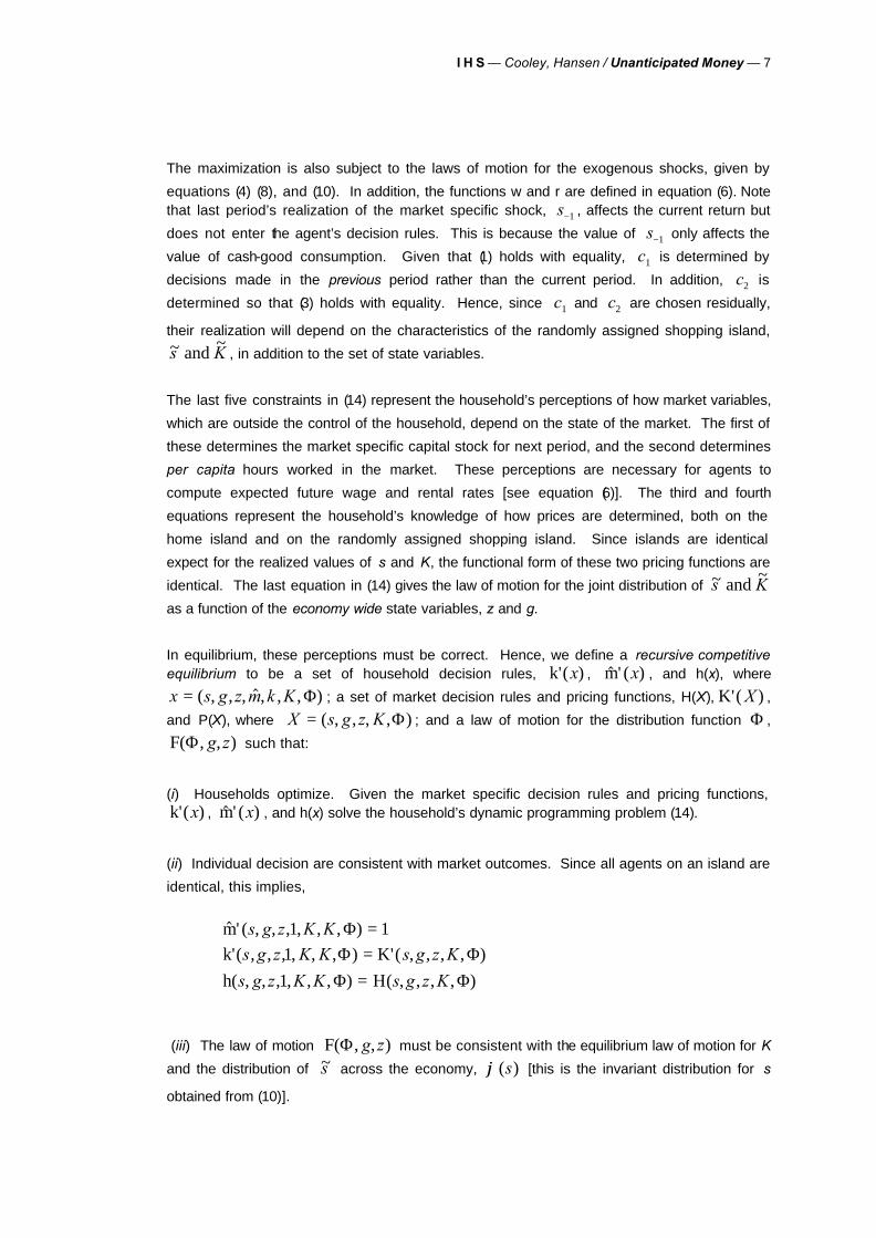
In equilibrium, these perceptions must be correct. Hence, we define a recursive competitive equilibrium to be a set of household decision rules, k'( )x , $m' ( )x , and h(x), where
x s g z m k K= ( , , , $ , , , )Φ ; a set of market decision rules and pricing functions, H(X), K'( )X ,
and P(X), where X s g z K= ( , , , , )Φ ; and a law of motion for the distribution function Φ ,
F( , , )Φ g z such that:
(i) Households optimize. Given the market specific decision rules and pricing functions, k'( )x , $m' ( )x , and h(x) solve the household’s dynamic programming problem (14).
(ii) Individual decision are consistent with market outcomes. Since all agents on an island are
identical, this implies,
$m' ( , , , , , , )k'( , , , , , , ) K'( , , , , )
h( , , , , , , ) H( , , , , )
s g z K Ks g z K K s g z K
s g z K K s g z K
1 11
1
ΦΦ ΦΦ Φ
==
=
(iii) The law of motion F( , , )Φ g z must be consistent with the equilibrium law of motion for K
and the distribution of ~s across the economy, ϕ( )s [this is the invariant distribution for s
obtained from (10)].
8 — Cooley, Hansen / Unanticipated Money — I H S
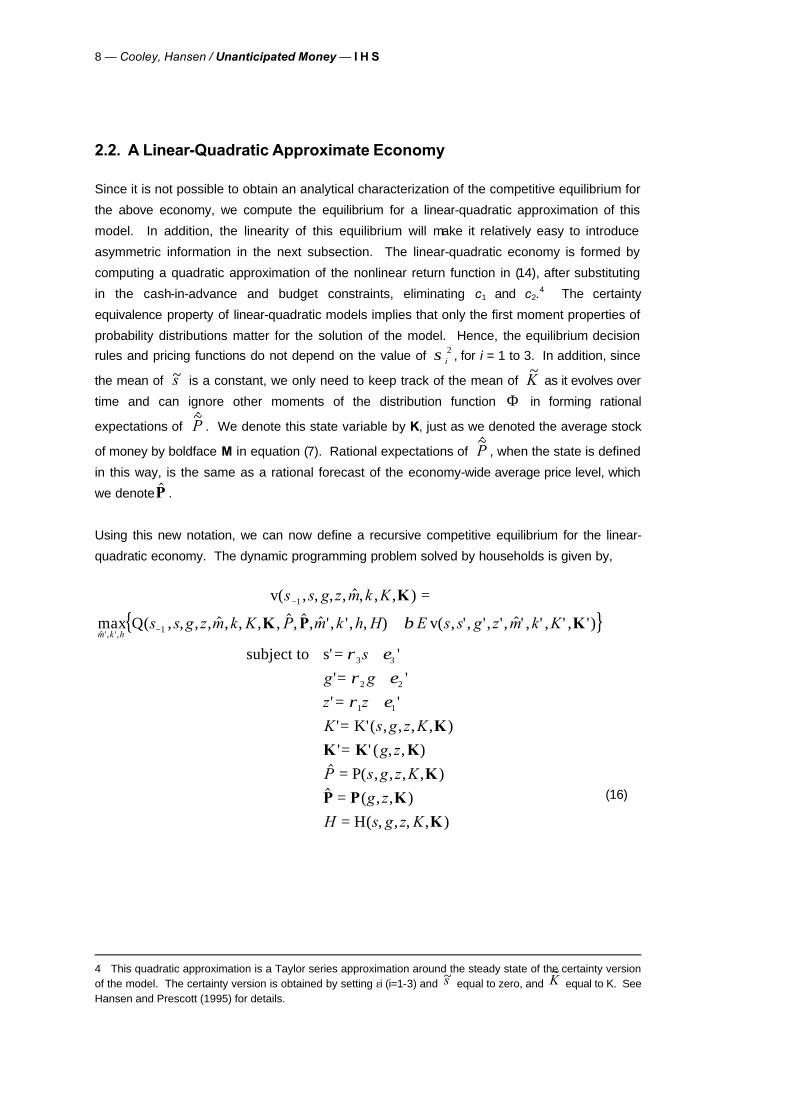
2.2. A Linear-Quadratic Approximate Economy
Since it is not possible to obtain an analytical characterization of the competitive equilibrium for
the above economy, we compute the equilibrium for a linear-quadratic approximation of this
model. In addition, the linearity of this equilibrium will make it relatively easy to introduce
asymmetric information in the next subsection. The linear-quadratic economy is formed by
computing a quadratic approximation of the nonlinear return function in (14), after substituting
in the cash-in-advance and budget constraints, eliminating c1 and c2.4 The certainty
equivalence property of linear-quadratic models implies that only the first moment properties of
probability distributions matter for the solution of the model. Hence, the equilibrium decision rules and pricing functions do not depend on the value of σi
2 , for i = 1 to 3. In addition, since
the mean of ~s is a constant, we only need to keep track of the mean of ~K as it evolves over
time and can ignore other moments of the distribution function Φ in forming rational
expectations of ~$P . We denote this state variable by K, just as we denoted the average stock
of money by boldface M in equation (7). Rational expectations of ~$P , when the state is defined
in this way, is the same as a rational forecast of the economy-wide average price level, which
we denote $P .
Using this new notation, we can now define a recursive competitive equilibrium for the linear-
quadratic economy. The dynamic programming problem solved by households is given by,
{ }v( , , , , $ , , , )
max Q( , , , , $ , , , , $ , $ , $ ' , ' , , ) v( , ', ' , ' , $ ' , ' , ' , ')
'
' '
' '
' K'( , , , , )
' ' ( , , )
$ ', ',
s s g z m k K
s s g z m k K P m k h H E s s g z m k K
s
g g
z z
K s g z K
g z
m k h
−
−
=
+
+= += +==
1
1
3
2 2
1 1
K
K P K
K
K K K
β
ρ ερ ερ ε
subject to s'= 3
$ P( , , , , )$ ( , , )
H( , , , , )
P s g z K
g z
H s g z K
===
K
P P K
K
(16)
4 This quadratic approximation is a Taylor series approximation around the steady state of the certainty version of the model. The certainty version is obtained by setting εi (i=1-3) and
~s equal to zero, and ~K equal to K. See
Hansen and Prescott (1995) for details.
I H S — Cooley, Hansen / Unanticipated Money — 9
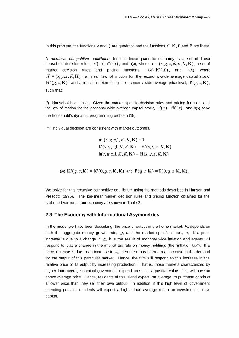
In this problem, the functions v and Q are quadratic and the functions K′, K′, P and P are linear.
A recursive competitive equilibrium for this linear-quadratic economy is a set of linear household decision rules, k'( )x , $m' ( )x , and h(x), where x s g z m k K= ( , , , $ , , , )K ; a set of
market decision rules and pricing functions, H(X), K'( )X , and P(X), where
X s g z K= ( , , , , )K ; a linear law of motion for the economy-wide average capital stock,
K K'( , , )g z ; and a function determining the economy-wide average price level, P K( , , )g z ,
such that:
(i) Households optimize. Given the market specific decision rules and pricing function, and the law of motion for the economy-wide average capital stock, k'( )x , $m' ( )x , and h(x) solve
the household’s dynamic programming problem (15).
(ii) Individual decision are consistent with market outcomes,
$m' ( , , , , , , )k'( , , , , , , ) K'( , , , , )
h( , , , , , , ) H( , , , , )
s g z K Ks g z K K s g z K
s g z K K s g z K
1 11
1
KK K
K K
==
=
(iii) K K K K'( , , ) K'( , , , , )g z g z= 0 and P K K K( , , ) P( , , , , )g z g z= 0 .
We solve for this recursive competitive equilibrium using the methods described in Hansen and
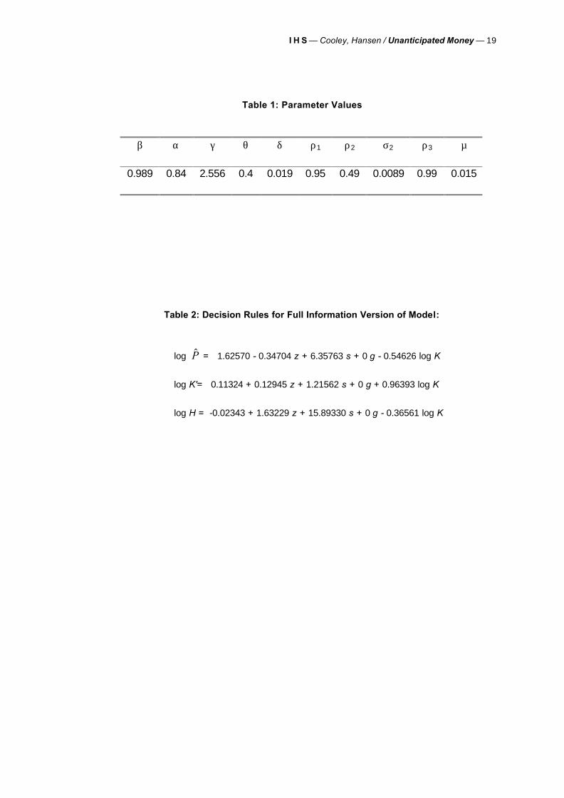
Prescott (1995). The log-linear market decision rules and pricing function obtained for the
calibrated version of our economy are shown in Table 2.
2.3 The Economy with Informational Asymmetries
In the model we have been describing, the price of output in the home market, Pt, depends on
both the aggregate money growth rate, gt, and the market specific shock, st. If a price
increase is due to a change in gt, it is the result of economy wide inflation and agents will
respond to it as a change in the implicit tax rate on money holdings (the “inflation tax”). If a
price increase is due to an increase in st, then there has been a real increase in the demand
for the output of this particular market. Hence, the firm will respond to this increase in the
relative price of its output by increasing production. That is, those markets characterized by
higher than average nominal government expenditures, i.e. a positive value of st, will have an
above average price. Hence, residents of this island expect, on average, to purchase goods at
a lower price than they sell their own output. In addition, if this high level of government
spending persists, residents will expect a higher than average return on investment in new
capital.
10 — Cooley, Hansen / Unanticipated Money — I H S
We now introduce informational asymmetries to the linear-quadratic economy defined in the
previous subsection. The critical feature of Lucas’s (1972, 1975) model, which we now
incorporate, is that agents can only observe, and hence make decisions contingent on, the
price of output in their own market. They cannot infer the average price level of the economy
as a whole.5 The implication of our informational assumptions is that households are not able
to observe the two shocks, gt and st, separately.6 This introduces the possibility that agents
may confuse changes in these two shocks and respond to a change in the economy wide
average price level (resulting from a change in gt) as though it were at least partly a change in
the relative price of output in the home market (a change in st).
To be more specific, at the beginning of period t, the information set a particular agent uses to
form expectations of gt and st, is I P P j tj j0 = <{ ,~
, } .7 Before any decisions are made, the
agent observes Pt , the price of output on his own island. Hence, his information set is now
I P P j tj j1 1= ≤−{ ,~
, } . After observing this, agents form conditional expectations of s and g,
s E s Ite
t= ( | )1 and g E g Ite
t= ( | )1 . Agents make decisions based on these conditional
expectations rather than on direct observations of these two shocks. Hence, the market
decision rules and pricing function defined in the previous subsection become H( , , , $ , , , )s g z m k Ke e eK , K'( , , , $ , , , )s g z m k Ke e eK , and P( , , , $ , , , )s g z m k Ke e eK ,
where K K Ke e eg z' ' ( , , )= describes how agents’ conditional expectations of the economy-
wide average stock of capital evolve.8
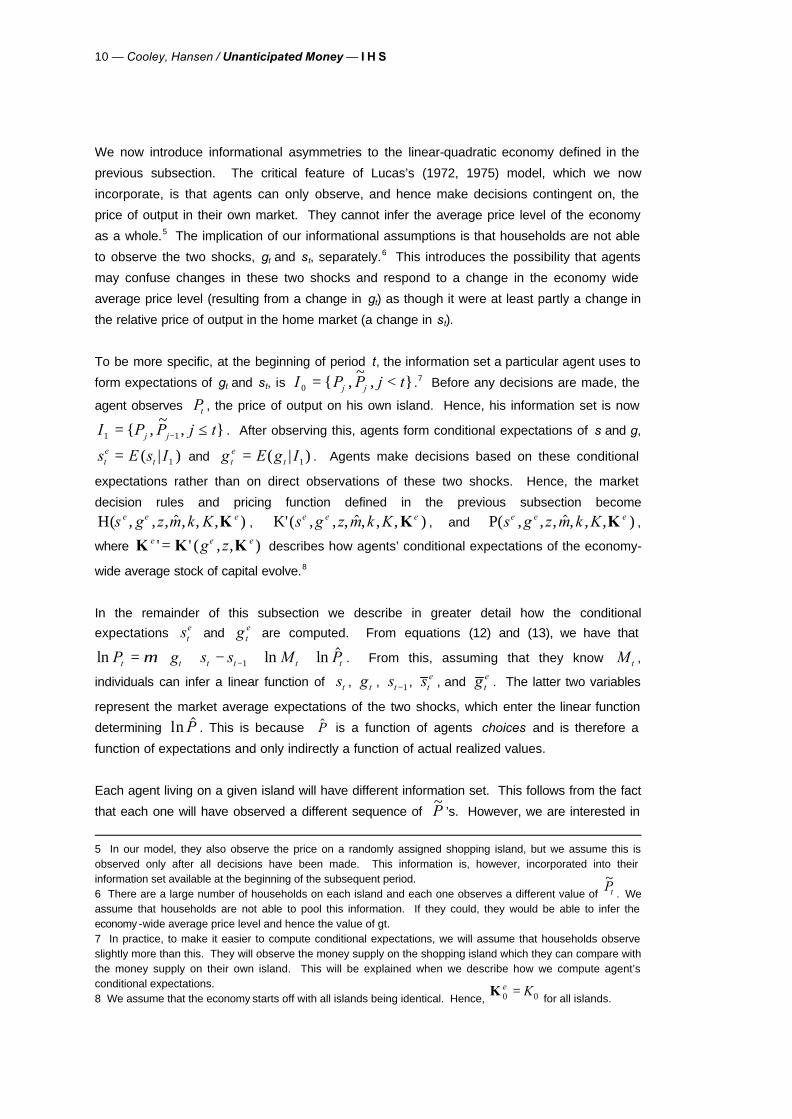
In the remainder of this subsection we describe in greater detail how the conditional expectations st
e and g te are computed. From equations (12) and (13), we have that
ln ln ln $P g s s M Pt t t t t t= + + − + +−µ 1 . From this, assuming that they know M t ,
individuals can infer a linear function of st , g t , st −1 , ste , and g t
e . The latter two variables
represent the market average expectations of the two shocks, which enter the linear function
determining ln $P . This is because $P is a function of agents choices and is therefore a
function of expectations and only indirectly a function of actual realized values.
Each agent living on a given island will have different information set. This follows from the fact
that each one will have observed a different sequence of ~P ’s. However, we are interested in
5 In our model, they also observe the price on a randomly assigned shopping island, but we assume this is observed only after all decisions have been made. This information is, however, incorporated into their information set available at the beginning of the subsequent period. 6 There are a large number of households on each island and each one observes a different value of
~Pt . We assume that households are not able to pool this information. If they could, they would be able to infer the economy -wide average price level and hence the value of gt. 7 In practice, to make it easier to compute conditional expectations, we will assume that households observe slightly more than this. They will observe the money supply on the shopping island which they can compare with the money supply on their own island. This will be explained when we describe how we compute agent’s conditional expectations. 8 We assume that the economy starts off with all islands being identical. Hence,
K 0 0e K=
for all islands.
I H S — Cooley, Hansen / Unanticipated Money — 11
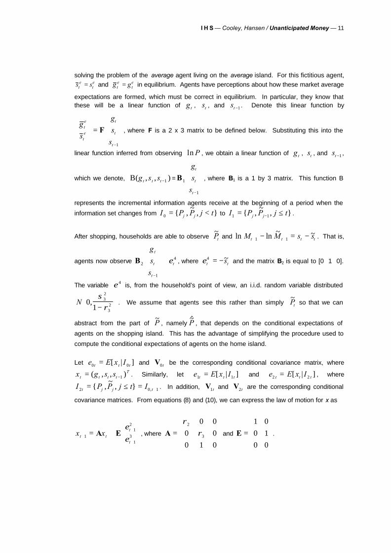
solving the problem of the average agent living on the average island. For this fictitious agent, s st
ete= and g gt
ete= in equilibrium. Agents have perceptions about how these market average
expectations are formed, which must be correct in equilibrium. In particular, they know that these will be a linear function of g t , st , and st −1 . Denote this linear function by
g
s
g
s
s
te
te
t
t
t
=
−
F
1
, where F is a 2 x 3 matrix to be defined below. Substituting this into the
linear function inferred from observing ln P , we obtain a linear function of g t , st , and st −1 ,
which we denote, B( , , )g s st t t −1 = B1
1
g
s
s
t
t
t −
, where B1 is a 1 by 3 matrix. This function B
represents the incremental information agents receive at the beginning of a period when the
information set changes from I P P j tj j0 = <{ ,~
, } to I P P j tj j1 1= ≤−{ ,~
, } .
After shopping, households are able to observe ~Pt and ln ln ~ ~M M s st t t t+ +− = −1 1 . That is,
agents now observe B2
1
4
g
s
s
t
t
t
t
−
+ε , where εt ts4 = −~ and the matrix B2 is equal to [0 1 0].
The variable ε4 is, from the household’s point of view, an i.i.d. random variable distributed
N 01
32
32,
σρ−
. We assume that agents see this rather than simply
~Pt so that we can
abstract from the part of ~P , namely
~$P , that depends on the conditional expectations of
agents on the shopping island. This has the advantage of simplifying the procedure used to
compute the conditional expectations of agents on the home island.
Let e E x It t t0 0= [ | ] and V0t be the corresponding conditional covariance matrix, where
x g s st t t tT= −( , , )1 . Similarly, let e E x It t t1 1= [ | ] and e E x It t t2 2= [ | ] , where
I P P j t It j j t2 0 1= ≤ = +{ ,~
, } , . In addition, V1t and V2t are the corresponding conditional
covariance matrices. From equations (8) and (10), we can express the law of motion for x as
x xt tt
t+
+
+
= +
1
12
13A E
εε
, where A =
ρρ
2
3
0 0
0 0
0 1 0
and E =
1 0
0 1
0 0
.
12 — Cooley, Hansen / Unanticipated Money — I H S
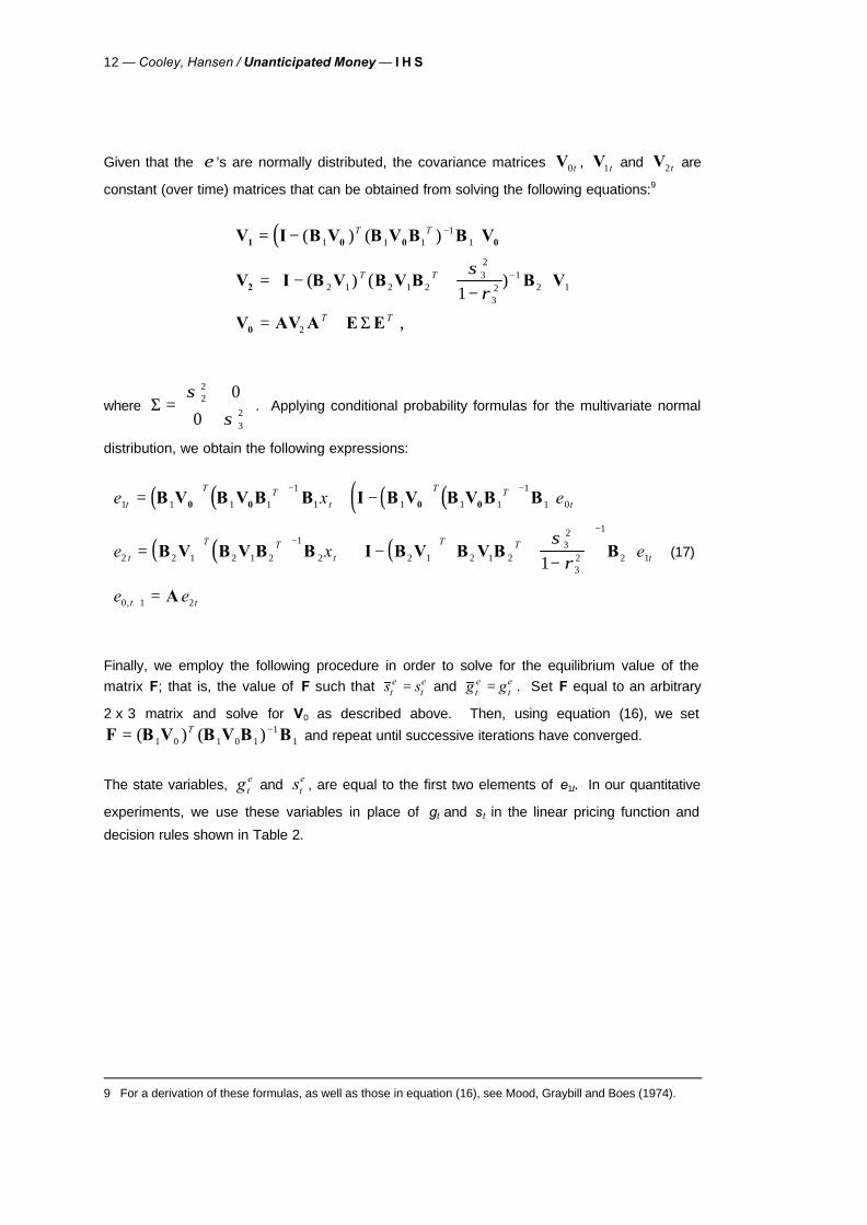
Given that the ε ’s are normally distributed, the covariance matrices V0t , V1t and V2t are
constant (over time) matrices that can be obtained from solving the following equations:9
( )V I B V B V B B V
V I B V B V B B V
V AV A E E
1 0 0 0
2
0
= −
= − +−
= +
−
−
( ) ( )
( ) ( )
,
1 1 11
1
2 1 2 1 232
32
12 1
2
1
T T
T T
T T
σρ
Σ
where Σ =
σσ
22
32
0
0. Applying conditional probability formulas for the multivariate normal
distribution, we obtain the following expressions:
( ) ( ) ( ) ( )( )( ) ( ) ( )
e x e
e x e
e e
t
T Tt
T Tt
t
T Tt
T Tt
t t
1 1 1 1
1
1 1 1 1
1
1 0
2 2 1 2 1 2
1
2 2 1 2 1 232
32
1
2 1
0 1 2
1
= + −
= + − +−
=
− −
−−
+
B V B V B B I B V B V B B
B V B V B B I B V B V B B
A
0 0 0 0
σρ
,
(17)
Finally, we employ the following procedure in order to solve for the equilibrium value of the matrix F; that is, the value of F such that s st
ete= and g gt
ete= . Set F equal to an arbitrary
2 x 3 matrix and solve for V0 as described above. Then, using equation (16), we set F B V B V B B= −( ) ( )1 0 1 0 1
11
T and repeat until successive iterations have converged.
The state variables, g te and st
e , are equal to the first two elements of e1t. In our quantitative
experiments, we use these variables in place of gt and st in the linear pricing function and
decision rules shown in Table 2.
9 For a derivation of these formulas, as well as those in equation (16), see Mood, Graybill and Boes (1974).
I H S — Cooley, Hansen / Unanticipated Money — 13
3. Quantitative Results
In this section we do three things. First, we describe the calibration of the model. Second, we
consider the impulse response of the endogenous variables of the model to a one-standard
deviation shock to the money growth rate. For comparison, we also consider the response of
the same set of variables to a technology shock. Finally, we present results from three
simulation experiments designed to assess the importance of money growth shocks for
business cycles. In particular, these experiments enable us to compare the business cycle
properties of our model economy with the same properties of postwar U.S. data.
3.1 Calibration
Given that the model studied here is very similar to the cash-in-advance economy presented in
Cooley and Hansen (1995), we follow the calibration procedure employed in that paper
whenever appropriate. In particular, we chose β, γ, θ, and δ so that the steady state capital-
output ratio, investment-output ratio, labor income share, and time spent participating in the
labor market are equal to the average of these values computed from U.S. data.10 Similarly, we
employ the same value for α as in our previous paper. In particular, we chose α based on
information from a survey of consumer transactions administered by the Federal Reserve Board
in 1984 and 1986, which lead us to choose α = .84. According to this survey, 84 percent of
consumer transactions are made with cash, if we define cash to be currency, checks, and
money orders.
The parameters of the money supply process (µ, ρ2, and σ2 in equation 8) were assigned
values based on estimates from a first order autoregression of the growth rate of M1 (again,
see our previous paper for details). The autoregressive parameter of the technology shock
process (ρ1) was chosen to match the stochastic properties of the Solow residual. In our
experiments, we consider alternative values for the standard deviation, σ1.
We do not attempt to calibrate, at least in the usual sense, the parameters of the idiosyncratic
shock process, s. Given that we do not have much information from actual economies that
can be used to calibrate this stochastic process, we chose to calibrate in a way that gives the
economy with money growth shocks the best chance of accounting for the business cycle
facts. In particular, the autoregressive parameter of this process (ρ3 in equation 10) was
chosen so as to make the response of the model to aggregate money growth shocks as
persistent as possible. By setting ρ3 close to 1, agents are driven to produce more and
accumulate capital in response to a positive value of ε3 since they expect the good times to persist for a long time. This lead us to choose ρ3 = .99.11 As with σ1 , we experiment with
10 See Cooley and Prescott (1995) for details. 11 We chose not to allow s to follow a random walk since this would imply that the standard deviation of
~s would be infinite. This would mean that agents would learn nothing from observing the price on their assigned shopping island.
14 — Cooley, Hansen / Unanticipated Money — I H S
alternative values for σ3 . The exact values assigned to each of the parameters are given in
Table 1.
3.2 Impulse Response Functions
In computing the impulse response functions shown in Figures 1 - 4, we set the standard deviation of innovations to the technology shock process,σ1 , equal to 0.00685. This value was
chosen because it is the number that enables our model with only technology shocks to
explain one hundred percent of the variance in output observed in U.S. time series. Similarly,
the standard deviation of innovations to the idiosyncratic process was chosen so that money growth shocks explain all of the variation in output. This lead us to set σ2 00048= . .
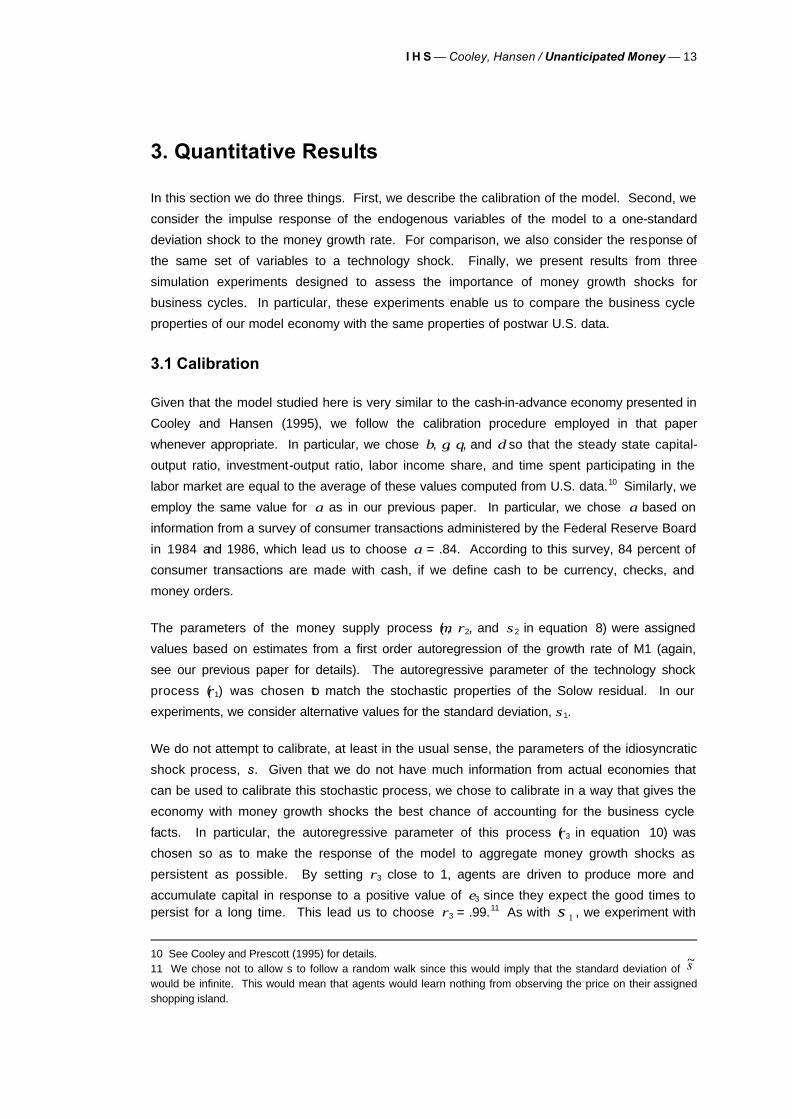
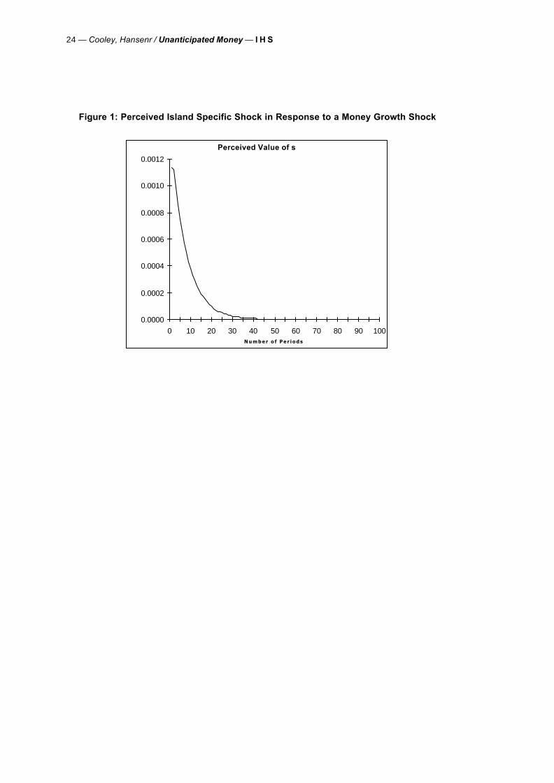
In Figure 1 we show the response of se to a one standard deviation shock to aggregate
money growth. This shows that it takes agents a large number of periods to learn that the
true value of s is zero. The half life of the misperceived increase in s is about 7 or 8 quarters.
Hence, the fact that agents never directly observe g and s leads to a fair amount of persistence
in this model.
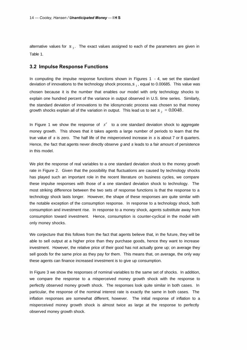
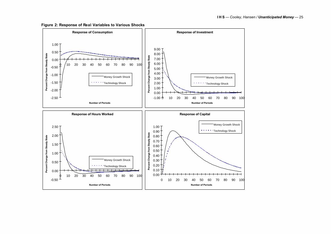
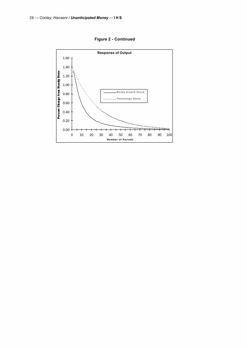
We plot the response of real variables to a one standard deviation shock to the money growth
rate in Figure 2. Given that the possibility that fluctuations are caused by technology shocks
has played such an important role in the recent literature on business cycles, we compare
these impulse responses with those of a one standard deviation shock to technology. The
most striking difference between the two sets of response functions is that the response to a
technology shock lasts longer. However, the shape of these responses are quite similar with
the notable exception of the consumption response. In response to a technology shock, both
consumption and investment rise. In response to a money shock, agents substitute away from
consumption toward investment. Hence, consumption is counter-cyclical in the model with
only money shocks.
We conjecture that this follows from the fact that agents believe that, in the future, they will be
able to sell output at a higher price than they purchase goods, hence they want to increase
investment. However, the relative price of their good has not actually gone up; on average they
sell goods for the same price as they pay for them. This means that, on average, the only way
these agents can finance increased investment is to give up consumption.
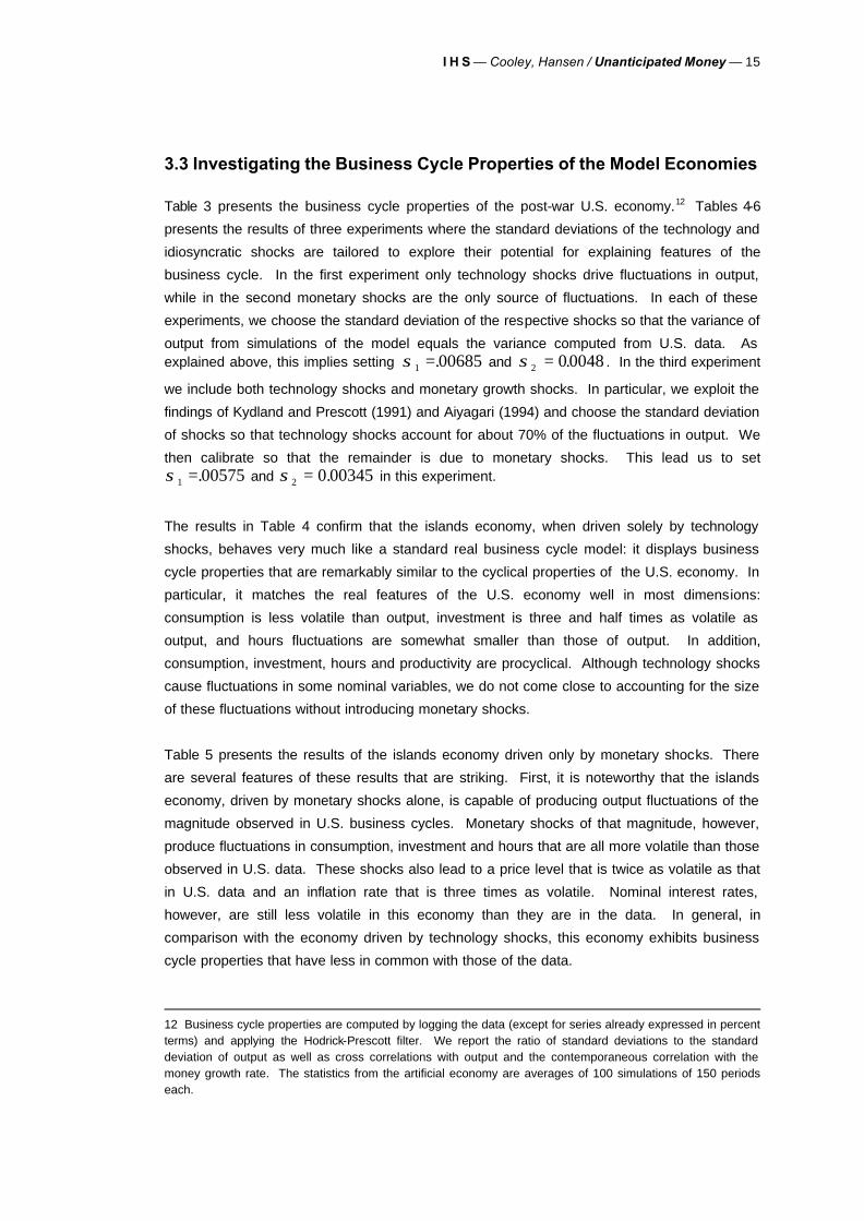
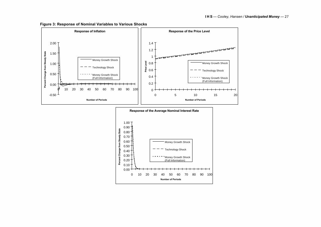
In Figure 3 we show the responses of nominal variables to the same set of shocks. In addition,
we compare the response to a misperceived money growth shock with the response to
perfectly observed money growth shock. The responses look quite similar in both cases. In
particular, the response of the nominal interest rate is exactly the same in both cases. The
inflation responses are somewhat different, however. The initial response of inflation to a
misperceived money growth shock is almost twice as large at the response to perfectly
observed money growth shock.
I H S — Cooley, Hansen / Unanticipated Money — 15
3.3 Investigating the Business Cycle Properties of the Model Economies
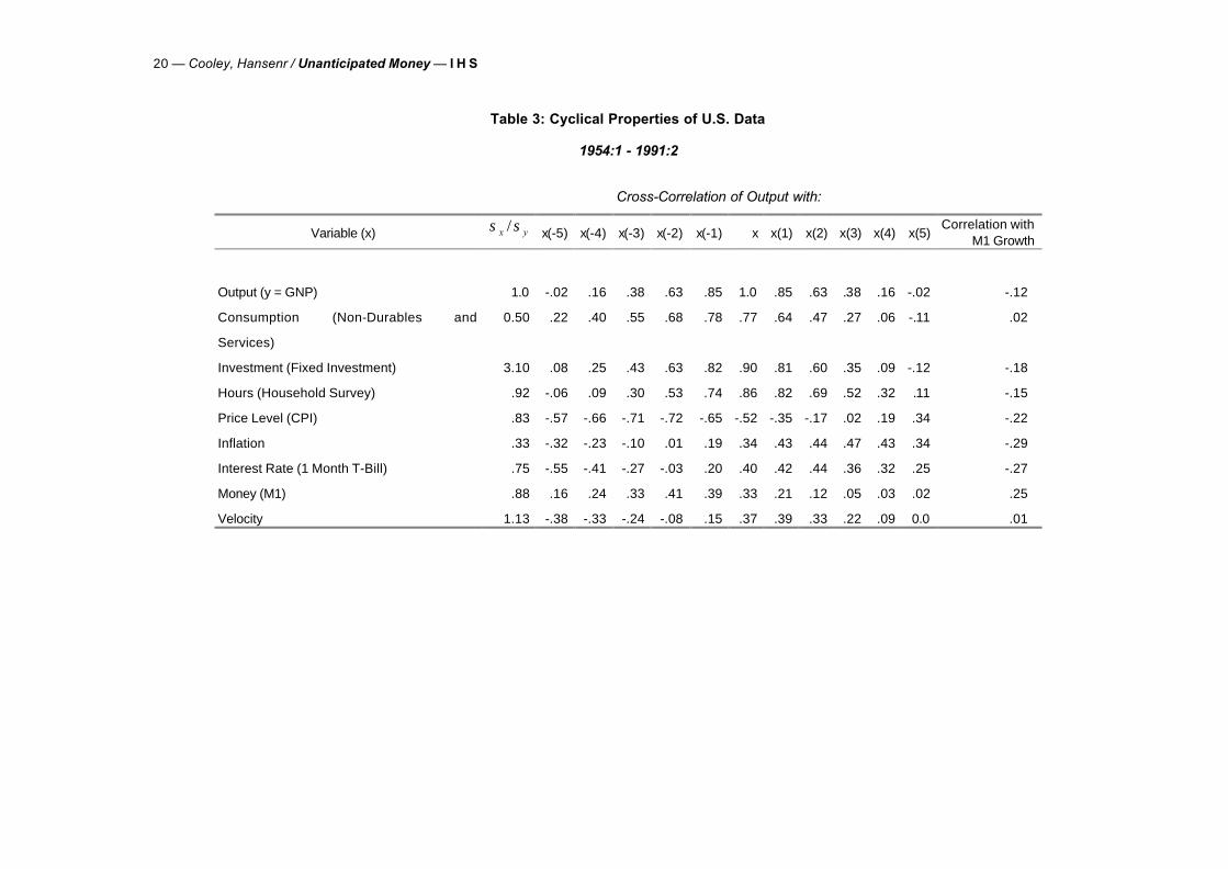
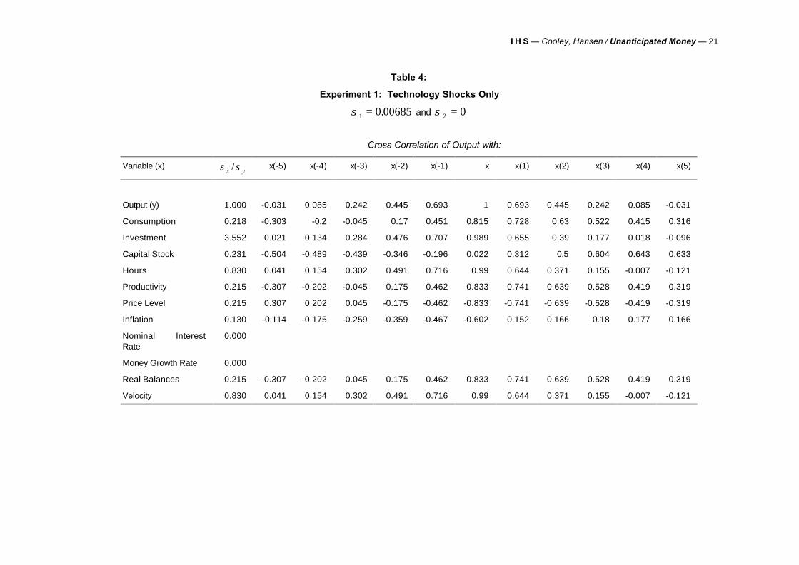
Table 3 presents the business cycle properties of the post-war U.S. economy.12 Tables 4-6
presents the results of three experiments where the standard deviations of the technology and
idiosyncratic shocks are tailored to explore their potential for explaining features of the
business cycle. In the first experiment only technology shocks drive fluctuations in output,
while in the second monetary shocks are the only source of fluctuations. In each of these
experiments, we choose the standard deviation of the respective shocks so that the variance of
output from simulations of the model equals the variance computed from U.S. data. As explained above, this implies setting σ1 00685=. and σ2 00048= . . In the third experiment
we include both technology shocks and monetary growth shocks. In particular, we exploit the
findings of Kydland and Prescott (1991) and Aiyagari (1994) and choose the standard deviation
of shocks so that technology shocks account for about 70% of the fluctuations in output. We
then calibrate so that the remainder is due to monetary shocks. This lead us to set σ1 00575=. and σ2 0 00345= . in this experiment.
The results in Table 4 confirm that the islands economy, when driven solely by technology
shocks, behaves very much like a standard real business cycle model: it displays business
cycle properties that are remarkably similar to the cyclical properties of the U.S. economy. In
particular, it matches the real features of the U.S. economy well in most dimensions:
consumption is less volatile than output, investment is three and half times as volatile as
output, and hours fluctuations are somewhat smaller than those of output. In addition,
consumption, investment, hours and productivity are procyclical. Although technology shocks
cause fluctuations in some nominal variables, we do not come close to accounting for the size
of these fluctuations without introducing monetary shocks.
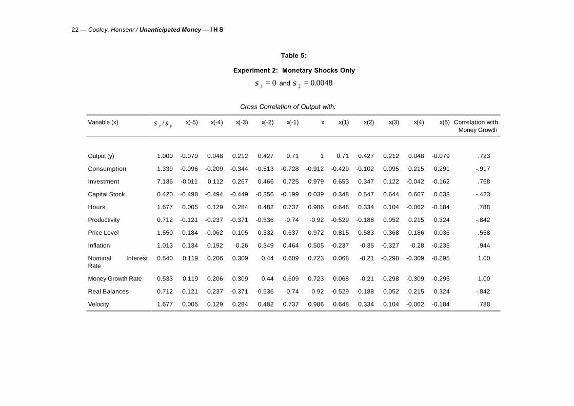
Table 5 presents the results of the islands economy driven only by monetary shocks. There
are several features of these results that are striking. First, it is noteworthy that the islands
economy, driven by monetary shocks alone, is capable of producing output fluctuations of the
magnitude observed in U.S. business cycles. Monetary shocks of that magnitude, however,
produce fluctuations in consumption, investment and hours that are all more volatile than those
observed in U.S. data. These shocks also lead to a price level that is twice as volatile as that
in U.S. data and an inflation rate that is three times as volatile. Nominal interest rates,
however, are still less volatile in this economy than they are in the data. In general, in
comparison with the economy driven by technology shocks, this economy exhibits business
cycle properties that have less in common with those of the data.
12 Business cycle properties are computed by logging the data (except for series already expressed in percent terms) and applying the Hodrick-Prescott filter. We report the ratio of standard deviations to the standard deviation of output as well as cross correlations with output and the contemporaneous correlation with the money growth rate. The statistics from the artificial economy are averages of 100 simulations of 150 periods each.

16 — Cooley, Hansen / Unanticipated Money — I H S
Some of the nominal features of the islands economy mimic features of the U.S. economy
better than the standard cash-in-advance model [see Cooley and Hansen (1995)]. In the
islands economy, inflation, nominal interest rates, and velocity are all procyclical . The price
level, however, is also procyclical in contrast to the data.
The most striking failures of this version of the islands economy is the finding that consumption
and productivity are counter-cyclical. As explained above, the consumption correlation is a
consequence of the way this particular islands economy is structured in that consumption
alone has the role of “shock absorber”. When agents are fooled by a monetary shock they
have to reduce their consumption in order to increase investment.
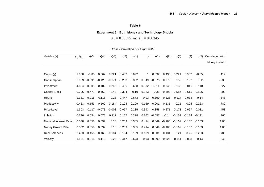
Table 6 presents results for the economy driven by both monetary and technology shocks. As
in the previous experiment, the relative volatility of real variables with respect to output are too
large. The real business cycle properties are, however, closer to those observed in the data
than are the results in Table 5. In addition, as in Table 5, there is a positive contemporaneous
correlation between output and inflation, interests rates, and velocity. However, the major
failings of this as a model of the business cycle remain. Consumption and productivity are
counter-cyclical and the price level is procyclical, although not as strongly as in the economy
driven only by monetary shocks.
Concluding Comments
Previous attempts, such as Kydland (1989) and Cooley and Hansen (1995), to study the
quantitative implications of the Lucas (1972) “islands” economy have reached a pessimistic
assessment of the ability of such an economy to produce much in the way of output
fluctuations. Our findings suggest this conclusion was somewhat misleading. When the
important elements of an islands economy are incorporated, monetary shocks can have
powerful real effects and the resulting fluctuations display some (not all) of the real and nominal
features of the business cycle.
Clearly the findings contained in this paper indicate that our version of the islands model does
not account for the business cycle features of U.S. data as well as a standard real business
cycle model. However, we interpret our findings as suggesting that the Lucas model may have
been abandoned prematurely. Further experimentation with modified versions of this model
economy seem warranted.
I H S — Cooley, Hansen / Unanticipated Money — 17
References
Aiyagari, S. Rao (1994), “On The Contribution of Technology Shocks to Business Cycles,”
Federal Reserve Bank of Minneapolis Quarterly Review, 18, 22-34.
Cooley, Thomas F. and Gary D. Hansen (1989), "The Inflation Tax in a Real Business Cycle
Model," American Economic Review, 79, 733-48.
___________________ (1995), “Money and the Business Cycle,” in Thomas F. Cooley, ed.,
Frontiers of Business Cycle Research, Princeton: Princeton University Press, 175-216.
Cooley, Thomas F. and Edward C. Prescott (1995), Economic Growth and Business Cycles,”
in Thomas F. Cooley, ed., Frontiers of Business Cycle Research, Princeton: Princeton
University Press, 1-38.
Hansen, Gary D. (1985), "Indivisible Labor and the Business Cycle," Journal of Monetary
Economics 16: 309-328.
Hansen, Gary D. and Edward C. Prescott (1995), "Recursive Methods for Computing Equilibria
of Business Cycle Models," in Thomas F. Cooley, ed., Frontiers of Business Cycle
Research, Princeton: Princeton University Press, 39-64.
Kydland, Finn E. (1989), “The Role of Money in a Business Cycle Model,” Institute for
Empirical Macroeconomics Discussion Paper 23, Federal Reserve Bank of Minneapolis.
Kydland, Finn E. and Edward C. Prescott (1982), "Time to Build and Aggregate Fluctuations,"
Econometrica 50: 1345-1370.
___________________ (1991), “Hours and Employment Variation in Business Cycle Theory,”
Economic Theory 1, 63-81.
Lucas, Robert E., Jr. (1972), “Expectations and the Neutrality of Money,” Journal of Economic
Theory 4: 103-123.
___________________ (1975), “An Equilibrium Model of the Business Cycle,” Journal of
Political Economy 83: 1113-1144.
___________________ (1977), “Understanding Business Cycles,” in Karl Brunner and Alan
Meltzer, eds., “Stabilization of the Domestic and International Economy, Amsterdam:
North Holland.

18 — Cooley, Hansen / Unanticipated Money — I H S
Lucas, Robert E., Jr. and Nancy L. Stokey (1987), “Money and Interest in a Cash-in-Advance
Economy,” Econometrica 55: 491-514.
Mood, A.M., F.A. Graybill and D.C. Boes (1974), Introduction to the Theory of Statistics, New
York: McGraw-Hill.
Rogerson, Richard (1988), "Indivisible Labor, Lotteries and Equilibrium," Journal of Monetary
Economics 21: 3-16.
I H S — Cooley, Hansen / Unanticipated Money — 19
Table 1: Parameter Values
β α γ θ δ ρ1 ρ2 σ2 ρ3 µ
0.989 0.84 2.556 0.4 0.019 0.95 0.49 0.0089 0.99 0.015
Table 2: Decision Rules for Full Information Version of Model:
log $P = 1.62570 - 0.34704 z + 6.35763 s + 0 g - 0.54626 log K
log K'= 0.11324 + 0.12945 z + 1.21562 s + 0 g + 0.96393 log K
log H = -0.02343 + 1.63229 z + 15.89330 s + 0 g - 0.36561 log K
20 — Cooley, Hansenr / Unanticipated Money — I H S
Table 3: Cyclical Properties of U.S. Data
1954:1 - 1991:2
Cross-Correlation of Output with:
Variable (x) σ σx y/ x(-5) x(-4) x(-3) x(-2) x(-1) x x(1) x(2) x(3) x(4) x(5) Correlation with
M1 Growth
Output (y = GNP) 1.0 -.02 .16 .38 .63 .85 1.0 .85 .63 .38 .16 -.02 -.12
Consumption (Non-Durables and
Services)
0.50 .22 .40 .55 .68 .78 .77 .64 .47 .27 .06 -.11 .02
Investment (Fixed Investment) 3.10 .08 .25 .43 .63 .82 .90 .81 .60 .35 .09 -.12 -.18
Hours (Household Survey) .92 -.06 .09 .30 .53 .74 .86 .82 .69 .52 .32 .11 -.15
Price Level (CPI) .83 -.57 -.66 -.71 -.72 -.65 -.52 -.35 -.17 .02 .19 .34 -.22
Inflation .33 -.32 -.23 -.10 .01 .19 .34 .43 .44 .47 .43 .34 -.29
Interest Rate (1 Month T-Bill) .75 -.55 -.41 -.27 -.03 .20 .40 .42 .44 .36 .32 .25 -.27
Money (M1) .88 .16 .24 .33 .41 .39 .33 .21 .12 .05 .03 .02 .25
Velocity 1.13 -.38 -.33 -.24 -.08 .15 .37 .39 .33 .22 .09 0.0 .01
I H S — Cooley, Hansen / Unanticipated Money — 21
Table 4:
Experiment 1: Technology Shocks Only
σ1 0 00685= . and σ2 0=
Cross Correlation of Output with:
Variable (x) σ σx y/ x(-5) x(-4) x(-3) x(-2) x(-1) x x(1) x(2) x(3) x(4) x(5)
Output (y) 1.000 -0.031 0.085 0.242 0.445 0.693 1 0.693 0.445 0.242 0.085 -0.031
Consumption 0.218 -0.303 -0.2 -0.045 0.17 0.451 0.815 0.728 0.63 0.522 0.415 0.316
Investment 3.552 0.021 0.134 0.284 0.476 0.707 0.989 0.655 0.39 0.177 0.018 -0.096
Capital Stock 0.231 -0.504 -0.489 -0.439 -0.346 -0.196 0.022 0.312 0.5 0.604 0.643 0.633
Hours 0.830 0.041 0.154 0.302 0.491 0.716 0.99 0.644 0.371 0.155 -0.007 -0.121
Productivity 0.215 -0.307 -0.202 -0.045 0.175 0.462 0.833 0.741 0.639 0.528 0.419 0.319
Price Level 0.215 0.307 0.202 0.045 -0.175 -0.462 -0.833 -0.741 -0.639 -0.528 -0.419 -0.319
Inflation 0.130 -0.114 -0.175 -0.259 -0.359 -0.467 -0.602 0.152 0.166 0.18 0.177 0.166
Nominal Interest Rate
0.000
Money Growth Rate 0.000
Real Balances 0.215 -0.307 -0.202 -0.045 0.175 0.462 0.833 0.741 0.639 0.528 0.419 0.319
Velocity 0.830 0.041 0.154 0.302 0.491 0.716 0.99 0.644 0.371 0.155 -0.007 -0.121
22 — Cooley, Hansenr / Unanticipated Money — I H S
Table 5:
Experiment 2: Monetary Shocks Only
σ1 0= and σ2 0 0048= .
Cross Correlation of Output with:
Variable (x) σ σx y/ x(-5) x(-4) x(-3) x(-2) x(-1) x x(1) x(2) x(3) x(4) x(5) Correlation with Money Growth
Output (y) 1.000 -0.079 0.048 0.212 0.427 0.71 1 0.71 0.427 0.212 0.048 -0.079 .723
Consumption 1.339 -0.096 -0.209 -0.344 -0.513 -0.728 -0.912 -0.429 -0.102 0.095 0.215 0.291 -.917
Investment 7.136 -0.011 0.112 0.267 0.466 0.725 0.979 0.653 0.347 0.122 -0.042 -0.162 .768
Capital Stock 0.420 -0.498 -0.494 -0.449 -0.356 -0.199 0.039 0.348 0.547 0.644 0.667 0.638 -.423
Hours 1.677 0.005 0.129 0.284 0.482 0.737 0.986 0.648 0.334 0.104 -0.062 -0.184 .788
Productivity 0.712 -0.121 -0.237 -0.371 -0.536 -0.74 -0.92 -0.529 -0.188 0.052 0.215 0.324 -.842
Price Level 1.550 -0.184 -0.062 0.105 0.332 0.637 0.972 0.815 0.583 0.368 0.186 0.036 .558
Inflation 1.013 0.134 0.192 0.26 0.349 0.464 0.505 -0.237 -0.35 -0.327 -0.28 -0.235 .944
Nominal Interest Rate
0.540 0.119 0.206 0.309 0.44 0.609 0.723 0.068 -0.21 -0.298 -0.309 -0.295 1.00
Money Growth Rate 0.533 0.119 0.206 0.309 0.44 0.609 0.723 0.068 -0.21 -0.298 -0.309 -0.295 1.00
Real Balances 0.712 -0.121 -0.237 -0.371 -0.536 -0.74 -0.92 -0.529 -0.188 0.052 0.215 0.324 -.842
Velocity 1.677 0.005 0.129 0.284 0.482 0.737 0.986 0.648 0.334 0.104 -0.062 -0.184 .788
I H S — Cooley, Hansen / Unanticipated Money — 23
Table 6
Experiment 3: Both Money and Technology Shocks
σ1 0 00575= . and σ2 0 00345= .
Cross Correlation of Output with:
Variable (x) σ σx y/ x(-5) x(-4) x(-3) x(-2) x(-1) x x(1) x(2) x(3) x(4) x(5) Correlation with
Money Growth
Output (y) 1.000 -0.05 0.062 0.221 0.433 0.692 1 0.692 0.433 0.221 0.062 -0.05 .414
Consumption 0.939 -0.091 -0.125 -0.174 -0.233 -0.302 -0.349 -0.075 0.079 0.159 0.192 0.2 -.935
Investment 4.884 -0.001 0.102 0.246 0.436 0.668 0.932 0.611 0.345 0.136 -0.016 -0.118 .627
Capital Stock 0.296 -0.471 -0.463 -0.42 -0.334 -0.19 0.023 0.31 0.492 0.587 0.615 0.596 -.309
Hours 1.151 0.015 0.118 0.26 0.447 0.673 0.93 0.599 0.326 0.114 -0.038 -0.14 .648
Productivity 0.423 -0.153 -0.169 -0.184 -0.194 -0.199 -0.169 0.001 0.131 0.21 0.25 0.263 -.780
Price Level 1.303 -0.117 -0.073 -0.003 0.097 0.235 0.393 0.358 0.271 0.178 0.097 0.031 .458
Inflation 0.796 0.054 0.075 0.117 0.167 0.228 0.262 -0.057 -0.14 -0.152 -0.134 -0.111 .960
Nominal Interest Rate 0.538 0.058 0.097 0.16 0.239 0.335 0.414 0.049 -0.106 -0.162 -0.167 -0.153 1.00
Money Growth Rate 0.532 0.058 0.097 0.16 0.239 0.335 0.414 0.049 -0.106 -0.162 -0.167 -0.153 1.00
Real Balances 0.423 -0.153 -0.169 -0.184 -0.194 -0.199 -0.169 0.001 0.131 0.21 0.25 0.263 -.780
Velocity 1.151 0.015 0.118 0.26 0.447 0.673 0.93 0.599 0.326 0.114 -0.038 -0.14 .648
24 — Cooley, Hansenr / Unanticipated Money — I H S
Figure 1: Perceived Island Specific Shock in Response to a Money Growth Shock
Perceived Value of s
0.0000
0.0002
0.0004
0.0006
0.0008
0.0010
0.0012
0 10 20 30 40 50 60 70 80 90 100N u m b e r o f P e r i o d s
I H S — Cooley, Hansen / Unanticipated Money — 25
Figure 2: Response of Real Variables to Various Shocks
Response of Consumption
-2.50
-2.00
-1.50
-1.00
-0.50
0.00
0.50
1.00
0 10 20 30 40 50 60 70 80 90 100
Number of Periods
Per
cent
Cha
nge
from
Ste
ady
Sta
te
Money Growth Shock
Technology Shock
Response of Investment
-1.00
0.001.00
2.003.00
4.005.00
6.007.00
8.009.00
0 10 20 30 40 50 60 70 80 90 100Number of Periods
Per
cent
Cha
nge
from
Ste
ady
Sta
te
Money Growth Shock
Technology Shock
Response of Hours Worked
-0.50
0.00
0.50
1.00
1.50
2.00
2.50
0 10 20 30 40 50 60 70 80 90 100
Number of Periods
Per
cent
Cha
nge
from
Ste
ady
Sta
te
Money Growth Shock
Technology Shock
Response of Capital
0.000.100.20
0.300.40
0.500.600.70
0.800.901.00
0 10 20 30 40 50 60 70 80 90 100Number of Periods
Per
cent
Cha
nge
from
Ste
ady
Sta
te
Money Growth Shock
Technology Shock
26 — Cooley, Hansenr / Unanticipated Money — I H S
Figure 2 - Continued
Response of Output
0.00
0.20
0.40
0.60
0.80
1.00
1.20
1.40
1.60
0 10 20 30 40 50 60 70 80 90 100N u m b e r o f P e r i o d s
M o n e y G r o w t h S h o c k
T e c h n o l o g y S h o c k
I H S — Cooley, Hansen / Unanticipated Money — 27
Figure 3: Response of Nominal Variables to Various Shocks
Response of Inflation
-0.50
0.00
0.50
1.00
1.50
2.00
0 10 20 30 40 50 60 70 80 90 100
Number of Periods
Per
cent
Cha
nge
from
Ste
ady
Sta
te
Money Growth Shock
Technology Shock
Money Growth Shock(Full Information)
Response of the Price Level
0
0.2
0.4
0.6
0.8
1
1.2
1.4
0 5 10 15 20Number of Periods
Pric
e Le
vel
Money Growth Shock
Technology Shock
Money Growth Shock(Full Information)
Response of the Average Nominal Interest Rate
0.000.10
0.200.300.40
0.500.60
0.700.80
0.901.00
0 10 20 30 40 50 60 70 80 90 100Number of Periods
Per
cent
Cha
nge
from
Ste
ady
Sta
te
Money Growth Shock
Technology Shock
Money Growth Shock(Full Information)

Institut für Höhere Studien
Institute for Advanced Studies
Stumpergasse 56
A-1060 Vienna
Austria
Phone: +43-1-599 91-145
Fax: +43-1-599 91-163
Related Documents