INFRARED SPECTROSCOPY OF METHANE DIMERkodu.ut.ee/~jaakk/oppetoo/FKMF_01_054/Supersonic_jet.pdf · gases like diffusion, viscosity and heat capacity, in molecular solids the structure

INFRARED SPECTROSCOPY OF METHANE

DIMER

By

Abdullah Hamdan

A thesis submitted to the

Faculty of the Graduate School of

Ruhr-Universität Bochum in fulfillment of the

requirements for the doctor rer. nat

Department of Chemistry

December 2005

Abstract:

Rotationally resolved infrared spectra of methane dimer complex have been detected for

the first time in the R (0) spectral region of the triply degenerate bending mode of

methane monomer using tunable diode laser spectrometer along with supersonic jet

system. Methane dimer lines were confirmed by scanning the desired wavelength regions

with a mixture of 40% methane in Ar and He-Ne separately and then exclude the CH4-Ar

and CH4-Ne spectral lines. Many dimer lines are observed between 1290 and 1320 cm-1

,

but the lines are found to be more concentrated after the band center of the bending mode

of CH4 monomer. The spectra exhibit well resolved R branch, while the P and Q branches

have been predicted. A Hamiltonian model based on Coriolis coupling model was used to

assign and fit the recorded spectrum to within 20-30 MHz accuracy. The calculated value

of the effective rotational quantum number (j*) conclude that methane molecule is close

to free rotor limit in the complex.

Dedication

To My Wife

Acknowledgements

Praise be to God (Allah), who gave me the strength and the patience and who bestowed

his boundless mercy on me to accomplish this work.

I would like first to express my profound gratitude and appreciation to Prof. Martina

Havenith Newen for giving me the opportunity to join her very well established research

group and a well equipped laboratory to work for my PhD. It is really fortunate to work

with such group like that. Thank you so much Frau Havenith for the continual

enthusiasm, guidance, encouragement, and all kinds of support that I received over the

years of my study in the RUB-Germany.

I am also extremely grateful to Dr. Gerhard Schwaab who has always been of great and

remarkable assist in all stages of completing my PhD project. My words cannot really

thank him enough for his endless help and his welling always to work out and discuss all

the related issues in the experiment as well as in the writing up this thesis. Thanks a lot

for everything Gerhard.

I would like also to record my thankful to Dr. Erik Bruendermann for the fruitful

discussions on some of the primary results using the previous version of the fitting

program, helping in the lab from time to time and his great computer support.

A lot of thanks to Dr. Guido Gimmler who put a great efforts in training me and

explaining many details about the diode laser spectrometer and the supersonic jet

technique which helped me to be in control of the system.

I want also to thank my friend Rachael for translating some scientific materials which

were of good help for me in this project.

My thanks extend to the secretaries of the department specially Frau Ulla Knieper who

has been welling always to help and advise me in managing all kind of related issues

regarding my legal stay and legal rights during my studying period in Germany.

Thanks to Mr. Christian Fester and Mr. Reinhard Renzewitze for their prompt positive

reaction for seeking their help in the lab.

Finally, I would like to thank all my colleagues who helped me in one way or another to

finish this work.

List of Contents.

1. Introduction. 1 1.1 Molecular Forces

1.2 Origin of Van der Waals Forces

1.3 Importance of Van der Waals Forces

2. The Theory of Intermolecular Interactions. 6

2.1 The Electrostatic energy.

2.2 Dipole-Induced-Dipole Interactions.

2.3 Dispersion Interactions.

2.4 Repulsive Interactions.

3. Methane hydrates-A potential Energy Source of the 21st Century. 11

3.1 Methane Definition

3.2 Methane Production

3.3 Methane Hydrates

3.3.1 Definition

3.3.2 Historical Perspective

3.3.3 Crystal Structure

3.4 Phase Equilibrium

3.5 Occurrence and Locations (Global Distribution)

3.6 Estimated Amounts

3.7 Energy Prospects

4. Experimental Apparatus. 25 4.1 The Tunable Diode Laser Spectrometer.

4.1.1 Laser Source

4.1.2 Cryostat

4.2 Supersonic Molecule Jet Apparatus.

4.2.1 Types of Expansions

4.2.2 Pulsed Slit Nozzles

4.3 Possible Detection Methodes

4.3.1 The Rapid-Scan Method

4.3.2 The Step-Scan Method

4.4 Set-Up and Operation of Pulsed Slit Nozzle

5. The Infrared Spectroscopy of Methane Complexes. 51

6 The Theory of Symmetric Top Rotors. 62 6.1 Symmetric Top Molecules

6.2 Asymmetric Top Molecules

6.3 Selection Rules

6.4 Perturbations

6.5 Degeneracy

7 Coriolis Force

7. Measurements and Discussion. 81 7.1 Symmetry of Tetrahedral Molecules

7.2 Data Analysis

8. References 103

1

___________________________________________________________________________

CHAPTER 1

Introduction

___________________________________________________________________________

Forces between atoms and molecules have attracted research interest for more than a

century especially in the field of spectroscopy. The development of both high

resolution experimental and theoretical techniques in this field particularly in the last

few decades made a big jump in the knowledge and understanding of these forces

possible. Infrared spectroscopy is the most common and versatile spectroscopic

technique used mainly by chemists to study the physical and chemical properties of

different types of all possible materials in the three states of matter. The main

objective is to determine the chemical and dynamical structure of the investigated

samples by targeting the molecular forces present in the molecular sample. Therefore,

this introductory chapter aims to give a brief description in rather simple way on the

different types of molecular forces acting between atoms and molecules, the origin

and the importance of these forces in life.

1.1 Molecular forces

Intramolecular and intermolecular forces are the two types of molecular forces that

are responsible for keeping and holding the atoms and molecules united to form the

different fascinating and splendid shapes of the three states of matter. Intramolecular

refers to the covalent, ionic and metallic bond forces that are acting between the atoms

within the molecule and from which the chemical properties of the matter can be

extracted (1, 2)

. On the other hand, ´intermolecular` refers to the dispersion, induction

and electrostatic bond forces that are acting between molecules. These forces are also

known as Van der Waals forces and can be used to characterize the dynamical

structure of the molecular complexes. These are also the forces that will be considered

and discussed more here and in the following chapter. The Van der Waals complexes

are characterized by extremely weak binding energies which lie in the range of 10-

100cm-1

and hence lead to very long bond lengths in the complex. Hydrogen bonding

2

is also another form of the intermolecular forces but does not belong to the same

category of Van der Waals interactions. They are the strongest intermolecular forces

with bond energies of 100-1000 cm-1

; this range is still at least 1 to 2 orders of

magnitude weaker than the energy of normal chemical bonds which exhibit bond

energies between 104 and 10

5 cm

-1. This is the reason why Van der Waals complexes

are only stable at very low temperatures, when their average thermal energies lie

below their bond energies which leads to long intermolecular bond lengths in the

aggregates of about 3-4 Ao.

1.2 Origin of Van der Waals forces

By the mid of 19th

century, the kinetic theory of gases confirmed the fact that atoms

and molecules are the basic blocks of matter. At the same time it also neglected the

volume and the intermolecular forces of molecules which led to the break down of the

ideal gas law when gases are put under conditions of high pressure and low

temperature. In 1873 the Dutch physicist Johannes van der Waals was the first to

incorporate these ideas along with the results of his experiments on pure gases to

develop an equation that was known later as van der Waals equation which describes

the behavior of real gases compared to ideal gases.

(P + a n2/V

2)(V – n b) = n R T

where P, V, n, R, T are pressure, volume, number of molecules, Boltzmann constant

and temperature respectively. The constant "a" is a correction term for intermolecular

force while "b" is the correction term for the real volume of the gas molecules.

The equation indicates that the actual free volume of the container is reduced by the

molecules occupied volume of the molecules which implies that strong repulsive

forces are effective at short distances. The equation also suggests that the gas pressure

is actually slightly less than it would be without attractive forces which lead to the

conclusion that long range intermolecular forces are effective. These forces were

believed to be of classical electrostatic origins, but the development of the quantum

mechanical methods led to conclude that these forces have also quantum mechanical

character (3)

.

3

Intermolecular interactions originate from the fact that atoms and molecules are

composed of charged particles which interact by the means of Coulomb forces. The

quantum mechanical treatment of these forces can lead to the following

intermolecular interactions; electrostatic, induction, dispersion, and exchange

repulsion. The first order perturbation theory describes the electrostatic and the

exchange repulsion contributions, while the induction and dispersion components

occur in second order perturbation theory. The electrostatic components originate

from classical interaction between static charge distributions of two polar molecules

leading to the dipole-dipole interactions. The induction contributions arise from the

distortion of a particular unpolar molecule by the electric field of all other

neighbouring molecules. The dispersion energy is a result of quantum fluctuation of

the electron distributions on atoms or molecules leading to the induced dipole-induced

dipole interaction even for the most symmetrical systems. The exchange-repulsion

forces are the short-range forces which occur as consequence of strong repulsion

between strongly overlapped and occupied orbitals of neighboring atoms or

molecules. The theory of these forces (interactions) will be discussed in the following

chapter (3)

.

There has been a lot of scientific interest on investigating small weakly bound van der

Waals complexes for the last few decades in order to understand the mechanism of

intermolecular interactions. But in spite of its long history, it was possible to examine

these complexes with high resolution spectroscopic techniques only 20-30 years ago.

The experimental and theoretical advances in this field have been documented in 3

complete editions of “Chemical Reviews” (4, 5, 6)

.

1.3 Importance of Van der Waals forces

Intermolecular forces are feeble; but without them all matter would exist in a gaseous

state, and life as we know it would be impossible. They form the basis of a wide range

of fundamental scientific phenomena in different branches of physics, chemistry and

biology. Many physical and chemical properties (e.g. melting points, boiling points,

heats of fusion and vaporization, surface tension, densities …etc) of molecular

compounds, including crystal structures, depend mainly on intermolecular forces. For

instance, in the gaseous phase they are responsible for the transport properties of

4

gases like diffusion, viscosity and heat capacity, in molecular solids the structure of

molecular crystals depends very much on the anisotropy of the intermolecular

potentials between the individual molecules, and the solvation processes in liquids are

determined only by intermolecular interactions.

They also play a central role in biology and life sciences, being responsible for

holding gigantic molecules like enzymes, proteins, and DNA into their original and

required shapes. The biological relevance of hydrogen bonds is due to their lack of

strength; they are stable at room temperature but can be easily broken by a small

amount of energy input, which allows changes in the stable configuration. This is how

the genetic code on DNA is replicated. It was also reported that intermolecular forces

can act as the mediator of some protein receptor-drug reactions (7, 8, 9)

. Investigation of

Van der Waals complexes started first with the closed-shell molecular species. The

open-shell molecular species started recently to attract more research interest,

especially the ones that form in the atmosphere and the interstellar clouds as many of

their properties are poorly understood. It is well known that these complexes are

expected to have a profound effect on the chemistry of the atmosphere as a result of

relatively low temperature, production of many free radicals and the effects of

radiation (10)

. These examples are just some of many other phenomena that depend on

intermolecular interactions.

From the above examples, one can realize how essential these weak forces are in our

life, and how crucial it is to have an accurate theoretical description of these forces

especially for large systems like DNA molecules. Therefore, it is highly desirable to

obtain a simple and reliable model that can be tested first on relatively small prototype

Van der Waals complexes to help understand the existing interactions. The results can

then be expanded to more complex systems and thus used to develop an exact model

of the Van der Waals forces between the molecules.

Infrared spectroscopic techniques are, in principle, the techniques that are used to

serve in achieving the above goal experimentally. These techniques are used to

measure inter- intermolecular vibrational modes of the weakly bound complexes and

thus determine the positions of their energy levels. Experimental results are then used

to help determine accurate intermolecular potential surfaces. Modeling the potentials

5

from many of these small prototype systems can give a general understanding of the

interactions in larger systems. Moreover, high resolution infrared spectra can also

provide detailed information about the dynamics and structure of molecular

complexes in both ground and electronically excited states. The molecular constants

extracted from the infrared spectra are directly related to the geometrical structures in

both states, giving access to information about intermolecular bond lengths and their

changes upon excitation. For example, if there is tunneling present within the

complex, it becomes apparent in the splitting of the rotation lines in the spectrum.

6

___________________________________________________________________________

CHAPTER 2

Theory of intermolecular forces

___________________________________________________________________________

Investigation of intermolecular forces started practically with the developments of

both high resolution experimental and computational techniques about thirty years

ago. These studies led to numerous advances in the knowledge and understanding of

these forces especially in the last decade where a lot of progress has been achieved in

the construction of reliable intermolecular potential energy surfaces from which

various chemical and physical properties of the molecular system can be extracted.

Intermolecular potentials are also important and necessary for the determination of the

structure, stability, and dynamics of weakly bound clusters and condensed phases.

The molecular interactions described by these potentials depend mainly on the

distance between the involved molecules and their relative orientation to each other.

Intermolecular potentials can not be measured directly from experiments. Different

theoretical computational approaches are used to derive intermolecular potentials.

According to their point of origin, these approaches are grouped into two classes: the

semi-empirical and quantum mechanical potentials. In the first approach the

intermolecular potentials (PES) can be inferred from experimental data from different

experimental sources such as spectroscopic measurements, second virial coefficients

and molecular-beam scattering data, but in this case it is important here to assume

some functional form of the interaction and attempt to vary the parameters of the fit to

reproduce the experimental results. Another approach to the PES is via ab initio

quantum mechanical calculations, where the molecular potentials are calculated

theoretically using the electronic molecular orbital theory. This method has been

lately improved by the growth of the computing power.

The theory of intermolecular interactions and its contributions is described in different

articles and books (3, 11, 12)

. It has four main energy contributions which are classified

as long-range forces; electrostatic, induction, and dispersion and short-range forces

7

like the exchange-repulsion force. These forces will be briefly discussed in this

section

2.1 Electrostatic Energy

Electrostatic forces are the energy contributions that occur between the charged

particles of molecules with permanent dipole moment which can be classically

represented by the Coulomb interaction law between the individual complex-building

molecules. In general, all electrostatic charges in the molecule have to be taken into

account to calculate the Coulomb potential of the system, i.e. all electrons and nuclei

in the molecular system are contributing to the overall potential. The Coulomb

potential energy is given as:

∑=ij ij

ji

electR

qqV

π4 (2.1)

where qi is the charge on the i-th particle and Rij is the distance between the i-th and

the j-th particle.

As a result of their long range behavior, these interactions will have substantial

contribution to the intermolecular potential energy. The consequence of 1/R

dependency leads to conclude that the electrostatic potential will contribute to the

total energy much more than from dispersion energy at larger distances. The

electrostatic components of the intermolecular potential are strictly pair wise additive

and it can be attractive or repulsive depending on the orientation of the two monomers

(3, 13, 14).

The interaction energy of two permanent dipoles depends on the relative orientation

of both dipoles which could be zero if all the orientations are possible. This can be

true if the molecules are completely free to rotate, but in practice molecules are not

totally free to rotate and some orientations are preferred over others. Therefore, the

interaction energy varies as 1/ R6, while the force between the dipoles varies as 1/R

7.

In a solid sample the interaction energy varies as 1/ R3 (3)

.

8

2.2 Induction Energy (Dipole – Induced – Dipole Interaction)

The energy contributions here emerge when a molecule with a permanent dipole

moment induces a dipole moment in a neighboring polarizable molecule. This

interaction creates an attractive atmosphere between the two dipoles. Therefore, the

induction forces are always attractive. The strength of this interaction is a function of

the electric field E of the permanent dipole and the polarizability α of the neighboring

molecule. The induction energy is given by:

2

2

1EV ind α= (2.2)

Induction energy is severely non-additive depending on the direction of the multipole

moment, i.e. when a molecule is surrounded by other neighbor molecules, the electric

fields of the surrounding molecules may reinforce or cancel each other.

The second-order perturbation theory indicates that if one monomer possesses electric

dipole moment, the magnitude of induction energy varies as R-6

, where R is the

distance between the molecules. The induction energy delivers a non-zero

contribution also if only one bond partner has a multipole moment (3)

.

2.3 Dispersion Energy (Induced Dipole – Induced Dipole Interaction)

It is also known as London dispersion forces or Van der Waal force. This contribution

is of a purely quantum mechanical nature and cannot be explained classically. In

principle, all molecules have the possibility to form London forces. But they mainly

occur between nonpolar atoms or molecules such as (noble gases, N2, H2, O2…CH4,

CCl4, BF3…etc). These are the weakest intermolecular forces which arise from the

fluctuations of the charge density distribution in atoms or molecules as a result of

constant motion of electrons leading to a temporary dipole. These transient dipole

moments cancel out each other to zero over a certain period of time, but the molecule

can still interact with neighboring molecules at any time. This in turn can induce an

instantaneous dipole moment in a second molecule and hence result in building up a

net attractive force between the two molecules. The electrons in both molecules then

become correlated which leads to the favored lower energy configuration of the

9

complex. These dipoles depend on the polarizability of the molecule, and vary as

1/R6. Dispersion forces increases with mass, number of atoms or electrons which

reflect on certain properties of materials.

An exact theory of the dispersion interaction naturally includes the higher order

multipole moments. The dispersion energy is obtained from the second order

correction of the perturbation theory and is given as:

Vdis = C6 R-6

+ C8 R-8

+ C10 R-10

+ …. (2.3)

The dispersion energy has much more isotropic properties than the electrostatic or the

induction energy, because the instantaneous multipole moments can orientate

themselves in any direction relative to the static molecular coordination system (3)

.

2.4 Exchange-Repulsion Energy

The Exchange-Repulsion means that the electron motions can extend over either both

atoms or molecules for the exchange part, whereas the repulsion means that in term of

atomic and molecular orbitals an antibonding orbital can be populated. These are

repulsive forces which exist or operate at very short distances where the wave

functions of atoms or molecules are significantly overlapped, i.e. the charge

distributions/densities of neighboring atoms or molecules are strongly overlapped.

This result in a strong repulsion between the tightly bound electrons which in turn

leads to a reduction in the electron density between the nuclei due to the Pauli

principle and the nuclei then repel each other. The simplest representation of the

repulsive force is a single exponential function:

Vrep = A e-βR

(2.4)

with A and b are two adjustable parameters which depend on the angular orientation

of the two monomers (15)

. This functional relationship is included in several semi-

empirical potentials (16-21)

The individual contribution of the above mentioned intermolecular forces to the

intermolecular potential depends mainly on the symmetry of the charge distribution,

10

the spatial distance between the individual interacting partners and their orientation to

one another. It shows whether a potential minimum is formed between the interacting

molecules and if the formation of a complex is at all possible or not.

The construction of a theoretical model for each of these contributions to the

intermolecular interaction -especially the repulsive and dispersive forces- still remains

a challenge for quantum chemistry up to date.

11

_____________________________________________________________________

CHAPTER 3

Methane Hydrates-a potential energy source of the 21st Century

_____________________________________________________________________

The awareness of methane as a possible energy source began after the discovery of

the natural methane hydrates back in the 1960’s. This discovery triggered many

research groups at the global scale to put more efforts on studying these hydrates

especially in the last two decades. This chapter will briefly discuss the basic concept

as well as the most important and relevant aspects of hydrates concentrating mainly

on methane hydrates.

3.1 Definition

Methane is a colorless, odorless, nontoxic and highly flammable gas with a wide

distribution in nature. At room temperature, methane is lighter than air, melts at –

183°C and boils at –164°C. It belongs to the alkane group of hydrocarbons which are

basically organic compounds that consist only of carbon and hydrogen atoms. These

atoms can combine together in virtually countless ways to make a diversity of

products composing the different groups of hydrocarbons. Methane is the simplest

molecular structure of hydrocarbons with a chemical formula of CH4. It has the

typical tetrahedral shape where the carbon atom is attached or connected to four

hydrogen atoms by single bonds making an angle of 109.5 degrees at room

temperature. Methane constitutes the primary or principal component of natural gas; it

normally makes up 50-90 % of the mixture depending on the source. The balance is a

varying amount of ethane, propane, butane, and other hydrocarbon compounds.

12

3.2 Methane production

Two models are proposed for methane production: thermogenic and biogenic models.

In the thermogenic model, methane is produced by the combined action of heat,

pressure and time on buried organic materials which is mainly the common

mechanism for the production of hydrocarbon gases. In the biogenic model, methane

is formed by anaerobic digestion of certain organic matters (plants, animals,

waste...etc) in areas that are almost oxygen free. The digestion is a two step process

which is mainly done by a special kind of anaerobic bacteria that are usually found in

oxygen poor or oxygen free environments like livestock, landfills and dumps,

wetlands, along side with oil fields inside the earth and shallow sea floor sediments.

The first step is the breakdown of the complex organic waste into simple organic

acidic compounds by a particular group of bacteria, called acid formers. In the second

step, a highly specialized group of bacteria, called methane formers, converts the

acids to methane gas and carbon dioxide. In a properly functioning digester, the two

groups of bacteria must balance so that the methane-formers use just the acids

produced by the acid-formers.

The detailed stages of methane formation have been described by Hesse (22)

, while the

overall of methane production is summarized by Sloan (23)

in the following equation:

(CH2O)106(NH3)16(H2PO4) 53CO2+53CH4+16NH3+H2PO4

The equation summarizes successive stages of oxidation by oxygen and reduction by

nitrates, sulfates, and carbonates.

Methane can also be produced industrially by the destructive distillation of coal or

wood, or by heating certain mixtures like sodium acetate and sodium hydroxide or

carbon and hydrogen, and by the reaction of certain complexes like aluminum carbide

and water.

In addition to the above mentioned different sources of methane production on earth,

methane is also found as a major constituent of the atmospheres of most of the

gaseous planets in our solar system including the earth (24)

.

Since methane is a highly flammable gas and being continuously produced by supply

from biogenic/bacterial emission, methane is used as an alternative source of energy

13

on many different industrial, social, environmental and economical fields of life

worldwide, therefore it is considered to be the most important, versatile, viable,

sustainable and economic molecular gas of hydrocarbons.

On the other hand, methane is an important greenhouse gas with global warming of

25, (i.e, it has 25-30 times the warming ability of carbon dioxide.)

3.3 Methane Hydrates (clathrates)

3.3.1 Definition

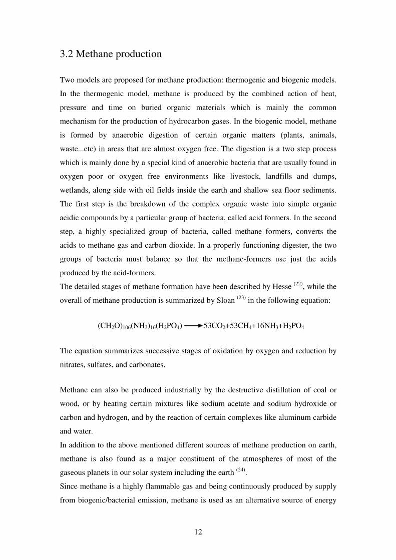
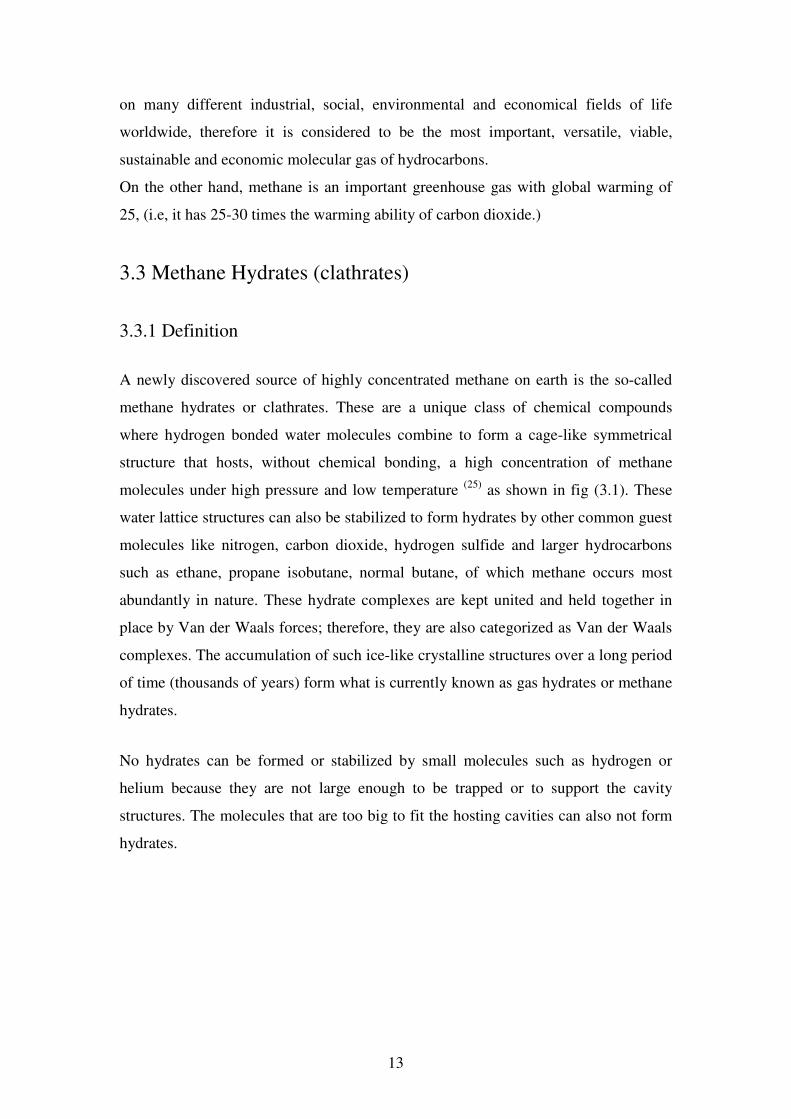
A newly discovered source of highly concentrated methane on earth is the so-called

methane hydrates or clathrates. These are a unique class of chemical compounds

where hydrogen bonded water molecules combine to form a cage-like symmetrical

structure that hosts, without chemical bonding, a high concentration of methane

molecules under high pressure and low temperature (25)

as shown in fig (3.1). These

water lattice structures can also be stabilized to form hydrates by other common guest

molecules like nitrogen, carbon dioxide, hydrogen sulfide and larger hydrocarbons

such as ethane, propane isobutane, normal butane, of which methane occurs most

abundantly in nature. These hydrate complexes are kept united and held together in

place by Van der Waals forces; therefore, they are also categorized as Van der Waals

complexes. The accumulation of such ice-like crystalline structures over a long period

of time (thousands of years) form what is currently known as gas hydrates or methane

hydrates.

No hydrates can be formed or stabilized by small molecules such as hydrogen or

helium because they are not large enough to be trapped or to support the cavity

structures. The molecules that are too big to fit the hosting cavities can also not form

hydrates.

14

Fig. 3.1: Hydrate structure showing carbon atom in the center (gray color) attached to

hydrogen atoms (green color) trapped in an ice lattice. (USGS)

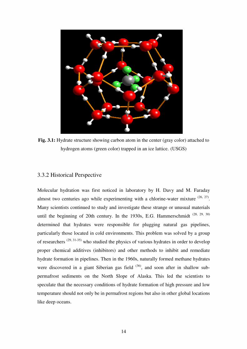
3.3.2 Historical Perspective

Molecular hydration was first noticed in laboratory by H. Davy and M. Faraday

almost two centuries ago while experimenting with a chlorine-water mixture (26, 27)

.

Many scientists continued to study and investigate these strange or unusual materials

until the beginning of 20th century. In the 1930s, E.G. Hammerschmidt (28, 29, 30)

determined that hydrates were responsible for plugging natural gas pipelines,

particularly those located in cold environments. This problem was solved by a group

of researchers (29, 31-35)

who studied the physics of various hydrates in order to develop

proper chemical additives (inhibitors) and other methods to inhibit and remediate

hydrate formation in pipelines. Then in the 1960s, naturally formed methane hydrates

were discovered in a giant Siberian gas field (36)

, and soon after in shallow sub-

permafrost sediments on the North Slope of Alaska. This led the scientists to

speculate that the necessary conditions of hydrate formation of high pressure and low

temperature should not only be in permafrost regions but also in other global locations

like deep oceans.

15

The new discovery also encouraged the scientists to continue their investigation on

hydrates, which was then intensified, expanded, and spread out to cover different

types of hydrates along with the newly and continuously developed spectroscopic

techniques. In the massively increasing number of reports, the scientists concentrated

on studying different aspects of these compounds like physical and chemical

properties, formation and decomposition, structure, global distribution, locations and

stability, concentration, and the true energy potential of natural hydrates. Such

information is necessary to develop computer models that can accurately predict the

behavior of hydrates and hydrate-sediment systems under changing conditions. It can

be also a build up foundation of basic knowledge for methane hydrates and other

types of hydrates.

The occurrence of natural methane hydrates has also promoted many countries to

launch different research projects around the globe looking for all possible locations

on earth that have environmental conditions of high pressure and low temperature for

natural hydrates formation.

16

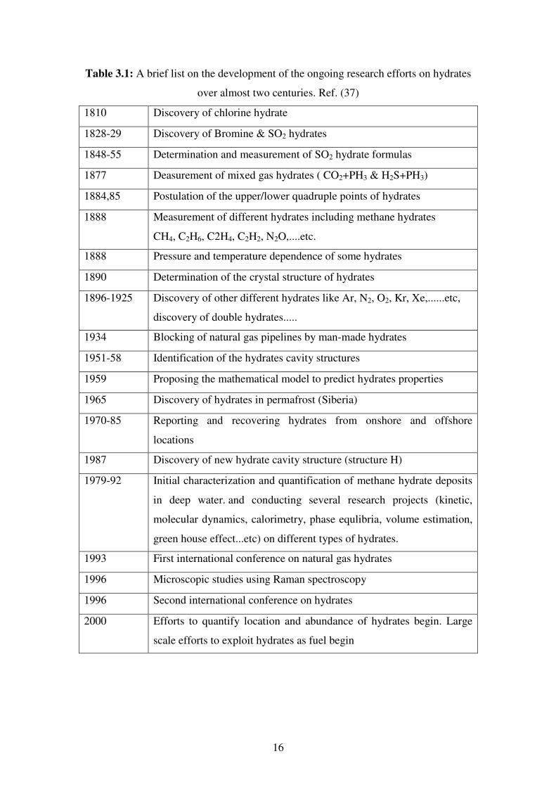
Table 3.1: A brief list on the development of the ongoing research efforts on hydrates

over almost two centuries. Ref. (37)

1810 Discovery of chlorine hydrate

1828-29 Discovery of Bromine & SO2 hydrates

1848-55 Determination and measurement of SO2 hydrate formulas

1877 Deasurement of mixed gas hydrates ( CO2+PH3 & H2S+PH3)

1884,85 Postulation of the upper/lower quadruple points of hydrates

1888 Measurement of different hydrates including methane hydrates

CH4, C2H6, C2H4, C2H2, N2O,....etc.

1888 Pressure and temperature dependence of some hydrates

1890 Determination of the crystal structure of hydrates

1896-1925

Discovery of other different hydrates like Ar, N2, O2, Kr, Xe,......etc,

discovery of double hydrates.....

1934 Blocking of natural gas pipelines by man-made hydrates

1951-58 Identification of the hydrates cavity structures

1959 Proposing the mathematical model to predict hydrates properties

1965 Discovery of hydrates in permafrost (Siberia)

1970-85 Reporting and recovering hydrates from onshore and offshore

locations

1987 Discovery of new hydrate cavity structure (structure H)

1979-92

Initial characterization and quantification of methane hydrate deposits

in deep water. and conducting several research projects (kinetic,

molecular dynamics, calorimetry, phase equlibria, volume estimation,

green house effect...etc) on different types of hydrates.

1993 First international conference on natural gas hydrates

1996 Microscopic studies using Raman spectroscopy

1996 Second international conference on hydrates

2000

Efforts to quantify location and abundance of hydrates begin. Large

scale efforts to exploit hydrates as fuel begin

17

3.3.3 Crystal structure

X-ray diffraction technique has been extensively used to study the crystal structure of

hydrates by Von Stakelberg and coworkers in 1950s (38 - 49)

. The analysis of their

efforts led to the determination of the first two types of crystal structure of hydrates

known as structure I and structure II. These structures represent different

arrangements of water molecules resulting in slightly different shapes, sizes, and

assortments of cavities. The structure formation depends on various aspects of the

available guest molecule. Both structures I and II can be stabilized by filling at least

70 percent of the cavities by a single guest molecule, therefore known as simple

hydrates.

In 1987 Ripmeister and others (50 - 54)

discovered a third type of hydrate structure

named as structure H which requires the cooperation of two guest molecules (one

large and one small) to stabilize, thus known as double hydrate. Structure H hydrates

are rare, but are known to exist in locations where a thermogenic production of heavy

hydrocarbons is common.

The continuous experimental advances and developments in this field may result in

discovering more exotic and complex structures of gas hydrates. Methane is

commonly the dominant component of clathrate gas hydrates formed either in nature

or in industrial processes. Due to its small molecular size, methane can serve as a

guest molecule in all the three known gas hydrate structures I, II, and H.

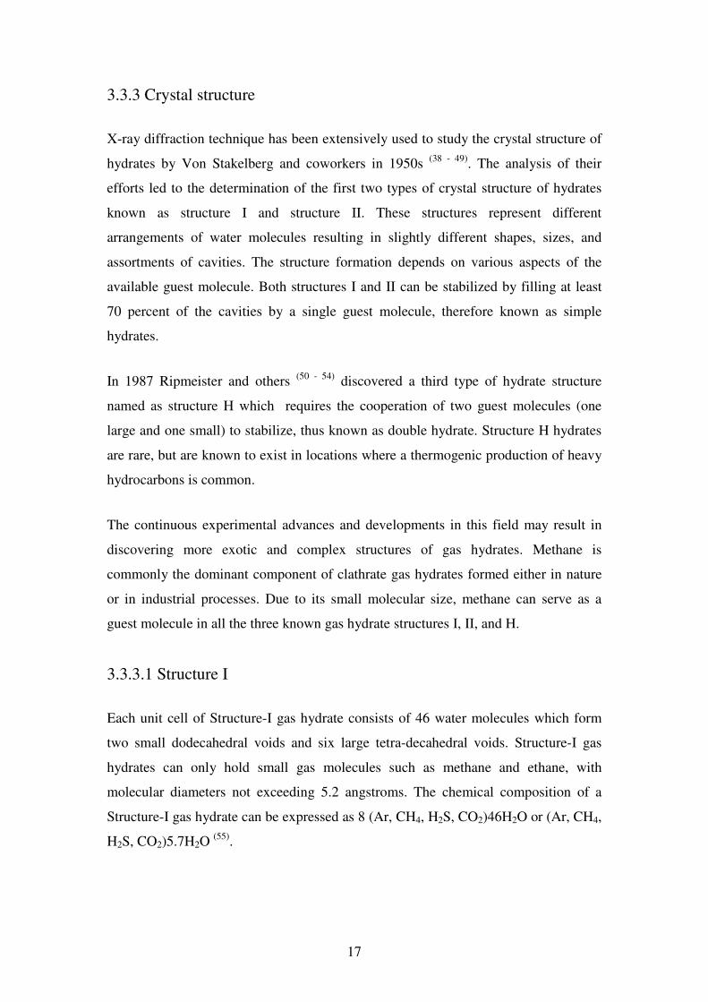
3.3.3.1 Structure I

Each unit cell of Structure-I gas hydrate consists of 46 water molecules which form

two small dodecahedral voids and six large tetra-decahedral voids. Structure-I gas

hydrates can only hold small gas molecules such as methane and ethane, with

molecular diameters not exceeding 5.2 angstroms. The chemical composition of a

Structure-I gas hydrate can be expressed as 8 (Ar, CH4, H2S, CO2)46H2O or (Ar, CH4,

H2S, CO2)5.7H2O (55)

.

18

512

512

62

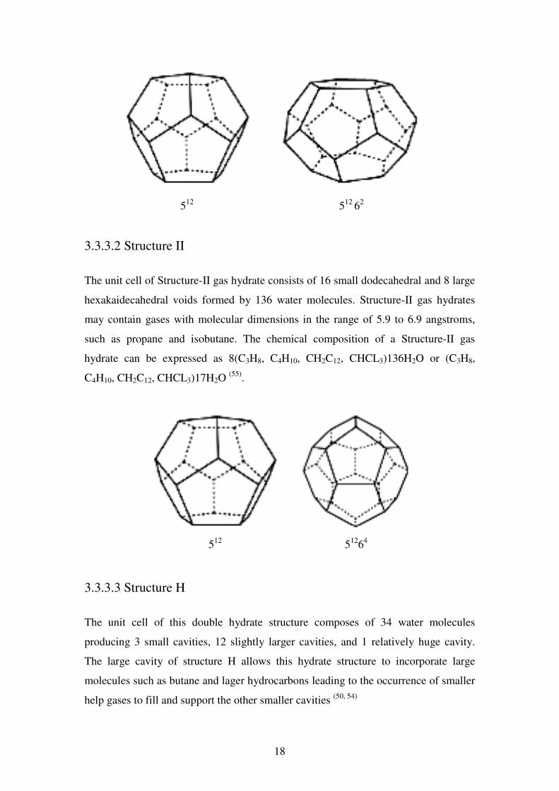
3.3.3.2 Structure II

The unit cell of Structure-II gas hydrate consists of 16 small dodecahedral and 8 large

hexakaidecahedral voids formed by 136 water molecules. Structure-II gas hydrates

may contain gases with molecular dimensions in the range of 5.9 to 6.9 angstroms,

such as propane and isobutane. The chemical composition of a Structure-II gas

hydrate can be expressed as 8(C3H8, C4H10, CH2C12, CHCL3)136H2O or (C3H8,

C4H10, CH2C12, CHCL3)17H2O (55)

.

512

512

64

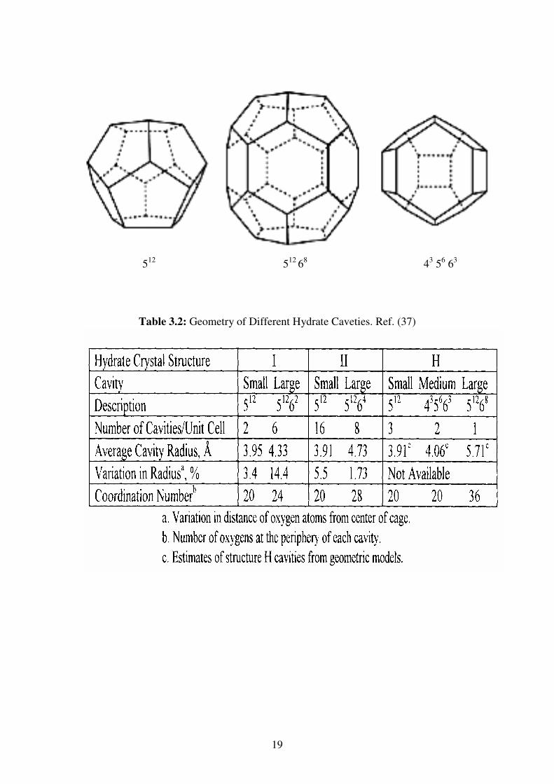
3.3.3.3 Structure H

The unit cell of this double hydrate structure composes of 34 water molecules

producing 3 small cavities, 12 slightly larger cavities, and 1 relatively huge cavity.

The large cavity of structure H allows this hydrate structure to incorporate large

molecules such as butane and lager hydrocarbons leading to the occurrence of smaller

help gases to fill and support the other smaller cavities (50, 54)

19

512

512

68 4

3 5

6 6

3

Table 3.2: Geometry of Different Hydrate Caveties. Ref. (37)

20

3.3.4 Phase equilibrium Stability

In general, a combination of low temperature and high pressure is needed to support

methane hydrate formation. In addition to temperature and pressure, the composition

of both the water and the gas are also critical for the fine tuning of gas hydrates

stability, i.e. the type of the used water and natural gas in the experiment (56)

.

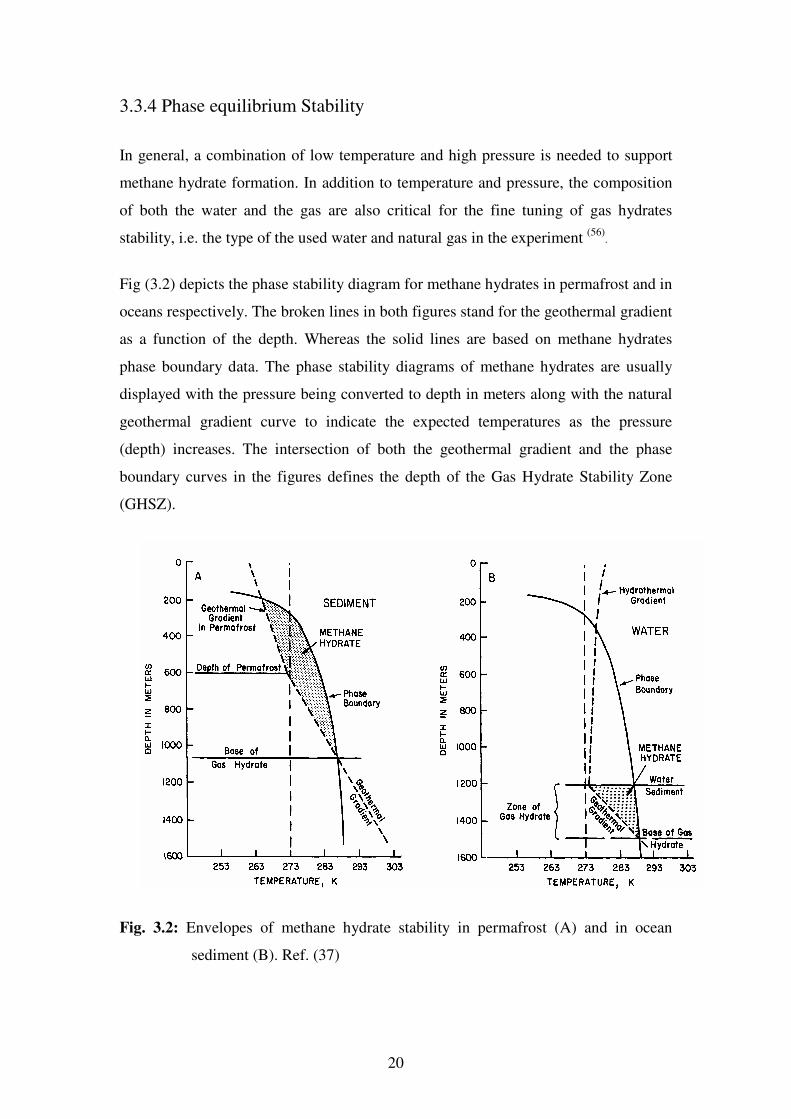
Fig (3.2) depicts the phase stability diagram for methane hydrates in permafrost and in

oceans respectively. The broken lines in both figures stand for the geothermal gradient

as a function of the depth. Whereas the solid lines are based on methane hydrates

phase boundary data. The phase stability diagrams of methane hydrates are usually

displayed with the pressure being converted to depth in meters along with the natural

geothermal gradient curve to indicate the expected temperatures as the pressure

(depth) increases. The intersection of both the geothermal gradient and the phase

boundary curves in the figures defines the depth of the Gas Hydrate Stability Zone

(GHSZ).

Fig. 3.2: Envelopes of methane hydrate stability in permafrost (A) and in ocean

sediment (B). Ref. (37)

21

In fig (3.2-A), the phase diagram shows typical conditions in a permafrost region of

the North Pole assuming a permafrost depth of 600 meters. The overlap of both the

phase boundary and temperature gradient curves indicates that the GHSZ should

extend from a depth of about 200 meters to slightly more than 1,000 meters, i.e. when

hydrates are initiated, more nucleation can occur with increasing pressure or

decreasing temperature.

Figure (3.2-B) shows the phase diagram for a typical location on Deep Ocean. A

seafloor depth of 1200 meters is assumed. The temperature steadily decreases with

increasing depth, reaching down to values close to 0°C at the ocean bottom. As one

goes down below the ocean bottom, the temperatures start to constantly increase

again. These settings imply that the top of the GHSZ occurs at roughly 400 meters

while the base of the GHSZ lies at 1500 meters. Therefore, hydrates will only form in

the sediments within this region. However, at very deep sediments, methane hydrates

are not likely to be formed due to the lack of high biological productivity (the bacteria

which are needed to produce the organic matter that is converted to methane) and

rapid sedimentation rates (to eliminate the organic matter) that support hydrate

formation on the continental shelves (37)

.

3.3.5 Occurrence and Locations (global distribution)

The knowledge of methane hydrates was limited on it’s occurrence in chemical

laboratories and natural gas pipelines. However, a series of discoveries started first at

the North Pole and then spread out to deep water regions of all continents indicated

that natural methane hydrates exist on a huge scale.

The existence of natural methane hydrate in many locations is concluded by using

certain geophysical survey techniques or geochemical analyses of sediment samples.

However, the number of locations is continuously increasing where more detailed

information is being collected. This wide range of information can ultimately form a

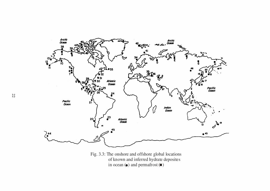
knowledge basis for natural gas hydrates. Fig (3.3) shows both an onshore and

offshore global map for more than 50 sites of methane hydrates which have been

identified by geophysical and geochemical techniques (57, 58)

.

22

Fig. 3.3: The onshore and offshore global locations of known and inferred hydrate deposites in ocean ( ) and permafrost ( )

23

3.3.6 Estimated amount

There is no available data on the absolute amount of methane hydrate in earth, but it is

generally accepted that the global volume of methane in hydrates is immense and far

exceeding the volume of methane in any other form. However, the estimates of

methane volume compressed in hydrates are widely changing among different

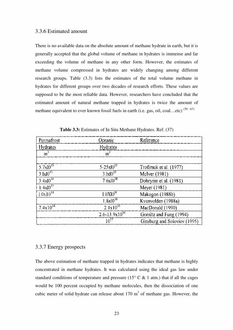
research groups. Table (3.3) lists the estimates of the total volume methane in

hydrates for different groups over two decades of research efforts. These values are

supposed to be the most reliable data. However, researchers have concluded that the

estimated amount of natural methane trapped in hydrates is twice the amount of

methane equivalent to ever known fossil fuels in earth (i.e. gas, oil, coal…etc) (59 - 67)

Table 3.3: Estimates of In Situ Methane Hydrates. Ref. (37)

3.3.7 Energy prospects

The above estimation of methane trapped in hydrates indicates that methane is highly

concentrated in methane hydrates. It was calculated using the ideal gas law under

standard conditions of temperature and pressure (15° C & 1 atm.) that if all the cages

would be 100 percent occupied by methane molecules, then the dissociation of one

cubic meter of solid hydrate can release about 170 m3 of methane gas. However, the

24

maximum occupancy ranges between 70 and 90 percent, therefore one cubic meter of

methane in nature turns out to contain up to 164 m3 of methane. In another reference,

it is stated that each volume of methane hydrates can contain 184 volume of methane.

These figures conclude that methane hydrates are considered as a huge potential

energy source for many applications (57, 58, 63)

.

25

___________________________________________________________________________

CHAPTER 4

Experimental setup and Instrumentation

___________________________________________________________________________

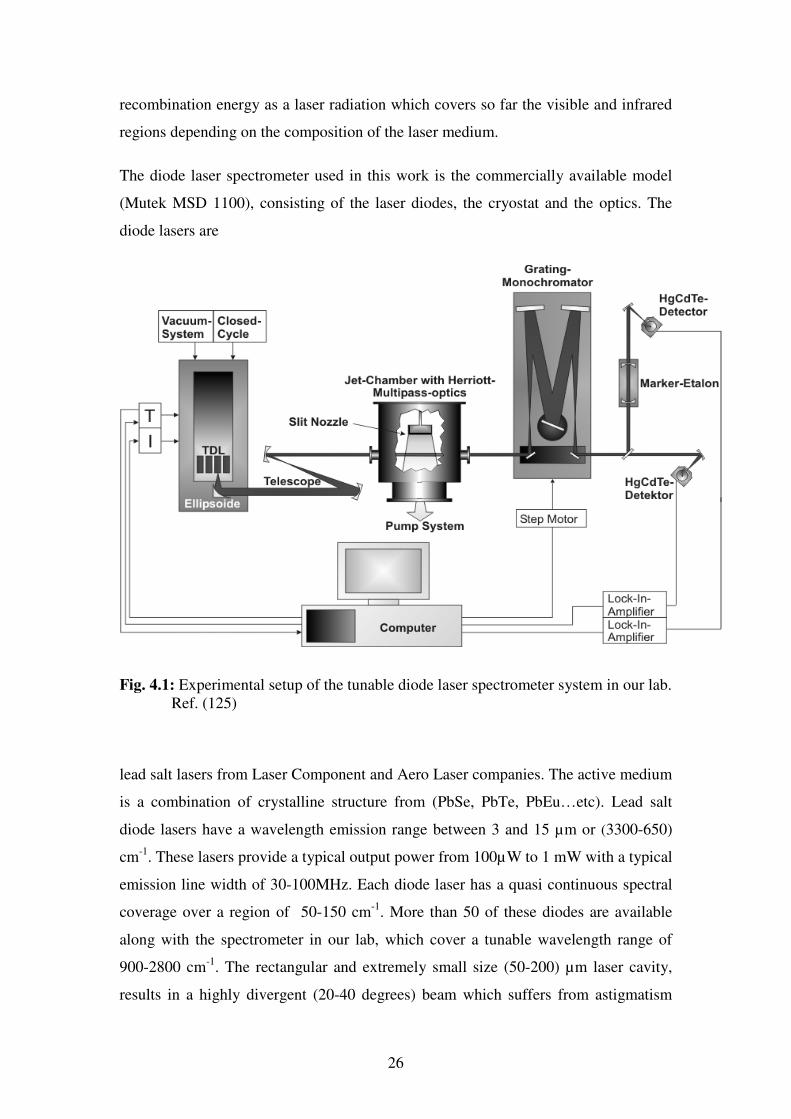
The experimental layout of the computer controlled diode laser spectrometer and the

molecular jet system used in this work is shown in fig. (4.1). This system is used to study

and investigate different species of relatively small and weakly bound molecular

complexes. The setup is constructed of three major parts, the diode laser spectrometer,

the molecular jet and the data acquisition system. A comprehensive introduction on

the tunable diode laser spectroscopy is given in (68-71), and an introduction on the

theory of lead salt diode lasers is also given in (72, 73). The components of

experimental setup will be described briefly in the following sections. More detailed

information about the diode laser spectrometer system can be found in (74).

4.1 The Tunable Diode laser spectrometer

4.1.1 Laser source

Diode lasers are classified as solid state lasers, where the laser or lasing medium is

usually made up of doped solid crystalline materials (e.g.; ruby, Nd-YAG, Nd-Glass,

Nd-YLF, etc). Diode lasers, also called semiconductor lasers, are the smallest ever

made lasers with an active medium of grain size crystal, which is usually cut in a

rectangular shape with cleaved facets to work as the laser resonator. The other facets

are destroyed by using different methods like etching, grounding, ion

implantation....etc. These little tiny crystals are basically a combination of some

doped semiconductor materials or alloys in a p-n junction. The frequency range of a

diode laser is commonly determined by the exact composition of the semiconductor

crystals, which is precisely selected and controlled in the manufacturing phase. The

laser action takes place in these crystals when a voltage is applied on the p-n junction.

Then holes and electrons are generated in the junction, thereby creating a population

inversion within the junction. Electrons and holes then recombine and emit the

26

recombination energy as a laser radiation which covers so far the visible and infrared

regions depending on the composition of the laser medium.

The diode laser spectrometer used in this work is the commercially available model

(Mutek MSD 1100), consisting of the laser diodes, the cryostat and the optics. The

diode lasers are

Fig. 4.1: Experimental setup of the tunable diode laser spectrometer system in our lab.

Ref. (125)

lead salt lasers from Laser Component and Aero Laser companies. The active medium

is a combination of crystalline structure from (PbSe, PbTe, PbEu…etc). Lead salt

diode lasers have a wavelength emission range between 3 and 15 µm or (3300-650)

cm-1

. These lasers provide a typical output power from 100µW to 1 mW with a typical

emission line width of 30-100MHz. Each diode laser has a quasi continuous spectral

coverage over a region of 50-150 cm-1

. More than 50 of these diodes are available

along with the spectrometer in our lab, which cover a tunable wavelength range of

900-2800 cm-1

. The rectangular and extremely small size (50-200) µm laser cavity,

results in a highly divergent (20-40 degrees) beam which suffers from astigmatism

27

and elliptical beam profile. These drawbacks of the laser beam lead to inhomogeneous

broadening of the gain profile which results in multimode laser radiation or emission

across the frequency range of the diode laser. These modes are typically separated by

1 to 4 cm-1

and can be continuously tuned over a frequency range of 0.5 to 2 cm-1

.

Therefore, single mode operation of these lasers is limited to small regions and only

possible in certain cases. In principle, all diode lasers have a similar overall

performance, but each diode laser is a unique device with highly individual

characteristics that depends on the composition of the semiconductor crystal and the

applied current and temperature. Even diode lasers from the same crystal may have

unique beam properties.

The sensitivity of the spectrometer is not limited by the f1 laser noise that shows up

to frequencies of 100MHz, but through etalon structures in the signal. This can be

caused by every pair of reflecting surfaces in the beam path which in our setup are for

example the 12 cm diameter mirrors of the Herriott multi-pass-cell. But the pump

vibrations are transferred to the mirrors of the cell as they are very heavy. These

mirror vibrations destroy the phase coherence of the etalon signals, so that they are

mostly damped and show up rarely. The distinct improvement of the signal-to-noise

ratio is depicted exemplarily in (75).

The wavelength emission of diode lasers is a function of the diode temperature and

the applied current. The coarse tuning is mainly done by varying the diode

temperature, while the fine tuning is achieved by smooth changes of the applied

current; i.e. continuous tuning over a small limited range or across a selected

longitudinal mode. In coarse tuning, the temperature change causes a variation in the

band energy gap and a modification of the cavity length of the diode laser due to the

changing refractive index (n) of the semiconductor crystal. These changes lead to the

so called mode jumping where different modes are generated to fit different cavity

lengths, i.e. one mode is terminated and a second one is generated at another

temperature to fit the new cavity length. The second tuning method of the diode laser

is based on changing the applied current while the temperature being held fixed. This

normally produces a small amount of Joule heating that causes a slight change in the

diode temperature and leads to alteration of the refractive index (n). In this method the

change of refractive index results in a negative tuning rate ∆ν ⁄∆I, while the

28

temperature increase yields a positive tuning rate. However, these changes shift the

laser modes in the same direction as the band gap change, but at a slower rate, thus,

providing a more precisely and controllable way of continuous tuning over limited

ranges, i.e. single mode range. The very short time scale of current tuning ≤ 1µs

compared with the time scale of the temperature tuning 5-30 seconds makes it more

profitable or suitable to use for scanning the diode lasers over their frequency range.

The typical tuning rates are:

Current tuning: ∆ν ⁄ ∆I = 0.2-3 GHz ⁄ mA

Temperature tuning: ∆ν ⁄ ∆T = 10-100 MHz ⁄ mK

4.1.2 Cryostat

Lead salt diode lasers operate at cryogenic temperatures, i.e. < 80 K. A closed-cycle

helium cooler from Leybold is used to cool the laser diodes down to 20 K; it also has

a precise temperature control over the working range of the diode laser between 20

and 70 K. It is a long term, maintenance free system with a water-cooled compressor.

The cryostat is mechanically isolated against the vibration of the helium cooler. Four

different diode lasers can be accommodated and simultaneously cooled down in the

cryostat chamber. The desired temperature of the diode laser is achieved by resistive

heating, i.e. by changing the current through a heating coil plugged to the cold finger

of the copper cold head which hosts the diode lasers. A special temperature controller

with the required accuracy over the whole range (10-200K) was developed in our

group, since such a controller was not commercially available; it utilizes a platinum

resistor (Pt1000) as a temperature sensor which guarantees high stability, absolute

accuracy (± 0.5 K), excellent reproducibility (0.05-0.1 K) and quick response (76)

. The

actual control is achieved by using a precision analog PID (Potential-Integration-

Differential) controller designed also in our group to produces an out put voltage

which drives the heater current of the diode laser. The current can be adjusted

between 0 and 900 mA with smallest step of 0.3 µA.

A set of compensated mirror optics consisting of two ellipsoidal mirrors with foci of

40mm and 140mm, one toroidal mirror with (f = 110mm) and some plane mirrors are

29

used to both select one of the four laser diodes in the cryostat and to collimate the

diffraction broadened laser beam which exits the cryostat via a tilted CaF2 plane

window. The collimated output laser beam is then passed through a telescope

arrangement (two mirrors with f = 60 cm and f = 10 cm) to reduce the beam diameter

from 14 mm to 3mm. This is the optimal beam size required for coupling into the

multi-pass cell located inside the vacuum chamber to exclusively probe the expansion

zone of the slit nozzle. This extends a few cm vertical to the expansion direction,

thereby increasing the signal to noise ratio. Purely reflective optical elements are used

in the optical path of the laser beam in order to minimize the feedback to the diode

lasers. No lenses are used in the optical setup as they act as a source of small back

reflection in the laser cavity. The optimal laser beam is then guided to enter the

vacuum chamber through a CaF2 window, where it is coupled in a Herriott multi-pass

cell. The cell arrangement consists of two spherical gold plated and identical concave

mirrors separated by a distance of their radius of curvature; both mirrors have a

diameter of 12 cm and a focal length of 50 mm. The design is made up to couple the

optical beam into the cell through a hole in the first concave mirror. A correct

alignment of the optical beam in the cell results in an elliptical beam spot pattern on

both mirror surfaces, a maximum number of 40 spots can be achieved between the

two mirrors before the beam emerges out of the same coupling hole as it entered. The

number of spots usually determines the number of the beam reflections within the two

mirrors and also specifies the optical absorption length in the cell which is between 80

and 160 cm for this design. This cell was built and integrated into the apparatus in

context of a research Master degree project done in our research group (77)

. This

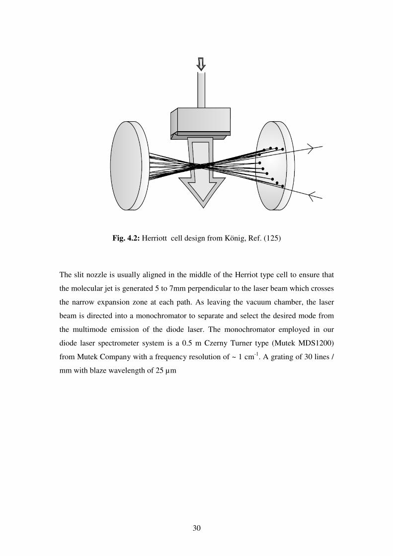
design enables all reflections of the ellipse to be utilized, whereas in the old White

cell design developed by König (70)

, only half of the ellipse could be used as shown in

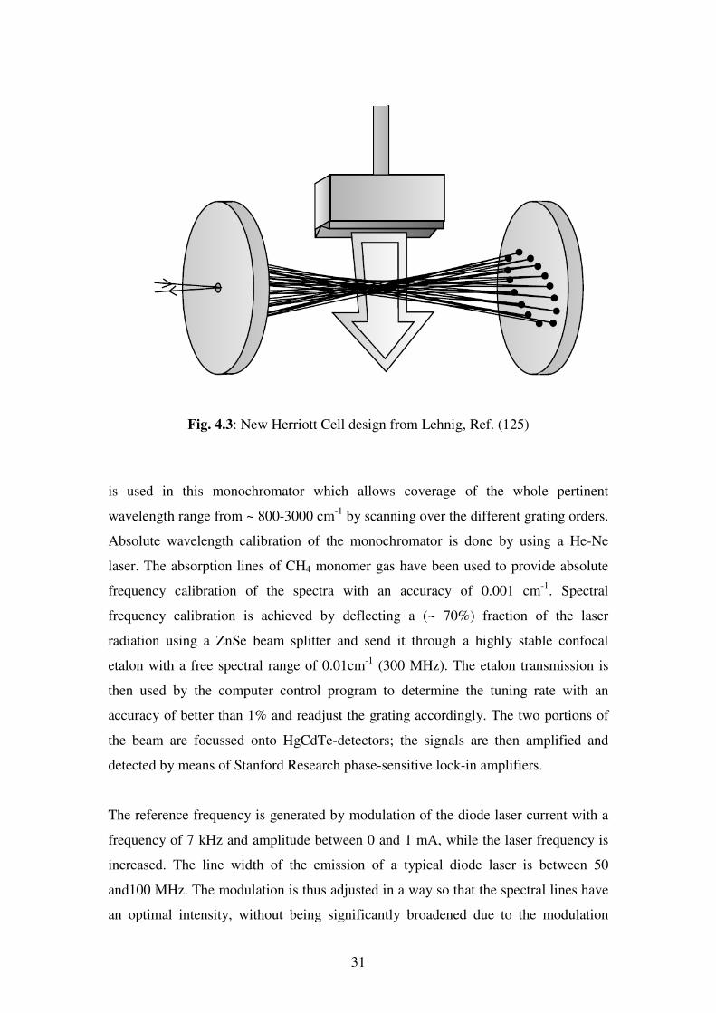
the fig. (4.2). The new cell has brought a further positive aspect for spectroscopy,

apart from the increased number of passes and therefore the increased absorption

length from 80 to 160 cm as shown in fig. (4.3) (77)

.

30

Fig. 4.2: Herriott cell design from König, Ref. (125)

The slit nozzle is usually aligned in the middle of the Herriot type cell to ensure that

the molecular jet is generated 5 to 7mm perpendicular to the laser beam which crosses

the narrow expansion zone at each path. As leaving the vacuum chamber, the laser

beam is directed into a monochromator to separate and select the desired mode from

the multimode emission of the diode laser. The monochromator employed in our

diode laser spectrometer system is a 0.5 m Czerny Turner type (Mutek MDS1200)

from Mutek Company with a frequency resolution of ~ 1 cm-1

. A grating of 30 lines /

mm with blaze wavelength of 25 µm

31

Fig. 4.3: New Herriott Cell design from Lehnig, Ref. (125)

is used in this monochromator which allows coverage of the whole pertinent

wavelength range from ~ 800-3000 cm-1

by scanning over the different grating orders.

Absolute wavelength calibration of the monochromator is done by using a He-Ne

laser. The absorption lines of CH4 monomer gas have been used to provide absolute

frequency calibration of the spectra with an accuracy of 0.001 cm-1

. Spectral

frequency calibration is achieved by deflecting a (~ 70%) fraction of the laser

radiation using a ZnSe beam splitter and send it through a highly stable confocal

etalon with a free spectral range of 0.01cm-1

(300 MHz). The etalon transmission is

then used by the computer control program to determine the tuning rate with an

accuracy of better than 1% and readjust the grating accordingly. The two portions of

the beam are focussed onto HgCdTe-detectors; the signals are then amplified and

detected by means of Stanford Research phase-sensitive lock-in amplifiers.

The reference frequency is generated by modulation of the diode laser current with a

frequency of 7 kHz and amplitude between 0 and 1 mA, while the laser frequency is

increased. The line width of the emission of a typical diode laser is between 50

and100 MHz. The modulation is thus adjusted in a way so that the spectral lines have

an optimal intensity, without being significantly broadened due to the modulation

32

frequency. As a result of frequency modulation of the diode laser, one obtains a 1f

derivative of the line profile, after demodulation in the lock-in amplifier. In order to

avoid the difficulty of the frequency determination of the spectral lines by certain

fluctuations of the central point of this derivative, one should take the second

harmonic of the demodulated signal at 14 kHz. This procedure will differentiate the

signal once again, so that the line frequency corresponds to the maximum of the line-

shape once more. This new differentiation of the signal also suppresses background

fluctuations with small gradients efficiently. The calculated line widths using the

second harmonic, depending on the modulation, lie in the region of 30-100 MHz.

Despite the fact that absorption spectroscopy is a relatively simple technique,

sensitivities of as low as ∆I/I = 10-5

– 10-6

can be achieved (78, 79)

.

The spectrometer is controlled by means of a computer, programmed with LabVIEW

(71), which also enables, besides the spectroscopic measurements, a characterization of

the laser diode by measurement of the mode chart.

4.2 Supersonic Molecular Jet Apparatus

In principle, a large number of vibrational and the associated rotational levels of

atomic and molecular structures are highly populated at room temperature. The

spectroscopy of such systems usually leads to very complex and congested spectra

which can show several hundreds of overlapping lines that are very difficult or even

impossible to resolve and analyze. Therefore, cooling of atoms and molecules has

been a very important issue in spectroscopy for the last few decades. The aim was

always to look for cooling methods that can dramatically decrease the internal

temperature of the investigated samples. Consequently, very few vibrational and

rotational levels of the ground electronic state of the analyte sample will be populated,

which in turn leads to significantly simplified spectra that are possible to resolve and

analyze. Different types of cooling methods have been developed and used in order to

achieve very low sample temperatures: One method is to cool down the gas in the

spectroscopic cell by surrounding it with liquids at low temperature (e.g. liquid

nitrogen), but this can cause a rapid decrease in the vapour pressure to be too low for

use. The other method is the cryogenic cooling equipments which are very bulky and

expensive to use. A third method is the so-called supersonic jet molecular beam

33

source (supersonic jet expansion technique) that was first described and introduced by

Kantrowitz and Grey in 1951 (80)

. This type of beam source results in remarkably

higher sample density (~ 75 times) than effusive beam sources that were used to

produce atomic and molecular beams as a sample source in various experiments since

the 1920's (81-83)

. These sources played a key roll in the field of chemical physics for

many years (84-86)

. A good description of the early history and development of

supersonic nozzle beams is given by Anderson (87-89)

.

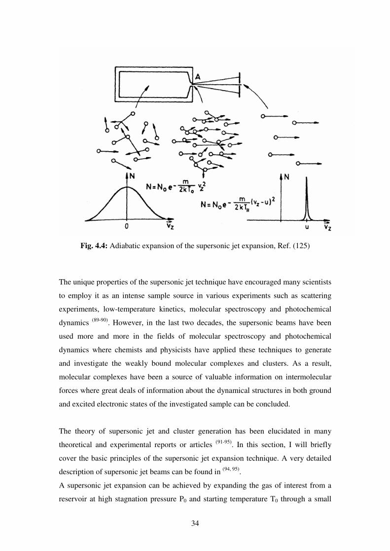
The supersonic jet expansion is a beam source of collision-free atoms and molecules

which are characterized by a very narrow velocity distribution due to negligible

Doppler width and by extremely low translational, vibrational and rotational

temperatures. The rotational temperature can reach down to 1 K while keeping the

sample in the gas phase Fig (4.4). The supersonic jet expansion can as well be used to

intensely produce exotic and transient species (complexes) that normally don't exist at

room temperature. At the primary jet expansion, many complexes or clusters are

formed. As a result of the extremely cold sample beam, the weakly-bound molecular

species such as hydrogen-bonded complexes, Van der Waal complexes or metal

clusters don't decompose due to their very weak binding energies (10-100) cm-1

and

the collision-free condition. Unstable species such as free radicals and ions can also

be produced by the supersonic expansion technique.

34

Fig. 4.4: Adiabatic expansion of the supersonic jet expansion, Ref. (125)

The unique properties of the supersonic jet technique have encouraged many scientists

to employ it as an intense sample source in various experiments such as scattering

experiments, low-temperature kinetics, molecular spectroscopy and photochemical

dynamics (89-90)

. However, in the last two decades, the supersonic beams have been

used more and more in the fields of molecular spectroscopy and photochemical

dynamics where chemists and physicists have applied these techniques to generate

and investigate the weakly bound molecular complexes and clusters. As a result,

molecular complexes have been a source of valuable information on intermolecular

forces where great deals of information about the dynamical structures in both ground

and excited electronic states of the investigated sample can be concluded.

The theory of supersonic jet and cluster generation has been elucidated in many

theoretical and experimental reports or articles (91-95)

. In this section, I will briefly

cover the basic principles of the supersonic jet expansion technique. A very detailed

description of supersonic jet beams can be found in (94, 95)

.

A supersonic jet expansion can be achieved by expanding the gas of interest from a

reservoir at high stagnation pressure P0 and starting temperature T0 through a small

35

orifice or nozzle with diameter greater than the mean free path into a chamber at much

lower back ground pressure Pb. The chamber is usually evacuated either by a

mechanical or oil diffusion pump to keep the background pressure at Pb. A schematic

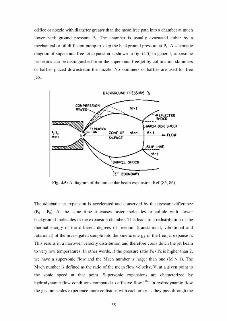
diagram of supersonic free jet expansion is shown in fig. (4.5) In general, supersonic

jet beams can be distinguished from the supersonic free jet by collimation skimmers

or baffles placed downstream the nozzle. No skimmers or baffles are used for free

jets.

Fig. 4.5: A diagram of the molecular beam expansion. Ref (85, 86)

The adiabatic jet expansion is accelerated and conserved by the pressure difference

(P0 - Pb). At the same time it causes faster molecules to collide with slower

background molecules in the expansion chamber. This leads to a redistribution of the

thermal energy of the different degrees of freedom (translational, vibrational and

rotational) of the investigated sample into the kinetic energy of the free jet expansion.

This results in a narrower velocity distribution and therefore cools down the jet beam

to very low temperatures. In other words, if the pressure ratio P0 / Pb is higher than 2,

we have a supersonic flow and the Mach number is larger than one (M > 1). The

Mach number is defined as the ratio of the mean flow velocity, V, at a given point to

the sonic speed at that point. Supersonic expansions are characterized by

hydrodynamic flow conditions compared to effusive flow (96)

. In hydrodynamic flow

the gas molecules experience more collisions with each other as they pass through the

36

nozzle and at some distance downstream; whereas atoms or molecules don’t likely

experience collisions with each others in effusive flow. The conditions are well

described by the Knudsen number

D

Kf

n

λ= (4.1)

Where λf is the mean free path of the molecules in the reservoir and D is the nozzle

diameter. The situation is evaluated as either Kn >> 1 for effusive flow where atoms

or molecules don’t interact, or Kn << 1 for hydrodynamic flow where sample particles

have higher collision rate. In this case the sample particles are more concentrated

about the jet axis and therefore the beam source produces much higher flux. Another

important aspect of supersonic flow is that as a result of nonzero background pressure

in the chamber and as the expansion proceeds in the chamber, the adiabatic expansion

pushes on the gas in the chamber which results in standing shock waves that enclose

the jet expansion to satisfy the boundary conditions exposed by the background

pressure: A symmetric shock wave around the jet called a barrel shock and a disk

shape shock wave far downstream called Mach disc as shown in the figure. The

higher the ratio of P0 / Pb the longer is the distance will be from the nozzle and the

Mach disk. In this case, the supersonic expansion is unable to sense the downstream

boundary conditions and the system of shock waves at the free-jet boundary

conditions compress the gas in the chamber creating regions of high density, pressure,

temperature, and velocity gradients to meet the boundary conditions. The expansion

core is not affected by any external conditions hence the flow is isentropic and is

independent of the background pressure Pb, this region is then called the zone of

silence. At this distance, the regions of high density, pressure, temperature, and

velocity gradients cause numerous collisions between atoms and molecules which

lead to change of flow direction, reduction of Mach number and hence thermalization

of the beam, i.e. the beam is no longer cold and the clusters are destroyed. Therefore,

the measurements should be always taken at few millimetres from the nozzle, or

within the isentropic expansion area (97, 98)

enclosed by the shock waves (zone of

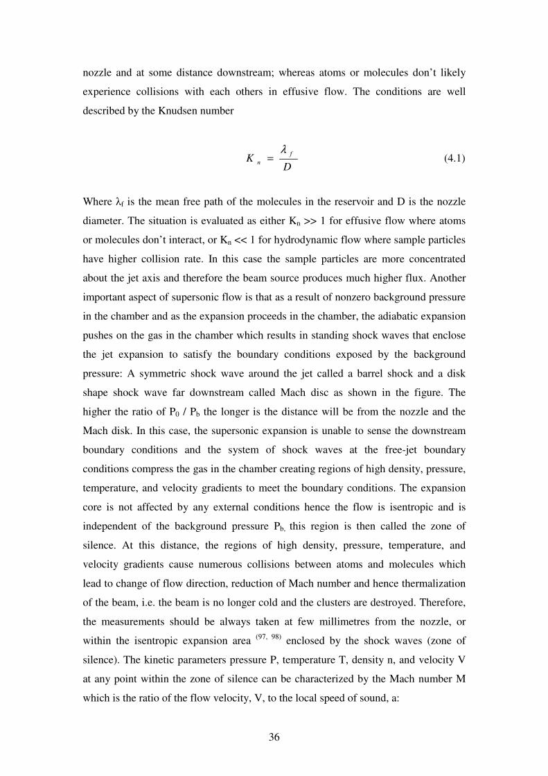
silence). The kinetic parameters pressure P, temperature T, density n, and velocity V

at any point within the zone of silence can be characterized by the Mach number M

which is the ratio of the flow velocity, V, to the local speed of sound, a:

37

a

VM = , WRTa /γ= (4.2)

Where γ = Cp / Cv is the heat capacity ratio of the gas, R is the gas constant and W is

the molecular weight.

The mean flow velocity V can be calculated by using the conservation of energy as

)(22 0

20

TTCdTCV p

T

T

p −== ∫ (4.3)

Therefore, the maximum velocity is given as

)1(/22 00max −== γγ WTRTCV p (4.4)

Where Cp is the heat capacity of the gas

The above equations can be used to calculate the dependency of kinetic parameters, P,

T, and n relative to the stagnation conditions, Po, To, and no, on the Mach number as

follows:

[ ] 12

)1(

0

/)1(

00

2/)1(1−

−−

−+=

=

= M

n

n

P

P

T

Tγ

γγγ

(4.5)

The above equations implies that the flow velocity increases very rapidly with the

Mach number M and then approaches a constant value Vmax compared to the terminal

Mach number Mt where the jet beam gets weaker and the flow is no longer

hydrodynamic. In contrast, the other parameters P, T, N will continue to decrease with

increasing Mach number (91)

.

The Mach number for the regions around the jet axis is given by Levy (98)

as

)1()/( −= γDXAM (4.6)

Where A is constant, X is the distance from the nozzle, and D is the nozzle diameter.

38

The Mach number does not increase with X/D far from the nozzle because the jet gets

weaker and the flow will not be hydrodynamic at long distance from the nozzle and M

will approach a finite terminal value called terminal Mach number Mt.

The Mach disc location can also be calculated in terms of nozzle diameter D by

2/1

0 )/(67.0 bm PPDX = (4.7)

The production of weakly bound complexes is a many body process, i.e. a third

collision partner is needed to form the cluster or molecular complex (dimer, trimer,

etc) and to carry away the excess energy. The collision partner can be either a third

molecule or the nozzle wall. However, the amount of kinetic energy resulting from

complex formation heats up the jet beam again and therefore reduces the adiabatic

cooling in the jet. To overcome this problem as much as possible, the gas from which

the complex is formed can be mixed with a high proportion of either a noble gas ( Ar,

He, Kr,…etc). Helium is found to be the optimum gas for this purpose, because of the

extremely low formation energy of (He)2 which is ≈ 0.0007(2) cm-1

that cannot be

achieved in the jet1. But unfortunately as helium is poorly pumped out by the attached

pumps to the jet beam apparatus, a large background pressure is created in the vacuum

chamber. In order to avoid this problem, and the high cost, argon is usually used as

“carrier-gas” in the molecular jet system.

To achieve the lowest possible background pressure in the vacuum chamber, in spite

of the large gas volume, it is continuously pumped by means of a “three-step” pump-

system, which consists of an Edwards 2600EH-“Root” pump with pump capacity of

2600 m3/h, a Leybold Ruvac 501-“Root” pump with pump capacity 500 m

3/h and a

Leybold S65B pump with pump capacity 65 m3/h. Therefore the background pressure

in the vacuum chamber can be kept within the lower 10-1

mbar region during the

measurements, as long as the stagnation pressure in front of the nozzle does not

exceed 1 bar.

____________________________________________________________________________________________

[1 The depth of the (He)2 potential well measures 7.60(4) cm-1; however the first and only bound state is just

0.0007 cm-1 beneath the dissociation barrier.]

39

4.2.1 Types of Expansions

Two types of nozzles are used in the course of this work; the continuous and the

pulsed slit supersonic nozzles. A short introduction describing these two nozzle types

along with brief introduction on point nozzles will be presented in the following

section.

Pulsed supersonic jets are typically generated from circular (pinhole) nozzles which

produce an axially symmetric expansion, also called point nozzles. The first pulsed

nozzles used in IR-Spectroscopy were “point” nozzles, whose early development is

described by Gentry (100)

. The predominantly employed construction consisted of a

commercial magnetic valve with an aperture ranging from a few tens to several 100

µm in diameter. This allowed pulse lengths of 200-500 µs and modulation frequencies

of up to several kHz to be reached.

Expansions from slit nozzles are known as planar expansions which can be either

continuous or pulse slit nozzles. Normally, the slit has a certain width (d) that can be

also adjustable and infinitely long. However, the length of continuous slits is limited

(4-7) cm, in order to reduce the gas load on the vacuum pumps. The continuous slit

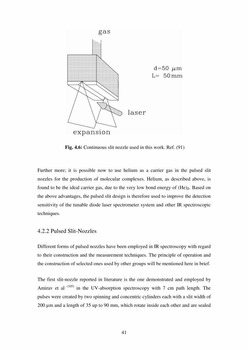
nozzle used in this work is shown in fig. (4.6); the slit length is 5 cm with a typical

width of 50-100 µm. Both pinhole and slit nozzle geometries are commonly used in

spectroscopy, with the slit nozzles having better expansion properties over point

nozzles for several reasons. First, the expansion density falls off as 1/D for slit nozzles

(D is the distance from the nozzle) compared to 1/D2 for point nozzles and thus yields

slower adiabatic cooling. In addition to slower cooling, the slit expansion provides a

higher molecular density per quantum state in the interaction region which increases

the total number of two and three body collisions and therefore greatly enhances the

weakly bound cluster formation. Second, the translational cooling of the slit design

results in a higher collimation of the jet beam (lower velocity spread or small velocity

dispersion) along the slit axes leading to reduced Doppler broadening of the observed

spectral lines i.e. higher experimental resolution. Third, the absorption path length is

much larger in the slit geometry as compared to the point nozzles (101, 102)

.

The supersonic pulsed slit design is the other type of the planar expansion geometries.

The development of both continuous and pulsed planar expansions has been of great

40

importance in spectroscopy, especially in IR spectroscopy, where many weakly bound

complexes have been thoroughly investigated (103, 104)

. The pulsed slit design is of

particular relevance as compared to continuous slit nozzles. The use of a pulsed slit

nozzle reduces the gas flow in the vacuum chamber as a result of low duty cycle2,

while keeping the same level of background pressure as would result from the use of

the continuous nozzle, but at much higher stagnation pressures in front of the nozzle

using the same pump capacity. The high ratio of stagnation pressure to the

background pressure in the pulsed slit expansion design is of twofold advantage. First,

it produces higher beam densities and therefore increases the rate of two and three

body collisions in the interaction region of the jet expansion which consequently

enhances the production of molecular complexes. Second, it also causes a definite

decrease in the translational temperature of sample gas in the jet expansion leading to

significantly simplified spectra as a result of the low number of populated energy

levels. The absorption path length can be further increased by using the pulsed slit

expansions, e.g. the slit length of the continuous nozzle used in this work was fixed to

5 cm in order to avoid unacceptable increase in the background pressure in the

vacuum chamber when using longer slits, while for lower gas consumption much

longer slits can be used. The pulsed slit nozzle used in this work has a slit length of

11.4 cm. This shows that the absorption length is more than doubled as compared to

the continuous slit nozzle which improves the signal to noise ratio.

_______________________________________________________________________________________________________

2 Duty cycle is defined as the ratio of the opening duration of the nozzle to the total measurement time.

41

Fig. 4.6: Continuous slit nozzle used in this work. Ref. (91)

Further more; it is possible now to use helium as a carrier gas in the pulsed slit

nozzles for the production of molecular complexes. Helium, as described above, is

found to be the ideal carrier gas, due to the very low bond energy of (He)2. Based on

the above advantages, the pulsed slit design is therefore used to improve the detection

sensitivity of the tunable diode laser spectrometer system and other IR spectroscopic

techniques.

4.2.2 Pulsed Slit-Nozzles

Different forms of pulsed nozzles have been employed in IR spectroscopy with regard

to their construction and the measurement techniques. The principle of operation and

the construction of selected ones used by other groups will be mentioned here in brief.

The first slit-nozzle reported in literature is the one demonstrated and employed by

Amirav et al (105)

in the UV-absorption spectroscopy with 7 cm path length. The

pulses were created by two spinning and concentric cylinders each with a slit width of

200 µm and a length of 35 up to 90 mm, which rotate inside each other and are sealed

42

up against each other. This enabled a repetition rate of 12 Hz and pulse durations of

150 µs to be obtained.

A pulsed slit-nozzle from Lovejoy and Nesbitt was constructed and used to produce

Van der Waals and hydrogen bonded complexes (106)

. They used a slit length of 1.2

cm with 75 or 125 µm width designed within the nozzle holder with a knife-edge end

projecting on the back side and a mount for interchangeable cutting edge slit nozzles

(blades) on the front side. An elastomer3 seal connected to the solenoid actuator

through a small rod is placed on the knife-edge end of the nozzle holder by a leaf

spring. The valve operates by rapidly pushing and lifting the seal assembly against the

slot of nozzle holder through the applied voltage. A pulse length of 150-600 µs and

repetition rates of up to 60 Hz were achieved with this valve design. A very similar

design was employed by Sharpe et al (107)

and Piante et al (108)

.

Further nozzles can be utilized to increase the absorption path length. The nozzle

holder has then to be modified in order to host the new additional valves. In the design

of Liu et al, three commercially modified and synchronously triggered solenoid valves

from General valve corporation, Series 9 have been employed as shown in fig.

(4.7)(109)

. The use of three valves guarantees a fast homogenous distribution of the jet

gas expansion in front of the slit. This design enables us to increase the slit length to

more than 10 cm. The slit dimensions in Liu et al design is101.6 x 0.127 mm2 with

pulse durations of 0.5-1 ms and a repetition rate up to 80 Hz. Hu et al employed a slit

nozzle of 12 cm x 100 µm with pulse duration of 2ms and a frequency of 3 Hz (110)

.

Both nozzles are adapted to heat them up to 230 C which gives the chance to study

and investigate non-volatile substances like nucleotide basis under standard

conditions. However, a continuous operation with free maintenance for these valves is

only possible for about a 12 hour period

3 In most constructions, it consisted of an o-ring, which was cut open.

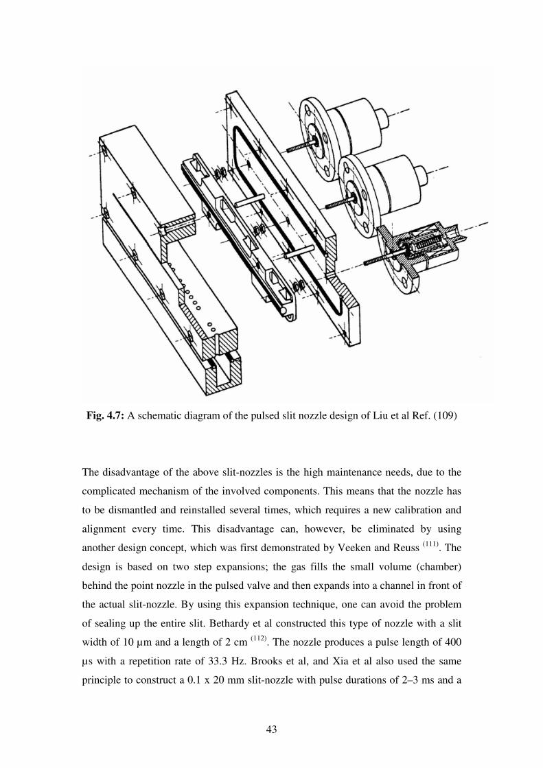
43

Fig. 4.7: A schematic diagram of the pulsed slit nozzle design of Liu et al Ref. (109)

The disadvantage of the above slit-nozzles is the high maintenance needs, due to the

complicated mechanism of the involved components. This means that the nozzle has

to be dismantled and reinstalled several times, which requires a new calibration and

alignment every time. This disadvantage can, however, be eliminated by using

another design concept, which was first demonstrated by Veeken and Reuss (111)

. The

design is based on two step expansions; the gas fills the small volume (chamber)

behind the point nozzle in the pulsed valve and then expands into a channel in front of

the actual slit-nozzle. By using this expansion technique, one can avoid the problem

of sealing up the entire slit. Bethardy et al constructed this type of nozzle with a slit

width of 10 µm and a length of 2 cm (112)

. The nozzle produces a pulse length of 400

µs with a repetition rate of 33.3 Hz. Brooks et al, and Xia et al also used the same

principle to construct a 0.1 x 20 mm slit-nozzle with pulse durations of 2–3 ms and a

44

repetition rate of 3 – 4 Hz (113-116)

. Likewise, Pak et al used different dimensions of slit

nozzles with lengths ranging between 7-40 mm and width of 15 µm which produced

pulse durations of 2.0-2.5 ms at a repetition rate of 80 Hz (117)

. The pulse slit nozzle

used in this work is based on the same principle of operation.

4.3 Possible Detection Methods

In the pulsed jet operational mode, the absorption line can be recorded by either a 2f

phase sensitive detection method using lock-in amplifier or by a gated detection

method using a boxcar gate integrator triggered by the jet expansion repetition rate

which has a maximum frequency of 100 Hz. This is the so-called jet modulation

technique or "concentration modulation". The sensitivity of this technique is limited

by the 1/f low frequency excess noise of the TDL caused mainly by mechanical

vibrations from closed cycle helium cooler (cryostat), compressor, pumps and other

sources. The effect of this laser noise will be more pronounced and significant when

the lock-in amplifier triggered by the jet frequencies (~ 100 Hz) is used. The laser

excess noise can be noticeably reduced by using high repetition pulsed valve

producing short duration pulses of few 100 µs. However, these frequencies are still

too small to overcome the detector-preamplifier thermal noise. For this reason, two

different detection methods have been established, using a combination of pulsed slit-

nozzle and tunable diode laser spectrometer, which enables the detection of

absorption signals as small as 10-4

- 10-5

at frequencies of few 10 kHz. These methods

will be introduced in the following

two sections.

4.3.1 The Rapid-Scan Method

This method is commonly used in slit nozzle experiments with low repetition rates of

few hertz and pulse duration in the millisecond range. In this method, a selected

wavelength range (one laser mode) is measured and recorded over the pulse duration

associated with a rapid scan of the laser current. In addition to this open valve

measurement, a second measurement is also recorded with closed valve. Both scans

are then subtracted from each other to scale down the background noise. A high signal

to noise ratio can be achieved if several 100 to several 1000 of the pulses are averaged

45

and added together. De Piante et al demonstrated the use of the rapid-scan method on

the spectra of the Ar-CO-complex (108)

, Sharpe et al (118, 119)

on HX-CO2 and Ar-CO2

and Dutton et al (120)

on CO2-N2O. Hu et al (110)

observed the Van der Waals complex

N2O-Ar using this technique, whilst Brooks et al and Xia et al used this method to

spectroscopically investigate (CO)2,CO-H2O and CO-N2 (113-116)

. The most serious

problem of this method is the temperature drift of the laser frequency. This means that

each individual scan begins at a slightly different frequency, which inevitably leads to

a broadening of the spectral lines as soon as the scans are averaged. To overcome this

problem, Hu et al developed a fast electronics to stabilize the drift in the laser

frequency. The fast electronics work as a feedback circuit to add the change in the

etalon signal due the thermal drift to the laser current as an error signal. Hu et al

developed this laser electronics because the widening of spectral lines started to be

more and more significant after averaging over 1000 scans at a repetition rate of 3 Hz.

This type of averaging needs an exceptional temperature controller cryostat with large

cooling power and a rapid heating system. Such disadvantage does not apply in our

experimental setup because the laser needs a few seconds to return from the end to the

beginning of a mode, during which the temperature stabilizes itself. However, this fact

would limit the highest possible repetition rate significantly. Another disadvantage of

this method is that it only functions with the diodes with single-mode operation,

whereas it is impossible to scan the monochromator over several wave numbers

within a millisecond range. This method also shows more laser intensity fluctuation in

the base line of the spectrum, which makes the use of at least a 12 bit analog-digital-

converter essential in order to achieve the required resolution of the absorption lines.

These disadvantages can be eradicated using the so-called step-scan method, which

was employed for the nozzles used in this work.

4.3.2 The Step-Scan Method

The step-scan procedure is based on increasing the laser current in single steps,

whereas many measurements are taken at every opening and closing time of the

nozzles. The modulation of the laser frequency is kept the same as used in the

continuous slit nozzle which was mentioned in section 4.1. The use of modulation

frequencies in the region of a few 10 kHz effectively reduces the 1/f-laser noise. The

nozzle was operated with opening durations of 2-3 ms and repetition rates of 40 Hz. If

46

the laser frequency is tuned to an absorption line, then the detector signal consists of

two components in addition to the laser modulation frequency, which corresponds to

the addition and difference of the laser modulation and pulse frequencies. A two-step

demodulation process is then required in order to extract the signal components. The

process starts by multiplying the input signal of the lock-in amplifier with the

reference frequency produced by the lock-in amplifier. The resultant signals constitute

the addition and the difference frequencies of the signal components along with the

reference frequency. For example, if the laser modulation frequency lies at 10 kHz

and the pulse frequency at 100 Hz, then the signal in front of the lock-in amplifier

contains frequency components at 9.9, 10 and 10.1 kHz. While in 2f technique the

multiplication produces frequencies of 0, 0.1, 19.9, 20 and 20.1 kHz. In this case,

since the acquired signal is contained in the 100 Hz components, the lock-in amplifier

generates the relevant signal (different from the usual DC components) to work as a

band pass filter. In principle, the lock-in amplifiers direct the multiplied signal to a

low pass filter, which normally damps all AC-components above the threshold value

of some cut-off frequencies in the signal and pass only the lower DC frequency

components. But since this is not desired here, the bandwidth of the low pass filter

which increases with decreasing time constant of the lock-in amplifier, must be set

high enough so that the signal components of the pulse frequency (in the above

example the component at 100 Hz) can pass through the low pass unaltered. This is

the case for time constants smaller than 1ms. In the case of the gated detection method

using boxcar-integrators, one can integrate over two time intervals one before the

pulse and one during the pulse and then average over a certain number of pulses at

each laser frequency. A second lock-in amplifier, which operates with the pulse

frequency as reference frequency, can be used instead of the Boxcar-integrators. This

method was used initially by Sharpe et al in the investigation of the CO2-Ar complex

(107). Quian et al also used it in conjunction with a pulsed point-nozzle to investigate

the (N2O) 2 (121)

and N2O-noble gas complexes (122)

, whereas Pak et al demonstrated

this technique on Ar-CO (123)

and used it to study CH4-Ar and CH2-Kr complexes (117)

.

Qian et al employed both rapid-scan and step-scan methods to investigate N2O-CO

complexes (124)

. The above discussion showed that the step-scan procedure leads to a

better resolution as well as a higher productivity of the spectrometer.

47

4.4 Set-Up and Operation of the Pulsed slit Nozzle

The pulsed slit nozzle used in this work was developed in the framework of an earlier

PhD thesis (125)

carried out in our group and based on the facts mentioned in section

4.2.2. The design is very similar to the one adapted by Pak et al. (117)

. The slit nozzle is

mainly constructed of three point nozzles set next to each other on a stainless steel

block to increase the slit length as shown in fig. (4.8) and fig. (4.9). To do this, three

commercial point-nozzles (Series 9 from the company Parker Hannifin, formerly

General Valve) with an aperture diameter of 800 µm were mounted next to each other

on a stainless steel block.

Three holes of 2mm in diameter are made in the block. These holes are exactly

aligned with the position of the three apertures of the point nozzles on the block to

transport the jet gas into a long channel of 11.4 cm with a cross sectional area of 2 x 2

mm2. Two adjustable stainless steel cutting edge blades are then fixed over this

channel on the bottom of the block; the blades can be adjusted by using a microscope

to form a slit of 50-100 µm along the whole channel on the bottom of the block. In

addition to the above mentioned advantages, this design makes the slit nozzle almost

free of maintenance. Three sealing puppets or plungers have only to be replaced when

they leak out while being in the closing position. The point nozzles are driven by a

commercial pulse driver (IOTA ONE from Parker Hannifin) which can

synchronically trigger up to four valves simultaneously. Pulse durations as low as

microsecond with a repetition rate of up to 50 kHz can be achieved by this driver. The

required pulse parameters for the installed valves (opening and closing time,

triggering mode...etc) are set and executed through the two on-time and off-time

functions within a small window on the front panel of the valve driver. The valve

driver uses these parameters to calculate the frequency to be f = 1/(on-time + off-

time). The set parameters are also used by the valve driver to generate a continuous

series of pulses along with the same number of TTL signals which trigger the data

acquisition inside the PC.

In order to substantially increase the number of the collected data points during one

pulse, a high resolution 8 bit rapid digital-analog converter card (NI 5102 from

National Instruments) with a maximum sampling rate of 20 M sample/s (mega

samples per second) was used. This card replaces the Boxcar-integrators described in

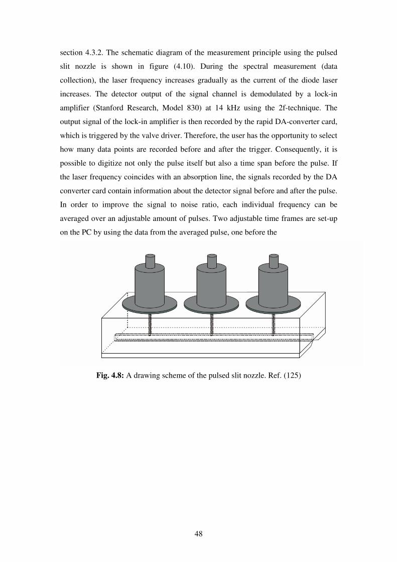
48

section 4.3.2. The schematic diagram of the measurement principle using the pulsed

slit nozzle is shown in figure (4.10). During the spectral measurement (data

collection), the laser frequency increases gradually as the current of the diode laser

increases. The detector output of the signal channel is demodulated by a lock-in

amplifier (Stanford Research, Model 830) at 14 kHz using the 2f-technique. The

output signal of the lock-in amplifier is then recorded by the rapid DA-converter card,

which is triggered by the valve driver. Therefore, the user has the opportunity to select

how many data points are recorded before and after the trigger. Consequently, it is

possible to digitize not only the pulse itself but also a time span before the pulse. If

the laser frequency coincides with an absorption line, the signals recorded by the DA

converter card contain information about the detector signal before and after the pulse.

In order to improve the signal to noise ratio, each individual frequency can be

averaged over an adjustable amount of pulses. Two adjustable time frames are set-up

on the PC by using the data from the averaged pulse, one before the

Fig. 4.8: A drawing scheme of the pulsed slit nozzle. Ref. (125)

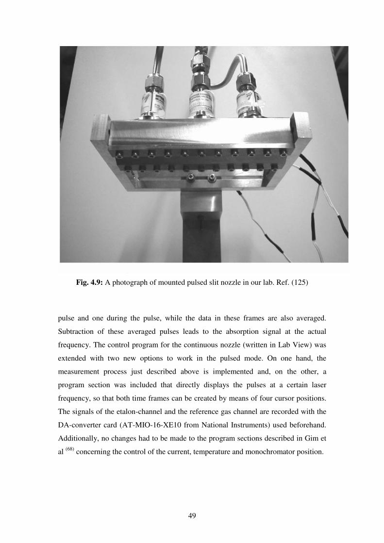
49

Fig. 4.9: A photograph of mounted pulsed slit nozzle in our lab. Ref. (125)

pulse and one during the pulse, while the data in these frames are also averaged.

Subtraction of these averaged pulses leads to the absorption signal at the actual

frequency. The control program for the continuous nozzle (written in Lab View) was

extended with two new options to work in the pulsed mode. On one hand, the

measurement process just described above is implemented and, on the other, a

program section was included that directly displays the pulses at a certain laser

frequency, so that both time frames can be created by means of four cursor positions.

The signals of the etalon-channel and the reference gas channel are recorded with the

DA-converter card (AT-MIO-16-XE10 from National Instruments) used beforehand.

Additionally, no changes had to be made to the program sections described in Gim et

al (68)

concerning the control of the current, temperature and monochromator position.

50

Fig. 4.10: A schematic drawing of the measuring principle with pulsed slit nozzle.

Ref. (125)

51

___________________________________________________

CHAPTER 5

Infrared Spectroscopy of Methane Complexes

___________________________________________________________________________

Spectroscopy has been the most powerful tool to study and investigate the interaction

of electro-magnetic radiation with the three states of matter (gas, liquid and solid) for

more than a century. The interaction can be absorption, emission or scattering of the

electromagnetic radiation by the atoms or molecules of the sample matter. These

interactions lead to different types of spectroscopy that have been classified based on

the spectral region of the electromagnetic radiation i.e. gamma-ray, X-ray, UV, Vis,

microwave, infrared…etc. In absorption spectroscopy, the type of the involved

transition between energy levels in the studied sample can define the frequency range

of the electromagnetic radiation. For example, if the absorption is associated with a

transition from one molecular rotational level to another, then the radiation belongs to

the microwave region of the EM spectrum and the technique is known as microwave

spectroscopy. While in ultraviolet-visible or electronic absorption spectroscopy, the

involved transition takes place among the valence electrons in atoms or molecules.

But if the transition is from one vibrational level to another level, then the radiation

belongs to the infrared region and the technique is called infrared spectroscopy.

Infrared spectroscopy has a long history, but it has been a well established and

effectively used technique since the 1930’s. Infrared spectroscopy is the most

common and popular spectroscopic technique used mainly by chemists to study a

broad band of atomic and molecular species. It yields a great deal of information on

substance and compound identification and the determination of various

characteristics of their structures. The versatility of infrared spectroscopy along with

the development of a wide variety of new laser techniques encouraged the researchers

to use IR spectroscopy to study the molecular complexes produced by supersonic

molecular beam techniques.

52

Early infrared studies of molecular complexes started back in the beginning of the

1980’s where a long path cell cooled down to low temperatures was used (126)

,

whereas the first set of rotationally resolved infrared studies of molecular complexes

in molecular beams appeared in the late 1980’s (127 -131)

.

The Van der Waals molecular complexes have been of considerable interest both

experimentally and theoretically for a long time. Therefore, in the last two decades

this technique (IR) is continued to be used by an increasing number of research

groups to investigate a variety of Van der Waals molecular complexes. The rare-gas

Van der Waals molecular complexes involving symmetric, asymmetric and spherical

top molecules are of great interest in the field of molecular spectroscopy because

these complexes play an important role in understanding the anisotropic behavior of

the Van der Waals interactions. Methane is a spherical top molecule which exists in

huge quantities and different forms on earth; it is also an active constituent of the

atmospheres of earth and the outer planets of the solar system. The methane Van der

Waal complexes have a relatively simple structure. Therefore, the methane related

phenomena can be accurately monitored by studying and investigating the

spectroscopic and collisional processes of all possible methane complexes. These

studies are highly desirable to produce improved models which can be extended to

more complicated molecular systems.

The spectroscopic studies of Van der Waals complexes allows one to determine the

geometrical structure of the complex, the characteristic of the internal motion of the

molecule relative to the atom inside the complex, and to develop an accurate

intermolecular potential energy surface from which various chemical and physical

properties of the molecular system can be extracted. The potential energy surfaces of

these complexes are far from isotropic; i.e. different mutual orientations result in

minima, maxima, saddle points and other features which are essential to their

structural and dynamical properties. Over more than two decades great experimental

and theoretical progress has been made in the understanding of the properties of Van

der Waals complexes. The work on methane Van der Waals complexes started first by

investigating the methane-argon complex using conventional techniques. There has

been a considerable amount of experimental work and measurements on both the bulk

and transport properties of the system (viscosities (132-134)

, diffusion coefficients (135 -

53

137), second virial coefficients

(138 - 145), and thermal diffusion factors

(136, 137, 146 - 150).

These data are not sensitive enough to provide the detailed information of the features

of the multidimensional potential. The data always showed simple isotropic potential.

After the advent of modern spectroscopic techniques a large number of experimental

studies have been devoted to examine the collisional processes involving methane and

argon systems (151-158)

. The experiments were mainly concerned with the studies of

rotational relaxation processes and integral and differential cross sections of rotational

excitation (151, 159)

. In the late seventies Buck et al, (153)

measured the total differential

cross-sections in a crossed molecular beam experiment. The results were used to

develop an empirical potential that showed a cross-sectional rainbow structure

sensitive to the depth of the potential. In another study Nesbitt et al, (160)

measured the

state-to-state integral cross-sections for rotational excitation of CH4 in collision with

Ar atoms using crossed molecular beams. The agreement with the empirical potential

developed by Buck et al is quite reasonable.

The Rg-CH4 complex has also been the subject of several high resolution

spectroscopic studies aiming to provide a better understanding about the nature of

internal motions of methane in the complex (161 - 163)

. The first high resolution studies

are the infrared spectra of Ar-CH4, Kr-CH4 and Ne-CH4 that were recorded by

McKellar et al (161)

using a Fourier transform infrared spectrometer with a long path

glass cell cooled down to low temperatures. Strong transitions correlated to the R(0)

transition of the triply degenerate ν3 stretching vibrational band of the CH4 monomer

were measured for the Ar-CH4 and Kr-CH4, while weak features were observed for

Ne-CH4. Jet spectra for the same spectral region of Ar-CH4 at lower temperature were

also recorded by Lovejoy and Nesbitt et al (163)

using a diode laser spectrometer

system along with supersonic slit expansion. Further lower temperature spectra for

Ar-CH4 were detected by Block and Miller et al (162)

, and Howard with co workers

(164). Although the spectra showed partially resolved rotational structures it was not

possible to securely assign the spectra because of the limited resolution in the

McKellar measurements (0.01 cm-1

) and the line broadening due to the fast

predissociation in the other measurements. However the large spacing between the

sub-bands in the spectra indicated that the methane molecule is freely rotating within

the complex. The spectra were assigned a few years later using an ab initio dynamical

calculation where infrared spectra have been calculated and a potential energy surface

54

has been also developed for this system (165-167)

. The calculated spectra showed a good

qualitative agreement with the recorded ones and contributed in the assignment of the

most other transitions. In more recent spectroscopic studies, the infrared spectra of

Ar-CH4, Kr-CH4 and Ne-CH4 complexes in the 7µm region correlating to the ν4 triply

degenerate bending mode of the methane monomer have been measured by Pak et al

(168-170, 236) using a diode laser spectrometer system. The spectra were later reassigned

as P, Q, and R branches corresponding to the R (0) transition of the methane monomer

employing a model initiated first by Randall et al and developed later by Brook et al

(171) for the Ne-SiH4 complex. A Coriolis term is introduced in the Hamiltonian model

to be able to fit the recoded spectra.

Despite a lot of interest, a limited number of ab initio studies have been reported so

far on Rg-CH4 complexes. In the first study, Fowler et al (172)

calculated the long

range dispersion coefficients of Ar-CH4. In a recent work, Szczesniak et al, (173)

reported a few cuts through the interaction potential of Ar-CH4 using MP2 calculation

methods with a relatively small basis set. The calculation predicted an equilibrium

structure with a face configuration where the rare gas atom sits on one of the C3 axes

of CH4 monomer and approaches the face of the CH4 tetrahedron. The position and

the depth of the minimum were determined to be 7.5 bohr and -113 cm-1

respectively.

They also stated that the minimum is overestimated by 0.5 bohr while the depth is

underestimated by 25% respectively due to the applied low level theory and small

basis set. In the most recent study, Hijmann et al, (174)

employed the symmetry adapted

perturbation theory (SAPT) to compute enough data points on the surface to

determine the ab initio intermolecular potential energy surface of the Ar-CH4

complex. This potential is in a good agreement with the previous theoretical study

(175), it also displays a face configuration but with a well depth of -144.3 cm

-1 and a

position of 7 bohr. The SAPT potential is shown to reproduce most of the

experimentally observed data. It is also used to calculate the IR spectrum which

assisted in assigning most the of other transitions; it is probably the best available

potential for the Ar-CH4 complex.

The methane-water complex (CH4-H2O) is another example of the Van der Waal

methane complexes which has attracted special research interest. The specialty of this

complex comes from the fact that methane hydrates are a combination of a methane

55

molecule locked in a cavity of hydrogen bonded water molecules. Therefore the

ability to develop a modeling technique that can predict the behavior of methane

hydrates would be very important for the development of production and transmission

operation of conventional methane hydrates. On the other hand, a proper

determination of the intermolecular interaction potential of the complex is also

essential for both computing the thermodynamic properties and performing classical

simulation of the kinetic phenomena of hydrates such as formation and dissociation.

The primary modeling efforts started by applying the Van der Waals and Platteeuw

statistical mechanical model with Lennard-Jones and Devonshire LJD potential

approximation (176, 177 )

. This approximation was shown later to be inadequate (178, 179)

.

The inadequacy is based on the fact that the potential parameters calculated from the

hydrate phase data by this approximation don’t match the calculated parameters from

other experimental data (179, 180, 141)

.

The alternative approach used to derive the potential energy of the complex is the ab

initio calculation methods. This approach provides a direct route to determine the

intermolecular potential that can be corroborated using experimental data. The early

ab initio calculations on the CH4 - H2O complex were aimed to study and characterize

the C-H…O interaction energy (181 - 190)

. These studies pointed out that CH4 - H2O is

bound with predicted binding energies ranging from 0.5-2.3 kcal/mol depending on

the employed basis sets, but because of the low flexibility of the used basis sets the

interaction energies were not corrected for the basis set superposition error (BSSE).

More ab initio studies on the CH4-H2O complex have been carried out later on but

with serious discrepancies among the results. In his study, Novoa et al, performed ab

initio calculations on the methane-water complex at the self-consistent-field molecular

orbital (SCF-MO) and MP2 level with various basis sets along with the near Hartree-

Fock limit (191)

. His calculations provided the first reliable interaction potential for the

C-H…O contact with an estimated binding energy to be 0.59 +/- 0.05 kcal. In another

study, Woon et al (190)

, reported a shallower minimum of 0.5 kcal for the same

configuration, he also stated that the C-H...O contact is more stable than the C...H-O

contact. Few years later Szczesniak et al explored more possible configurations in

methane-water complexes using fourth-order Moller-Plesset perturbation theory with

6-31++G(2d2p) basis set (192)

. They found that the global minimum occurs at the

C…H-O geometry which is inconsistent with the Novoa et al results.

56

Very limited experimental work has been done on the methane-water complex. The

first high resolution spectra of the CH4 - H2O complex have been recorded by using

tunable far-infrared (FIR) laser technique combined with a cw supersonic jet

expansion (193)

. Thirteen VRT bands have been measured and rotationally assigned in

the spectral region from 18 to 35.5 cm-1

. In the same work, an approximate ab initio

calculation using the site-site potential energy surface of Woon et al, have been

carried out to find the bending VRT levels of the complex. A comparison between the

theoretical and experimental results showed that the eigenvalues have almost the same

pattern compared to the observed spectra but are not in quantitative agreement. This

indicates that either a less approximate method or a more reliable potential or both

will be required to obtain a quantitative agreement between theory and experiment.

The second spectroscopic study was almost accomplished in the same time as the first

one using Fourier transform microwave spectrometer technique (194)

. The observed

data in this study are in a good agreement with and support the bands assignment in

the first study. However, the authors in reference (195) stated that the relation of the

observed spectra and the intermolecular potential is still not clear and represents a

challenging task for future studies.

The above studies on the methane-water (CH4 - H2O) complex show that the potential

energy surface of this complex has not been properly described yet and there is a need

for a full characterization of this potential.

In a series of studies, Legon and co-workers investigated the rotational spectra of

CH4-HX (X=CN, Cl, Br, and F) using Fourier transform microwave technique (196 -

199). The recorded spectra of these complexes are complicated by the motion of

methane within the complex and also showed different patterns for different

complexes. These studies indicated that methane acts as a proton acceptor. Few more

studies appeared on other methane complexes in the microwave region for CH4-O3

(200) and in the infrared region for CH4-para H2 and CH4-CO

(201, 202). The spectra of

these complexes showed more complications.

Interactions between methane molecules can also result in additional products of Van

der Waals methane complexes like methane dimers, trimers, tetramers, pentamers.

These complexes have been the subject of interest for many researchers in different

branches of chemistry. As this work here is concerned with the IR spectra of methane

57

dimer, I will concentrate on giving a brief introduction about both experimental and

theoretical efforts that have been achieved on this complex. Experimentally, the

growing interest in reaching an exact description of methane-methane interaction led

to number of spectroscopic studies from which they tried to develop a proper

intermolecular potential for this complex (203-205)

. These studies were mainly based on

a large body of experimental data on the bulk and transport properties of methane

such as (spectroscopic measurements, second virial coefficients, molecular-beam

scattering data, viscosities …etc) often measured at a narrow range of interaction

energies. These measurements normally lead to a semi-empirical isotropic potential

that can only predict one or at most two of the interaction properties of the methane-

methane complex. The results of these studies are consequently not consistent.

On the other hand, theoretical efforts on methane dimer started only about two

decades ago. Various methods of ab initio calculation have been used in many studies

to develop a potential energy surface for methane dimer. In one study, Szczesniak et

al (206)

, applied the newly proposed combination of intermolecular Moller-Plesset

perturbation theory (IMPPT) with the super-molecular Moller-Plesset perturbation

theory (SMPPT) to generate a potential energy surface for (CH4)2. This coupling

potential consists of two major interaction components: the repulsive Heilter-London

(HL) exchange energy and the dispersion attractive force. The former contribution is

responsible for the main anisotropy in the potential surface, while the dispersion

energy represents the dominating attractive force in the complex. Both contributions

show orientation dependence of the hydrogen atoms on both methane monomers.

These results are almost in a good agreement with the early attempts of ab initio

studies on methane dimer using SCF methods (207)

. Novoa et al (208)

, also used the ab

initio MPn (n = 2-4) method with small and moderate size basis sets to determine the

dissociation energies and the equilibrium distances of all possible CH…HC contacts

within the several orientations of two methane molecules. Although a previous study

(209) showed that the methane dimer (CH4)2 is not bound, Novoa et al

(208) found that

the methane dimer (CH4)2 is bound in all possible orientations of the two methane

monomers with all used basis sets, and the arrangements with more than one

CH…CH contact give more stabilization than the arrangement of one CH…CH

contact. This method along with 6-311G (2d, 2p) basis set shows a quantitative

agreement with the experimentally deduced isotropic potential. In another study,

58

Ferguson et al (210)

, used three molecular mechanics and three semi-empirical

parameter sets along with 6-311G (2d,2p) basis set at MP2 level to examine the

interaction energies for four different orientations of the methane-methane complex.

The results indicated that the molecular mechanics models are consistent with the ab

initio calculations while the semi-empirical models produced a diversity of results.

The atomic probe approach has been employed by Hill et al (211)

, to show that it can be

used to derive a reliable intermolecular potential based on ab initio calculations. He

calculated the ab initio Counterpoise-corrected CPC interaction energies for different

orientations of Ne-CH4 using aug-cc-PVTZ basis set at the MP2 level in order to

produce the Lennard-Jones LJ type of analytical potential. The ab initio CPC

interaction energies have been also calculated for Ne-C, Ne-H, and Ne-Ne using the

LJ type parameters. The potential parameters were in a good agreement with the

empirical values and properties in MD calculations. This model (atomic probe) has

been extended by Stone et al (212)

to study methane dimer in a trail to give an accurate

anisotropic potential in terms of atomic parameters. The results demonstrated that the

atom probe model, when used for two pairs of molecules, can be useful in exploring

some functional forms of the intermolecular potential, but at the same time does not

produce a good fit for the real potential and has to be refined with more calculations.

In a relatively recent study, Rowley et al (213)

, used the Counterpoise-corrected (CPC)

ab initio model with a 6-311G (2d f,2pd) basis set to compute the interaction energies

of eleven orientations of two methane molecules as a function of C-C separation

distance. These energies were then used to derive an analytical site-site potential

consistent with the models from the MD simulation. The C-C, C-H, and H-H

interactions were directly extracted from the calculated ab initio potential energies.

This model suggests that the C-H interaction energies are the dominant energy

contributions in the weakly bound methane dimer.

In spite of the above research interest, there is still no reliable ab initio potential

surface that can predict all the experimental and theoretical properties (parameters)

available for methane-methane complex.

Table (5.1) summarizes the above theoretical efforts on methane dimer. The table

shows all the possible orientations between two methane molecules along with the

available basic information on each orientation. The A, B, and C rotational constants

in the table have been calculated in this work for some selected R (intercarbon

59

distance) values predicted by theses studies. The notation used in the category column

refers to (F) face, (E) edge, and (V) vertex for a regular tetrahedron monomer with the

carbon atom in the center and hydrogen atom connected to each vertex. The staggered

(St) and eclipsed (Ec) positions represent the rotation of one methane molecule

relative to the other molecule in the complex around the rotational axis.

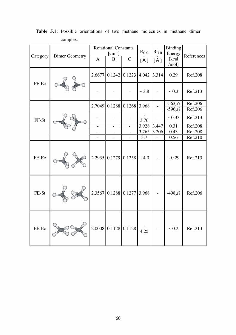
60

Table 5.1: Possible orientations of two methane molecules in methane dimer

complex.

Rotational Constants

[cm-1

] Category Dimer Geometry

A B C

RC-C

[o

A ]

RH-H

[o

A ]

Binding

Energy

[kcal

/mol]

References

2.6677 0.1242 0.1223 4.042 3.314 0.29 Ref.208

FF-Ec

- - - ~ 3.8 - ~ 0.3 Ref.213

-563µ? Ref.206 2.7049 0.1288 0.1268 3.968 -

-596µ? Ref.206

- - - ~

3.76 - ~ 0.33 Ref.213

- - - 3.928 3.447 0.31 Ref.208

- - - 3.765 3.206 0.43 Ref.208

FF-St

- - - 3.7 - 0.56 Ref.210

FE-Ec

2.2935 0.1279 0.1258 ~ 4.0 - ~ 0.29 Ref.213

FE-St

2.3567 0.1288 0.1277 3.968 - -498µ? Ref.206

EE-Ec

2.0008 0.1128 0,1128 ~

4.25 - ~ 0.2 Ref.213

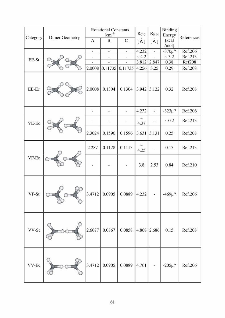
61

Rotational Constants

[cm-1

] Category Dimer Geometry

A B C

RC-C

[o

A ]

RH-H

[o

A ]

Binding

Energy

[kcal

/mol]

References

- - - 4.232 - -370µ? Ref.206

- - - ~ 4.2 - ~ 3.2 Ref.213

- - - 3.812 2.847 0.38 Ref208 EE-St

2.0008 0.11735 0,11735 4.256 3.25 0.29 Ref.208

EE-Ec

2.0008 0.1304 0.1304 3.942 3.122 0.32 Ref.208

- - - 4.232 - -323µ? Ref.206

- - - ~

4.37 - ~ 0.2 Ref.213

VE-Ec

2.3024 0.1596 0.1596 3.631 3.131 0.25 Ref.208

2.287 0.1128 0.1113 ~

4.25 - 0.15 Ref.213

VF-Ec

- - - 3.8 2.53 0.84 Ref.210

VF-St

3.4712 0.0905 0.0889 4.232 - -469µ? Ref.206

VV-St

2.6677 0.0867 0.0858 4.868 2.686 0.15 Ref.208

VV-Ec

3.4712 0.0905 0.0889 4.761 - -205µ? Ref.206

62

_____________________________________________________________________

CHAPTER 6

Theory of symmetric top molecules

_____________________________________________________________________

The different categories of molecules along with the most relevant theoretical

concepts to this work will be briefly covered in this chapter. More detailed discussion

of the following subjects can be found in (214-220).

6.1 Molecular Categories

In general, molecules can be classified based on the relative values of their three

principal moments of inertia labeled as IA, IB, and IC into four different groups as

follows:

– Linear molecules

These are mainly the molecules, in which all the atoms are aligned in a straight line,

so that the moment of inertia about the intermolecular axis is very small or zero.

Therefore, the moments of inertia are given as

IB

= IC and IA = 0 , e.g. HCN, HCl, OCS…

– Spherical top molecules

Molecules which have three identical moments of inertia

IA = I

B = I

C , e.g. SF6, SiH4, CH4 …

– Symmetric top molecules

Symmetric tops are the molecules which have two equal moments of inertia while the

third one is different. This group is divided into two classes:

63

• Oblate symmetric top molecules: (saucer or pancake shaped)

IA= I

B < I

C , e.g. BF3

• Prolate symmetric top molecules: (cigar shaped)

IB = I

C > I

A , e.g. CH3Cl…

– Asymmetric top molecules

These are the molecules to which the majority of substances belong and which have

three different moments of inertia given as

IA< I

B < I

C , e.g. H2O, CH2O, CH3OH

Where IA = Ixx, IB = Iyy, and IC = Izz in terms of the Cartesian coordinate system.

Upon the interaction with electromagnetic radiation, these molecules may experience

different types of motion: translational motion, rotational motion and vibrational

motion. Each atom in a molecule has three degrees of freedom, i.e. a molecule with N

atoms has 3N degrees of freedom. In translational motion (center of mass motion) the

entire molecule moves through space with a certain velocity and specific direction.

The velocity can be resolved into three different components in the Cartesian

coordinate system which means the total translational kinetic energy of the molecule

has also three components in the Cartesian coordinate system with the form

2222

2

1

2

1

2

1

2

1zyx mvmvmvmv ++= (6.1)

where v is the velocity and m is the mass of the molecule.

The molecule may rotate about some internal axis. The rotational motion can also be

resolved into three components in the x, y, z axes of the Cartesian coordinate system.

The rotational kinetic energy of the molecule consists then of three components in x,

y, z axis

64

222

2

1

2

1

2

1zzyyxxrot IIIE ωωω ++= (6.2)

where I is the moment of inertia and ω is the angular velocity. This equation indicates

that the molecule can have 3 or 2 different rotational degrees of freedom depending

on the type of the investigated molecule.

Finally, the molecule may also vibrate; in this case the number of vibrational degrees

of freedom (known also as vibrational modes) within the vibrating molecule is then

given by the remaining 3N-6 and 3N-5 degrees of freedom for nonlinear and linear

molecules respectively.

These motions can lead up to different types of molecular spectra depending on the

type of the molecule. For example, the motions that produce a net change in the dipole

moment of the molecule result in MW or IR spectra, whereas the motions that cause a

change in the polarizability of the molecule result in Raman spectra. The energies of

each category of molecules can be described by using Hamiltonians that should

include all the effective parameters of the molecular complex. The Hamiltonian can

then be solved by Schrödinger equation to determine the allowed energy levels of the

molecular complex.

In the present work, a high resolution infrared diode laser spectrometer is used to

investigate the spectra of the methane dimer complex (CH4)2 that can be classified as

a nearly symmetric top molecule. Therefore, it is expected to have a spectrum similar

to one of the limiting cases of symmetric top molecules. To achieve a better

understanding of the measured spectra, a short introduction on the theory of

symmetric top rotors will be given in this chapter. A more detailed discussion can be

found in (214-219).

6.2 Symmetric top molecules

The classical form of the rotational kinetic energy for a rigid symmetric top molecule

is

65

C

c

B

b

A

a

rotI

J

I

J

I

JE

222

222

++= (6.3)

where J is the angular momentum, and J2 for a three dimensional rotor is given by

2222

cba JJJJ ++= (6.4)

The starting Hamiltonian for the symmetric top rotor is the same as the one for the

general case of free rotating object in three dimensions written as

C

c

B

b

A

a

rotI

J

I

J

I

JH

2

ˆ

2

ˆ

2

ˆˆ

222

++= (6.5)

where (IA< I

B= I

C) and (I

A= I

B < I

C) are the two limiting cases of the prolate and

oblate symmetric tops.

The energy level pattern for the rotation of a rigid symmetric top, can be found by

solving the Schrödinger equation for Hamiltonian of the two limiting cases of the

prolate symmetric top (IA< I

B = I

C) and the oblate symmetric top (IA= IB < IC). This

consequently leads to the following two expressions that describe the possible energy

levels of the symmetric top rotors.

EJK

= BJ (J + 1) + (A – B) K2 for prolate top (6.6)

EJK

= BJ (J + 1) + (C – B) K2 for oblate top (6.7)

The A, B, and C are the rotational constants of the molecule which are defined in

terms of the energy units of wavenumbers (cm-1

) as

AcI

hA

28π= ,

BcI

hB

28π= ,

CcI

hC

28π= (6.8)

J is the total angular momentum quantum number, and K is the component of the

angular momentum on the principal rotational axis of the molecule which is the a-axis

for a prolate top or the c-axis for an oblate top.

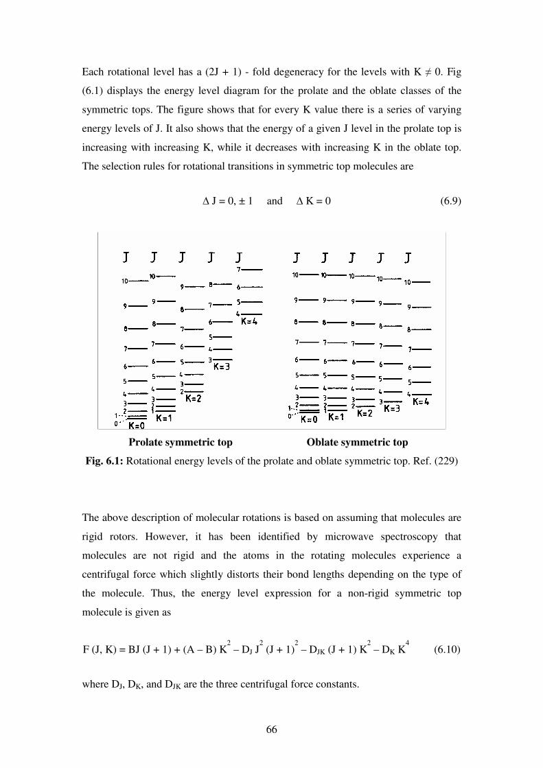
66

Each rotational level has a (2J + 1) - fold degeneracy for the levels with K ≠ 0. Fig

(6.1) displays the energy level diagram for the prolate and the oblate classes of the

symmetric tops. The figure shows that for every K value there is a series of varying

energy levels of J. It also shows that the energy of a given J level in the prolate top is

increasing with increasing K, while it decreases with increasing K in the oblate top.

The selection rules for rotational transitions in symmetric top molecules are

∆ J = 0, ± 1 and ∆ K = 0 (6.9)

Prolate symmetric top Oblate symmetric top

Fig. 6.1: Rotational energy levels of the prolate and oblate symmetric top. Ref. (229)

The above description of molecular rotations is based on assuming that molecules are

rigid rotors. However, it has been identified by microwave spectroscopy that

molecules are not rigid and the atoms in the rotating molecules experience a

centrifugal force which slightly distorts their bond lengths depending on the type of

the molecule. Thus, the energy level expression for a non-rigid symmetric top

molecule is given as

F (J, K) = BJ (J + 1) + (A – B) K2 – DJ J

2 (J + 1)

2 – DJK (J + 1) K

2 – DK K

4 (6.10)

where DJ, DK, and DJK are the three centrifugal force constants.

67

6.3 Asymmetric top molecules

Asymmetric top molecules comprise of the large majority of polyatomic molecules

which have no C3 axis of symmetry and with different moments of inertia given as

IA< IB < IC. The rotational spectra of this group of molecules are usually very

complex. The Schrödinger equation has no analytical solutions for the energy levels

of asymmetric tops analogous to that for the linear and the symmetric top molecules.

Therefore, the best approach is to consider the asymmetric tops as a case lying

between the prolate and the oblate limits of symmetric tops which leads to a relatively

good approximation of the energy levels of the asymmetric top molecule. This

indicates that the asymmetric rotors may include some symmetric top properties.

Considering the general case of a rigid rotor in three dimensions leads to the fact that

the angular momentum J can be represented as in equ. (6.4)

2222

cba JJJJ ++=

But the general case (IA ≠ IB ≠ IC) is practically the asymmetric top rotor, where the

quantum mechanical Hamiltonian operator of the asymmetric top is stated as in equ.

(6.5)

The Schrödinger equation of this Hamiltonian leads to the overall rotational energy of

the system along the three principal axes of inertia a, b, and c. These energy

eigenvalues are expressed in the form of

Ĥrot = A Ĵ

2

a + B Ĵ2

b + C Ĵ2

c (6.11)

where A, B, and C are rotational constants of the molecular system defined previously

in equ. (6.8) for symmetric top molecules.

AcI

hA

28π= ,

BcI

hB

28π= ,

CcI

hC

28π=

C

c

B

b

A

arot

I

J

I

J

I

JH

2

ˆ

2

ˆ

2

ˆˆ

222

++=

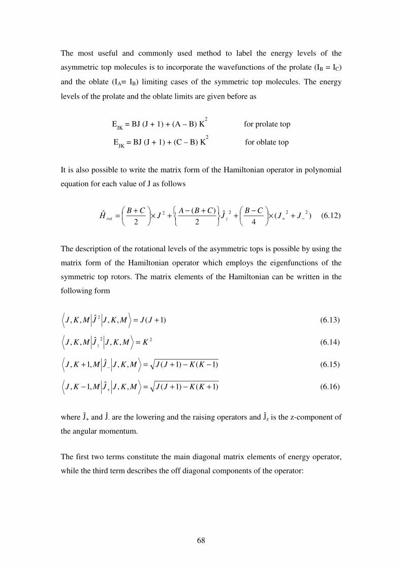
68

The most useful and commonly used method to label the energy levels of the

asymmetric top molecules is to incorporate the wavefunctions of the prolate (IB = IC)

and the oblate (IA= IB) limiting cases of the symmetric top molecules. The energy

levels of the prolate and the oblate limits are given before as

EJK

= BJ (J + 1) + (A – B) K2 for prolate top

EJK

= BJ (J + 1) + (C – B) K2 for oblate top

It is also possible to write the matrix form of the Hamiltonian operator in polynomial

equation for each value of J as follows

)(4

ˆ2

)(

2ˆ 2222

−+ +×

−+

+−

+×

+= JJ

CBJ

CBAJ

CBH zrot (6.12)

The description of the rotational levels of the asymmetric tops is possible by using the

matrix form of the Hamiltonian operator which employs the eigenfunctions of the

symmetric top rotors. The matrix elements of the Hamiltonian can be written in the

following form

)1(,,ˆ,, 2 += JJMKJJMKJ (6.13)

22,,ˆ,, KMKJJMKJ z = (6.14)

)1()1(,,ˆ,1, −−+=+ − KKJJMKJJMKJ (6.15)

)1()1(,,ˆ,1, +−+=− + KKJJMKJJMKJ (6.16)

where Ĵ+ and Ĵ- are the lowering and the raising operators and Ĵz is the z-component of

the angular momentum.

The first two terms constitute the main diagonal matrix elements of energy operator,

while the third term describes the off diagonal components of the operator:

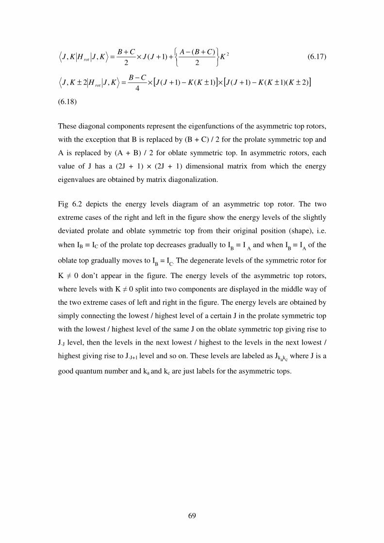
69

2

2

)()1(

2,, K

CBAJJ

CBKJHKJ rot

+−

++×+

= (6.17)

[ ] [ ])2)(1()1()1()1(4

,2, ±±−+×±−+×−

=± KKKJJKKJJCB

KJHKJ rot

(6.18)

These diagonal components represent the eigenfunctions of the asymmetric top rotors,

with the exception that B is replaced by (B + C) / 2 for the prolate symmetric top and

A is replaced by (A + B) / 2 for oblate symmetric top. In asymmetric rotors, each

value of J has a (2J + 1) × (2J + 1) dimensional matrix from which the energy

eigenvalues are obtained by matrix diagonalization.

Fig 6.2 depicts the energy levels diagram of an asymmetric top rotor. The two

extreme cases of the right and left in the figure show the energy levels of the slightly

deviated prolate and oblate symmetric top from their original position (shape), i.e.

when IB = IC of the prolate top decreases gradually to IB = I

A and when I

B = IA of the

oblate top gradually moves to IB = I

C. The degenerate levels of the symmetric rotor for

K ≠ 0 don’t appear in the figure. The energy levels of the asymmetric top rotors,

where levels with K ≠ 0 split into two components are displayed in the middle way of

the two extreme cases of left and right in the figure. The energy levels are obtained by

simply connecting the lowest / highest level of a certain J in the prolate symmetric top

with the lowest / highest level of the same J on the oblate symmetric top giving rise to

J-J level, then the levels in the next lowest / highest to the levels in the next lowest /

highest giving rise to J-J+1 level and so on. These levels are labeled as Jkakc where J is a

good quantum number and ka and kc are just labels for the asymmetric tops.

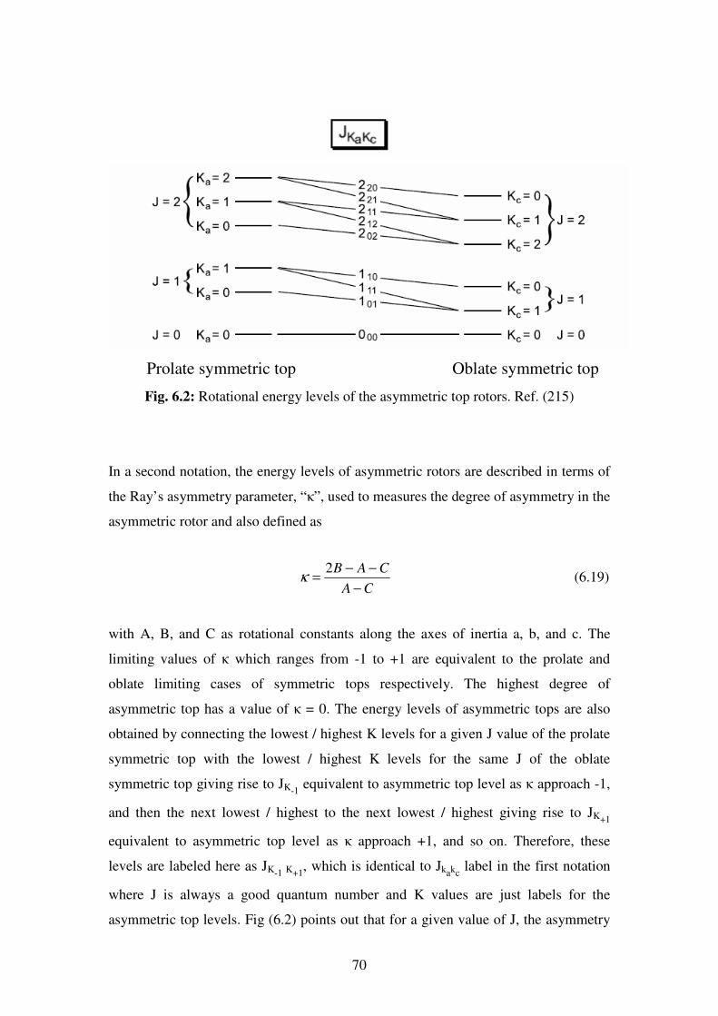
70

Prolate symmetric top Oblate symmetric top

Fig. 6.2: Rotational energy levels of the asymmetric top rotors. Ref. (215)

In a second notation, the energy levels of asymmetric rotors are described in terms of

the Ray’s asymmetry parameter, “κ”, used to measures the degree of asymmetry in the

asymmetric rotor and also defined as

CA

CAB

−

−−=

2κ (6.19)

with A, B, and C as rotational constants along the axes of inertia a, b, and c. The

limiting values of κ which ranges from -1 to +1 are equivalent to the prolate and

oblate limiting cases of symmetric tops respectively. The highest degree of

asymmetric top has a value of κ = 0. The energy levels of asymmetric tops are also

obtained by connecting the lowest / highest K levels for a given J value of the prolate

symmetric top with the lowest / highest K levels for the same J of the oblate

symmetric top giving rise to JK-1 equivalent to asymmetric top level as κ approach -1,

and then the next lowest / highest to the next lowest / highest giving rise to JK+1

equivalent to asymmetric top level as κ approach +1, and so on. Therefore, these

levels are labeled here as JK-1 K+1, which is identical to Jkakc

label in the first notation

where J is always a good quantum number and K values are just labels for the

asymmetric top levels. Fig (6.2) points out that for a given value of J, the asymmetry

71

splitting of K levels increase in energy as J increases for prolate top, while it

decreases in energy as K increase for oblate top.

6.4 Selection rules

The transitions in asymmetric top rotors are more complicated than the ones in linear

or symmetric top rotors. These transitions depend mainly on the symmetry of the

dipole moment components µa, µ

b and µ

c along their principal axis of inertia. Any

effective component of the dipole moments (µa, µ

b or µ

c ≠ 0) results in a set of certain

transitions in the molecule leading to different types of spectra. These spectra are

named as a-type, b-type and c-type spectra based on the individual dipole

components. The selection rules for these transitions are

a - Type: ∆ Ka = 0, (± 2, ± 4,…) and ∆ Kc = ± 1, (± 3, ± 5,…)

b – Type: ∆ Ka = ± 1, (± 3, ± 5,…) and ∆ Kc = ± 1, (± 3, ± 5,…)

c – Type: ∆ Ka = ± 1, (± 3, ± 5,…) and ∆ Kc = 0, (± 2, ± 4,…)

The selection rule for the total angular momentum J is ∆J = 0, ±1. An example for the

different types of transitions for the lowest Ka: 1 ← 0 transition is presented in Fig.

(6.3). The transitions for which the ∆ Ka and ∆ Kc values lie within the brackets are

only weakly allowed compared to the transitions corresponding to the values outside

the brackets.

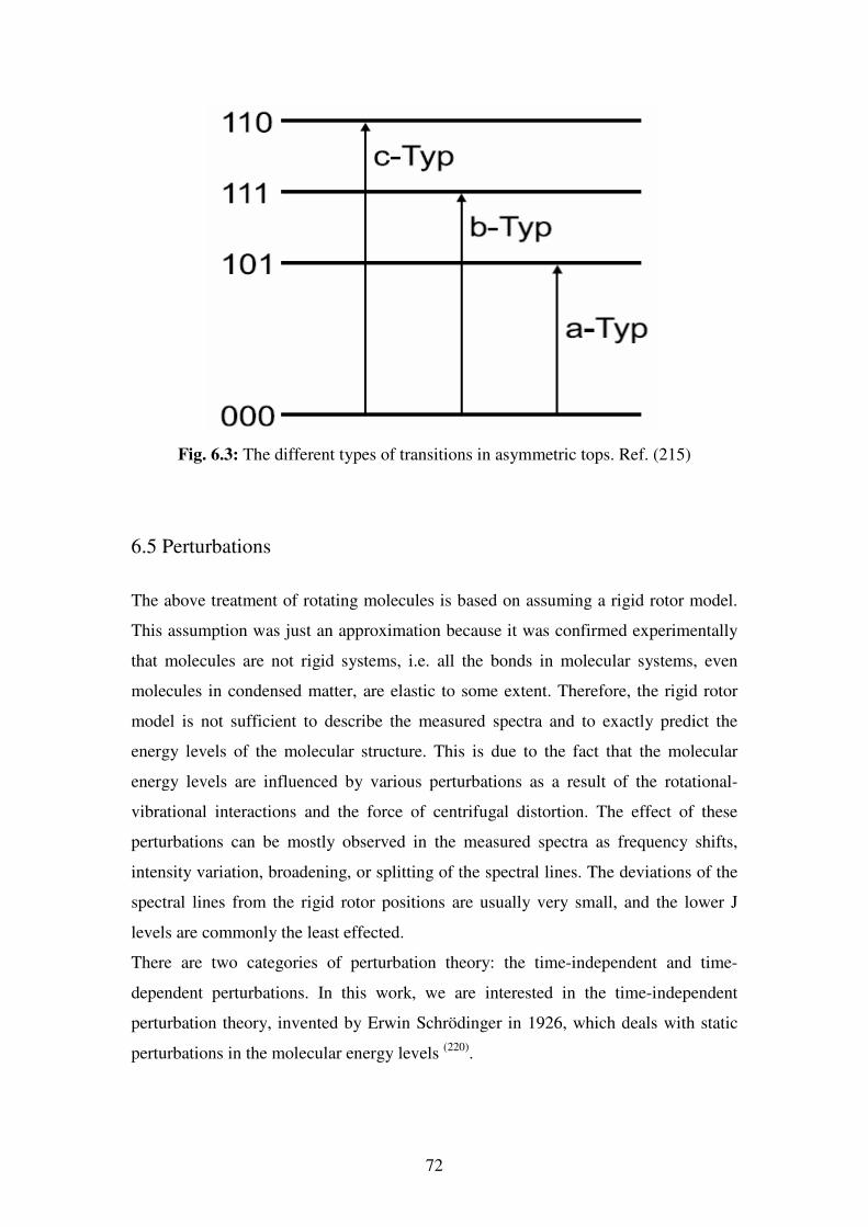
72

Fig. 6.3: The different types of transitions in asymmetric tops. Ref. (215)

6.5 Perturbations

The above treatment of rotating molecules is based on assuming a rigid rotor model.

This assumption was just an approximation because it was confirmed experimentally

that molecules are not rigid systems, i.e. all the bonds in molecular systems, even

molecules in condensed matter, are elastic to some extent. Therefore, the rigid rotor

model is not sufficient to describe the measured spectra and to exactly predict the

energy levels of the molecular structure. This is due to the fact that the molecular

energy levels are influenced by various perturbations as a result of the rotational-

vibrational interactions and the force of centrifugal distortion. The effect of these

perturbations can be mostly observed in the measured spectra as frequency shifts,

intensity variation, broadening, or splitting of the spectral lines. The deviations of the

spectral lines from the rigid rotor positions are usually very small, and the lower J

levels are commonly the least effected.

There are two categories of perturbation theory: the time-independent and time-

dependent perturbations. In this work, we are interested in the time-independent

perturbation theory, invented by Erwin Schrödinger in 1926, which deals with static

perturbations in the molecular energy levels (220)

.

73

To give a brief idea about the time-independent perturbation theory, we start by

considering an unperturbed Hamiltonian H0 which possesses no time dependence and

whose eigenfunctions ψn0

and eigenvalues En0

are known from the time-independent

Schrödinger equation

000

0 nnn EH ψψ = n = 0, 1, 2,… (6.20)

It is assumed here that En0 are discrete and non-degenerate. The 0 subscript indicates

that energies, wave functions and the Hamiltonian operators are of the unperturbed

system.

Now if we introduce a small perturbation to the system e.g. a weak physical

disturbance V like potential energy in an external field, then the resultant

modifications on ψn0 and En

0 can be determined by the perturbation theory. The

perturbed Hamiltonian is given by

H = H0 + λ V (6.21)

where λ is a dimensionless parameter that can take continuous values from 0

(perturbation off) to 1 (perturbation on). The eigenvalues and eigenstates of the

perturbed Hamiltonian are given by Schrödinger equation as

nnn EVH ψψλ =+ )( 0 (6.22)

If the perturbation is sufficiently weak, then the eigenvalues En and the eigenstates ψn

can be expressed in terms of a power series in λ:

En = En

0 + λ En

1 + λ

2 En

2 + ... (6.23)

...2210

+++= nnnn ψλψλψψ (6.24)

Substitution of the power series into the Schrödinger equation yields

( ) ( )......)(...)(20221010

0 +++++=+++ nnnnnnn EEEVH ψλψλλψλψλ (6.25)

74

It is evident that when λ = 0, all the values lead to the original values of the

unperturbed eigenvalues and eigenfunctions. As a result of small perturbation when λ

≠ 0, the energy levels and the eigenstates will not deviate much from their original

unperturbed values, therefore, the higher order terms will rapidly become smaller.

Consequently, the zeroth-order equation simply represents the Schrödinger equation

for the unperturbed system, while the first and the second order equations are

011001

0 nnnnnn EEVH ψψψψ +=+ (6.26)

02112012

0 nnnnnnnn EEEVH ψψψψψ ++=+ (6.27)

These can be used to derive the first order and the second order perturbations of the

system considering that H0, En0, ψn

0, and V are known values. The first order

perturbation theory is used to determine En1 and ψn

1.

Since ψn

1 in the first order

perturbation is not a known wave function, it has to be expressed as a series in terms

of complete set of orthogonal eigenfunctions

01

j

j

jn a ψψ ∑= (6.28)

ψj

0 is a complete orthogonal set of wave functions. Therefore, to determine the

perturbed eigenfunction ψn

1, the aj coefficients must be also determined. Substituting

this equation in the first order perturbation equation yields

010000

0 nnj

j

jnjj

j

j EaEVaH ψψψψ +=+ ∑∑ (6.29)

Taking a particular wave function ψm

0 out of the orthogonal set of wave functions ψj

0

and by using the orthogonality property of the ψj

0, where ‹ ψm

0 | ψj

0 › = 0 for m ≠ j

and ‹ ψm

0 | ψj

0 › = 1 for m = j, which can be expressed by Kronecker delta ‹ ψm

0 | ψj

0

› = δmj or ‹ ψm

0| ψj

0 › = δmn, one can get the first order correction term of the energy

for the perturbed system for m = n as follows

75

001

nnn VE ψψ= (6.30)

Therefore, the first order perturbation of the nth

state of a perturbed system is given by

000

nnnn VEE ψψλ+= (6.31)

For m ≠ n, the am coefficients are defined as

00

00

mn

nm

mEE

Va

−=

ψψ (6.32)

For m = n, the value of am =n can be calculated by using the normalization condition,

i.e. ‹ ψn

0 + λ ψn

1 | ψn

0 + λ ψn

1 › = 1 which gives the first order perturbation for the

wave function of the nth

state of the system as

0

00

00

0

m

nm mn

nm

nnEE

Vψ

ψψλψψ ×

−+= ∑

≠

(6.33)

The same analogy is used to obtain the second order perturbation for En2 and ψn

2,

where ψn2 is expressed in terms of a complete set of orthogonal wave functions of the

perturbed system as follows

02

j

j

jn b ψψ ∑= (6.34)

Now, substituting ψn

1and ψn

2 in the second order perturbation equation (6.27), leads to

021100000

nnj

j

nj

j

jnj

j j

jjjjj EEaEbaVEb ψψψψψ ++=+ ∑∑∑ ∑ (6.35)

Again, considering one specific wave function ψm0 of the complete orthogonal set of

the wave functions and then using the orthogonality function of ψj0 in terms of

Kronecker delta δmn leads to the second order correction term of the energy of the

perturbed system for m = n as

76

nnjn

j

jn aEVaE1002

−=∑ ψψ

= nnnnnjn

nj

j aEVaVa10000

−+∑≠

ψψψψ (6.36)

Using the equations of En1 and aj (am) in the first order perturbation, the second order

correction term of the energy of the perturbed system is then given by

∑≠ −

=nj jn

jn

nEE

VE

00

200

2ψψ

(6.37)

This equation indicates that the second order term increases drastically for closely

spaced energy levels, i.e. for small En0 – Ej

0.

For m ≠ n, the bm (bj) coefficients are expressed as

200

0000

0000

0000

)())(( jn

nmnn

nj jmjn

jmnj

mEE

VV

EEEE

VVb

−−

−−=∑

≠

ψψψψψψψψ (3.38)

For m = n, the value of bm = n can be found by using the normalization condition as

done in the first order which leads to

∑∑−

==200

200

2

)(2

1

2

1

jn

nj

j

jmEE

Vab

ψψ (6.39)

Therefore, the second order correction for the eigenfunction is given by

∑ ∑≠ ≠

−−

−−

−−=

nm nj

m

mn

nm

m

mn

nmnn

mnjn

jmnj

n

EE

V

EE

VV

EEEE

VV

0

200

200

0

200

0000

0000

0000

2

)(2

)())((

ψψψ

ψψψψψψψψψ

ψ (6.40)

77

6.6 Degeneracy

In the previous discussion, the first order correction of the wave function is obtained

based on the assumption that there is no degeneracy between the involved states n and

m, i.e. En

0 ≠ Em

0 in equation (6.33). If these states are degenerate in the original

unperturbed Hamiltonian, then the perturbation theory breaks down for these states

because the energy difference in the denominator (En

0 - Em

0) goes to zero and the

associated terms in the sum becomes infinite. However, this problem can be solved by

treating all the degenerate states as a linear combination of eigenstates of H0 with the

same eigenvalues. This is achieved by stating that n is M-fold degenerate with energy

En0 (220)

. The components of the unperturbed eigenfunctions are then denoted as ψni0

with i = 1, 2 …M, which share the same eigenvalues, i.e.

Edeg = En,1

0 = En,2

0 = En,3

0 = …= En,M

0 (6.41)

It is also possible to select these degenerate eigenstates to be orthogonal linear

combination of states which still have the same energy En0. Therefore, one can chose

a new set of M degenerate combinations as

∑=

=ΦM

j

njijnj b1

00 ψ (6.42)

The bij are the numerical coefficients, and the orthogonality condition leads to

ijnjni δ=ΦΦ00

(6.43)

The expansion for the jth

components of the degenerate set of eigenstates Φn,j0 and

then comparing the coefficients leads to

ijnjni EV δdeg

00=ΦΦ (6.44)

The selected degenerate states satisfy this equation and still remain eigenstates of H0.

This means that the perturbation does not mix the eigenstate members of the M

combination Φn,j0. Therefore, the first order wavefunction for any component of the

degenerate set is given by

78

0

00

00

1

i

i ni

nji

njEE

Vψ

ψψ ×

−

Φ−= ∑ (6.45)

Similarly, the second order energy can be expressed as

∑−

Φ−=

i ni

nji

njEE

VE

00

200

0ψ

(6.46)

The centrifugal distortion and Coriolis coupling are two examples of the time-

independent perturbation theory. These forces are present only when considering a

non-rigid rotor motion (rotating-vibrating molecule) with respect to a uniformly

rotating frame of reference. These forces result in a detectable effect on the rotational

energy levels which can be observed in the rotational spectra of the investigated

molecule. This makes the rigid rotor model a good basis for the treatment of these

interactions. However, for methane dimer, the experimental results show clear

evidence of coriolis interaction between the rovibronic levels. Therefore, the next

section will discuss the related aspects of coriolis interaction in non-rigid rotating

molecules

6.7 Coriolis Force

Coriolis effect is the apparent deviation of a freely moving object from its main

course as seen from a rotating frame of reference. This effect is referred to the

introduction of the Coriolis force which balances the equation of motion. The Coriolis

deflection is responsible for the counterclockwise rotation of tornados and hurricanes

in the northern hemisphere. This is because the earth's surface is rotating eastward at

greater speed near the equator than near the poles which makes the wind to shift to the

right in the northern hemisphere. Coriolis force is also very important in non-rigid

molecules. It is only effective in rotating and vibrating molecules where the motion

can be described in terms of a rigid rotor and the internal atomic vibrations about their

equilibrium positions. The atomic vibrations cause the atoms to move with respect to

the coordinate system of the rotating molecule. These atomic and molecular motions

produce a Coriolis effect which induces the atoms to move in a vertical direction to

the original oscillation leading to mixing between the rotational and vibrational

79

energy levels of the molecular system. The equation of motion describing the Coriolis

force is

( )ωξˆˆ2 ×= vmF (6.47)

where v is the velocity of the molecule relative to the molecule-fixed axis system (the

rotating system) and ω is the angular velocity of the molecule-fixed axis system (the

rotation rate). The formula indicates that the Coriolis force is perpendicular to both

the velocity of the moving molecular mass and the rotational axis. The physical

concepts of the Coriolis force as well as centrifugal force can be acquired by referring

to the classical representation of these forces presented in many reference books (214,

215, 218). A large number of experimental and theoretical work has been reported on

studying the different aspects of vibrational-rotational interactions in linear,

symmetric, and asymmetric top molecules. The detailed reviews of Nielsen (221)

and

Amat and Nielsen (222-224)

have a complete analysis of the non-rigid polyatomic

molecules where the Hamiltonian includes all possible interaction terms.

Under proper conditions, the Coriolis force can lead to considerable coupling between

rotational and vibrational motions of the molecular system. This in turn imposes

significant changes on the rigid rotor energy levels which may occur in either splitting

or shifting of the energy levels due to removal of degeneracy or to near degeneracy

respectively. For a given molecule, the vibrational-rotational interaction can be

described by the matrix element of the Coriolis coupling constant ζij(α)

which

represents the coupling of the rotation of two normal modes of vibration. This

indicates that the Coriolis coupling constants can be determined by the vibrational-

rotational constants α which are given by

αi = αi (harmonic)

+ αi (anharmonic)

+ αi (coriolis)

(6.48)

The Coriolis coupling has an observed effect on the spectra of linear, symmetric and

asymmetric top molecules with being more pronounced in symmetric top molecules

where first order effect is more common or possible. The vibrational-rotational bands

in the infrared region are those which experience pronounced deviations more often

due to Coriolis interactions. This effect on the rotational spectra of Van der Waal

weakly bound complexes will be discussed in this section taking the spectra of

80

methane argon (CH4-Ar) complex on the triply degenerate region ν4 as an example to

discuss our data of methane dimer (CH4)2 recorded in the same spectral region. The

rare gas-diatomic complexes (e.g. Ar-H2, and Ar-HF) have served as good models for

studying the dynamics and intermolecular potential in the weakly bound complexes

(225-228). The dynamics of these systems are very well understood and the most

accurate intermolecular potentials have been derived for these systems from which the

spectroscopic predictions appear to be in very good agreement with the latest

experimental data. The models of the rare gas-diatomic complexes can be extended to

study complexes of rare gas with other molecules such as rare gas-symmetrical,

spherical or asymmetric top complexes. The Hamiltonian for the rare gas-tetrahedral

molecular complexes can be formulated using the same method as for the rare gas-

diatomic complexes:

( )

),,(/ˆˆ

2

22

2

22

φθµ

RVHRR

jJH mon ++

∂∂−

−=h

(6.49)

where µ is the reduced mass of the complex, R is the distance between the center of

mass of the monomer molecule and the rare gas atom, Ĵ is the total angular

momentum of the complex, and j is the angular momentum of the monomer molecule.

The projections of ĵ on the molecules fixed axis z and on the body fixed axis Z are

designated as k and m respectively, but since the Ĵz is equivalent to ĵz, (Ĵz ≡ jz), then it

81

___________________________________________________________________________

CHAPTER 7

Measurements and Discussion

___________________________________________________________________________

In addition to presenting, discussing and analyzing the measured data of methane

dimer complex, this chapter will also cover a short summery on the symmetry of

tetrahedral molecules in order to have a better understanding of the energy levels of

such complexes. Comprehensive discussion of symmetry and the related topics in this

chapter can be found in references (214-219, 231).

7.1 Symmetry of Tetrahedral Molecules

In general, symmetry is a property of an object that is not influenced by the action of

certain movements or operations applied on the object such as rotation, reflection, and

translation, i.e. an object is said to be symmetrical if the object, when subjected to a

certain operation, appears exactly the same as before the operation applied with

respect to one or more of the geometrical symmetry elements, a point, a line, or a

plane. Symmetry has a fundamental contribution in understanding wide areas of

modern science especially in spectroscopy where it plays a central role in studying the

dynamical structure of a wide range of model systems. Symmetry has also been an

essential tool in studying theory and applications of dynamical systems and in orbital

theory calculations.

Molecules, like any other geometrical figure or object, may have one or more

symmetry elements. For example, a molecule may have an axis of symmetry around

which the molecule rotates leading to a configuration indistinguishable from the

original molecule before the rotation. The other symmetry elements, i.e. the center of

symmetry and the plane of symmetry, can also lead to the same result. On the other

hand, four different symmetry operations can also be applied to the molecule

(reflections σ, rotations Ĉn, rotation-reflections Ŝn and inversion ΐ). Each operation

transforms the molecule to an identical position of the original molecule before the

operation. Therefore, the use of symmetry in molecules is essential in understanding

82

the structures and properties of organic compounds and explaining many other

phenomena in chemistry and physics.

As a result of their natural high symmetry, tetrahedral molecules have been of special

interest to scientists in many research areas such as spectroscopy, crystal engineering,

polymers…etc. A detailed knowledge of these molecules can result in a better

understanding of molecular complexes involving tetrahedral molecules and how these

molecules behave and move within the molecular complexes. The symmetry

properties of tetrahedral molecules have been very useful in building up the

Hamiltonian of this group of molecules. The properties of highly symmetrical systems

don’t apply to the molecular complexes of tetrahedral molecules with other systems

(e.g. rare-gas tetrahedral complex), but most of these properties are preserved by the

tetrahedral molecule within the complex. This implies that the properties of the

complex must be invariant with respect to all possible internal rotations

(permutations) of the tetrahedral molecule within the complex which is equivalent

(isomorphic) to the point group T, where T is a subgroup of the full tetrahedral point

group Td that consists only of pure rotations of Td. The energy levels of the atom-

tetrahedral molecular complex can then be described in terms of having a good and

proper knowledge of the energy levels of the tetrahedral molecule in the complex.

Therefore, the following will be a short outline on the energy levels of the tetrahedral

molecules which is also extendable to other spherical top molecules that belong to Oh

and Ih point groups.

As classified among non-linear molecules, tetrahedral molecules may have 3N – 6

possible vibrational degrees of freedom. The most common and relatively simple

tetrahedral molecules of XY4 type have then (3N – 6) = 9 vibrational modes of

freedom. These modes, according to irreducible representations, are transformed to

A1, E, and two T2 of the Td point group. These species are designated conventionally

as ν1 (A1), ν2 (E), ν3 (T2), and ν4 (T2), where ν1 represent the symmetric stretching

mode, ν2 is the symmetric bending mode, ν3 is the asymmetric stretching mode, and ν4

represents the asymmetric bending mode. The ν3 and ν4 triply degenerate bands are the

only infrared active fundamental bands, i.e. bands that can produce infrared spectra as

a result of possessing electric dipole moment. The other two bands (ν1 and ν2) are low

intensity bands and can be induced through Coriolis coupling by the fundamental

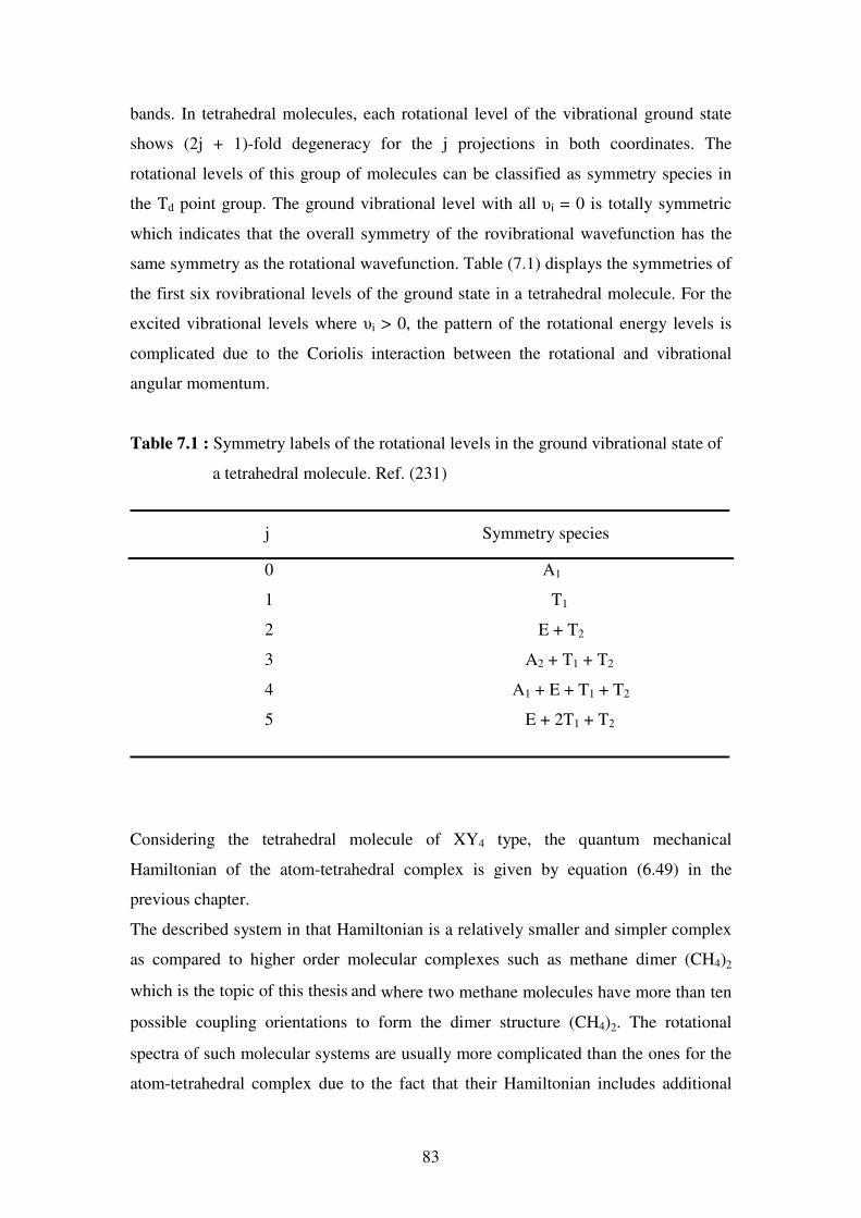
83

bands. In tetrahedral molecules, each rotational level of the vibrational ground state

shows (2j + 1)-fold degeneracy for the j projections in both coordinates. The

rotational levels of this group of molecules can be classified as symmetry species in

the Td point group. The ground vibrational level with all υi = 0 is totally symmetric

which indicates that the overall symmetry of the rovibrational wavefunction has the

same symmetry as the rotational wavefunction. Table (7.1) displays the symmetries of

the first six rovibrational levels of the ground state in a tetrahedral molecule. For the

excited vibrational levels where υi > 0, the pattern of the rotational energy levels is

complicated due to the Coriolis interaction between the rotational and vibrational

angular momentum.

Table 7.1 : Symmetry labels of the rotational levels in the ground vibrational state of

a tetrahedral molecule. Ref. (231)

_____________________________________________________________________

j Symmetry species

0 A1

1 T1

2 E + T2

3 A2 + T1 + T2

4 A1 + E + T1 + T2

5 E + 2T1 + T2

_____________________________________________________________________

Considering the tetrahedral molecule of XY4 type, the quantum mechanical

Hamiltonian of the atom-tetrahedral complex is given by equation (6.49) in the

previous chapter.

The described system in that Hamiltonian is a relatively smaller and simpler complex

as compared to higher order molecular complexes such as methane dimer (CH4)2

which is the topic of this thesis and where two methane molecules have more than ten

possible coupling orientations to form the dimer structure (CH4)2. The rotational

spectra of such molecular systems are usually more complicated than the ones for the

atom-tetrahedral complex due to the fact that their Hamiltonian includes additional

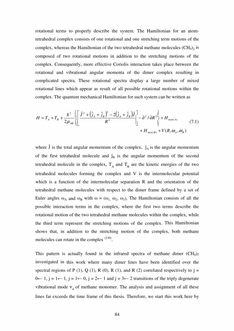
84

rotational terms to properly describe the system. The Hamiltonian for an atom-

tetrahedral complex consists of one rotational and one stretching term motions of the

complex, whereas the Hamiltonian of the two tetrahedral methane molecules (CH4)2 is

composed of two rotational motions in addition to the stretching motions of the

complex. Consequently, more effective Coriolis interaction takes place between the

rotational and vibrational angular momenta of the dimer complex resulting in

complicated spectra. These rotational spectra display a large number of mixed

rotational lines which appear as result of all possible rotational motions within the

complex. The quantum mechanical Hamiltonian for such system can be written as

( ) ( )

),,(

/ˆˆˆ2ˆˆˆ

2

)(

)(

22

2

222

BABmon

Amon

BABA

AB

BA

RVH

HRR

JjjjjJTTH

ωω

µ

++

+

∂∂−

+−++++=

h

(7.1)

where Ĵ is the total angular momentum of the complex, ĵA is the angular momentum

of the first tetrahedral molecule and ĵB is the angular momentum of the second

tetrahedral molecule in the complex, TA and T

B are the kinetic energies of the two

tetrahedral molecules forming the complex and V is the intermolecular potential

which is a function of the intermolecular separation R and the orientation of the

tetrahedral methane molecules with respect to the dimer frame defined by a set of

Euler angles ωA and ωB with ω = (ω1, ω2, ω3). The Hamiltonian consists of all the

possible interaction terms in the complex, where the first two terms describe the

rotational motion of the two tetrahedral methane molecules within the complex, while

the third term represent the stretching motions of the complex. This Hamiltonian

shows that, in addition to the stretching motion of the complex, both methane

molecules can rotate in the complex (230)

.

This pattern is actually found in the infrared spectra of methane dimer (CH4)2

investigated in this work where many dimer lines have been identified over the

spectral regions of P (1), Q (1), R (0), R (1), and R (2) correlated respectively to j =

0← 1, j = 1← 1, j = 1← 0, j = 2← 1 and j = 3← 2 transitions of the triply degenerate

vibrational mode ν4 of methane monomer. The analysis and assignment of all these

lines far exceeds the time frame of this thesis. Therefore, we start this work here by

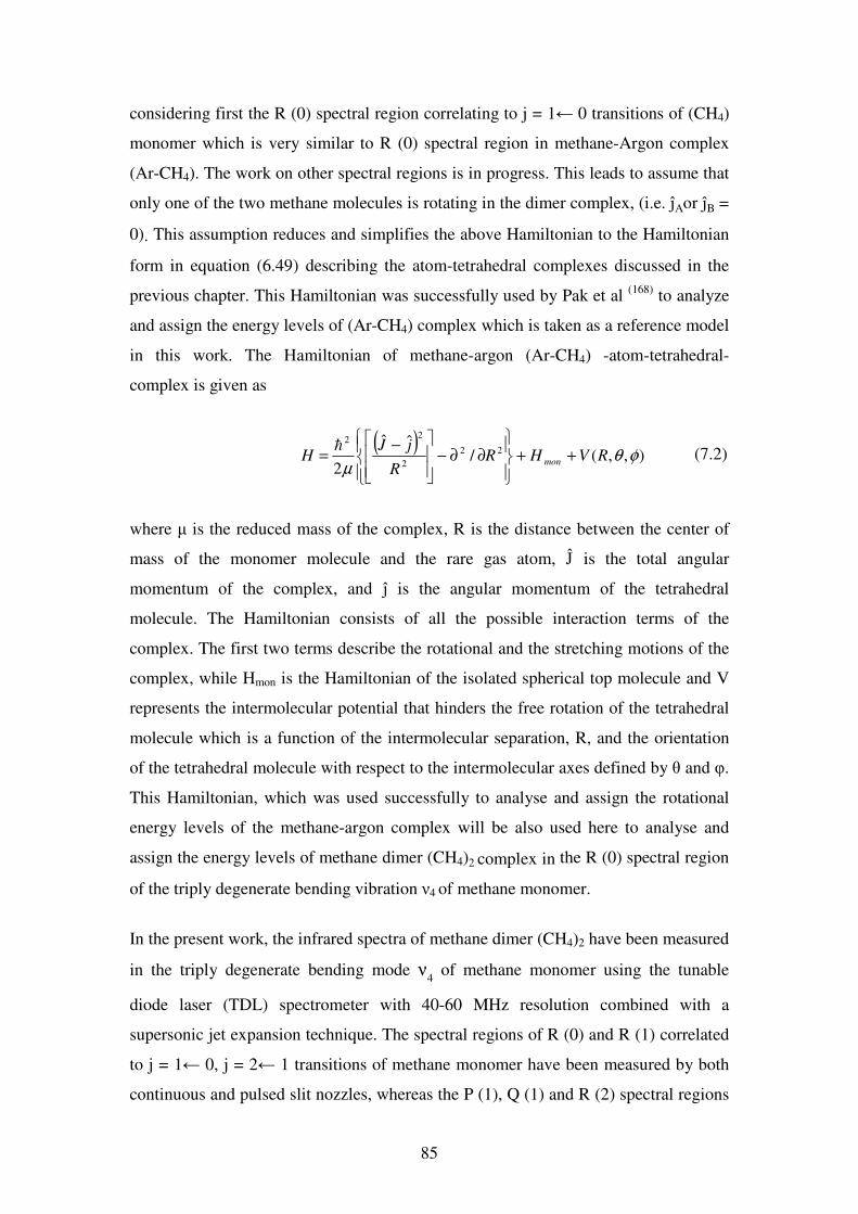
85

considering first the R (0) spectral region correlating to j = 1← 0 transitions of (CH4)

monomer which is very similar to R (0) spectral region in methane-Argon complex

(Ar-CH4). The work on other spectral regions is in progress. This leads to assume that

only one of the two methane molecules is rotating in the dimer complex, (i.e. ĵAor ĵB =

0). This assumption reduces and simplifies the above Hamiltonian to the Hamiltonian

form in equation (6.49) describing the atom-tetrahedral complexes discussed in the

previous chapter. This Hamiltonian was successfully used by Pak et al (168)

to analyze

and assign the energy levels of (Ar-CH4) complex which is taken as a reference model

in this work. The Hamiltonian of methane-argon (Ar-CH4) -atom-tetrahedral-

complex is given as

( )

),,(/ˆˆ

2

22

2

22

φθµ

RVHRR

jJH mon ++

∂∂−

−=h

(7.2)

where µ is the reduced mass of the complex, R is the distance between the center of

mass of the monomer molecule and the rare gas atom, Ĵ is the total angular

momentum of the complex, and ĵ is the angular momentum of the tetrahedral

molecule. The Hamiltonian consists of all the possible interaction terms of the

complex. The first two terms describe the rotational and the stretching motions of the

complex, while Hmon is the Hamiltonian of the isolated spherical top molecule and V

represents the intermolecular potential that hinders the free rotation of the tetrahedral

molecule which is a function of the intermolecular separation, R, and the orientation

of the tetrahedral molecule with respect to the intermolecular axes defined by θ and φ.

This Hamiltonian, which was used successfully to analyse and assign the rotational

energy levels of the methane-argon complex will be also used here to analyse and

assign the energy levels of methane dimer (CH4)2 complex in the R (0) spectral region

of the triply degenerate bending vibration ν4 of methane monomer.

In the present work, the infrared spectra of methane dimer (CH4)2 have been measured

in the triply degenerate bending mode ν4 of methane monomer using the tunable

diode laser (TDL) spectrometer with 40-60 MHz resolution combined with a

supersonic jet expansion technique. The spectral regions of R (0) and R (1) correlated

to j = 1← 0, j = 2← 1 transitions of methane monomer have been measured by both

continuous and pulsed slit nozzles, whereas the P (1), Q (1) and R (2) spectral regions

86

correlated to j = 0← 1, j = 1← 1 and j = 3← 2 transitions of methane monomer were

measured by continuous slit nozzle only. A large number of dimer lines have been

identified over the above regions. The dimer lines are more concentrated after the

band center of the ν4 vibrational mode of methane (1306.25 cm-1

) which covers the R

(0) and R (1) spectral regions. A lower number of dimer lines were identified in the P

(1), Q (1), and R (2) regions. As an example of the measured spectra from different

regions, fig (7.1-A) displays the spectra of methane in helium and in argon for part of

the R (0) spectral region, while fig. (7.1-B) represents the spectra for part of the R (1)

spectral region. The spectral gap between the two figures is mainly due to the mode

jumps in the radiation of the diode laser system. More than one laser diode laser have

been used to cover all spectral regions in this work which also can cause spectral gaps

in between the collectively measured spectra. The intensity of the dimer lines is not

absolute due to the laser power fluctuation across the radiation of a single mode and

between the different modes. Figure (7.2) is also another example showing two

spectra of the same spectral region measured with both continuous and pulsed slit

nozzles using methane in helium for the two scans.

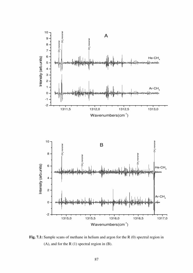
87

1311,5 1312,0 1312,5 1313,0

-2

-1

0

1

2

3

4

5

6

7

8

9

10

A

CH

4 m

onom

er

He-CH4

Ar-CH4

CH

4 m

onom

er

CH

4 m

onom

er

Inte

nsity (arb

.units)

Wavenumbers(cm-1)

1315,0 1315,5 1316,0 1316,5 1317,0

-2

0

2

4

6

8

10

B

CH

4 m

onom

er

CH

4 m

onom

er

CH

4 m

onom

er

He-CH4

Ar-CH4

CH

4 m

onom

er

Inte

nsity (arb

.units)

Wavenumbers(cm-1)

Fig. 7.1: Sample scans of methane in helium and argon for the R (0) spectral region in

(A), and for the R (1) spectral region in (B).

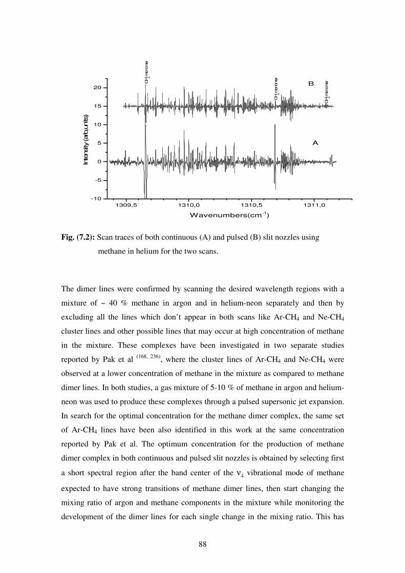
88

1309,5 1310,0 1310,5 1311,0

-10

-5

0

5

10

15

20B

ACH

4-m

onomer

CH

4-m

onomer

CH

4-m

onomer

Inte

nsity (arb

,units)

Wavenumbers(cm-1)

Fig. (7.2): Scan traces of both continuous (A) and pulsed (B) slit nozzles using

methane in helium for the two scans.

The dimer lines were confirmed by scanning the desired wavelength regions with a

mixture of ~ 40 % methane in argon and in helium-neon separately and then by

excluding all the lines which don’t appear in both scans like Ar-CH4 and Ne-CH4

cluster lines and other possible lines that may occur at high concentration of methane

in the mixture. These complexes have been investigated in two separate studies

reported by Pak et al (168, 236)

, where the cluster lines of Ar-CH4 and Ne-CH4 were

observed at a lower concentration of methane in the mixture as compared to methane

dimer lines. In both studies, a gas mixture of 5-10 % of methane in argon and helium-

neon was used to produce these complexes through a pulsed supersonic jet expansion.

In search for the optimal concentration for the methane dimer complex, the same set

of Ar-CH4 lines have been also identified in this work at the same concentration

reported by Pak et al. The optimum concentration for the production of methane

dimer complex in both continuous and pulsed slit nozzles is obtained by selecting first

a short spectral region after the band center of the ν4 vibrational mode of methane

expected to have strong transitions of methane dimer lines, then start changing the

mixing ratio of argon and methane components in the mixture while monitoring the

development of the dimer lines for each single change in the mixing ratio. This has

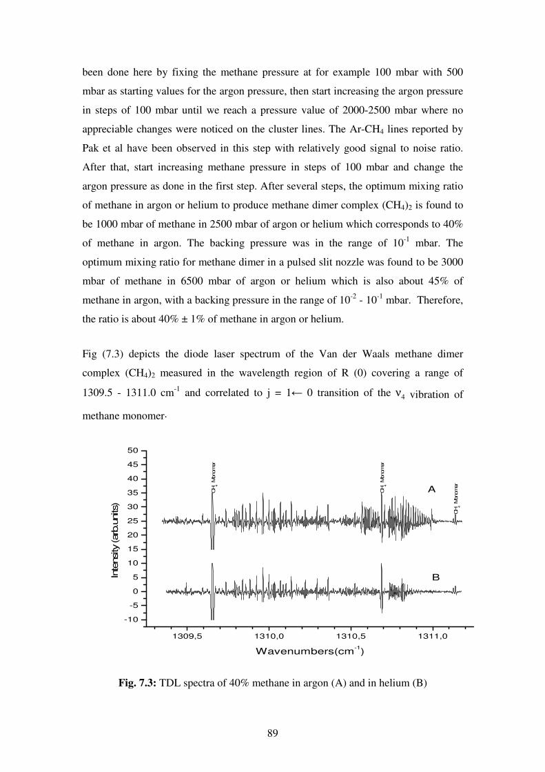
89

been done here by fixing the methane pressure at for example 100 mbar with 500

mbar as starting values for the argon pressure, then start increasing the argon pressure

in steps of 100 mbar until we reach a pressure value of 2000-2500 mbar where no

appreciable changes were noticed on the cluster lines. The Ar-CH4 lines reported by

Pak et al have been observed in this step with relatively good signal to noise ratio.

After that, start increasing methane pressure in steps of 100 mbar and change the

argon pressure as done in the first step. After several steps, the optimum mixing ratio

of methane in argon or helium to produce methane dimer complex (CH4)2 is found to

be 1000 mbar of methane in 2500 mbar of argon or helium which corresponds to 40%

of methane in argon. The backing pressure was in the range of 10-1

mbar. The

optimum mixing ratio for methane dimer in a pulsed slit nozzle was found to be 3000

mbar of methane in 6500 mbar of argon or helium which is also about 45% of

methane in argon, with a backing pressure in the range of 10-2

- 10-1

mbar. Therefore,

the ratio is about 40% ± 1% of methane in argon or helium.

Fig (7.3) depicts the diode laser spectrum of the Van der Waals methane dimer

complex (CH4)2 measured in the wavelength region of R (0) covering a range of

1309.5 - 1311.0 cm-1

and correlated to j = 1← 0 transition of the ν4 vibration of

methane monomer.

1309,5 1310,0 1310,5 1311,0

-10

-5

0

5

10

15

20

25

30

35

40

45

50

B

A

CH

4 M

onom

er

CH

4 M

onom

er

CH

4 M

onom

er

Inte

nsity (arb

.units)

Wavenumbers(cm-1)

Fig. 7.3: TDL spectra of 40% methane in argon (A) and in helium (B)

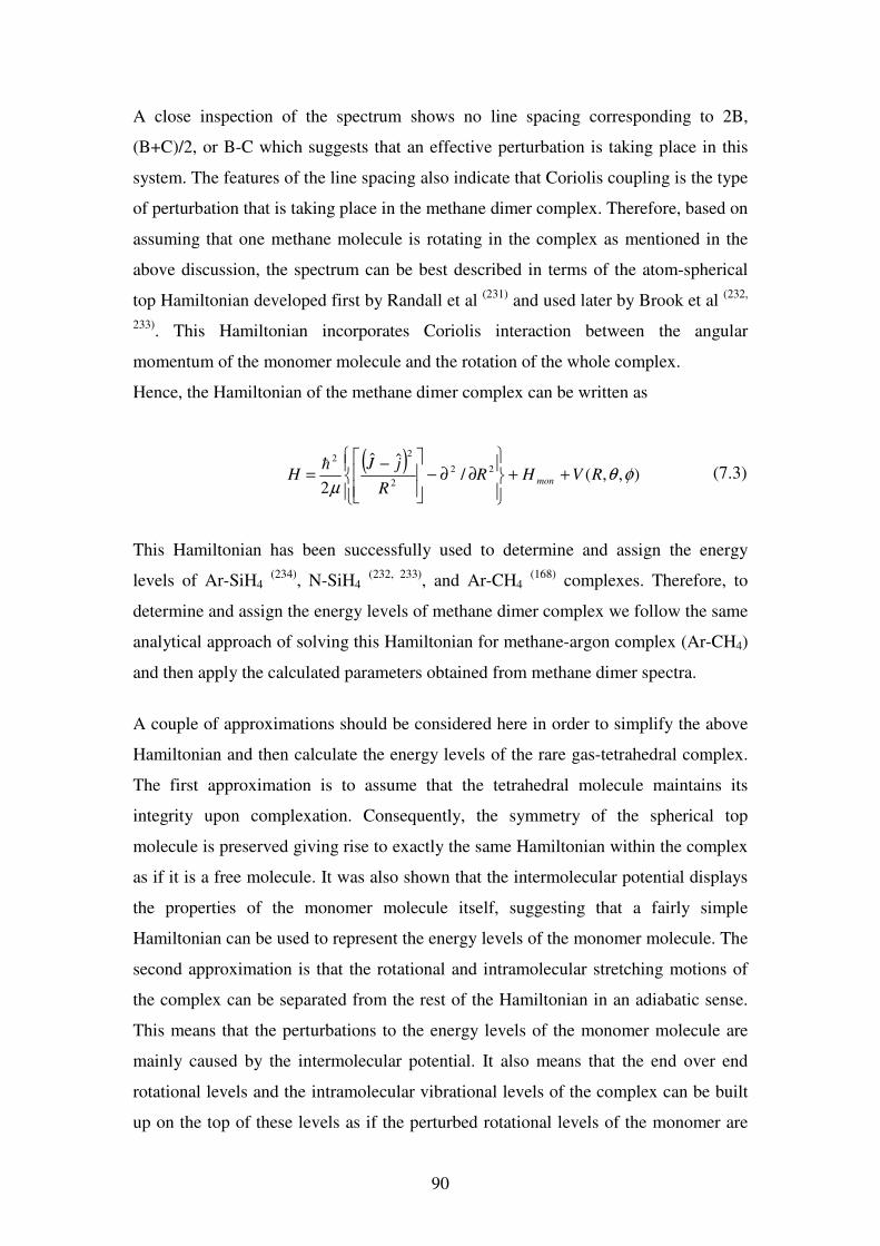
90

A close inspection of the spectrum shows no line spacing corresponding to 2B,

(B+C)/2, or B-C which suggests that an effective perturbation is taking place in this

system. The features of the line spacing also indicate that Coriolis coupling is the type

of perturbation that is taking place in the methane dimer complex. Therefore, based on

assuming that one methane molecule is rotating in the complex as mentioned in the

above discussion, the spectrum can be best described in terms of the atom-spherical

top Hamiltonian developed first by Randall et al (231)

and used later by Brook et al (232,

233). This Hamiltonian incorporates Coriolis interaction between the angular

momentum of the monomer molecule and the rotation of the whole complex.

Hence, the Hamiltonian of the methane dimer complex can be written as

( )

),,(/ˆˆ

2

22

2

22

φθµ

RVHRR

jJH mon ++

∂∂−

−=h

(7.3)

This Hamiltonian has been successfully used to determine and assign the energy

levels of Ar-SiH4 (234)

, N-SiH4 (232, 233)

, and Ar-CH4 (168)

complexes. Therefore, to

determine and assign the energy levels of methane dimer complex we follow the same

analytical approach of solving this Hamiltonian for methane-argon complex (Ar-CH4)

and then apply the calculated parameters obtained from methane dimer spectra.

A couple of approximations should be considered here in order to simplify the above

Hamiltonian and then calculate the energy levels of the rare gas-tetrahedral complex.

The first approximation is to assume that the tetrahedral molecule maintains its

integrity upon complexation. Consequently, the symmetry of the spherical top

molecule is preserved giving rise to exactly the same Hamiltonian within the complex

as if it is a free molecule. It was also shown that the intermolecular potential displays

the properties of the monomer molecule itself, suggesting that a fairly simple

Hamiltonian can be used to represent the energy levels of the monomer molecule. The

second approximation is that the rotational and intramolecular stretching motions of

the complex can be separated from the rest of the Hamiltonian in an adiabatic sense.

This means that the perturbations to the energy levels of the monomer molecule are

mainly caused by the intermolecular potential. It also means that the end over end

rotational levels and the intramolecular vibrational levels of the complex can be built

up on the top of these levels as if the perturbed rotational levels of the monomer are

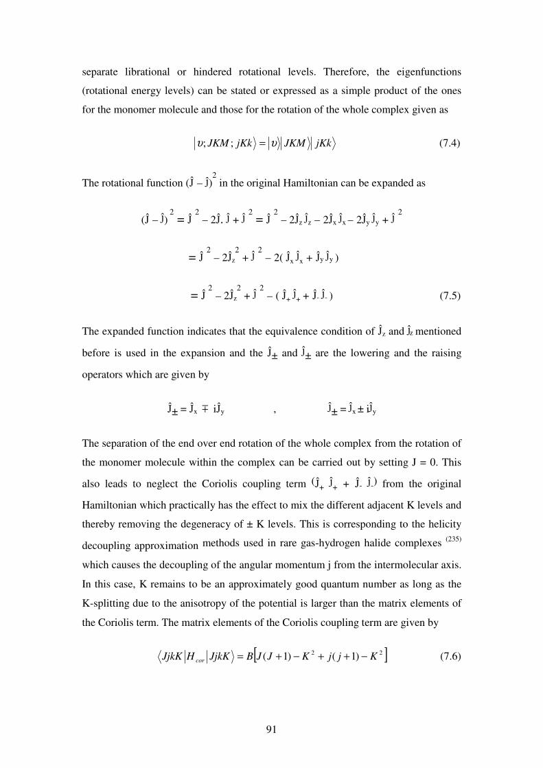
91

separate librational or hindered rotational levels. Therefore, the eigenfunctions

(rotational energy levels) can be stated or expressed as a simple product of the ones

for the monomer molecule and those for the rotation of the whole complex given as

jKkJKMjKkJKM υυ =;; (7.4)

The rotational function (Ĵ – ĵ)2 in the original Hamiltonian can be expanded as

(Ĵ – ĵ) 2 = Ĵ

2 – 2Ĵ. ĵ + ĵ

2 = Ĵ

2 – 2Ĵz ĵz – 2Ĵx ĵx – 2Ĵy ĵy + ĵ

2

= Ĵ 2 – 2Ĵz

2 + ĵ 2 – 2( Ĵx ĵx + Ĵy ĵy )

= Ĵ 2 – 2Ĵz

2 + ĵ 2 – ( Ĵ+ ĵ+ + Ĵ- ĵ- ) (7.5)

The expanded function indicates that the equivalence condition of Ĵz and ĵz mentioned

before is used in the expansion and the Ĵ± and ĵ± are the lowering and the raising

operators which are given by

Ĵ± = Ĵx m iĴy , ĵ± = ĵx ± iĵy

The separation of the end over end rotation of the whole complex from the rotation of

the monomer molecule within the complex can be carried out by setting J = 0. This

also leads to neglect the Coriolis coupling term (Ĵ+ ĵ+ + Ĵ- ĵ-) from the original

Hamiltonian which practically has the effect to mix the different adjacent K levels and

thereby removing the degeneracy of ± K levels. This is corresponding to the helicity

decoupling approximation methods used in rare gas-hydrogen halide complexes (235)

which causes the decoupling of the angular momentum j from the intermolecular axis.

In this case, K remains to be an approximately good quantum number as long as the

K-splitting due to the anisotropy of the potential is larger than the matrix elements of

the Coriolis term. The matrix elements of the Coriolis coupling term are given by

[ ]22 )1()1( KjjKJJBJjkKHJjkK cor −++−+= (7.6)

92

where Hcor represent the rotational term in the original Hamiltonian [(Ĵ – ĵ)2

× ħ2 / (2µ

R2 )], and B = ħ

2 / (2µ R

2 ) is the rotational constant of the complex.

The rotational energy levels of the complex can be expressed as a power series in [J (J

+ 1) – K2] rather than the usual power series in [J (J + 1)]. The obvious difference

between the two series is an energy shift of -B K2 in each energy level of the complex

leading to a shift in the band origin of the transition between two K states. On the

other hand, the effective rotational constant of the tetrahedral molecule is also affected

by the rotational constant of the whole complex B, (i.e. the monomer rotational

constant b becomes B + b). Therefore, this energy deviation of the level system

requires an explicit incorporation of the Coriolis coupling terms and to diagonalise a

proper 2×2 matrix for low j values. The main effect of Coriolis coupling terms is to

remove the degeneracy of the K = ± 1, ± 2, ± 3…levels for j = 1, 2, 3…etc. e.g. for j =

1 state, the K = 0 level couples to a symmetric combination of eigenfunctions with K

= 1 and K = -1, these states are

{ }112

11 −++=+ (7.7)

{ }112

11 −−+=− (7.8)

The K = 1 and K = -1 degeneracy of states is removed by the Coriolis interaction

because it only couples the K = 0 state with the symmetric combination | 1+ ›. The

Coriolis matrix element is then given by

)1()1(210 ** +×+=+ jjJJBH cor (7.9)

where j* is an empirical parameter equivalent to the effective value of j quantum

number.

This interaction has the influence to separate the | 0 › and | 1+ › levels apart from each

other while keeping the | 1- › level unaffected. Consequently, the rotational energy

levels associated with | 1+› state seem to have more energy separation than for K = 0

93

state which appear to be closer together, i.e. K = 0 is lower in energy than K = 1. The

resultant energy terms from the Hamiltonian can also be expressed in terms of the

splitting parameter (α) which also incorporates the effect of the intermolecular

potential and any vibrational terms, i.e. α measures the energy separation between K

levels. Therefore, by taking the energy of K = 0 and K = ± 1 as υE – α and υE + α

respectively, the rotational energy levels relative to the vibrational origins are given

by the eigenvalues of simple 2 × 2 matrix originated from the Coriolis matrix

elements in equ. (7.9)

+×+−

−+

=

=

)1()1(2

)1(

**

0

jjJJB

JJB

H

K α

++

+×+−

= α)1(

)1()1(2

1

**

JJB

jjJJB

K

(7.10)

where BK=0 and B

K=1 are the rotational constants for K = 0 and K = 1 levels

respectively, while B is taken as the effective mean value of these two constants. The

expression of the rotational energy levels is then given by diagonalizing the above 2 ×

2 matrix which results in the following eigenvalues

{ } 2/1**22222

10

)1()1(8)1()1(442

1

)1(2

++++∆++∆+±

+

++= ==

JJjjBJJBJBJ

JJBB

EE KK

J

αα

υ

(7.11)

where Eν is the vibrational energy and ∆B = B

K=1 – BK=0 which is highly correlated

with Coriolis terms leading to insufficient information about this factor. In this case, it

is adequate to constrain ∆B to zero in order to simplify the above equation to

)1()1(2)1( **22 +++±++= JJjjBJBJEEJ αυ (7.12)

In the vibrational excited state, the energy expression of the | 1- › level is given by

EJ = E

ν + α + B

K=1 J (J+1) (7.13)

For the states correlating to j = 0, the selection rules of the total angular momentum J

are

94

∆J = ± 1 for transitions to | 0 › and | 1+ › levels

∆J = 0 for transitions to | 1- › levels

The infrared spectroscopy of methane-argon complex (Ar-CH4) in the 7 micron region

investigated by Pak et al (168)

is a good example to get better understanding of the

above treatment for the atom-tetrahedral complex. The energy level diagram of

methane-argon is represented in Fig. (7.4), the left part of the figure shows the

rotational energy levels in the ground and excited vibrational states of methane, while

the rotational levels of the end over end rotation of the complex which are built on the

j, n levels of the methane part are located next to the left part and are defined by the

total angular momentum of the whole complex J. The right side of the figure displays

the splitting of the J levels in the upper vibrational state into its three components |1+›,

|1-›, and | 0›.

The recorded spectra were fitted using the above formulas for the ground and the

excited states where the strong transitions of R and P branches terminate in the lower |

0 › and upper |1+› Coriolis coupled levels respectively as shows in the figure.

However, it was difficult to precisely determine the rotational constant of these states

due to high correlation between these constants as a result of Coriolis coupling, i.e.

the dominated Coriolis terms cause mixing and splitting of the states of different K

producing the highly correlated rotational constants and dramatic change in the energy

of these levels. Then the transitions of the R and P branches can be expressed as

)1('')2/3()1(2)2)(1()( **

0 +−+×+×−+++= JJBJjjBJJBJJR υυ

( ){ } 2****

0 )1)(''()1()1(2'')1(2

1+−+++−+++−= JBBJjjBBBjjBυ (7.14)

)1('')2/1()1(2)1()( **

0 +−−×+×+−+= JJBJjjBJBJJP υυ

( ){ } 2****

0 )''()1(2'')1(2

1JBBJjjBBBjjB −++−+−+−= υ (7.15)

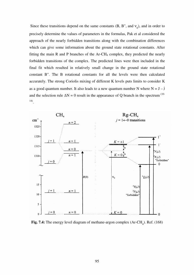
95

Since these transitions depend on the same constants (B, B", and ν0), and in order to

precisely determine the values of parameters in the formulas, Pak et al considered the

approach of the nearly forbidden transitions along with the combination differences

which can give some information about the ground state rotational constants. After

fitting the main R and P branches of the Ar-CH4 complex, they predicted the nearly

forbidden transitions of the complex. The predicted lines were then included in the

final fit which resulted in relatively small change in the ground state rotational

constant B". The B rotational constants for all the levels were then calculated

accurately. The strong Coriolis mixing of different K levels puts limits to consider K

as a good quantum number. It also leads to a new quantum number N where N = J – j

and the selection rule ∆N = 0 result in the appearance of Q branch in the spectrum (10-

14).

Fig. 7.4: The energy level diagram of methane-argon complex (Ar-CH4). Ref. (168)

96

7.2 Data Analysis

Fig (7.3) displays the spectrum of methane dimer recorded in the R (0) spectral region

correlating to j = 1← 0 transition of the triply degenerate mode ν4 of methane

monomer. The spectrum shows a strong and well resolved R branch starting at 1309.5

cm-1

, whereas the starting positions of the P and Q branch regions are estimated to be

around 1310.35 cm-1

and 1310.55 cm-1

respectively which exhibit very dense and

strong transition lines but with no obvious or resolved branch due to complex pattern

system for both regions. The intensity of the dimer lines is not absolute as the laser

power was changing across one single mode and between different modes. In the light

of the previous discussion, this spectrum can therefore be described and analyzed by

the Hamiltonian defined in equ. (7.3)

( )),,(/

ˆˆ

2

22

2

22

φθµ

RVHRR

jJH mon ++

∂∂−

−=h

This model incorporates Coriolis coupling between the hindered rotation of one

methane molecule and the rotation of the dimer complex. The perturbed rotational

energy levels of methane dimer are obtained by solving the Schrödinger equation of

this Hamiltonian. These states are represented in equations (7.12) and (7.13)

)1()1(2)1( **22 +++±++= JJjjBJBJEEJ αυ

EJ = E

ν + α + B

K=1 J (J+1)

These formulas are the basis of the fitting program developed and used in this work to

fit the transitions of methane dimer lines shown in Fig. (7.5) taking in account that the

strong transitions of the R and P branch terminate in the lower | 0 › and upper | 1+

›

Coriolis coupled levels respectively, while the transitions of the Q branch terminate in

the | 1- › level as shown in Fig. (7.4). These transitions satisfy the selection rules for

the states correlating to low j values (j = 0) where the total angular momentum ∆J = ±

1 for the | 0 › and | 1+ › states and ∆J = 0 for the | 1

- › states. Knowing and confirming

the position of R branch region from the fit leads us to estimate the positions of the P

97

and Q branch regions which are stated in the beginning of this section. This can be

used to calculate the lower and upper energy levels of the R, P, and Q branches using

equation (7.12). The result is a set of equations that can be solved by the fitting

program to give estimate values of the fitting parameters, i.e. the vibrational

frequency ( υE ), the Coriolis constant (C), and the splitting parameter (α). These

values are then used to predict the structure of methane dimer complex (CH4)2 and

compare it with the results of the ab initio theoretical predictions of the different

orientations of two methane molecules in a dimer complex list in chapter five.

Therefore, the lower and upper energy levels of R, P, and Q, branches of the dimer

complex are calculated as follows:

In R branch region, the energy of the lower level (j = 0, J = 0) is given as

00 =′′=JE

The energy of the upper level (J = 1) can be expressed as

22

1 22 CBEEJ +−+=′= αυ (7.16)

The line frequency is expressed as; ν = upper J – lower J

ν = E´J=1 – E´´

J=0

22 22 CBE +−+= αυ (7.17)

For the P branch, the energy of the lower level (J = 2) can be stated as

BE J 62 =′′= (7.18)

The energy of the upper level (J = 1) is given by

22

1 22 CBEEJ +++=′= αυ (7.19)

98

The line frequency can also be expressed as

ν = E´J=1 – E´´

J=2

22 24 CBE ++−= αυ (7.21)

For the Q branch region, the energy of the lower level (J = 1) is

BEJ 21 =′′= (7.22)

The energy of the upper level (J = 1) is given as

BEEJ 21 ++=′= αυ (7.23)

The line frequency is then give by

ν = E´J=1 – E´´

J=1

= Eν + α (7.24)

Solving these equations results in giving the estimated values of the unknown

parameters Eν, C, and α in the equations. The calculated values of these parameters,

taking B = 0.12 cm-1

, are given as:

Eν = 1310.05 cm-1

, C = 0.264721, α = 0.6985

These values are then used as starting input values in the fitting program in order to fit

the transition lines of methane dimer in Fig. (7.5). The outcome is a set of fitting

parameters shown in table (7.2), and the fitting results of the positions of the observed

dimer lines with respect to calculated positions are shown in table (7.3)

The absence of clear and well resolved P and Q branches in the spectrum led us to

start the fitting with R branch first and then follow the approach of line-by-line fitting.

This is mainly based on predicting the first line of the P or Q branch, the second line,

the third line and so on. Then make a fit of the predicted lines of each branch along

with the main fitted R branch in the spectrum and then do a final fit of the three

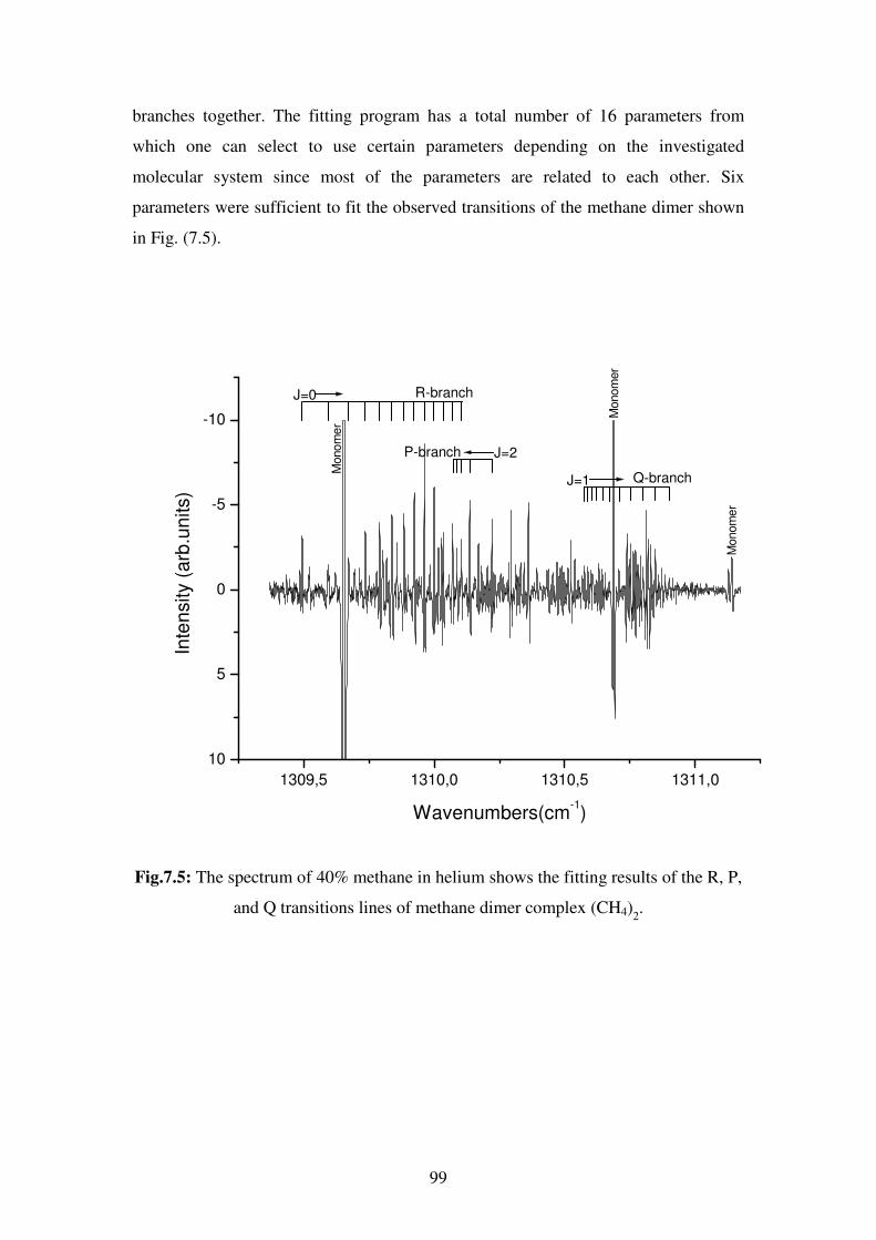
99

branches together. The fitting program has a total number of 16 parameters from

which one can select to use certain parameters depending on the investigated

molecular system since most of the parameters are related to each other. Six

parameters were sufficient to fit the observed transitions of the methane dimer shown

in Fig. (7.5).

1309,5 1310,0 1310,5 1311,0

10

5

0

-5

-10

Q-branch

P-branch

R-branch

J=1

J=2

J=0

Monom

er

Monom

er

Monom

er

Inte

nsity (

arb

.un

its)

Wavenumbers(cm-1)

Fig.7.5: The spectrum of 40% methane in helium shows the fitting results of the R, P,

and Q transitions lines of methane dimer complex (CH4)2.

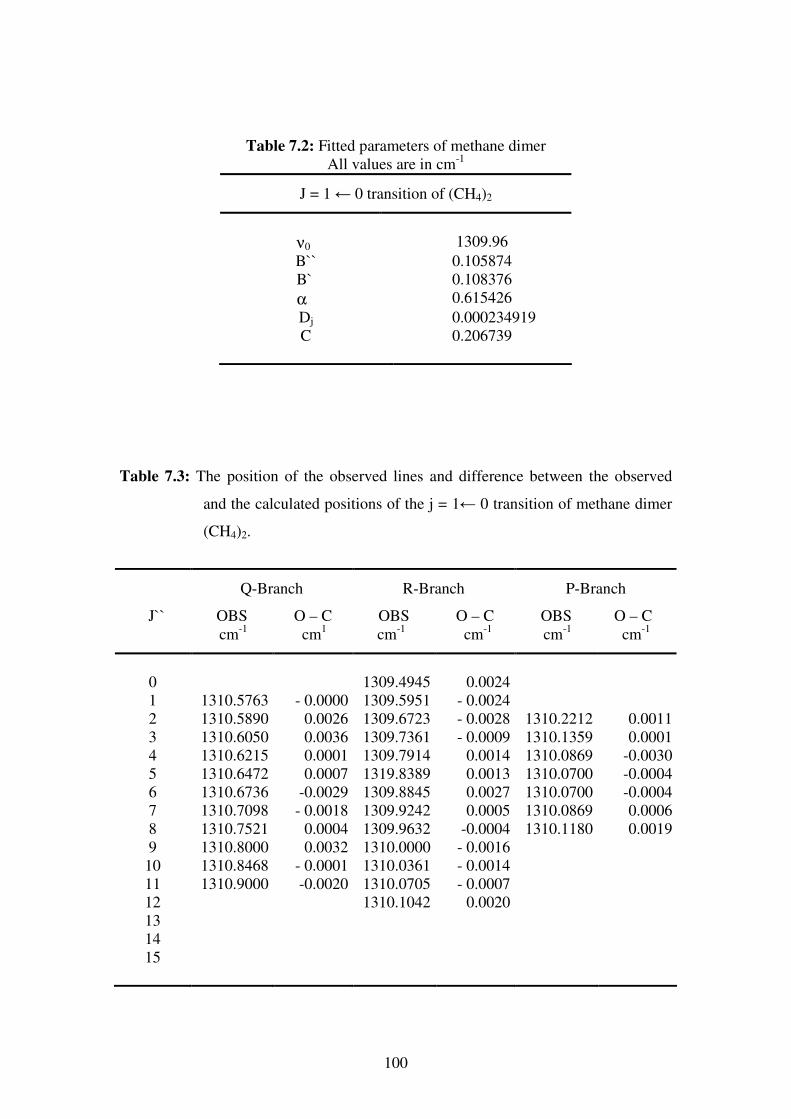
100

Table 7.2: Fitted parameters of methane dimer

All values are in cm-1

J = 1 ← 0 transition of (CH4)2

ν0 1309.96

B`` 0.105874

B` 0.108376

α 0.615426

Dj 0.000234919

C 0.206739

Table 7.3: The position of the observed lines and difference between the observed

and the calculated positions of the j = 1← 0 transition of methane dimer

(CH4)2.

Q-Branch R-Branch P-Branch

J`` OBS O – C OBS O – C OBS O – C

cm-1

cm1

cm-1

cm-1

cm-1

cm-1

0 1309.4945 0.0024

1 1310.5763 - 0.0000 1309.5951 - 0.0024

2 1310.5890 0.0026 1309.6723 - 0.0028 1310.2212 0.0011

3 1310.6050 0.0036 1309.7361 - 0.0009 1310.1359 0.0001

4 1310.6215 0.0001 1309.7914 0.0014 1310.0869 -0.0030

5 1310.6472 0.0007 1319.8389 0.0013 1310.0700 -0.0004

6 1310.6736 -0.0029 1309.8845 0.0027 1310.0700 -0.0004

7 1310.7098 - 0.0018 1309.9242 0.0005 1310.0869 0.0006

8 1310.7521 0.0004 1309.9632 -0.0004 1310.1180 0.0019

9 1310.8000 0.0032 1310.0000 - 0.0016

10 1310.8468 - 0.0001 1310.0361 - 0.0014

11 1310.9000 -0.0020 1310.0705 - 0.0007

12 1310.1042 0.0020

13

14

15

101

7.3 Discussion

Comparing the rotational constants of the fitted methane dimer in table (7.2) with the

calculated rotational constants of the theoretically predicted orientations of methane

dimer in table (5.1), we find that the value of B = 0.108376 cm-1

lies in between two

sets of orientations. The first set is EE-Ec and VF-Ec orientations which have a

rotational constant of 0.1128 cm-1

and the second set of orientations is VF-St and VV-

Ec which have a rotational constant of 0.905 cm-1

. These figures show that the

orientation of the two methane molecules in a dimer is not even close to the

equilibrium structure suggested by theoretical studies. The pattern of these values

indicates that the fitted B value of 0.108376 cm-1

is an average value of different

orientations of methane monomer in the complex which suggest the presence of large

amplitude motions. The fitted rotational constants can also be used to determine the

intermolecular distance R between the two methane molecules in the complex which

is calculated and found for j = 1 to be 4.46 Ao. The difference in the values of R in the

complex usually reflects the difference in the size of the complex.

Compared with other methane complexes such as Ar-CH4, Kr- CH4, and Ne-CH4, the

Coriolis constant C in methane dimer is higher than in Ar-CH4 and Kr- CH4, whereas

it is close to the value of Ne-CH4. This is due to the high value of rotational constant

B for (CH4)2 and Ne-CH4 and due to a high effective value of the rotational quantum

number for the monomer in the complex (j*). In methane dimer, this parameter has

been calculated for j = 1 and found to have a value of 0.9533 which is also higher than

the values of Ar-CH4 , Kr- CH4 and closer to the value of Ne-CH4 complex. This

indicates that the monomer in methane dimer is rotating more freely than in other

methane complexes. For example, the Coriolis constant in Ar-CH4 complex causes

stronger mixing between the K-levels in the system indicating a relatively stronger

intermolecular potential compared to the potential of methane dimer complex. This

can be inferred from the two values of (j*) for both complexes. The term α is the

splitting parameter between K = 0 and K = ± 1 levels before the Coriolis coupling

takes place. In a free rotor limit the splitting approach -2B`, i.e. α = -B`, this shows

that α +B` measures the effect of the anisotropy of the intermolecular potential (233)

.

Therefore, the smaller values of α + B` indicates a very weak anisotropic potential

102

like in which reflect the case Ne-CH4 and paraH2- CH4 complexes where the

monomer is close to free rotor limit.

7.4 Conclusion

The data analysis concludes that the geometry of the methane dimer complex is not

the equilibrium structure concluded by the ab initio theoretical studies. The analysis

also shows that the motion of the methane monomer in the dimer complex is close to

free rotor limit. Finally, the work on the other spectral regions of the triply degenerate

bending mode ν4 of methane monomer that have been measured in this work [P (1), Q

(1), R (1) and R (2)] is still in progress which in addition to analyzed data of the R (0)

spectral region in this thesis will help in the ongoing calculations of the intermolecular

potential of methane dimer complex.

103

BIBLIOGRAPHY

1- W. Kutzelingg: Einführung in die Theoretisch Chemie, Band 2, Kap. 15, Verlag

Chemie, (1978).

2- P.F. Bernath: Spectra of Atoms and Molecules, Oxford University Press (1995).

3- A.J. Stone: The Theory of Inermolecular Forces, Clarendon Press, Oxford (1996).

4- Chemical Reviews 6, 88, (1988).

5- Chemical Reviews 7, 94, (1994).

6- Chemical Reviews 11,100, (2000).

7- A. Sitlani and J. K. Barton, Biochemistry 33, 12100, (1994)

8- A. H. Krotz, T. P. S. L. Y. Kuo, and J. K. Barton, J. Am. Chem. Soc.115, 3877,

(1993).

9- B. Brutschy and P. Hobza, Chem.Rev. 100, (2000).

10- M. Scherer, Untersuchungen an schwach Molekül-Komplexen im Labor und im

Interstellaren Medium, Doktorarbeit, 2001.

11- M. Rigby, E.B. Smith, W.A. Wakeham, and G.C. Maitland, The Forces Between

Molecules, Oxford University Press, Oxford, (1986).

12- G.C. Maitland, M. Rigby, E.B. Smith, and W.A. Wakeham, Intermolecular

Forces: Their Origin and Determination, Oxford University Press, Oxford, (1981).

13- A. D. Bukingham, P.W. Fowler, J. Chem.Phys.79, 6426 (1983).

14- A. D. Bukingham, P.W. Fowler, A.J. Stone, Inter. Rev. Phys. Chem. 5, 107

(1986).

15- J.P. Toennies, Chem. Phys. Lett.20, 238, (1973).

16- J.M. Hutson, J. Chem. Phys.89, 4550, (1988).

17- J.M. Hutson, J. Chem. Phys.96, 6752, (1992).

18- R.C.Cohen, R.J. Saykally, J. Chem. Phys.98, 6007, (1993).

19- C.A. Schmuttenmaer, R.C.Cohen, R.J. Saykally, J. Chem. Phys.101, 146 (1994).

20- M.Quack, M. Suhm, . Chem. Phys.95, 28, (1991).

21- E.H.T. Olthof, A.van der Avoird, P.E.S. Wormer, Chem. Phys.101, 8430, (1994).

22- Hesse, R., Geoscience Canada, 14 (3) 165, (1986)

23- Sloan, E.D., Proc69th Ann Conv – Gas Process Assn., 69, 8, (1990)

24- G.F. Lindal, G.E. Wood, H.B. Hotz, D.N. Sweetnam, V.R. Eshleman, and G.L.

Tyler, Icarus 53, 348, (1983)

25- Sloan, E. D., Offshore Hydrate Engineering Handbook, ARCO, 1999.

104

26- Davy, H., Phil. Trans. Roy. Soc. London, 101, 1, (1811)

27- Faraday, M., Phil. Trans. Roy. Soc. London, 113, 160, (1823)

28- Hammerschmidt, E.G., Ind. Eng. Chem., 26, 851 (1934)

29- Hammerschmidt, E.G., Gas, 15 (5), 30, (1939)

30- Hammerschmidt, E.G., Oil Gas J, 29, (2) 61, (1940)

31- Frost, E.M. Jr., Deaton, W.M., Oil & Gas J, 45 (12), 170 (1946)

32- Deaton, W.M., Frost, E.M. Jr., Gas Hydrates and Their Relation to the Operation

of Natural-Gas Pipe Lines, 101 pp. U.S. Bureau of Mines Monograph 8, (1946)

33- Bond, D.C., Russell, N.B., Trans AIME, 179, 192, (1949)

34- Kobayashi, R., Vapour-Liquid Equilibrium in Binary Hydrocarbon-Water

systems, Ph.D Dissertation, U. Mich., (1951), University Microfilms No.3521,

Ann Arbor, MI

35- Woolfolk, R.M., Oil Gas J., 50(50), 124, (1952)

36- Makogon, Y.F., Gasov. Promst., 5, 14, (1965)

37- E.D. Sloan. Jr., Clathrate Hydrates of Natural Gases, 2nd

ed., revised and

expanded Marcel Dekker, Inc., New York, 1998

38- Von Stackelberg, M., Naturwiss, 36,327, (1949)

39- Von Stackelberg, M., Z. Electrochem., 58, 104, (1954a)

40- Von Stackelberg, M., Rec.Trav. Chim. Pays-Bas, 75, 902, (1956)

41- Von Stackelberg, M., Friibuss, H., Z. Electrochem., 58, 99, (1954b)

42- Von Stackelberg, M., Jahns, W., Z. Electrochem., 58, 162, (1954c)

43- Von Stackelberg, M., Meinhold, W., Z. Electrochem., 58, 40, (1954d)

44- Von Stackelberg, M., Muller, H.R, Z. Electrochem., 58, 25, (1954e)

45- Von Stackelberg, M., Muller, H.R, Naturwiss, 38, 456, (1951a)

46- Von Stackelberg, M., Muller, H.R, J. Chem. Phys., 19, 456, (1951b)

47- Claussen, W.F., J. Chem. Phys., 19, 259, 662, (1951a)

48- Claussen, W.F., J. Chem. Phys., 19, 1425, (1951b)

49- Pauling, L., Marsh, R.E., Proc. Nat.(U.S.A) Acad. Sci, 38, (1952)

50- Ripmeester, J.A., Tse, J.A., Ratcliffe, C.I., Powell, B.M., Nature, 325, 135, (1987)

51- Ripmeester, J.A., Ratcliffe, C.I., Tse, J.S., J. Chem. Soc Faraday Trans., 84, 3731,

(1988)

52- Ripmeester, J.A., Ratcliffe, C.I., McLaurin, G.E., The roll of Heavier

Hydrocarbons in Hydrates Formation, presented at AIChE meeting in Houston,

TX, (1991)

105

53- Mehta, A.P., Sloan, E.D., American Institute of Chemical Engineers (AIChE)

Journal, 42, 2036, (1996a)

54- Mehta, A.P., Sloan, E.D., American Institute of Chemical Engineers (AIChE)

Journal, 40, 312, (1996b)

55- Makogon, Y.F., Hydrates of Natural Gas, Moscow, Nedra, Izadatelstro, p. 208

(1974in Russian) Translated from Russian by W.J. Cieslesicz, PennWell Books,

Tulsa, Oklahoma p. 237 (1981 in English)

56- Edmonds, B., R. Moorwood, and R. Szczepanski , 1996, A practical Model for the

Effect of Salinity on Gas Hydrate Formation, SPE Paper 35569: SPE)

57- Kvenvolden, K.A., Collet, T.S., Lorenson, T.D., Biochemistry of Global Change,

487, (Oremland, R.S., ed), Chapman Hall, New York (1993a)

58- Kvenvolden, K.A., Ginsberg, G.D., Soloviev, V.A., Geo-Marine Lett., 13, 32,

(1993b)

59- Trofimuk, A.A., Cherskiy, N.V., Tsarev, V.P., Future Supply of Nature-made

Petroleum and Gas, (R.F. Meyer, ed), 919, Pergamon Press, New York, (1977)

60- Mclver, R.D., Long-term Energy Resources, (R.F. Meyer and J.C. Olsen, eds.),

Pitman, Boston, 1, 713, (1981)

61- Dobrynin, V.M., Korotajev, Yu.P., Plyushev, D.V., Long-term Energy Resources,

(R.G. Meyer, ed.), 727, Pitman, Boston, (1981)

62- Meyer, R.F., Long-term Energy Resources, (R.F. Meyer and J.C. Olsen, eds.), 49,

Pitman, Boston, (1981)

63- Makogon, Y.F., Natural Gs Hydrates: The State of Study in USSR and

Perspectives for its use, paper presented at the Third Chemical Congress of North

America, Toronto, Canada (1988b)

64- Kvenvolden, K.A., Chem. Geol., 71, 41, (1988a)

65- MacDonald, G.J., Climate Changes, 16, 247, (1990)

66- Gornitz, V., Fung, I., Global Biogeochemical Cycles, 8, 335, (1994)

67- Ginsberg, G.D., Soloviev, V.A., Proc.27th Ann Offshore Technology Conf. p.513,

Houston, OTC 7693, (1995)

68- R.S. Eng, J.F. Butler, K.J. Linden, Opt.Eng.19, 945, (1980)

69- K.J. Linden, A.W. Mantz, SPIE Proc.320, (1982)

70- S. König, Der Ar-CO van der Waal-komplex: Infrarotspektroskopie im

moleküljet, Dissertation, 1997.

71- G. Gimmler, Aufbau und Erprobung einer neuen Computersteuerung für ein

106

Diodenlaser-Spektrometer, Diplomarbeit, 1997.

72- E. Kapon, A. Katzir, IEEE J. Quant. Electronic. 21, 1947, 1985

73- K.J. Linden, IEEE J. Quant. Electronic. 21, 391, 1985

74- M. Petri, M. Schaefer, W. Urban, to be published

75- I. Scheela, Hochauflösene Infrarot-Spektroskopie an schwach gebundenen Van-

der-Waal-systemen, Doktorarbeit, 2001.

76- M. Schaefer, PhD thesis, Bonn 1995.

77- R. Lehing, Aufbau einer Herriott-Vielfachreflexionszelle für einDioden-

laserspektrometer und Spektroskpie des Ar-CO, Diplomarbeit, 2000.

78- J.A. Silver, Frequency-modulation for trace species detection: theory and

comparison among experimental methods, Appl. Opt. 31, 707, (1992)

79- D.S. Bomse, A. C. Stanton and J.A. Silver, Frequency modulation and wavelength

modulation spectroscopies: comparison of experimental methods using lead-salt

diode lasers, Appl. Opt. 31, 718, (1992)

80- A. Kantrowitz and J.Grey, Rev. Sci. Instru. 22, 328, (1951)

81- W. Gerlach and O. Stern, Z. Phys. 8, 110, (1921)

82- W. Gerlach and O. Stern, Z. Phys. 9, 349, 353, (1921)

83- O. Stern, Z. Phys., 7, 249, (1921)

84- R. N. Zare and P. J. Dagdigian, Science 185, 739, (1974).

85- G. Scoles, Atomic and Molecular Beam Methods, Volume 2 (Oxford University

Press, Oxford, 1992).

86- G. Scoles, Atomic and Molecular Beam Methods, Volume 1 (Oxford University

Press, Oxford, 1988).

87- J. Anderson, Molecular Beams and Low Density Gas Dynamics ~Marcel Dekker,

New York, pp. 1–91, (1974)

88- W. Demtröder, Laserspektroskpie, Springer, Berlin, 1991

89- Molecular Beam and Low Density Gasdynamics, edited by P.P. Wegener (Marcel

Deker, New York 1974)

90- R.B. Bernstein, Chemical Dynamics via Molecular Beam and Laser Techniques

(Oxford University, New York 1982)

91- M. Havenith, Infrared spectroscopy as a tool for understanding of intermolecular

forces, Habilitation, 1997

92- I. Scheela, Untersuchungen zum Verhalten der Schlitzdüsenexpansion am

Diodenlaserspektrometer und Spektroskopie des Ar-CO, Diplomarbeit, 1997

107

93- U. Merker, Aufbau und Optimierung eins CO-Seitenbandlaser für die

Spektroskopie am Molekularstrahl, Diplomarbeit, 1994

94- G. Scoles, Atomic and molecular beam methods, Oxford University Press,

Oxf.1988

95- O.F. Hagena, Nucleation and growth of clusters in expanding nozzle flows,

Surface Science, 106, 101 (1981)

96- Fluendy, M.A.D and Lawley, K.P. Chemical applications of molecular beam

scattering (Chapman and Hall, London), (1973a)

97- Olsen, R.M. Essentials of engineering fluid mechanics (Intext, New York),

(1973)

98- Levy, D. H. Ann. Rev. Phy. Chem. 31, 197, (1980)

99- N. Abuaf, J. B. Anderson, R. P. Andres, J. B. Fenn, and D. G.H. Marsden,

Science,155, 997, (1967).

100- W.R. Gentry, Low-energy pulsed beam sources, 54 in ref. 94, (1988)

101- C.M. Lovejoy, Ph.D, University of Colorado, (1990).

102- C.M. Lovejoy and D. J. Nesbitt, Rev. Sci. Instrum. 58, 807, (1987)

103- J. Nesbitt, Ann. Rev. Phys. Chem. 45, 367, (1994)

104- R.J. Sakally and G.A. Blake, Science, 259, 1570 (1993)

105- A. Amirav, U. Even and J. Jortner, Absorption spectroscopy of ultra-cold large

molecules in planar supersonic expansions, Chem. Phys. Lett. 83, 1, (1981)

106- C.M. Lovejoy and D.J. Nesbitt, Slit pulsed valve for generation of long-path-

length supersonic expansions, Rev. Sci. Instru. 58, 807, (1987)

107- S.W. Sharpe, R. Sheeks, C. Wittig, and R.A. Beaudet, Infrared absorption

spectroscopy of CO2-Ar complexes, Chem. Phys. Lett. 151, 267, (1988)

108- A. De Piante, E.J. Campbell and S.J. Buelow, Pulsed molecular-beam diode-

laser spectrometry using rapid scanning techniques, Rev. Sci. Instru. 60, 858,

(1989)

109- K. Liu, R.S. Fellers, M.R. Viant, R.P. McLaughlin, M.G. Brown and R.J.

Saykally, A long path length pulsed slit valve appropriate for high temperature

operation: Infrared spectroscopy of jet-cooled large water clusters and

nucleotide bases, Rev. Sci. Instru. 67, 410, (1996)

110- T.A. Hu, E.L. Chappell and S.W. Sharpe, Infrared diode laser spectroscopy of

the Ar-N2O complex: Observation of the intermolecular bending mode in

combination with the highest frequency intramolecular stretching mode, J.

108

Chem. Phys. 98, 6162, (1993)

111- K. Veeken and J. Reuss, Infrared line narrowing and cluster absorption in planar

jet, Appl. Phys. B 38, (1985)

112- G.A. Bethardy and D.S. Perry, Rate and mechanisim of intramolecular

vibrational redistribution in the ν16 asymmetric methyl strech band of 1-butyne,

J. Chem. Phys. 98, 6651, (1993)

113- M.D. Brookes and R.W. McKellar, The mystery of the CO-dimer: assignments

from variable-temperture jet-cooled infrared spectra, Chem. Phys. Lett. 287,

365, (1998)

114- M.D. Brookes and R.W. McKellar, infrared spectrum of the water-carbon

monoxide in the CO stretching region, J. Chem. Phys. 109, 5823, (1998)

115- M.D. Brookes and R.W. McKellar, Infrared spectrum and energy levels of the

CO-dimer: Evidence for two almost isoenergetic isomers, J. Chem. Phys. 111,

7321(1999)

116- C. Xia, A.R.W. McKellar and Y. Xu, Infrared spectrum of CO-N2 Van der

Waals complex: Assignments for the CO-paraN2 and observation of a bending

state for CO-orthoN2, J. Chem. Phys. 113, 525, (2000)

117- I. Pak, M. Hepp, D.A. Roth, and G. Winnewisser, A combined absorption-

wavelength modulation technique for diode laser spectroscopy of Van der Waal

complexes in a pulsed planar jet, Rev. Sci. Instru. 68, 1668, (1997)

118- S.W. Sharpe, Y.P. Zeng, C. Wittig, and R.A. Beaudet, Infrared absorption

spectroscopy of CO2-Hx complexes using the CO2 asymmetric stretch

chromophore: CO2-HF(DF) and CO2-HCl(DCl) linear and CO2-HBr bent

equilibrium geometries, J. Chem. Phys. 92, no. 2,943, (1990)

119- S.W. Sharpe, D. Reifschneider, C. Wittig, and R.A. Beaudet, Infrared absorption

spectroscopy of CO2-Ar complexes in the 2376 cm-1

combination band region:

The intermolecular bend, J. Chem. Phys. 94, 1, 233, (1991)

120- C. Dutton, A. Sazonov and R.A. Beaudet, High resolution ro-vibrational

absorption spectrum of CO2-N2O, J. Chem. Phys. 100, 17772, (1996)

121- H.B. Quian, W.A. Herrebout and B.J. Howard, Infrared diode laser jet

spectroscopy of the Van der Waals (N2O)2, Molec.Phys. 91, 689, (1997)

122- W.A. Herrebout, H.B. Quian, H. Yamagushi and B.J. Howard, High-resolution

infrared diode laser spectroscopy of Ne- N2O, Kr- N2O and Xe- N2O, J. Molec.

109

Spectrosc. 189, 235, (1998)

123- I. Pak, M. Hepp, R. Phillip, R. Schieder, and G. Winnewisser, Double

modulation technique in pulsed jet experiments with tunable diode lasers, Z.

Naturforsch. 49a, 913, (1994)

124- H.B. Quian, and B.J. Howard, High-resolution infrared spectroscopy and

structure of CO-N2O, J. Molec. Spectrosc. 184, 156, (1997)

125- G. Gimmler, Hochauflösene Infrarot-Spektroskopie an den Van-der-Waals-

Komplexen N2O-H2O und N2O-Ar, Doktorarbeit, 2001.

126- A.S. Pine, W.J. Lafferrty, J. Chem. Phys. 78, 2154, (1983)

127- R.E. Miller, J. Phys. Chem. 90, 331,(1986)

128- D.J. Nesbitt, Chem. Rev. 88, 843, (1988)

129- K.L. Busarow, G.A. Blake, K.B. Laughlin, R.C. Cohen, Y.T. Lee, R.J. Saykally,

Chem. Phys. Lett. 141, 289, (1987)

130- D.J. Prichard, R.N. Nandi, J.S. Muenter, J. Chem. Phys. 89, 115, (1988)

131- A.S. Pine, G.T. Fraser, J. Chem. Phys. 89, 100, (1988)

132- A.B. Rakshit, C.S. Roy, and A.K. Barua, J. Chem. Phys. 59, 3633, (1973)

133- J. Kestin, and S.T. Ro, Ber. Bunsenges. Phys. Chem.78, 20, (1974)

134- J. Kestin, and S.T. Ro, Ber. Bunsenges. Phys. Chem.80, 619, (1976)

135- T. Jacobs, L. Peters, and J. Vermant, Buil.Soc. Chem. Belges. 79, 337, (1970)

136- R.T. Trengove, H.L Robjohns, and P.J. Duntop, Ber. Bunsenges. Phys. Chem.86,

951, (1982)

137- P.J. Duntop, and C.M. Bignell, Physica A 145, 584, (1987)

138- G. Thomaes, R. van Steenvinkel, and W. Stone, Mol. Phys. 5, 301, (1962)

139- J. Brewer, AFOSR report No. MRL-2915-C (1967)

140- M.A. Byrne, M.R. Jones, and L.A.K. Staveley, Trans. Faraday Soc. 64, 1747,

(1968)

141- R.N. Lichtenthaler, and K. Schäfer, Ber. Bunsenges. Phys. Chem. 73, 42, (1969)

142- K. Stern, R.N. Lichtenthaler, B. Schramm, and K. Schäfer, Ber. Bunsenges.

Phys. Chem. 78, 287, (1971)

143- R. Hahn, K. Schäfer, and B. Schramm, Ber. Bunsenges. Phys. Chem.78, 287,

(1974)144- J. Bellm, W. Reineke, K. Schäfer, and B. Schramm, Ber. Bunsenges.

Phys. Chem.78, 282, (1974)

145- M.L. Martin, R.T. Trengove, K.R. Harris, and P.J. Duntop, Aust. J. Chem. 35,

1525, (1982)

110

146- G.A. Stevens and A.E. de Vries, Physica A 39, 346, (1968)

147- S. Acharyya and A.K. Barua, J. Phys. Soc. Jpn. 31, 250, (1971)

148- C.S. Roy, S.K. Bhattachryya, and A.K. Pal, Indian J. Phys. 47, 651, (1973)

149- A. Heintz, R.N. Lichtenthaler, and K. Schäfer, Ber. Bunsenges. Phys. Chem. 79,

426, (1975)

150- F. Shahin, B.T. Abdel-Latif, and N. Farag, J. Chem. Phys. 73, 2465, (1980)

151- P.G. Kistemaker, M.M. Hanna, and A.D. de Vries, Physica 60, 459, (1972)

152- R. Behrens, Jr., A. Freedman, R.R. Herm, T.P Parr, Chem. Phys. Lett. 36, 446,

(1975)

153- U. Buck, J. Schleusener, D.J. Malik, and D. Secrest, J. Chem. Phys. 74, 1707,

(1981)

154- U. Buck, A. Kohlhase, T. Phillips, and D. Secrest, Chem. Phys. Lett. 98, 199,

(1983)

155- M.J. O’Loughlin, B.P. Reid, and R.K. Sparks, J. Chem. Phys. 83, 5647, (1985)

156- G. Liuti, E. Luzzatti, F. Pirani, and G.G. Volpi, Chem. Phys. Lett. 135, 387,

(1987)

157- G. Liuti, E. Luzzatti, F. Pirani, U. Buck, and B. Schmidt, Chem. Phys. 126, 1,

(1988)

158- W.B. Chapman, A. Schiffman, J.M. Huston, and D.J. Nesbitt, J. Chem. Phys.

105, 3497, (1996)

159- P.G. Kistemaker, M.M. Hanna, and A.D. de Vries, Physica 78, 457, (1974)

160- W.B. Chapman, A. Schiffman, J.M. Huston, and D.J. Nesbitt, J. Chem. Phys.

105, 3497, (1996)

161- A.R.W. McKellar, Faraday Discuss. Chem. Soc. 97, 69, (1994)

162- P.A. Block, R.E. Miller, Faraday Discuss. Chem. Soc. 97, 177, (1994)

163- C.M. Lovejoy, and D.J. Nesbitt, Faraday Discuss. Chem. Soc. 97, 175, (1994)

164- B.J. Howard (personal communication, 1996)

165- T.G. Heijmen, T. Korona, R. Moszynski, P.E.S. Wormer, and A. van der Avoird,

J. Chem. Phys. 107, 902, (1997)

166- T.G. Heijmen, P.E.S. Wormer, A. van der Avoird, R.E. Miller, and R.

Moszynski, J. Chem. Phys. 110, 5639, (1999)

167- R.E. Miller, T.G. Heijmen, P.E.S. Wormer, A. van der Avoird, , and R.

Moszynski, J. Chem. Phys. 110, 5651, (1999)

168- I. Pak, D.A. Roth, M. Hepp, G. Winnewisser, D. Scouteris, B.J. Howard, and

111

K.M.T. Yamada, Z. Naturforsch., A: Phys. science. 53, 725, (1998)

169- I. Pak, M. Hepp, D.A. Roth, G. Winnewisser, and K.M.T. Yamada, Z.

Naturforsch., A: Phys. science. 51, 997, (1996)

170- I. Pak, M. Hepp, D.A. Roth, and G. Winnewisser, Rev. Sci. Instrum. 68, 1668,

(1997)

171- M.D. Brooks, D.J Hughes, and B.J. Howard, J. Chem. Phys. 100, 7051, (1994)

172- P.W. Fowler, P. Lazzeretti, and R. Zanasi, Mol. Phys. 68, 853, (1989)

173- M.M. Szczesniak, G. Chalasinski, and S.M. Cybulski, J. Chem. Phys. 96, 463,

(1992)

174- T.G. Heijmen, T. Korona, R. Moszynski, P.E.S. Wormer, and A. van der Avoird,

J. Chem. Phys. 107, 902, (1997)

175- W.B. Schaoman, A. Schiffman, J.M. Huston, and D.J. Nesbitt, J. Chem. Phys.

105, 3497, (1996)

176- R.H. Fowler, and E.A. Guggenheim, Statistical Thermodynamics, Cambridge

University Press, Cambridge, (1952)

177- J.H. van der Waal and Platteeuw, Adv. Chem. Phys. 2, 1, (1959)

178- K.A. Sparks, J.W. Tester, Z. Cao, and B.L. Trout, J. Phys. Chem. B 103, 6300,

(1999)

179- V.T. John, K.D. Papadopoulos, and G.D. Holder, American Institute of

Chemical Engineers (AIChE ) Journal. 31, 252, (1985)

180- V.T. John, and G.D. Holder, J. Phys. Chem. 89, 3279, (1985)

181- M.-H. Whangbo, D. Jung, J. Ren, M. Evian, J.J. Novoa, F. Mota, S. Alverez,

J.M. William, M.A. Beno, A.M. Kini, H.H. Wang, and J.R. Ferraro, The Physics

and Chemistry of Organic Superconductors, edited by G. Saito and Kagoshima

(Springer, Berline, p. 262, 1990)

182- J.J. Novoa, M-H. Whangbo, and J.M. William, Mol. Cryst. Liq. Cryst. 181, 25,

(1990)

183- M-H. Whangbo, J.J. Novoa, D. Jung, and J.M. William, A.M. Kini, H.H. Wang,

U. Geiser, M.A. Beno, and K.D. Carlson, Organic Superconductivity, edited by

V. Kresin and W.A. Little (Plenum, New York, 1990)

184- S.R. Ungemach and H.F. Schaefer, J. Am. Chem. Soc. 96, 7898, (1974)

185- S. Vishveshwara, Chem. Phys. Lett. 59, 26, (1978)

186- W. Kolos, Theor. Chim. Acta 51, 219, (1979)

187- G. Bolis, E. Clementi, D.H. Wertz, H.A. Scheraga, and C. Tosi, J. Am. Chem.

112

Soc. 105, 355, (1983)

188- S. Latajka, and S. Scheiner, J. Comput. Chem. 8, 674, (1987)

189- P. Seiler, G.R. Weisman, E.D. Glendening, F. Weinhold, V.B. Johnson, and J.D.

Dunitz, Angew. Chem. Intern. Ed. 26, 1175, (1987)

190- D.E. Woon, P. Zing, and D.R. Beck, J. Chem. Phys. 93, 7808, (1990)

191- J.J. Novoa, B. Tarron, M-H. Whangbo, and J.M. William, J. Chem. Phys. 95,

5179, (1991)

192- M.M. Szczesniak, G. Chalasinski, S.M. Cybulski, and P. Cieplak, J. Chem.

Phys. 98, 3078, (1993)

193- L. Dore, R.C. Cohen, C.A. Schmuttenmaer, K.L. Busarow, M.J. Elrod, J.G.

Loeser, and R.J. Saykally, J. Chem. Phys. 100, 863, (1994)

194- R.D. Suenram, G.T. Fraser, F.J. lovas, and Y. Kawashima, J. Chem. Phys. 101,

7230, (1994)

195- R.C. Cohen, and R.J. Saykally, J. Phys. Chem. 96, 1024, (1992)

196- A.C. Legon, and A.L. Wallwork, J. Chem. Soc., Chem. Commun. 588, (1989)

197- A.C. Legon, and A.L. Wallwork, J. Chem. Soc., Faraday Trans. 88, 1, (1992)

198- A.C. Legon, B.P. Roberts, and A.L. Wallwork, Chem. Phys. Lett. 173, 107,

(1990)

199- M.J. Atkins, A.C. Legon, and A.L. Wallwork, Chem. Phys. Lett. 192, 368,

(1992)

200- A.R. Hight Walker, G.T. Fraser, R.D. Suenram, and P.J. Lovas, J. Chem. Phys.

113, 2139, (2000)

201- A.R.W. McKellar, D.A. Roth, I. Pak, and G. Winnewisser, J. Chem. Phys. 110,

9989, (1999)

202- C. Xia, K.A. Walker, and A.R.W. McKellar, J. Chem. Phys. 114, 4824, (2001)

203- G.P. Matthews, and B. Smith, Mol. Phys. 32, 1719, (1976)

204- R. Righini, K. Maki, and M. Klein, Chem. Phys. Lett. 80, 301, (1981)

205- P.R. Brain, M.J. O’Loughlin, and S.K. Randal, J. Chem. Phys. 83, 5656, (1985)

206- M.M. Szczesniak, G. Chalasinski, S.M. Cybulski, and S. Scheiner, J. Chem.

Phys. 93, 4243, (1990)

207- W. Kolos, G. Ranghino, E. Clementi, and O. Novaro, Int. J. Quantum Chem. 17,

429, (1980)

208- J.J. Novoa, and M-H. Whangbo, J. Chem. Phys. 94, 4835, (1991)

209- D.E. William, and D.J. Craycroft, J. Phys. Chem. 91, 6365, (1987)

113

210- T.G. Metzger, D.M. Ferguson, and W.A. Glauser, J. Comput. Chem. 18, 70,

(1997)

211- J.-R. Hill, J. Comput. Chem. 18, 211, (1997)

212- E. Fraschini, and A.J. Stone, J. Comput. Chem. 19, 847, (1998)

213- R.L. Rowley, and T. Pakkanen, J. Chem. Phys. 110, 3368, (1999)

214- G. Herzberg, Molecular spectra and molecular structure II: Spectra of

polyatomic molecules, Van Nostrand Reinhold, New York, (1945)

215- P.F. Bernath, Spectra of atoms and molecules, Oxford University Press, New

York, (1995)

216- C.H. Towns and A.L. Schawlow, Microwave spectroscopy, Dover Publication,

New York, (1975)

217- J.K.G. Watson, Vibrational spectra and structure, Dekker, New York, (1977)

218- J.E. Wollrab, Rotational spectra and molecular structure, Academic Press, New

York, London, (1967)

219- W. Gordy, R.L. Cook, Microwave molecular spectra, Interscience Publishers,

John Willy & Sons, New York, (1970)

220- I.N. Levine, Quantum chemistry, Allyn and Bacon, Inc. Third Edition, (1983)

221- H.H. Nielsen, The vibrational-rotational energies of molecules, Rev. Mod.

Phys.23, 90-136, (1951)

222- M. Goldsmith, G. Amat, and H.H. Nielsen, Higher order rotation-vibration

energies of polyatomic molecules I, J.Chem. Phys. 24, 1178-1182, (1956)

223- M. Goldsmith, G. Amat, and H.H. Nielsen, Higher order rotation-vibration

energies of polyatomic molecules II, J.Chem. Phys. 27, 838-884, (1957)

224- G. Amat, and H.H. Nielsen, Higher order rotation-vibration energies of

polyatomic molecules III, J.Chem. Phys. 27, 845-850, (1957)

225- A.R.W. McKellar, Faraday discuss. Chem. Soc. 73, 89, (1982)

226- S.J. Harris, S.E. Novick, and W. Klemperer, J. Chem. Phys. 60, 3208, (1974)

228- C.M. Lovejoy and D.J. Nesbitt, J. Chem. Phys. 91, 2790, (1989)

229- J.M. Hollas, Modern Spectroscopy, John Wiley & Sons Ltd. England, (1992)

230- P.E.S. Wormer, and A. van der Avoird, Chem. Rev. 100, 4109, (2000)

231- R.W. Randall, J.B. Ibboston, and B. Howerd, J. Chem. Phys. 100, 7042, (1994)

232- M.D. Brook, D.J. Hughes, and B. Howerd, J. Chem. Phys. 104, 5391, (1996)

233- M.D. Brook, D.J. Hughes, and B. Howerd, J. Chem. Phys. 107, 2738, (1997)

234- R.W. Randall, J.B. Ibboston, and B. Howerd, J. Chem. Phys. 100, 7051, (1994)

114

235- J.M. Hutson, J. Chem. Phys. 89, 4550, (1988)

236- M. Wangler, D.A. Roth, G. Winnewisser, I. Pak, and A.R.W. McKellar,

Canadian Journal of Physics, 79, 423, (2001)