Immigrant Socioeconomic Attainment across Generations in

1

© 2017 by Peter Catron; not for attribution

The Citizenship Advantage: Immigrant Socioeconomic Attainment across Generations in the Age of Mass Migration

Peter Catron Department of Sociology

University of California, Los Angeles [email protected]

WORKING PAPER

Abstract: Scholars who study immigrant economic progress often point to the success of Southern and Eastern Europeans who entered in the early 20th century and draw inferences about whether today’s immigrants will follow a similar trajectory. However, little is known about the mechanisms that allowed for European upward advancement. This article begins to fill this gap by analyzing how naturalization policies influenced economic success of immigrants across generations. Specifically, I create a new panel dataset that follows children in the 1920 census to when they were participating in the labor force in the 1940 census. I find that naturalization raised occupational attainment for the first generation that then allowed children to have greater educational attainment and labor market success. I argue that economic progress was conditioned by political statuses for European-origin groups during the first half of the twentieth century – a mechanism previously missed by contemporary research.

2


The Citizenship Advantage: Immigrant Socioeconomic Attainment across Generations in the Age of Mass Migration

In the Age of Mass Migration (1850-1924), thirty million immigrants disembarked on

America’s shores. The inflow of “new” immigrants – Italians, Slavs, and Jews – became the

largest migration period in US history where in 1907 alone 14.2 immigrants were admitted for

every 1,000 Americans – the highest rate ever (Fischer and Hout 2006). Scholars who are

concerned about immigrant economic progress often point to the success of these European-

origin groups and then make claims about whether today’s immigrants will follow similar paths.

However, little is known about the sources of within-European immigrant group differences in

socioeconomic attainment. While a small but growing number of studies have begun to fill this

large lacuna in the literature (e.g., Abramitzky et al. 2014; Goldstein and Stecklov 2016;

Biavaschi et al. 2013), the political dimension’s effect (i.e. citizenship acquisition) on

intragenerational and intergenerational economic attainment has largely gone unnoticed. The

goal of this article, therefore, is to understand whether European immigrant economic success

during this era was, in part, interlinked with macro-level political institutions and processes.

Specifically, this article examines a question that sociologists of migration and social

mobility have largely ignored: namely, the impact of parental citizenship acquisition on

intergenerational socioeconomic attainment in the first half of the twentieth century. There are

several advantages to understanding the effects of citizenship acquisition during this time. First,

earlier immigration took place in an era of relatively unrestricted migration when all European

immigrants were eligible to naturalize once they had been in residence for five years. By

contrast, today’s immigrants enter with a large range of legal statuses, some of which do not

allow for naturalization (Menjivar and Abrego 2012). Growing restrictions at the territorial

border has led to the proliferation of undocumented immigrants, which means that the population

3


of persons ineligible for citizenship has grown. Moreover, for the eligible, the barrier to

citizenship acquisition began to climb in the late 1980s, which has resulted in a large portion of

the legally resident population forgoing naturalization. As a result, isolating the effects of

citizenship acquisition is difficult for today’s immigrants since starting points of immigrants are

different and it is only after considerable time and expense that immigrants can obtain this status.

Second, there are virtually no longitudinal datasets for today’s immigrants that allow for the

effects of naturalization on both the first and second generation to be understood. Up to this

point, researchers have never been able to track individuals across time using census data.

However, the release of digitized full-count censuses allows for the development of panel

datasets through matching individuals with unique names. This study is the first in sociology to

understand how parental political status influences their children over time.

Citizenship and Labor Market Outcomes

Migration policies at both the territorial border and within fundamentally shape the life

chances and opportunity structures of immigrants. While there has been considerable focus on

how territorial restrictions impede immigrant economic success (Menjivar and Abrego 2012;

Bean et al. 2011), less attention focuses on the role of status citizenship in creating inequalities

between individuals. Indeed, segmented assimilation and neo-assimilation hypotheses, the two

most dominant accounts of how immigrants move through the stratification system, have entirely

ignored the process of naturalization and instead focus solely on the social and economic aspects

of ethnic inequality (Alba and Nee 2003; Portes and Rumbaut 2001).1 However, immigrants

enter as aliens, lacking citizenship and full rights. As a result, immigrant destinies and those of

their children will be inherently affected by the rights they enjoy as noncitizens and their access

1 Indeed, the only time both frameworks mention the naturalization process is in discussion of

dual citizenship.

4


to formal and status citizenship. Citizenship policies, therefore, produce civic stratification

within immigrant groups since rights and entitlements vary dramatically depending on political

status. Rights and privileges for these groups are defined by state and local policies, and further

acted out by employers’ discriminatory practices. During the age of mass migration, legal and

societal forces influenced public and private employer hiring practices that favored citizens over

noncitizens. These hiring practices shifted just as citizenship acquisition became harder to obtain

that likely had long lasting effects. Indeed, this subject had considerable sociological interest on

intergenerational processes during the time (see, e.g., Gavit 1922; Gosness 1929; Bernard 1936;

Rich 1940; Fields 1933, 1935).

The Citizenship Advantage in Economic Outcomes

To understand why citizenship policies will create inequalities between individuals, it is

important to understand citizenship in light of the long term evolution of the US. The US began

as a settler colony needing a population in order to seize control of the territory from indigenous

groups, maintain control, and then build a viable, self-sustaining economy and independent state

(Fitzgerald and Cook-Martin 2014). It needed to do this while the costs to migration were

incredibly large. As a result, the US created policies such as open borders and liberal access to

citizenship that were designed to induce more migration. The US sold itself to potential migrants

as a land of opportunity where free white men could achieve upward mobility and membership.

However, as the costs to migration declined due to changes in steamship technology, the lifting

of poverty constraints in sending countries, and chain migration, the US no longer needed to

provide noncitizens with a strong inducement package and began shifting towards restrictions

both at the territorial border and within.

5


The fundamental shift away from immigration inducement for naturalization policies

occurred in 1906. Prior to 1906, states controlled the naturalization process, which allowed for

inconsistent and fraudulent naturalization procedures allowing political machines to gain

tremendous power throughout cities (Bloemraad 2006; Gavit 1922). However, the

Naturalization Act of 1906 codified the requirements of naturalization and established the

Bureau of Immigration and Naturalization to administer the new law uniformly. Officials

created a standard application form and scrutinized documents attesting to immigrants’ length of

residence. The law also added the need to demonstrate a command of English by answering

basic civics questions and imposed a fee to pay for administrative costs. The standardization and

new requirements forced some immigrants to delay naturalization (Schneider 2001; Bloemraad

2006).

The naturalization procedure during this time consisted of a two-step procedure. First,

noncitizens wanting to naturalize had to declare their intention. Declaring intent to naturalize

involved a $1 fee (roughly $25 today) and at least two years residence in the US. Court clerks

would review the applicant to ensure they would likely qualify for full citizenship (Motomura

2006). Second, after at least five years of residence in the US and 2 years after declaring intent,

intending citizens could petition for naturalization. This step involved a $4 fee (roughly $100

today), proof that they can speak English, have two character witness statements by citizens, and

taking an oath of allegiance. Individuals who petitioned for citizenship were rarely denied

(Biavaschi et al. 2013). Similarly, most intending citizens would obtain full citizenship within

two to seven years (Motomura 2006). As the naturalization procedure became more difficult,

however, states, cities, and private practices began amplifying differences between noncitizens

and citizens creating unequal life chances between groups.

6


States and cities during this era enacted several employment restriction laws that barred

noncitizens from certain occupations and public works projects. As societal resentments toward

alien workers deepened throughout the country, many citizens sought to block all alien labor

from occupations and projects believed to belong to American citizens (Schneider 2001). Thus,

every state had at least one occupation restriction for noncitizens (Konvitz 1946) and the number

of restrictions were positively correlated with the number of aliens in a given area (Fields 1933).

Restricted occupations, however, were largely skewed towards white collar occupations such as

lawyers and accountants that would have had little impact on poor, recently arrived immigrants.

However, over time, these laws would have a larger impact as immigrants sought to improve

their occupational standing.

More important than occupation restriction laws, however, were public works restrictions

since these would comprise a larger number of potential jobs for immigrants. In most states in

the US, noncitizens were ineligible to work on projects that were financed by government

money. These laws were often challenged in the courts under the Fourteenth Amendment’s

equal protection clause, however, most were deemed constitutional where it was argued that the

presence of unemployed American citizens was enough to justify exclusion of aliens (Fields

1933). For instance, only citizens were allowed to build New York’s subway system with court

decisions ruling that “[publically funded jobs] do not belong to aliens” (People v. Crane 1915).

Cities and states tied publically financed works to citizenship status during this era, which barred

noncitizens from employment in these large public works projects. These laws would have a

larger impact as America’s infrastructure was expanded in this era. Noncitizens would then need

to find employment in the private-sector where economic attainment was also often blocked.

7


Discrimination by private-sector employers generated differences between citizens and

noncitizens. Citizens and noncitizens were sorted into different kinds of jobs through hiring,

promotion, and termination that led to better life chances for citizens. Throughout this era,

discrimination was embedded in societal and labor market institutions. Employers often

implemented “all American” or “Americans First” campaigns where higher paying, higher status

occupations were reserved for the native-born and naturalized citizens (Fields 1933; Schneider

2001). 2 Industrialists offered, and at times required, their immigrant workers to attend courses

in English and citizenship (Barrett 1992). For instance, Detroit’s industry leaders developed an

“Americans First” campaign that encouraged immigrants to learn English and about American

system of values (Loizoides 2007). In the case of Ford Motor Company, the largest employer in

Detroit at the time, noncitizens were required to enroll in education programs designed to

Americanize them. Further, it developed a sociology department designed to ensure that

southern and eastern European immigrants shared the same values as natives before they would

qualify for the Five Dollar Day Plan. These types of policies led to high rates of naturalization

among Ford’s workforce (Loizoides 2007). Although Ford was at the extreme end, industrialists

across the country engaged in these practices of discriminating against noncitizens.

As a result of “all American” policies, noncitizens often held temporary and unskilled

positions in firms – especially in manufacturing, warehousing, and other blue collar sectors

(Gerstle and Mollenkopf 2001). Noncitizens were often the first in the queue to be laid off

during slack periods and would often not be rehired by their employers once production

increased resulting in high rates of unemployment (Fields 1933; Gavit 1922). Moreover, US

2 These sentiments were particularly strong during WWI where aliens who claimed exemption from war were thought to be unfit for American employment. Similarly, the red scare provoked worries that immigrants would become sympathetic to Bolshevism and ruin American industry (Schneider 2001).

8


citizenship allowed immigrants to start in higher occupational positions and experience greater

upward occupational mobility than noncitizens within some internal labor markets (Catron

2016). Thus, the link between employment and citizenship status was important for immigrant

workers where citizens often had an advantage in obtaining better positions. Macro-level

political processes thus made citizenship a requirement for improved life chances and

opportunity structures for the first generation that may have transferred to their children.

The Citizenship Advantage and Intergenerational Attainment

While there were many economic benefits to citizenship acquisition among the first

generation, this paper also seeks to understand citizenship’s effect on second generation

attainment. Citizenship acquisition allowed access to occupations and promotion lines that were

otherwise unavailable. Because parent’s social background has large effects on children’s later

outcomes, the positive effects of citizenship acquisition likely had lasting effects across

generations. That is, parents obtaining citizenship sparks a path dependent process wherein

children benefit from the wealth and capital associated with this status. Children of citizens then

perform better in the labor market when they are adults than children whose parents do not have

this status. By becoming citizens, the tangible and intangible resources associated with

citizenship status benefit their children.

To date, research views citizenship acquisition as a binary outcome where the important

measure is whether or not individuals are naturalized citizens (Bloemraad 2006; Fox and

Bloemraad 2015; Shertzer 2014). This is largely because this research is not concerned with the

consequences of citizenship attainment, but rather the causes of it by asking “who naturalizes

and why” (see, e.g. Bloemraad 2006; Shertzer 2014; Ngai 2001; Fox and Bloemraad 2015 for

9


examples on early 20th century immigrants). However, one implication of this research for

understanding intergenerational mobility is that citizenship matters insofar as it signals parent’s

membership that in turn affects the second generation’s outcomes. That is, parent’s membership

confers formal rights and privileges such as access to certain jobs as well as informal

components like a sense of belonging to community. The formal and informal aspects of

citizenship allow parents to invest in their host-land human and social capital at greater levels

and gives access to promotion lines within firms that allows for greater economic mobility.

Children, who are already being socialized in the host society, benefit from their parent’s capital

due to increased wealth and they become more likely to be exposed to native-born customs and

values thereby increasing chances of upward mobility. Thus, parent’s citizenship status will

affect children’s later outcomes simply by virtue of parents being in one category or the other,

net of other factors.

To make this reasoning more concrete, Figure 1 presents a diagram to describe the

relationship between parental citizenship and intergenerational mobility. In agreement with the

current literature, parental characteristics and community level characteristics are thought to

influence both parental citizenship status and child’s social destination. The individual level

characteristics include English ability, literacy, occupation, years spent in the US, etc. These

variables exert their influence in determining citizenship status as well as hold a direct influence

on their children’s social destination through increased education, wealth, ambition, and the like.

Community characteristics also have an important impact on citizenship acquisition such as local

political activity, the presence or absence of various economic opportunities, and the strength

and structure of ethnic communities (Bloemraad 2002). These contextual variables also exert

direct influence on second generation outcomes as has been shown throughout the assimilation

10


literature. However, there is likely a direct influence of parental citizenship attainment on child’s

later success. The mechanism by which citizenship leads to different outcomes is through the

increased tangible (i.e. access to better occupations and associated wealth as mentioned above)

and intangible resources (i.e. belonging to the community) for the first generation that is then

transferred to the second generation. Because of this direct link, we expect children of citizens

and noncitizens to have different outcomes later in life.

[INSERT FIGURE 1 HERE]

The effects of citizenship, however, may also depend on the timing in which parents

obtain citizenship. That is, parental citizenship attainment may operate as an exposure variable

where each additional year that a parent has citizenship (that may begin to accumulate before

birth) has significant increases on children’s later outcomes, net of parent’s years spent in the

US. The effects of citizenship over time will compound leading to unequal life chances

depending on how long a parent has been a citizen. Because increased resources enhance

parents’ ability to provide more attractive home environments in material and nonmaterial ways,

parents who naturalize when children are young may benefit more than parents who naturalize

when children are older. Increased income and wealth associated with citizenship improves the

family economy. During this era, children of low-income families were often required to drop

out of school early and contribute to the family’s finances (Bodner 1985). Thus, having a parent

who naturalizes may matter more when children are between the ages of 0 and 5 (early

childhood) or 6 to 12 (early school years) but not for teenagers who are about to enter the labor

force. Children who grow up with more family income may remain in school longer thus

having better labor market outcomes when they are adults. Therefore, the timing of family

resources may lead to different outcomes depending on the age of the child and the time of

11


naturalization where children with more years of parental citizenship perform better than

children with fewer years.

While the relationship between parental citizenship status and intergenerational mobility

is relatively straightforward, citizenship attainment by parents is governed by issues of selection

that in turn affect children’s later outcomes. As noted above, the historical record suggests a

correlation between citizenship status and occupational outcomes. Naturalization allowed entry

into otherwise restricted jobs, and this was especially true for white-collar and public sector

employment. Although laws and employer policies that favored citizens over noncitizens were

not strictly enforced in all cases, citizens likely had an advantage when obtaining more preferred

occupations. While this would suggest that citizenship status produces an economic advantage,

the better occupational outcomes of citizens may reflect their commitment to remain in the US or

unmeasured productivity where immigrants who happen to naturalize would do better in the

labor market even if they were not naturalized. As noted in Bratsberg et al. (2002), naturalized

immigrants often invest in human capital favored in the labor market because they expect to

remain in the US. Those who naturalize will find employment in better occupations as a result of

their human capital even if naturalization has no effect on occupational achievement. Similarly,

immigrants who naturalize may have different productivity than those who do not naturalize

given their demonstrated English ability, good moral character, and other standards that the US

uses to select its membership (Bratsberg et al. 2002). Because policy dictates the criteria by

which citizenship can be obtained, those who anticipate rejection may not apply.

Data and Methods

First Generation Outcomes

12


The analyses begin by first understanding whether there was a citizenship advantage of

the first generation. To address concerns about selectivity, I compare citizens and noncitizens to

those who have declared intent. As mentioned, immigrants during this period were required to

declare their intention (first papers) two years before they were allowed to naturalize. This

declaration served as an administrative function that allowed early review of eligibility by a court

clerk (Motomura 2006). Intending citizens are a useful comparison group because they likely

hold characteristics and preferences similar to citizens given their interest in citizenship and

ability to pay administrative fees, but they do not enjoy the benefits of full citizenship. Because

most families who declared intent obtained citizenship (Motomura 2006), and few who

petitioned for citizenship were denied their second papers (Biavaschi et al. 2013), this in-

between group makes intending citizens more similar to citizens than to noncitizens allowing us

to understand the effect of naturalized status on employment outcomes. That is, the difference

between intending citizens and noncitizens will tell us about selection of who wants to be a

citizen and the difference between intending citizens and citizens will tell us about the value of

citizenship.

To test these differences, I use the representative one-percent 1920 decennial census

(Ruggles et al. 2010). Data are limited to men who were born in Europe and who have lived in

the US for more than five years. The residency restriction is because immigrants who lived in

the US for fewer than five years were not at risk of naturalization due to US policy. Data are also

restricted to individuals between the ages of 20 and 65. Immigrants who live in the South are

also omitted because over 95 percent of European immigrants settled in the North, Midwest, and

West. Inclusion of those living in the South in the below analyses, however, does not

substantively change any results.

13


Using the cross-sectional data, I regress occupation income score on a set of control

variables including the immigrant’s citizenship status. The occupation income score

(OCCSCORE) is calculated by IPUMS and reflects the median income of each occupation

observed in the 1950 census in hundreds of dollars. The score is calculated by taking the median

total income for each occupation published in a 1956 special report by the Census Bureau on

occupational characteristics from a 3.33 percent sample of the population of both men and

women. Occupations in the 1920 cross-section are assigned the corresponding 1950 value as a

way to economically scale occupations on a continuous measure. The OCCSCORE is not a

direct measure of income, but rather a measure of occupational attainment and is used in most

research that analyzes economic outcomes of immigrants during this era (e.g., Abramitzky et al.

2014; Goldstein and Stecklov 2016; Biavaschi et al. 2013). Although the scale of occupations

may have changed between 1920 and 1950 given the amount of time elapsed, income and other

measures used to scale occupations are not available from representative samples prior to 1940.

This is true for any other measure of occupational standing variables available in US censuses

(e.g., SEI).

The 1920 census asked all individuals born in another country their naturalization status

including whether they had declared intent. The control variables also come from the 1920

census and are relatively straight forward: age and age squared, whether the immigrant is

married, years spent in the US and its square, metropolitan status measured as three dummy

categories (central/principal city; outside central/principal city; unknown) compared to a

reference category of not in a metro area, and dummies for region. I also include dummies for

the immigrant’s literacy coded as 1 if the immigrant can read and write in any language and 0

otherwise. Similarly, I control for whether the immigrant can speak English. Both literacy and

14


English ability are rough proxies for other important variables like educational attainment that

deeply influence what jobs individuals take. However, these measures are self-reported and

enumerators were not required to determine the level of competency. Unfortunately, educational

attainment is unavailable in all censuses prior to 1940 making the literacy and English variables

the best, though imperfect, predictors for the analyses.

Because citizenship may matter more for some groups than others, I begin by regressing

occupational score by citizenship status and control variables by different ethnicities separately.

Ethnicity is defined in these analyses by birthplace and mother tongue since sociologically

distinctive groups arrived from common national origins (i.e. Slavs and Jews). How each group

is coded is presented in Appendix A and follows a similar definition of European groups as

Pagnini and Morgan (1990). I estimate the following model for each ethnic group separately: where is the occupational income of person i; is a vector of control variables

noted above; is a dummy variable (1,0) if the individual is a noncitizen and is

a dummy variable (1,0) if the individual is a citizen. The reference category for and is the group of individuals who have declared intent to naturalize. If is

negative, I interpret this finding as the evidence for positive selection into citizenship. If is positive, I interpret this as the relative value of citizenship for each ethnic group.

In addition to testing whether there was a citizenship advantage, I also test whether these

effects were immediate or grew over time. In 1920, enumerators were instructed to ask all

foreign-born citizens what year they naturalized. Thus, we can understand whether the

citizenship advantage is immediate or gradual, which may have implications for the second

generation. To supplement the above model, therefore, I disaggregate citizens by how long they

15


have been naturalized into four categories: 0 to 5 years; 6 to 10 years; 11 to 15 years; and over 16

years. The purpose of the broader categories is because some immigrants may misremember

what year they naturalized (i.e. an immigrant remembers naturalizing in 1900 when he actually

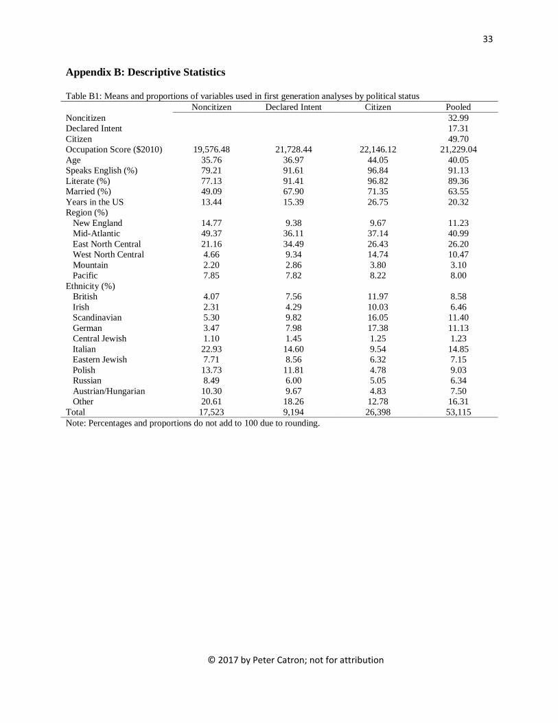
naturalized in 1902). Descriptive statistics of the dependent and independent variables are

described in Appendix B.

Second Generation Outcomes

The above analyses establish whether there was a citizenship advantage in the labor

market for the first generation, but it remains unknown whether this advantage transferred to

their children. To assess the effects of parental citizenship on second generation outcomes, I use

a new panel dataset that follows individuals from their childhood household in 1920 to when

they were participating in the labor force in 1940. I match individuals between US censuses by

first and last name, age, and state of birth; details on the matching procedure are provided in

Appendix C. I restrict my attention to second generation male children who had European-born

parents and were between the ages of 5 and 18 in the one-percent 1920 census (Ruggles et al.

2010).3 The purpose of not matching those who are younger than 5 years old is because

mortality is unequally distributed in these younger ages and this may bias estimates through

matching by introducing selectivity at some levels but not others. These matched individuals are

also young in 1940 (between the ages of 20 and 24) when the outcomes analyzed in this paper,

years of education and labor market outcomes, are still in process. All matched children were

born in the US.

3 The purpose of using the one-percent 1920 sample instead of the full-count census is because citizenship was not digitized as of the beginning of this project.

16


The sample is restricted to those who are living with at least one parent in 1920. Keeping

those who are living with at least one parent is because parent’s citizenship status must be

inferred from the POPLOC and MOMLOC variables available from IPUMS (Ruggles et al.

2010). Not living with a parent reflects class (see Bodner 1985) and this may have implications

to the extent that citizenship reflects social class.4 However, because we cannot infer citizenship

status of children without parents, nor any other family variables, these children are omitted from

the analyses. Thus, the second generation is defined as a child living with a foreign-born father.

In single-mother households, however, a child is defined as second generation if his mother was

born outside the US. The focus on children’s father is because household citizenship status

during this era was dependent on men. Before 1922, when the Cable Act was signed into law,

women took their husband’s citizenship status even if they were born in the US. During this era,

there were no mixed status families as there are today since parent’s citizenship status was the

same.

Table 1 presents the match rates along various dimensions in the panel dataset. My

matching procedure generates a final sample size of 12,051 second generation children where I

successfully match 45 percent of children forward from 1920 to 1940. This match rate is slightly

higher than the standard for historical matched samples (e.g. Abramitzky et al. 2012).5 More

details on matching are found in Appendix C.

4 Children who do not live with their parent, but were successfully matched in the dataset, have on average fewer years of education in 1940 than children of noncitizens, intending citizens, and citizens. The age distribution of those who did not live with at least one parent is skewed such that most were in their teens and 42 percent were between the ages of 16 and 18. Of the 466 matched second generation children who were not living with their parents, fifteen percent had fathers born in Ireland, fourteen percent in Italy, and eighteen percent in Germany. The rest had parents born throughout the rest of Europe. 5 Factors that contribute to higher match rates in the 1940 Census include better transcription, a more literate population who are better able to report their name and age more accurately over

17


[TABLE 1 HERE]

While sons with uncommon names are more likely to match between census years, the

matched sample is reasonably representative of the population. Sons in the matched sample in

Table C1 in Appendix C show that they are close to a representative sample in 1940 on

educational attainment and income. Second generation children in the matched sample had an

average of .36 more years of education and earned 8.41 1940 dollars less than those in the

representative sample. However, the match rates in Table 1 suggest that the probability of being

linked is likely correlated with parental citizenship status: 31 percent of children of noncitizens

matched while 46 percent of children of citizens matched. In part, the lower match rate of

noncitizens reflects return migration where parents took their children back to Europe. This

article, therefore, is about the second generation who stayed in the US. As a sensitivity check, I

ran each analysis below for the pooled samples by reweighting the panel sample to reflect the

actual distribution of father’s country of origin in the 1940 population. Results change at the

third decimal place, reported in Appendix C, but do not substantively change any conclusions.

To analyze the intergenerational citizenship advantage, I focus on three outcome

variables for second generation children separately. First, I focus on the number of years of

education because it often explains labor market outcomes and is an important factor for

immigrant incorporation (Bean et al. 2011). Second, I focus on income, measured as the

respondent’s pre-tax wage and salary income received in the previous year as an employee.

The control variables used to predict the second generation’s social destination include a

number of individual and family characteristics that are straightforward: child’s age and age-

squared, parent’s age and age-squared, parent’s years in the US and years in the US-squared,

time, and improvements in life expectancy. Younger samples also tend to match better since there are lower mortality rates than in adult samples.

18


dummies for metropolitan status as defined in the first generation analyses, and region. I also

control for parent’s English ability and literacy as rough proxies for parental education level as

mentioned above. Since children come from different family structures that may influence their

later attainment, I also include a dummy category for whether the child lived in a single father

household and a dummy for whether the child lived with both parents compared to a reference

category of living in a single mother household. Almost all of the parents in the both parents

category report being married to each other. I do not control for parental occupation in these

analyses because it is impossible to know occupations prior to citizenship attainment.6 All

control variables are measured in the 1920 one-percent sample. Descriptive statistics of the

control variables are presented in Appendix B.

Similar to the first generation analyses, child’s outcomes are riddled with selection where

parent’s political status may correlate with other variables that will allow children to do better in

life whether or not his parents have naturalized. Above, this was corrected for by comparing

citizens with intending citizens since both categories were likely similar with the exception of

political status. Thus, the gap between these two groups provided the citizenship advantage in

occupational outcomes for the first generation. However, the difference between children of

citizens and children of intending citizens may not represent the intergenerational citizenship

advantage. This is because there is no guarantee that children of those who declared intent had

no parent citizenship years in their life course. Analogous to an event history setup, parental

political status is right censored in 1920 (i.e. we do not know about political status after this

year). Since many intending citizens naturalized, children may have grown up with a citizen

parent, which is unknown in the analyses. For instance, if an intending citizen had a five year

6 Inclusion of parents’ occupation in the models does not substantively change any results.

19


old child in 1920 and then naturalized after their citizenship status was recorded in the census,

the child grew up with a citizen parent and thus would have benefited from the citizenship

advantage.7 Because of the likelihood of children of intending citizens growing up as children of

citizens, I change the reference category to children of noncitizens. This comparison gives the

total effect of the intergenerational citizenship advantage.

To analyze children’s social destinations, therefore, I fit the following model: where represents the outcome variable (either years of education or the natural log of income)

for individual i, is a vector of control variables noted above; is a dummy variable

(1,0) if the child’s parent has declared intent in 1920 and is a dummy variable (1,0) if the

child’s parent is a citizen in 1920 compared to a reference category of if the child’s parent is a

noncitizen. As with the first generation analyses, I estimate the above model separately for each

ethnic group defined in Appendix A and a pooled sample of all ethnicities.

In addition to understanding the intergenerational citizenship advantage, I also test the

timing of citizenship acquisition based on when the parent naturalized and when the child was

born. To do this, I limit the matched sample to children of citizens and generate three dummy

categories: parent naturalized when the child was 0 to 5; parent naturalized when the child was 6

to 12; parent naturalized when the child was a teenager; compared to a reference category of

parent naturalized before the child was born. Controlling for the above variables, these analyses

will point to whether growing up with a citizen parent matters compared to having a parent

naturalize late.

7 In a separate matched sample of foreign-born men over the age of 25 using the same methods described in this paper, I find that nearly 80 percent of intending citizens in the 1920 one-percent sample have become naturalized by 1940. This sample is not representative of parents in the children’s sample, but it suggests that most followed through to citizenship.

20


Results

First Generation Outcomes

My analyses begin by providing estimates of the relative citizenship advantage for the

first generation by ethnicity. Each analysis is restricted by ethnic group. Thus, the British

noncitizen coefficient in Figure 2 reports the difference in occupation-based income between

noncitizens and those who declared intent among individuals who were born in Britain. The

pooled sample in the last row includes all immigrants from Europe, controlling for ethnicity. As

mentioned, I interpret a negative coefficient of noncitizens as evidence for positive selection into

citizenship and a positive coefficient of citizenship as evidence for the citizenship advantage.

The results are presented in 2010 dollars for ease of interpretation.

Figure 2 reports that in all cases, noncitizens had a lower occupation-based income

compared to intending citizen counterparts, all else equal. This suggests positive selection into

citizenship for all groups. However, not all groups show behaviors equally. Italians and Eastern

Jews betray the lowest, albeit statistically significant, gap between noncitizens and intending

citizens. Noncitizen Italians had $896 lower occupation-based income than Italian intending

citizens. Similarly, noncitizen Eastern Jews had $1,185 lower occupation-based income ceteris

paribus intending citizens. Irish and Central Jews report the largest gap between noncitizens and

intending citizens: Irish noncitizens had roughly $1800 occupation-based income lower than

Irish intending citizens and Central Jewish noncitizens had over $2,000 lower occupation-based

income. Thus, part of the citizenship advantage is due to selection where immigrants who happen

to naturalize also likely perform better in the labor market even if they do not naturalize.

21


While there was positive selection into citizenship, there is also evidence for a citizenship

advantage in occupational income. All groups show a positive and significant coefficient

comparing citizens with those who declared intent, with the exception of the British. At the low

end, Italian citizens had an occupation-based income of $464 more than Italian intending

citizens. This may reflect Italian concentration in sectors like construction that were less

affected by the policies mentioned above. It may also reflect the role of ethnic enclaves that may

protect noncitizens and aid in their upward occupational mobility without need to obtain

citizenship (Bailey and Waldinger 1991). Because of sample sizes in some of the locals, the role

of the composition of the local population and citizenship should be looked at using the full-

count 1920 census in future research.

Other groups that often concentrated in sectors that were more susceptible to the above

policies and likely experienced greater discrimination in the workforce, such as Slavs, held a

high citizenship advantage. For instance, Russian citizens had an occupation-based income of

$1,739 more than Russian intending citizens, while the Polish citizen citizenship advantage was

roughly $1,200 more than Polish intending citizens. This effect likely reflects signaling where

groups that were heavily discriminated against due to their perceived unassimilability are able to

show that they are becoming similar to their American countrymen. Given the societal reception

of these groups and their industrial concentration, the value of citizenship was greater for these

Eastern Europeans. Public and private employers would reward citizenship for members of these

groups due to the social forces mentioned above and this is reflected in the Eastern European

citizenship advantage in Figure 2. By contrast, groups that may have been treated as members

without the need for formal citizenship, such as the British, do not report a high nor statistically

22


significant citizenship advantage. British immigrants likely did not need to prove their

membership to employers and thus experienced better occupations without formal citizenship.

Other groups, such as the Irish, also report a large citizenship advantage. Here, we may

be seeing the economic impact of political mobilization. The importance of government as an

important historical lever of upward attainment for Irish immigrants during this time was

famous: government was a chief locus of employment for Irish immigrants, who, along with

their descendants, carved up its functions into a series of ethnic strongholds; it steered contracts,

and through contracts jobs, to its ethnic political backers; and it provided services for those

ethnics whom it could not furnish with jobs. Irish immigrants who became citizens likely

benefited disproportionately from this process since they could vote and hold public jobs.

Although it is impossible to know the specific reasons individuals in the census became citizens,

future research should understand the role of different avenues into citizenship that would lead to

different outcomes. Nevertheless, the gap between citizens and those who have declared intent

suggests that there was a citizenship premium over and above the positive selection into this

variable mentioned above. The pooled sample suggests that the citizenship advantage was

roughly $1,073 during this period.

[FIGURE 2 HERE]

Although the analyses in Figure 2 control for years in the US, however, intending citizens

who have been in the US for many years may be fundamentally different than those who

declared intent earlier. Intending citizens who declared late may have had financial

considerations, problems learning English, or any other feature that may have limited their

ability to obtain this status. This may positively bias the citizenship advantage by comparing

citizens to immigrants who intended late. Figure 3 reports the average occupation-based income

23


of the three political categories by years in the US. The years in the US past 40 are not reported

since few intending citizens and noncitizens had been in the US for this long. As shown,

intending citizens remain a steady middle group as the number of years in the US increases.

However, there is a growing gap between intending citizens and citizens the longer immigrants

have remained in the US. In part, this reflects the differences in individuals who intend late and

in part the advantages citizenship accrues over time as discussed below. As a sensitivity test, I

also ran each regression for only those who have been in the US for fewer than 20 years and

again for fewer than 10 years. Results of the pooled sample report that the citizenship advantage

is higher (approximately $1,200 occupation-based income) than in Figure 2 when limiting the

sample to those who have been in the US for 5 to 20 years, but lower (roughly $500) when

limiting the sample to those who have been in the US for 5 to 10 years.

[INSERT FIGURE 3 HERE]

The citizenship advantage may not have been instantaneous, however, but rather gradual.

The 1920 census is unique in that it is the only census during this period to ask citizens when

they naturalized. I therefore supplement the above analyses by analyzing the citizenship

advantage based on the number of years since naturalization. This analysis reports the

immediate and near immediate effects of citizenship as well as whether the citizenship advantage

increases the longer an individual has been naturalized. The results report each ethnicity

separately and for a pooled sample. As with the above analysis, the four citizenship categories

are compared to an intending citizen reference.

As shown in Table 2, there is no statistically substantive effect of citizenship for those

who have recently naturalized (0-5 years) vis-à-vis intending citizens in all ethnic samples with

the exception of the Polish. By contrast, in all samples, immigrants who have been naturalized

24


for more than sixteen years report large economic advantages compared to their intending citizen

counterparts: British immigrants had an occupational income score of just over $1,000 while

Austrian/Hungarian immigrants had an occupational income score of over $3200. In some cases,

the earnings advantage for citizens falls for those who naturalized between 11 and 15 years prior

to 1920. This likely reflects the impact of 1906 legislation that made it harder for immigrants to

obtain citizenship (Bloemraad 2006). Nevertheless, the growing earnings advantage suggests

that citizenship allowed for access to promotion lines that moved them into higher occupational

positions over time. When understanding the consequences of citizenship, therefore, it is

important to understand the accrual of the citizenship advantage and not only whether an

immigrant is a citizen. Because of this, the timing between when immigrants naturalize and

when their children are born may have important consequences on second generation outcomes.

[TABLE 2 HERE]

Second Generation Outcomes

As shown, naturalized immigrants enjoyed better occupational outcomes than their

noncitizen counterparts. The following analyses seek to understand whether this advantage

transferred to their children once they enter the labor market. I begin by first reporting the

differences between children of citizens and intending citizens versus children of noncitizens for

a pooled sample. These analyses allow us to understand how children fared in the labor market

compared to one another based on parental political status as well as other factors that influence

intergenerational mobility. Model 1 of Table 3 reports that children of citizens had over six

months more education compared to their noncitizen counterparts without any other control

25


variables. By contrast, children of intending citizens had over three months more education

compared to the same reference group. These initial results suggest that second generation

outcomes were linked to parents’ political status. However, the gap between second generation

groups slightly shrinks as relevant control variables are added. Children of citizens have about

half a year more education than their noncitizen counterparts while children of intending citizens

show no substantively statistical difference. These results point to an intergenerational

citizenship advantage where children with citizen parents remained in school longer than their

noncitizen counterparts.

While the first two models of Table 3 test differences in educational attainment, models 3

through 8 test differences in labor market outcomes. Model 3 reports that children of citizens

have 11 percent higher income in 1940 dollars than children of noncitizens without controlling

for any other variables. The intergenerational citizenship advantage continues where children of

citizens hold six percent higher earnings once more control variables are added including

parent’s literacy and parent’s English ability. These income differences are important to note

because the 1940s, when income is measured, was a period of great wage compression (Goldin

and Margo 1992). Indeed, the compressed wage structure has been cited as one component that

produced assimilation among the second generation and the native-born during this era (Alba

and Nee 2001). Thus, any statistical differences in income between groups are important since

they represent unequal outcomes based on different political statuses. A similar effect emerges

when predicting occupational income. Children of citizens have an occupational income score of

more than $600 than their noncitizen counterparts suggesting that citizenship attainment allowed

their children to move up the occupational hierarchy.

26


Models 5 and 8 in Table 3, however, report that the citizenship advantage has no

statistically substantive effect on income once educational attainment is added to the analyses.

This suggests that the intergenerational citizenship advantage does not operate over and above its

influence on educational attainment. However, the return to one year of education on income for

the second generation during this time is over seven percent. As shown in model 2, having a

citizen parent raises children’s educational attainment by about half a year. Thus, through its

impact on educational attainment, the citizenship advantage raises individual income by about

four percent. The additional income received by the second generation each year through its

influence from educational attainment will have a cumulative effect allowing for greater wealth

attainment over time. Thus, the intergenerational citizenship advantage has an important

influence through educational attainment that then has an important influence on children’s later

labor market experiences.

[TABLE 3 HERE]

Figure 4 presents differences between children of citizens and noncitizens by ethnicity.

For the remaining analyses, I focus on educational attainment given large effect citizenship

exerts on this outcome. Each analysis in Figure 4 is run by restricting the sample to each ethnic

subgroup. Thus, as in the first generation analyses, the British coefficients report the difference

between children of citizens and noncitizens among those of British descent. Every analysis

controls for the same variables as reported in model 2 of Table 3.

Figure 4 reports that the intergenerational citizenship advantage has different effects

depending on child’s ethnicity. Children with parents born in Western Europe do not report any

statistically substantive difference between parental political statuses. These groups, however,

also held the lowest citizenship advantage in the first generation analyses reported in Figure 2.

27


While the first generation analyses in Figure 2 are not representative of the parental sample in

Figure 4 since fertility rates differ across individuals and groups (Duncan 1966), the low impact

of citizenship on later outcomes likely reflects Western Europeans being treated as members

since they were often viewed as contributors to America’s system of values and economy.8

However, all Slavic and Jewish groups report strong intergenerational citizenship effects.

However, the central Jewish coefficients are likely high due to low sample size rather than a

strong citizenship advantage since the coefficients from Figure 2 are also low for this group.

Children of both Polish and Russian immigrants enjoy over one year of education if their parent

had naturalized compared to if their parent had not naturalized, all else equal. Similarly, children

of Italians have over four months education than their noncitizen counterparts. These results

suggest that citizenship was particularly important for eastern European groups.

[FIGURE 4 HERE]

The final analyses seek to test whether the intergenerational citizenship advantage should

be understood as a binary or continuous measure. As shown above, the citizenship advantage

allowed for greater wage growth the longer an individual had been naturalized. This suggests

that the citizenship advantage is not immediate, but rather gradual. The growth of the citizenship

advantage likely strengthens the family economy, which then allows children to stay in school

longer instead of entering the workforce early. Thus, the timing of parental citizenship based on

when the child was born likely matters where we would expect children who grow up with a

citizen parent to do better in educational attainment than a child with a parent who naturalized

when he was older. The following analysis limits the pooled sample to children with a citizen

parent. I separate children based on when their parent naturalized and predict years of education

8 For instance, some individuals have no children and they are thus not included in the model, while others have many children and have a higher chance of being included multiple times.

28


controlling for the variables mentioned above. I do not report the effects by ethnicity due to low

cell counts in some categories.

As shown in Table 4, there is no statistically substantive difference between children with

parents who naturalized before they were born and children with parents who naturalized when

they were young. However, children with parents who naturalized as a teenage have over seven

months less education compared to children who have parents who naturalized before they were

born. This result suggests that early naturalization allowed for greater investments in children,

which allowed them to remain in school longer. These investments may include early childhood

health investments or early schooling investments that allowed children to obtain more

schooling. Children of parents who naturalized when they were teenagers had fewer citizenship

years and likely dropped out of school early to help support the family economy. Given the large

effect of education on income for this group, however, those with fewer years of education

performed worse in the labor market when they were adults. Nevertheless, this effect suggests

that the consequences of citizenship are not only a binary measure, but also a continuous one.

[TABLE 4 HERE]

Discussion/Conclusion

This article examined a question that has been ignored until now: did parental citizenship

acquisition affect intergenerational attainment? Avoidance of this question reflects a

perspectival blinder that citizenship acquisition had few if any subsequent effects outside of the

right to vote. However, citizenship is an institution of exclusion, not just inclusion, giving

unequal rights and entitlements to citizens and noncitizens. This gap widened in the first half of

the twentieth century through state, local, and employer policies that produced different

29


outcomes for both the first and second generation depending on political status. This article,

therefore, is the first to uncover this relationship by being the first sociological research to track

individuals across US censuses. While the dominant accounts of assimilation do not take into

consideration the role of parental citizenship attainment during this era (Alba and Nee 2003;

Portes and Rumbaut 2001), this article suggests that immigrant intergenerational attainment was

linked to macro-level political processes.

Laws and employer practices barred noncitizens from certain occupations and public

employment. These practices had long term consequences for immigrant populations and their

children. Citizens’ occupation-based income was $400 to $1,700 greater than intending citizens

in 1920 pointing to a strong citizenship advantage in occupation outcomes. However, the

citizenship advantage was not immediate for the first generation, but rather accrued over time.

The first generation who had been naturalized between zero and five years had an occupation-

based income of roughly $500 more than their intending citizen counterparts while immigrants

who have been naturalized for over 16 years had an occupation-based income of over $1,800.

These results are the first to uncover the occupational advantage in citizenship acquisition during

this era and they suggest that citizenship was a requirement to achieve greater wage growth and

occupational attainment.

The citizenship advantage, however, also had an intergenerational effect. While there

was steady upgrading of second generation educational and occupational outcomes during this

era (Lieberson 1980), there were also important differences based on first generation political

statuses. Parents who became citizens had more resources to invest in their children, which

allowed for higher educational attainment. For some immigrant groups, namely those from

eastern Europe, had an intergenerational citizenship advantage of over a year more education.

30


Through the strong influence of education on income, children performed better in the labor

market as a result of their parent being a citizen. However, the positive benefits of parental

citizenship depended on the timing of citizenship acquisition and child’s birth. Children who

grew up with citizen parents were more likely to have greater educational attainment than

children with parents who naturalized when they were teenagers net of parents years spent in the

US. The increased resources associated with citizenship acquisition likely allowed parents to

provide a more attractive home environment that was not available to children with parents who

naturalized late or never naturalized.

The effects of citizenship, however, were not uniform across groups: eastern Europeans

benefited the most from citizenship acquisition. The influence of citizenship likely interacts with

the context of reception in the receiving society, the endogenous contextual influences deriving

from the society of origin, and the size and type of migration flow. Thus, the policies that

promoted citizens to better occupations were often targeted at southern and eastern European

immigrant groups as opposed to Western Europeans. However, the groups who gained most

from citizenship acquisition were also the groups least likely to naturalize (Bloemraad 2006).

While this article focuses on the aggregate effect of citizenship for immigrant groups in the

country, the salience of citizenship may have been greater in some areas given other contextual

features. These features may occur at the state, county, or firm level. Future research that takes

advantage of a full-count 1920 census (as opposed to the 1% 1920 census used in this article)

matched to the full-count 1940 census once citizenship is digitized should test mechanisms

leading to varying economic benefits for citizenship acquisition by geography.

Nevertheless, understanding the citizenship advantage of immigrants in the past also

helps us understand current events. Present day trends are a continuation of a pattern put in place

31


in the early 20th century, both impeding access to citizenship and widening formal inequalities

between citizens and noncitizens. As noted, the growing restriction at the border had led to both

the proliferation of undocumented immigration, which means that the population of persons

ineligible for citizenship has grown. Moreover, for the eligible, the barriers to citizenship

acquisition began to climb in the late 1980s, with the result that a large portion of the legally

resident population eligible to naturalize does not. As a result – especially due to 1990s

legislation – noncitizens, regardless of legal status, are increasingly vulnerable to deportation,

with numbers rising in recent years. Although researchers have largely ignored citizenship’s role

in producing occupational attainment, its effect is likely larger for today’s immigrants who must

undergo many statuses and expense to achieve this outcome (Bean, Brown, Bachmeier 2015).

This article argues that there are important effects of citizenship acquisition for both the

first and second generations. Researchers often point to the past and then determine whether

today’s immigrants will follow a similar trajectory. However, little is known about how

yesterday’s immigrants achieved upward attainment. This paper argues that citizenship was one

way immigrants made it in America. While more research is needed to understand the sources of

within-immigrant group differences, the availability of newly research digitized data of full-

count censuses, naturalization records, and passenger files allow researchers to understand these

processes in depth. Although sociologists have neglected these rich data sources, the availability

of longitudinal data that is not available for today’s immigrants will provide important insight

into the immigrant experience.

32


Appendix A: Coding for Ethnicity As described in the text, different groups that are of sociological interest came from the same national origins during this era. It is therefore necessary to separate groups based on their birthplace and mother tongue. In the first generation analyses, I use the individual’s birthplace and mother tongue coded in Table A1. However, in the second generation analyses, I code each ethnicity based on his parent’s birthplace and mother tongue. The codes are presented in Table A1. Table A1: Ethnicity of parent

Ethnicity Description Irish, Italian Born in respective countries British Born in England, Scotland, or Wales Scandinavian Born in Iceland, Norway, Sweden, or Denmark German Born in Germany or Germany-Poland and mother tongue is

German Central European Jewish Born in Central Europe and mother tongue is Yiddish Eastern Jewish Born in Eastern Europe and mother tongue is Yiddish Polish Born in Eastern or Central Europe and mother tongue is Polish Other Those not described above

33


Appendix B: Descriptive Statistics Table B1: Means and proportions of variables used in first generation analyses by political status Noncitizen Declared Intent Citizen Pooled Noncitizen 32.99 Declared Intent 17.31 Citizen 49.70 Occupation Score ($2010) 19,576.48 21,728.44 22,146.12 21,229.04 Age 35.76 36.97 44.05 40.05 Speaks English (%) 79.21 91.61 96.84 91.13 Literate (%) 77.13 91.41 96.82 89.36 Married (%) 49.09 67.90 71.35 63.55 Years in the US 13.44 15.39 26.75 20.32 Region (%) New England 14.77 9.38 9.67 11.23 Mid-Atlantic 49.37 36.11 37.14 40.99 East North Central 21.16 34.49 26.43 26.20 West North Central 4.66 9.34 14.74 10.47 Mountain 2.20 2.86 3.80 3.10 Pacific 7.85 7.82 8.22 8.00 Ethnicity (%) British 4.07 7.56 11.97 8.58 Irish 2.31 4.29 10.03 6.46 Scandinavian 5.30 9.82 16.05 11.40 German 3.47 7.98 17.38 11.13 Central Jewish 1.10 1.45 1.25 1.23 Italian 22.93 14.60 9.54 14.85 Eastern Jewish 7.71 8.56 6.32 7.15 Polish 13.73 11.81 4.78 9.03 Russian 8.49 6.00 5.05 6.34 Austrian/Hungarian 10.30 9.67 4.83 7.50 Other 20.61 18.26 12.78 16.31 Total 17,523 9,194 26,398 53,115 Note: Percentages and proportions do not add to 100 due to rounding.

34


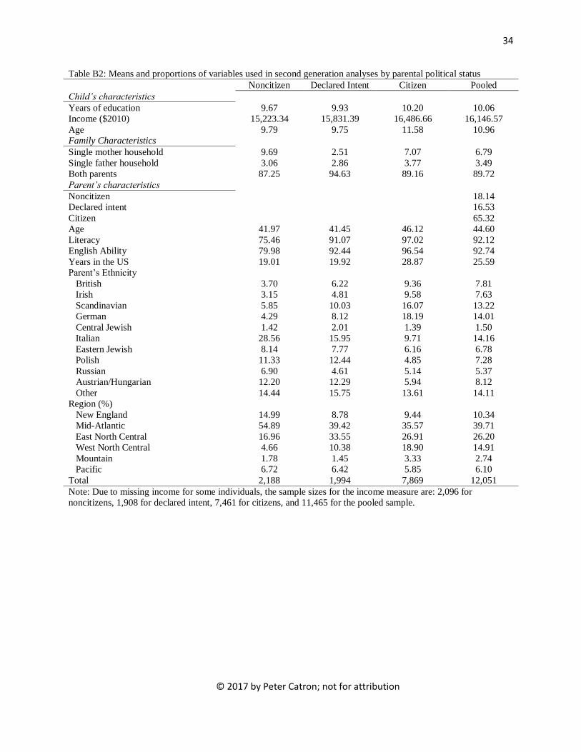
Table B2: Means and proportions of variables used in second generation analyses by parental political status Noncitizen Declared Intent Citizen Pooled Child’s characteristics Years of education 9.67 9.93 10.20 10.06 Income ($2010) 15,223.34 15,831.39 16,486.66 16,146.57 Age 9.79 9.75 11.58 10.96 Family Characteristics Single mother household 9.69 2.51 7.07 6.79 Single father household 3.06 2.86 3.77 3.49 Both parents 87.25 94.63 89.16 89.72 Parent’s characteristics Noncitizen 18.14 Declared intent 16.53 Citizen 65.32 Age 41.97 41.45 46.12 44.60 Literacy 75.46 91.07 97.02 92.12 English Ability 79.98 92.44 96.54 92.74 Years in the US 19.01 19.92 28.87 25.59 Parent’s Ethnicity British 3.70 6.22 9.36 7.81 Irish 3.15 4.81 9.58 7.63 Scandinavian 5.85 10.03 16.07 13.22 German 4.29 8.12 18.19 14.01 Central Jewish 1.42 2.01 1.39 1.50 Italian 28.56 15.95 9.71 14.16 Eastern Jewish 8.14 7.77 6.16 6.78 Polish 11.33 12.44 4.85 7.28 Russian 6.90 4.61 5.14 5.37 Austrian/Hungarian 12.20 12.29 5.94 8.12 Other 14.44 15.75 13.61 14.11 Region (%) New England 14.99 8.78 9.44 10.34 Mid-Atlantic 54.89 39.42 35.57 39.71 East North Central 16.96 33.55 26.91 26.20 West North Central 4.66 10.38 18.90 14.91 Mountain 1.78 1.45 3.33 2.74 Pacific 6.72 6.42 5.85 6.10 Total 2,188 1,994 7,869 12,051 Note: Due to missing income for some individuals, the sample sizes for the income measure are: 2,096 for noncitizens, 1,908 for declared intent, 7,461 for citizens, and 11,465 for the pooled sample.

35


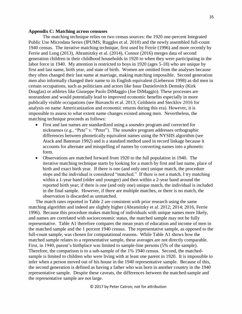
Appendix C: Matching across censuses The matching technique relies on two census sources: the 1920 one-percent Integrated Public Use Microdata Series (IPUMS; Ruggles et al. 2010) and the newly assembled full-count 1940 census. The iterative matching technique, first used by Ferrie (1996) and more recently by Ferrie and Long (2013), Abramitzky et al. (2014), Connor (2016) merges data of second generation children in their childhood households in 1920 to when they were participating in the labor force in 1940. My attention is restricted to boys in 1920 (ages 5-18) who are unique by first and last name, birth year, and state of birth. Women are omitted from the analyses because they often changed their last name at marriage, making matching impossible. Second generation men also informally changed their name to its English equivalent (Lieberson 1998) as did men in certain occupations, such as politicians and actors like Issur Danielovitch Demsky (Kirk Douglas) or athletes like Giuseppe Paolo DiMaggio (Joe DiMaggio). These processes are nonrandom and would potentially lead to improved economic benefits especially in more publically visible occupations (see Biavaschi et al. 2013; Goldstein and Stecklov 2016 for analysis on name Americanization and economic returns during this era). However, it is impossible to assess to what extent name changes existed among men. Nevertheless, the matching technique proceeds as follows: First and last names are standardized using a soundex program and corrected for

nicknames (e.g., “Pete” v. “Peter”). The soundex program addresses orthographic differences between phonetically equivalent names using the NYSIIS algorithm (see Atack and Bateman 1992) and is a standard method used in record linkage because it accounts for alternate and misspelling of names by converting names into a phonetic form. Observations are matched forward from 1920 to the full population in 1940. The iterative matching technique starts by looking for a match by first and last name, place of birth and exact birth year. If there is one (and only one) unique match, the procedure stops and the individual is considered “matched.” If there is not a match, I try matching within a 1-year band (older and younger) and then within a 2-year band around the reported birth year; if there is one (and only one) unique match, the individual is included in the final sample. However, if there are multiple matches, or there is no match, the observation is discarded as unmatched.

The match rates reported in Table 2 are consistent with prior research using the same matching algorithm and indeed are slightly higher (Abramitzky et al. 2012; 2014; 2016, Ferrie 1996). Because this procedure makes matching of individuals with unique names more likely, and names are correlated with socioeconomic status, the matched sample may not be fully representative. Table A1 therefore compares the mean years of education and income of men in the matched sample and the 1 percent 1940 census. The representative sample, as opposed to the full-count sample, was chosen for computational reasons. While Table A1 shows how the matched sample relates to a representative sample, these averages are not directly comparable. First, in 1940, parent’s birthplace was limited to sample-line persons (5% of the sample). Therefore, the comparison is to a sub-sample of the 1% 1940 census. Second, the matched-sample is limited to children who were living with at least one parent in 1920. It is impossible to infer when a person moved out of his house in the 1940 representative sample. Because of this, the second generation is defined as having a father who was born in another country in the 1940 representative sample. Despite these caveats, the differences between the matched-sample and the representative sample are not large.

36


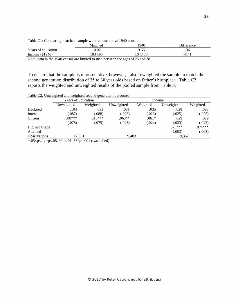
Table C1: Comparing matched-sample with representative 1940 census Matched 1940 Difference Years of education 10.02 9.66 .36 Income ($1940) 1034.95 1043.36 -8.41 Note: data in the 1940 census are limited to men between the ages of 25 and 38 To ensure that the sample is representative, however, I also reweighted the sample to match the second generation distribution of 25 to 38 year olds based on father’s birthplace. Table C2 reports the weighted and unweighted results of the pooled sample from Table 3. Table C2: Unweighted and weighted second generation outcomes Years of Education Income Unweighted Weighted Unweighted Weighted Unweighted Weighted Declared Intent

.104 (.087)

.093 (.088)

.031 (.026)

.035 (.026)

.028 (.025)

.033 (.025)

Citizen .508*** (.078)

.510*** (.079)

.063** (.023)

.061* (.024)

.029 (.023)

.029 (.023)

Highest Grade Attained

.075*** (.003)

.074*** (.003)

Observations 12,051 9,483 9,362 +.05<p<.1, *p<.05, **p<.01, ***p<.001 (two-tailed)

37


References

Abramitzky, Ran, Leah Boustan, and Katherine Eriksson. 2014. “A Nation of Immigrants:

Assimilation and Economic Outcomes in the Age of Mass Migration.” Journal of

Political Economy 122(3): 467-506

Alba, Richard and Victor Nee. 2003. Remaking the Mainstream: Assimilation and

Contemporary Immigration. Cambridge: Harvard University Press.

Atack, Jeremy, and Fred Bateman. 1992. “’Matchmaker, Matchmaker, Make Me a Match’: A

General Personal Computer-Based Matching Program for Historical Research.”

Historical Methods 25(2): 53-65.

Barrett, James R. 1992. “Americanization from the Bottom Up: Immigration and the Remaking

of the Working Class in the United States, 1880-1930.” The Journal of American History

79(3): 996-1020.

Bean, Frank D., Mark a. Leach, Susan K. Brown, James D. Bachmeier, and John R. Hipp. 2011.

“The Educational Legacy of Unauthorized Migration: Comparisons Across U.S.

Immigrant Groups in How Parents’ Status Affects Their Offspring.” International

Migration Review 45(2): 348-385.

Bean, Frank D., Susan K. Brown, and James D. Bachmeier. 2015. Parents Without Papers: The

Progress and Pitfalls of Mexican American Integration The Russell Sage Foundation

Bernard, William S. 1936. “Cultural Determinants of Naturalization.” American Sociological

Review 1:943-53.

Biavaschi, Costanza, Corrado Giulietti, and Zahra Siddique. 2013. “The Economic Payoff of

Name Americanization.” IZA Discussion Paper Series No. 7725.

38


Bloemraad, Irene. 2002. “The North American Naturalization Gap: An Institutional Approach to

Citizenship Acquisition in the United States and Canada.” International Migration

Review 36(1): 194-229.

Bloemraad, Irene. 2006. “Citizenship Lessons from the Past: The Contours of Immigrant

Naturalization in the Early 20th Century.” Social Science Quarterly 87(5): 927-953.

Bratsberg, Bernt, James F. Ragan, Jr., and Zafar M. Nasir. 2002. “The Effect of Naturalization

on Wage Growth: A Panel Study of Young Male Immigrants.” Journal of Labor

Economics 20(3): 568-597.

Bodner, John. 1985. The Transplanted: A History of Immigrants in Urban America.

Bloomington: Indiana University Press.

Catron, Peter. 2016. “Made in America? Immigrant Occupational Mobility in the First Half of

the Twentieth Century.” American Journal of Sociology 122(2): 325-378.

Connor, Dylan Shane. 2016. “The Cream of the Crop? Inequality and Selectivity in Ireland

during the Age of Mass Migration.” California Center for Population Research Working

Paper

Duncan, Otis Dudley. 1966. “Methodological Issues in the Analysis of Social Mobility.” Pp. 51-

97 in N.J. Smelser and S.M. Lipset (eds.), Social Structure and Mobility in Economic

Development. Chicago: Aldine.

Ferrie, Joseph P. 1996. “A New Sample of Males Linked from the Public Use Micro Sample of

the 1850 U.S. Federal Census of Population to the 1860 U.S. Federal Census Manuscript

Schedule.” Historical Methods 29(4): 141-156.

39


Ferrie, Joseph P., and Jason Long. 2013. “Intergenerational Occupational Mobility in Great

Britain and the United States since 1850.” American Economic Review 103(7): 1109-

1137.

Fields, Harold. 1933. “Where Shall the Alien Work?” Social Forces. 213-221

Fields, Harold. 1935. “Conflicts in Naturalization Decisions.” Temp. LQ 10: 272

Fischer, Claude S. and Michael Hout. 2006. Century of Difference: How America Changed in

the Last One Hundred Years. New York: Russell Sage Foundation.

FitzGerald, David and David Cook-Martin. 2014. Culling the Masses: The Democratic Origins

of Racist Immigration Policy in the Americas. Harvard University Press

Fox, Cybelle, and Irene Bloemraad. “Beyond ‘White by Law’: Explaining the Gulf in

Citizenship Acquisition between Mexican and European Immigrants, 1930.” Social

Forces 94(1): 181-207.

Gavit, John Palmer. 1922. Americans by Choice. New York: Harper and Brothers.

Gerstle, Gary and John Mollenkopf. 2001. E Plubribus Unum? Contemporary and Historical

Perspectives on Immigrant Political Incorporation. New York: Russell Sage Foundation.

Goldin, Claudia, and Robert A. Margo. 1992. “The Great Compression: The Wage Structure in

the United States at Mid-Century.” Quarterly Journal of Economics 107(1): 1-34.

Goldstein, Joshua R. and Guy Stecklov. 2016. “From Patrick to John F. Ethnic Names and

Occupational Success in the Last Era of Mass Migration.” American Sociological Review

Gosnell, Harold F. 1928. “Non-Naturalization: A Study in Political Assimilation.” American

Journal of Sociology 33: 930-39.

Gosnell, Harold F. 1929. “Characteristics of the Non-Naturalized.” American Journal of

Sociology. 34:847-55.

40


Gosnell, Harold F. 1937. Machine Politics: Chicago Model. Chicago: University of Chicago

Press.

Lieberson, Stanley. 1980. A Piece of the Pie: Blacks and White Immigrants since 1880.

Berkeley: University of California Press.

Loizides, Georgios Paris. 2007. “’Making Men’ at Ford: Ethnicity, Race, and Americanization

During the Progressive Period.” Michigan Sociological Review 21: 109-148.

Menjivar, Cecilia, and Leisy Abrego. 2012. “Legal Violence: Immigration Law and the Lives of

Central American Immigrants.” American Journal of Sociology 117(5): 1380-1421

Motomura, Hiroshi. 2006. Americans in Waiting: The Lost Story of Immigration and Citizenship

in the United States. Oxford University Press.

Ngai, Mae. 2004. Impossible Subjects: Illegal Aliens and the Making of Modern America.

Princeton University Press.

Pagnini, Deanna L. and S. Philip Morgan. 1990. “Intermarriage and Social Distance Among U.S.

Immigrants at the Turn of the Century.” American Journal of Sociology 96(2): 405-432.

Perlmann, Joel. 2005. Italians Then, Mexicans Now: Immigrant Origins and Second

Generation Progress, 1890 to 2000. New York: Russell Sage Foundation.

Portes, Alejandro and Ruben Rumbaut. 2001. Legacies: the story of the immigrant second

generation. Berkeley: University of California Press.

Rich, Adena Miller. 1940. “Naturalization and Family Welfare: Doors Closed to the Noncitizen.”

Social Service Review 14:237-282.

Ruggles, Stephen, J. Trent Alexander, Katie Genadek, Ronald Goeken, Matthew B. Schroeder,

and Matthew Sobek. 2010. Integrated Public Use Microdata Series: Version 5.0

½machine-readable database. Minneapolis: Univ. Minnesota.

41


Schneider, Dorothee. 2001. “Naturalization and United States Citizenship in Two periods of

Mass Migration: 1894-1930, 1965-2000.” Journal of American Ethnic History 21(1): 50-

82.

Shertzer, Allison. 2013. “Immigrant Group Size and Political Mobilization: Evidence from

European Migration to the United States.” National Bureau of Economic Research

Working Paper 18827

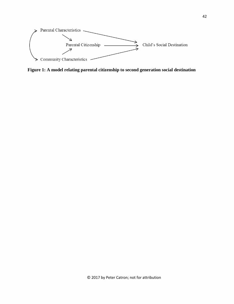
42


Figure 1: A model relating parental citizenship to second generation social destination

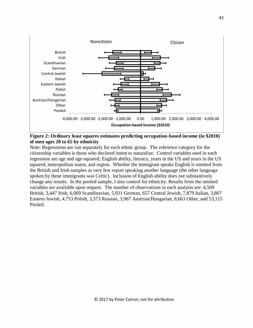
43


Figure 2: Ordinary least squares estimates predicting occupation-based income (in $2010) of men ages 20 to 65 by ethnicity Note: Regressions are run separately for each ethnic group. The reference category for the citizenship variables is those who declared intent to naturalize. Control variables used in each regression are age and age-squared, English ability, literacy, years in the US and years in the US squared, metropolitan status, and region. Whether the immigrant speaks English is omitted from the British and Irish samples as very few report speaking another language (the other language spoken by these immigrants was Celtic). Inclusion of English ability does not substantively change any results. In the pooled sample, I also control for ethnicity. Results from the omitted variables are available upon request. The number of observations in each analysis are: 4,569 British, 3,447 Irish, 6,069 Scandinavian, 5,931 German, 657 Central Jewish, 7,879 Italian, 3,807 Eastern Jewish, 4,753 Polish, 3,373 Russian, 3,967 Austrian/Hungarian, 8,663 Other, and 53,115 Pooled.

-4,000.00 -3,000.00 -2,000.00 -1,000.00 0.00 1,000.00 2,000.00 3,000.00 4,000.00

Pooled

Other

Austrian/Hungarian

Russian

Polish

Eastern Jewish

Italian

Central Jewish

German

Scandinavian

Irish

British

Occupation-based Income ($2010)

Noncitizen Citizen

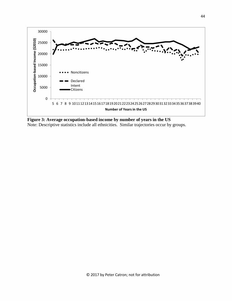
44


Figure 3: Average occupation-based income by number of years in the US Note: Descriptive statistics include all ethnicities. Similar trajectories occur by groups.

0

5000

10000

15000

20000

25000

30000

5 6 7 8 9 10111213141516171819202122232425262728293031323334353637383940

Occ

up

ati

on

-ba

sed

In

com

e (

$2

01

0)

Number of Years in the US

Noncitizens

Declared

IntentCitizens

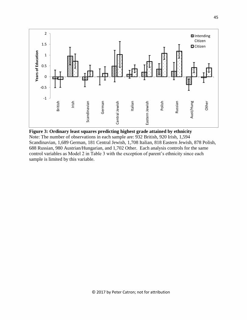
45


Figure 3: Ordinary least squares predicting highest grade attained by ethnicity Note: The number of observations in each sample are: 932 British, 920 Irish, 1,594 Scandinavian, 1,689 German, 181 Central Jewish, 1,708 Italian, 818 Eastern Jewish, 878 Polish, 688 Russian, 980 Austrian/Hungarian, and 1,702 Other. Each analysis controls for the same control variables as Model 2 in Table 3 with the exception of parent’s ethnicity since each sample is limited by this variable.

-1

-0.5

0

0.5

1

1.5

2

Bri

tish

Iris

h

Sca

nd

ina

via

n

Ge

rma

n

Ce

ntr

al

Jew

ish

Ita

lia

n

Ea

ste

rn J

ew

ish

Po

lish

Ru

ssia

n

Au

st/H

un

g

Oth

er

Ye

ars

of

Ed

uca

tio

n

Intending

Citizen

Citizen

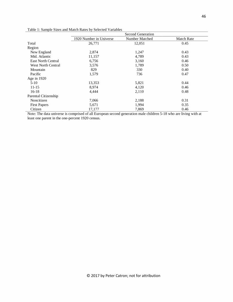
46


Table 1: Sample Sizes and Match Rates by Selected Variables Second Generation 1920 Number in Universe Number Matched Match Rate Total 26,771 12,051 0.45 Region New England 2,874 1,247 0.43 Mid. Atlantic 11,157 4,789 0.43 East North Central 6,756 3,160 0.46 West North Central 3,576 1,789 0.50 Mountain 829 330 0.40 Pacific 1,579 736 0.47 Age in 1920 5-10 13,353 5,821 0.44 11-15 8,974 4,120 0.46 16-18 4,444 2,110 0.48 Parental Citizenship Noncitizen 7,066 2,188 0.31 First Papers 5,671 1,994 0.35 Citizen 17,177 7,869 0.46 Note: The data universe is comprised of all European second generation male children 5-18 who are living with at least one parent in the one-percent 1920 census.

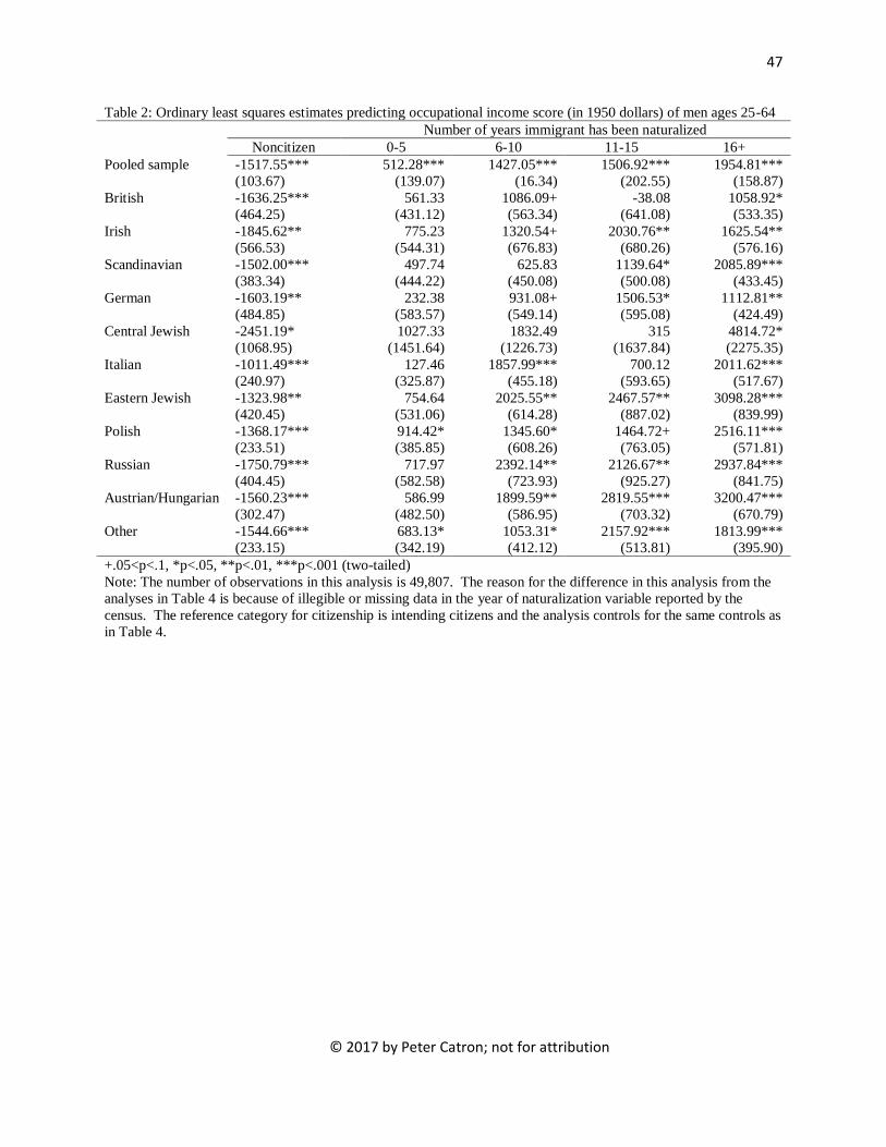
47


Table 2: Ordinary least squares estimates predicting occupational income score (in 1950 dollars) of men ages 25-64 Number of years immigrant has been naturalized Noncitizen 0-5 6-10 11-15 16+ Pooled sample -1517.55***

(103.67) 512.28***

(139.07) 1427.05***

(16.34) 1506.92***

(202.55) 1954.81***

(158.87) British -1636.25***

(464.25) 561.33

(431.12) 1086.09+ (563.34)

-38.08 (641.08)

1058.92* (533.35)

Irish -1845.62** (566.53)

775.23 (544.31)

1320.54+ (676.83)

2030.76** (680.26)

1625.54** (576.16)

Scandinavian -1502.00*** (383.34)

497.74 (444.22)

625.83 (450.08)

1139.64* (500.08)

2085.89*** (433.45)

German -1603.19** (484.85)

232.38 (583.57)

931.08+ (549.14)

1506.53* (595.08)

1112.81** (424.49)

Central Jewish -2451.19* (1068.95)

1027.33 (1451.64)

1832.49 (1226.73)

315 (1637.84)

4814.72* (2275.35)

Italian -1011.49*** (240.97)

127.46 (325.87)

1857.99*** (455.18)

700.12 (593.65)

2011.62*** (517.67)

Eastern Jewish -1323.98** (420.45)

754.64 (531.06)

2025.55** (614.28)

2467.57** (887.02)

3098.28*** (839.99)

Polish -1368.17*** (233.51)

914.42* (385.85)

1345.60* (608.26)

1464.72+ (763.05)

2516.11*** (571.81)

Russian -1750.79*** (404.45)

717.97 (582.58)

2392.14** (723.93)

2126.67** (925.27)

2937.84*** (841.75)

Austrian/Hungarian -1560.23*** (302.47)

586.99 (482.50)

1899.59** (586.95)

2819.55*** (703.32)

3200.47*** (670.79)

Other -1544.66*** (233.15)

683.13* (342.19)

1053.31* (412.12)

2157.92*** (513.81)

1813.99*** (395.90)

+.05<p<.1, *p<.05, **p<.01, ***p<.001 (two-tailed) Note: The number of observations in this analysis is 49,807. The reason for the difference in this analysis from the analyses in Table 4 is because of illegible or missing data in the year of naturalization variable reported by the census. The reference category for citizenship is intending citizens and the analysis controls for the same controls as in Table 4.

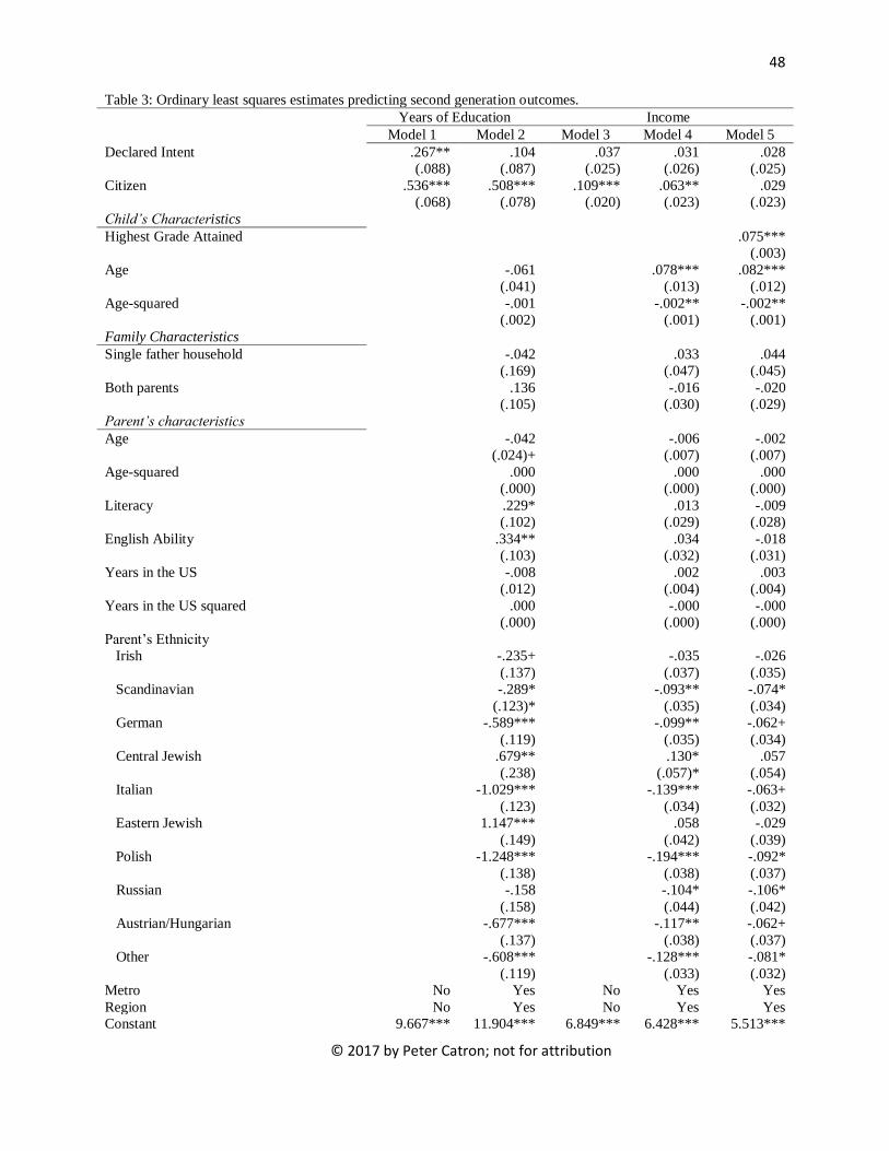
48


Table 3: Ordinary least squares estimates predicting second generation outcomes. Years of Education Income Model 1 Model 2 Model 3 Model 4 Model 5 Declared Intent .267**

(.088) .104

(.087) .037

(.025) .031

(.026) .028

(.025) Citizen .536***

(.068) .508***

(.078) .109***

(.020) .063** (.023)

.029 (.023)

Child’s Characteristics Highest Grade Attained .075***

(.003) Age -.061

(.041) .078***

(.013) .082***

(.012) Age-squared -.001

(.002) -.002**

(.001) -.002**

(.001) Family Characteristics Single father household -.042

(.169) .033

(.047) .044

(.045) Both parents .136

(.105) -.016

(.030) -.020

(.029) Parent’s characteristics Age -.042

(.024)+ -.006

(.007) -.002

(.007) Age-squared .000

(.000) .000

(.000) .000

(.000) Literacy .229*

(.102) .013

(.029) -.009

(.028) English Ability .334**

(.103) .034

(.032) -.018

(.031) Years in the US -.008

(.012) .002

(.004) .003

(.004) Years in the US squared .000

(.000) -.000

(.000) -.000

(.000) Parent’s Ethnicity Irish -.235+

(.137) -.035

(.037) -.026

(.035) Scandinavian -.289*

(.123)* -.093**

(.035) -.074* (.034)

German -.589*** (.119)

-.099** (.035)

-.062+ (.034)

Central Jewish .679** (.238)

.130* (.057)*

.057 (.054)

Italian -1.029*** (.123)

-.139*** (.034)

-.063+ (.032)

Eastern Jewish 1.147*** (.149)

.058 (.042)

-.029 (.039)

Polish -1.248*** (.138)

-.194*** (.038)

-.092* (.037)

Russian -.158 (.158)

-.104* (.044)

-.106* (.042)

Austrian/Hungarian -.677*** (.137)

-.117** (.038)

-.062+ (.037)

Other -.608*** (.119)

-.128*** (.033)

-.081* (.032)

Metro No Yes No Yes Yes Region No Yes No Yes Yes Constant 9.667*** 11.904*** 6.849*** 6.428*** 5.513***

49


(.059) (.571) (.017) (.167) (.164) N 12,051 12,051 9,483 9,483 9,362 R-squared .01 .08 .04 .07 .142 +.05<p<.1, *p<.05, **p<.01, ***p<.001 (two-tailed)

50


Table 4: Timing of parental citizenship predicting educational attainment Model 1 Citizenship timing (before son born ref) Parent Naturalized When Child was 0-5 -.043

(.098) Parent Naturalized When Child was 6-12 .019

(.132) Parent Naturalized When Child was a Teenager (13-18) -.605*

(.303) Observations 7,878 +.05<p<.1, *p<.05, **p<.01, ***p<.001 (two-tailed) Note: models control for the same control variables as in Model 2 of Table 3.

Immigrant Socioeconomic Attainment across Generations in

Documents