Image Segmentation CIS 601 Fall 2004 Longin Jan Latecki.

Image Segmentation

CIS 601 Fall 2004

Longin Jan Latecki

Image Segmentation

• Segmentation divides an image into its constituent regions or objects.

• Segmentation of images is a difficult task in image processing. Still under research.

• Segmentation allows to extract objects in images.

• Segmentation is unsupervised learning.

• Model based object extraction, e.g., template matching, is supervised learning.

What it is useful for

• After a successful segmenting the image, the contours of objects can be extracted using edge detection and/or border following techniques.

• Shape of objects can be described.• Based on shape, texture, and color objects can be

identified.• Image segmentation techniques are extensively used in

similarity searches, e.g.:

http://elib.cs.berkeley.edu/photos/blobworld/

Segmentation Algorithms

• Segmentation algorithms are based on one of two basic properties of color, gray values, or texture: discontinuity and similarity.

• First category is to partition an image based on abrupt changes in intensity, such as edges in an image.

• Second category are based on partitioning an image into regions that are similar according to a predefined criteria. Histogram thresholding approach falls under this category.

Domain spaces

spatial domain (row-column (rc) space)

histogram spaces

color space

texture space

other complex feature space

Clustering in Color Space

1. Each image point is mapped to a point in a color space, e.g.:

Color(i, j) = (R (i, j), G(i, j), B(i, j))

It is many to one mapping.

2. The points in the color space are grouped to clusters.

3. The clusters are then mapped back to regions in the image.

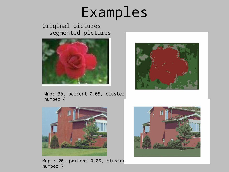
Examples

Mnp: 30, percent 0.05, cluster number 4

Mnp : 20, percent 0.05, cluster number 7

Original pictures segmented pictures

Displaying objects in the Segmented Image

• The objects can be distinguished by assigning an arbitrary pixel value or average pixel value to the pixels belonging to the same clusters.

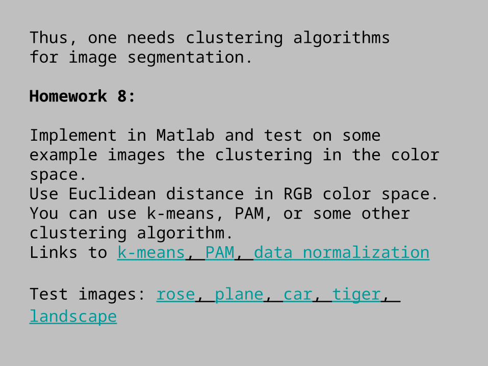
Thus, one needs clustering algorithms for image segmentation.

Homework 8:

Implement in Matlab and test on some example images the clustering in the color space. Use Euclidean distance in RGB color space.You can use k-means, PAM, or some other clustering algorithm.Links to k-means, PAM, data normalization

Test images: rose, plane, car, tiger, landscape

Segmentation by Thresholding

• Suppose that the gray-level histogram corresponds to an image f(x,y) composed of dark objects on the light background, in such a way that object and background pixels have gray levels grouped into two dominant modes. One obvious way to extract the objects from the background is to select a threshold ‘T’ that separates these modes.

• Then any point (x,y) for which f(x,y) < T is called an object point, otherwise, the point is called a background point.

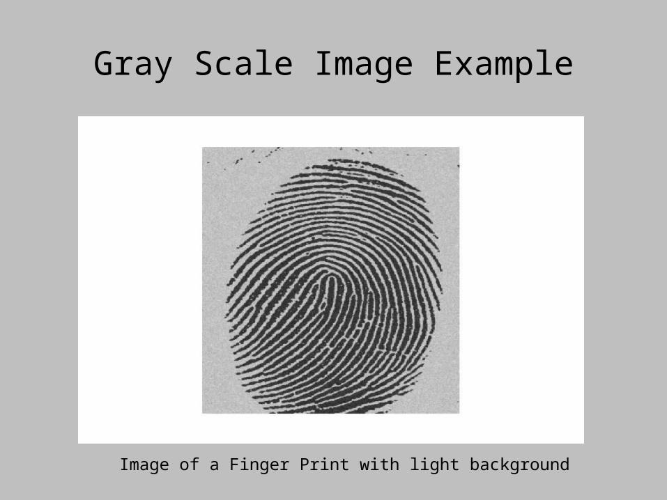
Gray Scale Image Example

Image of a Finger Print with light background

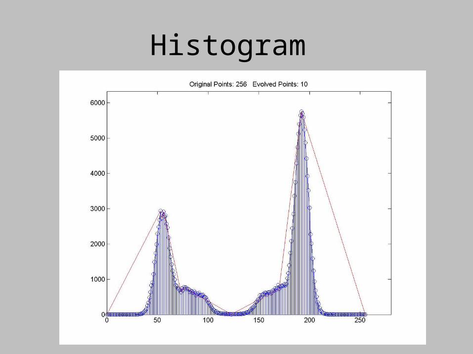
Histogram

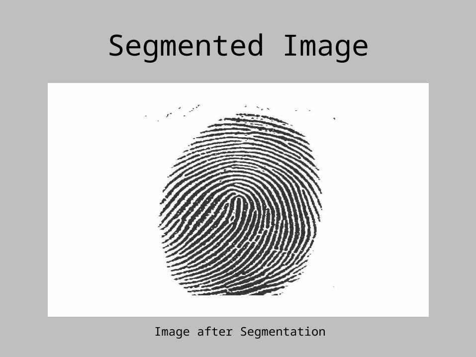
Segmented Image

Image after Segmentation

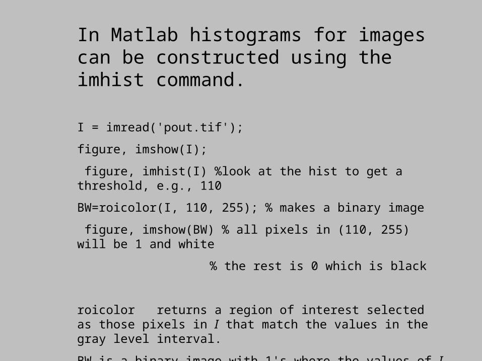
In Matlab histograms for images can be In Matlab histograms for images can be constructed using the imhist command.constructed using the imhist command.

I = imread('pout.tif');

figure, imshow(I);

figure, imhist(I) %look at the hist to get a threshold, e.g., 110

BW=roicolor(I, 110, 255); % makes a binary image

figure, imshow(BW) % all pixels in (110, 255) will be 1 and white

% the rest is 0 which is black

roicolor returns a region of interest selected as those pixels in I that match the values in the gray level interval.

BW is a binary image with 1's where the values of I match the values of the interval.

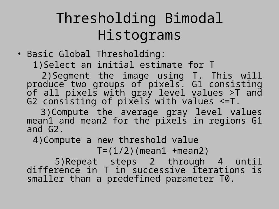
Thresholding Bimodal Histograms

• Basic Global Thresholding: 1)Select an initial estimate for T 2)Segment the image using T. This will produce two

groups of pixels. G1 consisting of all pixels with gray level values >T and G2 consisting of pixels with values <=T.

3)Compute the average gray level values mean1 and mean2 for the pixels in regions G1 and G2.

4)Compute a new threshold value T=(1/2)(mean1 +mean2) 5)Repeat steps 2 through 4 until difference in T in

successive iterations is smaller than a predefined parameter T0.

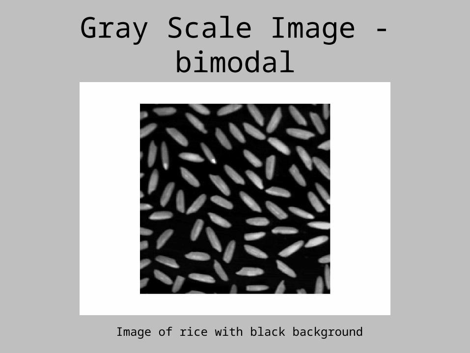
Gray Scale Image - bimodal

Image of rice with black background

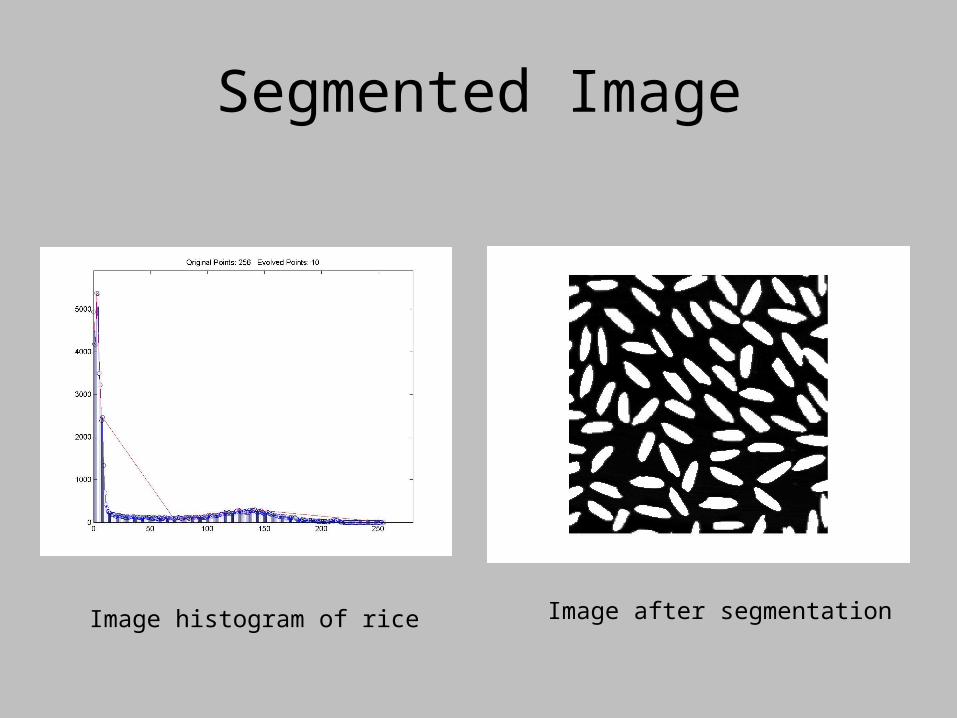
Segmented Image

Image after segmentationImage histogram of rice

Basic Adaptive Thresholding:

Images having uneven illumination makes it difficult to segment using histogram, this approach is to divide the original image into sub images and use the thresholding process to each of the sub images.

Multimodal Histogram

• If there are three or more dominant modes in the image histogram, the histogram has to be partitioned by multiple thresholds.

• Multilevel thresholding classifies a point (x,y) as belonging to one object class

if T1 < (x,y) <= T2, to the other object class if f(x,y) > T2 and to the background if f(x,y) <= T1.

Thresholding multimodal histograms

• A method based on

Discrete Curve Evolution

to find thresholds in the histogram.

• The histogram is treated as a polylineand is simplified until a few vertices remain.

• Thresholds are determined by vertices that are local minima.

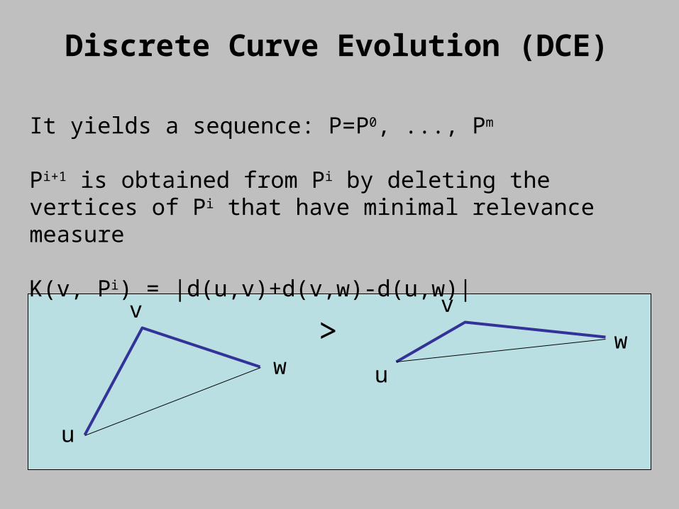
Discrete Curve Evolution (DCE)

u

v

w u

v

w

It yields a sequence: P=P0, ..., Pm

Pi+1 is obtained from Pi by deleting the vertices of Pi that have minimal relevance measure

K(v, Pi) = |d(u,v)+d(v,w)-d(u,w)|

>

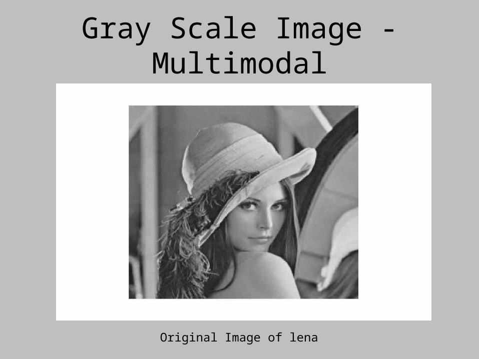
Gray Scale Image - Multimodal

Original Image of lena

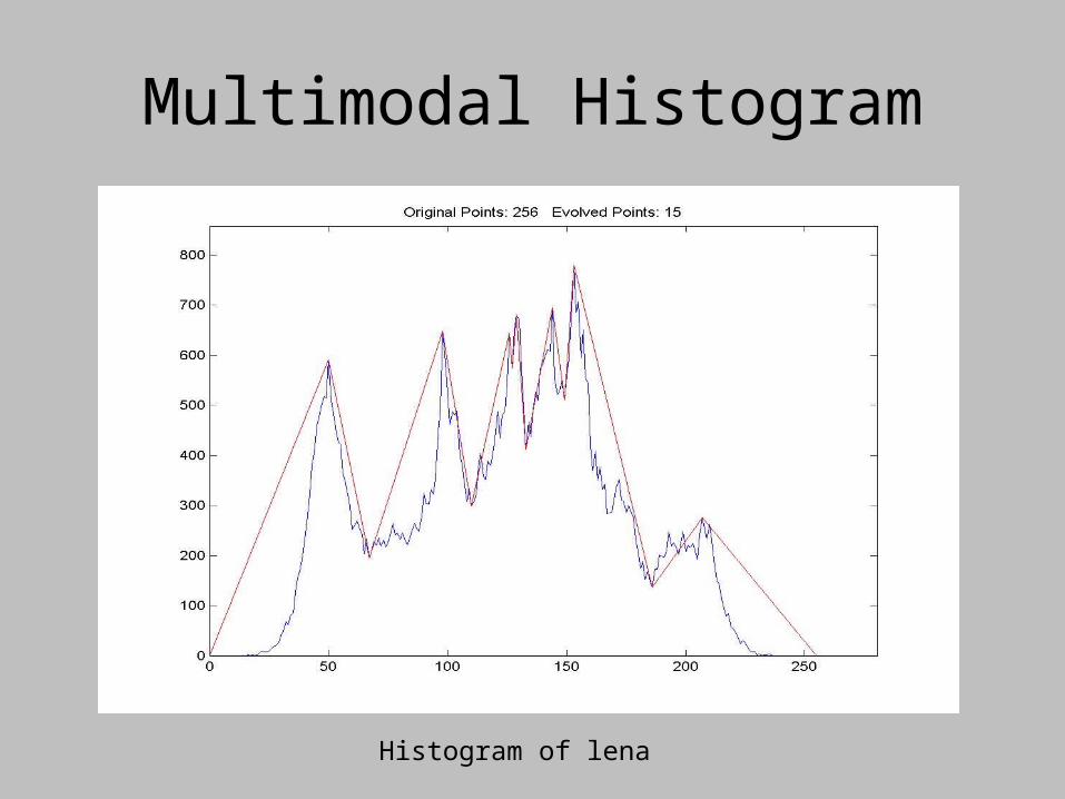
Multimodal Histogram

Histogram of lena

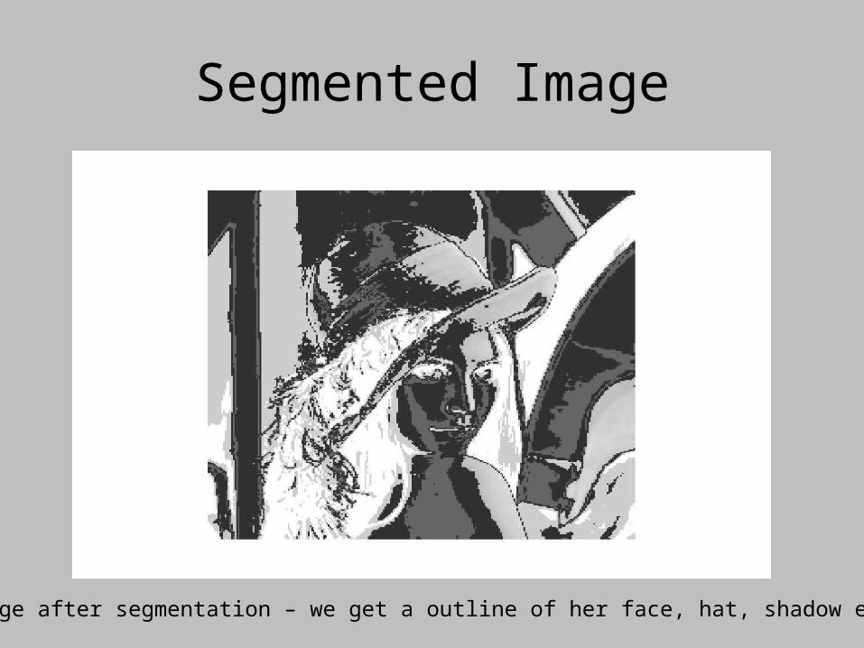
Segmented Image

Image after segmentation – we get a outline of her face, hat, shadow etc

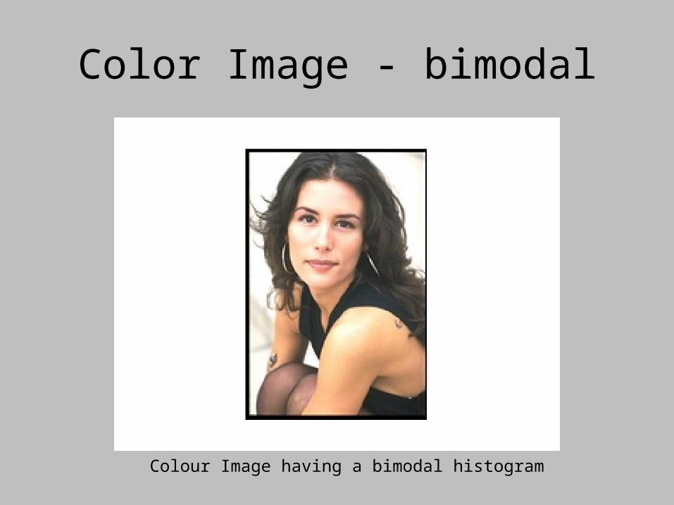
Color Image - bimodal

Colour Image having a bimodal histogram

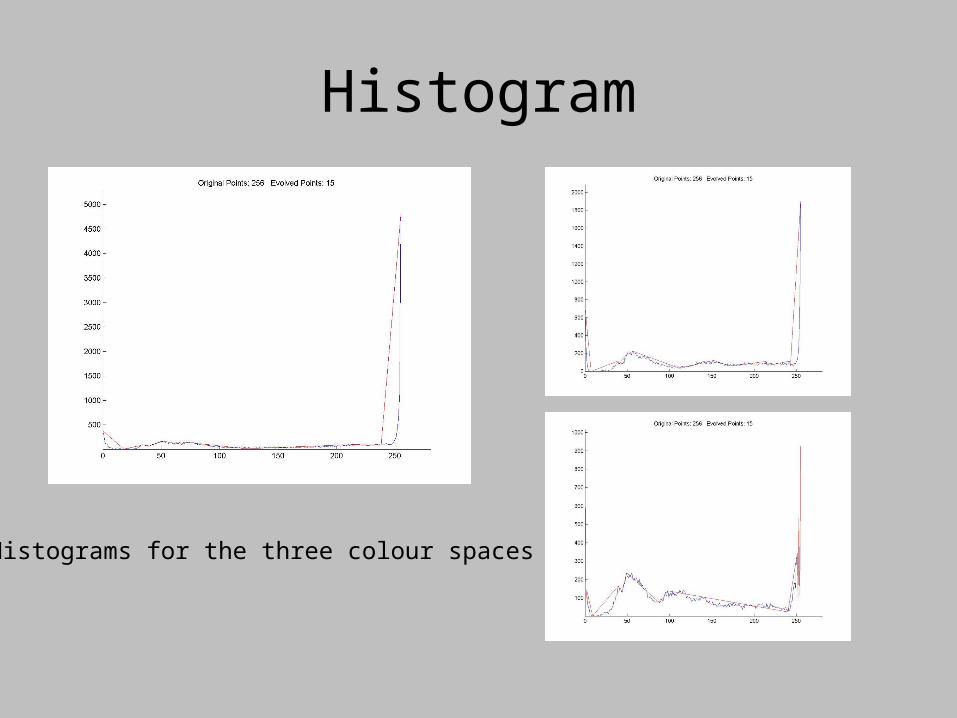
Histogram

Histograms for the three colour spaces

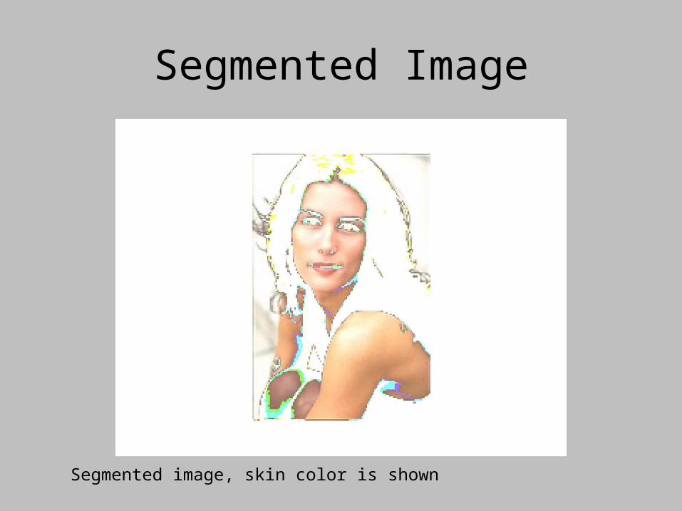
Segmented Image

Segmented image, skin color is shown

Split and Merge

• The goal of Image Segmentation is to find regions that represent objects or meaningful parts of objects. Major problems of image segmentation are result of noise in the image. 

• An image domain X must be segmented in N different regions R(1),…,R(N)

• The segmentation rule is a logical predicate of the form P(R)

Introduction

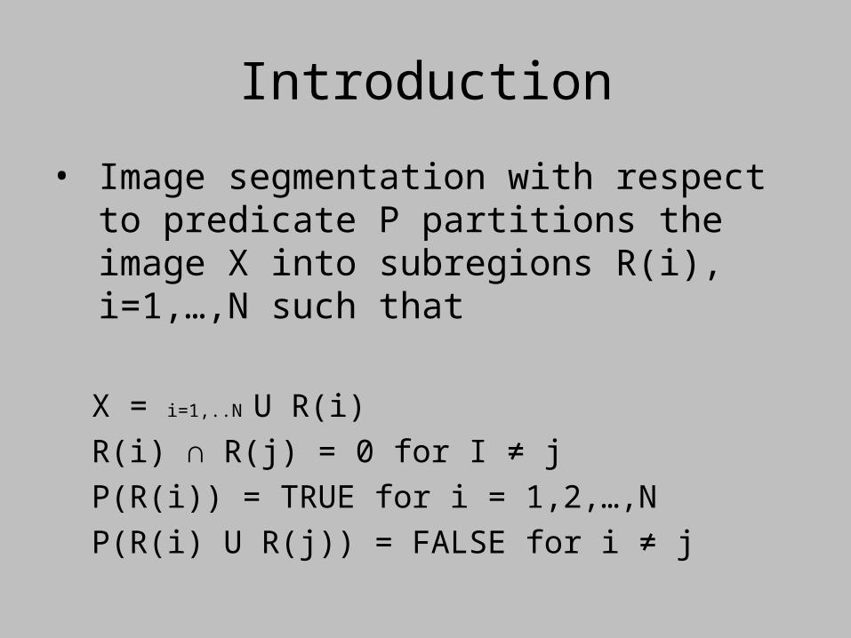
• Image segmentation with respect to predicate P partitions the image X into subregions R(i), i=1,…,N such that

X = i=1,..N U R(i)

R(i) ∩ R(j) = 0 for I ≠ j

P(R(i)) = TRUE for i = 1,2,…,N

P(R(i) U R(j)) = FALSE for i ≠ j

Introduction

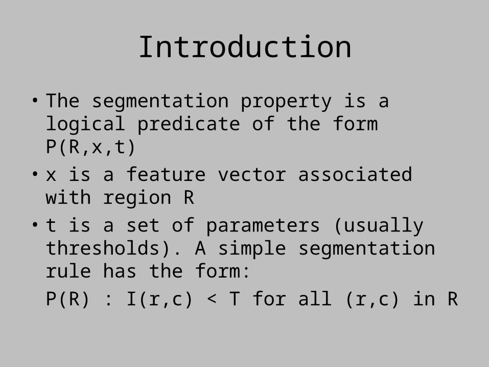
• The segmentation property is a logical predicate of the form P(R,x,t)

• x is a feature vector associated with region R

• t is a set of parameters (usually thresholds). A simple segmentation rule has the form:

P(R) : I(r,c) < T for all (r,c) in R

Introduction

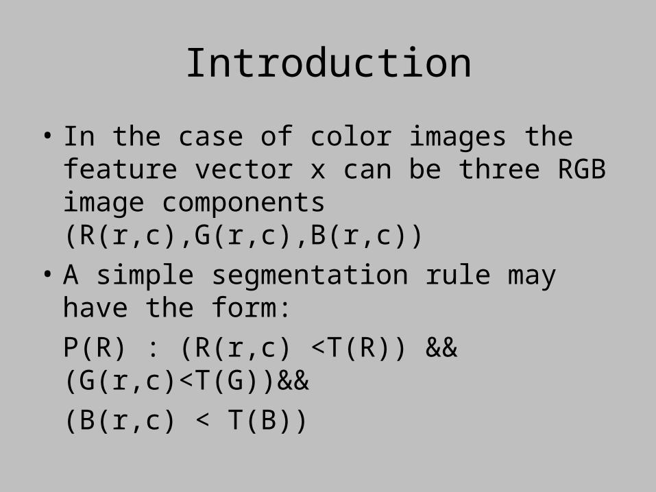
• In the case of color images the feature vector x can be three RGB image components (R(r,c),G(r,c),B(r,c))

• A simple segmentation rule may have the form:

P(R) : (R(r,c) <T(R)) && (G(r,c)<T(G))&&

(B(r,c) < T(B))

Region Growing (Merge)

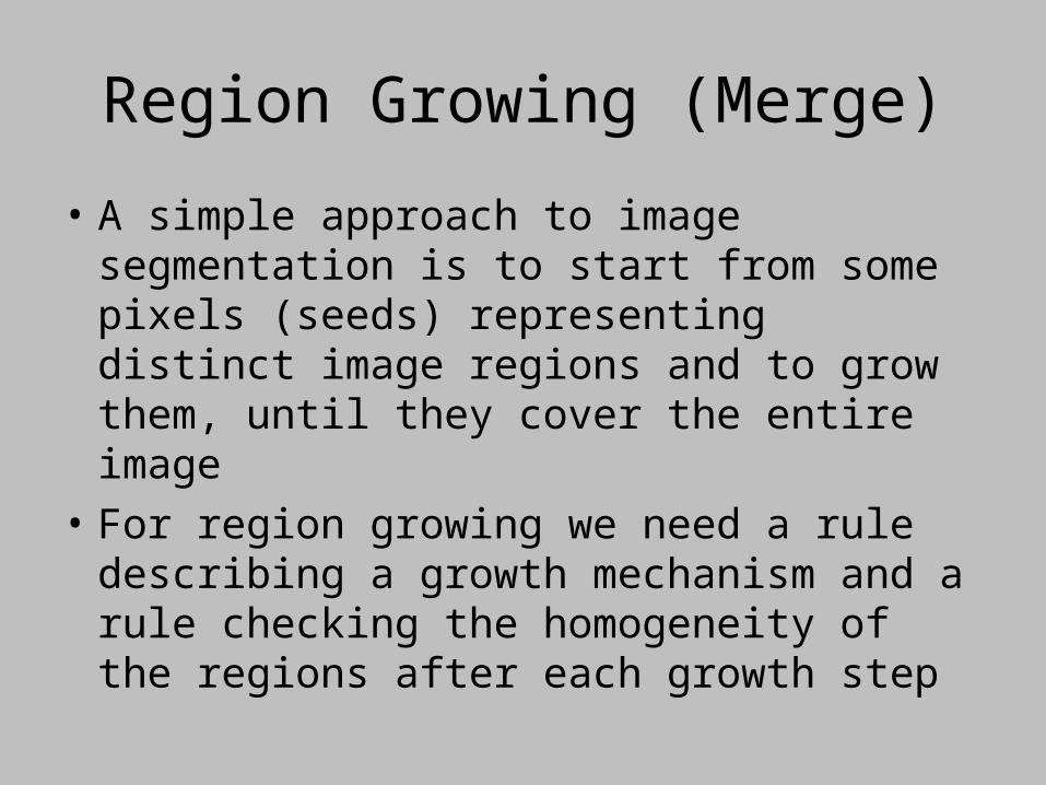
• A simple approach to image segmentation is to start from some pixels (seeds) representing distinct image regions and to grow them, until they cover the entire image

• For region growing we need a rule describing a growth mechanism and a rule checking the homogeneity of the regions after each growth step

Region Growing

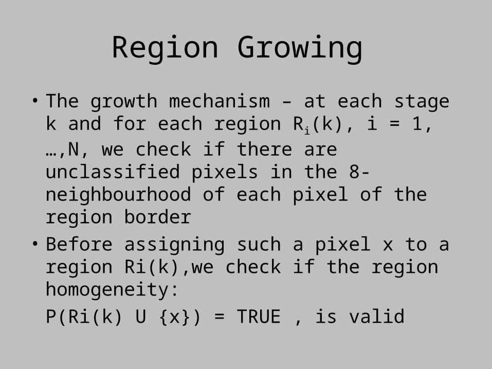
• The growth mechanism – at each stage k and for each region Ri(k), i = 1,…,N, we check if there are unclassified pixels in the 8-neighbourhood of each pixel of the region border

• Before assigning such a pixel x to a region Ri(k),we check if the region homogeneity:

P(Ri(k) U {x}) = TRUE , is valid

Region Growing Predicate

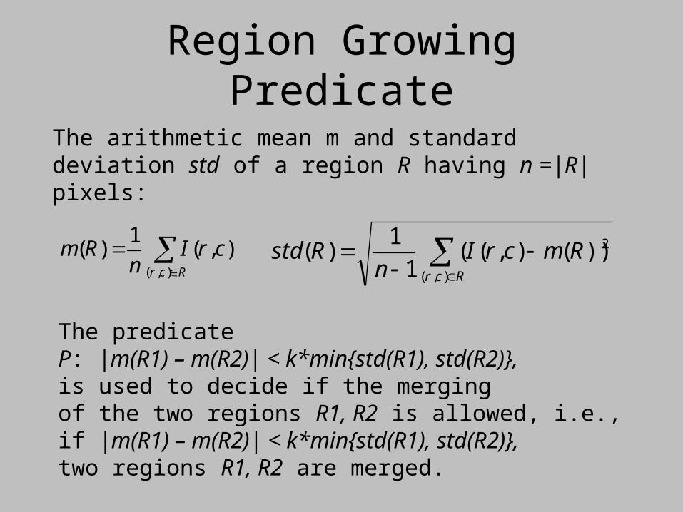
The predicate P: |m(R1) – m(R2)| < k*min{std(R1), std(R2)}, is used to decide if the mergingof the two regions R1, R2 is allowed, i.e.,if |m(R1) – m(R2)| < k*min{std(R1), std(R2)}, two regions R1, R2 are merged.

Rcr

crIn

Rm),(

),(1

)(

The arithmetic mean m and standard deviation std of a region R having n =|R| pixels:

Rcr

RmcrIn

Rstd),(

2))(),((1

1)(

Split

• The opposite approach to region growing is region splitting.

• It is a top-down approach and it starts with the assumption that the entire image is homogeneous

• If this is not true, the image is split into four sub images

• This splitting procedure is repeated recursively until we split the image into homogeneous regions

Split

• If the original image is square N x N, having dimensions that are powers of 2(N = 2n):

• All regions produced but the splitting algorithm are squares having dimensions M x M , where M is a power of 2 as well.

• Since the procedure is recursive, it produces an image representation that can be described by a tree whose nodes have four sons each

• Such a tree is called a Quadtree.

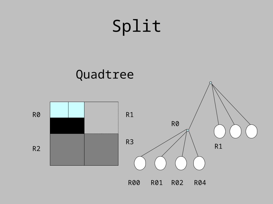
Split

Quadtree

R0 R1

R2R3

R0

R1

R00 R01 R02 R04

Split

• Splitting techniques disadvantage, they create regions that may be adjacent and homogeneous, but not merged.

• Split and Merge method is an iterative algorithm that includes both splitting and merging at each iteration:

Split / Merge

• If a region R is inhomogeneous (P(R)= False) then is split into four sub regions

• If two adjacent regions Ri,Rj are homogeneous (P(Ri U Rj) = TRUE), they are merged

• The algorithm stops when no further splitting or merging is possible

Split / Merge

• The split and merge algorithm produces more compact regions than the pure splitting algorithm

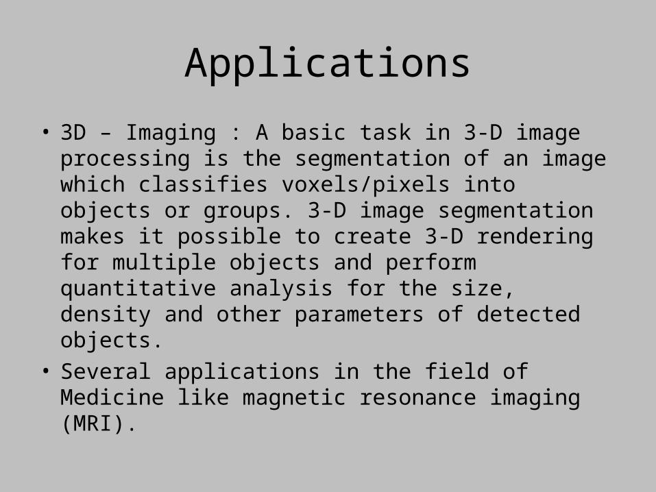
Applications

• 3D – Imaging : A basic task in 3-D image processing is the segmentation of an image which classifies voxels/pixels into objects or groups. 3-D image segmentation makes it possible to create 3-D rendering for multiple objects and perform quantitative analysis for the size, density and other parameters of detected objects.

• Several applications in the field of Medicine like magnetic resonance imaging (MRI).

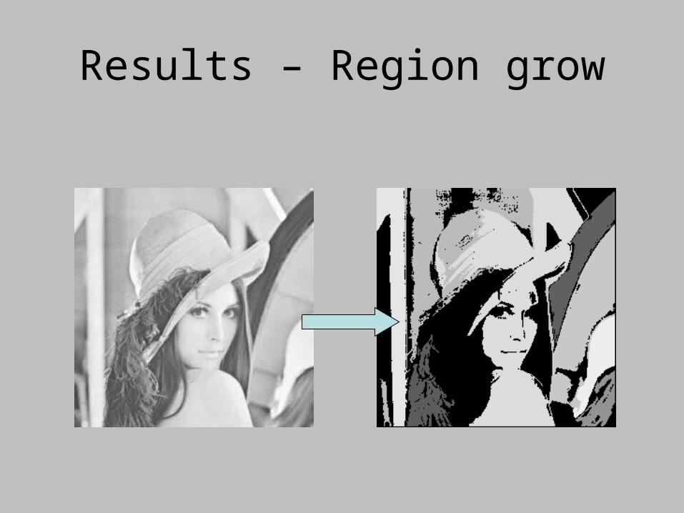
Results – Region grow

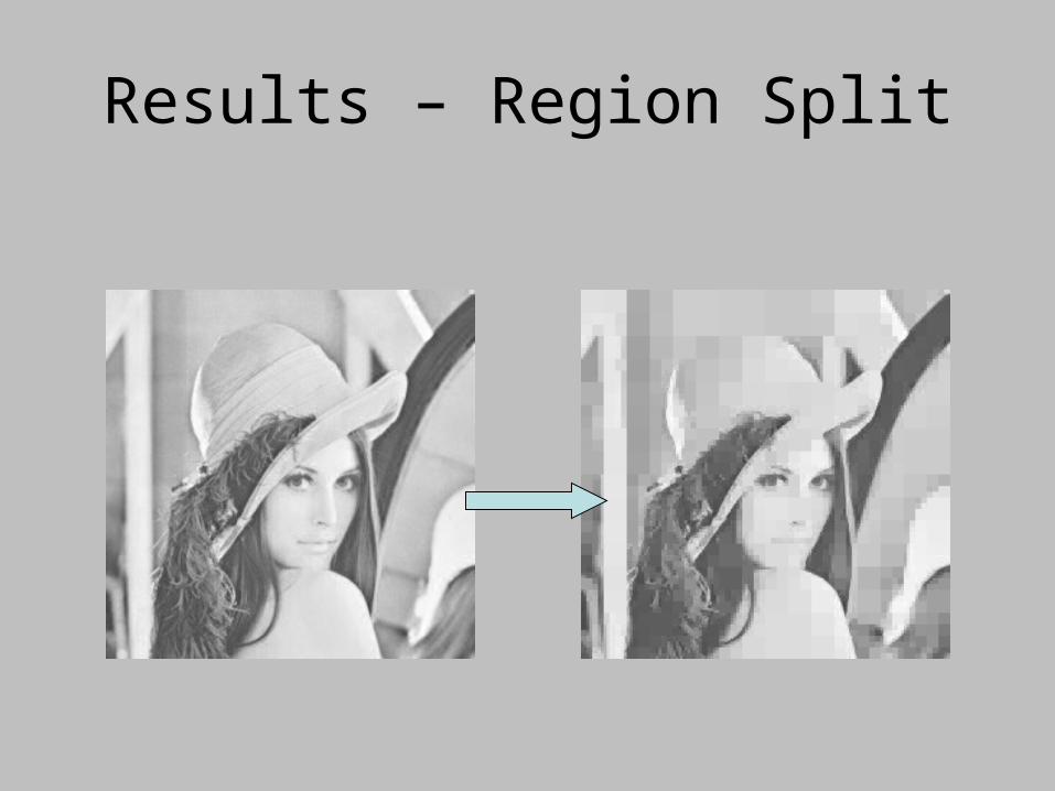
Results – Region Split

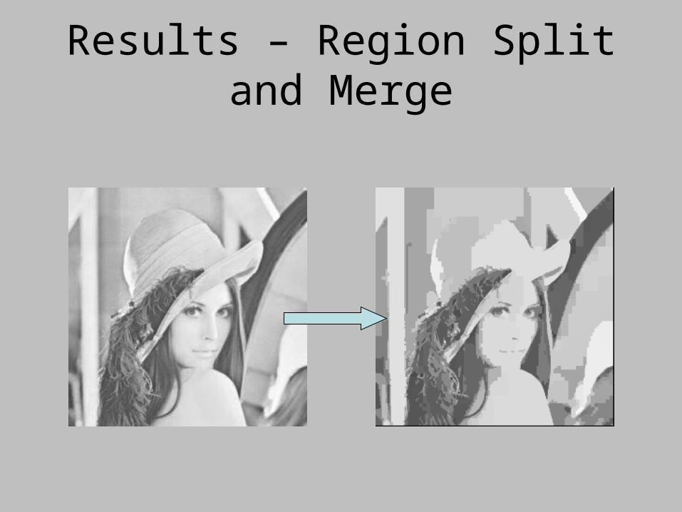
Results – Region Split and Merge