Pattern Recognition, Vol. 23, No. 9, pp. 961-973, 1990 Printed in Great Britain 0031-3203/90 $3.00 ~- .00 Pergamon Press pie ~) 1990 Pattern Recognition Society IMAGE SEGMENTATION BY A PARALLEL, NON- PARAMETRIC HISTOGRAM BASED CLUSTERING ALGORITHM* ALIREZA KHOTANZAD and ABDELMAJID BOUARFA Image Processing and Analysis Laboratory, Electrical Engineering Department, Southern Methodist University, Dallas, Texas 75275, U.S.A. (Received 21 July 1989; received for publication 29 January 1990) Abstract--This paper describes a totally automatic non-parametric clustering algorithm and its appli- cation to unsupervised image segmentation, The clusters are found by mode analysis of the multi- dimensional histogram of the considered vectors through a non-iterative peak-climbing approach. Systematic methods for automatic selection of an appropriate histogram cell size are developed and discussed. The algorithm is easily parallelizable and is simulated on a SEQUENT parallel computer. Image segmentation is performed by clustering features extracted from small local areas of the image. Segmentation of textured, color, and gray-level images are considered. Eight-dimensional random field model based features, three-dimensional RGB components, and one-dimensional gray levels are utilized for these three types of images respectively. For texture segmentation, an image plane cluster validity procedure based on region growing of the mapped back clusters in the feature space is developed. Most of the phases are also parallelized resulting in almost linear speed ups. Quite satisfactory results are obtained in all cases. Image segmentation Texture segmentation Color segmentation Cluster analysis Multi-dimensional histogram Segmentation by clustering Non-parametric clustering Parallel processing 1. INTRODUCTION Image segmentation is one of the first tasks to be performed in an image analysis system. It involves partitioning the image into connected regions each of which is uniform in some property such as gray level, color, texture, etc. Accurate segmentation is a critical component in the operation of the system since errors in this stage propagate to later phases. There are a wide variety of image segmentation techniques as surveyed in references (1,2). Feature space clustering is one of the most popular of these methods. C31 Typically, several characteristic features are extracted from small local areas of the image. Each class of homogeneous regions is assumed to form a distinct cluster in the space of these features. Consequently, a clustering method is used to group the points in the feature space into clusters. These clusters are then mapped back to the original spatial domain to produce a segmentation of the image. In a general segmentation task, very little a priori knowledge about the underlying structure of the extracted feature data from the image is available. Information such as the number of uniform regions in the image (corresponding to the number of clusters in the feature space) and the form of probability density of features are not known. Thus, truly non- parametric clustering techniques need to be utilized. * Supported in part by DARPA Grant MDA-903-86-C- 0182. The literature on cluster analysis is both vol- uminous and diverse, t4.5) provide excellent surveys of the existing techniques. Major limitations of these schemes are: (1) requiring the specification of some a priori knowledge about the structure of the data or other parameters which control the clustering process, (2) slowness due to extensive computations required, especially in the case of iterative methods, (3) bias toward particular cluster shapes (e.g. spheri- cal, hyperellipsoidal, etc.). This study involves dev- elopment of a totally non-parametric and automatic clustering algorithm which overcomes the drawbacks listed above. Our main motivation is to apply this algorithm to the image segmentation problem. Interfacing the two raises other issues such as cluster validity in the image plane which are also addressed in this study. However, it should be noted that the application is by no means restricted to image seg- mentation and the algorithm is general enough to be applied to a wide variety of other clustering prob- lems. The proposed algorithm is based upon the meth- odology described by Narendra and Goldberg. ~61 It involves analysing the multi-dimensional histogram of the feature vectors rather than working with the vectors themselves, The histogram summarizes the distribution of feature vectors and approximates the probability density of the data. Each significant peak (mode) in the histogram is taken as a distinct cluster. The boundaries between clusters correspond to the local minima or valleys that surround each peak. 961

Welcome message from author
This document is posted to help you gain knowledge. Please leave a comment to let me know what you think about it! Share it to your friends and learn new things together.
Transcript
Pattern Recognition, Vol. 23, No. 9, pp. 961-973, 1990 Printed in Great Britain
0031-3203/90 $3.00 ~- .00 Pergamon Press pie
~) 1990 Pattern Recognition Society
IMAGE SEGMENTATION BY A PARALLEL, NON- PARAMETRIC HISTOGRAM BASED CLUSTERING
ALGORITHM*
ALIREZA KHOTANZAD and ABDELMAJID BOUARFA Image Processing and Analysis Laboratory, Electrical Engineering Department, Southern Methodist
University, Dallas, Texas 75275, U.S.A.
(Received 21 July 1989; received for publication 29 January 1990)
Abstract--This paper describes a totally automatic non-parametric clustering algorithm and its appli- cation to unsupervised image segmentation, The clusters are found by mode analysis of the multi- dimensional histogram of the considered vectors through a non-iterative peak-climbing approach. Systematic methods for automatic selection of an appropriate histogram cell size are developed and discussed. The algorithm is easily parallelizable and is simulated on a SEQUENT parallel computer. Image segmentation is performed by clustering features extracted from small local areas of the image. Segmentation of textured, color, and gray-level images are considered. Eight-dimensional random field model based features, three-dimensional RGB components, and one-dimensional gray levels are utilized for these three types of images respectively. For texture segmentation, an image plane cluster validity procedure based on region growing of the mapped back clusters in the feature space is developed. Most of the phases are also parallelized resulting in almost linear speed ups. Quite satisfactory results are obtained in all cases.
Image segmentation Texture segmentation Color segmentation Cluster analysis Multi-dimensional histogram Segmentation by clustering Non-parametric clustering Parallel processing
1. I N T R O D U C T I O N
Image segmentation is one of the first tasks to be performed in an image analysis system. It involves partitioning the image into connected regions each of which is uniform in some property such as gray level, color, texture, etc. Accurate segmentation is a critical component in the operation of the system since errors in this stage propagate to later phases. There are a wide variety of image segmentation techniques as surveyed in references (1,2). Feature space clustering is one of the most popular of these methods. C31 Typically, several characteristic features are extracted from small local areas of the image. Each class of homogeneous regions is assumed to form a distinct cluster in the space of these features. Consequently, a clustering method is used to group the points in the feature space into clusters. These clusters are then mapped back to the original spatial domain to produce a segmentation of the image.
In a general segmentation task, very little a priori knowledge about the underlying structure of the extracted feature data from the image is available. Information such as the number of uniform regions in the image (corresponding to the number of clusters in the feature space) and the form of probability density of features are not known. Thus, truly non- parametric clustering techniques need to be utilized.
* Supported in part by DARPA Grant MDA-903-86-C- 0182.
The literature on cluster analysis is both vol- uminous and diverse, t4.5) provide excellent surveys of the existing techniques. Major limitations of these schemes are: (1) requiring the specification of some a priori knowledge about the structure of the data or other parameters which control the clustering process, (2) slowness due to extensive computations required, especially in the case of iterative methods, (3) bias toward particular cluster shapes (e.g. spheri- cal, hyperellipsoidal, etc.). This study involves dev- elopment of a totally non-parametric and automatic clustering algorithm which overcomes the drawbacks listed above. Our main motivation is to apply this algorithm to the image segmentation problem. Interfacing the two raises other issues such as cluster validity in the image plane which are also addressed in this study. However, it should be noted that the application is by no means restricted to image seg- mentation and the algorithm is general enough to be applied to a wide variety of other clustering prob- lems.
The proposed algorithm is based upon the meth- odology described by Narendra and Goldberg. ~61 It involves analysing the multi-dimensional histogram of the feature vectors rather than working with the vectors themselves, The histogram summarizes the distribution of feature vectors and approximates the probability density of the data. Each significant peak (mode) in the histogram is taken as a distinct cluster. The boundaries between clusters correspond to the local minima or valleys that surround each peak.
961
962 ALIREZA KHOTANZAD and ABDELMAJID BOUARFA
Thus, one need not know the number of clusters in advance as the method determines it automatically. Furthermore, being a non-iterative procedure and working with the histogram instead of the data are two factors which significantly reduce the required computation time.
Although the idea of identifying clusters in multi- dimensional data by mode analysis using histograms has been studied before, ~6"7) none of the previously developed algorithms were completely automatic. For instance, automatic selection of an appropriate histogram cell size which is an important parameter is not addressed. In this study we propose systematic methods for this task. In addition, the application to image segmentation brings about the requirement of interaction and feedback between the output of the clustering algorithm and its resulting segmentation in the image plane. Peaks detected in the feature space do not necessarily correspond to distinct regions in the image. As such spatial domain cluster validity tests are developed to correct such problems. Finally, the parallel structure of the selected approach which was another motivation for its selec- tion, is exploited to speed up the execution. Both the clustering and segmentation procedures are implemented on a SEQUENT parallel computer resulting in nearly linear speed-ups.
The general approach presented here can be applied to segmentation of a wide variety of imagery. The only difference will be in the attributes (fea- tures) used to represent each type. In this study, segmentation of textured, color, and gray level images are considered. However, the emphasis is on the more complex problem of texture segmentation where intensity edge detection techniques com- pletely fail. This is so because they cannot distinguish between texture edges (boundaries between homo- geneously textured regions) and microedges (inten- sity variations within a uniform texture). Textural features used in this study are the estimated par- ameters of random field models fitted to the local region under consideration. Their good performance in other classification and segmentation studies ~s'9'l°) motivated their utilization. In case of color images, the three color components, R, G, and B associated with a pixel are used as features. Similarly, pixel intensity is the utilized feature for gray level image segmentation.
2. HISTOGRAM GENERATION IN THE MULTIDIMENSIONAL SPACE
The first step toward the generation of the his- togram is the quantization of the L-dimensional fea- ture space into non-overlapping cells. As a result, each cell will encompass a certain number of data points (feature vectors) and the histogram is gen- erated by counting the number of vectors falling into each cell. Since the dynamic range of the vectors in each dimension can be quite different, the cell size
fm~(2: C(1.4)
cO,a)
C(L2)
c(1,1) fmin(2)
fmin(1)
C(2.4) C(3,4) C(4,4)
c(2,a) c(a,3) c(4.3)
c(2.2) c(~,2) c(4.2)
c(2.1) c(3,1) c(4.1)
fmax(l)
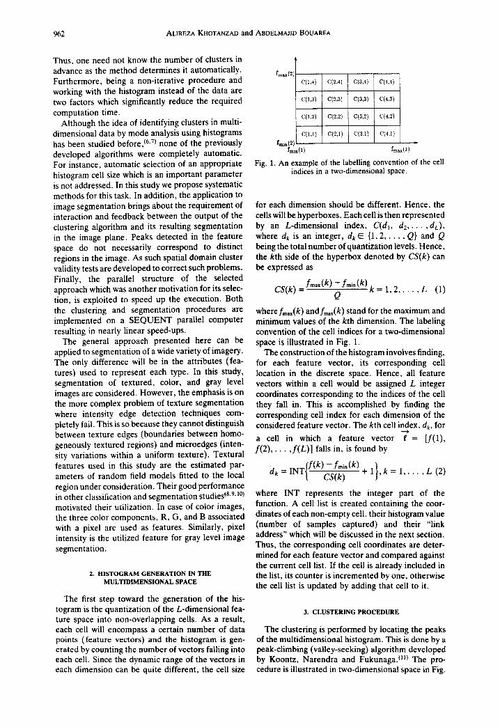
Fig. 1. An example of the labelling convention of the cell indices in a two-dimensional space.
for each dimension should be different. Hence, the cells will be hyperboxes. Each cell is then represented by an L-dimensional index, C(dl, d2 . . . . . dL), where dk is an integer, dk ~ {1, 2 . . . . . Q} and Q being the total number of quantization levels. Hence, the kth side of the hyperbox denoted by CS(k) can be expressed as
f~ax(k) - f m i . ( k ) CS(k) = k = 1, 2 . . . . . L (1) Q
where fmax(k) and fmin(k) stand for the maximum and minimum values of the kth dimension. The labeling convention of the cell indices for a two-dimensional space is illustrated in Fig. 1.
The construction of the histogram involves finding, for each feature vector, its corresponding cell location in the discrete space. Hence, all feature vectors within a cell would be assigned L integer coordinates corresponding to the indices of the cell they fall in. This is accomplished by finding the corresponding cell index for each dimension of the considered feature vector. The kth cell index, dk, for
.....}
a cell in which a feature vector f = [f(1), f(2) . . . . . f (L) ] falls in, is found by
(f(k) (k) 1},k 1, , L ( 2 ) dk = INT / ~ + . . . .
where INT represents the integer part of the function. A cell list is created containing the coor- dinates of each non-empty cell, their histogram value (number of samples captured) and their "link address" which will be discussed in the next section. Thus, the corresponding cell coordinates are deter- mined for each feature vector and compared against the current cell list. If the cell is already included in the list, its counter is incremented by one, otherwise the cell list is updated by adding that cell to it.
3. CLUSTERING PROCEDURE
The clustering is performed by locating the peaks of the multidimensional histogram. This is done by a peak-climbing (valley-seeking) algorithm developed by Koontz, Narendra and FukunagaJ m The pro- cedure is illustrated in two-dimensional space in Fig.
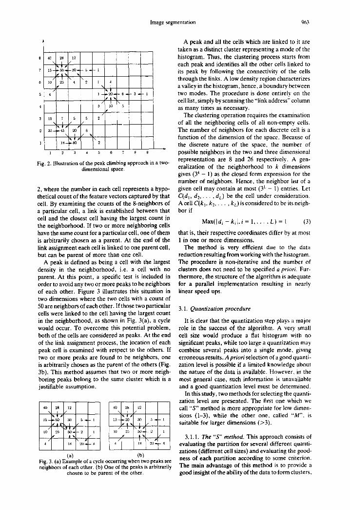
Image segmentation 963
40 28 12
\ ~ ~I /
1 5 - ~ 5 0 ~ - - 3 0 ~ - 5 . ~ - 1
I0 / 25 4
/ 4
15 7 5 5
35 ~ ~ 45 20 8
1 8 - - , . 8 0
1 4
\ 1 1 - - b 2 0 ~ - - 8 . 9 - - 3 ~ - 1
4 / I x
3 I0 5 d
/
2
\
2
1 2 3 4 5 6 7 8 9
Fig. 2. Illustration of the peak climbing approach in a two- dimensional space.
2, where the number in each cell represents a hypo- thetical count of the feature vectors captured by that cell. By examining the counts of the 8-neighbors of a particular cell, a link is established between that cell and the closest cell having the largest count in the neighborhood. If two or more neighboring cells have the same count for a particular celt, one of them is arbitrarily chosen as a parent. At the end of the link assignment each cell is linked to one parent cell, but can be parent of more than one cell.
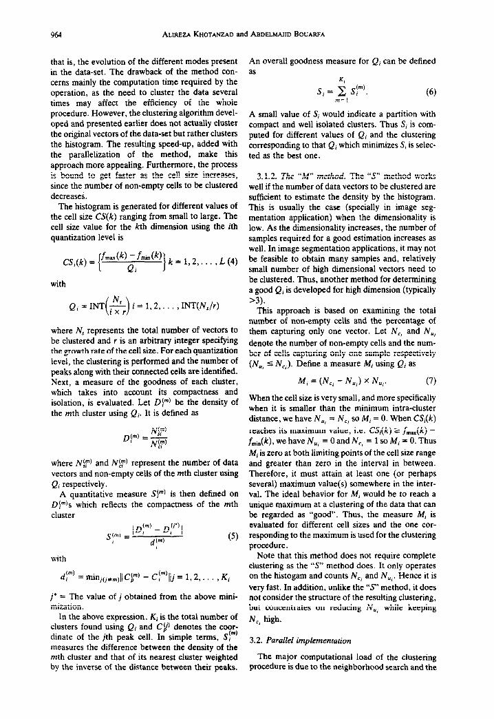
A peak is defined as being a cell with the largest density in the neighborhood, i.e. a cell with no parent. At this point, a specific test is included in order to avoid any two or more peaks to be neighbors of each other. Figure 3 illustrates this situation in two dimensions where the two cells with a count of 50 are neighbors of each other. If those two particular cells were linked to the cell having the largest count in the neighborhood, as shown in Fig. 3(a), a cycle would occur. To overcome this potential problem, both of the cells are considered as peaks. At the end of the link assignment process, the location of each peak cell is examined with respect to the others. If two or more peaks are found to be neighbors, one is arbitrarily chosen as the parent of the others (Fig. 3b). This method assumes that two or more neigh- boring peaks belong to the same cluster which is a justifiable assumption.
40 28 12 40 28 12
1 5 - - b 5 0 30 5 ~ - 1 15- -~ . .50 30 5 - - - 1
/ 21 / " , t p 10 95 ~ 2 1 10 25 , 50 . - '2 1
" I ~ / " I " / / \ # / \ P 4 18 _'20 ~ - - 8 4 18 2 0 - r - 8
(a) (b) Fig. 3. (a) Example of a cycle occurring when two peaks are neighbors of each other. (b) One of the peaks is arbitrarily
chosen to be parent of the other.
A peak and all the cells which are linked to it are taken as a distinct cluster representing a mode of the histogram. Thus, the clustering process starts from each peak and identifies all the other cells linked to its peak by following the connectivity of the cells through the links. A low density region characterizes a valley in the histogram, hence, a boundary between two modes. The procedure is done entirely on the cell list, simply by scanning the "link address" column as many times as necessary.
The clustering operation requires the examination of all the neighboring cells of all non-empty cells. The number of neighbors for each discrete cell is a function of the dimension of the space. Because of the discrete nature of the space, the number of possible neighbors in the two and three dimensional representation are 8 and 26 respectively. A gen- eralization of the neighborhood to k dimensions gives (3 k - 1) as the closed form expression for the number of neighbors. Hence, the neighbor list of a given cell may contain at most (3 L - 1) entries. Let C(dl, d2 . . . . . dL) be the cell under consideration. A cell C(kl, k2 . . . . . kL) is considered to be its neigh- bor if
Max(Id i - k i l , i = 1 . . . . . L) = 1 (3)
that is, their respective coordinates differ by at most 1 in one or more dimensions.
The method is very efficient due to the data reduction resulting from working with the histogram. The procedure is non-iterative and the number of clusters does not need to be specified a priori. Fur- thermore, the structure of the algorithm is adequate for a parallel implementation resulting in nearly linear speed ups.
3.1. Quantization procedure
It is clear that the quantization step plays a major role in the success of the algorithm. A very small cell size would produce a fiat histogram with no significant peaks, while too large a quantization may combine several peaks into a single mode. giving erroneous results. A priori selection of a good quanti- zation level is possible if a limited knowledge about the nature of the data is available. However, in the most general case, such information is unavailable and a good quantization level must be determined.
In this study, two methods for selecting the quanti- zation level are presented. The first one which we call "S" method is more appropriate for low dimen- sions (1-3), while the other one, called "M". is suitable for larger dimensions (>3).
3.1.1. The "S" method. This approach consists of evaluating the partition for several different quanti- zations (different cell sizes) and evaluating the good- ness of each partition according to some criterion. The main advantage of this method is to provide a good insight of the ability of the data to form clusters,
964 ALIREZA KHOTANZAD and ABDELUAJID BOUARFA
that is, the evolution of the different modes present in the data-set. The drawback of the method con- cerns mainly the computation time required by the operation, as the need to cluster the data several times may affect the efficiency of the whole procedure. However, the clustering algorithm devel- oped and presented earlier does not actually cluster the original vectors of the data-set but rather clusters the histogram. The resulting speed-up, added with the parallelization of the method, make this approach more appealing. Furthermore, the process is bound to get faster as the cell size increases, since the number of non-empty cells to be clustered decreases.
The histogram is generated for different values of the cell size CS(k) ranging from small to large. The cell size value for the kth dimension using the ith quantization level is
CS;(k) = [~m”(k)Qj~m~(k)] k = 1,2,. . . , L (4)
with
Qi = IbJT(s) i = 1,2,. . . , INT(N,/r)
where N, represents the total number of vectors to be clustered and r is an arbitrary integer specifying the growth rate of the cell size. For each quantization level, the clustering is performed and the number of peaks along with their connected cells are identified. Next, a measure of the goodness of each cluster, which takes into account its compactness and isolation, is evaluated. Let 0:“) be the density of the mth cluster using Qi. It is defined as
where N$“) and N$“) represent the number of data vectors and non-empty cells of the mth cluster using Qi respectively.
A quantitative measure Sjm) is then defined on DIm)s which reflects the compactness of the mth cluster
(5)
with
dj”’ = minj(j+mjl(Cbm) - Cy’Ilj = 1,2,. . . , Ki
‘* I = The value of j obtained from the above mini- mization .
In the above expression, Ki is the total number of clusters found using Qi and C$jl denotes the coor- dinate of the jth peak cell. In simple terms, SF’ measures the difference between the density of the mth cluster and that of its nearest cluster weighted by the inverse of the distance between their peaks.
An overall goodness measure for Qi can be defined as
4
Si = z Sl”‘. (6) m=l
A small value of S; would indicate a partition with compact and well isolated clusters. Thus Si is com- puted for different values of Qj and the clustering corresponding to that Qi which minimizes S; is selec- ted as the best one.
3.1.2. The “M” method. The “S” method works well if the number of data vectors to be clustered are sufficient to estimate the density by the histogram. This is usually the case (specially in image seg- mentation application) when the dimensionality is low. As the dimensionality increases, the number of samples required for a good estimation increases as well. In image segmentation applications, it may not be feasible to obtain many samples and, relatively small number of high dimensional vectors need to be clustered. Thus, another method for determining a good Qi is developed for high dimension (typically >3).
This approach is based on examining the total number of non-empty cells and the percentage of them capturing only one vector. Let N,, and N,,
denote the number of non-empty cells and the num- ber of cells capturing only one sample respectively (NMi 4 Nci). Define a measure Mi using Q; as
Mi = (N,, - N”i) X N”~. (7)
When the cell size is very small, and more specifically when it is smaller than the minimum intra-cluster distance, we have N,, = Nci SO Mi = 0. When CSi(k)
reaches its maximum value, i.e. CSi(k) 2 f,,,&k) - fmin(k), we have NUi = 0 and Nci = 1 SO Mi = 0. Thus
Mi is zero at both limiting points of the cell size range and greater than zero in the interval in between. Therefore, it must attain at least one (or perhaps several) maximum value(s) somewhere in the inter- val. The ideal behavior for Mi would be to reach a unique maximum at a clustering of the data that can be regarded as “good”. Thus, the measure Mi is evaluated for different cell sizes and the one cor- responding to the maximum is used for the clustering procedure.
Note that this method does not require complete clustering as the “s” method does. It only operates on the histogam and counts N,, and N,, . Hence it is
very fast. In addition, unlike the “s” method, it does not consider the structure of the resulting clustering, but concentrates on reducing N,, while keeping
N,, high.
3.2. Parallel implementation
The major computational load of the clustering procedure is due to the neighborhood search and the
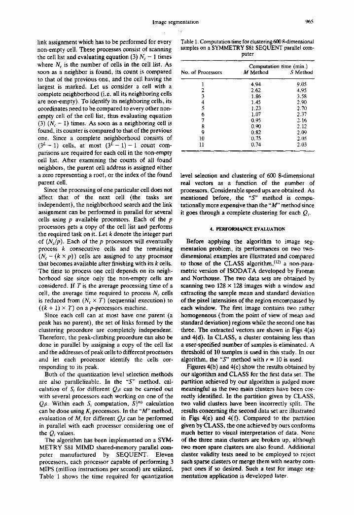
Image segmentation
link assignment which has to be performed for every non-empty cell. These processes consist of scanning the cell list and evaluating equation (3) Nc - 1 times where Nc is the number of cells in the cell list. As soon as a neighbor is found, its count is compared to that of the previous one, and the cell having the largest is marked. Let us consider a cell with a complete neighborhood (i.e. all its neighboring cells are non-empty). To identify its neighboring cells, its coordinates need to be compared to every other non- empty cell of the cell list, thus evaluating equation (3) (No - 1) times. As soon as a neighboring cell is found, its counter is compared to that of the previous one. Since a complete neighborhood consists of (3 L - 1) cells, at most (3 L - 1 ) - 1 count com- parisons are required for each cell in the non-empty cell list. After examining the counts of all found neighbors, the parent cell address is assigned either a zero representing a root, or the index of the found parent cell.
Since the processing of one particular cell does not affect that of the next cell (the tasks are independent), the neighborhood search and the link assignment can be performed in parallel for several cells using p available processors. Each of the p processors gets a copy of the cell list and performs the required task on it. Let k denote the integer part of (N~/p). Each of the p processors will eventually process k consecutive cells and the remaining (No - (k × p)) cells are assigned to any processor that becomes available after finishing with its k cells. The time to process one cell depends on its neigh- borhood size since only the non-empty cells are considered. If T is the average processing time of a cell, the average time required to process Nc cells is reduced from (N~ × T) (sequential execution) to ((k + 1) × T) on a p-processors machine.
Since each cell can at most have one parent (a peak has no parent), the set of links formed by the clustering procedure are completely independent. Therefore, the peak-climbing procedure can also be done in parallel by assigning a copy of the cell list and the addresses of peak cells to different processors and let each processor identify the cells cor- responding to its peak.
Both of the quantization level selection methods are also parallelizable. In the "S" method, cal- culation of Si for different Q~ can be carried out with several processors each working on one of the Q~. Within each Si computation, S~ ") calculation can be done using Ki processors. In the "M" method, evaluation of Mi for different Q~ can be performed in parallel with each processor considering one of the Qi values.
The algorithm has been implemented on a SYM- METRY $81 MIMD shared-memory parallel com- puter manufactured by SEQUENT. Eleven processors, each processor capable of performing 3 MIPS (million instructions per second) are utilized. Table 1 shows the time required for quantization
965
Table 1. Computation time for clustering 600 8-dimensional samples on a SYMMETRY $81 SEQUENT parallel com-
puter
Computation time (rain.) No. of Processors M Method S Method
1 4.94 9.05 2 2.62 4.95 3 1.86 3.58 4 1.45 2.90 5 1.23 2.70 6 1.07 2.37 7 0.95 2.16 8 0.90 2.12 9 0.82 2.09
10 0.75 2.05 11 0.74 2.03
level selection and clustering of 600 8-dimensional real vectors as a function of the number of processors. Considerable speed ups are obtained. As mentioned before, the "S" method is compu- tationaUy more expensive than the "M" method since it goes through a complete clustering for each Qi.
4. PERFORMANCE EVALUATION
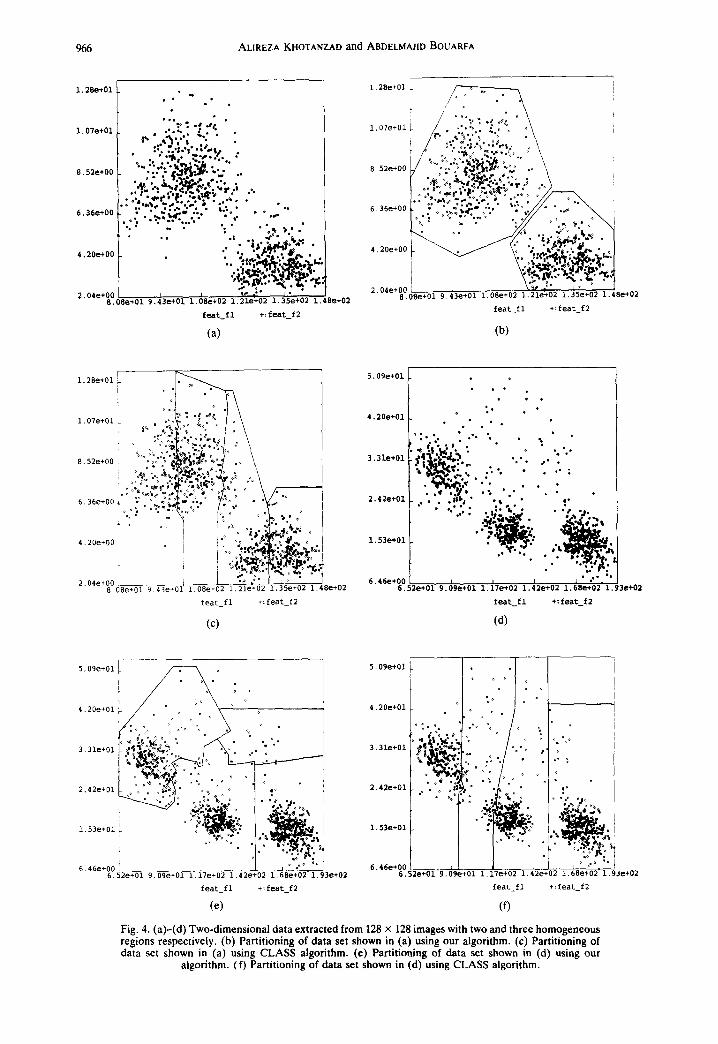
Before applying the algorithm to image seg- mentation problem, its performances on two two- dimensional examples are illustrated and compared to those of the CLASS algorithm, 02) a non-para- metric version of ISODATA developed by Fromm and Northouse. The two data sets are obtained by scanning two 128 x 128 images with a window and extracting the sample mean and standard deviation of the pixel intensities of the region encompassed by each window. The first image contains two rather homogeneous (from the point of view of mean and standard deviation) regions while the second one has three. The extracted vectors are shown in Figs 4(a) and 4(d). In CLASS, a cluster containing less than a user-specified number of samples is eliminated. A threshold of 10 samples is used in this study. In our algorithm, the "S" method with r = 10 is used.
Figures 4(b) and 4(c) show the results obtained by our algorithm and CLASS for the first data set. The partition achieved by our algorithm is judged more meaningful as the two main clusters have been cor- rectly identified. In the partition given by CLASS, two valid clusters have been incorrectly split. The results concerning the second data set are illustrated in Figs 4(e) and 4(f). Compared to the partition given by CLASS, the one achieved by ours conforms much better to visual interpretation of data. None of the three main clusters are broken up, although two more spare clusters are also found. Additional cluster validity tests need to be employed to reject such sparse clusters or merge them with nearby com- pact ones if so desired. Such a test for image seg- mentation application is developed later.
9 6 6 A L I R E Z A KHOTANZAD a n d A B D E L M A J I D B O U A R F A
[
1.28e+01 ~ . •
• "'~" ; "# ~4 1.07e+Ol , .'.~ • ~. ,% .." "; :' "~," ~:f'.'... :
1 '-..'.'-%~':J#_ • " • : . . - {~..-. . . 8.52e+0O
. . . • | ¢. ~.:~, ..,., . ' : ' . , ~ ¢ ~ ' . p ' . ~ L ~ ' ~ .; -"
~.3~.oo . : . ~. , . : . ;~ . - . . , . ' " . ' . ,. • • ..,. ""
"'." " . . . . . . ":" " " " ~. ' "" I .o . . . % ~ . .
2.04e+00 I t ,~e ,•° , I • 8.(}8e+01 9,43e+01 1.08e+02 1.21e+02 1.35e+02 1.48e+02
feat fl +:[eat_f2
(a)
1.28e+01 !
, /~,, .C~.~.c C - : o . \
v' o ° " ~" ")l,~'..~" " . o \
. . ' . . . ~ - : ~ . ; . ' . . ~ ~ .°. o
2 04e+O0 1 i \~e ~ ~. " • 8.08e+01 9.43e+01 1.08e+02 1.21e+02 1.35e*02 1.48e+02
feat fl *: feat_f2
(b)
i. 28e÷01 o.
i °o~o
8.52e+00 ! % ° ° : ° ; J / ' i °
6.36e+00~ o oo~,%o , ,° o~
2.04e+O0 L~[_-/_t~---~ 8.08e÷01 9.43e+01 1.08e+02 1.21e*02 1.35e+02 1.48e+02
feat fl +: feat_f2
(c)
1 5.09e+01 I " "
o o
:. 4.20e+Ol I
• °
't" -, '," " "" " ' "
, ~ ' ~ ' , •
2 .4~e+01 , . • . ~ . a • . $ ~.. "" .: " • :" %~ " " " i , " ".,
... .'. ~ ~,l
I. 53e+01 o"
• .. • . ~2 . s 1
I 6.52e+01 9.09e+Ol i. 17e+02 i. 42e+02 i. 68e+02" i. 93e*02
feat_fl ÷: feat_f2
( d )
5,09e+Ol
o o
6.46e+00 L ° o • 0~ %° , I
6 . 5 ~ ~ T ' ~ 1 .17e+02 1 . 4 2 e 02 L e S e O2 1 .93e+02
feat fl +: feat_f 2
(e)
4.20e+01 i ° a' °
3.31e+01 ° i l ~ ~ o
2.42e+01 oO ~ ~o
1.53e+01
6.46e+00 6.52e+01 909e+01
o 0 . i
. - , , , .~Eo. . • ova,.~= /
I ° °" "}.° °o't i! o"o: oi
1 . 1 7 e 02 1 . 4 2 e 02 1 .68e+02 1 .§3e+02
feat_fl *: feat_f2
(f)
Fig. 4. (a)-(d) Two-dimensional data extracted from 128 x 128 images with two and three homogeneous regions respectively. (b) Partitioning of data set shown in (a) using our algorithm• (c) Partitioning of data set shown in (a) using CLASS algorithm. (e) Partitioning of data set shown in (d) using our
algorithm. (f) Partitioning of data set shown in (d) using CLASS algorithm•
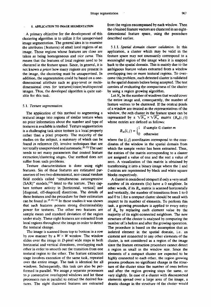
Image segmentation 967
5. APPLICATION TO IMAGE SEGMENTATION
A primary objective for the development of this clustering algorithm is to utilize it for unsupervised image segmentation. The general idea is to examine the attributes (features) of small local regions of an image. Those regions whose features are close are taken as being homogeneous and vice versa. This means that the features of local regions need to be clustered in the feature space. Since, in general, it is not known a priori how many regions are present in the image, the clustering must be unsupervised. In addition, the segmentation could be based on a one- dimensional attribute such as gray-level or multi- dimensional ones for textured/color/multispectral images. Thus, the developed algorithm is quite suit- able for this task.
5.1. Texture segmentation
The application of this method to segmenting a textural image into regions of similar texture when no prior information about the number and type of textures is available is studied. Texture segmentation is a challenging task since texture is a local property rather than a pixel property. The majority of the studies on the subject, a summary of which can be found in reference (9), involve techniques that are not totally unsupervised and automatic.(8.13) The user needs to set many parameters that control feature extraction/clustering stages. Our method does not suffer from such problems.
Texture characterization is done using eight features. Six of these features are estimated par- ameters of two two-dimensional, non-causal random field models called "simultaneous autoregressive (SAR)" models, (14) fitted to the texture. They cap- ture texture activity in [horizontal, vertical] and [diagonal, off-diagonal] directions. The details of these features and the procedure for their estimation can be found in. 19' 1o. 14) In those studies it was shown that such features possess strong discriminability power for textures. The other two features are sample mean and standard deviation of the region under study. These eight features are extracted from local regions throughout the image in order to detect the textural change.
The image is scanned from top to bottom in a row by row manner by a W x W window. The window slides over the image in D-pixel wide steps in both horizontal and vertical directions, overlapping each other in order to smooth out the transition from one textural region to the other. The feature extraction stage involves execution of the same task, repeated over the entire image. The task is identical for all windows. Subsequently, this task can also be per- formed in parallel. We assign p separate processors to p consecutive overlapped windows and let these processors run in parallel to extract the desired fea- tures. The eight discussed features are extracted
from the region encompassed by each window. Then the obtained feature vectors are clustered in an eight- dimensional feature space, using the procedure described earlier.
5.1.1. Spatial domain duster validation. In this application, a cluster which may be valid in the feature space may not necessarily correspond to a meaningful region of the image when it is mapped back to the spatial domain. This is mainly due to the ambiguous feature values extracted from a window overlapping two or more textural regions. To over- come this problem, each detected cluster is validated in the spatial domain before being accepted. The test consists of evaluating the compactness of the cluster by using a region growing algorithm.
Let Nw be the number of windows that would cover the entire image and, consequently, the number of feature vectors to be clustered. If the central pixels of a window are treated as the representatives of the window, the ruth cluster in the feature space can be represented by a ~ x ~ matrix (Bm(i,j)) whose entries are defined as follows:
1 if sample E cluster m
B , , ( i , j ) = 0 otherwise
where the (i, j) coordinates correspond to the coor- dinates of the window in the spatial domain from which the sample vector has been extracted. Thus, the entries of the matrix corresponding to a cluster are assigned a value of one and the rest a value of zero. A visualization of this matrix is obtained by transforming it into a binary image where the 1 and 0 entries are represented by black and white square blocks respectively.
A cluster is considered compact if only a very small number of its elements (ls) have a 0 neighbor. In other words, if its Bm matrix is scanned horizontally and vertically, the number of transitions from 1 to 0 and 0 to 1 for a compact cluster should be small with respect to its number of elements. To perform this task, a growing procedure is applied to every entry of Bm by replacing each element value by the majority of its eight-connected neighbors. The new structure of the cluster is analysed by comparing the number of ls before and after the growing operation. The procedure is based on the assumption that an isolated element in the spatial domain, i.e. an element not connected to any other elements of the cluster, is not considered as a region of the image since the feature extraction procedure cannot detect a region as small as the window size. Since the elements of a compact cluster are expected to be highly connected to each other, the region growing process produces no significant change in the struc- ture of the cluster since the number of ones before and after the region growing stays the same, or vary slightly. In case of a cluster with disconnected elements spread over a large area of the image, a drastic change in the structure of the cluster would
968 ALIREZA KHOTANZAD and ABDELMAJID BOUARFA
occur due to the significant reduction of the number of ones. In this study, a reduction of more than 50% of ones is taken as an indication of an invalid cluster, which is a candidate for merging. A complete dis- appearance would indicate a noisy cluster, i.e. a cluster whose elements may belong to different regions of the image. These clusters are often created by the boundaries present in the image. A cluster which is a candidate for merging is merged with a valid one having the closest centroid. All noisy clus- ters are kept together in a single cluster processed at the end. A speed up of the process is achieved by assigning each spatial cluster to a different pro- cessor and let them perform the validation task in parallel.
After the validation process, all the valid clusters are labelled with different gray level intensity and mapped in the spatial domain for display. Finally, a cleaning operation is performed by assigning the yet unlabelled pixels (i.e. those previously classified as noisy) to the label of the majority of their eight- connected neighbors.
Table 2. The window sizes and the number of quantization levels selected by the algorithm for textured images
Selected window size Selected number of Images in p i x e i s quantization levels
Fig. 5(a) 8 5 Fig. 6(a) 12 5 Fig. 6(b) 16 4 Fig. 6(c) 8 4 Fig. 6(d) 8 4
5.1.2. Window size selection. The size of the win- dow used to scan the image plays a crucial role in the success of the segmentation. Knowing the type and the resolution of the textures in the images would solve the problem but the unsupervised assumption prevents the use of such information. The procedure used in this study is to start with a small window to perform the clustering. Then, the window size is slightly increased and the process is repeated. When the same number of clusters are obtained over two
consecutive window sizes, the process stops and the segmentation is performed using the smallest of the two for better resolution. This scheme, which seems costly at first, stays within an acceptable time range, due to the efficient parallel implementation of the segmentation procedure.
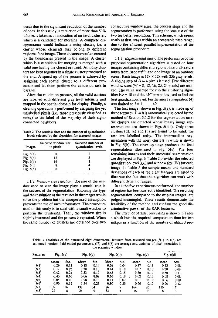
5.1.3. Experimental study. The performance of the proposed segmentation algorithm is tested on four images containing different regions of natural texture taken from Brodatz ¢15) and one image of an outdoor scene. Each image is 128 x 128 with 256 gray levels. A sliding step of D = 4 pixels is used. Five different window sizes (W = 8, 12, 16, 20, 24 pixels) are utili- zed. The value selected for r in the clustering algor- ithm is r = 10 and the "M" method is used to find the best quantization level. Furthermore i in equation (4) was limited to i = 1 , . . . , 40.
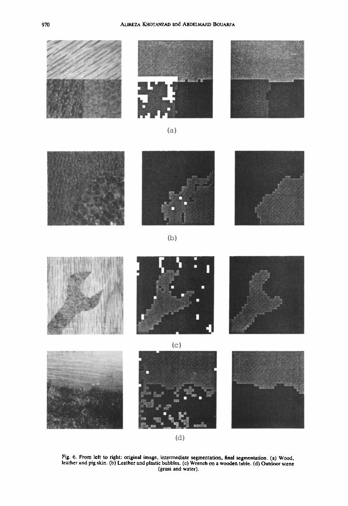
The first image, shown in Fig. 5(a), is made up of three textures. L = 8 is automatically selected by the method of Section 5.1.2 for the segmentation task. Six clusters are detected whose binary image rep- resentations are shown in Figs 5(d-i). Only three clusters (d), (e) and (h) are found to be valid, the rest are labelled noisy. The intermediate seg- mentation with the noisy clusters in white is shown in Fig. 5(b). The clean up stage produces the final segmentation illustrated in Fig. 5(c). The four remaining images and their successful segmentation are displayed in Fig. 6. Table 2 provides the selected quantization level (Qi) and window size (W) for each image. In Table 3 the sample means and standard deviations of each of the eight features are listed to illustrate the fact that the algorithm can work with different dynamic ranges.
In all the five experiments performed, the number of regions has been correctly identified. The resulting segmentation, compared to the original images, are judged meaningful. These results demonstrate the feasibility of the method and confirm the good dis- criminative power of the SAR features.
The effect of parallel processing is shown in Table 4 which lists the required computation time for two images as a function of the number of utilized pro-
Table 3. Statistics estimated random
of the extracted eight-dimensional features from textured images, f(1) to f(6) are field model parameters, f(7) and f(8) are average and variance of pixel intensities in
the scanning window
Features Fig. 5(a) Fig. 6(a) Fig. 6(b) Fig. 6(c) Fig. 6(d)
Mean Std. Mean Std. Mean Std. Mean Std. Mean f(1) 0.29 0.12 0.18 0.10 0.26 0.04 0.37 0.11 0.13 f(2) 0.12 0.12 0.30 0.10 0.14 0.10 0.07 0.10 0.20 f(3) 0.42 0.21 0.33 0.12' 0.48 0.15 0.30 0.19 0.60 f(4) 0.40 0.10 0.06 0.08 0.10 0.10 0.02 0.10 0.08 f(5) 0.05 0.10 0.28 0.13 0.11 0.07 0.01 0.10 0.06 f(6) 0.90 0.12 0.54 0.23 0.80 0.20 0.90 0.12 0.90 f(7) 132 36 138 34 86 9 164 20 116 f(8) 22 8 24 9 33 4 18 6 6
Std. 0.08 0.08 0.17 0.08 0.08 0.12
17 3
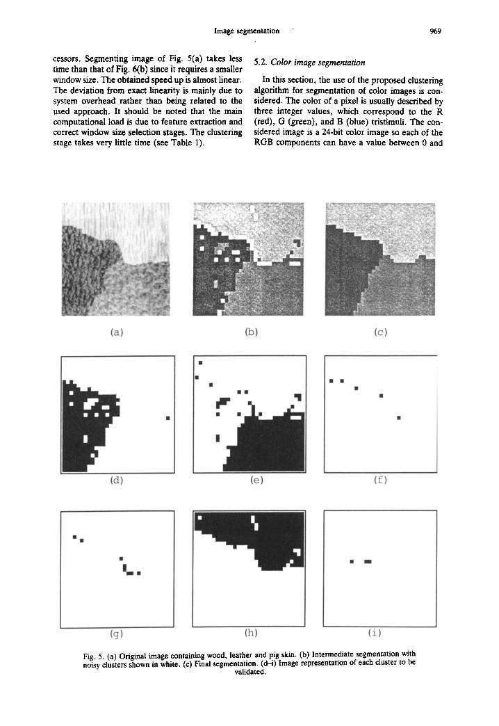
Image segmentation 969
cessors. Segmenting image of Fig. 5(a) takes less time than that of Fig. 6(b) since it requires a smaller window size. The obtained speed up is almost linear. The deviation from exact linearity is mainly due to system overhead rather than being related to the used approach. It should be noted that the main computational load is due to feature extraction and correct window size selection stages. The clustering stage takes very little time (see Table 1).
5.2. Color image segmentation
In this section, the use of the proposed clustering algorithm for segmentation of color images is con- sidered. The color of a pixel is usually described by three integer values, which correspond to the R (red), G (green), and B (blue) tristimuli. The con- sidered image is a 24-bit color image so each of the RGB components can have a value between 0 and
(a) (b) (c)
II
"I
(d) (e) (f)
• mm
(g) (h) (i)
Fig. 5. (a) Original image containing wood, leather and pig skin. (b) Intermediate segmentation with noisy clusters shown in white. (c) Final segmentation. (d-i) Image representation of each cluster to be
validated.
970 AUREZA KHOTANZAD and ABDELMAJID BOUARFA
(a)
I
(b)
(c)
I [ , % : I I
• •
N m
!
(d)
n
g
i
m
i
Fig. 6. From left to right: original image, intermediate segmentation, final segmentation. (a) Wood, leather and pig skin. (b) Leather and plastic bubbles. (c) Wrench on a wooden table. (d) Outdoor scene
(grass and water).
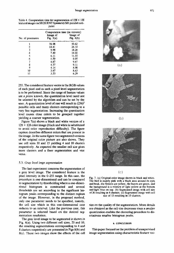
Image segmentation
Table 4. Computation time for segmentation of 128"x i~2~ ~ textural images on SEQUENT Symmetry Sgl parallel com-
puter
No. of processors
Computation time (in minutes) Image of Image of Fig. 5(a) Fig. 6(b)
1 28.08 50.62 2 14.41 26.10 3 9.98 18.20 4 7.49 14.02 5 6.11 11.55 6 5.59 9.95 7 4.87 9.67 8 4.37 9.11 9 4.14 8.90
10 3.67 8.63 11 3.53 6.29
(a)
971
255. The considered feature vector is the RGB values of each pixel and as such a pixel level segmentation is to be performed. Since the range of feature values are a priori known, the quantization level need not be selected by the algorithm and can be set by the user. A quantization level of one will result in (256) 3 possible cells and many clusters corresponding to a very fine segmentation. Increasing the quantization level causes close colors to be grouped together yielding a coarser segmentation.
Figure 7(a) shows a black and white version of a 128 × 128 color image (black and white is substituted to avoid color reproduction difficulty). The figure caption describes different colors that are present in the image. In the same figure two segmented versions of the original color picture are also shown. They use cell sizes 30 and 15 yielding 4 and 10 clusters respectively. As expected the smaller cell size gives more clusters and a finer segmentation and vice versa.
5.3. Gray level imge segmentation
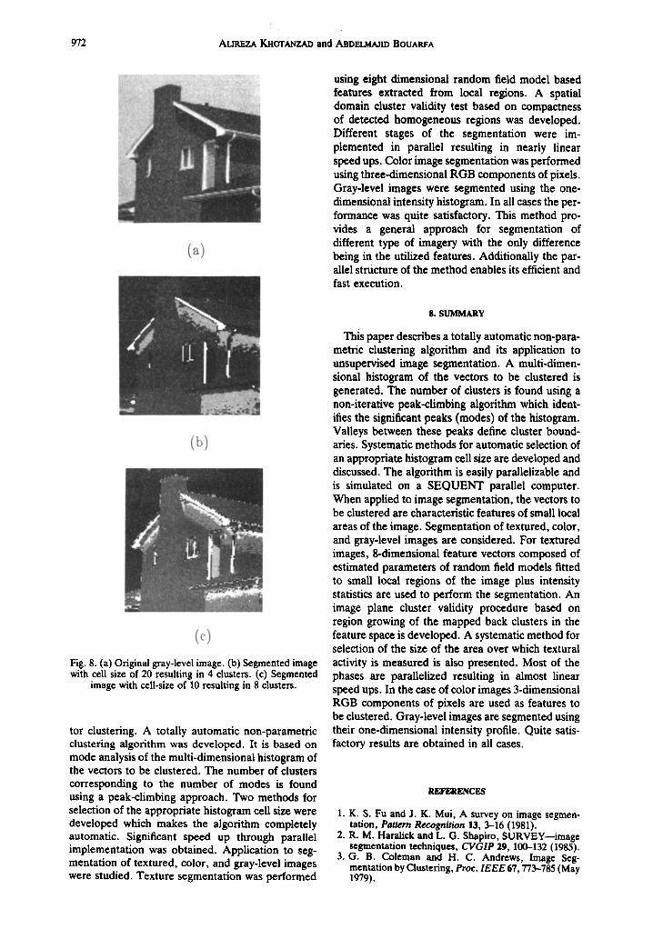
The last experiment concerns the segmentation of a gray level image. The considered feature is the pixel intensity in the 0-255 range. In this case, the procedure is one-dimensional and can be compared to segmentation by thresholding where a one-dimen- sional histogram is constructed and several thresholds are set according to the significant his- togram peaks corresponding to the distinct regions of the image. However, in the proposed method, only one parameter needs to be specified, namely, the cell size which in this one-dimensional case reduces to an interval. Like the previous case, this parameter is selected based on the desired seg- mentation resolution.
The gray level image to be segmented is shown in Fig. 8(a). Using two different cell sizes, 20 and 10, the resulting segmentations corresponding to 4 and 8 clusters respectively are presented in Figs 8(b) and 8(c). These two images show the effects of the cell
(b)
(c)
Fig. 7. (a) Original color image shown in black and white. The bird is mostly pink with a black area around its eyes and beak, the flowers are yellow, the leaves are green, and the background is a mixture of light yellow at the bottom and light blue on top. (b) Segmented image with cell size of 30 resulting in 4 clusters. (c) Segmented image with cell
size of 15 resulting in 10 clusters.
size on the quality of the segmentation~ More details are obtained as the cell size decreases since a smaller quantization enables the clustering procedure to dis- criminate smaller histogram peaks.
6. CONCLUSION
This paper focused on the problem of unsupervised image segmentation using characteristic feature vec-
972 ALJREZA KHOTANZAD and ABDELMAJID BOUARFA
¢.
/
(b)
(c) Fig. 8. (a) Original gray-level image. (b) Segmented image with cell size of 20 resulting in 4 clusters. (c) Segmented
image with cell-size of 10 resulting in 8 clusters.
tor clustering. A totally automatic non-parametric clustering algorithm was developed. It is based on mode analysis of the multi-dimensional histogram of the vectors to be clustered. The number of clusters corresponding to the number of modes is found using a peak-climbing approach. Two methods for selection of the appropriate histogram cell size were developed which makes the algorithm completely automatic. Significant speed up through parallel implementation was obtained. Application to seg- mentation of textured, color, and gray-level images were studied. Texture segmentation was performed
using eight dimensional random field model based features extracted from local regions. A spatial domain cluster validity test based on compactness of detected homogeneous regions was developed. Different stages of the segmentation were im- plemented in parallel resulting in nearly linear speed ups. Color image segmentation was performed using three-dimensional RGB components of pixels. Gray-level images were segmented using the one- dimensional intensity histogram. In all cases the per- formance was quite satisfactory. This method pro- vides a general approach for segmentation of different type of imagery with the only difference being in the utilized features. Additionally the par- allel structure of the method enables its efficient and fast execution.
8. S U I ~ Y
This paper describes a totally automatic non-para- metric clustering algorithm and its application to unsupervised image segmentation. A multi-dimen- sional histogram of the vectors to be clustered is generated. The number of clusters is found using a non-iterative peak-climbing algorithm which ident- ifies the significant peaks (modes) of the histogram. Valleys between these peaks define cluster bound- aries. Systematic methods for automatic selection of an appropriate histogram cell size are developed and discussed. The algorithm is easily parallelizable and is simulated on a SEQUENT parallel computer. When applied to image segmentation, the vectors to be clustered are characteristic features of small local areas of the image. Segmentation of textured, color, and gray-level images are considered. For textured images, 8-dimensional feature vectors composed of estimated parameters of random field models fitted to small local regions of the image plus intensity statistics are used to perform the segmentation. An image plane cluster validity procedure based on region growing of the mapped back clusters in the feature space is developed. A systematic method for selection of the size of the area over which textural activity is measured is also presented. Most of the phases are parallelized resulting in almost linear speed ups. In the case of color images 3-dimensional RGB components of pixels are used as features to be clustered. Gray-level images are segmented using their one-dimensional intensity profile. Quite satis- factory results are obtained in all cases.
R E F E R ~ C ~
1. K. S. Fu and J. K. Mui, A survey on image segmen- tation, Pattern Recognition 13, 3-16 (1981).
2. R. M. Haralick and L. G. Shapiro, SURVEY--image segmentation techniques, CVGIP 29, 100-132 (1985).
3. G. B. Coleman and H. C. Andrews, Image Seg- mentation by Clustering, Proc. IEEE 67, 773-785 (May 1979).
Image segmentation 973
4. R. Dubes and A. K. Jain, Validity studies in clustering methodologies, Pattern Recognition I1, 235-254 (1979).
5. A. K. Jain, Cluster Analysis, in Handbook of Pattern Recognition and Image Processing, pp. 33-57, Aca- demic Press, New York (1986).
6. P. M. Narendra and M. Goldberg, A non-parametric clustering scheme for LANDSAT, Pattern Recognition 9, 207-215 (1977).
7. S. W. Wharton, A generalized histogram clustering scheme for multidimensional image data, Pattern Rec- ognition 16, 193-199 (1983).
8. R. L. Kashyap and A. Khotanzad, A stochastic model based technique for texture segmentation, Proc. 7th Int. Conf. Pattern Recognition, Montreal, Canada, pp. 1202-1205 (30 July- 2 August 1984).
9. A. Khotanzad and J. Y. Chen, Unsupervised seg- mentation of textured image by edge detection in multi- dimensional feature, 1EEE Trans. Pattern Anal. Mach. lntell. PAMI-11,414--421 (April 1989).
10. A. Khotanzad and R. L. Kashyap, Feature selection for texture recognition using image synthesis, IEEE Trans. Syst. Man Cybern. 17, 1087--1095 (November 1987).
11. W. Koontz, P. M. Narendra and K. Fukunaga, A graph theoretic approach to non-parametric cluster analysis, 1EEE Trans. Comput. C-2S, 936-944 (1976).
12. F. R. Fromm and R. A. Nortbouse, CLASS: A Non- parametric clustering algorithm, Pattern Recognition 8, 107-114 (July 1976).
13. J. M. Coggins and A. K. Jain, A spatial filtering approach to texture analysis, Pattern Recognition Len. 3, 195--203 (1985).
14. R. L. Kashyap and R. Chellappa, Estimation and choice of neighbors in spatial interaction models of images, IEEE Trans. Inform. Theory IT-29, 60-72, (1983).
15. P. Brodatz, Texture: A Photographic AIbum for Artists and Designers, Dover, New York (1956).
About the AuthormALIREZA KHOTANZAD was born in Tehran, Iran, in 1956. He received the B,S., M.S., and Ph.D. degrees in Electrical Engineering from Purdue University, West Lafayette, Indiana, in 1978, 1980, and 1983, respectively. In 1984 he joined the faculty of the Department of Electrical Engineering, Southern Methodist University, Dallas, Texas, where he is now an Associate Professor. His research interest are in the areas of computer vision, pattern recognition, neural networks, and texture analysis.
About the Author--ABDELMAJID BOUARFA received the Engineer degree in Electrical Engineering from Ecole Nationale Polytechnique of Algiers, Algeria in 1982 and his M.S. and Ph.D. degrees in Electrical Engineering from Southern Methodist University in 1984 and 1989, respectively.
His domain of interest is in image processing and pattern recognition and his research activities center around texture and cluster analysis.
Related Documents