Human Capital Formation, Life Expectancy and the …ftp.iza.org/dp585_ov.pdf · Human Capital Formation, Life Expectancy and the Process of Economic Development Matteo Cervellati

Human Capital Formation, Life Expectancy and the Process of

Economic Development

Matteo Cervellati Universitat Pompeu Fabra, Barcelona and University of Bologna

Uwe Sunde

IZA Bonn and University of Bonn

Discussion Paper No. 585 September 2002

IZA

P.O. Box 7240 D-53072 Bonn

Germany

Tel.: +49-228-3894-0 Fax: +49-228-3894-210

Email: [email protected]

This Discussion Paper is issued within the framework of IZA’s research area Welfare State and Labor Market. Any opinions expressed here are those of the author(s) and not those of the institute. Research disseminated by IZA may include views on policy, but the institute itself takes no institutional policy positions. The Institute for the Study of Labor (IZA) in Bonn is a local and virtual international research center and a place of communication between science, politics and business. IZA is an independent, nonprofit limited liability company (Gesellschaft mit beschränkter Haftung) supported by the Deutsche Post AG. The center is associated with the University of Bonn and offers a stimulating research environment through its research networks, research support, and visitors and doctoral programs. IZA engages in (i) original and internationally competitive research in all fields of labor economics, (ii) development of policy concepts, and (iii) dissemination of research results and concepts to the interested public. The current research program deals with (1) mobility and flexibility of labor, (2) internationalization of labor markets, (3) welfare state and labor market, (4) labor markets in transition countries, (5) the future of labor, (6) evaluation of labor market policies and projects and (7) general labor economics. IZA Discussion Papers often represent preliminary work and are circulated to encourage discussion. Citation of such a paper should account for its provisional character. A revised version may be available on the IZA website (www.iza.org) or directly from the author.

IZA Discussion Paper No. 585 September 2002

ABSTRACT

Human Capital Formation, Life Expectancy and the Process of Economic Development

This paper presents a microfounded theory of long-term development. We model the interplay between economic variables, namely the process of human capital formation and technological progress, and the biological constraint of finite lifetime expectancy. All these processes affect each other and are endogenously determined. The model is analytically solved and simulated for illustrative purposes. The resulting dynamics reproduce a long period of stagnant growth as well as an endogenous and rapid transition to a situation characterized by permanent growth. This transition can be interpreted as industrial revolution. Historical and empirical evidence is discussed and shown to be in line with the predictions of the model. JEL Classification: E10, J10, O10, O40, O41 Keywords: long-term development, endogenous lifetime duration, endogenous life

expectancy, human capital, technological progress, growth externalities, industrial revolution

Corresponding author: Uwe Sunde Institute for the Study of Labor (IZA) PO Box 7240 53072 Bonn Germany Tel.: +49 228 3894 533 Fax: +49 228 3894 210 Email: [email protected]

The authors would like to thank Antonio Ciccone, Adriana Kugler, Matthias Messner and Nicola Pavoni for helpful comments. Financial support from German Research Foundation DFG, and IZA is gratefully acknowledged. All errors are our own.

1 Introduction

The past two centuries were characterized by widespread and profoundchanges in human living conditions. For aeons, a more or less stable and un-changed environment prevailed, with a strong preponderance of agricultureand trade of basic goods, rigid social structures with usually a small rulingclass, and comparably poor medical conditions. But suddenly within justmore than two hundred years, that is just a few generations, the economicenvironment mutated utterly as the structure of the economy completelychanged with industrialization breaking its way, reducing the importanceof agricultural activities in favor of the industrial and the service sector.Personal life changed in every dimension to an extent not seen before orafter. The traditional social environment ceased to exist, as the vast ma-jority of the population became educated, and acquired knowledge beyondthe working knowledge of performing a few manual tasks inherited by pre-vious generations. Literacy, which used to be the privilege of a little elite,became widespread among the population. The process of human capitalaccumulation accelerated as more and more people acquired the ability toinnovate, and to use innovations. On the other hand, the spread of newtechnologies in turn made it more profitable to acquire knowledge. Also thebiological environment sharply changed. Lifetime duration, which had beenvirtually the same for thousands of years, increased sharply within just a fewgenerations. Mortality fell significantly and fertility behavior changed pro-foundly, hygienic conditions improved as sanitation became more importantand widespread.

Economists have always had a great interest in understanding the rea-sons and the mechanics of these dramatic changes, in particular against thebackground of the fact that large parts of the world are still underdevel-oped. Several recent contributions address the issue of the economic tran-sition from stagnant, Malthusian regimes to permanent growth, like Good-friend and McDermott (1995), Hansen and Prescott (1998), Lucas (2002),Galor and Weil (2000), Galor and Moav (2001), Jones (2001) and Jones(2002). The driving forces, which explain the economic transition towardshigher growth paths in these models, are technical progress, physical capitalaccumulation, and, most importantly, the process of human capital accu-mulation. The analyzed decision processes also affect fertility behavior andare capable of producing an endogenous demographic transition towards aregime of lower population growth. However, in the light of the changesin personal living conditions that accompanied the economic developments,also lifetime duration played a crucial role in the process of development.But, as some authors like Mokyr (1993) already pointed out, two separatestrands of the literature, one about the causes and mechanics of the indus-trial revolution, and another about the decline in mortality, largely coexistwithout any obvious connection or compatibility between the two.

2

Some recent contributions explicitly include mortality or lifetime dura-tion to explain the mechanism of economic development. Kalemli-Ozcanet al. (2000) develop a general equilibrium model to study the effects ofexogenous changes in mortality on schooling and human capital accumu-lation. Croix and Licandro (1999), Boucekkine, de la Croix, and Licandro(2002a) and Boucekkine, de la Croix, and Licandro (2002b) consider endoge-nous growth models in which life expectancy is exogenous and affects thelevel of schooling, which in turn determines growth. Swanson and Kopecky(1999) present cross-country evidence for the relevance of life expectancy ongrowth, and develop a model of human capital accumulation in which indi-viduals have a finite lifespan. Reis-Soares (2001) explores the link betweenlife expectancy, educational attainment and fertility choice in the context oflong-run development, and presents cross-country evidence for interactionsbetween life expectancy, income, schooling levels and fertility.

All these contributions emphasize that lifetime duration plays a crucialrole for human capital investments, which in turn determine growth. More-over, the empirical evidence they present or cite, strongly supports thisview. However, while these models acknowledge the importance of lifetimeduration for human capital accumulation and growth, they neglect poten-tial reverse effects of development on lifetime duration. There is now generalagreement in the fields of economic history and demography that economicdevelopment and the level of human capital profoundly affects lifetime du-ration and living conditions. A large body of empirical evidence supportsthe view that higher levels of development are correlated with longer lifeexpectancy. This evidence suggests that traditionally little education andknowledge about health and means to avoid illness supported the outbreak,propagation and mal-treatment of diseases and ultimately led to high mor-tality. However, an increasing popular knowledge of the treatment of com-mon diseases and about the importance of hygiene and sanitation, as well asthe availability of respective technologies, helped to increase life expectancysomewhat over time (see Mokyr, 1993). There is also evidence for an inverserelation between parents’ schooling and child mortality, suggesting that lifeexpectancy increases in parents’ human capital. Evidently, a mother’s levelof education has positive effects on life expectancy of her children (Schultz,1993). The invention of new drugs, which depends crucially on the hu-man capital involved in research, increased life expectancy (see Lichtenberg,1998). Blackburn and Cipriani (2002) cite further empirical evidence for theview that life expectancy depends on economic conditions. Moreover, theydevelop a model with endogenous life expectancy, in which the economymay end up in different development regimes, depending on the initial con-ditions. Similarly, Kalemli-Ozcan (2002) shows the possibility for multipleequilibria in a model in which individuals decide upon their fertility and theeducation of their children, once life expectancy is seen as endogenous anddepending on income per capita.

3

Hence, there is little dispute in the literature that life expectancy isa crucial determinant of human capital accumulation and economic devel-opment, and that the level of human capital and development in generalaffects lifetime duration. However, in the context of the early stages of theindustrial revolution issues are still largely unsettled. From the late 18thcentury onwards mortality decreased. In the same period, literacy began tospread and growth started to accelerate with the invention of new productiontechnologies. The question which factor was primarily responsible for theseprofound changes is still hotly debated. Some authors explain the declinein mortality and the increase in life expectancy by increases in householdincomes and technological progress (see e. g. McKeown, 1977). However,this view has been criticized on the basis of the empirical evidence, whichsuggests that technological (medical) progress took off too late to explainearly increases in lifetime duration. Moreover, by and large, the standard ofliving in terms of income, housing and nutrition of the majority of the pop-ulation hardly changed before 1850, indicating that this explanation doesnot tell the entire story, see Mokyr (1993). Others, like Boucekkine, de laCroix, and Licandro (2002b) and the references therein, argue that alreadyat the dawn of the industrial revolution mortality declined. This decline isviewed as an exogenous event, which in turn triggered more investment inhuman capital and faster growth. Subsequent changes in mortality, however,are again interpreted as endogenous consequences of economic development,leaving the cause of the industrial revolution essentially unexplained. Thereis a strong disagreement among conomic historians like Riley (2001) andEasterlin (2002) about whether the onset of increases in life expectancy canbe precisely dated for different countries. There is a similar disagreementwhether this onset coincided with the beginning of the industrial revolutionand the transition to a faster regime of growth, or whether changes in lifeexpectancy preceeded or followed changes in the economic environment.

The contribution of this paper is to provide a unified framework to an-alyze the interactions between human capital accumulation, technologicalprogress and lifetime duration in the context of long term development, inwhich all these relevant processes are determined endogenously. The modelto be presented has three basic building blocks. The first block is a micro-founded model of human capital formation in which heterogeneous individu-als decide upon the type and the amount of human capital to acquire duringtheir lives. This optimal choice depends crucially on their life expectancyand the state of technology. The second block is the idea that human capitalis the primary engine of economic growth. Human capital affects the stateof technology in terms of factor productivity in the aggregate productionprocess. The resulting technical progress makes future investments in hu-man capital more profitable. The third block is motivated by the historicaland demographic evidence mentioned above and concerns the effects of theeconomic and social environment on lifetime duration. In particular, the

4

evolution of life expectancy is endogenously linked to the process of humancapital accumulation.

The main mechanism of the model to be presented below can be summa-rized as follows. Individuals maximize their lifetime utility by their choiceof human capital accumulation. This decision shapes the structure of theeconomy during their lives. In their choice, individuals take their expectedlifetime duration as given, and they do not consider the effect of their de-cision on the life expectancy of future generations. This in turn creates anexternality on future human capital decisions. Moreover, the level of humancapital created by a generation of individuals affects productivity and there-fore the growth potential of the economy in the future. In principle, thereis a virtuous cycle of human capital accumulation and growth. However,as long as the biological barrier of low life expectancy is binding, develop-ment of the economy will be very slow. The economy is virtually trappedon a slow growth path. Eventually, once average life lifetime duration ishigh enough and the level of technology is sufficiently advanced to inducelarge proportions of the population to acquire high quality human capital,growth takes off. A phase of fast development and a profound change inthe structure of economy, which can be interpreted as an industrial revolu-tion, starts, and the economy converges within a few generations to a newpath with higher growth rates than before. As a consequence of the increasein life expectancy, population size grows even though fertility behavior isunchanged.

The paper is organized as follows. In section 2 we describe the individualproblem of human capital accumulation in the face of given technologies, aswell as the economic environment, and solve for the intragenerational equi-librium. The intertemporal links between subsequent generations, and theprocess of dynamic development are presented in section 3. There, we alsopresent the main result, a characterization of long-term development. Sec-tion 4 contains simulations of the model to illustrate how it can account forthe long-run development experience. Moreover, in this section we comparethe implications of the model with empirical evidence and present possibleextensions and generalizations. Section 5 concludes. All proofs are collectedin the appendix.

2 Intragenerational Human Capital Formation

The economy is populated by an infinite sequence of non-overlapping gen-erations of individuals.1 In this section we analyze the process of humancapital formation, goods production, and we study the intragenerationalequilibrium. The next section deals with the links between generations andanalyzes the evolution of the dynamic system.

1An extension to a framework with overlapping generations is presented in section 4.3.

5

We start by looking at the individual problem of investing in humancapital. The types of human capital at disposal differ in the way theyare built up, and in the returns individuals receive from them. The maininputs in building up human capital are individual ability and time spent foreducation. From the individual point of view, the time available is limitedby the expected lifetime duration, which is therefore taken as given by theindividual. The same is true for the returns to human capital, which aredetermined on competitive markets at the aggregate level. The individualproblem is then which type of human capital to acquire and how much ofit. The intragenerational equilibrium is characterized by the interplay ofindividual optimizing behavior and aggregate market conditions.

2.1 Production of Human Capital

A generation consists of a continuum of agents with population size nor-malized to one. Every individual is endowed with ability a ∈ [a, a] and theexogenous distribution of ability in the population is f (a).

In order to make an income, individuals have to spend their ability andsome of their living time to form some human capital. There are severaltypes of human capital, which differ with respect to their production pro-cess and the returns they generate. For simplicity, we concentrate on thesimple case of only two types of human capital. Along the lines of growththeory, one type of human capital is interpreted as high-quality, and growthenhancing. This type is labelled theoretical human capital and is denotedby h. This type of human capital is the primary engine of modern economicgrowth. It is characterized by a high content of abstract knowledge. Thistype of human capital is important for innovation and development of newideas, since abstract knowledge helps to solve a problem never faced beforeby resorting to known abstract concepts.

The second type is labelled applied human capital, denoted by p, andcan be interpreted as labor capacity. It contains less intellectual quality,but more manual and practical skills that are important in performing tasksrelated to existing technologies.2

Both types of human capital are produced using time e and individualability a as inputs:

p = fp(e, a) , and h = fh (e, a)

These production processes are inherently different. The levels of bothtypes of human capital increase in the time spent in forming them. Themain difference lies in the effectiveness of time. To acquire theoretical hu-man capital h, it is necessary to first spend time on the building blocks

2In the language of labor economics, theoretical human capital could be associatedwith skilled labor, while applied human capital is associated with unskilled labor.

6

of the elementary concepts without being productive in the narrow sense.This view of human capital formation is in line with the mastery learningconcept as understood by for example Becker, Murphy, and Tamura (1990),which states that learning complicated materials is more efficient when theelementary concepts are mastered. Once the basic concepts are internal-ized, the time spent on theoretical human capital is very productive. Onthe contrary, the time devoted to acquire applied human capital p is imme-diately effective, albeit with a lower overall productivity. Personal ability isrelatively more important in acquiring theoretical human capital.

Formally, the following production functions exhibit these different char-acteristics of the processes of building up human capital:

h =

α(e − e)a if e ≥ e0 if e < e

(1)

andp = βe . (2)

In order to acquire theoretical human capital h, an agent needs to paya fix cost e measured in time units while for applied human capital p thefix cost is smaller and normalized to zero.3 Any unit of time produces αunits of h and β units of p with α ≥ β. Ability is modeled as increasing theproduction of human capital h per unit of time.

2.2 The Individual Human Capital Investment Problem

There is just one consumption good in the economy. Strictly speaking,agents face an intertemporal problem of maximizing their lifetime utility.According to lifecycle consumption theory, with concave utility, positivediscount rate and perfect capital markets, an agent consumes in every perioda fixed amount that depends on the stream of discounted lifetime earnings.In this case, it is sufficient for agents to maximize total lifetime earningsin order to maximize their individual lifetime utility, see e.g. Galor andMoav (2000). Thus the lifetime utility is maximized by choosing optimallythe type of human capital to acquire and the time e spent producing it.We abstract from life cycle considerations and normalize the discount factorto zero, so agents are indifferent with respect to the date of consumption.Individuals are assumed to neither receive nor leave bequests.

Since building up human capital takes time, individuals face an intertem-poral trade-off between spending time on building human capital and spend-ing time and using the acquired human capital on working and earning in-come. While accumulating human capital, agents cannot work. This means

3We abstract from other costs of education, like tuition fees etc. Moreover, the fixedcost is assumed to be constant and the same for every generation. Costs that increaseor decrease along the evolution of generations would leave the qualitative results of thepaper unchanged.

7

that agents must optimally decide how to split their expected lifetime be-tween human capital formation and work. We abstract from leisure andlearning on-the-job.

This setting is chosen to catch two crucial features of the human capitalformation process. The first one is that larger lifetime duration induces in-dividuals to acquire more of any type of human capital. The second featureis that increasing lifetime duration makes theoretical, high quality humancapital relatively more attractive for individuals of any level of ability. Anyalternative model of human capital formation reproducing these two fea-tures would be entirely equivalent for the purpose of this paper. Alternativesettings like learning on-the-job could similarly be used to illustrate theimportance of lifetime duration for human capital formation.

An agent can either decide to acquire h or p but not both. Formally,in his choice, he takes lifetime duration T as well as the wages for unit ofhuman capital, wh and wp, as given. Lifetime utility in the two cases is thengiven by the product of the length of the working life, the amount of humancapital one has acquired, and the wage rate per unit of human capital perunit of time:

Vh (eh, a) = (T − eh) hwh

= (T − eh) α(eh − e)awh , , and (3)

Vp (ep, a) = (T − ep) pwp

= (T − ep) βepwp . (4)

To maximizes his lifetime utility, an agent compares the maximum life-time utility he can get by acquiring one type of human capital or the other.Consequently, he chooses to acquire p or h depending on whether:

V ∗p

(e∗p, a, wp

) >< V ∗

h (e∗h, a, wh) ,

where:

e∗h = arg maxVh (eh, a, wh) = (T − eh) α(e − e)awh ,

ande∗p = arg maxVp (ep, a, wp) = (T − ep) βepwp .

The optimal time investments are then given by:

e∗h =T + e

2, and e∗p =

T

2,

respectively.

8

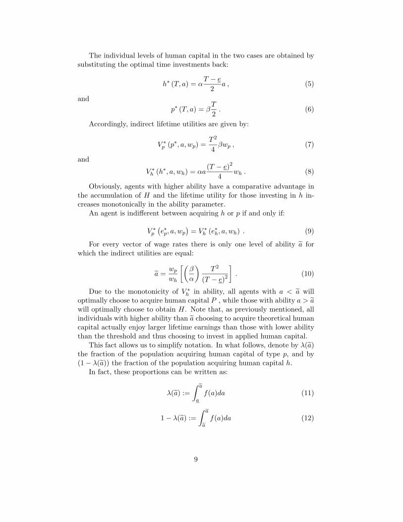
The individual levels of human capital in the two cases are obtained bysubstituting the optimal time investments back:

h∗ (T, a) = αT − e

2a , (5)

andp∗ (T, a) = β

T

2. (6)

Accordingly, indirect lifetime utilities are given by:

V ∗p (p∗, a, wp) =

T 2

4βwp , (7)

and

V ∗h (h∗, a, wh) = αa

(T − e)2

4wh . (8)

Obviously, agents with higher ability have a comparative advantage inthe accumulation of H and the lifetime utility for those investing in h in-creases monotonically in the ability parameter.

An agent is indifferent between acquiring h or p if and only if:

V ∗p

(e∗p, a, wp

)= V ∗

h (e∗h, a, wh) . (9)

For every vector of wage rates there is only one level of ability a forwhich the indirect utilities are equal:

a =wp

wh

[(β

α

)T 2

(T − e)2

]. (10)

Due to the monotonicity of V ∗h in ability, all agents with a < a will

optimally choose to acquire human capital P , while those with ability a > awill optimally choose to obtain H. Note that, as previously mentioned, allindividuals with higher ability than a choosing to acquire theoretical humancapital actually enjoy larger lifetime earnings than those with lower abilitythan the threshold and thus choosing to invest in applied human capital.

This fact allows us to simplify notation. In what follows, denote by λ(a)the fraction of the population acquiring human capital of type p, and by(1 − λ(a)) the fraction of the population acquiring human capital h.

In fact, these proportions can be written as:

λ(a) :=∫

a

af(a)da (11)

1 − λ(a) :=∫ a

af(a)da (12)

9

By inspection of equation (10) and since T − e > 0, one can see that thefraction 1 − λ(a) increases with lifetime duration T , with the relative wagewhwp

and with αβ .

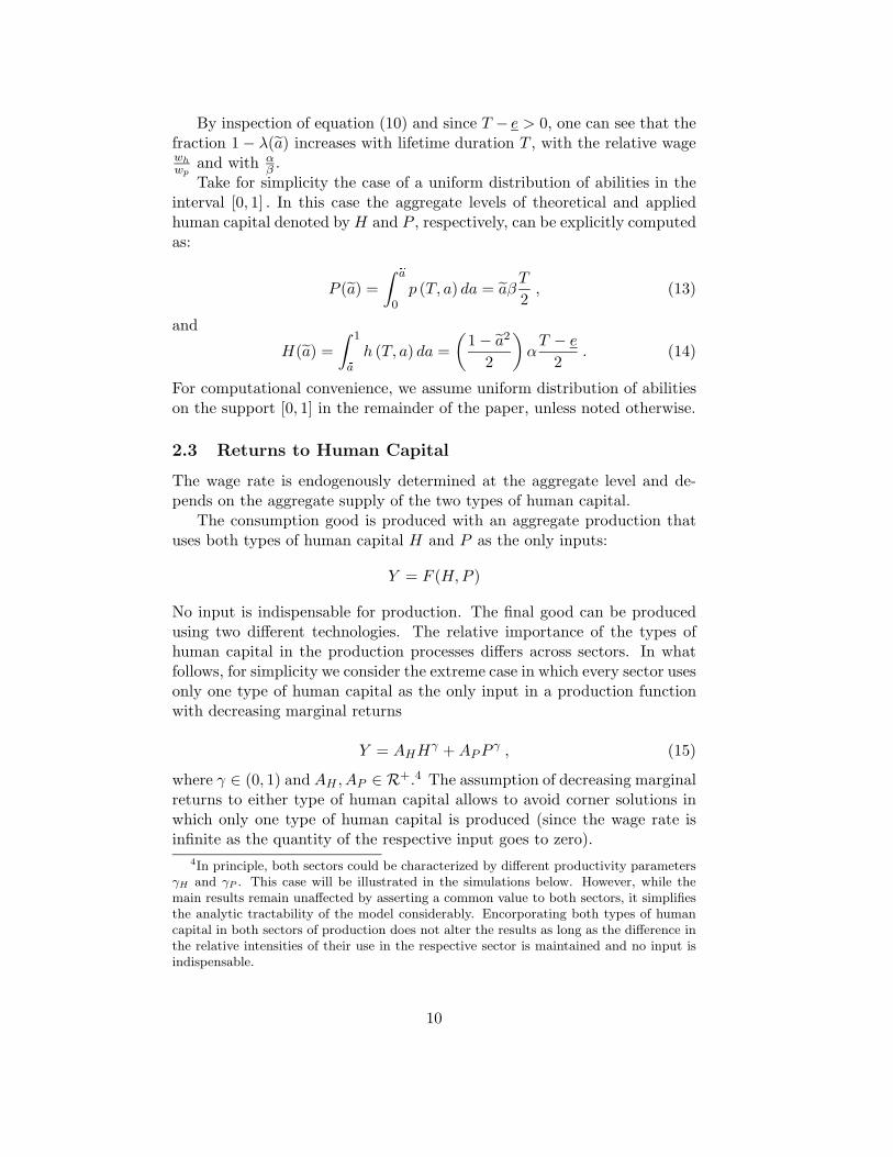
Take for simplicity the case of a uniform distribution of abilities in theinterval [0, 1] . In this case the aggregate levels of theoretical and appliedhuman capital denoted by H and P , respectively, can be explicitly computedas:

P (a) =∫

a

0p (T, a) da = aβ

T

2, (13)

and

H(a) =∫ 1

ah (T, a) da =

(1 − a2

2

)α

T − e

2. (14)

For computational convenience, we assume uniform distribution of abilitieson the support [0, 1] in the remainder of the paper, unless noted otherwise.

2.3 Returns to Human Capital

The wage rate is endogenously determined at the aggregate level and de-pends on the aggregate supply of the two types of human capital.

The consumption good is produced with an aggregate production thatuses both types of human capital H and P as the only inputs:

Y = F (H, P )

No input is indispensable for production. The final good can be producedusing two different technologies. The relative importance of the types ofhuman capital in the production processes differs across sectors. In whatfollows, for simplicity we consider the extreme case in which every sector usesonly one type of human capital as the only input in a production functionwith decreasing marginal returns

Y = AHHγ + AP P γ , (15)

where γ ∈ (0, 1) and AH , AP ∈ R+.4 The assumption of decreasing marginalreturns to either type of human capital allows to avoid corner solutions inwhich only one type of human capital is produced (since the wage rate isinfinite as the quantity of the respective input goes to zero).

4In principle, both sectors could be characterized by different productivity parametersγH and γP . This case will be illustrated in the simulations below. However, while themain results remain unaffected by asserting a common value to both sectors, it simplifiesthe analytic tractability of the model considerably. Encorporating both types of humancapital in both sectors of production does not alter the results as long as the difference inthe relative intensities of their use in the respective sector is maintained and no input isindispensable.

10

Factors of production are sold in the competive market and receive wagesequal to their marginal productivity. Thus, the wage rate ratio that iscompatible with the macroeconomic equilibium is:

wp

wh=

AP P γ−1

AHHγ−1. (16)

2.4 Intragenerational Equilibrium

Given this setting, we can define the intragenerational equilibrium of thiseconomy as follows:

Definition 1. The intragenerational equilibrium is a vector:w∗

h, w∗P , a∗, H∗, P ∗, h∗(T, a)a∈[a,a] , p∗(T, a)a∈[a,a]

such that, for any given T and distribution f (a) we have:

h∗ (T, a) = αT − e

2a , ∀a ≥ a∗ (17)

p∗ (T, a) = βT

2∀a < a∗ (18)

H∗ =∫ a

a∗h∗ (T, a) f(a)da (19)

P ∗ =∫

a∗

ap∗ (T, a) f(a)da (20)

w∗h = AHγH∗γ−1 (21)

w∗p = AP γP ∗γ−1 (22)

a∗ =w∗

p

w∗h

[(β

α

)T 2

(T − e)2

](23)

The equilibrium system (17) to (23) defines an implicit function in (a∗, T )linking the equilibrium cut-off level of ability a∗ to lifetime duration T .Since,

w∗p

w∗h

=AP γP ∗γ−1

AHγH∗γ−1=

[(α

β

)(T − e)2

T 2

]a∗ =

w∗p

w∗h

. (24)

Substituting for P (a∗), H(a∗) from Equation (13) and (14) we have:

a∗(

(1 − a∗2)2a∗

)γ−1

=AP

AH

(β

α

)γ ( T

T − e

)γ+1

(25)

This relation between the equilibrium ability threshold for the acqui-sition of abstract human capital and life expectancy T will be of eminent

11

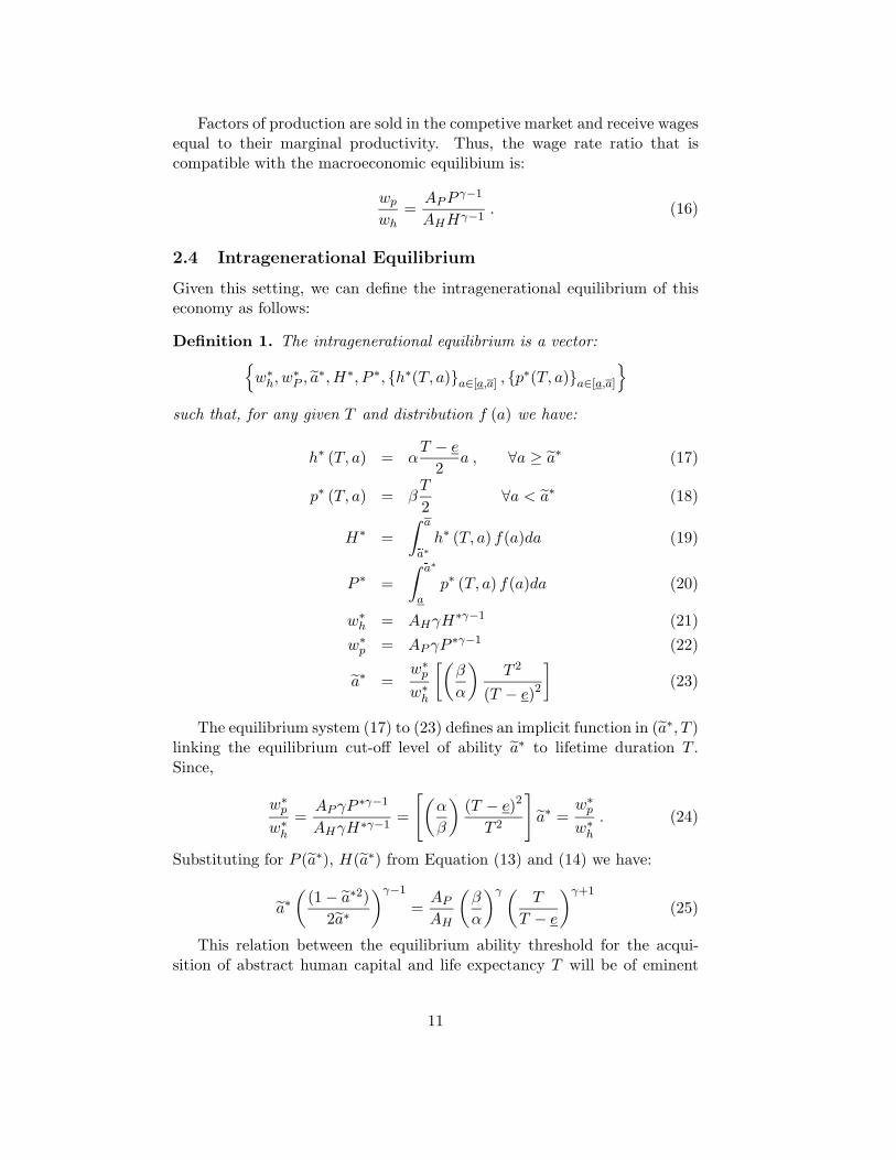
importance for the analysis of development later on. For notational con-venience, reformulate Equation (25) by solving for lifetime expectancy as afunction of the ability threshold to get:

T (a∗) =e

1 − g(a∗)Ω

, (26)

with

g(a∗) =(1 − a∗2)

1−γ1+γ

a∗ 2−γ

1+γ

k , (27)

k = 2−1−γ1+γ , and

Ω =[(

AH

AP

)(α

β

)γ] 11+γ

: . (28)

It is easy to see that g(a∗) > 0, ∀a ∈ [0, 1]. Note that T (a∗) is definedfor all a∗ ∈ [a∗, 1] with a∗ : g(a∗) = Ω ⇔ lim

a∗→a∗ T (a∗) = ∞, and that∀a∗ ∈ [a∗, 1] : 1 − g(a∗)

Ω > 0. The value a∗ > 0 represents a maximumfraction of the population that would optimally choose to acquire humancapital H for any given level of relative productivity AH

AP. This maximum

fraction cannot be exceeded, even if the biological constraint of finite lifetimeduration would disappear (i. e. if T = ∞).

There exists a unique pair of expected lifetime duration and ability thatsatisfies the conditions for an intragenerational equilibrium:

Proposition 1. There exists exactly one intragenerational equilibrium char-acterized by the a pair (a∗, T ∗), with a∗ ∈ [a∗ (Ω) , 1] and T ∈ [e,∞), whichsatisfies condition (25).

In this context, it is worth noting that the maximum proportion of thepopulation that would acquire H in the absence of biological constraints,1 − a∗ (Ω) , is increasing with the relative productivity of the sector usingtheoretical human capital intensively, AH

AP. This observation will prove useful

later on and is therefore summarized in:

Lemma 1. The lower bound on the support of ability thresholds decreasesas Ω increases, that is ∂a∗(Ω)

∂Ω < 0.

2.5 Properties of the Intragenerational Equilibrium

The equilibrium relation between lifetime duration and the proportion ofthe population investing in human capital presented in equation (25) will bea crucial determinant of the dynamic system. This relation is determinedendogenously for a given generation through the interplay of individual op-timizing behavior and aggregate equilibrium conditions. According to thefollowing proposition, the ability cut-off is lower for higher expected lifetime

12

duration, that means that a higher share of the population decides to ob-tain human capital of type h if they expect to live longer. Moreover, thefunction a∗ (T ), representing the threshold ability defining the proportionof the population acquiring human capital h, is S-shaped: as lifetime dura-tion increases the proportion of population choosing h increases first slowly,then increasingly rapidly, until this increase slows down again as the abilitythreshold converges to ever lower levels.

Proposition 2. The cut-off level a∗ (T ), which identifies the equilibriumfraction of members of a generation acquiring human capital h, is an in-creasing, S-shaped function of expected lifetime duration T of this genera-tion, with zero slope for T −→ 0 and T −→ ∞, and exacly one inflectionpoint.

The full proof is contained in the appendix. The economic meaning be-hind the S-shape is easier to grasp when looking at the equilibrium relationin the (λ, T )-space. The equilibrium locus can be rationalized as follows. Forlow lifetime durations, the share of population investing in h is small, andalso relatively large increases in average lifetime duration do not change thisstructure of the economy much. The reason for this is that due to the fixedcost involved with acquiring h, the remaining time to use the acquired h toearn income is too short for a large part of the population to be worth theeffort. Once average lifetime duration increases sufficiently, the fixed costconstraint binds for fewer and fewer people, so the structure of the economychanges more rapidly towards a higher fraction of people acquiring h. How-ever, the speed of this structural change decreases as an ever larger shareof the population is engaged in h due to decreasing returns in both sectors:Since only few individuals decide to invest in p the relative wage wh/wp

decreases affecting the individual choice of human capital accumulation.Lifetime duration therefore constrains the development of the economy.

The smooth convergence of a small proportion of people investing in h at lowlifetime durations is due to the fixed costs related to it. On the other hand,the fact that there is always a small portion of the population investing in peven for high average lifetime durations has to do with decreasing marginalreturns to h and p.

Having characterized the static behavior of the economy, we now turnto the dynamic process of development.

3 The Process of Economic Development

In the economy described in the previous section, lifetime duration is con-sidered as given the individual point of view. The structure of the economyin every generation is the outcome of individual decisions and depends onaverage expected lifetime duration. On the other hand, in the long run and

13

from a macroeconomic perspective, lifetime duration is endogenous. Ex-pected lifetime duration is related to the level of development through thestructure of the economy. This section models the intertemporal interplaybetween these two mechanisms characterizing the development path of aneconomy starting from an initial situation with low average lifetime dura-tion.

Let us consider an economy with an infinite number of successive gener-ations with identical stationary distributions of innate ability.5 Generationswill be denoted with subscript t. Every agent in a given generation faces adecision regarding the accumulation of human capital identical to the onedescribed previously. Every generation has to build up the stock of humancapital capital from zero, since the peculiar characteristic of human capitalis that it is embodied in people (even if the production can be easier if theprevious generation had a lot of it).6 In order to isolate the developmenteffects related to lifetime duration and human capital accumulation, anylinks between generations through savings or bequests are excluded.

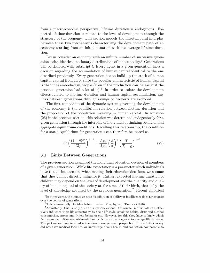
The first component of the dynamic system governing the developmentof the economy is the equilibrium relation between lifetime duration andthe proportion of the population investing in human capital. In equation(25) in the previous section, this relation was determined endogenously for agiven generation through the interplay of individual optimizing behavior andaggregate equilibrium conditions. Recalling this relationship, the conditionfor a static equilibrium for generation t can therefore be stated as:

a∗t

((1 − a∗2t )

2a∗t

)γ−1

=AP.t

AH.t

(β

α

)γ ( Tt

Tt − e

)γ+1

(29)

3.1 Links Between Generations

The previous section examined the individual education decision of membersof a given generation. While life expectancy is a parameter which individualshave to take into account when making their education decisions, we assumethat they cannot directly influence it. Rather, expected lifetime duration ofchildren may depend on the level of development and the quantity and qual-ity of human capital of the society at the time of their birth, that is by thelevel of knowledge acquired by the previous generation.7 Recent empirical

5In other words, the innate ex ante distribution of ability or intelligence does not changeover the course of generations.

6This is essentially the idea behind Becker, Murphy, and Tamura (1990).7Admittedly, this is only true to a certain extent. Of course, individuals can effec-

tively influence their life expectancy by their life style, smoking habits, drug and alcoholconsumption, sports and fitness behavior etc. However, for this they have to know whichfactors and activities are detrimental and which are advantageous for average life duration.The picture we have in mind is therefore more general: people born in the 18th centurydid not have medical facilities, or knowledge about health and sanitation comparable to

14

findings show that the level of GDP and literacy are positively correlatedwith average expected lifetime duration (see Swanson and Kopecky, 1999,and Reis-Soares, 2001 ). Of course, this effect has also an impact on thechildren’s decision of which type of human capital to acquire, as will becomeclear below.

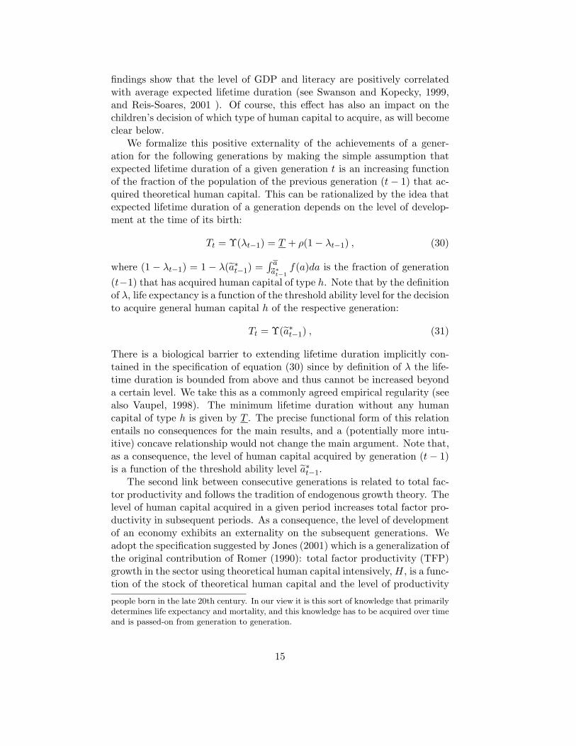
We formalize this positive externality of the achievements of a gener-ation for the following generations by making the simple assumption thatexpected lifetime duration of a given generation t is an increasing functionof the fraction of the population of the previous generation (t − 1) that ac-quired theoretical human capital. This can be rationalized by the idea thatexpected lifetime duration of a generation depends on the level of develop-ment at the time of its birth:

Tt = Υ(λt−1) = T + ρ(1 − λt−1) , (30)

where (1 − λt−1) = 1 − λ(a∗t−1) =∫ aa∗

t−1f(a)da is the fraction of generation

(t−1) that has acquired human capital of type h. Note that by the definitionof λ, life expectancy is a function of the threshold ability level for the decisionto acquire general human capital h of the respective generation:

Tt = Υ(a∗t−1) , (31)

There is a biological barrier to extending lifetime duration implicitly con-tained in the specification of equation (30) since by definition of λ the life-time duration is bounded from above and thus cannot be increased beyonda certain level. We take this as a commonly agreed empirical regularity (seealso Vaupel, 1998). The minimum lifetime duration without any humancapital of type h is given by T . The precise functional form of this relationentails no consequences for the main results, and a (potentially more intu-itive) concave relationship would not change the main argument. Note that,as a consequence, the level of human capital acquired by generation (t − 1)is a function of the threshold ability level a∗t−1.

The second link between consecutive generations is related to total fac-tor productivity and follows the tradition of endogenous growth theory. Thelevel of human capital acquired in a given period increases total factor pro-ductivity in subsequent periods. As a consequence, the level of developmentof an economy exhibits an externality on the subsequent generations. Weadopt the specification suggested by Jones (2001) which is a generalization ofthe original contribution of Romer (1990): total factor productivity (TFP)growth in the sector using theoretical human capital intensively, H, is a func-tion of the stock of theoretical human capital and the level of productivity

people born in the late 20th century. In our view it is this sort of knowledge that primarilydetermines life expectancy and mortality, and this knowledge has to be acquired over timeand is passed-on from generation to generation.

15

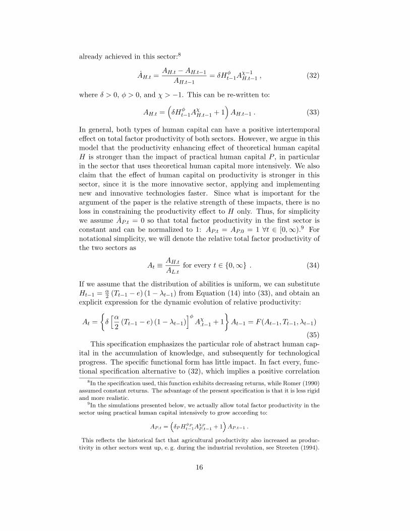
already achieved in this sector:8

AH.t =AH.t − AH.t−1

AH.t−1= δHφ

t−1Aχ−1H.t−1 , (32)

where δ > 0, φ > 0, and χ > −1. This can be re-written to:

AH.t =(δHφ

t−1AχH.t−1 + 1

)AH.t−1 . (33)

In general, both types of human capital can have a positive intertemporaleffect on total factor productivity of both sectors. However, we argue in thismodel that the productivity enhancing effect of theoretical human capitalH is stronger than the impact of practical human capital P , in particularin the sector that uses theoretical human capital more intensively. We alsoclaim that the effect of human capital on productivity is stronger in thissector, since it is the more innovative sector, applying and implementingnew and innovative technologies faster. Since what is important for theargument of the paper is the relative strength of these impacts, there is noloss in constraining the productivity effect to H only. Thus, for simplicitywe assume AP.t = 0 so that total factor productivity in the first sector isconstant and can be normalized to 1: AP.t = AP.0 = 1 ∀t ∈ [0,∞).9 Fornotational simplicity, we will denote the relative total factor productivity ofthe two sectors as

At ≡AH.t

AL.tfor every t ∈ 0,∞ . (34)

If we assume that the distribution of abilities is uniform, we can substituteHt−1 = α

2 (Tt−1 − e) (1 − λt−1) from Equation (14) into (33), and obtain anexplicit expression for the dynamic evolution of relative productivity:

At =

δ[α2

(Tt−1 − e) (1 − λt−1)]φ

Aχ.t−1 + 1

At−1 = F (At−1, Tt−1, λt−1)

(35)This specification emphasizes the particular role of abstract human cap-

ital in the accumulation of knowledge, and subsequently for technologicalprogress. The specific functional form has little impact. In fact every, func-tional specification alternative to (32), which implies a positive correlation

8In the specification used, this function exhibits decreasing returns, while Romer (1990)assumed constant returns. The advantage of the present specification is that it is less rigidand more realistic.

9In the simulations presented below, we actually allow total factor productivity in thesector using practical human capital intensively to grow according to:

AP.t =δP HφP

t−1AχPP.t−1 + 1

AP.t−1 .

This reflects the historical fact that agricultural productivity also increased as produc-tivity in other sectors went up, e. g. during the industrial revolution, see Streeten (1994).

16

between At and Ht would yield qualitatively identical results. It is alsoworthwhile noting that the qualitative features of the model are unalteredif technological process is taken to be exogenous, that is if At = ε > 0.10

These inter-generational linkages close the model.

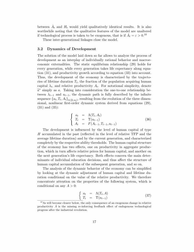
3.2 Dynamics of Development

The solution of the model laid down so far allows to analyze the process ofdevelopment as an interplay of individually rational behavior and macroe-conomic externalities. The static equilibrium relationship (29) holds forevery generation, while every generation takes life expectancy along equa-tion (31), and productivity growth according to equation (33) into account.Thus, the development of the economy is characterized by the trajecto-ries of lifetime duration Tt, the fraction of the population acquiring humancapital λt, and relative productivity At. For notational simplicity, denotea∗ simply as a. Taking into consideration the one-to-one relationship be-tween λt−1 and at−1, the dynamic path is fully described by the infinitesequence at, Tt, Att∈[0,∞), resulting from the evolution of the three dimen-sional, nonlinear first-order dynamic system derived from equations (29),(31) and (35):

at = Λ(Tt, At)Tt = Υ(at−1)At = F (At−1, Tt−1, at−1)

(36)

The development is influenced by the level of human capital of typeH accumulated in the past (reflected in the level of relative TFP and theaverage lifetime duration) and by the current generation, and characterizedcompletely by the respective ability thresholds. The human capital structureof the economy has two effects, one on productivity in aggregate produc-tion, which in turn affects relative prices for human capital, and another onthe next generation’s life expectancy. Both effects concern the main deter-minants of individual education decisions, and thus affect the structure ofhuman capital accumulation of the subsequent generation, and so on.

The analysis of the dynamic behavior of the economy can be simplifiedby looking at the dynamic adjustment of human capital and lifetime du-ration conditional on the value of the relative productivity. We thereforeconcentrate attention on the properties of the following system, which isconditional on any A > 0:

at = Λ(Tt, A)Tt = Υ(at−1)

(37)

10As will become clearer below, the only consequence of an exogenous change in relativeproductivity A is the missing re-inforcing feedback effect of endogenous technologicalprogress after the industrial revolution.

17

This system delivers the dynamics of human capital formation and life ex-pectancy for any given level of technology. From the previous discussionwe know that the first equation of the conditional system is defined forat ∈ (at (A) , 1] and T ∈ [e,∞) .

In what follows, we denote the S-shaped locus Tt = Λ−1(at, A) in thespace T, a, which results from the individual decision problem, by HH (A),and the locus Tt = Υ(at−1) representing the intergenerational externalityon lifetime duration by TT . Any steady state of the conditional system ischaracterized by the intersection of the two loci HH (A ) and TT :

Definition 2. A dynamic equilibrium of the conditional system given by(37) is a vector

aC , TC

with aC ∈ (a (A) , 1] and TC ∈ [e,∞), which

constitutes a steady state solution for the dynamic system (37) such that,for any A ∈ (0,∞):

aC = Λ(TC , A)TC = Υ(aC)

We are now in a position to characterize the set of steady states of theconditional system:

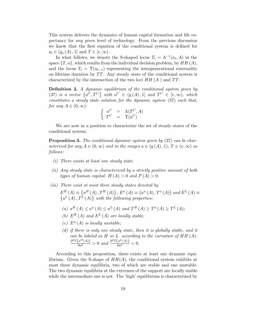
Proposition 3. The conditional dynamic system given by (37) can be char-acterized for any A ∈ (0,∞) and in the ranges a ∈ (a (A) , 1), T ∈ (e,∞) asfollows:

(i) There exists at least one steady state.

(ii) Any steady state is characterized by a strictly positive amount of bothtypes of human capital: H (A) > 0 and P (A) > 0.

(iii) There exist at most three steady states denoted by

EH (A) ≡aH (A) , TH (A)

, Eu (A) ≡ au (A) , T u (A) and EL (A) ≡

aL (A) , TL (A)

with the following properties:

(a) aH (A) ≤ au (A) ≤ aL (A) and TH (A) ≥ T u (A) ≥ TL (A);

(b) EH (A) and EL (A) are locally stable;

(c) Eu (A) is locally unstable;

(d) if there is only one steady state, then it is globally stable, and itcan be labeled as H or L according to the curvature of HH (A):∂2T(aH(A))

∂a2 > 0 and∂2T(aL(A))

∂a2 < 0.

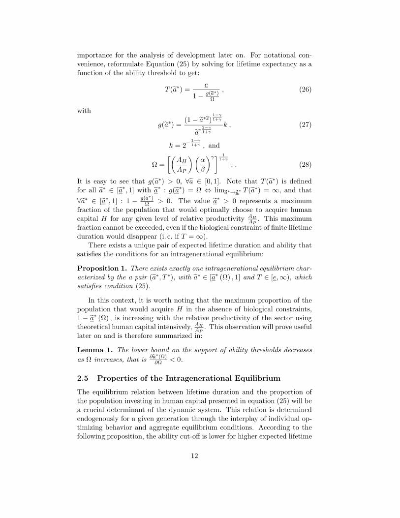
According to this proposition, there exists at least one dynamic equi-librium. Given the S-shape of HH(A), the conditional system exhibits atmost three dynamic equilibria, two of which are stable and one unstable.The two dynamic equilibria at the extremes of the support are locally stablewhile the intermediate one is not. The ’high’ equilibrium is characterized by

18

a relatively large fraction of the population acquiring H and large lifetimeexpectancy, and the locus HH (A) is locally convex in aH

t . The ’low’ equi-librium is characterized by low lifetime duration and correspondingly a littleshare of the population acquiring H. The locus HH (A) is locally concavein aL.

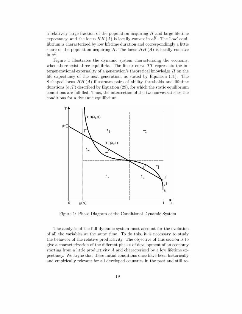
Figure 1 illustrates the dynamic system characterizing the economy,when there exist three equilibria. The linear curve TT represents the in-tergenerational externality of a generation’s theoretical knowledge H on thelife expectancy of the next generation, as stated by Equation (31). TheS-shaped locus HH (A) illustrates pairs of ability thresholds and lifetimedurations (a, T ) described by Equation (29), for which the static equilibriumconditions are fulfilled. Thus, the intersection of the two curves satisfies theconditions for a dynamic equilibrium.

T

HH(at,A)

ρ+T

TT(at-1)

T

e

0 a (A) 1 a

Figure 1: Phase Diagram of the Conditional Dynamic System

The analysis of the full dynamic system must account for the evolutionof all the variables at the same time. To do this, it is necessary to studythe behavior of the relative productivity. The objective of this section is togive a characterization of the different phases of development of an economystarting from a little productivity A and characterized by a low lifetime ex-pectancy. We argue that these initial conditions once have been historicallyand empirically relevant for all developed countries in the past and still re-

19

main so in most of the underdeveloped countries today. To this end it issufficient to concentrate attention to the main characteristics of the dynamicevolution of A, while there is no need to characterize its path in detail.

We begin the analysis of development by looking at productivity changesover the course of generations. Human capital H helps in adopting new ideasand technologies, and thus creates higher productivity gains than practicalhuman capital P . This means that in the long run relative productivity At

will tend to increase, which in turn tends to reinforce the role of theoreticalhuman capital H. This result is summarized by the following lemma:

Lemma 2. Relative Productivity At increases monotonically over time withlimt−→∞ At = +∞.

Therefore, productivity increases faster in the sector using theoreticalhuman capital H more intensively, so that this sector becomes relativelymore productive over time. As a consequence, H becomes more attractiveto acquire. Note that the strict monotonicity of At over time depends onthe assumption AP.t = 0. However, this assumption is not necessary for themain argument. What is crucial is that relative productivity will eventuallybe increasing once a sufficiently large fraction of the population acquires H.In the simulations below, we allow AP.t > 0 starting from large AP.0 andsmall AH.0. Relative productivity At is, in that case, initially decreasing,reflecting the larger innovative dynamics of sector P in during early stagesof development, but since H is relative more important than P for techno-logical progress in any sector in the long run, AH leapfrogs AP . Therefore,At is eventually increasing and keeps increasing from this point on. Thequalitative prediction is totally unchanged, with the only difference that inearly stages of development the high productivity in the P sector reinforcesthe tendency to acquire P and, in this way, delays massive human capitalacquisition even further.

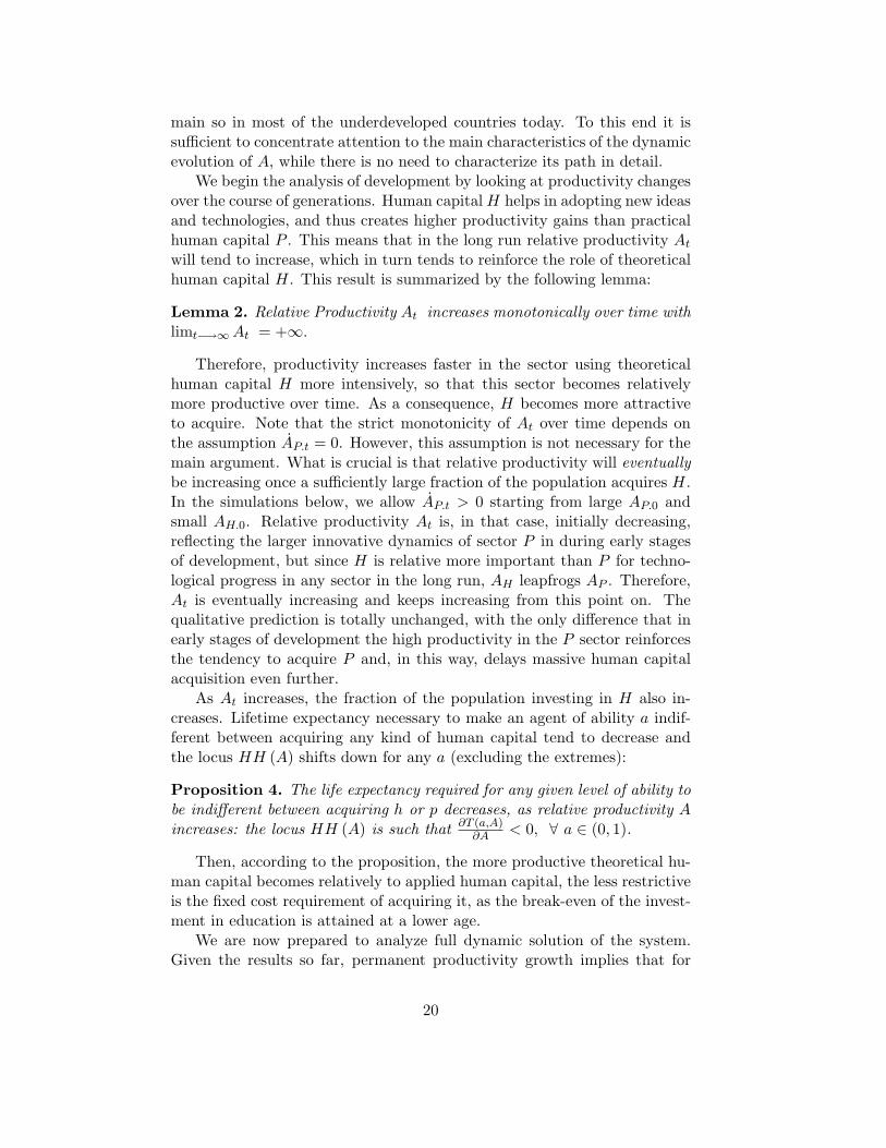
As At increases, the fraction of the population investing in H also in-creases. Lifetime expectancy necessary to make an agent of ability a indif-ferent between acquiring any kind of human capital tend to decrease andthe locus HH (A) shifts down for any a (excluding the extremes):

Proposition 4. The life expectancy required for any given level of ability tobe indifferent between acquiring h or p decreases, as relative productivity Aincreases: the locus HH (A) is such that ∂T (a,A)

∂A < 0, ∀ a ∈ (0, 1).

Then, according to the proposition, the more productive theoretical hu-man capital becomes relatively to applied human capital, the less restrictiveis the fixed cost requirement of acquiring it, as the break-even of the invest-ment in education is attained at a lower age.

We are now prepared to analyze full dynamic solution of the system.Given the results so far, permanent productivity growth implies that for

20

a given life expectancy the ability threshold for becoming theoretically ed-ucated decreases, inducing a higher fraction of the population to acquiretheoretical human capital. Of course, this has feedback effects through theexternalities of this increase of the aggregate stock of theoretical knowledgein the economy on life expectancy and productivity of the subsequent gen-eration.

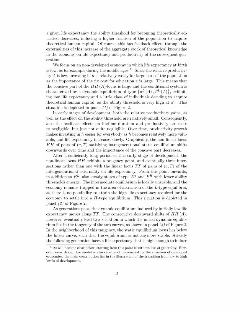
We focus on an non-developed economy in which life expectancy at birthis low, as for example during the middle ages.11 Since the relative productiv-ity A is low, investing in h is relatively costly for large part of the populationas the importance of the fix cost for education e is large. This means thatthe concave part of the HH (A)-locus is large and the conditional system ischaracterized by a dynamic equilibrium of type

aL (A) , TL (A)

, exhibit-

ing low life expectancy and a little class of individuals deciding to acquiretheoretical human capital, as the ability threshold is very high at aL. Thissituation is depicted in panel (1) of Figure 2.

In early stages of development, both the relative productivity gains, aswell as the effect on the ability threshold are relatively small. Consequently,also the feedback effects on lifetime duration and productivity are closeto negligible, but just not quite negligible. Over time, productivity growthmakes investing in h easier for everybody as h becomes relatively more valu-able, and life expectancy increases slowly. Graphically, the non-linear locusHH of pairs of (a, T ) satisfying intragenerational static equilibrium shiftsdownwards over time and the importance of the concave part decreases.

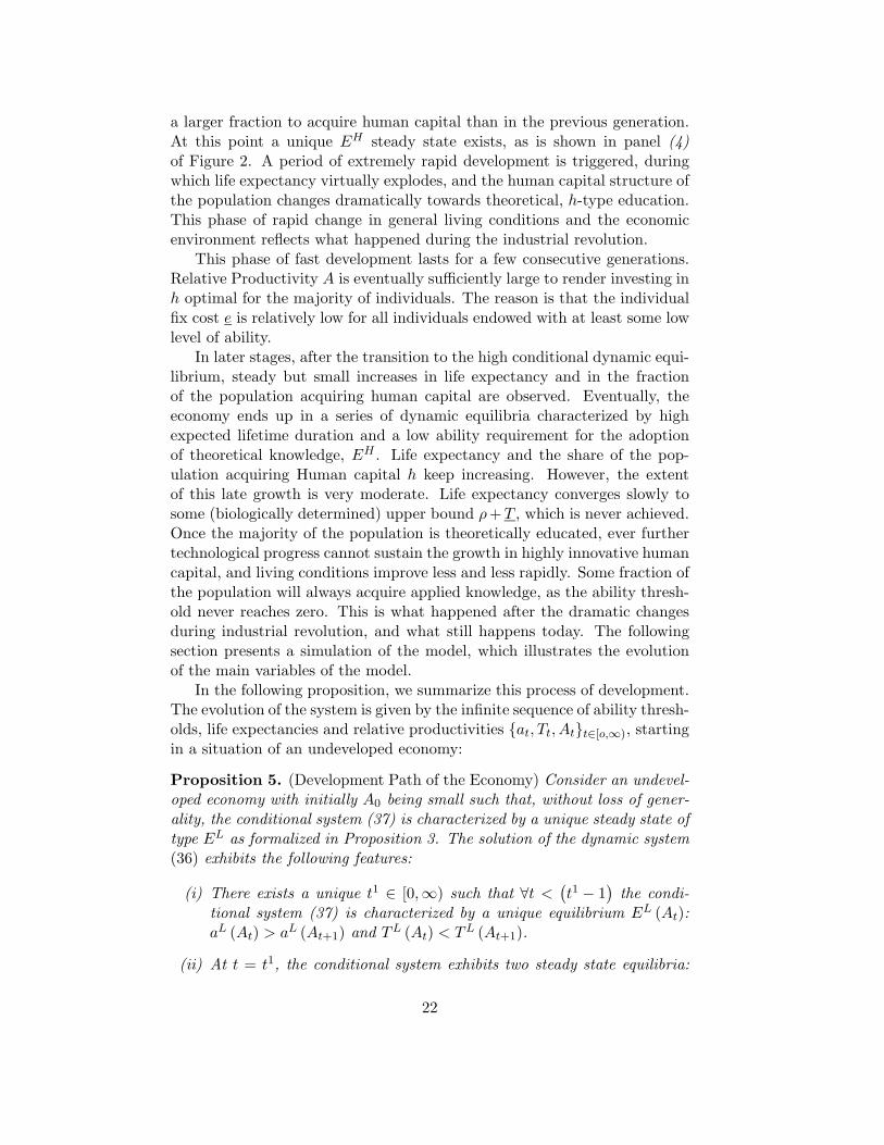
After a sufficiently long period of this early stage of development, thenon-linear locus HH exhibits a tangency point, and eventually three inter-sections rather than one with the linear locus TT of pairs of (a, T ) of theintergenerational externality on life expectancy. From this point onwards,in addition to EL, also steady states of type Eu and EH with lower abilitythresholds emerge. The intermediate equilibrium is locally unstable, and theeconomy remains trapped in the area of attraction of the L-type equilibria,as there is no possibility to attain the high life expectancy required for theeconomy to settle into a H-type equilibrium. This situation is depicted inpanel (2) of Figure 2.

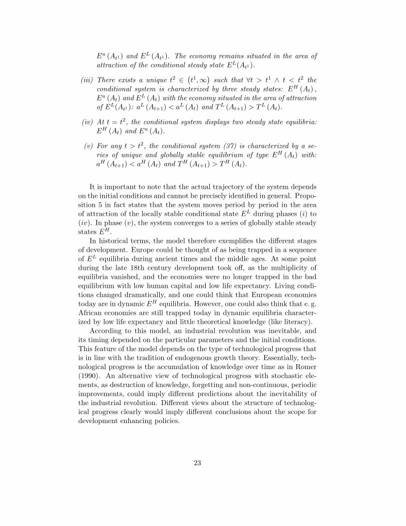
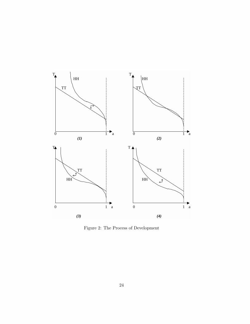
As generations pass, the dynamic equilibrium induced by initially low lifeexpectancy moves along TT . The consecutive downward shifts of HH (A),however, eventually lead to a situation in which the initial dynamic equilib-rium lies in the tangency of the two curves, as shown in panel (3) of Figure 2.In the neighborhood of this tangency, the static equilibrium locus lies belowthe linear curve, such that the equilibrium is not anymore stable. Alreadythe following generation faces a life expectancy that is high enough to induce

11As will become clear below, starting from this point is without loss of generality. How-ever, even though the model is also capable of demonstrating the situation of developedeconomies, the main contribution lies in the illustration of the transition from low to highlevels of development.

21

a larger fraction to acquire human capital than in the previous generation.At this point a unique EH steady state exists, as is shown in panel (4)of Figure 2. A period of extremely rapid development is triggered, duringwhich life expectancy virtually explodes, and the human capital structure ofthe population changes dramatically towards theoretical, h-type education.This phase of rapid change in general living conditions and the economicenvironment reflects what happened during the industrial revolution.

This phase of fast development lasts for a few consecutive generations.Relative Productivity A is eventually sufficiently large to render investing inh optimal for the majority of individuals. The reason is that the individualfix cost e is relatively low for all individuals endowed with at least some lowlevel of ability.

In later stages, after the transition to the high conditional dynamic equi-librium, steady but small increases in life expectancy and in the fractionof the population acquiring human capital are observed. Eventually, theeconomy ends up in a series of dynamic equilibria characterized by highexpected lifetime duration and a low ability requirement for the adoptionof theoretical knowledge, EH . Life expectancy and the share of the pop-ulation acquiring Human capital h keep increasing. However, the extentof this late growth is very moderate. Life expectancy converges slowly tosome (biologically determined) upper bound ρ+T , which is never achieved.Once the majority of the population is theoretically educated, ever furthertechnological progress cannot sustain the growth in highly innovative humancapital, and living conditions improve less and less rapidly. Some fraction ofthe population will always acquire applied knowledge, as the ability thresh-old never reaches zero. This is what happened after the dramatic changesduring industrial revolution, and what still happens today. The followingsection presents a simulation of the model, which illustrates the evolutionof the main variables of the model.

In the following proposition, we summarize this process of development.The evolution of the system is given by the infinite sequence of ability thresh-olds, life expectancies and relative productivities at, Tt, Att∈[o,∞), startingin a situation of an undeveloped economy:

Proposition 5. (Development Path of the Economy) Consider an undevel-oped economy with initially A0 being small such that, without loss of gener-ality, the conditional system (37) is characterized by a unique steady state oftype EL as formalized in Proposition 3. The solution of the dynamic system(36) exhibits the following features:

(i) There exists a unique t1 ∈ [0,∞) such that ∀t <(t1 − 1

)the condi-

tional system (37) is characterized by a unique equilibrium EL (At):aL (At) > aL (At+1) and TL (At) < TL (At+1).

(ii) At t = t1, the conditional system exhibits two steady state equilibria:

22

Eu (At1) and EL (At1). The economy remains situated in the area ofattraction of the conditional steady state EL(At1).

(iii) There exists a unique t2 ∈(t1,∞

)such that ∀t > t1 ∧ t < t2 the

conditional system is characterized by three steady states: EH (At) ,Eu (At) and EL (At) with the economy situated in the area of attractionof EL(At1): aL (At+1) < aL (At) and TL (At+1) > TL (At).

(iv) At t = t2, the conditional system displays two steady state equilibria:EH (At) and Eu (At).

(v) For any t > t2, the conditional system (37) is characterized by a se-ries of unique and globally stable equilibrium of type EH (At) with:aH (At+1) < aH (At) and TH (At+1) > TH (At).

It is important to note that the actual trajectory of the system dependson the initial conditions and cannot be precisely identified in general. Propo-sition 5 in fact states that the system moves period by period in the areaof attraction of the locally stable conditional state EL during phases (i) to(iv). In phase (v), the system converges to a series of globally stable steadystates EH .

In historical terms, the model therefore exemplifies the different stagesof development. Europe could be thought of as being trapped in a sequenceof EL equilibria during ancient times and the middle ages. At some pointduring the late 18th century development took off, as the multiplicity ofequilibria vanished, and the economies were no longer trapped in the badequilibrium with low human capital and low life expectancy. Living condi-tions changed dramatically, and one could think that European economiestoday are in dynamic EH equilibria. However, one could also think that e. g.African economies are still trapped today in dynamic equilibria character-ized by low life expectancy and little theoretical knowledge (like literacy).

According to this model, an industrial revolution was inevitable, andits timing depended on the particular parameters and the initial conditions.This feature of the model depends on the type of technological progress thatis in line with the tradition of endogenous growth theory. Essentially, tech-nological progress is the accumulation of knowledge over time as in Romer(1990). An alternative view of technological progress with stochastic ele-ments, as destruction of knowledge, forgetting and non-continuous, periodicimprovements, could imply different predictions about the inevitability ofthe industrial revolution. Different views about the structure of technolog-ical progress clearly would imply different conclusions about the scope fordevelopment enhancing policies.

23

T THH HH

TT TT

0 1 a 0 1 a (1) (2)

T T

TT TT

HH HH

0 1 a 0 1 a

(3) (4)

Figure 2: The Process of Development

24

4 Some Applications and Extensions

This section presents a simulation of the model to illustrate its capabilityto replicate this phenomenon. We then also address some straightforwardextensions of the model.

4.1 A Simple Simulation of Development

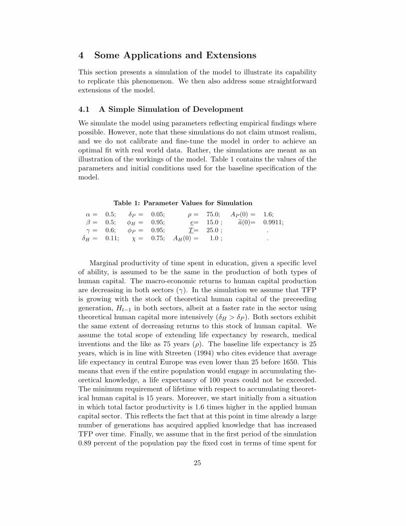
We simulate the model using parameters reflecting empirical findings wherepossible. However, note that these simulations do not claim utmost realism,and we do not calibrate and fine-tune the model in order to achieve anoptimal fit with real world data. Rather, the simulations are meant as anillustration of the workings of the model. Table 1 contains the values of theparameters and initial conditions used for the baseline specification of themodel.

Table 1: Parameter Values for Simulation

α = 0.5; δP = 0.05; ρ = 75.0; AP (0) = 1.6;β = 0.5; φH = 0.95; e= 15.0 ; a(0)= 0.9911;γ = 0.6; φP = 0.95; T= 25.0 ; .

δH = 0.11; χ = 0.75; AH(0) = 1.0 ; .

Marginal productivity of time spent in education, given a specific levelof ability, is assumed to be the same in the production of both types ofhuman capital. The macro-economic returns to human capital productionare decreasing in both sectors (γ). In the simulation we assume that TFPis growing with the stock of theoretical human capital of the preceedinggeneration, Ht−1 in both sectors, albeit at a faster rate in the sector usingtheoretical human capital more intensively (δH > δP ). Both sectors exhibitthe same extent of decreasing returns to this stock of human capital. Weassume the total scope of extending life expectancy by research, medicalinventions and the like as 75 years (ρ). The baseline life expectancy is 25years, which is in line with Streeten (1994) who cites evidence that averagelife expectancy in central Europe was even lower than 25 before 1650. Thismeans that even if the entire population would engage in accumulating the-oretical knowledge, a life expectancy of 100 years could not be exceeded.The minimum requirement of lifetime with respect to accumulating theoret-ical human capital is 15 years. Moreover, we start initially from a situationin which total factor productivity is 1.6 times higher in the applied humancapital sector. This reflects the fact that at this point in time already a largenumber of generations has acquired applied knowledge that has increasedTFP over time. Finally, we assume that in the first period of the simulation0.89 percent of the population pay the fixed cost in terms of time spent for

25

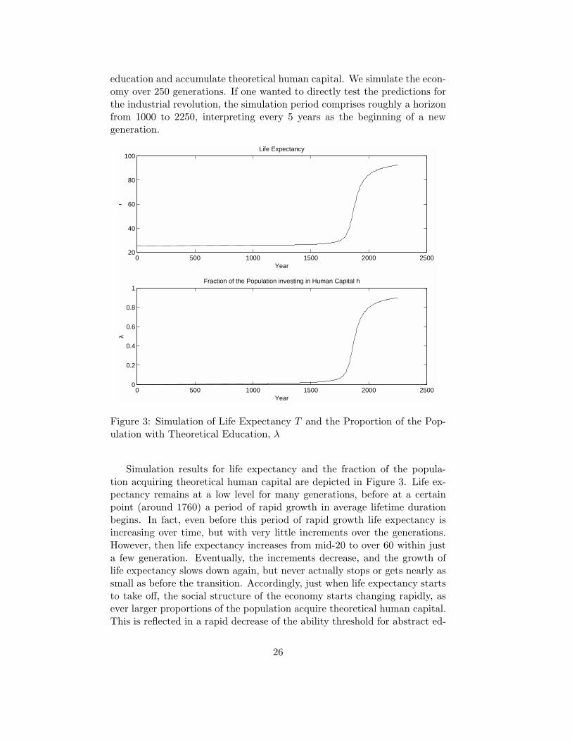
education and accumulate theoretical human capital. We simulate the econ-omy over 250 generations. If one wanted to directly test the predictions forthe industrial revolution, the simulation period comprises roughly a horizonfrom 1000 to 2250, interpreting every 5 years as the beginning of a newgeneration.

0 500 1000 1500 2000 250020

40

60

80

100Life Expectancy

Year

T

0 500 1000 1500 2000 25000

0.2

0.4

0.6

0.8

1Fraction of the Population investing in Human Capital h

Year

λ

Figure 3: Simulation of Life Expectancy T and the Proportion of the Pop-ulation with Theoretical Education, λ

Simulation results for life expectancy and the fraction of the popula-tion acquiring theoretical human capital are depicted in Figure 3. Life ex-pectancy remains at a low level for many generations, before at a certainpoint (around 1760) a period of rapid growth in average lifetime durationbegins. In fact, even before this period of rapid growth life expectancy isincreasing over time, but with very little increments over the generations.However, then life expectancy increases from mid-20 to over 60 within justa few generation. Eventually, the increments decrease, and the growth oflife expectancy slows down again, but never actually stops or gets nearly assmall as before the transition. Accordingly, just when life expectancy startsto take off, the social structure of the economy starts changing rapidly, asever larger proportions of the population acquire theoretical human capital.This is reflected in a rapid decrease of the ability threshold for abstract ed-

26

ucation. However, also this evolution slows down from its initial rapidness,as the share of educated people exceeds roughly three quarters of the popu-lation. When more than 90 percent accumulate theoretical knowledge, thisfraction hardly grows anymore. Nevertheless, due to the permanent growthin TFP, the aggregate stock of theoretical human capital keeps increasing,even after the transition, albeit at a somewhat slower rate.

0 500 1000 1500 2000 25000

200

400

600

800

1000Aggregate Income [..] and Productivity [-]

Year

A,Y

0 500 1000 1500 2000 25000

2

4

6

8Income Inequality

Year

I(90

/10)

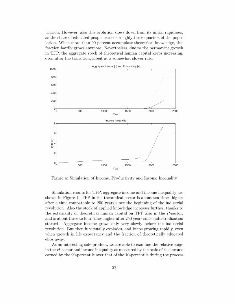
Figure 4: Simulation of Income, Productivity and Income Inequality

Simulation results for TFP, aggregate income and income inequality areshown in Figure 4. TFP in the theoretical sector is about ten times higherafter a time comparable to 250 years since the beginning of the industrialrevolution. Also the stock of applied knowledge increases further, thanks tothe externality of theoretical human capital on TFP also in the P -sector,and is about three to four times higher after 250 years since industrializationstarted. Aggregate income grows only very slowly before the industrialrevolution. But then it virtually explodes, and keeps growing rapidly, evenwhen growth in life expectancy and the fraction of theoretically educatedebbs away.

As an interesting side-product, we are able to examine the relative wagein the H-sector and income inequality as measured by the ratio of the incomeearned by the 90-percentile over that of the 10-percentile during the process

27

of development. The wage ratio initially decreases over what represents themiddle ages, as a consequence of learning in the applied sector. At the onsetof the industrialization there is even a slight dip in the relative wage, beforethe effects of increased human capital accumulation on life dependency andTFP fully come through and increase the relative value of theoretical humancapital very rapidly. The picture for inequality is similar. While it remainsroughly constant over a long period of time, the industrialization first leadsto a small decrease, before inequality starts increasing.

4.2 Empirical Relevance

Although the model presented above essentially describes a dynamic process,its implications can be tested using cross-sectional data of e. g. a group ofcountries. This requires the assumption that the underlying mechanisms arethe same across countries. The variation in the data is then interpreted asthe countries being at different levels of development.

Reis-Soares (2001) presents evidence from a sample of transitional coun-tries between 1960 and 1995. He finds a strong positive correlation betweenlife expectancy and average schooling levels, which can be seen as proxy oftheoretical human capital accumulation. Moreover, Soares computes cor-relations between per capita income and life expectancy at birth. For lowlevels of income and life expectancy, this relation is noticably positive, whileit becomes flatter and weaker the higher the level of per capita income.This is precisely the relation one would expect given the model presentedabove: Despite permanent income growth, the equilibrium lifetime durationgrows slower and slower during late stages of development. This result iscorroborated by the work of Swanson and Kopecky (1999) who run regres-sions explaining subsequent growth by current life expectancy for severalgroups of countries.12 Pooling all countries, the effect of life expectancyis highly significant and positive. However, when regressing separately fordifferent groups of countries, the effect is only highly significantly positivefor African and Asian countries, while close to zero and insignificant forboth Latin American and OECD countries. Interestingly, Africa and Asiaare also the groups of countries with the lowest average life duration (41.1and 51.5 years, respectively), suggesting that these groups of countries arestill involved in earlier stages of development where the lifetime durationconstraint is still stronger.

The predictions of the model correspond also with the findings of Lu-cas (2002), who argues that the industrial revolution was not the productof a succession of single events, but rather the outcome of continuous de-velopment even before the onset of rapid changes. However, while Lucasemphasizes fertility decisions as a potential explanation, we stress the role

12The data are for the period 1960 - 1985.

28

of life expectancy.By and large, it seems therefore that the main predictions of the model

are in line with empirical evidence.

4.3 Extensions

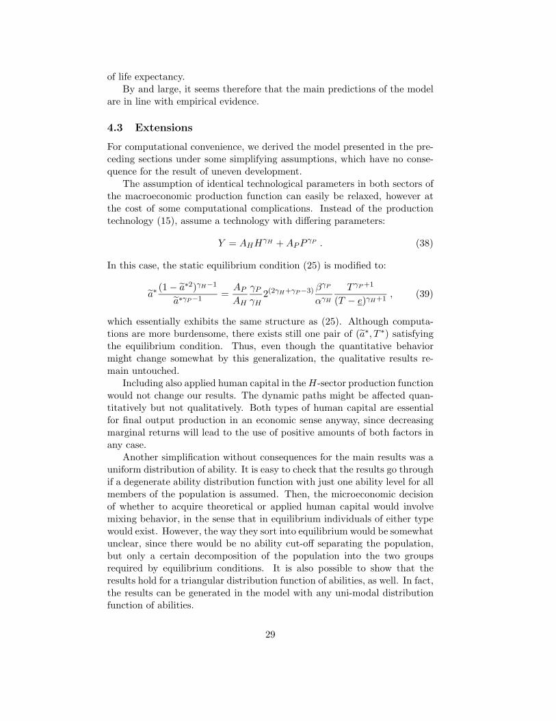
For computational convenience, we derived the model presented in the pre-ceding sections under some simplifying assumptions, which have no conse-quence for the result of uneven development.

The assumption of identical technological parameters in both sectors ofthe macroeconomic production function can easily be relaxed, however atthe cost of some computational complications. Instead of the productiontechnology (15), assume a technology with differing parameters:

Y = AHHγH + AP P γP . (38)

In this case, the static equilibrium condition (25) is modified to:

a∗(1 − a∗2)γH−1

a∗γP−1=

AP

AH

γP

γH2(2γH+γP−3) βγP

αγH

T γP +1

(T − e)γH+1, (39)

which essentially exhibits the same structure as (25). Although computa-tions are more burdensome, there exists still one pair of (a∗, T ∗) satisfyingthe equilibrium condition. Thus, even though the quantitative behaviormight change somewhat by this generalization, the qualitative results re-main untouched.

Including also applied human capital in the H-sector production functionwould not change our results. The dynamic paths might be affected quan-titatively but not qualitatively. Both types of human capital are essentialfor final output production in an economic sense anyway, since decreasingmarginal returns will lead to the use of positive amounts of both factors inany case.

Another simplification without consequences for the main results was auniform distribution of ability. It is easy to check that the results go throughif a degenerate ability distribution function with just one ability level for allmembers of the population is assumed. Then, the microeconomic decisionof whether to acquire theoretical or applied human capital would involvemixing behavior, in the sense that in equilibrium individuals of either typewould exist. However, the way they sort into equilibrium would be somewhatunclear, since there would be no ability cut-off separating the population,but only a certain decomposition of the population into the two groupsrequired by equilibrium conditions. It is also possible to show that theresults hold for a triangular distribution function of abilities, as well. In fact,the results can be generated in the model with any uni-modal distributionfunction of abilities.

29

Finally, all results carry over to a more realistic economy with overlap-ping generations. All assumptions about bequests and the determinants ofthe human capital investment decision, as well as the determinants of life ex-pectancy are maintained. Generations are born in fixed intervals.13 At thesame time, several generations can populate the economy. The number de-pends on the respective life expectancies the generations are endowed with.Human capital is interpreted as vintage human capital: it is characteristicfor a generation and cannot be substituted by the human capital of older oryounger generations. Therefore, every vintage of human capital is sold at itsown characteristic price. Hence, the decision how much time to invest in theacquisition of which type of human capital remains essentially the same asin the model presented in section 2. Productivity of a vintage, as well as lifeexpectancy of a generation are determined directly by the level of humancapital and productivity of the respective preceeding vintage. This vintageis not necessarily the parent generation. In a simulation of this overlappingframework, the frequency in which new generations are born is taken to befive years. Thus, children do not build on the knowledge of their parents,but on the knowledge of their immediately preceeding generation, whose inturn depends on that of older generations, etc.

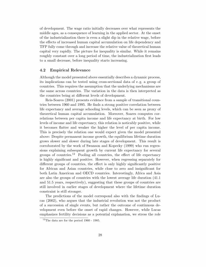
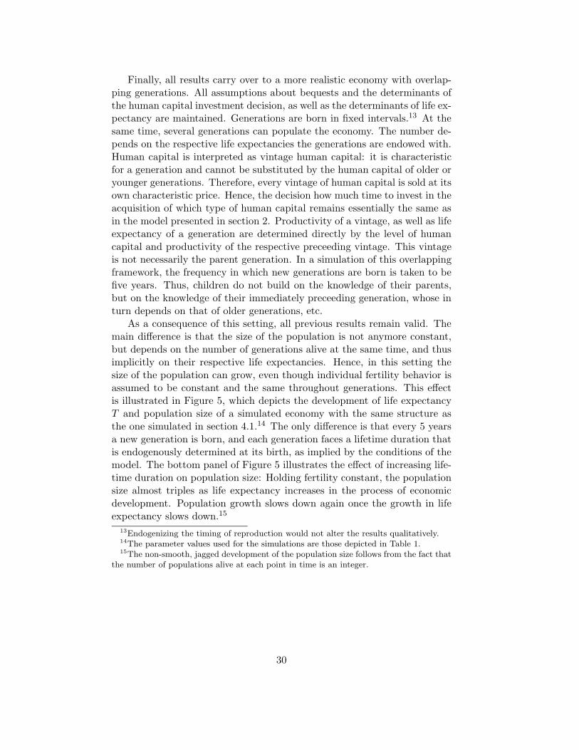
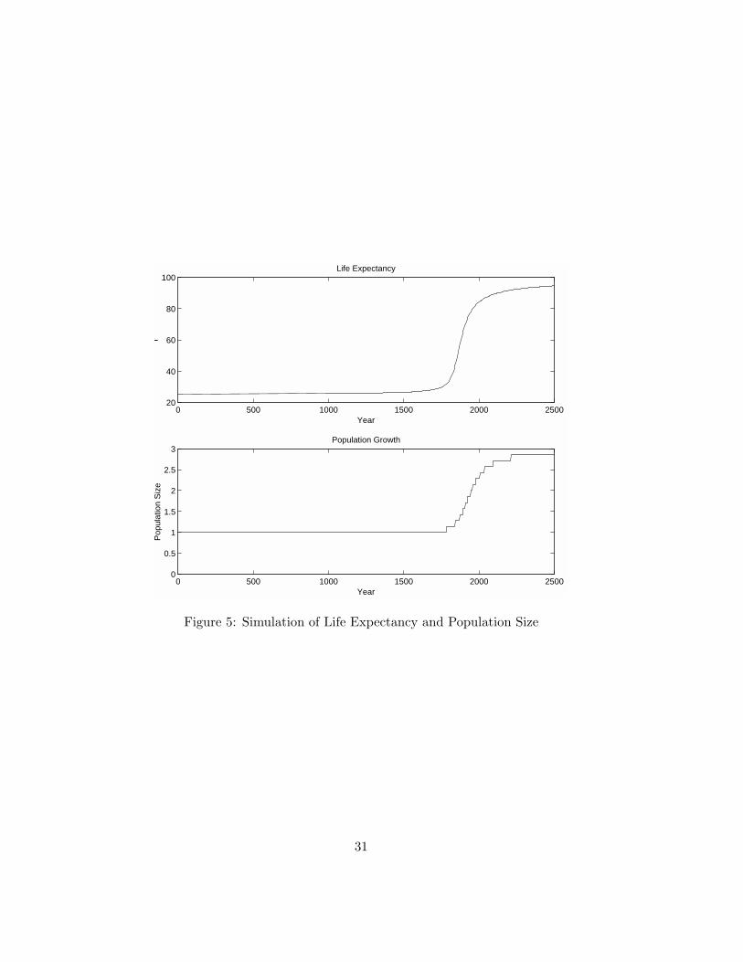
As a consequence of this setting, all previous results remain valid. Themain difference is that the size of the population is not anymore constant,but depends on the number of generations alive at the same time, and thusimplicitly on their respective life expectancies. Hence, in this setting thesize of the population can grow, even though individual fertility behavior isassumed to be constant and the same throughout generations. This effectis illustrated in Figure 5, which depicts the development of life expectancyT and population size of a simulated economy with the same structure asthe one simulated in section 4.1.14 The only difference is that every 5 yearsa new generation is born, and each generation faces a lifetime duration thatis endogenously determined at its birth, as implied by the conditions of themodel. The bottom panel of Figure 5 illustrates the effect of increasing life-time duration on population size: Holding fertility constant, the populationsize almost triples as life expectancy increases in the process of economicdevelopment. Population growth slows down again once the growth in lifeexpectancy slows down.15

13Endogenizing the timing of reproduction would not alter the results qualitatively.14The parameter values used for the simulations are those depicted in Table 1.15The non-smooth, jagged development of the population size follows from the fact that

the number of populations alive at each point in time is an integer.

30

0 500 1000 1500 2000 250020

40

60

80

100Life Expectancy

Year

T

0 500 1000 1500 2000 25000

0.5

1

1.5

2

2.5

3Population Growth

Year

Pop

ulat

ion

Siz

e

Figure 5: Simulation of Life Expectancy and Population Size

31

5 Concluding Remarks

One major puzzle, which economic explanations for the industrial revolu-tion have to address, is the apparently long stagnancy of economic condi-tions and life expectancy, which is suddenly followed by a period of fast anddramatic changes in both these dimensions. Previous contributions modelthe experience of the industrial revolution as the transition from a primi-tive, stagnant to a developed regime exhibiting permanent growth. Whateventually triggered this rapid transition is the topic of a lively discussionwithin the profession. This paper offers an explanation which is not basedon the existence of different regimes of the economy, but interprets long-term development including the experience of the industrial revolution asthe continuous evolution of the dynamic system of the economy.

This paper presents a microfoundation of human capital accumulationthat allows to explain patterns in long-term economic development. Themain contribution is that we explicitly take complex interactions betweeneconomic, social and biological factors into account, and model economicdevelopment and changes in life expectancy as endogenous processes. Animplication of this view is that even during the apparently stagnant envi-ronment before the industrial revolution, economic and biological factorsaffected each other. There is thus no need to explain a change in regimes,or a driving shock that triggered the transition. While there is evidence forboth, effects of life expectancy on human capital formation and technolog-ical progress, as well as economic conditions influencing life expectancy inlater stages of development, these interactions are difficult to identify at thevery beginning of the industrial revolution. In fact, the question of causalitymight never be settled, since from the empirical point of view its the detec-tion and the revelation of the precise timing of events is very problematic.This paper views these processes as being permanently interacted, alreadyduring periods of slow development.

The basic economic mechanism of the model remains unaltered through-out history. Life expectancy is the crucial state variable in the individualeducation decision. In turn, this education decision has implications for theeducation decision of future generations, both through life expectancy andproductivity changes. This means that advances in technological progress,human capital formation and lifetime duration reinforce each other. How-ever, the peculiarity of human capital is that every generation has to acquireit anew. But the costs for human capital formation are prohibitively highfor large parts of the population when the level of development is still lowand expected lifetime duration is short. However, at a certain point intime the entire system is sufficiently developed so that the positive feedbackloop has enough momentum to overcome the retarding effects of costs forhuman capital formation. The resulting development path exhibits an S-shape, with a long period of economic and biological stagnation, followed by

32

a relatively short period of dramatic change in living conditions and the eco-nomic and social environment. This setting implies that, given a standardview of endogenous technological progress, an industrial revolution eventu-ally was inevitable, its precise timing depending on the particular parameterconstellation. The mechanism presented in this paper is able to reproducethe observed patterns of long-term economic development without the needof relying on some exogenous events and strict temporal causalities. Bysimulating the model for illustration purposes, we show that the long-runbehavior of income, income growth, productivity, lifetime duration, popula-tion size and other key indicators of development implied by the model is inline with empirical evidence and stylized facts.

33

A Appendix

Proof of Proposition 1:

Proof. Consider Equation (26). For notational simplicity, denote a∗ simply as a, eas e. By standard calculus,

T ′(a) =e g′(a)

Ω[1 − g(a)

Ω

]2 < 0 , (40)

since g′(a) = − g(a)1+γ

[2−γ−γa2

2a2(1−a2)

]< 0, ∀a ∈ [0, 1]. Therefore, we conclude that for a

given set of parameters γ ∈ (0, 1), A = AH

AP, for every a ∈ [a, 1] there is one and

only one T > 0 such that (26) is satisfied.

Proof of Lemma 1:

Proof. The claim follows from the definition of a∗ (Ω), and the fact that g(a∗) isstrictly decreasing in a∗.

Proof of Proposition 2:The intuition of the proof proceeds as follows: We solve equilibrium condition

(25) for T as a function of a∗ and investigate the behavior of this function. Dueto the fact that T (a∗) is strictly monotonically decreasing within the admissiblesupport the function is invertible within this range of support. We then show thatthere exists one and only one a∗ for which the second derivative of this functionequals zero. Since the condition for the second derivative to equal zero cannotreadily be solved for a∗, we decompose it into two components and show that oneis strictly monotonically increasing within the support while the other is strictlymonotonically decreasing, such that there must exist one but only one a∗ for whichthe condition is satisfied by the intermediate value theorem. But if T (a) has asingle inflection point and is invertible, also a(T ) has a single inflection point andis therefore S-shaped.

Proof. Consider again Equation (26). We use the notational shorthands as in proofof Proposition 1. Using standard calculus, one can now show that:

T ′(a) =e g′(a)

Ω[1 − g(a)

Ω

]2 , (41)

and

T ′′(a) =e g′′(a)

Ω

[1 − g(a)

Ω

]+ 2e

[g′(a)]2Ω2[

1 − g(a)Ω

]3 . (42)

Due to the fact that T ′(a) < 0 ∀a ∈ [a, 1], we note that the function T (a) isinvertible in the range a ∈ [a, 1] of the support. Note also that T (a) ≥ T ∀a ∈ [0, 1],so the inverse function a(T ) is strictly monotonically decreasing for all positive T .

It will prove useful to substitute a2 with b and to re-write g(a) ≡ h(b) =(1−b)

1−γ1+γ

b2−γ

2(1+γ)k, g′(a) ≡ h′(b), and g′′(a) ≡ h′′(b), where b = (a)2. Thus define T (a) =

34

T (b), so the derivatives T ′(a) = T ′(b) and T ′′(a) = T ′′(b) can be re-written interms of b:

T ′(b) = − [T (b)]2

e

h′(b)Ω

Existence of an inflection point can already be inferred from a closer examination.Since

h′(b) = − k

2(1 + γ)(1 − b)

−2γ1+γ b

−11+γ (2 − γ − γb) = − k

1 + γh(b)B(b) < 0 ∀b ∈ [b, 1]

(where B(b) = 1−γ1−b

2−γ2b ), we know that also T ′(b) < 0 ∀b ∈ [b, 1]. Moreover, one

immediately sees that limb→1 h′(b) = −∞ ⇔ lima→1 T ′(a) = −∞, such that T hasinfinitely negative slope at both boundaries of the admissible support, suggestingthat there must exist at least one inflection point. From these arguments it isalso clear that the slope of the inverse function, a′(T ), converges to zero at bothboundaries of the support.

Analysis of the second derivative T ′′(b) allows to show existence and uniquenessof an inflection point. In particular, T ′′(b) = 0 requires:

h′′(b)(

1 − h(b)Ω

)= − 2

Ω(h′(b))2

⇔ kh(b)1 + γ

[B2(b)1 + γ

− B′(b)](

1 − h(b)Ω

)= − 2kh(b)

Ω(1 + γ)B2(b)

⇔(

−11 + γ

+B′(b)B2(b)

)=

2k

Ω(1 + γ)

(h(b)

1 − h(b)Ω

). (43)

(LHS ) = (RHS)

Noting thatB′(b)B2(b)

=−2γb2 + 4b(2 − γ) + 2(γ − 2)

(2 − γ − γb)2,

one finds that

∂(

B′(b)B2(b)

)∂b

=8(2 − γ)(1 − γ)(2 − γ − γb)3

> 0, ∀γ ∈ (0, 1), b ∈ [0, 1] .

This implies that the LHS of the condition for an inflection point (T ′′(b) = 0),equation (44), is strictly monotonically increasing in b. Furthermore, applyingcalculus one can also verify that the RHS of condition (44) is strictly monotonicallydecreasing in b on the support [0, 1]:

∂

(h(b)

1−h(b)Ω

)∂b

=h′(b)(

1 − h(b)Ω

)2 < 0, ∀b ∈ [b, 1] .

In order to ensure that there is a value of b for which (44) is satisfied, it remainsto be shown that the value of the LHS is smaller than that of the RHS for b = band larger for a = b = 1. Noting that LHS(b = 1) = −1

1+γ + 11−γ > 0 and that

RHS(b = 1) = 0 since h(1) = 0, one sees that the latter claim is true. The facts

35

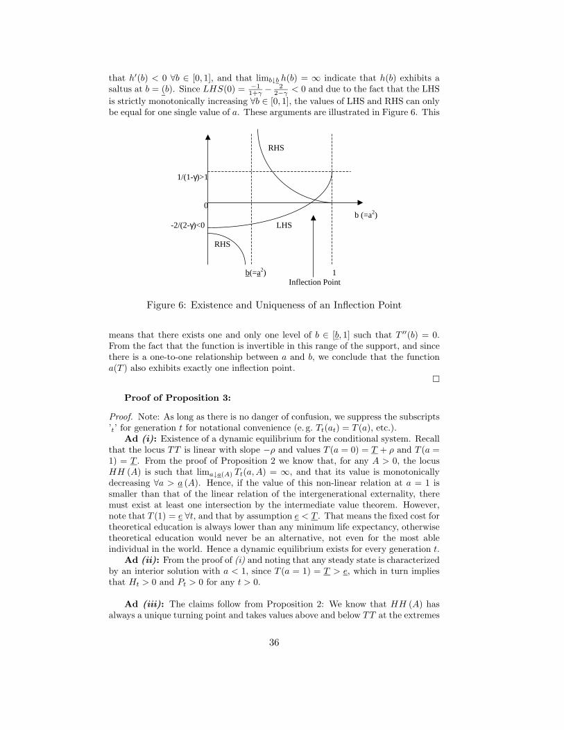
that h′(b) < 0 ∀b ∈ [0, 1], and that limb↓b h(b) = ∞ indicate that h(b) exhibits asaltus at b = (b). Since LHS(0) = −1

1+γ − 22−γ < 0 and due to the fact that the LHS

is strictly monotonically increasing ∀b ∈ [0, 1], the values of LHS and RHS can onlybe equal for one single value of a. These arguments are illustrated in Figure 6. This

RHS

1/(1-γ)>1

0 b (=a2)

-2/(2-γ)<0 LHS

RHS

b(=a2) 1 Inflection Point

Figure 6: Existence and Uniqueness of an Inflection Point

means that there exists one and only one level of b ∈ [b, 1] such that T ′′(b) = 0.From the fact that the function is invertible in this range of the support, and sincethere is a one-to-one relationship between a and b, we conclude that the functiona(T ) also exhibits exactly one inflection point.

Proof of Proposition 3:

Proof. Note: As long as there is no danger of confusion, we suppress the subscripts’t’ for generation t for notational convenience (e. g. Tt(at) = T (a), etc.).

Ad (i): Existence of a dynamic equilibrium for the conditional system. Recallthat the locus TT is linear with slope −ρ and values T (a = 0) = T + ρ and T (a =1) = T . From the proof of Proposition 2 we know that, for any A > 0, the locusHH (A) is such that lima↓a(A) Tt(a, A) = ∞, and that its value is monotonicallydecreasing ∀a > a (A). Hence, if the value of this non-linear relation at a = 1 issmaller than that of the linear relation of the intergenerational externality, theremust exist at least one intersection by the intermediate value theorem. However,note that T (1) = e ∀t, and that by assumption e < T . That means the fixed cost fortheoretical education is always lower than any minimum life expectancy, otherwisetheoretical education would never be an alternative, not even for the most ableindividual in the world. Hence a dynamic equilibrium exists for every generation t.

Ad (ii): From the proof of (i) and noting that any steady state is characterizedby an interior solution with a < 1, since T (a = 1) = T > e, which in turn impliesthat Ht > 0 and Pt > 0 for any t > 0.

Ad (iii): The claims follow from Proposition 2: We know that HH (A) hasalways a unique turning point and takes values above and below TT at the extremes

36

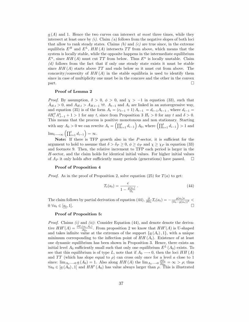
a (A) and 1. Hence the two curves can intersect at most three times, while theyintersect at least once by (i). Claim ( a) follows from the negative slopes of both locithat allow to rank steady states. Claims (b) and (c) are true since, in the extremeequilibria EH and EL, HH (A) intersects TT from above, which means that thesystem is locally stable, while the opposite happens in the intermediate equilibriumEu, since HH (A) must cut TT from below. Thus Eu is locally unstable. Claim(d) follows from the fact that if only one steady state exists it must be stablesince HH (A) starts above TT and ends below so it must cut from above. Theconcavity/convexity of HH (A) in the stable equilibria is used to identify themsince in case of multiplicity one must be in the concave and the other in the convexpart.

Proof of Lemma 2

Proof. By assumption, δ > 0, φ > 0, and χ > −1 in equation (33), such thatAH.t > 0, and AH.t > AH.t−1 ∀t. At−1 and At are linked in an autoregressive way,and equation (35) is of the form At = (ct−1 + 1) At−1 = dt−1At−1 , where dt−1 =δHφ

t Aχ.t−1 + 1 > 1 for any t, since from Proposition 3 Ht > 0 for any t and δ > 0.

This means that the process is positive monotonous and non stationary. Startingwith any A0 > 0 we can rewrite At =

(∏ti=1 di−1

)A0, where

(∏ti=1 di−1

)> 1 and

limt−→∞(∏t

i=1 di−1

)= ∞.

Note: If there is TFP growth also in the P -sector, it is sufficient for theargument to hold to assume that δ > δP ≥ 0, φ ≥ φP and χ ≥ χP in equation (33)and footnote 9. Then, the relative increment to TFP each period is larger in theH-sector, and the claim holds for identical initial values. For higher initial valuesof AP it only holds after sufficiently many periods (generations) have passed.

Proof of Proposition 4

Proof. As in the proof of Proposition 2, solve equation (25) for T (a) to get:

Tt(at) =e

1 − g(at)Ωt

. (44)

The claim follows by partial derivation of equation (44), ∂∂Ωt

Tt(at) = − g(at)e

(Ωt−g(at))2 <

0 ∀at ∈ [at, 1].

Proof of Proposition 5:

Proof. Claims (i) and (ii): Consider Equation (44), and denote denote the deriva-tive HH ′(A) = ∂Tt(at,At)

∂at. From proposition 2 we know that HH ′(A) is U-shaped

and takes infinite value at the extremes of the support a (At) , 1, with a uniqueminimum corresponding to the inflection point of HH (At). Existence of at leastone dynamic equilibrium has been shown in Proposition 3. Hence, there exists aninitial level A0 sufficiently small such that only one equilibrium EL (A0) exists. Tosee that this equilibrium is of type L, note that if A0 −→ 0, then the loci HH (A)and TT (which has slope equal to ρ) can cross only once for a level a close to 1since: limA0−→0 a (A0) = 1. Also along HH (A) the limA0−→0

∂T0∂a0

= ∞ > ρ; thus∀a0 ∈ [a (A0) , 1] and HH ′ (A0) has value always larger than ρ. This is illustrated

37

in Figure 7. Remember that δTt(at,At)δaAt

< 0 ∀at ∈ [a (At) , 1]. As time passes, rel-ative productivity At increases, as shown in Lemma 2. Hence, ∀t > 0 the locusHH (At) lies below the locus HH (A0) while the locus TT is unchanged. Bothcurves necessarily intersect for aL (At+1) < aL (At).

For illustrative purposes, continue with the Proof of Claim (v): The locusHH (A) becomes L-shaped as A gets large, and exhibits infinite value at a = 0 andvalue e elsewhere. The limA−→∞ T (a, A) = e, ∀a ∈ (0, 1]. Since a (∞) = 0, andT (a, A) = ∞ for any A, then T (0,∞) = ∞. This means that, eventually there willbe a unique equilibrium with aH

t close to zero. Existence of another equilibriumcan be ruled out by contradictions since it would imply that HH (At) > ρ forsome a < aH

t which is impossible due to the previous limits. Hence, from a certaingeneration onwards there exists a unique high type equilibrium EH .

|HH’| A

ρ

at1(ρ) at’

I at2(ρ) a

a(At) a(At’) a(At0)

Figure 7: Emergence of Multiple Equilibria

Proof of Claims (iii) and (iv): Obviously, the transition from a unique dynamicequilibrium EL to a unique dynamic equilibrium EH , the system must pass a phasecharacterized by multiple steady state equilibria. As generations pass we have from(41):

∂

∂Ωt

∣∣∣∣∂Tt(at, At)∂at

∣∣∣∣ =−Ωt + g(at) − 1(

1 − g(at)Ωt

)3

Ω3t

g′(at)e1Ωt

< 0 ∀at ∈ [at (At) , 1] . (45)

Also limA−→∞(

∂Tt(at,At)∂at

)= 0 ∀a = 1 and a = 0. Hence, as shown in Figure 7, the

locus HH ′ (A) shifts down monotonically. Its value eventually converges to zero inthe interior of the bounded support as A −→ ∞. From Proposition 2 we know thatthe locus HH ′ (A) has a unique minimum corresponding to the inflection point ofHH (A). Denote the ability threshold of the inflection point as aI

t for any t.Thus the full system passes from a series of unique equilibria EL, character-

ized by concavity of HH (A) to a series of unique equilibria EH , characterized byconvexity of HH (A). By continuity the dynamic equilibrium must, at the certain

38

point be characterized by the tangency between the two loci in the inflexion pointof HH (so that HH (A) is locally concave and convex).

Since as a consequence of Lemma 2 A grows monotonically and without boundas generations go by, and due to the resulting downward shift of HH ′ (A), there ex-

ists a t′ < ∞ such that: ∂Tt′ (aIt′ ,At′ )

∂at′= HH ′(at′ , At′) = ρ. For any t > t′ there exist

two levels of a: a1t (ρ) < aI

t < a2t (ρ) such that: ∂Tt(a

1t (ρ),At)∂at

= HH ′(a1t (ρ), At) =

∂Tt(a2t (ρ),At)∂at

= HH ′(a2t (ρ), At) = ρ. Hence, the locus HH (A) is convex in a1

t (ρ)

and concave in a2t (ρ) . Also, as the locus HH ′(a, A) shifts down, da1

t (ρ)dt < 0

and da2t (ρ)dt > 0 (see also Fig. 7). Finally, note that limA−→∞ a1

t (ρ) = 0 andlimA−→∞ a2

t (ρ) = 1 since HH ′(·,∞) takes value zero in the interior of the supportas shown previously.

By continuity, as the locus HH(a, A) shifts downward, there exists a t1 such

that:∂Tt′ (a

1t1 (ρ),At1 )

∂at′= HH ′(at1 , At1) = ρ and that HH(at1 , At1) = TT . At t1, a

new locally unstable steady state emerges in which a1t1 (ρ) = au

t1 , but the systemremains trapped in the locally stable low equilibrium. For any t > t1 the locusHH (A) shifts further downwards and exhibits three intersections with locus TT .Now define ∆(t) = a2

t (ρ) − aLt with ∆(t1) > 0. Now note that a2

t (ρ) < aLt for

any t > t′, and that ∂a2t (ρ)∂t > 0 and limA−→∞ a2

t (ρ) = 1. From the proof of Claims

(i) and (ii) above we know that ∂aLt

∂t < 0. Hence, ∂∆∂t < 0 and therefore there ∃

t2 > t1: ∆(t2) = 0 such that: a2t2 (ρ) = aL

t2 = aut2 .

During the life of generation t2 there exist only two dynamic steady state equi-libria with EL

t2 = Eut2 . For this generation, HH (at2 , At2) is tangent to TT so that

HH (at2 , At2) is both concave and convex in the equilibrium. However, due to con-dition (45), the static equilibrium locus HH keeps shifting down, and hence and∂a2

t (ρ)∂t < 0 also for t > t2. From this point onwards the concave part of HH (A)

lies entirely below TT , and only one dynamic equilibrium EH remains. For anyt > t2 the dynamic system converges, at a decreasing speed, to a sequence of EH

t

equilibria where aH (At+1) < aH (At) and TH (At+1) > TH (At) since the locusHH (at+1, At+1) lies always below the locus HH (at, At) while the locus TT re-mains unchanged. The dynamic equilibrium for t > t2 is characterized by muchlower levels of a and much higher levels of T than before t2. As a consequence, theadjustment involves rapid reductions in a and increases in T for a few generationsafter t2, but the growth rate eventually slows down as the system gets closer toEH .

Note: The dynamics of the full system necessarily follows the stages describedin the proposition and the actual path just depends on the initial value of A0.If A0 is large enough for the conditional system to display three steady states,then the convergence to one of the stable ones would depend just on the initialvalue of lifetime duration. If lifetime is large enough to bring the system to theEH equilibrium right from the beginning, then we are considering an economythat already escaped the low life expectancy equilibrium. Clearly the empiricallyrelevant initial conditions suggest to choose initial T0 in the area of attraction ofEL.

39

References

Becker, G. S., K. M. Murphy, and R. Tamura (1990): “Human Capi-tal, Fertility and Economic Growth,” Journal of Political Economy, 98(1),12–37.

Blackburn, K., and G. P. Cipriani (2002): “A Model of Longevity,Fertility and Growth,” Journal of Economic Dynamics and Control, 26,187–204.

Boucekkine, R., D. de la Croix, and O. Licandro (2002a): “VintageHuman Capital, Demographic Trends, and Endogenous Growth,” Journalof Economic Theory, 104(2), 340–375.

(2002b): “Early Mortality Declines at the Dawn of ModernGrowth,” mimeo, presented at Econometric Society European Meetings2002, Venice.

Croix, D. d. l., and O. Licandro (1999): “Life Expectancy and Endoge-nous Growth,” Economics Letters, 65, 255–263.

Easterlin, R. A. (2002): “Review of James C. Riley: ”Rising LifeExpectancy: A Global History”,” Economic History Services, URL:http://www.eh.net/bookreviews/library/0448.shtml(Feb. 12).

Galor, O., and O. Moav (2000): “Ability-Biased Technological Tran-sition and Economic Growth,” Quarterly Journal of Economics, CXV,469–497.

(2001): “Natural Selection and the Origin of Economic Growth,”CEPR Discussion Papers, 2727.

Galor, O., and D. N. Weil (2000): “Population, Technology, andGrowth: From Malthusian Stagnation to the Demographic Transition andBeyond,” American Economic Review, 90(4), 807–828.

Goodfriend, M., and J. McDermott (1995): “Early Development,”American Economic Review, 85(1), 116–133.

Hansen, G. D., and E. C. Prescott (1998): “Malthus to Solow,” NBERWorking Paper, 6858.

Jones, C. I. (2001): “Was an Industrial Revolution Inevitable? EconomicGrowth Over the Very Long Run,” mimeo.

(2002): “Sources of U.S. Economic Growth in a World of Ideas,”American Economic Review, 92(1), 220–239.

40

Kalemli-Ozcan, S. (2002): “Does Mortality Decline Promote EconomicGrowth?,” Journal of Economic Growth, forthcoming.

Kalemli-Ozcan, S., H. E. Ryder, and D. N. Weil (2000): “MortalityDecline, Human Capital Investment, and Economic Growth,” Journal ofDevelopment Economics, 62, 1–23.

Lichtenberg, F. R. (1998): “Pharmaceutical Innovation, Mortality Re-duction, and Economic Growth,” NBER Working Paper, 6569.

Lucas, R. E. (2002): Lectures on Economic Growth. Harvard UniversityPress, Cambridge, Massachusetts.

McKeown, T. (1977): The Modern Rise of Population. Butler and Tanner,London.

Mokyr, J. (1993): “Technological Progress and the Decline of EuropeanMortality,” American Economic Review, 83(2), 324–330.

Reis-Soares, R. (2001): “Life Expectancy, Educational Attainment, andFertility Choice,” mimeo.

Riley, J. C. (2001): Rising Life Expectancy: A Global History. CambridgeUniversity Press, New York.

Romer, P. M. (1990): “Endogenous Technological Change,” Journal ofPolitical Economy, 98(5), S71–S102.

Schultz, P. T. (1993): “Mortality Decline in the Low-Income World:Causes and Consequences,” American Economic Review, 83(2), 337–342.

Streeten, P. (1994): “Human Development: Means and Ends,” AmericanEconomic Review, 84(2), 232–237.

Swanson, C. E., and K. J. Kopecky (1999): “Lifespan and Output,”Economic Inquiry, 37(2), 213–225.

Vaupel, J. W. (1998): “Demographic Analysis of Aging and Longevity,”American Economic Review, 88(2), 242–247.

41

IZA Discussion Papers No.

Author(s) Title

Area Date

570 T. K. Bauer S. Bender

Technological Change, Organizational Change, and Job Turnover

1 09/02

571 O. Ashenfelter M. Greenstone

Using Mandated Speed Limits to Measure the Value of a Statistical Life

5 09/02

572 C. Y. Co I. N. Gang M.-S. Yun

Self-Employment and Wage Earning: Hungary During Transition

4 09/02

573 R. T. Riphahn O. Serfling

Item Non-Response on Income and Wealth Questions

6 09/02

574 R. Kuhn S. Stillman

Understanding Interhousehold Transfers in a Transition Economy: Evidence from Russia

4 09/02

575 H. Antecol D. A. Cobb-Clark S. J. Trejo

Human Capital and Earnings of Female Immigrants to Australia, Canada, and the United States

5 09/02

576 M. Fertig C. M. Schmidt H. Schneider

Active Labor Market Policy in Germany – Is There a Successful Policy Strategy?

6 09/02

577 K. Ariga G. Brunello

Are the More Educated Receiving More Training? Evidence from Thailand

2 09/02

578 I. N. Gang F. L. Rivera-Batiz M.-S. Yun

Economic Strain, Ethnic Concentration and Attitudes Towards Foreigners in the European Union

1 09/02

579 I. N. Gang M.-S. Yun

Decomposing Inequality Change in East Germany During Transition

4 09/02

580 I. N. Gang J. Landon-Lane M.-S. Yun

Gender Differences in German Upward Income Mobility

1 09/02

581 P. Cahuc F. Malherbet

Unemployment Compensation Finance and Labor Market Rigidity

5 09/02

582 P. Cahuc C. Gianella D. Goux A. Zylberberg

Equalizing Wage Differences and Bargaining Power: Evidence from a Panel of French Firms

6 09/02

583 P. Cahuc F. Fontaine

On the Efficiency of Job Search with Social Networks

5 09/02

584 C. J. Heinrich P. R. Mueser K. R. Troske

Welfare to Temporary Work: Implications for Labor Market Outcomes

3 09/02

585 M. Cervellati U. Sunde

Human Capital Formation, Life Expectancy and the Process of Economic Development

3 09/02

An updated list of IZA Discussion Papers is available on the center‘s homepage www.iza.org.