Highway Traffic Noise Prediction for Microcomputers: Modeling …onlinepubs.trb.org/Onlinepubs/trr/1988/1176/1176-006.pdf · TRANSPORTATION RESEARCH RECORD 1176 41 Highway Traffic

TRANSPORTATION RESEARCH RECORD 1176 41

Highway Traffic Noise Prediction for Microcomputers: Modeling of Ontario Simplified Program

F. W. JUNG AND C. T. BLANEY

Since its publication in 1977, the FWHA highway traffic noise prediction model, STAMINA, has been used in many manual and computerized forms. In this paper, a streamlined but somewhat limited version of the STAMINA model, written in BASIC for use on personal or pocket computers, is presented. The BASIC version can be used to predict noise from highway traffic for many simple situations. The program predicts noise from three standard classes of vehicle at one receiver location, shielded by a barrier of Infinite length. The model Includes the free field case and two parallel roadways, and it is consistent with the assumptions made In STAMINA 2.0. The modellng and underlying assumptions are explained in sufficient detail to contribute to a better understanding of the STAMINA 2.0 mainframe program and the mathematical modeling in gen­eral. For the applicable situations, the accuracy of computa­tion obtained is virtually the same as with STAMINA.

Several years ago, the method of traffic noise prediction best known as STAMINA was introduced in Ontario, Canada, as a computer program for mainframe computers. In a mainframe computer, the STAMINA program can handle complex cases of noise prediction. The underlying mathematical modeling for the program was first published as a manual method in a 1978 FHWA report (1). This document was the basis for several simplified methods designed for getting quick results in the course of planning activities. Among the new methods was a nomographic method developed by the Ontario Ministry of Transportation and Communications (MTC) (2).

STAMINA FOR PERSONAL COMPUTERS

The proliferation of personal computers renders all purely manual methods (including the one presented in original report) obsolete. However, the modeling technique presented in the FHWA report is still relevant and valid. It should be noted that the model is analytical, unlike other, earlier models. This means that the STAMINA model is, for example, flexible in changing noise emissions from vehicles.

Various attempts to simplify procedures and improve under­standing of the modeling behind the STAMINA program were published in 1981 (3). At that time, however, the technical community was not fully geared to using personal computers. Now that personal computers are almost ubiquitous, it is appropriate to present the simplified STAMINA modeling concepts in a form suitable for programming on microcomput-

Research and Development Branch, Ontario Ministry of Transporta­tion, Downsview, Ontario M3M US, Canada.

ers, leaving the mainframe programs for more complicated cases. The following concepts and improvements were de­veloped on the basis of the FHWA method (1, 3).

Modified Subtending Angle

The effect of ground absorption, estimated and expressed by a coeffj.cient, a, in free field segments, can be simply and fairly accurately incorporated by a modification of the subtending angles 1)>1 and c\>i· This downward modification of both angles narrows the field segment and thus compensates for the effect of ground absorption. In calculating a modified subtending angle, (j) = 1)>1' -1)>2', of a segment, the mathematical handling of the coefficient a becomes continuous and very simple (refer to the notation section).

Energy Level Equation

Instead of adding up (logarithmic) decibel values, an equation has been developed to use direct energy levels of (non­logarithmic) sound pressure energy. This not only assists in simplifying computations with a but also allows an additive treatment of vehicle traffic components. This procedure some­times saves separate calculations for cars and for medium and heavy trucks.

Curve Fitting of Basic Noise Attenuation Tables

The noise attenuation tables in Appendix B of the original FHWA report [(l), referred to hereinafter as Original STAMINA] have been curve-fitted for ll>R = 90 degrees and l)>L = -90 degrees, that is, for the infinitely long barrier (minimum values) and for the very short segments (maximum values). Interpolation expressions have been derived to take care of a large range of tabulated .1 values in Appendix B. Barrier segments, which are on one side of the receiver position and do not touch the receiver line perpendicular to the road axis, are not covered by the simplified method presented.

NOTATION

V = total traffic on the road or on the part of the highway being considered, in vehicles per hour.

42

p = fraction of car traffic (subscript A in Original STAMJNA); for instance, p = 0.85 means that cars represent 85 percent of V (P = 85).

q = fraction of medium truck traffic (originally, subscript MT).

r = fraction of heavy truck traffic (originally, subscript HT).

P, Q,R = percentage of car, medium truck, and heavy truck traffic, respectively.

s = average traffic speed, assumed to be uniform (km/hr).

Do = reference distance from centerline of traffic (D0 = 15 mis the standard value).

DN = horizontal distance from the noise source to the center of the nearest lane (m).

DF = horizontal distance from the noise source to the center of the farthest lane (m).

DE = equivalent lane distance, equal to .JDN DF, for free field only (m).

L = hourly reference energy emission level (dBA).

Leq equivalent sound level (dBA). ex. = ground cover coefficient, according to

Original STAMJNA (J): a = 0 for hard, reflective surfaces and ex. = 0.5 for soft, absorptive surfaces.

<I> = subtending segment angle in degrees, viewed from the point of the receiver toward the road.

<!>11 <1>2 = subtending angles for a segment (see Figure 1) (J).

<!>{. <!>2' = modified angles for a segment. $ = equivalent subtending angle ($ is reduced

because of soft ground cover, as discussed later in the paper).

Ll noise attenuation for a segment from a sound barrier parallel to the highway (dBA).

No = Fresnel number for path length difference B.

B = path length difference perpendicular to the road axis (see Figure 6).

I = sound barrier insertion loss (dBA).

p

ROADWAY

(·) (+)

p

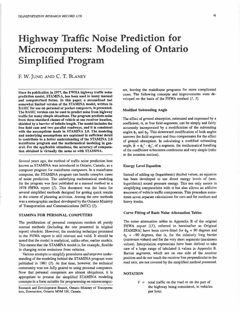
FIGURE 1 Subtending angle for "turning away" roadway.

TRANSPORTATION RESEARCH RECORD 1176

For free field conditions, ground cover coefficients can be estimated in accordance with the list in the following section.

GROUND COVER COEFFICIENTS, ex.

These values are proposed by the authors:

• ex. = 0 for reflective ground cover, such as paved parking lots, ice-covered ground, or collector and residential streets;

• a = 0.25 for moderately reflective ground cover, such as bare soil, niinor patches of grass, partially paved backyards, or parking lots interspersed with lawns;

• ex. = 0.5 for absorptive ground cover, such as lawns and soft soil fields or backyards with plants, flowers, and small shrubs; and

• ex. = 0.75 for very absorptive ground cover, such as backyards with trees and shrubs, cornfields, or similar surfaces.

MODIFIED SUBTENDING ANGLE

The concept can be easily recognized from Eliualion A-64 of Original STAMJNA (1, p. A-29). Looking from the receiver toward the roadway, the segment of investigation is enclosed by the angle <1>1 to the left and <1>z to the right, as shown in Figure 1 for a special case of a roadway that curves away. The angles enclose the subtending angle, <I>·

The subtending angle is always calculated as follows:

(1)

where <!i1 and <!i2 are measured from line P-P perpendicular to the road, at the receiver position R, positive in the clockwise direction. Note that the angle <!>1 in Figure 1 is negative.

In the case of soft, absorptive ground cover, the angles <!>1 and <!>2 should be modified, and a modified or equivalent subtending angle is calculated as follows:

(2)

The modified angles <l>i' and <1>2' have the same signs as the actual angles <!>1 and <!>2, respectively. The absolute values of <!>1 and <1>2 can be determined from Table 1, which is the solution of the following integral:

(3)

Substitution of Equation 3 into Equation 2 leads to Equation A-64 of Original STAMJNA, except for a factor of 180 degrees.

In the computer program, the angles <!>1, <1>2, <!>1', <!>2', and the rest are calculated from input values of distances and lengths of segments. In accordance with the convention for the sign of those angles, the lengths of segments, or parts thereof, can be positive (to the right) or negative (to the left; refer to Figures 1 and 2). For algebraic expressions of <!>' =/(ex.), refer to the section on curve fitting, later in this paper. Values for the

Jung and Blaney 43

p

p

XL , XR = Lett and right road distances, or visible road length

L 1 . L2 = Left and right barrier length

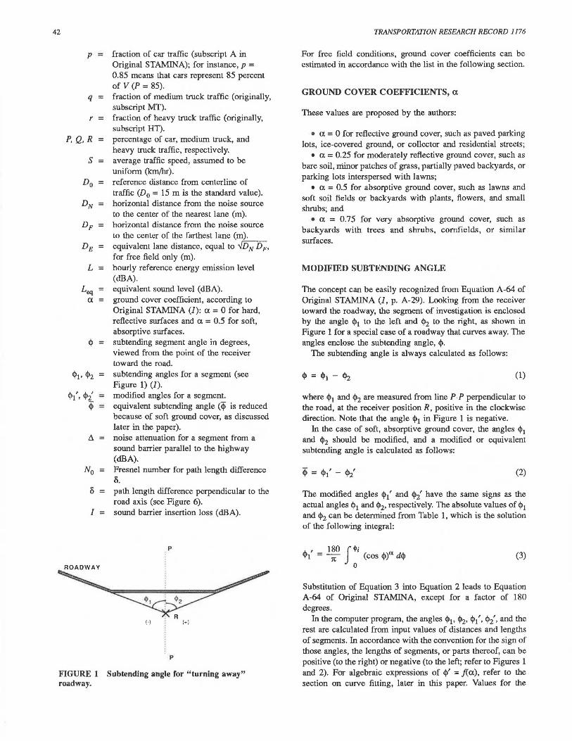
FIGURE 2 Subtending angles for barrier and roadway.

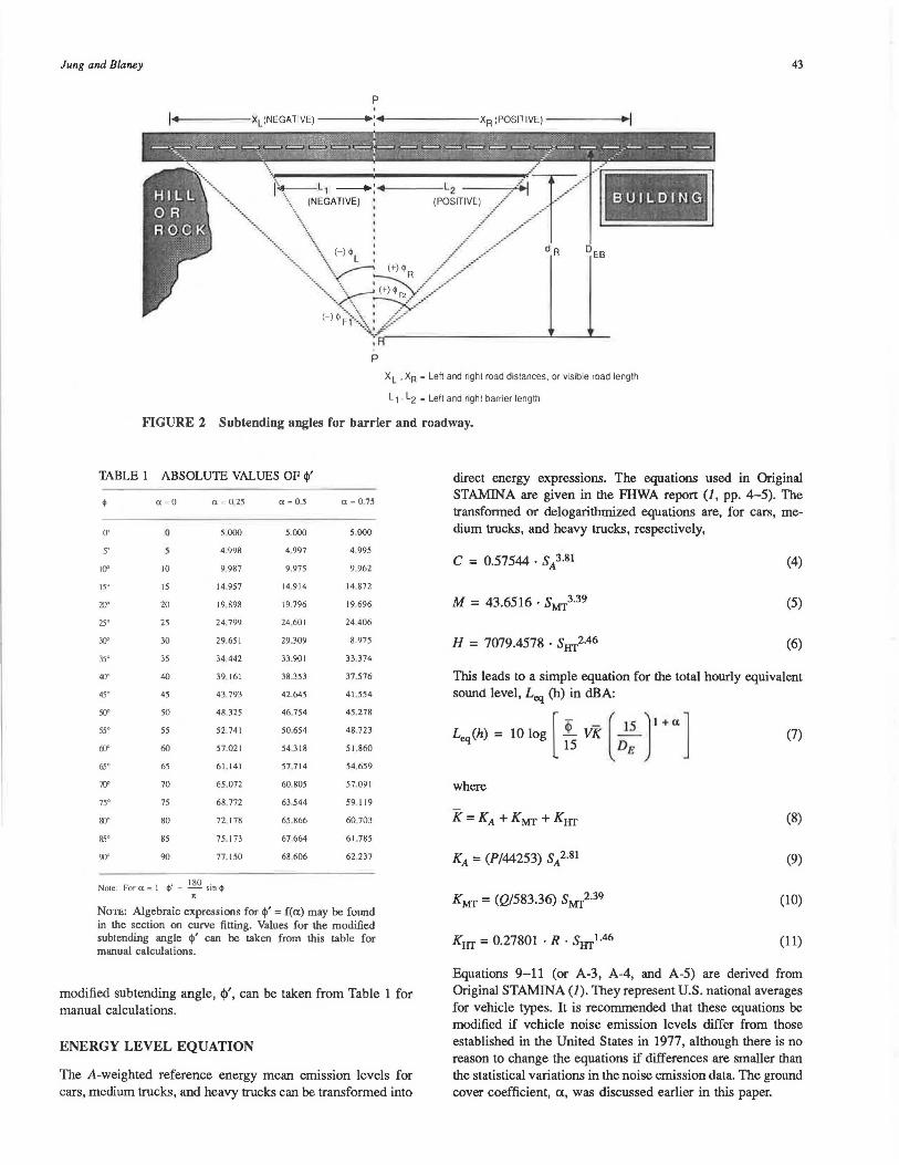
TABLE 1 ABSOLUTE VALUES OF ~'

<P a =0 a = O 25

(J' 0 5 .000

'f' s 4.998

I()" 10 9,987

15° 15 14 957

7fJ' 20 19 898

250 25 24, 799

]()" 30 29.651

35° 35 34.442

40" 40 39, 161

45° 45 43,793

YJ' 50 48,325

55° 55 52. 741

(fJ' 60 57.021

65' 65 61.141

7fl' 70 65,072

75° 75 68. 772

Ill" 80 72. 178

850 85 75. 173

'ff' 90 77. 150

Note: For o: = 1 <P' = .!!Q sin <P n

a= 0 5

5.000

4.997

9,975

14 914

19.796

24.601

29.309

33.901

38 .353

42.645

46 754

50,654

54 318

57.714

60 805

63 544

65 .866

67.664

68 .606

a= 0,75

5,000

4 995

9,962

14,872

19,696

24.406

8.975

33 ,374

37,576

41.554

45.278

48.723

51.860

54.659

57.091

59,119

60 703

61.785

62 237

NoTE: Algebraic expressions for cp' = f(a) may be fowid in the section on curve fitting. Values for the modified subtending angle cjl' can be taken from this table for manual calculations.

modified subtending angle, lj>', can be taken from Table 1 for manual calculations.

ENERGY LEVEL EQUATION

The A-weighted reference energy mean emission levels for cars, medium trucks, and heavy trucks can be transformed into

direct energy expressions. The equations used in Original STAMINA are given in the FHWA report (1, pp. 4-5). The transformed or delogarithmized equations are, for cars, me­dium trucks, and heavy trucks, respectively,

c = 0.57544 . SA3.81 (4)

M = 43.6516 · SMT3.39 (5)

H = 7079.4578 . Sm2.46 (6)

This leads to a simple equation for the total hourly equivalent sound level, Leq (h) in dBA:

L"l(h) = 10 log [ ~S vK [ ~: t •] (7)

where

(8)

KA = (P/44253) Si·Sl (9)

KMr = (Q/583.36) SMT2.39 (10)

Km = 0.27801 · R . Sml.46 (11)

Equations 9-11 (or A-3, A-4, and A-5) are derived from Original STAMINA (1) . They represent U.S. national averages for vehicle types. It is recommended that these equations be modified if vehicle noise emission levels differ from those established in the United States in 1977, although there is no reason to change the equations if differences are smaller than the statistical variations in the noise emission data. The ground cover coefficient, ex, was discussed earlier in this paper.

44

Data collected in Ontario during 1984 and 1985 resulted in a different set of equations:

KA= (P/1114.14) s;-041 (9')

KMr = (Q/8.2402) sMfi.406 (10')

KHT = 45.5051 · R · SHT0.259 (11')

These equations, labeled B-1, B-2, and B-3 in Original STAMINA, would replace original Equations A-3, A-4, and A-5 (9-11 in this paper). The underlying emission level equations can be found elsewhere (4).

CURVE FITTING OF TABLE 1 (EQUATION 3 RESULTS)

A closed solution of the integral expression of Equation 3 is not possible. Table 1 was established by nwnerical integration. The colwnns can be curve fitted approximately by the follow­ing equations (A-6 to A-9 in Original STAMINA). In this way, a solution that is suitable for small computers can be achieved, and calculations will be fast and direct.

<!> ·' = <!>· [ 1 - _M__ (ill) n l ' ' I <!>ii 90

M = (90) ( 0.58 a0.9 )

0.58 a.0·9 + 1

1 N = ~~~~~-0. 134 a + 0.225

For a= 1, the accurate solution is

;I; 180 ( . "'- . "' ) 't' = - Slil 'f'2 - Slil 't'l 1t

(12)

(13)

(14)

(15)

The special case of <!>i = 90 degrees and <!>1 = -90 degrees has been approximated by a different equation. For 0 :5; a :5; 0.75,

- 180 <1>=-----1+0.58 o.0·9

and for a = 1, the accurate solution in this case is

- 180 <1>=-1t/2

(16)

(17)

The ground cover coefficient is treated as a continuous vari­able. The approximation of the integral Equation 3, repre­sented by Equations 12-17, is accurate enough for all practical purposes.

BARRIER INSERTION

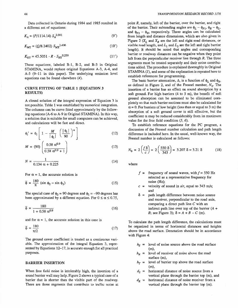
When free field noise is intolerably high, the insertion of a sound barrier wall may help. Figure 2 shows a typical case of a barrier that is shorter than the visible part of the roadway. There are three segments that contribute to traffic noise at

TRANSPORTATION RESEARCH RECORD 1176

point R, namely, left of the barrier, over the barrier, and right of the barrier. Their subtending angles are <l>L - <!>Fl• <l>R - <l>v and <l>n - <l>R• respectively. These angles can be calculated from length and distance dimensions, which are also given in Figure 2 (XL and XR are the left and right road distances, or visible road lc.:nglh, antl L1 and L2 are the left and right barrier length). It should be noted that angles and corresponding barrier or roadway distances can be negative when they point left from the perpendicular receiver line through R. The three segments must be treated separately and their noise contribu­tions added. The procedure is explained thoroughly in Original STAMINA (J), and some of the explanation is repeated here to establish references for programming.

The basic barrier attenuation, .'.\, is a function of <l>L and <l>R• as defined in Figure 2, and of the Fresnel number, N 0• The insertion of a barrier has an effect on sound absorption by a soft ground. For high barriers (4 to 5 m), the benefit of soft ground absorption can be assumed to be eliminated com­pletely so that such barrier sections must also be calculated for o. = 0. For barriers of low height (less than or equal to 3 m) the absorption of a soft ground cover is still effective, but the coefficient a may be reduced considerably from its maximum value for the free field condition (5, 6).

To establish reference equations for the PC program, a discussion of the Fresnel nwnber calculation and path length difference is included here. In the usual, well-known way, the Fresnel nwnber is calculated as follows:

(! 'O) ( 550 'O) N0 = 2 c = 2 343

= 3.207 'O "' 3.21 'O (18)

where

f = frequency of sound waves, withf = 550 Hz selected as a representative frequency for noise (Hz);

c = velocity of sound in air, equal to 343 mis; and

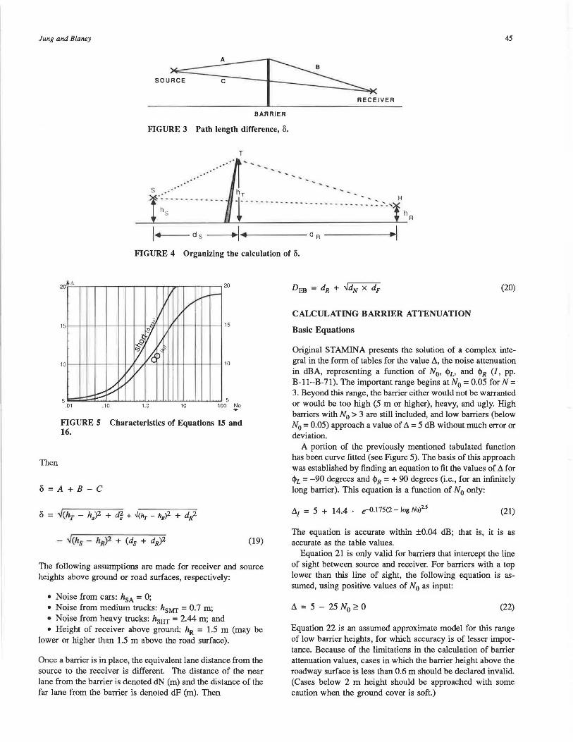
'O = path length difference between noise source and receiver, perpendicular to the road axis, comparing a direct path line C with an indirect path line over top of the barrier (A + B; see Figure 3); 'O = A + B - C (m).

To calculate the path length difference, the calculations must be organized in terms of horizontal distances and heights above the road surface. Denotation should be in accordance with Figure 4:

hs = level of noise source above the road surface (m),

hR = level of receiver of noise above the road surface (m),

hr = level of barrier top above the road surface (m),

ds = horizontal distance of noise source from a vertical plane through the barrier top (m), and

dR = horizontal distance of noise receiver from a vertical plane through the barrier top (m).

Jung and Blaney

BARRIER

FIGURE 3 Path length difference, 8.

T

' ' ' '

45

s

t-· ·· · ···· ·· ······ · · - - -~>: .• ., RhC

... -·~ - ..... - ..... _ ... ...

---~ dR •\

FIGURE 4 Organizing the calculation of 8.

Then

15

10

5 .01

v

~ /t.1 /

.........

.10

I/ ~ V ,;;

J r I

ll ~ ~ ~ ~' /

1.0

)

v .... -I

I

10

20

....-

15

10

5 100 No •

FIGURE 5 Characteristics of Equations 15 and 16.

o=A+B-C

(19)

The following assumptions are made for receiver and source heights above ground or road surfaces, respectively:

• Noise from cars: hsA = O; • Noise from medium trucks: hsMf = 0.7 m; • Noise from heavy trucks: hsIIT = 2.44 m; and • Height of receiver above ground: hR = 1.5 m (may be

lower or higher than 1.5 m above the road surface).

Once a barrier is in place, the equivalent lane distance from the source to the receiver is different. The distance of the near lane from the barrier is denoted dN (m) and the distance of the far lane from the barrier is denoted dF (m). Then

(20)

CALCULATING BARRIER ATTENUATION

Basic Equations

Original STAMINA presents the solution of a complex inte­gral in the form of tables for the value ~. the noise attenuation in dBA, representing a function of N0, <!>v and <l>R (1, pp. B-l l-B-71). The important range begins at N0 = 0.05 for N = 3. Beyond this range, the barrier either would not be warranted or would be too high (5 m or higher), heavy, and ugly. High barriers with N0 > 3 are still included, and low barriers (below N0 = 0.05) approach a value of !J. = 5 dB without much error or deviation.

A portion of the previously mentioned tabulated function has been curve fitted (see Figure 5). The basis of this approach was established by finding an equation to fit the values of~ for <l>L = -90 degrees and <l>R = + 90 degrees (i.e., for an infinitely long barrier). This equation is a function of N0 only:

!J,1

= 5 + 14.4 . e--0-175(2- log No)2.S (21)

The equation is accurate within ±0.04 dB; that is, it is as accurate as the table values.

Equation 21 is only valid for barriers that intercept the line of sight between source and receiver. For barriers with a top lower than this line of sight, the following equation is as­sumed, using positive values of N0 as input:

~ = 5 - 25 N0 ~ 0 (22)

Equation 22 is an assumed approximate model for this range of low barrier heights, for which accuracy is of lesser impor­tance. Because of the limitations in the calculation of barrier attenuation values, cases in which the barrier height above the roadway surface is less than 0.6 m should be declared invalid. (Cases below 2 m height should be approached with some caution when the ground cover is soft.)

46

The maximum values of .1. for short segments of barriers at the source-receiver line (J, pp. B-11-B-71) have also been curve fitted, as follows:

L\nax = 5.15 + 14.4 e--0.59(1 - log No)2 (23)

Between these .1. values, for infinitely long and very short barriers (.1.1 and L\nax), a complex interpolation formula has been derived, as follows:

(24)

where

(25)

rt = 1 + ( 1.25 + ~o ) [ 1 - 3.24 (1 tl>L ~ <l>n I J J (26)

This interpolation is valid for a certain limit of the difference between I <l>RI and I <l>LI , namely, for

<l>R + <l>L ~ 45 degrees (note: <l>L is negative) (27)

For differences outside this domain, <l>R + <l>L > 45 degrees, the following approximation is more accurate than Equations 25 and 26:

Tl = 1 + ( 1.25 + N; )

... ... <l>R 1 ... I > 1 ... I 'i'E = - 'i'L - S I 'f'L I I 'f'R I

(28)

(29)

,,.,£\\. ~JV)

Normally, <l>R is always positive and <l>L is always negative, according to definitions given in Figures 1 and 2 and earlier in the text. However, small angles of opposite sign (up to 10 degrees) can be accepted. Thus the following condition was introduced: if <l>R < -10 degrees or <l>L > + 10 degrees, the barrier insertion loss is declared invalid.

Ground Absorption

In the selection of a ground absorption coefficient, u, the following factors should be noted. When the ground cover coefficient Up for free field sound absorption is selected in accordance with the list presented in the earlier section on coefficient u, the program user should understand that the recommended values are only for normal, fairly even terrain. It should be noted that the beneficial effect of ground absorption (i.e., the coefficient u) deteriorates when the height of the sound propagation paths between source and receiver above the absorptive ground increases beyond the normal average height of source and receiver. This condition occurs with high noise barriers, but it also occurs also when the ground between source and receiver is significantly depressed.

TRANSPORTATION RESEARCH RECORD 1176

In the STAMINA 2.0 mainframe computer program the value uB (for barrier present) is therefore set to zero in any segment at which a barrier is present before the attenuation,~. is deducted (refer to the terms LB and .1. in Equation 26). Generally, this results in a much reduced or decreased net insertion loss (compared to /':,,). For very low barrier heights this could even lead to negative values for this net insertion loss, which would actually be an apparent gain in noise level above the free field condition level, in spite of the presence of a barrier. The program avoids such embarrassing contradic­tions by internal controls (IF LL < LF THEN LL = LF), without having a true solution.

When a valley or a ground depression of some kind is located between the source and receiver, the coefficient uF

should be selected accordingly, that is, below the pertinent value indicated in the list presented earlier. A further reduction from uF to uB is then less severe.

For barriers of low and moderate heights (below 3 m) there is a transition problem with the value Up and zero. Further guidance on this issue can be found in the work of Jung (6). Without this precaution, both the PC versions presented here and the mainframe STAMINA would underestimate the effect of low barriers in a terrain of absorptive ground. The problem of gr°ound absorption, however, has not yet been sufficiently clarified that a definite procedure can be recommended as a solution.

CALCULATION PROCEDURES

Calculations are carried out for the three vehicle types (cars, medium trucks, and heavy trucks) and for a maximum of two parallel roadways separately, and the results are then com­bined or added at a later stage. The program consists of one basic subroutine to calculate the free field noise for any segment, using dummy variables for DE, u, and <!>1 and <!>2 (the angles left and right of the segment, measured clockwise from the perpendicular line through point R, i.e., the line P-P in Figures 1 and 2). By using this subroutine, free field noise levels are calculated from the total roadway section (LF) from <!>Fl to <l>n, the barrier section (LB) from <l>L to <l>R• the segment left of the barrier (LX) from <!>Fl to <l>v and the segment right of the barrier (LY) from <l>R to <l>n (see Figure 2).

Another major part of the program consists of calculating barrier attenuation, denoted as .1., for each vehicle type and for the segment with barrier, from <l>L to <l>R• adjusted in accordance with the method shown above. The barrier net insertion loss (IL) for each vehicle type and roadway is then calculated as

IL = LF - (LB - .1. + LX + LY) (31)

where the terms in parentheses represent the noise level after barrier construction (LL).

At the end, the two kinds of noise levels, LF and LL, for each roadway are then added the LF and LL totals. A new, final net insertion loss is then calculated: I = LF - LL.

The sound absorption coefficient Up for ground cover, as listed earlier, is only valid for free field conditions (LF, LX, LY). The term LB must be calculated with a reduced u, and the STAMINA mainframe computer program assumes a value of uB = 0, which may be too low for very low barrier heights

Jung and Blalll!y

(6). To be consistent with STAMINA, the program here assumes that CJ.B = 0 unless another option is chosen.

PROGRAM COMPARISONS

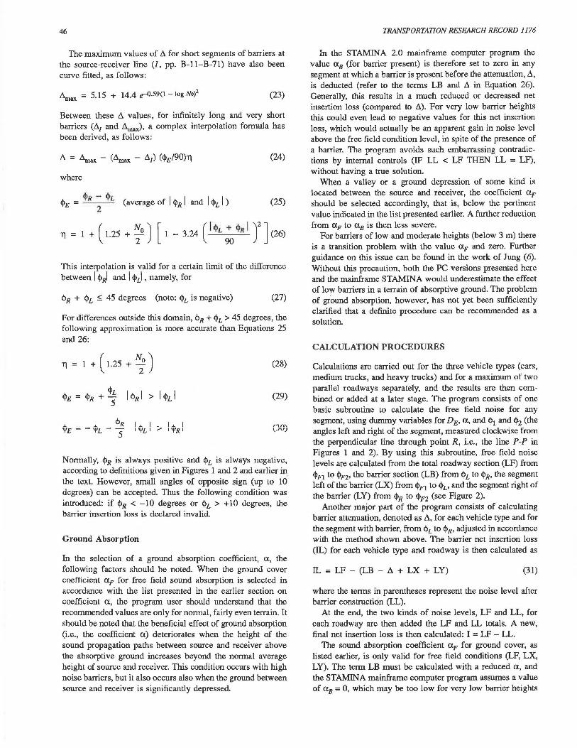
The proposed new program for microcomputers was compared with the mainframe STAMINA program. In most instances there were virtually no differences in the results. This was to be expected because the basic assumptions in modeling the programs were identical. However, inexplicable small dif­ferences of about 0.5 dBA were found at low barrier heights (less than or equal to 2.5 m) (see Figure 6).

dBA +PC 1 Mainframe

60 .0

59.0

58 . 0 1-.-.....-.~~-~~-.-1

1.4 2 3 4

Barrier Height

FIGURE 6 Comparison with the mainframe program STAMINA (variable barrier height).

BASIC PROGRAM

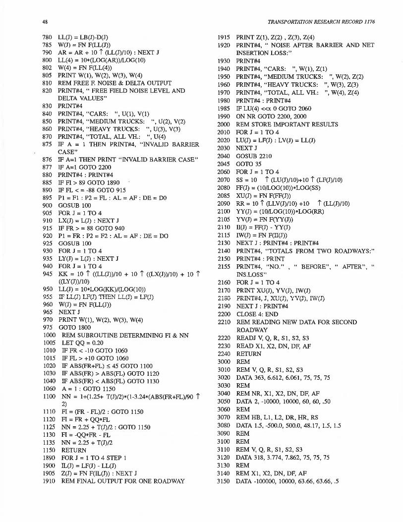
Program Listing

10 REM BARRIER NOISE PREDICTION PROGRAM 15 DTh1 LU(4), LV(4) : OPEN 4, 4, 0 20 READ V, Q, R, Sl, S2, S3 25 READ NR, Xl, X2, DN, DF, AF 30 LET P = 100-R-Q : DO= SQR(DN*DF) 40 LET PI= 3.14159265: X = 180/PI 45 Fl = X*ATN(Xl/DO) : F2 = X*ATN(X2/DO) 50 DI = DN-DR : D2 =DR-DR 55 DS = SQR(Dl*D2): DB= DR+ DS 60 FL= X*ATN(Ll/DR) : FR= X*ATN(L2/DR) 65 IF FL < Fl THEN FL = Fl 70 IF FR > F2 THEN FR = F2 75 DEF FN F(XX) = INT(IOOO*XX +.5)/1000 80 INPUT "ALPHA FOR BARRIER FIELD=" 85 GOTO 350 90 REM FREE FIELD NOISE SUBROUTINE 100 IF AL=O THEN PH=P2-Pl : GOTO 230 110 IF ALL=l THEN PH = (SIN(P2/X)-SIN(Pl/X)*X :

GOTO 230 130 N = l/(0.1334*AL + 0.225) 140 M = (90)*(0.58*AL i 0.9 + 1) 150 YI = ABS(Pl): Y2 = ABS(P2) 160 IF Pl = 0 THEN GOTO 180 170 PA= Pl*(l-(M/Yl)*(Yl/90.) i N) 180 IF P2 = 0 THEN GOTO 200

190 PB = P2*(l -(M/Y2)*(Y2/90.) i N) 200 IF Pl = 0 THEN LET PA = 0 210 IF P2 = 0 THEN LET PB = 0 220 PH = PB - PA 230 K(l) = (P/44253)*S 1 i 2.81 240 K(2) = (Q/583.36)*S2 i 2.39 250 K(3) = 0.2780l*R*S3 i l.46 260 K(4) = K(l) + K(2) + K(3) 270 FOR J = 1 TO 4 STEP 1 280 IF PH< 0.001 THEN L(J) = 0 290 IF PH< 0.001 GOTO 330 300 IF K(J) = 0 THEN L(J) = 0 310 IF K(J) = 0 GOTO 330

47

320 L(J) = (10/LOG(l0))*LOG((PH/15)*V*K(J)*(l5/DE) i (l+AL))

330 NEXT J 340 RETURN 350 REM FREE FIELD NOISE FOR C, MT, HT 360 Pl= Fl : P2 = F2: AL=AF: DE=DO 370 GOSUB 100 380 FOR J = 1 TO 4 STEP 1 390 LF(J) = L(J) 400 U(J) = FN F(LF(J)) 410 NEXT J 420 PRINT U(l), U(2), U(3), U(4) 440 IF A=l GOTO 810 450 REM FR. FIELD NOISE OF BARRIER SEC. 460 Pl= FL: P2 =AL= AB: DE= DB 470 GOSUB 100 480 FOR J = 1 TO 4 STEP 1 490 LB(J) = L(J) : NEXT J 500 REM CALCULATE DELTAS OF BARRIER 510 LET H(l) = 0.0 520 LET H(2) = 0.7 530 LET H(3) = 2.44 540 FOR J = 1 TO 3 STEP 1 550 AA = SQR((HB-H(J))*(HB-H(J)) + DS*DS) 560 BB = SQR((HB-HR)*(HB-HR + DR*DR) 570 CC= SQR ((H(J)-HR)*(H(J)-HR) + DB*DB) 580 PD(J) = AA + BB - CC 590 T(J) = 3.207*PD(J) (j()() NEXT J 610 GOSUB 1000 615 IF A = 1 GOTO 810 620 FOR J = 1 TO 3 STEP 1 630 LG= LOG(T(J))/LOG(lO) 640 DY= 5 + 14.4*EXP(-.175*(2-LG) i 2.5) 650 DX= 5.15 + 14.4*EXP(-.59*(1-LG i 2) 660 IF NN > 1.0 THEN NN = l 670 IF NN < 6.0 THEN NN = 6.0 720 D(J) = DX-(DX-D6)*(Fl/90) i NN 730 IF D(J) > 19.5 THEN D(J) = 19.5 740 IF HB-HR :5 (H(J) -HR)*(DR/DB) THEN D(J) = 5 -

25*T(J) 745 IF D(J) 0 THEN D(J) = 0 750 V(J) = FN F(D(J)) 755 NEXT J : AR = 0 760 PRINT V(l), V(2), V(3) 770 FOR J = 1 TO 3 STEP 1

48

780 LL(J) = LB(J)-D(J) 785 W(J) = FN F(LL(J)) 790 AR = AR + 10 i (LL(J)/10) : NEXT J 800 LL(4) = lO*(LOG(AR))/LOG(lO) 802 W(4) = FN F(LL(4)) 805 PRINT W(l), W(2), W(3), W(4) 810 REM FREE F. NOISE & DELTA OUTPUT 820 PRINT#4, " FREE FIELD NOISE LEVEL AND

DELTA VALUES" 830 PRINT#4 840 PRINT#4, "CARS: ", U(l), V(l) 850 PRINT#4, "MEDIUM TRUCKS: ", U(2), V(2) 860 PRINT#4, "HEAVY TRUCKS: ", U(3), V(3) 870 PRINT#4, "TOTAL, ALL VH.: ", U(4) 875 IF A = 1 THEN PRINT#4, "INVALID BARRIER

CASE" 876 IF A=l THEN PRINT "INVALID BARRIER CASE" 877 IF A= 1 GOTO 2200 880 PRINT#4 : PRINT#4 885 IF FI > 89 GOTO 1890 890 IF FL < = -88 GOTO 915 895 Pl = Fl : P2 = FL : AL = AF : DE = DO 900 GOSUB 100 905 FOR J = 1 TO 4 910 LX(J) = L(J) : NEXT J 915 IF FR>= 88 GOTO 940 920 Pl = FR : P2 = F2 : AL = AF : DE = DO 925 GOSUB 100 930 FOR J = 1 TO 4 935 LY(J) = L(J) : NEXT J 940 FOR J = 1 TO 4 945 KK = 10 i ((LL(J))/10 + 10 i ((LX(J))/10) + 10 i

((LY(J))/10) 950 LL(J) = lO*LOG(KK)/(LOG(lO))

960 W(J) = FN F(LL(J)) 965 NEXT J 970 PRINT W(l), W(2), W(3), W(4) 975 GOTO 1800 1000 REM SUBROUTINE DETERMJNING FI & NN 1005 LET QQ = 0.20 1010 IF FR< -10 GOTO 1060 1015 IF FL> +10 GOTO 1060 1020 IF ABS(FR+FL) ~ 45 GOTO 1100 1030 IF ABS(FR) > ABS(FL) GOTO 1120 1040 IF ABS(FR) < ABS(FL) GOTO 1130 1060 A = 1 : GOTO 1150 1100 NN = 1+(1.25+ T(J)/2)*(1-3.24*(ABS(FR+FL)/90 i

2) 1110 FI = (FR - FL)/2 : GOTO 1150 1120 FI =FR + QQ*FL 1125 NN = 2.25 + T(J)/2: GOTO 1150 1130 FI= -QQ•FR - FL 1135 NN = 2.25 + T(J)/2 1150 RETURN 1890 FOR J = 1 TO 4 STEP 1 1900 IL(J) = LF(J) - LL(J) 1905 Z(J) = FN F(IL(J)) : NEXT J 1910 REM FINAL OUTPUT FOR ONE ROADWAY

TRANSPORTATION RESEARCH RECORD 1176

1915 PRINT Z(l), Z(2) , Z(3), Z(4) 1920 PRINT#4, " NOISE AFTER BARRIER AND NET

INSERTION LOSS:" 1930 PRINT#4 1940 PRINT#4, "CARS: '', W(l), Z(l) 1950 PRINT#4, "MEDIUM TRUCKS: ", W(2), Z(2) 1960 PRINT#4, "HEAVY TRUCKS: ", W(3), Z(3) 1970 PRINT#4, "TOTAL, ALL VH.: ", W(4), Z(4) 1980 PRINT#4: PRINT#4 1985 IF LU(4) «x 0 GOTO 2060 1990 ON NR GOTO 2200, 2000 2000 REM STORE IMPORTANT RESULTS 2010 FOR J = 1 TO 4 2020 LU(J) = LF(J) : LV(J) = LL(J) 2030 NEXT J 2040 GOSUB 2210 2045 GOTO 35 2060 FOR J = 1 TO 4 2070 SS = 10 i (LU(J)/10)+10 i (LP(J)/10) 2080 FF(J) = (10/LOG(lO))*LOG(SS) 2085 XU(J) = FN F(FF(J)) 2090 RR= 10 i (LLV(J)/10) +10 i (LL(J)/10) 2100 YY(J) = (10/LOG(lO))*LOG(RR) 2105 YV(J) = FN F(YY(J)) 2110 II(J) = FF(J) - YY(J) 2115 IW(J) = FN F(II(J)) 2130 NEXT J: PRINT#4: PRINT#4 2140 PRINT#4, "TOTALS FROM TWO ROADWAYS:" 2150 PRINT#4: PRINT 2155 PRINT#4, "NO." , " BEFORE", " AFTER", "

INS.LOSS" 2160 FOR J = 1 TO 4 2170 PRINT XU(J), YV(J), IW(J)

2190 NEXT J : PRINT#4 2200 CLOSE 4: END 2210 REM READING NEW DATA FOR SECOND

ROADWAY 2220 READJ V, Q, R, Sl, S2, S3 2230 READ Xl, X2, DN, DF, AF 2240 RETURN 3000 REM 3010 REM V, Q, R, Sl, S2, S3 3020 DATA 363, 6.612, 6.061, 75, 75, 75 3030 REM 3040 REM NR, Xl, X2, DN, DF, AF 3050 DATA 2, -10000, 10000, 60, 60, .50 3060 REM 3070 REM HB, L1, L2, DR, HR, RS 3080 DATA 1.5, -500.0, 500.0, 48.17, 1.5, 1.5 3090 REM 3100 REM 3110 REM V, Q, R, Sl, S2, S3 3120 DATA 318, 3.774, 7.862, 75, 75, 75 3130 REM 3140 REM Xl, X2, DN, DF, AF 3150 DATA -100000, 10000, 63.66, 63.66, .5

Jung and Blaney

Appendix D of Original STAMINA provides an example with similar input, except that HB = 4.0 m, Ll = 17.532 m, and L2 = 132.346 m (1).

Notation: Input Terms

NR = Number of roadways: one (1) or two (2). Xl = Length of visible roadway to the left of the

perpendicular receiver line; must be a negative value when measured to the left of that line (exception: skew to the right) (m).

X2 = Length of visible roadway to the right of the perpendicular receiver line; must be a positive value when measured to the right of the line (exception: skew to the left) (m).

DN = Distance of near lane from receiver (m). DF = Distance of far lane from receiver (m). AF = Ground absorption coefficient a for free field,

to be chosen according to ground cover conditions.

AB = Modified ground absorption coefficient for a field after barrier insertion; for a barrier of normal height, AB = 0.

HB = Barrier height measured from roadway surface level (m).

Ll = Length of the barrier left of the perpendicular receiver line; must be negative when measured to the left of that line (m).

L2 = Length of the barrier right of the perpendicular receiver line; must be positive when measured to the right of that line (m).

DR = Distance between receiver and barrier measured perpendicular to the road axis (m).

HR = Receiver height above the road surface level; can be positive or negative, depending on the ground level at the receiver (standard assumption is 1.5 m above ground level, then add the difference between ground and roadway level) (m).

RS = Standard receiver height above ground level (1.2 m or 1.5 m) (m).

v = Hourly volume of total traffic (number of vehicles per hour, or vph).

p = Percentage of cars and small trucks. Q = Percentage of medium trucks. R Percentage of heavy trucks.

Notation: Calculated Terms

Fl, F2 = Subtending angles calculated from Xl and X2.

FL,FR = Subtending angles calculated from Ll and L2 (note that Fl and FL are usually negative values, and all angles are in degrees).

DO = Equivalent lane distance for free field condition (m).

DB = Equivalent lane distance for field with barrier insertion (m).

Pl = Left subtending angle.

49

P2 = Right subtending angle for a section or segment (note that these are dummy variables).

AL = Ground cover coefficient a. DE = Equivalent lane distance (m). PA = Modified subtending angle to the left of the

segment (<!>1') (in degrees). PB = Modified subtending angle to the right of

the segment ( <!>2 ') (in degrees). PH = PB- PA=$

L(J) = Noise level; output dummy variable (dBA). LF(J) = Noise level for free field, before barrier

(dBA). LB(J) = Noise level for barrier field or segment

(dBA). LL(J) = Noise level after barrier construction (dBA). H(J) = Source heights for cars and for medium and

heavy trucks (m). PD(J) = Path length differences (m).

T(J) = Fresnel number (N~. D(J) = Noise attenuation (~). basic values (dB).

Fl, FF = Entrance angle for modifying the noise attenuation value, D(J) (in degrees).

LX(J) = Leakage of noise left of the barrier (dBA). LY(J) = Leakage of noise right of the barrier (dBA). IL(J) = Net insertion loss for one roadway (dBA). FF(J) = Free field noise level from two roadways

(dBA). YY(J) = Noise level from two roadways, after barrier

installation. II(J) = Final net insertion loss for two roadways.

The arrays defined above have different names for the values rounded to three decimal places. For practical application a further rounding to one decimal place is recommended.

Deviations from STAMINA are pred~minantly conserva­tive, ranging from 0.1 to 0.3 dBA, approximately. The larger errors occur for larger values of D(J). Deviations for free field noise calculations are less than 0.1 dBA.

EXAMPLE AND USER GUIDE

To provide an example and user's guide to using the (low­level) BASIC program, a problem has been chosen that is in manual form in Original STAMINA: Problem 10 (1, pp. 39-53). The following values are given:

• Average speed of all vehicles: 75 km/hr in all lanes; • Vehicles per hour, for eastbound (EB) and westbound

(WB) lanes: - Cars: EB 317, WB 281; - Medium Trucks: EB 24, WB 12; - Heavy Trucks: EB 22, WB 25; - I.EB= 363, :EWB = 318.

These data lead to the following input values: EB, first roadway:

V = 363 vehicles/hr S1 = S2 = S3 = 75 km/hr

50 TRANSPORTATION RESEARCH RECORD 1176

>4--------x 1 =- 1000m -----•<111--------x2 =10000m(inlirile) ----------- •

(Ion Fl • X1 m~ nn) (Ian F2 = X2163_66)

I- ... ; ·~~,.,. ... ,., .... -~--r·· "'" . . ; . • • . .. '· "" ... . • j ·.. ·/• ~-. ""-"'- ....... >1<>-·--1 - ... -t-.,~ ·~~lt-:: w!,-_,.··- -·.i ,,,-- , --- .... --;:--.~~-=:r.:.;-· -· - !

,_,.....,_,~~~~--,,~-- - . ~-~-------.. - .. ,,="-t'§"" __ , .. ~ .. ~-~ ..... --~~-..-;-- ... -. .,--.-1~·--~'Z"' ""' -.. ,, .. ,, ... _... • ; , • ·- • : w~o : S \ 0 U tl:U' ... "" · • "' . . ··~·~;,, ~ .... -~, -·· ' •. 1' "'-. <-~ -~~~:-.>·' •. , ..... ,.. •.• _. -~ .... - ·~.~- ..• ,, __ , - .----,- ·- --,~---- ,,,- _,- . - ·- ,A- ;.>. - "- { «:\" 'S'..l?8':! ~----r~d~- -• · 1! ~ .... ! '"':'. ~~ ·v--:~·"'-..::"':.:t; ~,, ··~-MY" ..,,.. .• ~

·~i:. , ~ ..... ...,..:-- f .;ttr;_\.i .... !t ~ ,. .. - .~,..;:n .... , ... ~ '· ...,;, -.f~:~!f.!: . '

• 3.66 m

' • 3.66 m

' -ri ·~'-,_,_ - -,,~ i / "'-• ·~~·-~·~_/_/_//1-~ ~! -

11 __ ---~~:~;~ ______________ LL ! I HR - RS • 1 .5 m ! r· L1--17.532m , l2-132346m I

DR. 60 - 10 - 3 66/2 = 48.17 m L1 = -48. 1 7 x tan 20° • 1 7 532 m L2 = +48 1 7 x 1an 70° - 132 346 m

Free field ground absorption: aF =AF• 0.5

(Not to scale)

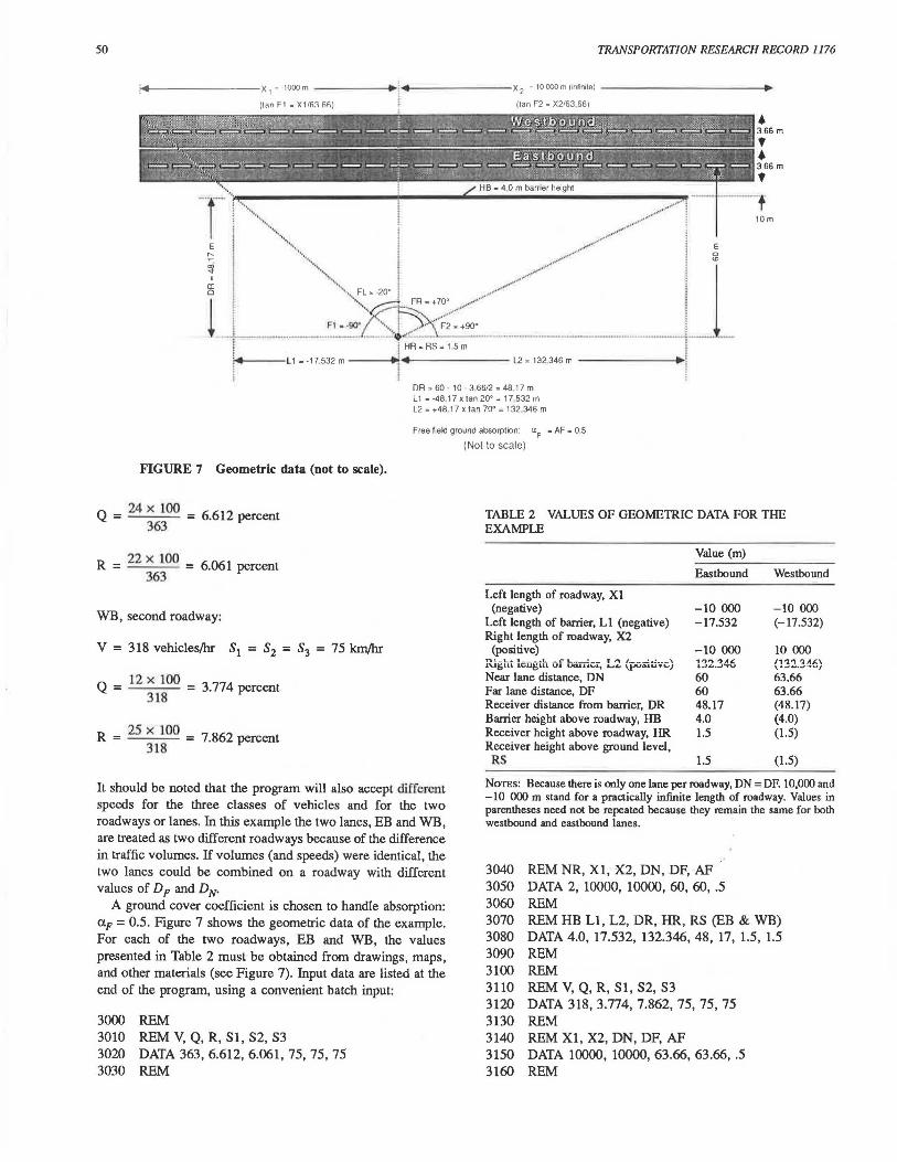
FIGURE 7 Geometric data (not to scale).

Q= 24 x 100 6.612 percent = 363

R 22 x 100 6.061 percent = = 363

WB, second roadway:

V = 318 vehicles/hr S1 = S2 = S3 75 km/hr

12 x 100 Q = = 3.774 percent 318

25 x 100 R = = 7.862 percent 318

It should be noted that the program will also accept different speeds for the three classes of vehicles and for the two roadways or lanes. In this example the two lanes, EB and WB, are treated as two different roadways because of the difference in traffic volumes. If volumes (and speeds) were identical, the two lanes could be combined on a roadway with different values of D F and DN.

A ground cover coefficient is chosen to handle absorption: aF = 0.5. Figure 7 shows the geometric data of the example. For each of the two roadways, EB and WB, the values presented in Table 2 must be obtained from drawings, maps, and other materials (see Figure 7). Input data are listed at the end of the program, using a convenient batch input:

3000 REM 3010 REM V, Q, R, Sl, S2, S3 3020 DATA 363, 6.612, 6.061, 75, 75, 75 3030 REM

TABLE 2 VALUES OF GEOMETRIC DATA FOR THE EXAMPLE

Value (m)

Eastbound Westbound

Left length of roadway, Xl (negative) -10 ()()() -10 000

Left length of barrier, L1 (negative) -17.532 (-17.532) Right length of roadway, X2

(positive) -10 ()()() 10 000 Ta! - L ... 1 _ __ .. L _r L - ---!-- T,, '---!..! •. -\ 132..346 11 "l.'1 'l AJ;\ n.i!;IU. .l'Vl.l~Lll U.l UCIJ..l.IV.L, .L.o• \JA'i3.lUV"'J , .......... ..,._,. .... , Near lane distance, DN 60 63.66 Far lane distance, DF 60 63.66 Receiver distance from barrier, DR 48.17 (48.17) Barrier height above roadway, HB 4.0 (4.0) Receiver height above roadway, HR 1.5 (1.5) Receiver height above ground level,

RS 1.5 (1.5)

NoTEs: Because there is only one lane per roadway, DN = DF. 10,000 and -10 000 m stand for a practically infinite length of roadway. Values in parentheses need not be repeated because they remain the same for both westbound and eastbound lanes.

3040 REM NR, Xl, X2, DN, DF, AF-3050 DATA 2, 10000, 10000, 60, 60, .5 3060 REM 3070 REM HB Ll, L2, DR, HR, RS (EB & WB) 3080 DATA 4.0, 17.532, 132.346, 48, 17, 1.5, 1.5 3090 REM 3100 REM 3110 REM V, Q, R, Sl, S2, S3 3120 DATA 318, 3.774, 7.862, 75, 75, 75 3130 REM 3140 REM Xl, X2, DN, DF, AF 3150 DATA 10000, 10000, 63.66, 63.66, .5 3160 REM

Jung and BlaMy

FREE FIELD NOISE LEVEL AND DELTA VALUES (EB)

CARS:

MEDIUM TRUCKS:

HEAVY TRUCKS:

51 822

51 .538

55.822

TOTAL, ALL VEHICLES: 58.304

15 . 157

13 ,878

9.649

NOISE AFTER BARRIER AND NET INSERTION LOSS, ALPHAB = 0

CARS: 48.360 3.46 I

MEDIUM TRUCKS: 48 204 3.331

HEAVY TRUCKS: 53.249 2.574

TOTAL, ALL VEHICLES: 55 391 2.913

FREE FIELD NOISE LEVEL AND DELTA VALUES (WB)

CARS:

MEDIUM TRUCKS:

HEAVY TRUCKS:

50.912

48. 142

55,991

TOTAL, ALL VEHJCLES: 57,678

14 ,210

12 .979

9.17 I

NOISE AFTER BARRIER AND NET INSERTION LOSS, ALPHAB = 0

CARS: 47,557 3.355

MEDIUM TRUCKS: 44,943 3 200

HEAVY TRUCKS: 53 582 2 409

TOTAL, ALL VEHICLES: 55.002 2 677

TOTAL NOISE BEFORE AND AFTER BARRIER, AND NET INSERTION LOSS

NUMBER BEFORE AFTER INSERTION LOSS

I CARS 54 401 50 988 3 413

2 MEDIUM TRUCKS 53. 174 49.885 3.290

3 HEAVY TRUCKS 58.918 56.429 2 489

4 TOTAL 61 OJ 3 58 2 I I 2 802

L.,q (BEFORE) L.,q (AFTER) I (FOR BOTH, EB & WO)

COMPARISON OF THE TOTAL WITH REFERENCE I, TABLE 4

BEFORE

61 1

AFTER

58.2

NET INSERTION LOSS

2. 9

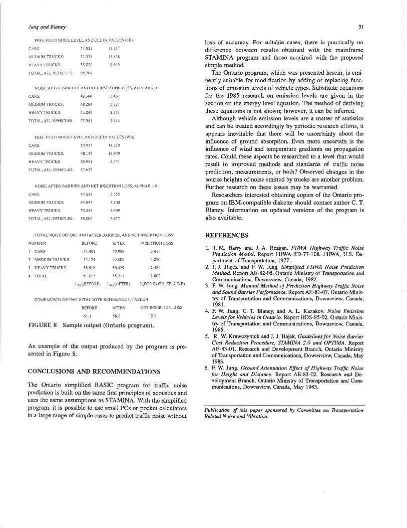
FIGURE 8 Sample output (Ontario program).

An example of the output produced by the program is pre­sented in Figure 8.

CONCLUSIONS AND RECOMMENDATIONS

The Ontario simplified BASIC program for traffic noise prediction is built on the same first principles of acoustics and uses the same assumptions as STAMINA. With the simplified program, it is possible to use small PCs or pocket calculators in a large range of simple cases to predict traffic noise without

51

loss of accuracy. For suitable cases, there is practically no difference between results obtained with the mainframe STAMINA program and those acquired with the proposed simple method

The Ontario program, which was presented herein, is emi­nently suitable for modification by adding or replacing func­tions of emission levels of vehicle types. Substitute equations for the 1985 research on emission levels are given in the section on the energy level equation. The method of deriving these equations is not shown; however, it can be inferred.

Although vehicle emission levels are a matter of statistics and can be treated accordingly by periodic research efforts, it appears inevitable that there will be uncertainty about the influence of ground absorption. Even more uncertain is the influence of wind and temperature gradients on propagation rates. Could these aspects be researched to a level that would result in improved methods and standards of traffic noise prediction, measurements, or both? Observed changes in the source heights of noise emitted by trucks are another problem. Further research on these issues may be warranted.

Researchers interested obtaining copies of the Ontario pro­gram on IBM-compatible diskette should contact author C. T. Blaney. Information on updated versions of the program is also available.

REFERENCES

1. T. M. Barry and J. A. Reagan. FHWA Highway Traffic Noise Prediction Model. Report FHWA-RD-77-108. FHWA, U.S. De­partment of Transportation, 1977.

2. J. J. Hajek and F. W. Jung. Simplified FHWA Noise Prediction Method. Report AE-82-05. Ontario Ministry of Transportation and Communications, Downsview, Canada, 1982.

3. F. W. Jung. Manual Method of Prediction Highway Traffic Noise and Sound Barrier Performance. Report AE-81-07. Ontario Minis­try of Transportation and Communications, Downsview, Canada, 1981.

4. F. W. Jung, C. T. Blaney, and A. L. Kazakov. Noise Emission Levels for Vehicles in Ontario. Report HOS-85-02. Ontario Minis­try of Transportation and Communications, Downsview, Canada, 1985.

5. R. W. Krawczyniuk and J. J. Hajek. Guidelines for Noise Barrier Cost Reduction Procedure, STAMINA 2.0 and OPTIMA. Report AE-83-01. Research and Development Branch, Ontario Ministry of Transportation and Communications, Downsview, Canada, May 1983.

6. F. W. Jung. Ground AttenuaJion Effect of Highway Traffic Noise for Height and Distance. Report AE-83-02. Research and De­velopment Branch, Ontario Ministry of Transportation and Com­munications, Downsview, Canada, May 1983.

Publication of this paper sponsored by Committee on Transporlalion­Related Noise and Vibration .