Hierarchical Component Using Reflective-Formative ......construct is namely Average Variance Extracted (AVE) proposed by Fornell & Larcker (1981). The formula of AVE is total factor

International Journal of Mathematics and Statistics Invention (IJMSI)

E-ISSN: 2321 – 4767 || P-ISSN: 2321 - 4759

www.ijmsi.org || Volume 2 || Issue 2 || February - 2014 || PP-55-71

www.ijmsi.org 55 | P a g e

Hierarchical Component Using Reflective-Formative

Measurement Model In Partial Least Square Structural

Equation Modeling (Pls-Sem)

Wan Mohamad Asyraf Bin Wan Afthanorhan

Department of Mathematics,

Faculty of Science and Technology,

Universiti Malaysia Terengganu, 21030 Kuala Terengganu, Malaysia

ABSTRACT: In recent years, partial least square structural equation modeling has been enjoyed popularly

since the various package for partial least square established. Besides, this method can be known as the the next

second generation modeling or soft modeling that can be a great helpful among the researchers and

practitioners to accomplish their objective research. In this paper also intend to modeling the second higher

order construct (Hierachical Component) as the advance in partial least structural equation modeling (PLS-

SEM) using smartpls which is the newest package. In this application of this method, we can create a higher

order construct, in particular, the reseracher should empahsize for many aspect in order to ensure this model is

more relevance and significant. Thus, the application using reflective-formative should be carry out in order to

obtain the best model. In some instance, the author present the guideline to conduct this analysis with a real

example so that the researchers outside will be more understanding and enjoyed for this new application.

KEYWORDS: Partial Least Square Structural Equation Modeling, Hierarchical Component Model, Second

Order Construct, Reflective-Formative Model, SmartPls

I. INTRODUCTION PLS-SEM has been established for a long time ago by Wold (1982), however, this method is not

popular as covariance based structural equation modeling (CB-SEM) in which focuses on goodness of fitness to

minimize the covariance matrix and estimation matrix (Hair, 2010) earlier 1980. However, CB-SEM has a lot

weakness since the reserchers should be ensure the model has achieved requirement before subsequent analysis

in the structural model. In this case, the researcher has been spent time to focus on goodness of fit rather than

estimation or prediction.

Therefore, the introduction to PLS-SEM is returned now with a great helpful and more user friendly to

curb the problem of researchers nowadays. In the accordance with Hair (2010) discover the PLS-SEM is aimed

to maximize the explained variance of the endogenous construct (square multiple correlation, R2) of the

endogenous latent construct (dependent).

This application is performed nonparametric analysis in which does not rely on distributional

assumption (Chin, 1998). Thus, this method is appropriate for those who have insufficient data, time and others.

However, PLS-SEM is does not assume data to be normal even it appropriate for nonparametric. Thus, the

bootstrap in smartpls is used to resampling the data until the data meet the result. According to Byrne (2010),

bootstrap is an aid for nonparametric data in structural equation modeling.

Hair (2010) listed several advantages for those who apply PLS-SEM:

Normality of data distribution not assumend normality

Can be used with fewer indicator (manifest variable)

Models can be include a larger number of indcator variable

Preffered alternative with formative construct Assumes all measured variance (including error) is useful for explanation/prediction of causal relationship

The result obtained in t-distribution against CB-SEM since this method is performed nonparametric

analysis. In addition, the researcher does not have difficult to apply the formative construct in PLS-SEM.

Formative construct in CB-SEM is much complicated than PLS-SEM and, of course, PLS-SEM ease the

researchers to perform their analysis regarding on their objective research.

Hierarchical Component Using Reflective-Formative…


II. FORMATIVE AND REFLECTIVE MEASUREMENT MODEL In the accordance with Hair (2010) explain measurement model is the process of assigning numbers to a

variable/construct based on a set of rules that are used to assign the numbers to the variable in a way that accurately

represents the variable. Measurement model have two type which is reflective and formative construct.Usually, researchers

endorsed to apply reflective costruct since it much better to conduct the analysis rather than formative. But PLS-SEM defy

this thereotically and they have a chance to perform second higher order construct in structural equation modeling. These

two measurement model have various purpose but some researchers still confuse to apply its application. Some of them just

assume all the measurement model is reflective construct. Therefore, Ringle (2008) has established one article about the

Confirmatory Tetrad Analysis in PLS-SEM (CTA-PLS) to differentiate between reflective and formative construct. In this

instance, the reserachers should meet the requirement of the bootsrapping confidence interval, composite reliablity and VIF.

In this paper intend to address the herarchical component analysis using PLS-SEM type II (Reflective-Formative) model.

Reflective measurement model is a type of measurement model setup in which the direction of the arrow is from

the construct to the indicator (manifest variable), indicating the assumption that the construct causes the measurement model

(more precisely, the covariation) of the indicator variables (Hair et.al, 2013). Reflective model is performed when the

statement is related on the effect of variable. Therefore, the arrow is pointing outward from latent construct imposed on

manifest variable.

Formative measurement model is a type of measurement model setup in which the direction of the arrow is from

indicator variables to construct, inidcating the assumption that the indicator variable cause the measurement of the construct

(Hair, 2013). Formative model is performed when the satement is related on the cause of variable. Therefore, the arrow

pointing inward from manifest variable imposed on construct.

In this case, the author intended to apply both measurement models in structural model in order to create a second

higher model. A higher model should be taken into account for each relevace and significant, in particular, researcher should

be considered to achieve the requirement for reflective and formative construct.

Generally, reflective measurement model are widespread and only a small proportion of SEM-based studies have applied for

formative measurement model. On the use of reflective measurement model become a normal practice among researchers to

examine their relationship between exogenous and endogenous constructs. In particular, reflective measurement model is

much ease to handle rather than formative measurement due to the reflective construct is focus on relevance of indictor

while formative construct focus on significant of indicators.

III. ASSESSING OF REFLECTIVE MEASUREMENT MODEL Following the validation guidelines of Straub et al. (2004) and Lewis et. Al (2005), the reflective measurement

model should be tested at least unidimensionality procedure, internal consistency reliability, indicator reliability, convergent

validity and discriminant validity in order to achieve the fitness of measurement model. Unidimensionality procedure cannot

be conducted directly from PLS-PM, but can be assessed by exploratory factor analysis (EFA) that can be installed in

various packages such as SPSS, SAS, MINITAB, EVIEWS and others. Unidimensionality is aimed to drop the item that

consists less contribution on these factors. Accurately, the procedure for removal items had two types which is

multidimensionality and unidimensionality procedure. Both these procedure plays a same vital role to retain the item which

are related on the factor though these procedure looks so different to carry out the research. Usually, researchers prefer value

below than 0.50 should be drop from the measurement model (Afthanorhan. 2013). However, it depends on researchers to

choose which one of the substantive meaningful regarding on their literature review. In this case, the author addressed 0.60

or above of factor laodings to retain in the measurement model.

Once the unidimensionality procedure has achieved, the traditional method which is internal consistency

reliability, Cronbach alpha proposed by Nunnally (1978) has been used. As usual, value higher than 0.70 considered as the

meausrement model is reliable. But there is an alternative method tu replace the wekaness of cronbach alpha namely

composite reliability. Composite reliability is proposed by Nunally and Bernstein (1994) and most of the researchers concurs

to indicate this method is much relible rather than cronbach alpha, since this measure managed to overcome some of

cronbach alpaha deficiency.

According to Urbach et. al (2010), indicator reliability describe the extnet to which a variable or set of variables is

consistent regarding what it extends to measure. However, in PLS-SEM does not emphasize the purpose of indicator

reliability, instead, the significant of indicator can be tested using resampling tecnique such as bootstrapping (Efron 1979) or

jacknifing (Miller 1974). There may be various reasons for these requirement not beong fulfilled since the item may ghave

influenced by additional factors that can give the untrue estimation. Thus, PLS algorith initiated once more in order to obtain

new results.

Convergent validity involves the degree to which individual items reflecting a construct converge in comparison to

items measuring different constructs (Urbach et. al, 2010). A common criterion applied to test the convergent validity

construct is namely Average Variance Extracted (AVE) proposed by Fornell & Larcker (1981). The formula of AVE is total

factor loading power of two divide by number of items consisted. Fornell & Larker suggest the result higher than 0.50

indicate the construct is captured to be explained more than half of the variance of its indicators and thus, demonstrates

sufficient convergent validity. In particular, any value in construct below than 0.50 is consists of measurement residual.



Finally,discriminant validity concerns the degree to which the measures of different constructs differs from one

another. According to Zainudin (2013), the correlation between exogenous variabes (independent) should be below 0.85 to

prove the constructs differs contributions. For the first measures, cross laodings are obtained by correlating each latant

variable component scores with all the other items (Chin, 1998). Accordingly, the AVE of each latent variable should be

greater than the constructs highest square correlation with any other latent variable.

Validity Type Criterion Description Literature

Unidimensionality Exploratory

Factor Analysis

(EFA)

The number of selected factors is determined by the

numbers of factors with an eigentvalue greater than 1.0.

Gerbing and

Anderson (1988)

Internal

Consistency

Reliability

Cronbach Alpha Should be greater than 0.70 to achieve the reliable of

measurement model

Nunally (1978)

Internal

Consistency

Reliability

Composite

Reliability

Alternative to Cronbach Alpha that attempt to measure

the sum of an LV‟s factor loadings relative to the sum of

the factor loadings plus error variances

Nunally and

Bernstein (1994)

Indicator Reliability Indicator

Loadings

Measures how much of the indicators variance is

explained by the coresponding latent variables.

Chin (1998)

Convergent Validity Average Variance

Extracted (AVE)

Proposed threshold value for AVE should be higher tahn

0.50

Fornell and

Larcker (1981)

Discriminant

Validity

Fornell-Larcker

criterion

The AVE of each latent variable should be greater than

the latent variable highest squared correlation with any

other latent variable

Fornell and

Larcker (1981)

Exhibit 1

IV. ASSESSING OF FORMATIVE MEASUREMENT MODEL The validation of formative measurement model requires a different approach than the reflective

measurement model. Conversely, conventional validity assessments do not apply to formative measurement

models, and the concepts of reliability and construct validity are not meaningful when employing such models

(Bollen 1984; 1989). According to Ringle et. al (2013), the assessment of the formative constructs convergent

validity by examining its correlation with an alternative measures of the constructs, using reflective measures or

a global single item. The correlation between the construct should be higher than 0.80.

The collinearity should be considered in formative measurement model in the subsequent analysis.

Thus, tolerance represents the amount of variance of one formative indicator not explained by the other

indicators in the same block. Each indicator tolerance VIF should be in range between 0.20 and 5.0. Otherwise,

obliterate indicators, merging indicators in a single measure, or creating higher order construct to treat

collinearity problem. The higher order construct consists of four type that has been suggested by Ringle (2011)

as well as Hanseler (2009). In this instance, the author intend to apply second order construct type II or higher

component model (HCM) type reflective-formative measurement model.

The prior assessment in higher order construct should be test each indicator‟s outer weight and outer loadings as

well. The resampling technique is used here to assess their significance for each indicator. When indicator weight (factor

loading for formative construct) is significant, there is empirical support to retain the indicator. Nevertheless, when an

indicators weight is not significant but the corresponding outer loading is significant (factor loading for reflective

measurement model > 0.60), the indicator should be retained.In short, if both outer loading and outer weight is non-

significant, there is no empirical support to retain the indicators it should be dropped from the model. Apparently, the

researchers should illuminate the reasons to retain or delete the indicators by examining its pedagogical theoretical relevance

(reflective) and importance (formative) of the same constructs.

If the theory driven conceptualization of the construct strongly supported retaining the indicators, it should be kept

in the formative constructs. But, if the conceptualization does not strongly support an indicator inclusion, the insignificant

indicator should most likely to be removed (Ringle et. al, 2013). In contrast, if the outer loading is low and non-significant,

there is no empirical support to retain the indicator in a model (Cenfetelli & Bassellier, 2009). Therefore, such an indicator

should be removed from the formative measurement model to equip their fitness with significant of relevance and

importance.

Accordingly, both significant and insignificant formative indicators should be kept in the measurement model as

long as this is conceptually justified (Henseler et al. 2009). Unlike the reflective measurement model that should be achieve

their conventional validity. The different criterion for assessing formative construct is summarized in exhibit table below:



Validity Type Criterion Description Literature

Indicator

Validity

Indicator weight The reflective measurement model should be

achieve their relevance in which higher than

0.60. Some of the authors also recommend

path coefficient (estimation) should be

greater than 0.10 or 0.20

Chin (1998b),

Lohmöller (1989)

Indicator

Validity

Variance Inflaction

Factor (VIF)

Indicates how much of an indicators variance

explained by other influences in a model.

Should be higher than 0.20 but lower than

5.0. Otherwise, remove indicator, emerging

in single index, or create higher order

construct.

Cassel and Hackl

(2000), Diamantopoulos

and Siguaw

(2006), Fornell and

Bookstein (1982),

Gujarati (2003), Ringle et.al

(2013)

Construct

Validity

Interconstruct

Correlations

If the correlation between construct is below

than 0.85 indicates that the constructs is

differ sufficient from one another. The differ

sufficient provide an importance construct.

Mackenzie et al.

(2005), Bruhn et al.

(2008)

Exhibit2

V. SINGLE ITEM AND MULTIPLE ITEM MEASURES Single item is very rarely to be used among researcher when comes to determine the interrelationship between

exgenous and endogenous construct. However, single items have practical advantages such as ease of application, brevity,

and lower costs associated with their use (Hair et. al, 2013). In CB-SEM application, single item cannot be handling when

the reserachers intend to use unidimensionality procedure due the identification problem. Identification issues usually exist

when the latent construct consists below four indicators. This is because the data cannot be computed since the lower degree

of freedom. Thus, the reserachers figure out another ways to solve this problem. They established pooled confirmatory factor

analysis CFA since this application can be handle the construct below than four. But PLS-SEM is much easy to handle since

this method can use a single item for estimation. Note that, contrary to commonly held beliefs, single item reliability can be

estimated (Loo, 2002; Wanous, Reichers, & Hudy, 1997). Most importantly, from a perspective, opting a single item

measures in most empirical settings is a risky decision when it comes to predict vaidity considerations.

Multiple items measures have been interested among the researchers to analyze their data. They developed the item

based on their literature and of course the result obtained would be less decison risk since multiple measure encomprises for

whole aspect relevance. Once again CB-SEM present their weakness when this application cannot be handled when items is

too many and as usual PLS-SEM is the alternative method to overcome these issues. Therefore, PLS-SEM has been popular

lately since this application is user friendly and more understanding.

VI. HIERARCHICAL COMPONENT MODEL USING PLS-SEM IN SMARTPLS 2.0 Hierarchical latent variable models, hierarchical component models, or higher-order constructs, are explicit

representations of multidimensional constructs that exist at a higher level of abstraction and are related to other constructs at

a similar level of abstraction completely mediating the influence from or to their underlying dimensions (Chin, 1998b). Law

et al. (1998, p. 741). Establishing such a higher model component usually called in the context of PLS-SEM

(Lohmoller,1989) most often involve testing second oder constructs that contain two layers of constructs.

In generals, hierarchical component model (HCM) is rarely been used since this modeling implement for two stage

approach. Two stage approaches is initiated once the researchers apply for formative measurement model. Unfortunately,

some of researchers grouse to determine whether their model is appropriate for reflective or formative measurement model.

Therefore, Hair (2009) introduce to Confirmatory Tetrad Analysis (CTA-PLS) to guide the researchers differentiate these

measurement model. Additionally, there are threefolds for the inclusion of an HCM in PLS-SEM. First, by establishing

HCMs, researchers can reduce the number of indicators in a structural model besides making the model more parsiminous

and ease to to grasp. Secondly, HCMs prove valuable if the construct are highly correlated. In statistics regression, a highly

correlated tends to exist the multicollinearity problem. Thus, the estimation of the structural model may be biased due to the

collinearity issue and the conventianal validity cannot be feasible. In situations characterized by collinearity among

constructs, a second order can remedy such collinearity issues and may solved discriminant validity. Thirdly, establishing of

HCMs can also prove valuable if formative indicators exhibit high levels of collinearity. Provided that theory supports this

step, researchers can split up the set of indicators and establish separate constructs in a higher order structure (Ringle et. al,

2013). Forth, formative measurement model in PLS-SEM is much ease to handle rather than CB-SEM that can ascertain the

researcher to consider for both measurements at one time. Fifth, the result provided also include for formative and reflective

mesurement model, thus, the researchers can make a comparison for both measurement. Sixth, modeling hierarchical

component model is useful for researchers to reframe the structure model to be more meaningfull besides to address the

predicton rather than the process of evaluation in structural model. Sevently, introduction to hierarchical component model

proposed by Ringle (2012) in PLS-SEM causes some of the researchers in curious to determine the comparison of these

component model, therefore, modeling of HCMs widespread and enjoyed to popularly applied.



HCMs prove as the higher order model since the researchers should ensure all the requirements and evaluation

coincide the concept of advance in PLS-SEM. Instead of CB-SEM in which rely on distributional assumption before further

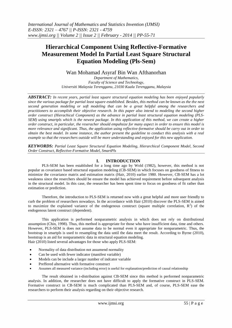
the analysis, PLS-SEM is managed to increase the explained total variance in each constructs. Exhibit 3 illustrates the four

main types of HCMs discussed in the extant literature (Jarvis et.al, 2003; Wetzels et al.,2009) and used in applications

(Ringle, 2012). These types of model have two elements: the Higher Order Component (HOC), which captures the more

abstract entity, and the lower order component (LOC) which captures sub-dimensions of the abstract entity. Each of the

HCMs types is characterized by different relationship betwen the HOC and LOCs and construct and their indicators.

Reflective-Reflective Type I Reflective-Formative Type II

Formative-Reflective Type III Formative-Formative Type IV

Types of Hierarchical Component Model (Ringle et al.,2012)

Note: LOC = Lower- Order Component; HOC = Higher-Order Component



One of the most applied in structural equation modeling among researchers nowadays is Reflective-Reflective

Measurement Model known as Second Order Construct Type I. In particular, the causal path of lower-order constructs are

imposed on associated of observed variable (item) enclosed in rectangular shapes and at the same time the causal path of

higher order constructs is exert on lower order constructs. Lohmoller (1989) calls this type of model „hierarchical common

factor model‟, where the higher order construct represents the common factor of several specific factors. Unfortunately, Lee

& Cadogan (2005) state to deny this theoretical structure model and classify that there is “no such thing” as reflective-

reflective heirarchical latent variable model and such a model is “at worst. Misleading, and at a best meaningless”.

Second, on the Reflective-Formative Type II model as presented in this paper later on with the

guidelines given to ascertain researchers outside to practice HCMs in PLS-SEM. In contrast, modeling

reflective-formative type II is slightly difference compare to previous HCM, in which the causal path of lower

order constructs is exert on higher order construct. In other words, higher order construct is automatically to be

formative construct to play a double explanation comprises of reflective and formative measurement model is

structural model.According to Chin (1998) clarify the lower-order constructs are selectively measured constructs

that do not share a common cause but rather form a general concept that fully mediates the impact on

subsequent endogenous variables. Sometimes, these types of hierarchical latent variables are also used to

account for the measurement error of the indicators of a “normal” formative construct: the indicators are

operationalized as reflective constructs to explicitly model their measurement error (Cadogan and Lee, in press;

Edwards, 2001).

Third, in the Formative-Reflective Type III model is slightly difference compare to reflective-

formative type II as the explanation above. In this instance, a higher construct model will be imposed by each

manifest variable (indicators) and at the same time the causal effect from higher order construct exert on lower

order construct that comprises of indicator. Of dealing this application should be initiated on VIF to achieve the

requirement of formative measurement model. Once finish the initial step, convergent and discriminant validity

should be measured as usual upon to modeling the structural model. In addition, Ringle (2011) also proposed of

this application so that researcher could examine the difference between reflective-formative and formative-

reflective. Different types of model explain the difference purpose of the study.

Lastly, in the Formative-Formative Type IV model is the most rare to be implement in the structural

model. Of this application is appropriate when both of HCMs and LCM is in the form of formative constructs.

Yet, this application renowned as the higher model or two stage approach. If researchers interest to apply of this

application, should be illuminate reasons and example of the questionnaire. Thus, the readers will be more

understood the purpose of this application.

VII. MEASUREMENT INSTRUMENTS

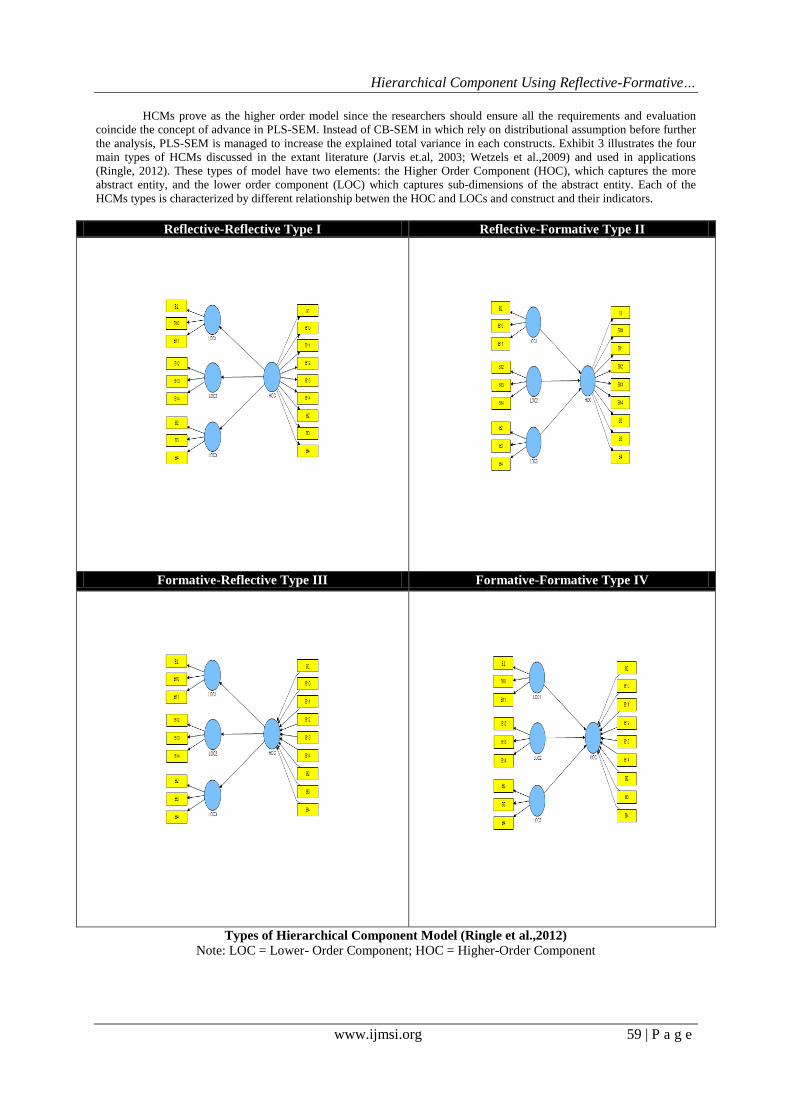
In this paper provided for five constructs namely motivation, goverment support, challenge, barrier and

benefits that has been validated using the past previous literature. These variables once to outline the level of

involvement in voluterism program among youth but now the author intend to address the HCMs in PLS-SEM

using these variables as a research subject. The questionnaire has been distributed to five higher education

chosen using stratified sampling technique and involving 453 respondents. Generally, questionnaire designed a

total of 53 items in each difference variables so that the respondent know the aimed of question given. The likert

scale used is from 1 through 5 (1- strongly disagree. 2- disagree, 3- undecided, 4- agree, 5- strongly agree). As

usual, the researchers should ensure all the items loading in data set has been standardized (mean = 0, standard

deviation =1). If not, the result obtained in confirmatory factor analysis consists of negative value. Means that,

the item consists of factor loading do not have the same direction on endogenous variables.

VIII. FIVE VARIABLES On the use of five variables represent for five measurement models will be apply using PLS-SEM. All

of these factors are chosen by the previous literature to examine the level of participation in volunteerism

program. Yet, in order to accomplish the objective research to create a higher model, of course, the author

deserve to highlight the method of statistical modeling rather than to imply on the prediction of these variables.

These five variables included in a structural model will be test to undergone the process of hierarchical

component analysis. Theoretical framework is presented as below:



Figure 1

IX. RESULT AND FINDINGS Previously, the reflective measurement model should be determined to drop the indicator which has

less contribution in a model. In particular, this procedure namely unidimensionality or multidimensionality

procedure is aimed to drop the indicator (items) below 0.60. Otherwise, indicators should be retained in a model

and subsequent analysis will be feasible to create a higher model. Again, a higher order model could be

performed when the second order construct employ in a structural model. In this instances, the researchers

should ensure all of the factor loadings obtained triumph the same direction and highly significant. Once the

multidimensionality procedure has been conducted, the composite reliability, convergent and discriminant

validity should be performed. Repeatedly, structural model is inadmissible once reliability and validity fail to

meet the requirement since this approach has been acknowledge for all infamous researchers.

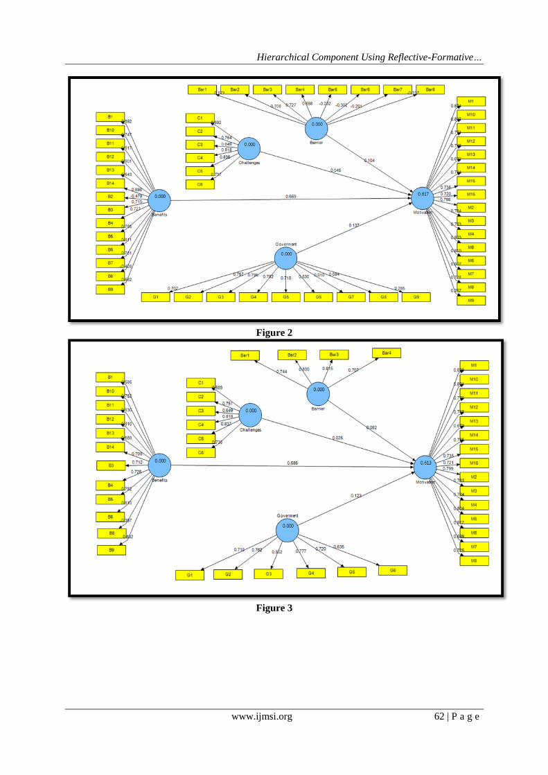
The figure 2 presented measurement model for whole construct after having PLS algorithm. PLS

algorithm is supportive to provide the factor loading for each manifest variable (indicators) encomprises in each

constructs. The value obtained can be seen between manifest variable and latent construct in which upper causal

path. By inspecting through the value obtained in structural model, researchers could recognize which value has

less factor loading. The lower factor loadings indicate the lower contribution on these factors. Once researchers

identify the lowest factor loading (< 0.60), an item should be deleted at once in a time to meet the minimum

criterion. Most of the researchers knew the process to conduct multidimensionality procedure but the way they

used is still incorrect. To make the better approach in multidimensionality procedure, researchers should drop

the lowest factor loading once in a time, and repeat this process untill meet the requirement to achieve upper

than 0.60.

In order to avoid from an ambiguity explanation, let see the Figure 2 presented, the first thing is certify

all the factor loading having the same direction (all positive value) in each constructs. In this case, the latent

(unobserved) construct have four manifest variable (indicators) namely Bar5, Bar6, Bar7, and Bar8 consist in

negative value. Means that, these manifest variable should be recoding since having the vice versa direction

(e.g: 5 = strongly disagree, 4 = disagree, 3 = undecided, 2 = agree, and 1 = strongly agree) using other

application such as SPSS or ther appropriate package. Usually, perceived negative value obtained caused by

negative statement in questionnaire provided. Therefore, the author re-do the latent construct for Barrier only

and re-run the analysis using PLS algorithm. Finally, the result in confirmatory factor analysis is achieved the

same direction (all positive value) and the subsequent analysis to identify the lowest factor loading as the

explanation has been given.

The multidimensionality procedure is conducted untill meet the requirement as presented in Figure 3. To be more

undoubtedly, researchers outside should be show their step by step before show the final modeling in multidimensionality. In

this case, the author skip several step since the current paper is to outline the hierarchical component model (HCM). Thus,

the result for confirmatory factor analysis can bee see in “A Comparison of Partial Least Square Structural Equation

Modeling and Covariance Based Structural Equation Modeling for Confirmatory Factor Analysis” written by Afthanorhan

(2013). This article will guide researchers to apply the confirmatory factor analysis using PLS-SEM and an advantages PLS-

SEM in multivariate analysis. Once the reflective measurement achieve the requirement, now author proceeds the formative

construct (Figure 4) to equip a second higher order construct (reflective-formative construct).



Figure 2

Figure 3



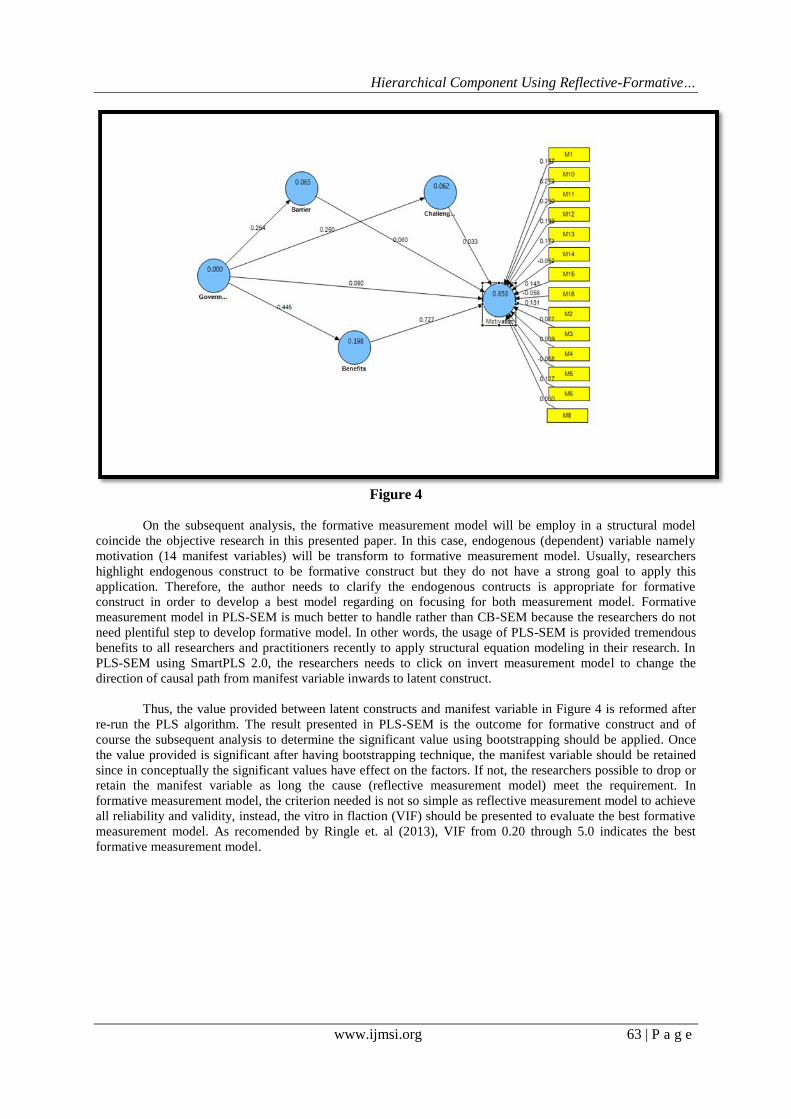
Figure 4

On the subsequent analysis, the formative measurement model will be employ in a structural model

coincide the objective research in this presented paper. In this case, endogenous (dependent) variable namely

motivation (14 manifest variables) will be transform to formative measurement model. Usually, researchers

highlight endogenous construct to be formative construct but they do not have a strong goal to apply this

application. Therefore, the author needs to clarify the endogenous contructs is appropriate for formative

construct in order to develop a best model regarding on focusing for both measurement model. Formative

measurement model in PLS-SEM is much better to handle rather than CB-SEM because the researchers do not

need plentiful step to develop formative model. In other words, the usage of PLS-SEM is provided tremendous

benefits to all researchers and practitioners recently to apply structural equation modeling in their research. In

PLS-SEM using SmartPLS 2.0, the researchers needs to click on invert measurement model to change the

direction of causal path from manifest variable inwards to latent construct.

Thus, the value provided between latent constructs and manifest variable in Figure 4 is reformed after

re-run the PLS algorithm. The result presented in PLS-SEM is the outcome for formative construct and of

course the subsequent analysis to determine the significant value using bootstrapping should be applied. Once

the value provided is significant after having bootstrapping technique, the manifest variable should be retained

since in conceptually the significant values have effect on the factors. If not, the researchers possible to drop or

retain the manifest variable as long the cause (reflective measurement model) meet the requirement. In

formative measurement model, the criterion needed is not so simple as reflective measurement model to achieve

all reliability and validity, instead, the vitro in flaction (VIF) should be presented to evaluate the best formative

measurement model. As recomended by Ringle et. al (2013), VIF from 0.20 through 5.0 indicates the best

formative measurement model.



Statement VIF

I want to learn something new. 1.707

I want to work with people 2.839

I feel it is my duty as a citizen. 2.787

It fulfills my moral principles. 2.969

I see it as the opportunity to make a difference. 3.069

I want to help community. 2.976

I want to improve my resume. 1.781

I want to occupy my free time. 2.158

It is a requirement/expectation by university, faculty, school, religious center or

another agency.

1.285

Volunteering is good for my professional development. 2.618

Volunteering gives me the opportunity to make new friends. 2.472

I believe my skills can be useful to the community 2.259

Volunteering is a social stimulation 1.804

I enjoy the volunteer activities 2.612

I want to help my society or close friends 2.119

Volunteerism helps me feel better about myself 2.236

Exhibit 3

As we can see in Exhibit 3, all VIF provided in each manifest variable is achieve the requirement for

formative measurement model. Previously, the author outlined the endogenous variables only, thus the result for

motivation construct should be adequate to subsequent analysis on herarchical component analysis. VIF can be

analyzed using various packages such as SPSS, Eviews, Minitab and others. In this case, the author using SPSS

to obtain the collinearity statistics for motivation constructs in order to achieve the criterion for formative

construct. On focusing of hierarchical component analysis, all manifest variable enclosed in rectagular

associated in motivation construct will be condensed to 7 newly latent constructs. In other words, the manifest

variable provided initial of 14 items will be divided into each established latent constructs (e.g: M1 and M10 =

MA, M11 and M12 = MB, M13 and M14 = MC and so forth). The establishing new latent construct can help the

researcher grasp a result and elude confused in a structural model. Additionally, all the established new latent

construct should be pointing on motivation construct (endogenous) while other all manifest variable enclosed in

rectangular pattern should be hide in measurement model (motivation) so that the modeling of second order

higher construct will be more clearly and orderly. Once again PLS-SEM show the powerful analysis when this

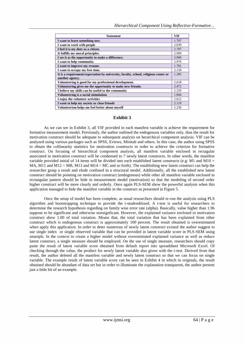
application managed to hide the manifest variable in the construct as presented in Figure 5.

Once the setup of model has been complete, as usual researchers should re-run the analysis using PLS

algorithm and bootstrapping technique to provide the t-studenditized. A t-test is useful for researchers to

determine the research hypothesis regarding on family wise error rate (alpha). Basically, value higher than 1.96

suppose to be significant and otherwise nonsignficant. However, the explained variance enclosed in motivation

construct show 1.00 of total variation. Means that, the total variation that has been explained from other

construct which is endogenous construct is approximately 100 percent. The result obtained is overestimated

when apply this application. In order to deter numerous of newly latent construct existed the author suggest to

use single index or single observed variable that can be provided in latent variable score in PLS-SEM using

smartpls. In the context to create a higher model without overestimated explained variance as well as reduce

latent construct, a single measure should be employed. On the use of single measure, researchers should copy

paste the result of latent variable score obtained from default report into spreadsheet Microsoft Excel. Of

checking through the value, the product for newly latent variable also given with the t-test. Derived from that

result, the author deleted all the manifest variable and newly latent construct so that we can focus on single

variable. The example result of latent variable score can be seen in Exhibit 4 in which in originals, the result

obtained should be abundant of data set but in order to illuminate the explanation transparent, the author present

just a little bit of an example.



Figure 5

Barrier Benefits Challenge Goverment Motivation

0.3002 -0.2203 1.8848 0.1549 -0.3678 -0.1003

0.6967 -0.2219 0.6658 0.7362 -0.3678 -0.5203

0.3002 0.9345 0.6658 0.1549 0.312 0.4847

-0.0436 0.7945 -0.1982 1.3689 1.0028 1.2464

-0.6848 0.9121 -0.9482 -1.9017 0.323 0.0348

-0.3244 0.5105 0.6019 0.8031 -1.0586 0.2743

1.7075 0.8044 1.5547 -0.4353 1.0028 1.1444

-1.1071 0.2507 0.2553 -1.615 0.312 0.9087

0.3002 1.0514 -0.1591 1.3689 0.323 0.4709

Exhibit 4

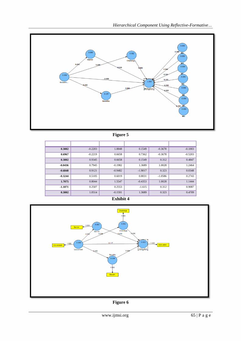
Figure 6



Using on the same structural model, the researchers should create a new project in Smartpls to use a

new data set that will be implement in the structural model. As mention earlier, the author intend to use the

single measurement index in a structural model, of course, the researchers should re-do the analysis using new

indicator provided from new data set. In shortly, latent variable score mainly from Exhibit 6 will be

implementing in Figure 6. Now, lets examine the explained variance in endogenous constructs namely

motivation, variance is totally difference rather than previous one in particular (Figure 5 = 1.000 to Figure 6 =

0.603) plus can be proved that the single measurement indicator also can be helpful in data analysis. Yet,

analysis on hierarchical component analysis should not be stopped here since the author intend to address the

most significant impact using five variables in partial least square. In social science, significant impact between

construct is prior to determine positive relationship, negative relationship as well as the impact of research

applied using statistical methods.

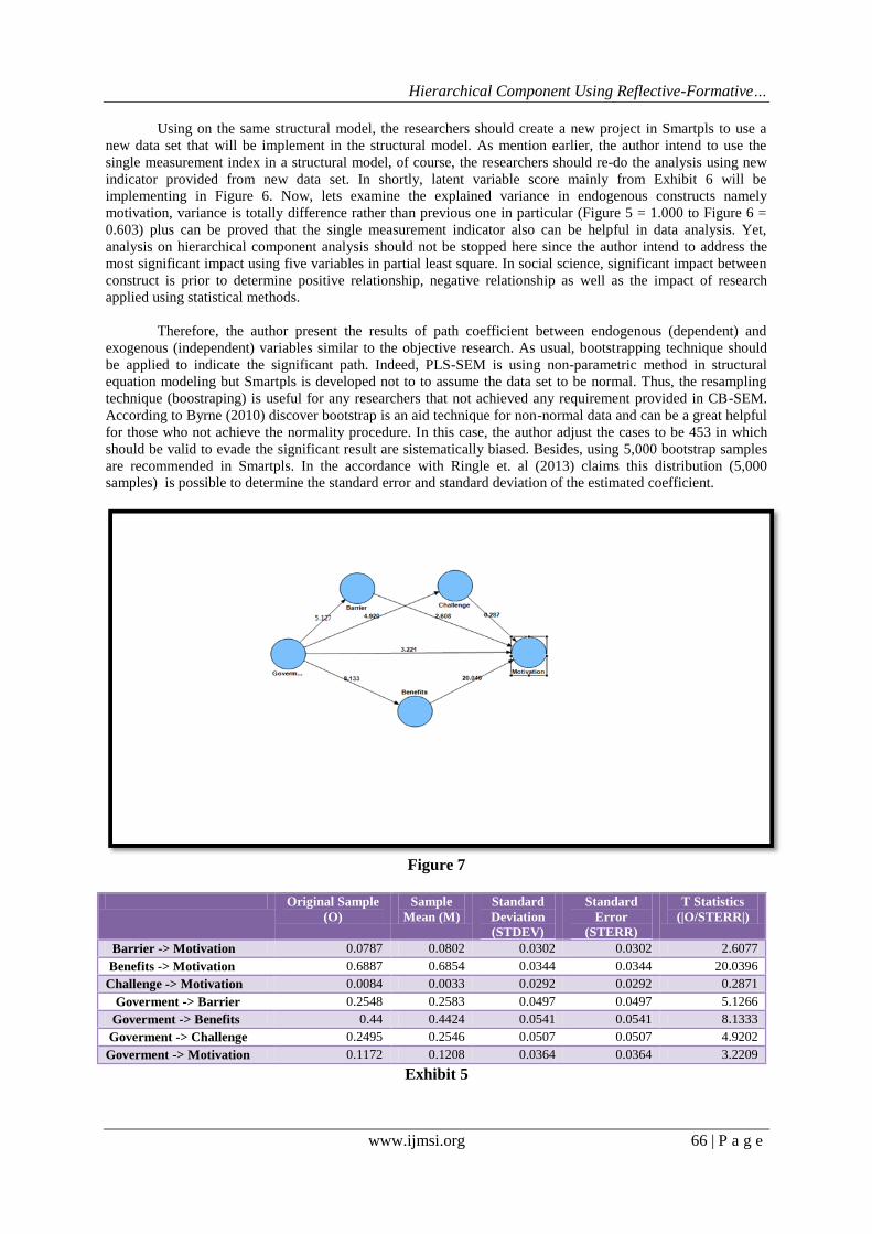
Therefore, the author present the results of path coefficient between endogenous (dependent) and

exogenous (independent) variables similar to the objective research. As usual, bootstrapping technique should

be applied to indicate the significant path. Indeed, PLS-SEM is using non-parametric method in structural

equation modeling but Smartpls is developed not to to assume the data set to be normal. Thus, the resampling

technique (boostraping) is useful for any researchers that not achieved any requirement provided in CB-SEM.

According to Byrne (2010) discover bootstrap is an aid technique for non-normal data and can be a great helpful

for those who not achieve the normality procedure. In this case, the author adjust the cases to be 453 in which

should be valid to evade the significant result are sistematically biased. Besides, using 5,000 bootstrap samples

are recommended in Smartpls. In the accordance with Ringle et. al (2013) claims this distribution (5,000

samples) is possible to determine the standard error and standard deviation of the estimated coefficient.

Figure 7

Original Sample

(O)

Sample

Mean (M)

Standard

Deviation

(STDEV)

Standard

Error

(STERR)

T Statistics

(|O/STERR|)

Barrier -> Motivation 0.0787 0.0802 0.0302 0.0302 2.6077

Benefits -> Motivation 0.6887 0.6854 0.0344 0.0344 20.0396

Challenge -> Motivation 0.0084 0.0033 0.0292 0.0292 0.2871

Goverment -> Barrier 0.2548 0.2583 0.0497 0.0497 5.1266

Goverment -> Benefits 0.44 0.4424 0.0541 0.0541 8.1333

Goverment -> Challenge 0.2495 0.2546 0.0507 0.0507 4.9202

Goverment -> Motivation 0.1172 0.1208 0.0364 0.0364 3.2209

Exhibit 5



Figure 7 and Exhibit 5 display the final model of hierarchical component analysis through PLS

algorithm and bootstrapping technique. By inspecting through t-statistics at the last column in Exhibit 7, almost

latent construct indicates have singnificant impact on each other unless one pair construct which is construct of

challenge and motivation. With the accordance of Hair et. al (2010) uncover any value in t-test should be higher

than 1.96 (a < 0.05) indicates achieved significant level (95% confidence interval). Otherwise should be classify

as insignificant or nonimpact occurs.

The first things is the researchers should identify whether the constructs is in positive or negative

relationships, afterwards uncover the most contribution factors triggered on this research. In this instances, all of

the variables include in a structural model are positive relationship, means that the direction of respondent

towards these factors are positive. Mean while, indirect factors involving benefits, barrier and challenges on

motivation revealed that benefits factor is the most crucial towards voluteerism program. In conceptually,

benefits construct is plausible to consider as the most contribute parallel to the past research. In perpendicular,

indirect effect of challenge on motivation (dependent) is perceived insignificant impact. For some instance,

challenge factor does not give significant impact on motivation, means that the existence of this factor is failed

to provide a significant impact towards this reserach subject. Of standard deviation and standard error is a

similar perspective because both parameter is drawn from sample in population. Likewise, standard errors that

are extremely large indicate parameters that cannot be determined (Joreskog & Sorbom, 1993). Because

standard error are influenced by the units of measurement in observed and/ or latent variables, as well as the

magnitude of the parameter estimate itself, no definitive criteria of small and large have been established

(Joreskog & Sorbom, 1989).

In this instance, model estimation provided on the basis of PLS algorithm and bootsrapping sampling

are helpful to minimize standard error and deviation in the model. Standard error reflects the precision with

which a parameter has been estimated, with a small values suggesting accurate estimation. Nevertheless, most

researchers do not emphasize this issue on their report because the aimed of the research is to evaluate and

provide a good precison using a particular step approach.

X. CONCLUSION AND RECOMMENDATION For some instances, as usual, one conclusion should be made regarding on our analysis so that the

readers will discern our contribution for this research. A second order construct can be known as two stage

approach once the implementation of formative measurement model in a structural model. In this instance, we

should ensure all the outer loadings and outer weights meet the requirement based on our literature previous.

Afterwards, establish several latent constructs rely on a total of items included. In this case, the author employed

two items from the origin model into each new latent constructs. In order to solve the total variation in each

endogenous construct especially of motivation construct (1.00), a subsequent analysis is perceived using latent

variable scores to let the researcher to report a single index/ single item to be implement in a new structural

model. To date, an objective research of this paper to highlight the guidelines for researchers to apply

hierarchical component analysis is managed.

For drawing the conclusion on prediction of these variables in a structural model parallel in the nature

of social sciences, benefits variable is a most meaningful to impact on motivation variables in presented results.

Therefore, one perspective can be drawn that a second order construct is not just a powerful in modeling of

PLS-SEM but tends to produce a true estimation in which remedy the standard error acquired in multivariate

analysis. Last but not least, one of the suggestion through walk of the PLS-SEM for didactic as well as space

reasons, goodness of fit statistics should be provided to measure to what extent the fitness of measurement and

structural model in the analysis. Otherwise, the commentary for some researchers to execute this application will

be constantly in negative view due to the weakness of evaluation method.

XI. ACKNOWLEDGEMENT Special thanks, tribute and appreciation to all those their names do not appear here who have

contributed to the successful completion of this study. Finally, I‟m forever indebted to my beloved parents, Mr.

Wan Afthanorhan and Mrs. Parhayati who understanding the importance of this work suffered my hectic

working hours.



XII. AUTHOR BIOGRAPHY Wan Mohamad Asyraf Bin Wan Afthanorhan is a postgraduate student in mathematical science

(statistics) in the Department of Mathematics, University Malaysia Terengganu. He ever holds bachelor in

statistics within 3 years in the Faculty of Computer Science and Mathematics, UiTM Kelantan. His main area of

consultancy is statistical modeling especially the structural equation modeling (SEM) by using AMOS, SPSS,

and SmartPLS. He has been published several articles in his are specialization. He also interested in t-test,

independent sample t-test, paired t-test, logistic regression, factor analysis, confirmatory factor analysis,

modeling the mediating and moderating effect, bayesian sem, multitrait multimethod, markov chain monte carlo

and forecasting.

REFERENCES [1] Becker, J.-M., Rai, A., Ringle, C. M., & Völckner, F. (2013). Discovering Unobserved Heterogeneity in Structural Equation

Models to Avert Validity Threats. MIS Quarterly, 37(3), 665-694.

[2] Coelho, P. S., & Henseler, J. (2012). Creating customer loyalty through service customization. European Journal of Marketing,

46(3/4), 331-356. doi: 10.1108/03090561211202503

[3] Dijkstra, T. K., & Henseler, J. (2011). Linear indices in nonlinear structural equation models: best fitting proper indices and other composites. Quality & Quantity, 45(6), 1505-1518. doi: 10.1007/s11135-010-9359-z

[4] Furrer, O., Tjemkes, B., & Henseler, J. (2012). A model of response strategies in strategic alliances: a PLS analysis of a

circumplex structure. Long Range Planning, 45(5-6), 424-450. doi: 10.1016/j.lrp.2012.10.003 [5] Gudergan, S. P., Ringle, C. M., Wende, S., & Will, A. (2008). Confirmatory Tetrad Analysis in PLS Path Modeling. Journal of

Business Research, 61(12), 1238-1249. [6] Hair, J. F., Hult, G. T. M., Ringle, C. M., & Sarstedt, M. (2014). A Primer on Partial Least Squares Structural Equation Modeling

(PLS-SEM). Thousand Oaks: Sage.

[7] Hair, J. F., Ringle, C. M., & Sarstedt, M. (2011a). PLS-SEM: Indeed a Silver Bullet. Journal of Marketing Theory and Practice, 18(2), 139-152.

[8] Hair, J. F., Ringle, C. M., & Sarstedt, M. (2011b). The Use of Partial Least Squares (PLS) to Address Marketing Management

Topics: From the Special Issue Guest Editors Journal of Marketing Theory and Practice, 18(2), 135-138. [9] Hair, J. F., Ringle, C. M., & Sarstedt, M. (2012). Partial Least Squares: The Better Approach to Structural Equation Modeling?

Long Range Planning, 45(5-6), 312-319.

[10] Hair, J. F., Ringle, C. M., & Sarstedt, M. (2013). Partial Least Squares Structural Equation Modeling: Rigorous Applications,

Better Results and Higher Acceptance. Long Range Planning, 46(1-2), 1-12.

[11] Hair, J. F., Sarstedt, M., Pieper, T. M., & Ringle, C. M. (2012). Applications of Partial Least Squares Path Modeling in

Management Journals: A Review of Past Practices and Recommendations for Future Applications. Long Range Planning, 45(5-6), 320-340.

[12] Hair, J. F., Sarstedt, M., Ringle, C. M., & Mena, J. A. (2012). An Assessment of the Use of Partial Least Squares Structural

Equation Modeling in Marketing Research. Journal of the Academy of Marketing Science, 40(3), 414-433. [13] Hansmann, K.-W., & Ringle, C. M. (2005). Strategies for Cooperation. In T. Theurl & E. C. Meyer (Eds.), Competitive

Advantage of the Cooperatives' Networks (pp. 131-152). Aachen: Shaker.

[14] Henseler, J. (2010). On the Convergence of the Partial Least Squares Path Modeling Algorithm. Computational Statistics, 25(1), 107-120. doi: 10.1007/s00180-009-0164-x

[15] Henseler, J. (2012a). PLS-MGA: A non-parametric approach to partial least squares-based multi-group analysis. In W. A. Gaul,

A. Geyer-Schulz, L. Schmidt-Thieme & J. Kunze (Eds.), Challenges at the Interface of Data Analysis, Computer Science, and Optimization (pp. 495-501). Berlin, Heidelberg: Springer.

[16] Henseler, J. (2012b). Why generalized structured component analysis is not universally preferable to structural equation

modeling. Journal of the Academy of Marketing Science, 40(3), 402-413. doi: 10.1007/s11747-011-0298-6 [17] Henseler, J., & Chin, W. W. (2010). A comparison of approaches for the analysis of interaction effects between latent variables

using partial least squares path modeling. Structural Equation Modeling, 17(1), 82-109. doi: 10.1080/10705510903439003

[18] Henseler, J., & Fassott, G. (2010). Testing Moderating Effects in PLS Path Models: An Illustration of Available Procedures. In V. Esposito Vinzi, W. W. Chin, J. Henseler & H. Wang (Eds.), Handbook of Partial Least Squares: Concepts, Methods and

Applications (pp. 713-735). Berlin et al.: Springer.

[19] Henseler, J., Fassott, G., Dijkstra, T. K., & Wilson, B. (2012). Analysing quadratic effects of formative constructs by means of variance-based structural equation modelling. European Journal of Information Systems, 21(1), 99-112. doi:

10.1057/ejis.2011.36

[20] Henseler, J., Ringle, C. M., & Sarstedt, M. (2012). Using Partial Least Squares Path Modeling in International Advertising Research: Basic Concepts and Recent Issues. In S. Okazaki (Ed.), Handbook of Research in International Advertising (pp. 252-

276). Cheltenham Edward Elgar Publishing.

[21] Henseler, J., Ringle, C. M., & Sinkovics, R. R. (2009). The Use of Partial Least Squares Path Modeling in International Marketing. In R. R. Sinkovics & P. N. Ghauri (Eds.), Advances in International Marketing (Vol. 20, pp. 277-320). Bingley:

Emerald

[22] Henseler, J., & Sarstedt, M. (2013). Goodness-of-fit indices for partial least squares path modeling. Computational Statistics, 28(2), 565-580. doi: 10.1007/s00180-012-0317-1

[23] Henseler, J., Wilson, B., Götz, O., & Hautvast, C. (2007). Investigating the moderating role of fit on sports sponsoring and brand

equity: a structural model. International Journal of Sports Marketing and Sponsorship, 8(4), 321-329. [24] Henseler, J., Wilson, B., & Westberg, K. (2011). Managers' perceptions of the impact of sport sponsorship on brand equity. Sport

Marketing Quarterly, 20(1), 7-21.

[25] Höck, C., Ringle, C. M., & Sarstedt, M. (2011). Management of Multi-Purpose Stadiums: Importance and Performance Measurement of Service Interfaces. International Journal of Services Technology and Management, 14(2/3), 188-207.

[26] Höck, M., & Ringle, C. M. (2010). Local Strategic Networks in the Software Industry: An Empirical Analysis of the Value

Continuum. International Journal of Knowledge Management Studies, 4(2), 132-151. [27] Kocyigit, O., & Ringle, C. M. (2011). The Impact of Brand Confusion on Sustainable Brand Satisfaction and Private Label

Proneness: A Subtle Decay of Brand Equity. Journal of Brand Management, 19(3), 195-212.



[28] Money, K., Hillenbrand, C., Henseler, J., & da Camara, N. (2012). Exploring unanticipated consequences of strategy amongst

stakeholder segments: The case of a European revenue service. Long Range Planning, 45(5-6), 395-423. [29] Okazaki, S., Castañeda, J. A., Sanz, S., & Henseler, J. (2012). Factors affecting mobile diabetes monitoring adoption among

physicians: questionnaire study and path model. Journal of Medical Internet Research, 14(6), e183. doi: 10.2196/jmir.2159

[30] Reinartz, W. J., Haenlein, M., & Henseler, J. (2009). An empirical comparison of the efficacy of covariance-based and variance-based SEM. International Journal of Research in Marketing, 26(4), 332-344. doi: 10.1016/j.ijresmar.2009.08.001

[31] Rigdon, E. E., Ringle, C. M., & Sarstedt, M. (2010). Structural Modeling of Heterogeneous Data with Partial Least Squares. In

N. K. Malhotra (Ed.), Review of Marketing Research (Vol. 7, pp. 255-296). Armonk: Sharpe. [32] Rigdon, E. E., Ringle, C. M., Sarstedt, M., & Gudergan, S. P. (2011). Assessing Heterogeneity in Customer Satisfaction Studies:

Across Industry Similarities and Within Industry Differences. Advances in International Marketing, 22, 169-194.

[33] Ringle, C., Sarstedt, M., & Zimmermann, L. (2011). Customer Satisfaction with Commercial Airlines: The Role of Perceived Safety and Purpose of Travel. Journal of Marketing Theory and Practice, 19(4), 459-472.

[34] Ringle, C. M. (2006). [Segmentation for Path Models and Unobserved Heterogeneity: The Finite Mixture Partial Least Squares

Approach]. [35] Ringle, C. M., Götz, O., Wetzels, M., & Wilson, B. (2009). On the Use of Formative Measurement Specifications in Structural

Equation Modeling: A Monte Carlo Simulation Study to Compare Covariance-based and Partial Least Squares Model Estimation

Methodologies METEOR Research Memoranda (RM/09/014): Maastricht University. [36] Ringle, C. M., Sarstedt, M., & Mooi, E. A. (2010). Response-Based Segmentation Using Finite Mixture Partial Least Squares:

Theoretical Foundations and an Application to American Customer Satisfaction Index Data. Annals of Information Systems, 8,

19-49. [37] Ringle, C. M., Sarstedt, M., & Schlittgen, R. (2010). Finite Mixture and Genetic Algorithm Segmentation in Partial Least Squares

Path Modeling: Identification of Multiple Segments in a Complex Path Model. In A. Fink, B. Lausen, W. Seidel & A. Ultsch

(Eds.), Advances in Data Analysis, Data Handling and Business Intelligence (pp. 167-176). Berlin-Heidelberg: Springer. [38] Ringle, C. M., Sarstedt, M., & Schlittgen, R. (2014). Genetic Algorithm Segmentation in Partial Least Squares Structural

Equation Modeling. OR Spectrum, forthcoming. doi: 10.1007/s00291-013-0320-0

[39] Ringle, C. M., Sarstedt, M., Schlittgen, R., & Taylor, C. R. (2012). PLS Path Modeling and Evolutionary Segmentation. Journal of Business Research, forthcoming.

[40] Ringle, C. M., Sarstedt, M., & Straub, D. W. (2012). A Critical Look at the Use of PLS-SEM in MIS Quarterly. MIS Quarterly,

36(1), iii-xiv. [41] Ringle, C. M., Völckner, F., Sattler, H., & Reinstrom, C. (2012). Do We Really Know How to Manage Brand Extension

Success? Management@TUHH Research Papers Series (Vol. 8). Hamburg: Hamburg University of Technology (TUHH).

[42] Ringle, C. M., Wende, S., & Will, A. (2005). SmartPLS 2.0: www.smartpls.de. [43] Ringle, C. M., Wende, S., & Will, A. (2010). Finite Mixture Partial Least Squares Analysis: Methodology and Numerical

Examples. In V. Esposito Vinzi, W. W. Chin, J. Henseler & H. Wang (Eds.), Handbook of Partial Least Squares: Concepts,

Methods and Applications in Marketing and Related Fields (pp. 195-218). Berlin et al.: Springer. [44] Sarstedt, M. (2008). A Review of Recent Approaches for Capturing Heterogeneity in Partial Least Squares Path Modelling.

Journal of Modelling in Management, 3(2), 140-161. [45] Sarstedt, M., Becker, J.-M., Ringle, C. M., & Schwaiger, M. (2011). Uncovering and Treating Unobserved Heterogeneity with

FIMIX-PLS: Which Model Selection Criterion Provides an Appropriate Number of Segments? Schmalenbach Business Review,

63(1), 34-62. [46] Sarstedt, M., Henseler, J., & Ringle, C. (2011). Multi-group analysis in partial least squares (PLS) path modeling: alternative

methods and empirical results. Advances in International Marketing, 22, 195-218. doi: 10.1108/S1474-7979(2011)0000022012

[47] Sarstedt, M., & Ringle, C. M. (2010). Treating Unobserved Heterogeneity in PLS Path Modelling: A Comparison of FIMIX-PLS with Different Data Analysis Strategies. Journal of Applied Statistics, 37(8), 1299-1318.

[48] Sarstedt, M., Ringle, C. M., Raithel, S., & Gudergan, S. P. (2012). In Pursuit of Understanding What Drives Fan Satisfaction

Management@TUHH Research Papers Series (Vol. 7). Hamburg: Hamburg University of Technology (TUHH). [49] Sarstedt, M., Schwaiger, M., & Ringle, C. M. (2009). Do We Fully Understand the Critical Success Factors of Customer

Satisfaction with Industrial Goods? - Extending Festge and Schwaiger‟s Model to Account for Unobserved Heterogeneity.

Journal of Business Market Management, 3(3), 185-206. [50] Sarstedt, M., & Wilczynski, P. (2009). More for Less? A Comparison of Single-Item and Multi-Item Measures. Die

Betriebswirtschaft, 69(2), 211-227.

[51] Sattler, H., Völckner, F., Riediger, C., & Ringle, C. M. (2010). The Impact of Brand Extension Success Factors on Brand Extension Price Premium. International Journal of Research in Marketing, 27(4), 319-328

[52] van Riel, A. C. R., Semeijn, J., Hammedi, W., & Henseler, J. (2011). Technology-based service proposal screening and decision-

making effectiveness. Management Decision, 49(5), 762-783. doi: 10.1108/00251741111130841 [53] Völckner, F., Sattler, H., Hennig-Thurau, T., & Ringle, C. M. (2010). The Role of Parent Brand Quality for Service Brand

Extension Success. Journal of Service Research, 13(4), 359-361.

[54] Wan Mohamad Asyraf Bin Wan Afthanorhan, Sabri Ahmad. (2013). Modelling The Multimediator On Motivation Among Youth In Higher Education Institution Towards Volunteerism Program Mathematical Theory and Modeling (MTM), 3(7), 7.

[55] Wan Mohamad Asyraf Bin Wan Afthanorhan, Sabri Ahmad. (2013). Modelling-The-Multigroup-Moderator-Mediator-On-

Motivation-Among-Youth-In-Higher Education Institution Towards Volunteerism Program. International Journal of Scientific & Engineering Research (IJSER), 4(7), 5.

[56] Wan Mohamad Asyraf Bin Wan Afthanorhan, Sabri Ahmad. (2013). Modelling A High Reliability And Validity By Using

Confirmatory Factor Analysis On Five Latent Construct: Volunteerism Program. International Research Journal Advanced Engineer and Scientific Technology (IRJAEST), 1(1), 7.

[57] Wan Mohamad Asyraf Bin Wan Afthanorhan. (2013). A Comparison of Partial Least Square Structural Equation Modeling

(PLS-SEM) and Covariance Based Structural Equation Modeling (CB-SEM) for Confirmatory Factor Analysis International

Journal Engineering and Science Innovative Technologies (IJESIT), 2(5), 8.

[58] Ziggers, G.-W., & Henseler, J. (2009). Inter-firm network capability – how it affects buyer-supplier performance. British Food

Journal, 111(8), 794-810. doi: 10.1108/00070700910980928

http://www.smartpls.de/



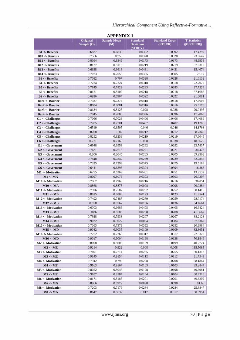
APPENDIX 1 Original

Sample (O)

Sample Mean

(M)

Standard

Deviation

(STDEV)

Standard Error

(STERR)

T Statistics

(|O/STERR|)

B1 <- Benefits 0.6837 0.6833 0.0392 0.0392 17.4292

B10 <- Benefits 0.7566 0.755 0.0328 0.0328 23.0647

B11 <- Benefits 0.8364 0.8345 0.0173 0.0173 48.3933

B12 <- Benefits 0.8127 0.8119 0.0219 0.0219 37.0319

B13 <- Benefits 0.6638 0.6618 0.0431 0.0431 15.4074

B14 <- Benefits 0.7073 0.7059 0.0305 0.0305 23.17

B3 <- Benefits 0.7082 0.707 0.0328 0.0328 21.6132

B4 <- Benefits 0.7224 0.7224 0.0318 0.0318 22.7072

B5 <- Benefits 0.7845 0.7822 0.0283 0.0283 27.7529

B6 <- Benefits 0.8121 0.8107 0.0218 0.0218 37.1688

B9 <- Benefits 0.6926 0.6904 0.0322 0.0322 21.5081

Bar1 <- Barrier 0.7387 0.7374 0.0418 0.0418 17.6608

Bar2 <- Barrier 0.8084 0.8081 0.0316 0.0316 25.6176

Bar3 <- Barrier 0.8134 0.8125 0.028 0.028 29.0495

Bar4 <- Barrier 0.7045 0.7085 0.0396 0.0396 17.7863

C1 <- Challenges 0.7066 0.7023 0.0406 0.0406 17.4086

C2 <- Challenges 0.7785 0.7701 0.0407 0.0407 19.1286

C3 <- Challenges 0.6519 0.6505 0.046 0.046 14.1763

C4 <- Challenges 0.8208 0.82 0.0212 0.0212 38.7346

C5 <- Challenges 0.8252 0.8258 0.0219 0.0219 37.6045

C6 <- Challenges 0.721 0.7169 0.038 0.038 18.9626

G1 <- Goverment 0.6948 0.6953 0.0292 0.0292 23.7837

G2 <- Goverment 0.7621 0.7618 0.0221 0.0221 34.473

G3 <- Goverment 0.806 0.8045 0.0205 0.0205 39.2363

G4 <- Goverment 0.7848 0.7842 0.0239 0.0239 32.7857

G5 <- Goverment 0.7325 0.7293 0.0375 0.0375 19.5188

G6 <- Goverment 0.6441 0.6396 0.0394 0.0394 16.363

M1 <- Motivation 0.6275 0.6269 0.0451 0.0451 13.9132

M1 <- MA 0.8097 0.8076 0.0303 0.0303 26.7307

M10 <- Motivation 0.7967 0.7969 0.0216 0.0216 36.851

M10 <- MA 0.8868 0.8875 0.0098 0.0098 90.0884

M11 <- Motivation 0.7596 0.7587 0.0252 0.0252 30.1415

M11 <- MB 0.8815 0.8803 0.0123 0.0123 71.9541

M12 <- Motivation 0.7492 0.7485 0.0259 0.0259 28.9174

M12 <- MB 0.878 0.8767 0.0136 0.0136 64.4664

M13 <- Motivation 0.6703 0.6688 0.0405 0.0405 16.5424

M13 <- MC 0.86 0.8585 0.0208 0.0208 41.3667

M14 <- Motivation 0.7928 0.7933 0.0207 0.0207 38.2123

M14 <- MC 0.9022 0.9027 0.0084 0.0084 107.6362

M15 <- Motivation 0.7363 0.7373 0.0352 0.0352 20.8984

M15 <- MD 0.9042 0.9035 0.0109 0.0109 82.8651

M16 <- Motivation 0.7272 0.7268 0.0317 0.0317 22.9329

M16 <- MD 0.9017 0.9004 0.0128 0.0128 70.1849

M2 <- Motivation 0.8008 0.8006 0.0199 0.0199 40.2724

M2 <- ME 0.9214 0.922 0.008 0.008 115.5085

M3 <- Motivation 0.7691 0.7714 0.0255 0.0255 30.1313

M3 <- ME 0.9145 0.9154 0.0112 0.0112 81.7542

M4 <- Motivation 0.7942 0.795 0.0208 0.0208 38.1864

M4 <- MF 0.9163 0.9164 0.0103 0.0103 89.2844

M5 <- Motivation 0.8052 0.8045 0.0198 0.0198 40.6981

M5 <- MF 0.9187 0.9184 0.0104 0.0104 88.4316

M6 <- Motivation 0.8171 0.8188 0.0201 0.0201 40.6202

M6 <- MG 0.8966 0.8972 0.0098 0.0098 91.66

M8 <- Motivation 0.7203 0.7179 0.0284 0.0284 25.3847

M8 <- MG 0.8647 0.8632 0.017 0.017 50.9954



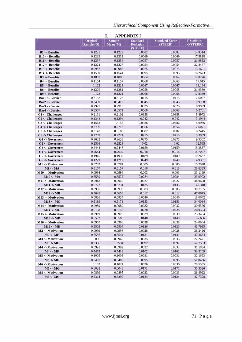
I. APPENDIX 2 Original

Sample (O)

Sample

Mean (M)

Standard

Deviation

(STDEV)

Standard Error

(STERR)

T Statistics

(|O/STERR|)

B1 <- Benefits 0.1221 0.1229 0.0082 0.0082 14.9314

B10 <- Benefits 0.1233 0.1232 0.0069 0.0069 17.8818

B11 <- Benefits 0.1257 0.1254 0.0057 0.0057 21.9852

B12 <- Benefits 0.1224 0.1227 0.0054 0.0054 22.8467

B13 <- Benefits 0.0987 0.0986 0.0075 0.0075 13.1601

B14 <- Benefits 0.1539 0.1541 0.0095 0.0095 16.2673

B3 <- Benefits 0.1087 0.1088 0.0064 0.0064 17.0276

B4 <- Benefits 0.1154 0.1157 0.0068 0.0068 17.015

B5 <- Benefits 0.122 0.1223 0.0067 0.0067 18.194

B6 <- Benefits 0.1279 0.1281 0.0058 0.0058 21.9589

B9 <- Benefits 0.122 0.1221 0.0068 0.0068 17.8339

Bar1 <- Barrier 0.3152 0.3123 0.0415 0.0415 7.6027

Bar2 <- Barrier 0.3439 0.3412 0.0345 0.0345 9.9738

Bar3 <- Barrier 0.2925 0.2913 0.0325 0.0325 8.9939

Bar4 <- Barrier 0.3567 0.3571 0.0568 0.0568 6.2781

C1 <- Challenges 0.2111 0.2102 0.0358 0.0358 5.8973

C2 <- Challenges 0.1343 0.1294 0.042 0.042 3.1944

C3 <- Challenges 0.1582 0.158 0.0386 0.0386 4.0936

C4 <- Challenges 0.2706 0.2718 0.0356 0.0356 7.6071

C5 <- Challenges 0.3147 0.3183 0.0382 0.0382 8.2445

C6 <- Challenges 0.2239 0.2221 0.0415 0.0415 5.3959

G1 <- Goverment 0.2622 0.2633 0.0275 0.0275 9.5362

G2 <- Goverment 0.2516 0.2528 0.02 0.02 12.565

G3 <- Goverment 0.2444 0.2448 0.0159 0.0159 15.3837

G4 <- Goverment 0.2644 0.2639 0.018 0.018 14.7057

G5 <- Goverment 0.1945 0.1937 0.0189 0.0189 10.2687

G6 <- Goverment 0.1229 0.1212 0.0249 0.0249 4.9331

M1 <- Motivation 0.0783 0.0781 0.005 0.005 15.7978

M1 <- MA 0.5167 0.5157 0.018 0.018 28.6383

M10 <- Motivation 0.0994 0.0994 0.003 0.003 33.1169

M10 <- MA 0.6559 0.6572 0.0284 0.0284 23.0902

M11 <- Motivation 0.0948 0.0946 0.0027 0.0027 34.9608

M11 <- MB 0.5722 0.5731 0.0135 0.0135 42.318

M12 <- Motivation 0.0935 0.0933 0.003 0.003 30.7185

M12 <- MB 0.5645 0.5653 0.012 0.012 47.0645

M13 <- Motivation 0.0836 0.0834 0.0046 0.0046 18.0642

M13 <- MC 0.5189 0.5178 0.0153 0.0153 34.0084

M14 <- Motivation 0.0989 0.0989 0.0032 0.0032 30.6576

M14 <- MC 0.6138 0.6152 0.0228 0.0228 26.9504

M15 <- Motivation 0.0919 0.0919 0.0039 0.0039 23.3464

M15 <- MD 0.5572 0.5583 0.0148 0.0148 37.656

M16 <- Motivation 0.0907 0.0906 0.0038 0.0038 24.0964

M16 <- MD 0.5503 0.5504 0.0126 0.0126 43.7935

M2 <- Motivation 0.0999 0.0998 0.0028 0.0028 36.2426

M2 <- ME 0.5556 0.5544 0.0131 0.0131 42.3634

M3 <- Motivation 0.096 0.0962 0.0035 0.0035 27.2471

M3 <- ME 0.5336 0.534 0.0092 0.0092 57.7553

M4 <- Motivation 0.0991 0.0992 0.0032 0.0032 31.1834

M4 <- MF 0.5412 0.5418 0.0102 0.0102 53.3109

M5 <- Motivation 0.1005 0.1003 0.0031 0.0031 32.1663

M5 <- MF 0.5487 0.5483 0.0095 0.0095 57.8436

M6 <- Motivation 0.102 0.1021 0.0036 0.0036 28.5535

M6 <- MG 0.6028 0.6048 0.0171 0.0171 35.3526

M8 <- Motivation 0.0899 0.0895 0.0033 0.0033 26.8922

M8 <- MG 0.5314 0.5299 0.0124 0.0124 42.7398

Hierarchical Component Using Reflective-Formative ......construct is namely Average Variance Extracted (AVE) proposed by Fornell & Larcker (1981). The formula of AVE is total factor

Documents