Guitar Tuner Project Report - EE 6th Sem

1 | P a g e

ABSTRACT:

In order to play beautiful music, a musician needs to have perfectly tuned instruments. If it is not

tuned properly, it will not sound good, even if you are playing everything correctly. As any novice

musician knows, one of the most frustrating parts of learning how to play guitar is tuning the

instrument which can be difficult for the untrained ear. This is where electronic tuners come in.

These small devices allow guitarists to perfectly tune their instruments.

The tuner is designed using the filtering, measuring and analyzing capabilities of the Arduino.

Compared to tuning by ear, where a certain amount of guess work is involved in deciding how much

to tighten/loosen a string, the Arduino based tuner is able to give accurate instructions so that tuning

can be achieved quicker.

2 | P a g e

ACKNOWLEDGEMENT:

On the very outset of this project, we would like to extend our sincere and heartfelt gratitude towards

our guide Mr. Shankar Banwasi for his constant support throughout the course of this venture.

We are ineffably indebted to Mrs Abha Tripathi for her conscientious guidance and encouragement

to accomplish this assignment.

We are extremely thankful and express our earnest gratitude to the faculty members of electrical and

electronics department of PESIT for providing us with valuable information in our endeavour.

We would also like to show our appreciation for our HOD Dr.B Keshavan and our principal Dr

K.N.B Murthy, for providing us with the opportunity to take this task upon ourselves.

3 | P a g e

TABLE OF CONTENTS

Chapter 1: Introduction

1.0: Electric Guitar Theory 4

1.1: Working of an Electric Guitar 5

Chapter 2: Design

2.0: Block Diagram Representation 6

2.1: Choice of Components and Cost Analysis

2.1.1: Op-Amp 6

2.1.2: Digital Signal Processing 7

2.1.3: LCD Display 7

2.2: External Circuit 8

2.3: Selection of Algorithm

2.3.1:Auto-Correlation 9

2.3.2:Measuring Zero Crossing with Positive Slope 10

Chapter 3: Implementation

3.0: External Circuit

3.0.1: Simulation Results 12

3.1: Implementation of Algorithm

3.1.1: Measuring Zero Crossing with Positive Slope 12

3.1.2: Auto-Correlation 13

3.2: Pitch Calculation 14

3.3: Output Display 15

3.4: Bread Board View 15

Chapter 4: Result and Conclusion 16

Chapter 5: Future Enhancements 17

Bibliography 18

Appendix

A1: Source code for Auto-Correlation 19

A2: Source Code for measuring Zero Crossing with Positive Slope 31

4 | P a g e

CHAPTER 1

INTRODUCTION

1.0 ELECTRIC GUITAR THEORY

A guitar is a six stringed musical instrument. It primarily consists of a neck and a body. The six

strings are strung along the neck to the bridge on the body. The thickness of each string is different.

Along the neck of the guitar are frets. Pressing the strings down onto the fret board changes the

length of the string, which changes the note being played. As the stings of the guitar are of a

particular length and tension, when played, each string corresponds to a particular note and thus can

be tuned to a particular note. Each musical note corresponds to a particular frequency of sound.

In western music there are 12 notes,

A A# B C C# D D# E F F# G G#

The set of these 12 notes make an octave.

Given below is the standard tuning of the guitar’s six strings along with the frequencies, from the

thickest to the thinnest string:

E: 82.41Hz

A: 110.00Hz

D: 146.83Hz

G: 196.00Hz

B: 246.94Hz

E: 329.63Hz

When the guitar goes out of tune, the frequency of the string does not correspond to that of the

expected note. A tuner detects the pitch of the notes played and gives visual feedback, to show how

far away the note is from the desired frequency.

A guitar note is not made up of a single frequency. It consists of a number of harmonics as well. The

difference in the harmonics is what makes a guitar and a violin sound different even while playing

the same note. Once a sample note is played on the guitar, its fundamental frequency has to be

calculated. A major part of the project is dedicated towards recovering the fundamental frequency

from the frequency spectrum of the sample note played on a guitar. Once recovered, it can be

compared with the standard to determine if the guitar is in tune.

5 | P a g e

1.1 WORKING OF AN ELECTRIC GUITAR

To produce sound, an electric guitar senses the vibrations of the strings electronically and routes an

electronic signal to an amplifier and speaker. The sensing occurs in electro- magnetic

pickup mounted under the strings on the guitar's body. The pickup consists of a bar magnet wrapped

with as many as 7,000 turns of fine wire. When the metal string is plucked, its vibration in the

pickup’s magnetic field induces a current in the wire of the pickup coil. This is determined by

Faraday’s law which states that, “any change in the magnetic environment of a coil of wire will

cause an emf to be induced in the coil.” The amplifier increases the electrical input’s amplitude and

the speaker then converts this to sound.

6 | P a g e

CHAPTER 2

DESIGN

2.0 BLOCK DIAGRAM REPRESENTATION

a) Amplifier stage

Amplifier stage contains a simple op-amp based audio amplifier, which amplifies the electrical

input obtained from the pickups

b) Analog to Digital converter

The ADC converts the analog input to a digital signal. The digital signal must have suitable

resolution and sampling frequency.

c) Digital Signal Processor

The DSP stage is used to estimate the fundamental frequency of the incoming signal using suitable

algorithms.

d) LCD Display

The LCD display is used to display how close the signal frequency is to the fixed standards. If the

signal frequency matches the standards exactly, the display reflects the note in tune. If the note is a

little too high or low relative to the fixed standards, the tuner will show the note as being little sharp

or flat respectively.

2.1 CHOICE OF COMPONENTS AND COST ANALYSIS

2.1.1 OP-AMP

We chose to use the TL072 (Texas Instruments IC) for the amplification stage. The low harmonic

distortion and low noise make the TL072 ideally suited for audio preamplifier applications.

7 | P a g e

2.1.2 DIGITAL SIGNAL PROCESSOR

The microcontroller is the ADC and DSP stage.

Our choice was between:

a) Arduino

b) MSP430 Launchpad

Parameters MSP430 Launchpad Arduino

Microcontroller TI M430G2553 ATMega328

Data Bus 16 bit 8 bit

Speed 16MHz 16Mhz

Storage 16KB 32KB

RAM 512B 2KB

Digital I/O 8 Channels 14 Channels

Analog I/O 8 Channels 6 Channels

IDE Code Composer Studio Arduino v1.0.1 IDE

Language Embedded C Arduino C

Kit Cost Rs.500 Rs.1200

Arduino is open source and its community support is unmatched compared to the Launchpad.

We chose the Arduino as it is easier to prototype on and it has larger RAM space compared to

the Launchpad; however the MSP430 is superior to the Arduino in terms of pricing and

versatility.

Thus as the aim was to prototype, we chose the Arduino. However if we intend to mass

produce our tuners, we would use the MSP430.

2.1.3 LCD DISPLAY

We use the D6711 7 segment LCD display, for displaying the note. 7 segment displays are used

to indicate decimal numerals or alphabets.

Once the guitar is tuned, the display will show the alphabet corresponding to the note being

played. If the frequency of the played note is too high or too low, this will be indicated by three

LED’s one to indicate the note is in tune, and the other two to indicate if the note is higher or

lower than the desired note.

8 | P a g e

2.2 EXTERNAL CIRCUIT

Ideally, the circuit would be the amplified output of the guitar connected to the arduino and the

arduino after determining the note, would show the required note on the display.

However, an audio signal, obtained from the amplifier shows two potential problems when fed

directly into the arduino’s analog input. The direct signal from the guitar is,

Of a very low peak to peak voltage (about 400mV)

Varies about the zero reference (whereas the Arduino’s analog input reads 0-5V)

Hence we must,

Amplify the audio signal to bring it to about 2.5V peak to peak

Provide a DC offset to the signal’s reference and make it fall within the 0-5V range.

The DC offset changes the reference voltage that the wave oscillates around, i.e. the average

voltage of the wave. Thus the reference voltage is brought to 2.5V and the amplified offset wave

oscillates between 0V and 5V.

We are using the following non-inverting amplifier configuration. Capacitor C3 is used to filter

out the high frequency noise. R4, R6 and C2 are used to provide a DC offset to the signal.

9 | P a g e

2.3 SELECTION OF ALGORITHM

2.3.1 AUTO-CORRELATION

Autocorrelation is a mathematical technique for the analysis of time series, or signal. It is exactly

the same as a cross correlation except, the same signal is correlated with itself. The basic

autocorrelation algorithm will now be presented, following which its application in finding the

fundamental frequency of the audio signal will be briefly illustrated.

Consider a discrete time signal xt and the integration window size is W. The Autocorrelation

function is defined as,

In the above equation, is the time lag of the second signal.

Consider a composite signal with most of its energy in one frequency, called the fundamental

frequency. It also contains a small fraction of the energy within the harmonics of that

fundamental frequency. This kind of a spectrum is native to most musical instrument sounds. The

timbre of the instrument is characterized by the specific levels of these harmonics and is usually

the result of the materials and physical characteristics of the instrument. Either way, the

fundamental frequency of the signal is the same regardless of what instrument is played.

Consider a composite signal like so.

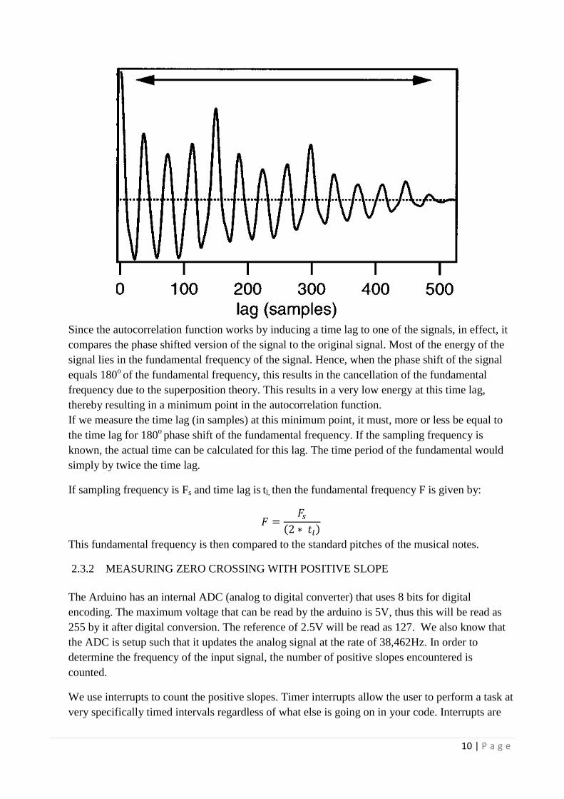
The magnitude of the autocorrelation function plot with respect to the time lag would result in a

graph like so.

10 | P a g e

Since the autocorrelation function works by inducing a time lag to one of the signals, in effect, it

compares the phase shifted version of the signal to the original signal. Most of the energy of the

signal lies in the fundamental frequency of the signal. Hence, when the phase shift of the signal

equals 180o of the fundamental frequency, this results in the cancellation of the fundamental

frequency due to the superposition theory. This results in a very low energy at this time lag,

thereby resulting in a minimum point in the autocorrelation function.

If we measure the time lag (in samples) at this minimum point, it must, more or less be equal to

the time lag for 180o phase shift of the fundamental frequency. If the sampling frequency is

known, the actual time can be calculated for this lag. The time period of the fundamental would

simply by twice the time lag.

If sampling frequency is Fs and time lag is tl, then the fundamental frequency F is given by:

This fundamental frequency is then compared to the standard pitches of the musical notes.

2.3.2 MEASURING ZERO CROSSING WITH POSITIVE SLOPE

The Arduino has an internal ADC (analog to digital converter) that uses 8 bits for digital

encoding. The maximum voltage that can be read by the arduino is 5V, thus this will be read as

255 by it after digital conversion. The reference of 2.5V will be read as 127. We also know that

the ADC is setup such that it updates the analog signal at the rate of 38,462Hz. In order to

determine the frequency of the input signal, the number of positive slopes encountered is

counted.

We use interrupts to count the positive slopes. Timer interrupts allow the user to perform a task at

very specifically timed intervals regardless of what else is going on in your code. Interrupts are

11 | P a g e

useful for measuring an incoming signal at equally spaced intervals at constant sampling

frequency.

The following figure should help illustrate this algorithm. The yellow signal is the audio signal.

The blue signal’s spikes indicate the time at which the audio signal crosses the reference with a

positive slope. The time between two consecutive spikes will give the time period of the

fundamental frequency.

12 | P a g e

CHAPTER 3

IMPLEMENTATION

3.0 EXTERNAL CIRCUIT

3.0.1 SIMULATION RESULTS

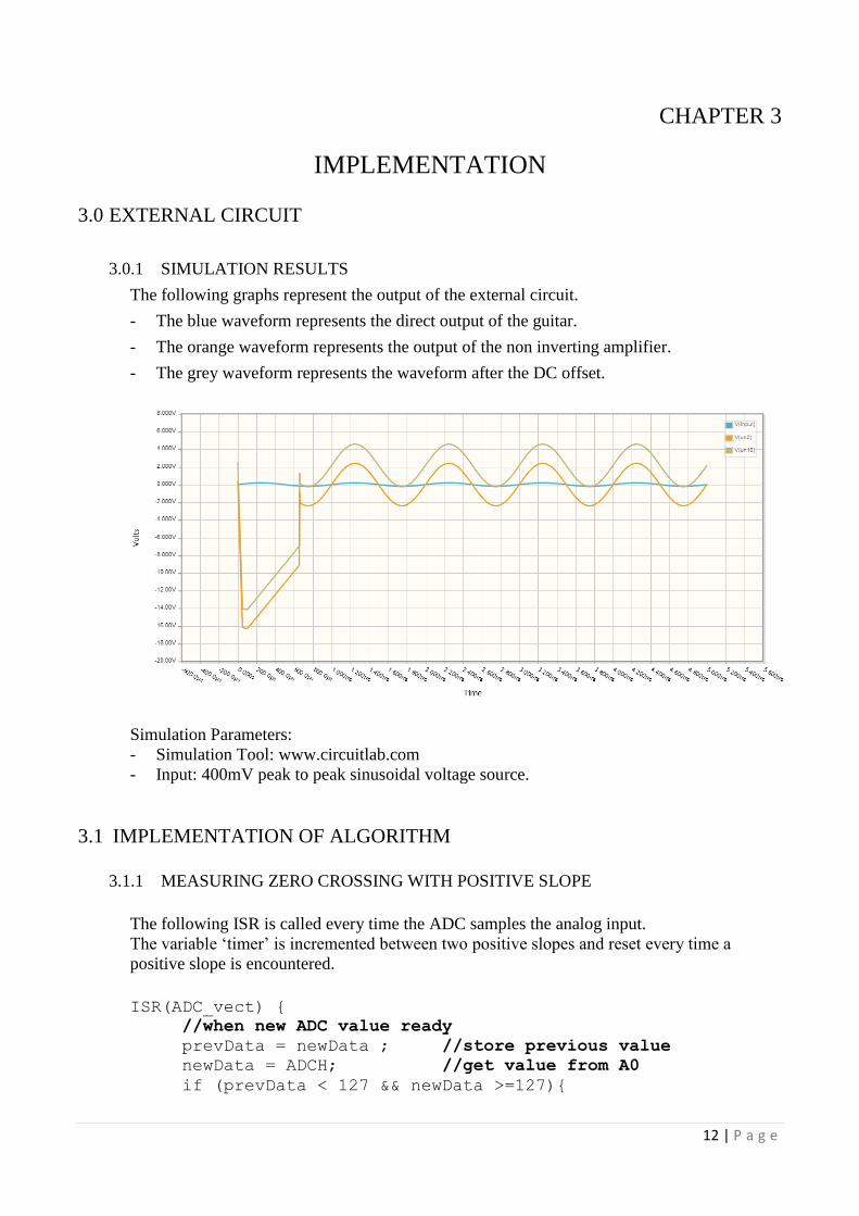
The following graphs represent the output of the external circuit.

- The blue waveform represents the direct output of the guitar.

- The orange waveform represents the output of the non inverting amplifier.

- The grey waveform represents the waveform after the DC offset.

Simulation Parameters:

- Simulation Tool: www.circuitlab.com

- Input: 400mV peak to peak sinusoidal voltage source.

3.1 IMPLEMENTATION OF ALGORITHM

3.1.1 MEASURING ZERO CROSSING WITH POSITIVE SLOPE

The following ISR is called every time the ADC samples the analog input.

The variable ‘timer’ is incremented between two positive slopes and reset every time a

positive slope is encountered.

ISR(ADC_vect) {

//when new ADC value ready

prevData = newData ; //store previous value

newData = ADCH; //get value from A0

if (prevData < 127 && newData >=127){

13 | P a g e

//if increasing and crossing midpoint

period = timer; //get period

timer = 0; //reset timer

}

timer++;

}

Since we know the sampling rate of the ADC, we can use it to calculate the fundamental

frequency using the following formula.

frequency = 38462/period;//timer-rate/period

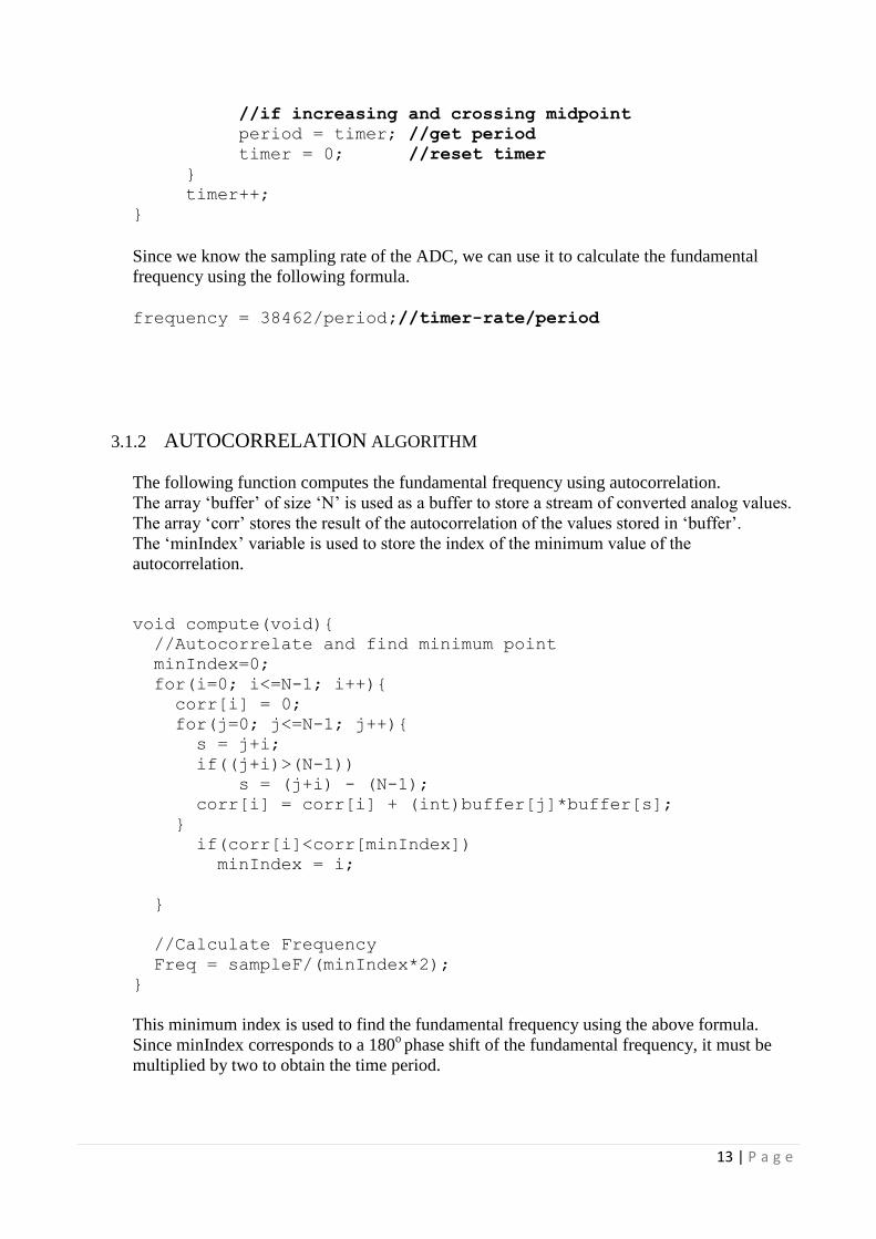
3.1.2 AUTOCORRELATION ALGORITHM

The following function computes the fundamental frequency using autocorrelation.

The array ‘buffer’ of size ‘N’ is used as a buffer to store a stream of converted analog values.

The array ‘corr’ stores the result of the autocorrelation of the values stored in ‘buffer’.

The ‘minIndex’ variable is used to store the index of the minimum value of the

autocorrelation.

void compute(void){

//Autocorrelate and find minimum point

minIndex=0;

for(i=0; i<=N-1; i++){

corr[i] = 0;

for(j=0; j<=N-1; j++){

s = j+i;

if((j+i)>(N-1))

s = (j+i) - (N-1);

corr[i] = corr[i] + (int)buffer[j]*buffer[s];

}

if(corr[i]<corr[minIndex])

minIndex = i;

}

//Calculate Frequency

Freq = sampleF/(minIndex*2);

}

This minimum index is used to find the fundamental frequency using the above formula.

Since minIndex corresponds to a 180o phase shift of the fundamental frequency, it must be

multiplied by two to obtain the time period.

14 | P a g e

3.2 PITCH CALUCLATION

We first store the standard frequencies of the notes of the lowest octave into their respective

variables in the following manner.

const int A = 110,

As = 116,

B = 123,

C = 131,

Cs = 139,

D = 147,

Ds = 156,

E = 165,

F = 171,

Fs = 185,

G = 196,

Gs = 208;

Now we decide which octave the incoming signal belongs to. The following code uses ‘Freq’

obtained from the frequency calculation algorithm. The variable ‘octave’ is later on used as a

multiplier while determining the pitch.

int octave = 1;

if(Freq > Gs*1)

octave = 2;

if(Freq > Gs*2)

octave =4;

if(Freq > Gs*4)

octave = 8;

The pitch is finally determined using the following ‘if-else’ construct. The variable ‘t’ determines the

tolerance band between which the frequency must lie in. At the centre of this tolerance band lies the

standard note frequency. If the input frequency lies within this tolerance band, it is assumed that the

end user intends to tune to that note.

if( Freq > (A*octave)*(1-t) && Freq < (A*octave)*(1+t) ){

note = A;

/*Signal the 7 seg display with the letter in each of

these if statements.*/

seven_seg_A();

}

This conditional is repeated for all of the notes.

15 | P a g e

3.3 OUTPUT DISPLAY

Output is displayed in the following manner:

- Green LED: Indicates the note is in tune.

- Red LED: Indicates the note out of tune and at a higher pitch.

- Blue LED: Indicates the note out of tune and at a lower pitch.

- Seven Segment Display: Displays the name of the note.

3.4 BREADBOARD VIEW

Following is a diagram of the breadboard view of our final circuit.

Software Used: Fritzing

16 | P a g e

CHAPTER 4

RESULT AND CONCLUSION

An accurate, real-time guitar tuner was constructed using an audio amplifier, an Arduino, an LCD

display and output LEDs. We tested two algorithms, zero crossing with positive slope and

autocorrelation.

We noticed that the zero crossing is fast and reasonably accurate. Although, it doesn’t work well

with increased noise levels and multiple zero crossings per cycle.

The autocorrelation algorithm computes the frequency by detecting the relative level of the

fundamental with respect to the other frequencies. This ensures accurate result even at very high

noise levels as the only requirement is that the maximum energy must be carried by the fundamental.

17 | P a g e

CHAPTER 5

FUTURE ENHANCEMENTS

This project can be extended to include automatic tuning of the guitar strings by using a motor to

turn the tuning pegs. These motors can be controlled by a voltage proportional to the amount of turn

required. We may estimate the frequency using the same algorithms.

We intended to implement the YIN algorithm [1] entirely but we used only the autocorrelation

portion of this algorithm as it sufficed our application. The YIN algorithm further uses a cumulative

mean normalized difference function along with parabolic interpolation to reduce the error by nearly

three times.

18 | P a g e

BIBILIOGRAPHY

[1] Alain de Cheveigne, Hideki Kawahara.

“YIN, a fundamental frequency estimator for speech and music”,

2002. Acoustical Society of America

[2] “Arduino Frequency Detection” by amandaghassaei

http://www.instructables.com/id/Arduino-Frequency-Detection/

[3] TL072 Datasheet

[4] D6711 Datasheet

http://www.instructables.com/id/Arduino-Frequency-Detection/

19 | P a g e

APPENDIX

A1. SOURCE CODE FOR AUTOCORRELATION ALGORITHM

/********************************************************************************

PESIT EEE 6th Sem Mini Project

May 2013

ELECTRONIC GUITAR TUNER

Tested on: Arduino Uno

Main Algorithm Used: Autocorrelation (for fundamental frequency)

Software version: 1.0.1

Test Parameters:

INPUT: Emulated Acoustic guitar sound from Guitar Pro V5 (for windows)

SIGNAL FLOW:

Computer Audio out->Operational Amplifier->Arduino Uno->7 Segment Display

USNs: 1PI10EE009

1PI10EE026

1PI10EE019

Source Code: http://pastebin.com/XiU7QHdk

********************************************************************************/

/*****************************************************************************

DECLARATIONS

******************************************************************************/

#define N 200 //Buffer Size

#define sampleF 38500//Hz

#define display_time 5000//ms

byte incomingAudio, bIndex=N-1;

int buffer[N];

long int corr[N], corrMin;

long int t_old, t_new = millis();

int i, j, minIndex,s;

int Freq=0;

boolean clipping = 0, flag = 0;

const int A = 110, //These are the standard note frequencies

As = 116, //At the lowest octave

B = 123,

C = 131,

Cs = 139,

D = 147,

Ds = 156,

E = 165,

F = 171,

Fs = 185,

G = 196,

Gs = 208;

int note = A;

int deviation = 0;

bool dev; //Higher or lower from the correct note

bool correct; //To show that the guitar is in tune

20 | P a g e

/*****************************************************************************

FUNCTION TO COMPUTE FUNDAMENTAL FREQUENCY

******************************************************************************/

void compute(void){

//Autocorrelate and find minimum point

minIndex=0;

for(i=0; i<=N-1; i++){

corr[i] = 0;

for(j=0; j<=N-1; j++){

s = j+i;

if((j+i)>(N-1))

s = (j+i) - (N-1);

corr[i] = corr[i] + (int)buffer[j]*buffer[s];

}

if(corr[i]<corr[minIndex])

minIndex = i;

}

//Calculate Frequency

Freq = sampleF/(minIndex*2);

}

/*****************************************************************************

PITCH DETECTION FUNCTION

******************************************************************************/

void pitch(void){

/*

This function is used to find the pitch after finding frequency and display

the

outputs on the 7 segment display and the LEDs

*/

const float t = 0.035; //tolerance band for note

const float t2 = 0.01; //tolerance band for correct note

int octave = 1;

//FIND OCTAVE

if(Freq > Gs*1)

octave = 2;

if(Freq > Gs*2)

octave =4;

if(Freq > Gs*4)

octave = 8;

/*FIND PITCH

The following portion is equivalent to checking if 'Freq'

lies within a certain band around the given note.

The width of this band is set by 't' (a percentage value)

Check if:

(input_note) lies within required_note +/-

(percentage*required_note)

*/


note = A;

21 | P a g e

//Signal the 7 seg display with the letter in each of these if

statements.

seven_seg_A();

}

else if( Freq > (As*octave)*(1-t) && Freq < (As*octave)*(1+t) ){

note = As;

seven_seg_As();

}

else if( Freq > (B*octave)*(1-t) && Freq < (B*octave)*(1+t) ){

note = B;

seven_seg_B();

}

else if( Freq > (C*octave)*(1-t) && Freq < (C*octave)*(1+t) ){

note = C;

seven_seg_C();

}

else if( Freq > (Cs*octave)*(1-t) && Freq < (Cs*octave)*(1+t) ){

note = Cs;

seven_seg_Cs();

}

else if( Freq > (D*octave)*(1-t) && Freq < (D*octave)*(1+t) ){

note = D;

seven_seg_D();

}

else if( Freq > (Ds*octave)*(1-t) && Freq < (Ds*octave)*(1+t) ){

note = Ds;

seven_seg_Ds();

}

else if( Freq > (E*octave)*(1-t) && Freq < (E*octave)*(1+t) ){

note = E;

seven_seg_E();

}

else if( Freq > (F*octave)*(1-t) && Freq < (F*octave)*(1+t) ){

note = F;

seven_seg_F();

}

else if( Freq > (Fs*octave)*(1-t) && Freq < (Fs*octave)*(1+t) ){

note = Fs;

seven_seg_Fs();

}

else if( Freq > (G*octave)*(1-t) && Freq < (G*octave)*(1+t) ){

note = G;

seven_seg_G();

}

else if( Freq > (Gs*octave)*(1-t) && Freq < (Gs*octave)*(1+t) ){

note = Gs;

seven_seg_Gs();

}

//DISPLAY

deviation = Freq - note*octave;

if (abs(deviation) < t2*note){

correct = 1; //in tune

//Serial.print(" ");

//Serial.println("Correct");

}

else{

correct = 0; //not in tune

if((deviation)>0){


//Serial.println("Note = deviated HIGH");

22 | P a g e

dev = HIGH;

}

else {

// Serial.print(" ");

//Serial.println("Deviated Low");

dev = LOW;

}

}

}

/***************END OF PITCH DETECTION FUNCTION****************/

/******************************************************************************

FUNCTIONS FOR 7 SEGMENT DISPLAY

*******************************************************************************/

//These are used to display the specific note on the 7 segment display

void seven_seg_A(void){

digitalWrite(9, LOW);



digitalWrite(6, HIGH);





if(correct == 1)

{

digitalWrite(12,LOW);

digitalWrite(11,HIGH);


}

else if(correct == 0)

{

if(dev == HIGH)

{




}

else if(dev == LOW)

{




}

}

}

void seven_seg_As(void){









if(correct == 1)

{


23 | P a g e



}


{

if(dev == HIGH)

{




}

else if(dev == LOW)

{




}

}

}

void seven_seg_B(void){









if(correct == 1)

{




}


{

if(dev == HIGH)

{




}

else if(dev == LOW)

{




}

}

}

void seven_seg_C(void){









24 | P a g e

if(correct == 1)

{




}


{

if(dev == HIGH)

{




}

else if(dev == LOW)

{




}

}

}

void seven_seg_Cs(void){









if(correct == 1)

{




}


{

if(dev == HIGH)

{




}

else if(dev == LOW)

{




}

}

}

void seven_seg_D(void){






25 | P a g e




if(correct == 1)

{




}


{

if(dev == HIGH)

{




}

else if(dev == LOW)

{




}

}

}

void seven_seg_Ds(void){









if(correct == 1)

{




}


{

if(dev == HIGH)

{




}

else if(dev == LOW)

{




}

}

}

void seven_seg_E(void){



26 | P a g e







if(correct == 1)

{




}


{

if(dev == HIGH)

{




}

else if(dev == LOW)

{




}

}

}

void seven_seg_F(void){









if(correct == 1)

{




}


{

if(dev == HIGH)

{




}

else if(dev == LOW)

{




}

}

}

27 | P a g e

void seven_seg_Fs(void){









if(correct == 1)

{




}


{

if(dev == HIGH)

{




}

else if(dev == LOW)

{




}

}

}

void seven_seg_G(void){









if(correct == 1)

{




}


{

if(dev == HIGH)

{




}

else if(dev == LOW)

{




}

28 | P a g e

}

}

void seven_seg_Gs(void){









if(correct == 1)

{




}


{

if(dev == HIGH)

{




}

else if(dev == LOW)

{




}

}

}

void blank(void){

//Blanks out the 7 Segment display












}

void test(void){

//To test the 7 Segment display

seven_seg_A();

delay(500);

seven_seg_As();

delay(500);

seven_seg_B();

delay(500);

seven_seg_C();

delay(500);

seven_seg_Cs();

29 | P a g e

delay(500);

seven_seg_D();

delay(500);

seven_seg_Ds();

delay(500);

seven_seg_E();

delay(500);

seven_seg_F();

delay(500);

seven_seg_Fs();

delay(500);

seven_seg_G();

delay(500);

seven_seg_Gs();

delay(500);

blank();

}

/***************END OF 7 SEG FUNCTIONS****************/

/*****************************************************************************

SETUP

******************************************************************************/

void setup(){

pinMode(13,OUTPUT);//led clipping indicator pin

cli(); //disable interrupts

//set up continuous sampling of analog pin 0

ADCSRA = 0; //clear ADCSRA and ADCSRB registers

ADCSRB = 0;

ADMUX |= (1 << REFS0); //set reference voltage

ADMUX |= (1 << ADLAR); //left align the ADC value- so we can read highest 8

bits from ADCH register only

ADCSRA |= (1 << ADPS2) | (1 << ADPS0); //set ADC clock with 32 prescaler-

16mHz/32=500kHz

//ADCSRA |= (1 << ADPS2) | (0 << ADPS1) | (0 << ADPS0);

ADCSRA |= (1 << ADATE); //enabble auto trigger

ADCSRA |= (1 << ADIE); //enable interrupts when measurement complete

ADCSRA |= (1 << ADEN); //enable ADC

ADCSRA |= (1 << ADSC); //start ADC measurements

sei();//enable interrupts

Serial.begin(9600);

}

/*****************************************************************************

INTERRUPT SERVICE ROUTINE

******************************************************************************/

ISR(ADC_vect) {//when new ADC value ready

incomingAudio = ADCH;//store 8 bit value from analog pin 0

//t_new = millis();

if (incomingAudio == 0 || incomingAudio == 255){//if clipping

digitalWrite(13,HIGH);//set pin 13 high

clipping = 1;//currently clipping

}

//Store in buffer //Works

30 | P a g e

if(bIndex!=N-1){

buffer[bIndex] = incomingAudio;

bIndex++;

}

else{

bIndex = 0;

//flag = 1;

}

}

/***************END OF INTERRUPT SERVICE ROUTINE**************/

/*****************************************************************************

LOOP

******************************************************************************/

void loop(){

if (clipping){//if currently clipping

clipping = 0;//

digitalWrite(13,LOW);//turn off clipping led indicator (pin 13)

}

cli();

compute();

//To print results on serial monitor

//Serial.print(Freq);

//Serial.println(" hz");

sei();

}

/***************END OF LOOP**************/

31 | P a g e

A2. SOURCE CODE FOR ZERO CROSSING WITH POSITIVE SLOPE ALGORITHM

/*****************************************************************************

PESIT EEE 6th Sem Mini Project

May 2013

ELECTRONIC GUITAR TUNER

Tested on: Arduino Uno

Main Algorithm Used: Slope detection (for fundamental frequency)

Software version: 1.0.1

Test Parameters:

INPUT: Emulated Acoustic guitar sound from Guitar Pro V5 (for windows)

SIGNAL FLOW:

Computer Audio out->Operational Amplifier->Arduino Uno->7 Segment Display

USNs: 1PI10EE009

1PI10EE026

1PI10EE019

Source Code: http://pastebin.com/mS1y9FhC

*****************************************************************************/

/*****************************************************************************

DECLARATIONS

******************************************************************************

/

byte incomingAudio;

int Freq=0;

boolean clipping = 0, flag = 0;

const int A = 110, //These are the standard note frequencies

As = 116, //At the lowest octave

B = 123,

C = 131,

Cs = 139,

D = 147,

Ds = 156,

E = 165,

F = 171,

Fs = 185,

G = 196,

Gs = 208;

int note = A;

int deviation = 0;

bool dev; //Higher or lower from the correct note

bool correct; //To show that the guitar is in tune

//data storage variables

byte newData = 0;

byte prevData = 0;

unsigned int time = 0; //keeps time and sends vales to store in timer[]

occasionally

int timer[10]; //sstorage for timing of events

int slope[10]; //storage for slope of events

unsigned int totalTimer;//used to calculate period

32 | P a g e

unsigned int period; //storage for period of wave

byte index = 0; //current storage index

float frequency; //storage for frequency calculations

int maxSlope = 0; //used to calculate max slope as trigger point

int newSlope; //storage for incoming slope data

//variables for decided whether you have a match

byte noMatch = 0; //counts how many non-matches you've received to reset

variables if it's been too long

byte slopeTol = 3; //slope tolerance- adjust this if you need

int timerTol = 10; //timer tolerance- adjust this if you need

//variables for amp detection

unsigned int ampTimer = 0;

byte maxAmp = 0;

byte checkMaxAmp;

byte ampThreshold = 30; //raise if you have a very noisy signal

/***************END OF INITIAL DECLARATIONS****************/

/*****************************************************************************

PITCH DETECTION FUNCTION

******************************************************************************

/

void pitch(void){

/*

This function is used to find the pitch after finding frequency and display

the

outputs on the 7 segment display and the LEDs

*/

const float t = 0.035; //tolerance band for note

const float t2 = 0.01; //tolerance band for correct note

int octave = 1;

//FIND OCTAVE

if(Freq > Gs*1){


//Serial.print("Once Octave");

octave = 2;}

if(Freq > Gs*2){


//Serial.print("twice Octave");

octave =4;}

if(Freq > Gs*4)

octave = 8;

/*FIND PITCH

The following portion is equivalent to checking if 'Freq'

lies within a certain band around the given note.

The width of this band is set by 't' (a percentage value)

Check if:

(input_note) lies within required_note +/-

(percentage*required_note)

*/


note = A;

//Signal the 7 seg display with the letter in each of these if

statements.

33 | P a g e

seven_seg_A();

}

else if( Freq > (As*octave)*(1-t) && Freq < (As*octave)*(1+t) ){

note = As;

seven_seg_As();

}

else if( Freq > (B*octave)*(1-t) && Freq < (B*octave)*(1+t) ){

note = B;

seven_seg_B();

}

else if( Freq > (C*octave)*(1-t) && Freq < (C*octave)*(1+t) ){

note = C;

seven_seg_C();

}

else if( Freq > (Cs*octave)*(1-t) && Freq < (Cs*octave)*(1+t) ){

note = Cs;

seven_seg_Cs();

}

else if( Freq > (D*octave)*(1-t) && Freq < (D*octave)*(1+t) ){

note = D;

seven_seg_D();

}

else if( Freq > (Ds*octave)*(1-t) && Freq < (Ds*octave)*(1+t) ){

note = Ds;

seven_seg_Ds();

}

else if( Freq > (E*octave)*(1-t) && Freq < (E*octave)*(1+t) ){

note = E;

seven_seg_E();

}

else if( Freq > (F*octave)*(1-t) && Freq < (F*octave)*(1+t) ){

note = F;

seven_seg_F();

}

else if( Freq > (Fs*octave)*(1-t) && Freq < (Fs*octave)*(1+t) ){

note = Fs;

seven_seg_Fs();

}

else if( Freq > (G*octave)*(1-t) && Freq < (G*octave)*(1+t) ){

note = G;

seven_seg_G();

}

else if( Freq > (Gs*octave)*(1-t) && Freq < (Gs*octave)*(1+t) ){

note = Gs;

seven_seg_Gs();

}

//DISPLAY

deviation = Freq - note*octave;

if (abs(deviation) < t2*note){

correct = 1; //in tune


//Serial.println("Correct");

}

else{

correct = 0; //not in tune

if((deviation)>0){


//Serial.println("Note = deviated HIGH");

dev = HIGH;

}

34 | P a g e

else {

// Serial.print(" ");

//Serial.println("Deviated Low");

dev = LOW;

}

}

}

/***************END OF PITCH DETECTION FUNCTION****************/

/*****************************************************************************

*

FUNCTIONS FOR 7 SEGMENT DISPLAY

******************************************************************************

*/

//These are used to display the specific note on the 7 segment display

void seven_seg_A(void){









if(correct == 1)

{




}


{

if(dev == HIGH)

{




}

else if(dev == LOW)

{




}

}

}

void seven_seg_As(void){









if(correct == 1)

{


35 | P a g e



}


{

if(dev == HIGH)

{




}

else if(dev == LOW)

{




}

}

}

void seven_seg_B(void){









if(correct == 1)

{




}


{

if(dev == HIGH)

{




}

else if(dev == LOW)

{




}

}

}

void seven_seg_C(void){









36 | P a g e

if(correct == 1)

{




}


{

if(dev == HIGH)

{




}

else if(dev == LOW)

{




}

}

}

void seven_seg_Cs(void){









if(correct == 1)

{




}


{

if(dev == HIGH)

{




}

else if(dev == LOW)

{




}

}

}

void seven_seg_D(void){






37 | P a g e




if(correct == 1)

{




}


{

if(dev == HIGH)

{




}

else if(dev == LOW)

{




}

}

}

void seven_seg_Ds(void){









if(correct == 1)

{




}


{

if(dev == HIGH)

{




}

else if(dev == LOW)

{




}

}

}

void seven_seg_E(void){



38 | P a g e







if(correct == 1)

{




}


{

if(dev == HIGH)

{




}

else if(dev == LOW)

{




}

}

}

void seven_seg_F(void){









if(correct == 1)

{




}


{

if(dev == HIGH)

{




}

else if(dev == LOW)

{




}

}

}

39 | P a g e

void seven_seg_Fs(void){









if(correct == 1)

{




}


{

if(dev == HIGH)

{




}

else if(dev == LOW)

{




}

}

}

void seven_seg_G(void){









if(correct == 1)

{




}


{

if(dev == HIGH)

{




}

else if(dev == LOW)

{




}

40 | P a g e

}

}

void seven_seg_Gs(void){









if(correct == 1)

{




}


{

if(dev == HIGH)

{




}

else if(dev == LOW)

{




}

}

}

void blank(void){

//Blanks out the 7 Segment display












}

void test(void){

//To test the 7 Segment display

seven_seg_A();

delay(500);

seven_seg_As();

delay(500);

seven_seg_B();

delay(500);

seven_seg_C();

delay(500);

seven_seg_Cs();

41 | P a g e

delay(500);

seven_seg_D();

delay(500);

seven_seg_Ds();

delay(500);

seven_seg_E();

delay(500);

seven_seg_F();

delay(500);

seven_seg_Fs();

delay(500);

seven_seg_G();

delay(500);

seven_seg_Gs();

delay(500);

blank();

}

/***************END OF 7 SEG FUNCTIONS****************/

/*****************************************************************************

INTERRUPT SERVICE ROUTINE

******************************************************************************

/

ISR(ADC_vect) {//when new ADC value ready

PORTB &= B11101111;//set pin 12 low

prevData = newData;//store previous value

newData = ADCH;//get value from A0

if (prevData < 127 && newData >=127){//if increasing and crossing midpoint

newSlope = newData - prevData;//calculate slope

if (abs(newSlope-maxSlope)<slopeTol){//if slopes are ==

//record new data and reset time

slope[index] = newSlope;

timer[index] = time;

time = 0;

if (index == 0){//new max slope just reset

PORTB |= B00010000;//set pin 12 high

noMatch = 0;

index++;//increment index

}

else if (abs(timer[0]-timer[index])<timerTol && abs(slope[0]-

newSlope)<slopeTol){//if timer duration and slopes match

//sum timer values

totalTimer = 0;

for (byte i=0;i<index;i++){

totalTimer+=timer[i];

}

period = totalTimer;//set period

//reset new zero index values to compare with

timer[0] = timer[index];

slope[0] = slope[index];

index = 1;//set index to 1

PORTB |= B00010000;//set pin 12 high

noMatch = 0;

}

else{//crossing midpoint but not match

index++;//increment index

if (index > 9){

reset();

}

42 | P a g e

}

}

else if (newSlope>maxSlope){//if new slope is much larger than max slope

maxSlope = newSlope;

time = 0;//reset clock

noMatch = 0;

index = 0;//reset index

}

else{//slope not steep enough

noMatch++;//increment no match counter

if (noMatch>9){

reset();

}

}

}

if (newData == 0 || newData == 1023){//if clipping

PORTB |= B00100000;//set pin 13 high- turn on clipping indicator led

clipping = 1;//currently clipping

}

time++;//increment timer at rate of 38.5kHz

ampTimer++;//increment amplitude timer

if (abs(127-ADCH)>maxAmp){

maxAmp = abs(127-ADCH);

}

if (ampTimer==1000){

ampTimer = 0;

checkMaxAmp = maxAmp;

maxAmp = 0;

}

}

void reset(){//clea out some variables

index = 0;//reset index

noMatch = 0;//reset match couner

maxSlope = 0;//reset slope

}

void checkClipping(){//manage clipping indicator LED

if (clipping){//if currently clipping

PORTB &= B11011111;//turn off clipping indicator led

clipping = 0;

}

}

/***************END OF INTERRUPT SERVICE ROUTINE**************/

/*****************************************************************************

SETUP

******************************************************************************

/

void setup(){

Serial.begin(9600);

pinMode(13,OUTPUT);//led indicator pin

43 | P a g e

pinMode(12,OUTPUT);//output pin

cli();//diable interrupts

//set up continuous sampling of analog pin 0 at 38.5kHz

//clear ADCSRA and ADCSRB registers

ADCSRA = 0;

ADCSRB = 0;

ADMUX |= (1 << REFS0); //set reference voltage

ADMUX |= (1 << ADLAR); //left align the ADC value- so we can read highest 8

bits from ADCH register only

ADCSRA |= (1 << ADPS2) | (1 << ADPS0); //set ADC clock with 32 prescaler-

16mHz/32=500kHz

ADCSRA |= (1 << ADATE); //enabble auto trigger

ADCSRA |= (1 << ADIE); //enable interrupts when measurement complete

ADCSRA |= (1 << ADEN); //enable ADC

ADCSRA |= (1 << ADSC); //start ADC measurements

sei();//enable interrupts

pinMode(13,OUTPUT);//led indicator pin

pinMode(12, OUTPUT);



pinMode(9, OUTPUT);

pinMode(8, OUTPUT);

pinMode(7, OUTPUT);

pinMode(6, OUTPUT);

pinMode(5, OUTPUT);

pinMode(4, OUTPUT);

pinMode(3, OUTPUT);

pinMode(2, OUTPUT);

blank();

//test();

}

/***************END OF SETUP**************/

/*****************************************************************************

LOOP

******************************************************************************

/

void loop(){

checkClipping();

if (checkMaxAmp>ampThreshold){

//calculate frequency timer rate/period

Freq = 38462/float(period);

//To print results on serial monitor

//Serial.print(Freq);

//Serial.println(" hz");

}

//Detect and display the pitch

pitch();

}

44 | P a g e

/***************END OF LOOP**************/

Guitar Tuner Project Report - EE 6th Sem

Documents