GSTAR MODELS WITH ARCH ERRORS AND THE SIMULATIONS

1075

GSTAR MODELS WITH ARCH ERRORS AND THE SIMULATIONS

Nelson Nainggolan1), Budi Nurani Ruchjana2), Sutawanir Darwis3), Rustam E. Siregar4)

1)A lecturer at the Department of Mathematics, Universitas Sam Ratulangi -Indonesia

2)A lecturer at the Department of Mathematics, Universitas Padjadjaran-Indonesia 3)A lecturer at the Mathematics Study Program, Institut Teknologi Bandung-

Indonesia 4) A lecturer at the Department of Fhysics, Universitas Padjadjaran-Indonesia

Email: [email protected]

Abstract. Generalisasi Space Time Autoregressive (GSTAR) models was introduced in Ruchjana (2002) assumed constant variance errors. In this paper, we consider GSTAR models with ARCH errors (GSTAR-ARCH), the mean equation was GSTAR models and the variance equations is modelled by the ARCH models. The conditional variance of errors conditions on the past changed over time but the unconditional variance was constant. The error terms as a multivariat ARCH is

modeled by constant conditional correlations models. The least squared method used to estimated the mean equation (GSTAR) parameters then the error term (ARCH) parameters estimated by maximum likelihood method. We apply the GSTAR-ARCH model using simulation data. The simulation results shows that the proposed method works well in estimating the model parameters.

Keywords: GSTAR, arch, conditional variance

1 Introduction GSTAR models are often useful in modeling time series involved time variable and

space-time variable. However, these model have the assumption of homoscedastic (or equal variance) for the errors. This is not appropriate when dealing with the financial market variables such as the stock price indices or currency exchange rates. In the real situation we often find that the variance changes over all time t. The financial market variables typically have characteristics which the assumption of homoscedastic have failed to consider. These typical are the unconditional distribution of financial time series has heavier tails than the normal distribution, Values of t do not have much correlation, but values of t2 are highly correlated

and the changes in t tend to cluster, large (or small) changes in t tend to be

followed by large (or small) changes. So that, in the financial market variables the assumption of heteroscedastic more appropriate. One of the time series models allowing for heteroscedasticity is the Autoregressive Conditional Heteroscedastic (ARCH) model introduced by Engle (1982).

In this paper, we will study about the orde-1 GSTAR-ARCH model. The estimation of parameters concist of two parts, the least squared method used to estimate the

Proceedings of the Third International Conference on Mathematics and Natural Sciences (ICMNS 2010)

Nelson Nainggolan, Budi Nurani Ruchjana, Sutawanir Darwis, Rustam E. Siregar

1076

mean equation (GSTAR) parameters then the error term (ARCH) parameters are estimated using maximum likelihood method. The objectives of this paper are (1) To introduce the GSTAR-ARCH Models, (2) To study the parameter estimation of the order-1 GSTAR-ARCH model and (3) To give an illustration about the GSTAR-ARCH model.

2. ARCH Models

Suppose 1 2, , , T are the time series observation and let tF be the set of

t up to time t, including t for .0t The process { t } is an Autoregressive

Conditional Heteroscedastic process of order-q, ARCH(q), if statisfy

1 ~ (0, )t t tF N h (1)

2 2

0 1 1t t q t qh (2)

wiht q > 0, α0 > 0, and αi ≥ 0, for i = 1, 2, ……., q. From (1),

1( ) 0t tE F

2

1 1( ) ( )t t t t tVar F E F h .

Next, the process {t} is a Generalized Autoregressive Conditional Heteroscedastic

process of order p and q, GARCH(p,q), if :

1 ~ (0, )t t tF N h

2 2

0 1 1 1t t q t q j t p t ph h h (3)

where q > 0, α0 > 0, and αi ≥ 0, for i = 1, 2, ……., q, ,0j for j = 1, 2, ……., p.

Next, deviding by the square root of the conditional variance of Xt from (1), we have:

1 ~ (0,1)t t th F N

and therefore the sequence 1 , …… , T , defined by t t th

t t th (4)

should be independent and identically distributed i.i.d. N(0,1). So, the ARCH process {t} can be constructed from a sequence of i.i.d N(0,1) random variables.

In general, the time series models can be written in the form

( , 1)t t tZ f X t (5)

where Zt : time series at the time t, f(Xt, t-1) : mean equations, t : variance (innovation) equations of the error.

Next, Consider (5) and let the mean equations is ordinary regression models and the variance equations is ARCH models It is called regression-ARCH models (Engle, 1982). The regression-ARCH(q) models can be written as

1 ~ ( , )t t tZ F N h tX β

Zt = Xt + εt (6)

GSTAR Models with ARCH Errors and the Simulations

1077

ttt h

22

110 qtqtth (7)

where 0 0, 0, 1, ,i i q , t ~ iid. N(0,1).

The specific of regression-ARCH models is that the errors staisfy the ARCH process. In this models, Xt may include lagged dependent and exogenous variables. The ordinary least squares (OLS) estimator of is still consistent as X and are

uncorrelated throught the difinition of the regression as a conditional expectation. The procedures to estimate the parameters, rare first, estimate by OLS and then

obtain the residuals. From these residuals, estimate the parameters in (7),

0 1ˆ ( , , , )p , and based on these ̂ , efficient estimated of are found (see:

Engle, 1982).

2 Results and Discussion

Let (1), (2), , ( )Tz z z are the time series observations. The process {z(t)} with

1( ) ( ( ), , ( ))Nt Z t Z t z

is an order-1 Generalized Space Time Autoregressive models, GSTAR(1,1), that is order-1 at lag-time and order-1 at lag-spacial, if statisfy

10 11( ) ( 1) ( 1) ( )t t t t z Φ z Φ Wz ε

10 11( ) ( 1) ( )t t t z I W z ε

( ) ( 1) ( )t t t z z ε (8)

where 2( ) (0, )~iid

Nt N ε I

10 11 I W

W is weight matrix. The assumption for in (8), the error variance are constant every time (homoscedasticity). To estimates the parameters of these models, make the models in linear form

Y = X + ε (9)

where 2(0, )~iid

T NN ε I . The least square estimation of the parameters used the

formula (Ruchjana, 2002):

1ˆ ( ) β X X X Y (10)

Let, the errors in (8) have not constan conditional variance but change over time

(heteroscedasticity), follows the ARCH process. Thus, the models have the mean equations as a GSTAR models and the errors as the multivariat ARCH models. This model called GSTAR-ARCH models. The assumption of heteroscedastic for the errors in (9), conditional on the full matrix X, then

2~ (0, )N ε V

where V is diagonal matrix, V = diag(h1, h2, ... , hNT),


1078

hi is the i component conditional variance of . For more detail, see Hamilton

(1994). The estimation parameters of the GSTAR models in heteroscedastic assumption is estimated by generalized least square (GLS) method. The GLS estimation is

1 1 1ˆ ( ) β X V X X V Y (11)

For example, the orde-1 GSTAR-ARCH models that is the mean equations as a

GSTAR(1,1) models and the errors as the multivariat ARCH(1) models. Let

1 2( ) ( ( ), ( )) 't Z t Z tz

1 2( ) ( ( ), ( )) 't t t ε ,

then the orde-1 GSTAR-ARCH models for two locations with uniform weigt matrix W is

1( ) ( 1) ( )t t t z z ε (12)

1( ) ~ (0, )t tt F Nε H

where

1 10 11 I W

11 21

1

21 22

( ) ( )( ( ) )

( ) ( )t t

h t h tVar t F

h t h t

ε H . (13)

In this paper, we consider the multivariate ARCH models for Ht is the constant conditional correlation (CCC) models (Bollerslev, 1990). The CCC model for the ARCH multivariate models of Ht two locations, written as

Ht = DtR Dt where

1 2( ( ) , ( ))t diag h t h tD

R = [ij] was correlation between i,t and j,t , ( ) ( ) 2

0 1( ) ( )i i

ii ih t t

( ) ( ) ( )ij ij ii jjh t h t h t , for i, j = 1,2.

Analog with the uivariat ARCH models, we can write the error terms as

( ) t tt ε D η

where 1 2( ( ), ( )) 't t t η is a vektor of i.i.d. random variable sequence, zerro mean

and covariance matrix 2

N I . Hence, to make data simulation first generate the

random variable sequences, 1(t) and 2(t), zerro mean and one variance. Then,

generate error terms

1 2( ) ( ( ), ( )) 't t t ε ,

where 1 1 1( ) ( ) ( )t h t t ,

2 2 2( ) ( ) ( )t h t t , and h1(t), h2(t) are the ARCH in (2).

The matrix form of (11) in two locations is

(1) (1)1 1 1 110 11

(2) (2)2 2 2 210 11

( ) ( 1) ( 1) ( )0 10 0

( ) ( 1) ( 1) ( )1 00 0

Z t Z t Z t e t

Z t Z t Z t e t

.

The GSTAR-ARCH models in the linear form (9) is Y = X + ε


1079

where

1 1 2 2(1) ( ) (1) ( )Z Z T Z Z T Y

(1) (2) (1) (2)

10 10 11 11

β

1 1

1 1

1 1

2 2

2 2

2 2

(0) 0 (0) 0

(1) 0 (1) 0

( 1) 0 ( 1) 0

0 (0) 0 (0)

0 (1) 0 (1)

0 ( 1) 0 ( 1)

z V

z V

z T V T

z V

z V

z T V T

X

and

( ) ( )i ij j

j i

V t w Z t

, for i, j = 1, 2; t = 0, 1, ... , T-1.

[ ]ijwW is the weight matrix.

The simulation data of GSTAR(1,1)-ARCH(1) models for two locations

In this section, we simulated the data for T = 100. First, generated 100 data, the

errors of the order-1 GSTAR-ARCH models, 1(t) and 2(t). The conditional variance of the errors are respectively:

2

11 1( ) 0.05 0.82 ( 1)h t t

2

22 2( ) 0.15 0.78 ( 1)h t t

Then, generated the GSTAR(1,1) models for 2 lokations, Z(t) = (Z1(t), Z2(t)) , where

the errors is 1 1( ) ( ( ), ( ))t t t ε . The simulations of GSTAR models are given

parameter values (1) (2)

10 100.38, 0.42

(1) (2)

11 110.31, 0.27 .

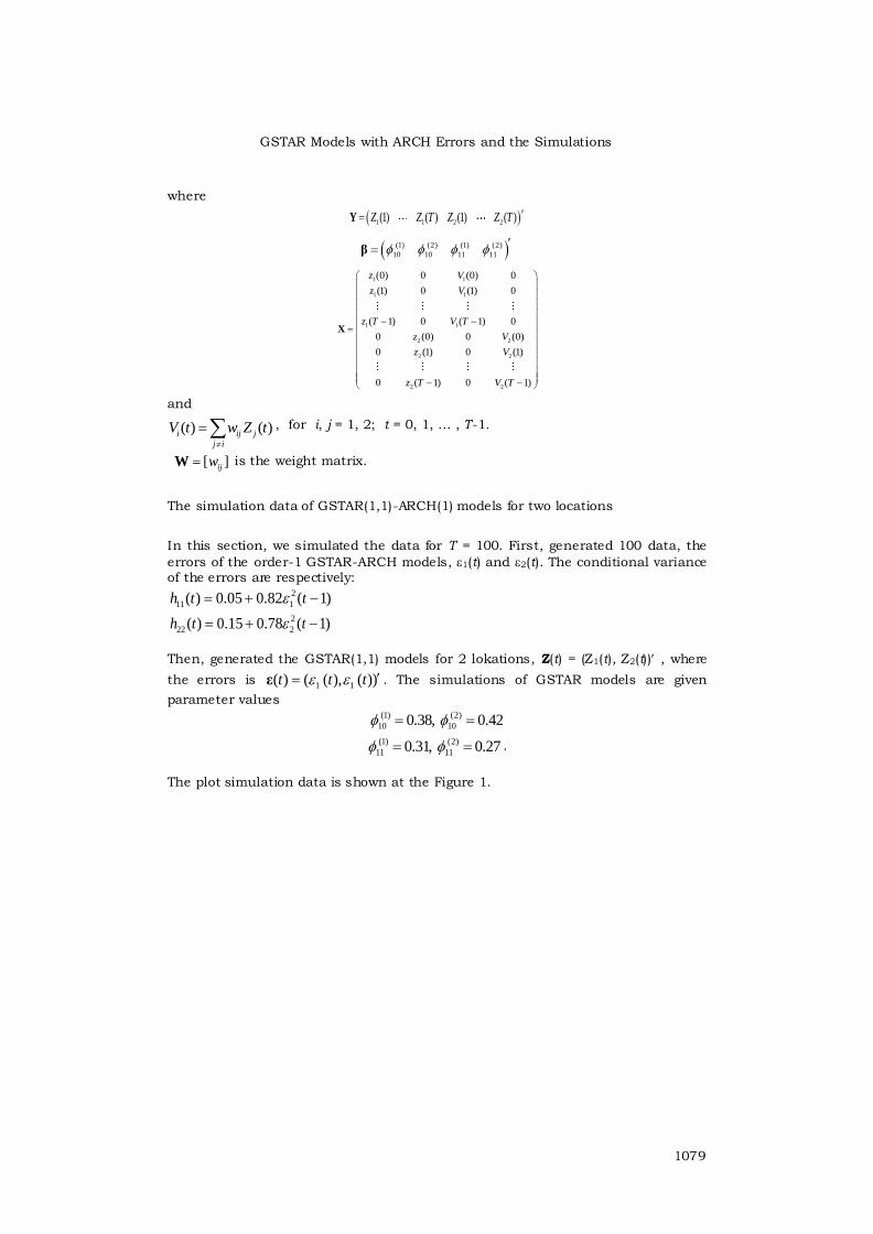
The plot simulation data is shown at the Figure 1.


1080

Plot z1(t) Data Simulation

w ak tu

z(t)

0 20 40 60 80 100

-10

1

Plot z2(t) Data Simulation

w ak tu

z(t)

0 20 40 60 80 100

-2-1

01

Figure 1. Plot Data Simulations T = 100 of GSTAR(1,1)-ARCH(1) Models. The

parameters are (1) (2)

10 100.38, 0.42 , (1) (2)

11 110.31, 0.27 .

Next, we want to know, how the arch effect toward the simulation data. The test of effect acrh for Z1(t) and Z2(t), by Splus+Finmetrics, we obtain p-value: 0.0023, 0.6184, respectively. So that, the arch effect to the simulation data Z1(t) was significant at the level 95%. It’s mean that the data have non constant conditional variance. Hence, the simulation data can be modelled by GSTAR models with the error ARCH models. To estimate the parameters of the GSTAR(1,1) models, first, assume that the variance are constant, then the parameter estimaions of the models in the linear

form (9), using the formula (10). By the Splus programme, we get > ParGstArch.pred1 [,1] [1,] 0.1055615 [2,] 0.3914703 [3,] 0.5113156 [4,] 0.2207569

The Least Square Estimating (LSE) β̂ are (1)

10 0.1056 , (2)

10 0.3915 , (1)

11 0.5113 ,

(2)

11 0.2208 . Used this parameters, then we compute the prediction ( )

ˆ ( )i LSZ t and

then the residuals

( )ˆ( ) ( ) ( )i i i LSe t Z t Z t , i = 1, 2, .

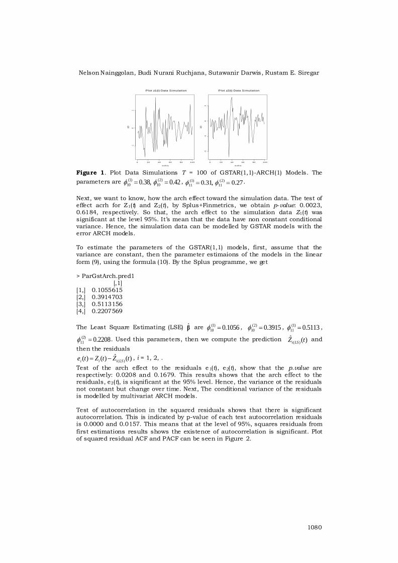
Test of the arch effect to the residuals e1(t), e2(t), show that the p.value are respectively: 0.0208 and 0.1679. This results shows that the arch effect to the residuals, e2(t), is siqnificant at the 95% level. Hence, the variance ot the residuals not constant but change over time. Next, The conditional variance of the residuals is modelled by multivariat ARCH models. Test of autocorrelation in the squared residuals shows that there is significant autocorrelation. This is indicated by p-value of each test autocorrelation residuals is 0.0000 and 0.0157. This means that at the level of 95%, squares residuals from

first estimations results shows the existence of autocorrelation is significant. Plot of squared residual ACF and PACF can be seen in Figure 2.


1081

LagA

CF

0 5 10 15 20-0

.20

.20

.61

.0

ACF e1(t) 2̂

Lag

AC

F

0 5 10 15 20

-0.2

0.2

0.6

1.0

ACF e2(t) 2̂

Lag

Pa

rtia

l AC

F

0 5 10 15 20

-0.2

0.0

0.2

0.4

PACF e1(t) 2̂

Lag

Pa

rtia

l AC

F

0 5 10 15 20

-0.2

0.0

0.1

0.2

0.3

PACF e2(t) 2̂

Figure 2. Plot ACF and PACF of residual square on the first estimations. There is autocorrelation on the residuals squares. The PACF cuts the significant line at the lag-2 on the e1(t)^2 and lag-1 on the e2(t)2.

From the arch effect test, autoorrelation test and the plot ACF, PACF of residuals squares, then the conditional variance or the error was eligible if it is modeled with arch models. The conditional variance CCC models by splus program are > e12pred1.ts.ccc = mgarch(e12pred1.ts~1, ~ccc(1,0), trace=F) > e12pred1.ts.ccc Call: mgarch(formula.mean = e12pred1.ts ~ 1, formula.var = ~ ccc(1, 0), trace = F) Coefficients: C(1) -0.01228 C(2) -0.03643

A(1, 1) 0.10172 A(2, 2) 0.04519 ARCH(1; 1, 1) 0.58228 ARCH(1; 2, 2) 0.73171 Conditional Constant Correlation Matrix: 1.1 1.00000 -0.08968 1.2 -0.08968 1.00000 Therefore, the CCC models for conditional variance Ht of (13) are

2

11 1

2

22 2

( ) 0.10172 0.58228 ( 1)

( ) 0.04519 0.73171 ( 1)

h t t

h t t

(14)

and the conditional covariances are

21 11 22( ) 0.08968 ( ) ( )h t h t h t

From (14), compute the conditional variance h11(t) and h22(t) for t = 2, 3, ... , T, and collect all in the matriks diagonal V2(T-1), where

11 11 22 22( (2), , ( ), (2), , ( ))diag h h T h h TV (15)


1082

The second stage of the parameter estimations for mean equations is GLS estimator by using conditional variance (15). The estimation results with S-Plus are > Parmtr.gstarArch.GLS [,1] [1,] 0.2593025 [2,] 0.3302879 [3,] 0.4027038 [4,] 0.1720437

Hence, the inprovement parameter are

(1) (2)

10 10

(1) (2)

11 11

ˆ 0.2593, 0.3303

ˆ ˆ0.4027, 0.17204

Thus, the mean prediction models, GSTAR(1,1), of the data simulation two locations are

1 1 2

2 2 2

ˆ ( ) 0,2593 ( 1) 0,4027 ( 1)

ˆ ( ) 0,3303 ( 1) 0,17204 ( 1)

Z t Z t Z t

Z t Z t Z t

We use this parameters, then compute the prediction ( )

ˆ ( )i LSZ t . The GLS residuals

are

ˆˆ ( ) ( ) ( )i i it Z t Z t , i = 1, 2.

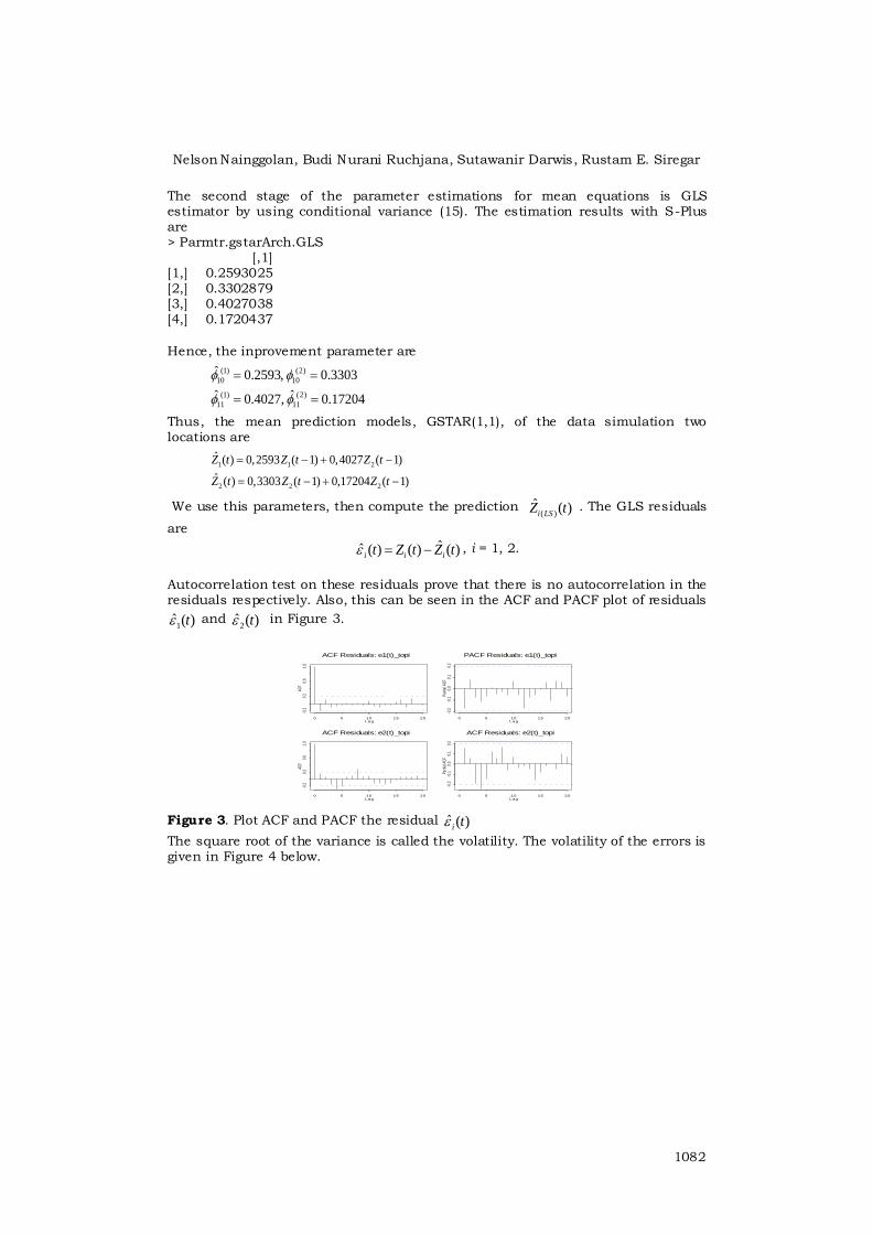
Autocorrelation test on these residuals prove that there is no autocorrelation in the residuals respectively. Also, this can be seen in the ACF and PACF plot of residuals

1ˆ ( )t and

2ˆ ( )t in Figure 3.

Lag

ACF

0 5 10 15 20

-0.2

0.2

0.6

1.0

ACF Residuals: e1(t)_topi

Lag

Parti

al A

CF

0 5 10 15 20

-0.2

-0.1

0.0

0.1

0.2

PACF Residuals: e1(t)_topi

Lag

ACF

0 5 10 15 20

-0.2

0.2

0.6

1.0


Lag

Parti

al A

CF

0 5 10 15 20

-0.2

-0.1

0.0

0.1

0.2


Figure 3. Plot ACF and PACF the residual ˆ ( )i t

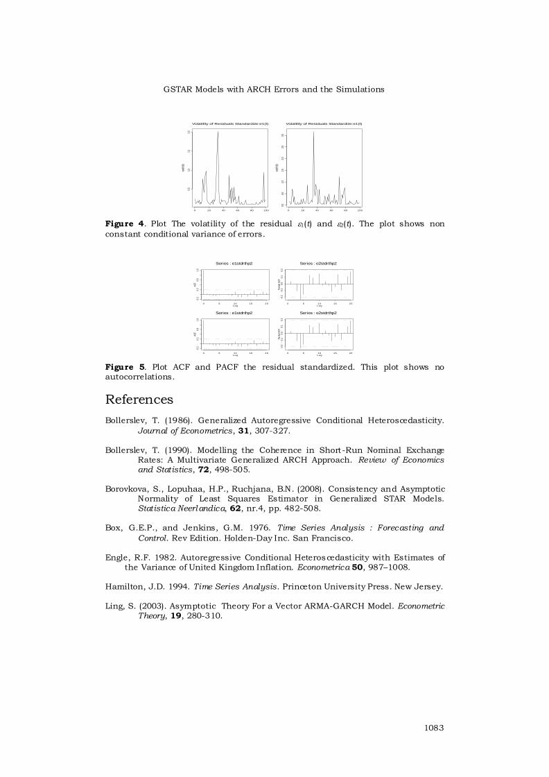
The square root of the variance is called the volatility. The volatility of the errors is given in Figure 4 below.


1083

Figure 4. Plot The volatility of the residual 1(t) and 2(t). The plot shows non

constant conditional variance of errors.

Lag

AC

F

0 5 10 15 20

-0.2

0.2

0.6

1.0

Series : e1stdrthp2

Lag

Pa

rtia

l AC

F

0 5 10 15 20

-0.2

-0.1

0.0

0.1

0.2

Series : e2stdrthp2

Lag

AC

F

0 5 10 15 20

-0.2

0.2

0.6

1.0

Series : e1stdrthp2

Lag

Pa

rtia

l AC

F

0 5 10 15 20

-0.2

-0.1

0.0

0.1

0.2

Series : e2stdrthp2

Figure 5. Plot ACF and PACF the residual standardized. This plot shows no autocorrelations.

References Bollerslev, T. (1986). Generalized Autoregressive Conditional Heteroscedasticity.

Journal of Econometrics, 31, 307-327. Bollerslev, T. (1990). Modelling the Coherence in Short-Run Nominal Exchange

Rates: A Multivariate Generalized ARCH Approach. Review of Economics and Statistics, 72, 498-505.

Borovkova, S., Lopuhaa, H.P., Ruchjana, B.N. (2008). Consistency and Asymptotic

Normality of Least Squares Estimator in Generalized STAR Models. Statistica Neerlandica, 62, nr.4, pp. 482-508.

Box, G.E.P., and Jenkins, G.M. 1976. Time Series Analysis : Forecasting and

Control. Rev Edition. Holden-Day Inc. San Francisco. Engle, R.F. 1982. Autoregressive Conditional Heteroscedasticity with Estimates of

the Variance of United Kingdom Inflation. Econometrica 50, 987–1008. Hamilton, J.D. 1994. Time Series Analysis. Princeton University Press. New Jersey. Ling, S. (2003). Asymptotic Theory For a Vector ARMA-GARCH Model. Econometric

Theory, 19, 280-310.

Volatility of Residuals Standardize:e1(t)

sqrt{

h(t)}

0 20 40 60 80 100

0.5

1.0

1.5

2.0

Volatility of Residuals Standardize:e1(t)

sqrt{

h(t)}

0 20 40 60 80 100

0.0

0.5

1.0

1.5

2.0

2.5

3.0


1084

Ruchjana, B.N. (2002). Suatu Model Generalisasi Space-Time Autoregresi dan Penerapannya pada Produksi Minyak Bumi. (Disertasi) Institut Teknologi Bandung.

Tsay, R. S. University of Chicago. (2002). Analysis Financial Time Series. Financial

Econometrics. John Wiley & Sons, Inc. USA. Wei, W.W.S. 1990. Time Series Analysis : Univariate and Multivariate Models .

Addison-Wesley Publishing Company, Inc. USA. Zivot, E. and Wang, J. (2006). Modelling Financial Time Series with S-PLUS. 2nd

ed. Springer Science+Business Media, LLC. USA. http://seldon.it.northwestern.edu/sscc/splus/finmetrics.pdf, 3 september 2010 .

http://seldon.it.northwestern.edu/sscc/splus/finmetrics.pdf

GSTAR MODELS WITH ARCH ERRORS AND THE SIMULATIONS

Documents