GEOTECHNICAL LARGE DEFORM ATION NUMERICAL ANALYSIS … · GEOTECHNICAL LARGE DEFORM ATION NUMERICAL ANALYSIS USING IMPLICIT AND EXPLICIT INTEGRATION Montaser BAKROON1, Daniel AUBRAM2,Frank

3rd International Conference on New Advances in Civil Engineering APRIL 28-29, 2017, HELSINKI, FINLAND

26

GEOTECHNICAL LARGE DEFORMATION NUMERICAL ANALYSIS USING IMPLICIT AND EXPLICIT INTEGRATION

Montaser BAKROON1, Daniel AUBRAM2,Frank RACKWITZ3

1Technische Universität Berlin (TU Berlin), Secr. TIB1-B7, Gustav-Meyer-Allee 25, D-13355 Berlin, Germany, [email protected]

2TU Berlin, Secr.TIB1-B7, Gustav-Meyer-Allee 25, D-13355 Berlin, Germany, [email protected] 3TU Berlin, Secr. TIB1-B7, Gustav-Meyer-Allee 25, D-13355 Berlin, Germany, [email protected]

Abstract 1. The dynamic analysis of a non-linear large deformation Geotechnical problems using the standard Lagrange finite element method (FEM) can experience numerical difficulties. These difficulties as contact problems, convergence and large mesh deformations can stop the simulation process. Moreover, the extremely non-linear behavior of the soil material consequently involves non-convergence issues. This paper addresses the application of different FEM formulations (implicit Lagrange, explicit Lagrange, and Coupled Eulerian-Lagrangian (CEL)) methods, to non-linear dynamic large deformation. The explicit dynamic FEM solves equations without iterations in contrast to implicit methods which involves iterations to satisfy a convergence at each increment, that leads to a time/CPU consuming solution. Implicit and explicit FEM generally implement different procedures to update the stress and state variables of a material in the computational model. In this contribution a user subroutine for granular soil material behavior is developed based on hypoplasticity which implemented in the ABAQUS/explicit package. Accordingly, the explicit user subroutine version is verified by comparing the results with implicit version utilizing basic element tests (Oedometer and Triaxial tests). This paper also investigates the CEL analysis method which is developed to overcome the limitation of implicit and Lagrange explicit methods. However, CEL formulation overcomes the problem of large deformations of the mesh and the contact problems and thereby facilitates the convergence in dealing with a highly non-linear material behavior. Two example applications of the hypoplastic material in conjunction with the implicit Lagrange, explicit Lagrange and CEL methods are presented. The first example is a strip footing problem which uses Tresca model to investigate and compare between the previous numerical analysis methods. The second example simulates a single pile penetration into a subsoil, this test shows that the user subroutine hypoplastic model is acceptable for modelling granular material. By comparing the results, it is concluded that the CEL method using hypoplastic soil material is suitable for large deformation Geotechnical problems. Key Words: Coupled Eulerian-Lagrangian, Hypoplasticity, Large deformations, Oedometer and Triaxial tests, Pile jacking

Introduction Soil-structure interaction and in particular large deformations in geotechnical engineering are considered as

important problems to be studied. However, analysis of this interaction faces many challenges, and the large soil deformations need special techniques for numerical simulation. Large deformations may cause severe distortion of the computational mesh, which may stop the analysis in early stages. Consequently, several variants of the Finite Element Method (FEM) have been developed to overcome these problems[1, 2]. Among these, the Arbitrary Lagrangian-Eulerian (ALE), Multi-Material ALE (MMALE), and Coupled Eulerian-Lagrangian (CEL) methods overcome the disadvantages of the classical Lagrangian approach in solid mechanics while showing good agreement with experimental results.

During the last decade, CEL [3–5] and other approaches [6–8] became popular for solving geotechnical problems. Qiu and Henke [9], for example, applied CEL to a strip footing, an anchor plate problem, and other applications. They conclude that the CEL method is most suitable for the geotechnical applications involving very large soil deformations. In this paper, the CEL method will be combined with a sophisticated constitutive equation for the soil and compared to other computational models for reasons of verification and validation, and in order to expand the range of application of this particular method.

Simulations of geotechnical problems often require fine mesh models and advanced constitutive equations for the soil. However, the increase of mesh elements in conjunction with non-linear soil models leads to a time/CPU consuming solution. This calls for efficient numerical methods that often use explicit algorithms to advance the solution in time. A special soil material model called “hypoplasticity” will be used in the simulations. The available hypoplasticity subroutine is in a form that can be used with implicit numerical methods. Therefore, one objective of the present research is to reformulate this implicit subroutine to be applicable with the explicit methods.

The explicit user subroutine version is verified by comparing the results with implicit version utilizing basic element tests (Oedometer and Triaxial tests). Three example applications of the hypoplastic material in conjunction with the implicit Lagrange, explicit Lagrange and CEL methods will be presented. The first example is a strip footing problem which uses Tresca model to investigate and compare between the previous numerical analysis methods. The second example is a pile penetration problem using hypoplastic soil material which investigated and compared to experimental results, this test shows that the user subroutine hypoplastic model is acceptable for modelling granular material.


27

Coupled Eulerian-Lagrangian (CEL) method In the pure Lagrangian method, the mesh nodes are associated with material particles. That means when the

material deforms the mesh will deform in accordance. Unfortunately, the large distortion of the mesh will stop the simulation. On the other hand, the Eulerian method allows the material to flow through the mesh elements and that enables the simulation to continue with existence of large deformations. The CEL method captures the strengths of Lagrangian and Eulerian methods as shown in fig. 1.

Fig. 1: FE model Initial configuration (left), Material deformation in a Lagrangian analysis (middle) and a Coupled Eulerian-Lagrangian

analysis (right).

The CEL method treats the penetrator as (Pile, Spudcan, or any structural element) as the Lagrangian part, while the soil treated as Eulerian part. The Lagrangian part can move freely through the Eulerian mesh until it encounters a Eulerian material. The latter situation is then treated by a penalty contact formulation. The penalty method applies springs between material interfaces to resist additional penetration. These springs have seeds which are created on the Lagrangian element edges and faces and anchor points which are created on the Eulerian material surface. The spring forces are governed by this equation where is the spring force and is the distance of peneteriaon which is proprotional to the penetration distance .

The CEL method implementation is based on the Eulerian volume fraction (EVF) approach. The material is tracked as it flows through the mesh by computing and advecting its EVF within each element. When a Eulerian element is completely filled with a material, EVF=1; if there is no material in the element, EVF=0, and a EVF in between indicates that the material boundary (or interface) crosses the element.In each time step there are two sub phases. The first is a Lagrangian phase which the element deforms with the material, and the second is a Eulerian phase which relocates the mesh to its original position and then remaps the material distribution and solution variables from the old onto the relocated mesh.

It is good to notice that in order to minimize the time of calculation without affecting the performance of the simulation, a deformation tolerance is applied not to deform elements with minor deformation.

Implicit/Explicit theoretical background

The implicit solution method depends on the state of the FE model at the time point under study[10, 11]. In other words, if the FE model is updated from then the equilibrium will be satisfied for this sate at time

, while the explicit solution method will satisfy the equilibrium at time depends on the data of the model at time .

The explicit solution method has the advantage to minimize the processing time and memory requirements [12]. Many more advantages have the explicit solution method over the Implicit solution method for large deformations in geotechnical problems. The computational time in the explicit method is linearly proportional to model size, while in the implicit method the time increases quadratically with the model size as will be discussed in the equations below.

The stability limit of the explicit method is bounded by a maximum time increment, which must be less than the speed of sound to cross the smallest element size of the model. This limitation is excluded from the implicit scheme and it solves the dynamic quantities at time based not only on the information at time but also at time . Implicit scheme gives acceptable, accurate results for the same models solved by explicit scheme using time increments 10 or 100 times the time increments used in explicit scheme, but the response prediction will deteriorate as the time step size, , increases relative to the period, T, of typical modes of response. The implementation of large deformations, contact constraints, and sliding are very easy in the explicit method. Implicit solution method:

The implicit method uses a backward Euler operator[13], which updates the FE model from t to ∆t+1 then the equilibrium will be satisfied for this sate at time ∆t+1, while the explicit solution method will satisfy the equilibrium at time ∆t+1 depends on the data of the model at time t. That means the explicit solution method has the advantage to minimize the processing time and memory requirements. The explicit dynamic FEM solves equations without iterations in contrast to implicit methods which involves iterations to satisfy a convergence at


28

each increment, that leads to a time/CPU consuming solution. Implicit and explicit FEM generally implement different procedures to update the stress and state variables of a material in the computational model.

The time integration of the dynamic problem uses the operator defined by Hilber, Hughes, and Taylor [14]. Which is used to control the numerical damping. The implicit procedure uses suitable root finding technique of a full Newton-Raphson solution method[15]:

Where is the current tangent stiffness matrix, F the applied load vector, I the internal force vector, is the

increment of displacement, and is the time step. For as implicit method, the algorithm is defined by [15]:

Where M is the mass matrix, K the stiffness matrix, F the vector of applied loads and u the displacement vector:

and

where is velocity and is acceleration. with

where are the integration parameters. For certain values of and the integration scheme can be

rendered unconditionally stable. The parameter is chosen by default in Abaqus as a small damping term to avoid numerical noise [15].

Explicit solution method:

The explicit dynamics method is based on the application of an explicit time integration rule with the use of diagonal mass matrices for the elements. The central difference scheme is applied to the equations of motions of the body:

The superscript refer to the increment value and mid-increment values, respectively.

By knowing the values of and from previous increment, the central difference operator is explicit in that the kinematic state can be advanced [15].

The explicit method is simple and does not require iterations or a tangent stiffness matrix. In order to further increase computational efficiency, the element mass matrix is “lumped” to become diagonal. This leads to an inexpensive matrix inversion in Eq. (8).

The value of the time increment has to be limited by:

where is the maximum element eigen value. A practical method to implement the above limit is:


29

where is the characteristic minimum element length in the model, is the dilatational wave speed, and can be calculated by the following equation:

where and are the Lamé elastic constants and is the material density. In a quasi-static analysis, the time

increment used for an explicit scheme is much smaller than with the implicit scheme for an equivalent problem. The sizes of the elements should be regular in order to obtain efficient analysis results. Otherwise, a single element may increase the time of the analysis for the whole model [16].

In a quasi-static analysis, it is impractical to run the model with its real time scale, as it will be very large. There are a number of ways to overcome this issue. A mass scale is one of a used style practice. According to the equations (10) and (11), the time increment is proportional to the square root of the density. That is, if the density increased by a factor the time will be reduced by . However, the changes must not increase the internal forces in order not to alter the solution.

In the quasi-static simulation, controlling the internal forces has an important rule. The internal forces must not affect the mechanical response in order not to produce increase values for the internal forces which is not real. Kutt et al. [11] recommend that the internal energy should not increase more than 5% of the kinetic energy. So that the dynamic effects will be reduced and can be neglected.

Hypoplasticity subroutine validation Constitutive model description

This study investigates the penetration into non-cohesive, granular materials like sand. Due to the limitations of the failure criteria for typical material models implemented in commercial software, and to get a realistic description of the granular soil material behavior, the constitutive equation implemented here is the hypoplastic model by von Wolffersdorff in 1996[17]. The intergranular strain extension proposed by Niemunis and Herle [18] captures the accumulative effects and the hysteretic material behavior under cyclic loading.

Hypoplasticity suits well the nonlinear and non-elastic behavior of granular materials. The constitutive model simulates some of the main interesting soil properties like dilatancy and contractancy, depending on stress state and void ratio[19].Accordingly, the dependency on the void ratio of the soil allows for realistic simulation of compaction processes. A user hypoplastic material subroutine for explicit analysis was developed in this study relying on an implicit version which was implemented by Nuebel and Niemunis[20].

The hypoplastic constitutive model of von Wolffersdorff takes the form [21]:

where denotes the co-rotational Jaumann stress rate, is the strain rate tensor, is a fourth-order tensor

associated with the linear part of the behavior and is a second-order tensor related to the nonlinear part of the behavior. The mathematical representation of and is:

where


30

In order to take into account the effects of the accumulation of deformation behavior under cyclic loading, an intergranular strain extension has been made by Niemunis and Herle [18]. The constitutive model is formulated as a rate independent by tensorial function:

Where is the objective Jaumann stress rate, the strain rate and a fourth order tensor, this tensor depends

on the void ratio and the intergranular strain .

The Oedometer test For reasons of verification a comparison has been carried out between the implemented explicit version of the

hypoplastic material subroutine and the implicit version already available[17, 18]. The schematic diagram of the finite element model used for the oedometer test is illustrated in Fig.2. The material parameters used in the numerical simulations are depicted in Table 1. The initial void ratio used is 0 and the applied load is

.

Table 1. Hypoplastic parameters of Hochstetten sand. c [°] s [MPa] d0 c0 i0 por0 33 1000 0.25 0.55 0.95 1.05 0.25 1 0.695 5.0 2.0 1x10-4 6.0 0.5

Fig.2. (a) schematic diagram illustrating an Oedometer test; (b) FE-mesh and boundary conditions

It is clear that the implemented explicit version of the hypoplastic user material (Abaqus Explicit VUMAT

subroutine) is in good acceptance with the reference model of the implicit version (Abaqus Standard UMAT subroutine) as shown in Fig. 3. In the left plot the intergranular strain was deactivated and in the right plot the intergranular strain was activated.

Fig. 3. Void ratio – Stress curve for oedometric compression test (a) the intergranular strain deactivated; (b)the intergranular strain activated

The Triaxial test:

In the Triaxial test a one element model illustrated in Fig. 4 was applied. The same material parameters as in the oedometer test (Table 1) were used. The initial void ratio used is 0 with initial isotropic load

, and the applied load was .


31

Fig. 4. (a) Schematic diagram illustrating an triaxial test (left), FE-mesh and boundary conditions (right).

Fig. 5 shows that the void ratio vs stress curve is in good correlation to the reference model [17, 18].

Fig. 5. Void ratio – Stress for Triaxial compression test with intergranular strain.

Numerical examples Strip footing problem

The strip footing is a problem where material deformations are large and a closed-form analytical solution is available. Three computational models using different numerical analysis methods are compared: implicit Lagrange FEM, explicit Lagrange FEM, and the explicit Coupled Eulerian-Lagrangian method. The results of the pressure under the footing will be compared to the analytical solution done by Hill [22]. Hill processed a billet which held in a container and hollowed out by punch. He regarded the problem as a plane strain problem in order to simplify the solution. The container is smooth, so the sides of the material will be fixed only in the horizontal direction and the bottom face will be fixed in the vertical direction. The punch assumed as a rigid body with no relative displacement base and smooth sides.

Fig. 6: Geometry and boundary conditions for strip footing problem

For the ratio of base over soil width = 0.5, the maximum punch pressure for this problem is (Hill 1950)[22] where in this model is the soil shear strength.


32

The soil material parameters used in the problem are shown in table 2, where c is the soil cohesion, is poison ratio and is the modulus of elasticity. The Tresca constitutive model is adopted.

Table 2. Material parameters for the soil.

[kPa] [kPa] [-] 2980 10 0.49

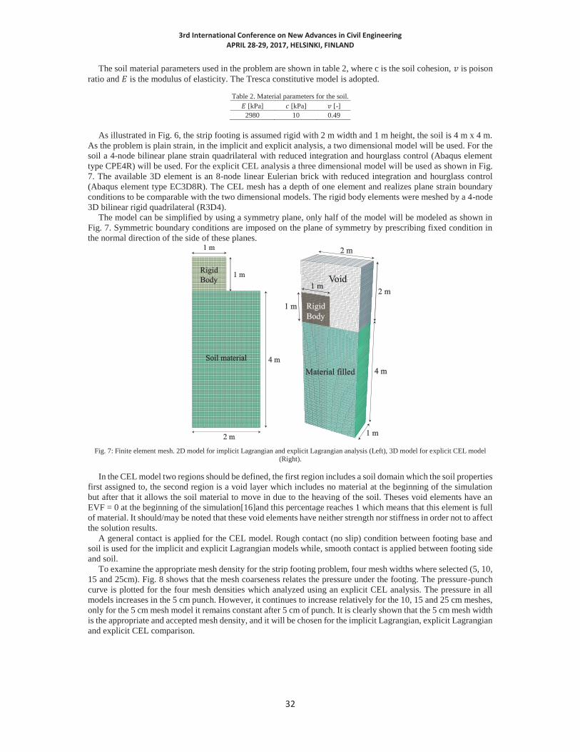
As illustrated in Fig. 6, the strip footing is assumed rigid with 2 m width and 1 m height, the soil is 4 m x 4 m.

As the problem is plain strain, in the implicit and explicit analysis, a two dimensional model will be used. For the soil a 4-node bilinear plane strain quadrilateral with reduced integration and hourglass control (Abaqus element type CPE4R) will be used. For the explicit CEL analysis a three dimensional model will be used as shown in Fig. 7. The available 3D element is an 8-node linear Eulerian brick with reduced integration and hourglass control (Abaqus element type EC3D8R). The CEL mesh has a depth of one element and realizes plane strain boundary conditions to be comparable with the two dimensional models. The rigid body elements were meshed by a 4-node 3D bilinear rigid quadrilateral (R3D4).

The model can be simplified by using a symmetry plane, only half of the model will be modeled as shown in Fig. 7. Symmetric boundary conditions are imposed on the plane of symmetry by prescribing fixed condition in the normal direction of the side of these planes.

Fig. 7: Finite element mesh. 2D model for implicit Lagrangian and explicit Lagrangian analysis (Left), 3D model for explicit CEL model

(Right).

In the CEL model two regions should be defined, the first region includes a soil domain which the soil properties first assigned to, the second region is a void layer which includes no material at the beginning of the simulation but after that it allows the soil material to move in due to the heaving of the soil. Theses void elements have an EVF = 0 at the beginning of the simulation[16]and this percentage reaches 1 which means that this element is full of material. It should/may be noted that these void elements have neither strength nor stiffness in order not to affect the solution results.

A general contact is applied for the CEL model. Rough contact (no slip) condition between footing base and soil is used for the implicit and explicit Lagrangian models while, smooth contact is applied between footing side and soil.

To examine the appropriate mesh density for the strip footing problem, four mesh widths where selected (5, 10, 15 and 25cm). Fig. 8 shows that the mesh coarseness relates the pressure under the footing. The pressure-punch curve is plotted for the four mesh densities which analyzed using an explicit CEL analysis. The pressure in all models increases in the 5 cm punch. However, it continues to increase relatively for the 10, 15 and 25 cm meshes, only for the 5 cm mesh model it remains constant after 5 cm of punch. It is clearly shown that the 5 cm mesh width is the appropriate and accepted mesh density, and it will be chosen for the implicit Lagrangian, explicit Lagrangian and explicit CEL comparison.


33

Fig. 8: Normalized punch pressure vs. penetration depth for different mesh densities of the strip footing problem (left).Normalized punch pressure vs. penetration depth for implicit Lagrange FEM, explicit Lagrange FEM and explicit CEL methods for the strip footing problem

(right).

The comparative analysis between implicit, explicit and CEL are shown in Fig. 8. The plastic stress is reached after 5 cm of punch for all models but for implicit, the pressure continues to increase as the punch increases. It is good to notice that the explicit Lagrangian and CEL models are in good agreement until 30 cm of punch but, after that, the explicit model starts to increase due to the excessively distortion to the mesh elements besides the edge of the footing as in Fig. 9. The explicit CEL model has a constant pressure regardless the punch increasing.

The fluctuating of pressure in the explicit Lagrangian model is due to the basics of the dynamic explicit method which deals with each step of loading by itself and without comparing the results with whole simulation time which results in load oscillations. The implicit analysis results are smooth but, increasing due to the upward soil motion block as shown in filed in Fig. 9.

The velocity field in implicit and explicit models illustrates the concentration of stresses around the footing edge which known as singular plasticity point [19]. These singularities move the soil down, then to the sides away from the side of the footing.

In explicit CEL method the velocity field shows a regular distribution of pressure under the footing which is indicated clearly in Fig. 10. The material moves down, then to the sides and after that to the top which is similar to the results of [19] and [23].


34

Fig. 9: Velocity field for implicit Lagrange FEM, explicit Lagrange FEM and explicit CEL method after a 0.5 m punch.

In conclusion, this strip footing problem shows that the explicit CEL method is appropriate to the large

deformation soil problems due to the stability and robustness of results.

Fig. 10: Mesh distortion comparison for implicit Lagrange FEM, explicit Lagrange FEM and explicit CEL method after a 0.5 m punch.

Pile Penetration into Sand simulation

This model simulates the pile penetration process into granular material using CEL method with regard to the hypoplastic material model parameters shown in table 3. Displacement control provides numerical convenience, better stability, fewer iterations and represents physical reality[24].

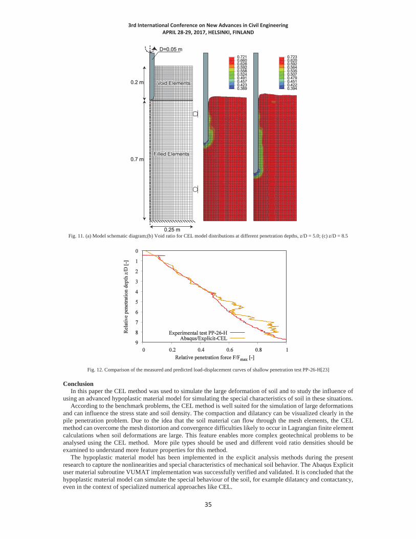
The schematic diagram of the problem shown in Fig. 11 shows a layer of void elements which allows the material to flow after the heaving of the soil occurs. The CEL method allows the flow of the material through the mesh elements without any distortion of the mesh. In Fig. 11 illustrates the void ratio distribution along the pile shaft which can be shown clearly the contraction along the pile shaft if formed as the typical experimental results. A good correlation between the results of the CEL model and the experiments carried out at TU-Berlin carried out at [23], see Fig. 12

Table 3. Hypoplastic parameters for the used soil model.

c [°] s [MPa] d0 c0 i0 por0 31.5 76.5 0.29 0.48 0.78 0.9 0.13 1 0.546 5.0 2.0 1x10-4 6.0 0.5


35

Fig. 11. (a) Model schematic diagram;(b) Void ratio for CEL model distributions at different penetration depths, z/D = 5.0; (c) z/D = 8.5

Fig. 12. Comparison of the measured and predicted load-displacement curves of shallow penetration test PP-26-H[23]

Conclusion

In this paper the CEL method was used to simulate the large deformation of soil and to study the influence of using an advanced hypoplastic material model for simulating the special characteristics of soil in these situations.

According to the benchmark problems, the CEL method is well suited for the simulation of large deformations and can influence the stress state and soil density. The compaction and dilatancy can be visualized clearly in the pile penetration problem. Due to the idea that the soil material can flow through the mesh elements, the CEL method can overcome the mesh distortion and convergence difficulties likely to occur in Lagrangian finite element calculations when soil deformations are large. This feature enables more complex geotechnical problems to be analysed using the CEL method. More pile types should be used and different void ratio densities should be examined to understand more feature properties for this method.

The hypoplastic material model has been implemented in the explicit analysis methods during the present research to capture the nonlinearities and special characteristics of mechanical soil behavior. The Abaqus Explicit user material subroutine VUMAT implementation was successfully verified and validated. It is concluded that the hypoplastic material model can simulate the special behaviour of the soil, for example dilatancy and contactancy, even in the context of specialized numerical approaches like CEL.


36

Acknowledgement

The present work has been done in the framework of the PhD thesis preparation for the corresponding author, which has a scholarship from the German Academic Exchange Service (DAAD). Furthermore, the authors appreciate the academic use of the commercial program Abaqus.

References [1] Benson D. Computational methods in Lagrangian and Eulerian hydrocodes. Computer Methods in Applied Mechanics and Engineering,

1992;99:235–394. [2] Aubram D., Rackwitz F., Savidis S. Contribution to the Non-Lagrangian Formulation of Geotechnical and Geomechanical Processes.

In: Triantafyllidis T (ed). Holistic Simulation of Geotechnical Installation Processes: Theoretical Results and Applications. Springer International Publishing, 2017:53–100

[3] Qiu G., Grabe J. Numerical investigation of bearing capacity due to spudcan penetration in sand overlying clay. Can. Geotech. J., 2012;49:1393–1407.

[4] Qiu G., Henke S., Grabe J. Application of a Coupled Eulerian–Lagrangian approach on geomechanical problems involving large deformations. Computers and Geotechnics, 2011;38:30–39.

[5] Wang D., Bienen B., Nazem M., Tian Y., Zheng J., Pucker T., Randolph M. Large deformation finite element analyses in geotechnical engineering. Computers and Geotechnics, 2015;65:104–114.

[6] Aubram D., Rackwitz F., Wriggers P., Savidis S. An ALE method for penetration into sand utilizing optimization-based mesh motion. Computers and Geotechnics, 2015;65:241–249.

[7] Aubram D. Über die Berücksichtigung großer Bodendeformationen in numerischen Modellen. Vorträge zum Ohde-Kolloquium, Dresden, Germany, 2014:109–122.

[8] Konkol J. Numerical solutions for large deformation problems in geotechnical engineering. PhD Interdisciplinary Journal, 2014:49–55.

[9] Qiu G., Henke S., Grabe J. Applications of Coupled Eulerian-Lagrangian Method to Geotechnical Problems with Large Deformations. SIMULIA Customer Conference, 2009.

[10] Taylor L., Cao J., Karafillis A., Boyce M. Numerical simulations of sheet-metal forming. Journal of Materials Processing Technology, 1995;50:168–179.

[11] Kutt L., Pifko A., Nardiello J., Papazian J. Slow-dynamic finite element simulation of manufacturing processes. Computers & Structures, 1998;66:1–17.

[12] Doweidar M., Calvo B., Alfaro I., Groenenboom P., Doblaré M. A comparison of implicit and explicit natural element methods in large strains problems: Application to soft biological tissues modeling. Computer Methods in Applied Mechanics and Engineering, 2010;199:1691–1700.

[13] Harewood F., McHugh P. Comparison of the implicit and explicit finite element methods using crystal plasticity. Computational Materials Science, 2007;39:481–494.

[14] Hilber H., Hughes T., Taylor R. Collocation, Dissipation and `Overshoot' for Time Integration Schemes in Structural Dynamics. Earthquake Engineering and Structural Dynamics, 1978;6:99–117.

[15] Sun J., Lee K., Lee H. Comparison of implicit and explicit finite element methods for dynamic problems. Journal of Materials Processing Technology, 2000;105:110–118.

[16] Dassault Systèmes, 2012. ABAQUS: Version 6.12 documentation. [17] von Wolffersdorff P-A. A hypoplastic relation for granular materials with a predefined limit state surface. Mech. cohesive-frictional

mater, 1996;1:251–271. [18] A. Niemunis, I. Herle. Hypoplastic model for cohesionless soils with elastic strain range. Mechanics of Cohesive-Frictional Materials,

1997;2:279–299. [19] Qiu G., Grabe J. Explicit modeling of cone and strip footing penetration under drained and undrained conditions using a visco-

hypoplastic model. geotechnik, 2011;34:205–217. [20] K. Nübel, Danzig, A. Niemunis. Finite element implementation of hypoplasticity - UMAT for von Wolffersdorff hypoplastic model.,

1998. [21] Reyes D., Rodriguez-Marek A., Lizcano A. A hypoplastic model for site response analysis. Soil Dynamics and Earthquake Engineering,

2009;29:173–184. [22] Hill R., 1998. The mathematical theory of plasticity. Oxford classic texts in the physical sciences;11. Clarendon Press, Oxford. [23] Aubram D., 2013. Arbitrary Lagrangian-Eulerian method for penetration into sand at finite deformations. Shaker Verlag, Aachen,

Germany. [24] Arslan H., Sture S. Finite element simulation of localization in granular materials by micropolar continuum approach. Computers and

Geotechnics, 2008;35:548–562.

GEOTECHNICAL LARGE DEFORM ATION NUMERICAL ANALYSIS … · GEOTECHNICAL LARGE DEFORM ATION NUMERICAL ANALYSIS USING IMPLICIT AND EXPLICIT INTEGRATION Montaser BAKROON1, Daniel AUBRAM2,Frank

Documents